1801.01554

## An Implementation of Back-Propagation Learning on GF11, a Large SIMD Parallel Computer Michael Witbrock and Marco Zagha December 1989 CMU-CS-89-208 School of Computer Science Carnegie Mellon University Pittsburgh, PA 15213 ## Abstract Current connectionist simulations require huge computational resources. We describe a neural network simulator for the IBM GF11, an experimental SIMD machine with 566 processors and a peak arithmetic performance of 11 Gigaflops. We present our parallel implementation of the backpropagation learning algorithm, techniques for increasing efficiency, performance measurements on the NetTalk text-to-speech benchmark, and a performance model for the simulator. Our simulator currently runs the back-propagation learning algorithm at 900 million connections per second, where each 'connection per second' includes both a forward and backward pass. This figure was obtained on the machine when only 356 processors were working; with all 566 processors operational, our simulation will run at over one billion connections per second. We conclude that the GF11 is well-suited to neural network simulation, and we analyze our use of the machine to determine which features are the most important for high performance. This research was performed at and supported by the IBM T.J. Watson Research Center, Yorktown Heights, NY 10598. The production of this Report was supported in part by Hughes Aircraft Corporation and National Science Foundation grant ECS-8716324. The views and conclusions contained in this document are those of the authors and should not be interpreted as representing the official policies, either expressed or implied, of the International Business Machines Corporation, the Hughes Aircraft Corporation, the National Science Foundation, or the U.S. Government. ## 1. Introduction The recent development of several new and effective learning algorithms has inspired interest in applying neural networks to practical problems such as road following by autonomous vehicles[14], speech recognition[9], story understanding[12] and sonar target identification[7]. Many of these applications have been approached using variants of the Backpropagation learning algorithm[16]. Although this learning algorithm has been used to attack small problems with considerable success, the huge computational resources required have hindered attempts on large scale tasks. One of the authors of this paper has recently been involved in an attempt, at Carnegie Mellon University, to apply backpropagation learning to the problem of speaker-independent continuous speech recognition [6]. Even for the relatively small digit recognition task initially selected[11], it has been necessary to train rather large recurrent nets[4] by making around 10,000 passes through very large amounts of data. 1 On the Convex C-1 used for these experiments, a typical training run took about a week. It became clear that the connectionist simulation tools available to us would make it very difficult to approach the ultimate goal of learning to transcribe continuously spoken general English. A simulator several orders of magnitude faster might permit a worthy attack. The construction of such a simulator became feasible when the authors were offered the opportunity to write connectionist software for IBM's GF11 parallel supercomputer. ## 2. 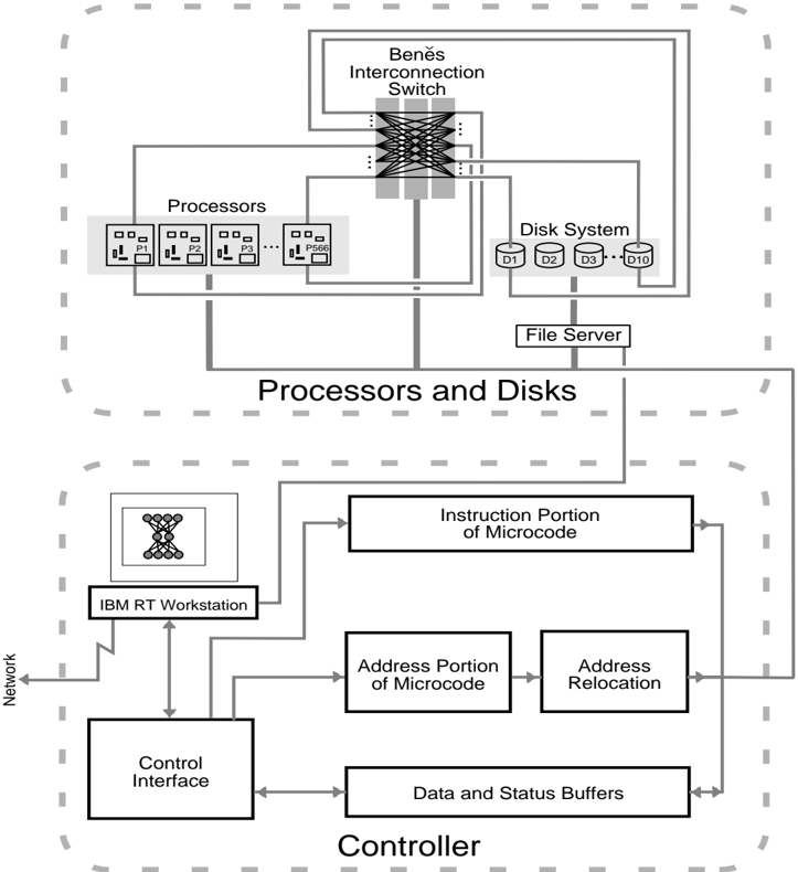GF11 Architecture and Microcode Generation GF11 [1] is an experimental parallel computer located at IBM's T.J. Watson Research Center at Yorktown Heights, New York. It is a SIMD (Single Instruction Multiple Data) machine composed of 566 processors interconnected through a Benˇ es Network[2] (See Figure 1). Each processor is capable of 20 million floating or fixed point operations per second, a rate which can be sustained during many kinds of calculations since intermediate results can be stored in a relatively large (256 word) register file. The registers can do up to four operations on every clock: write each of two operands to an ALU, read a result from an ALU, and write to or read from the interconnection network or static RAM (SRAM). Each processor has 16K words of static RAM, which, since it can be written or read on every clock, is effectively 4 times slower than the register file, and 512K words of dynamic RAM (DRAM), which is 4 times slower still. The Benˇ es network is capable of connecting the processors in arbitrary 1 to 1 permutations; 1024 such permutation patterns can be set up in the machine at once 2 . The whole machine has a peak arithmetic performance of 11.4 Gigaflops and contains a total of 1.14 Gbytes of semi-conductor memory. Programs for GF11 consist of subroutines of sequential (non-branching) microcode residing on 1 This long training period was necessary, even using the quickprop[5] variation of backprop which usually converges considerably faster than ordinary backprop. 2 Avariety of other connection topologies, including broadcasts and multicasts are also possible, but were relatively difficult to set up with the available software and were not needed for our purposes. Figure 1: The Architecture of the GF11 Computer (after Beetem[1]). <details> <summary>Image 1 Details</summary>  ### Visual Description ## System Diagram: Multiprocessor System Architecture ### Overview The image is a system diagram illustrating the architecture of a multiprocessor system. It shows the interconnection of processors, a disk system, and a controller, highlighting data flow and control mechanisms. ### Components/Axes * **Processors:** A group of processors labeled P1, P2, P3, and P566. * **Beněs Interconnection Switch:** A switch that connects the processors to the disk system. * **Disk System:** A set of disks labeled D1, D2, D3, and D10. * **File Server:** A component connecting the processors and disks. * **IBM RT Workstation:** A workstation connected to the controller. * **Control Interface:** An interface for controlling the system. * **Instruction Portion of Microcode:** A component related to microcode instructions. * **Address Portion of Microcode:** A component related to microcode addresses. * **Address Relocation:** A component for address relocation. * **Data and Status Buffers:** Buffers for data and status information. * **Network:** A connection to a network. * **Processors and Disks:** A grouping of the processors, interconnection switch, disk system, and file server. * **Controller:** A grouping of the IBM RT Workstation, Control Interface, Instruction Portion of Microcode, Address Portion of Microcode, Address Relocation, and Data and Status Buffers. ### Detailed Analysis * **Processors:** Four processors are explicitly labeled: P1, P2, P3, and P566. The processors are connected to the Beněs Interconnection Switch. * **Beněs Interconnection Switch:** This switch facilitates communication between the processors and the disk system. It is positioned at the top-center of the diagram. * **Disk System:** The disk system consists of four disks: D1, D2, D3, and D10. It is connected to the Beněs Interconnection Switch. * **File Server:** The file server acts as an intermediary between the processors and the disk system. * **IBM RT Workstation:** The workstation is connected to the Control Interface and the Instruction Portion of Microcode. * **Control Interface:** The control interface is connected to the IBM RT Workstation, the Data and Status Buffers, and the Address Portion of Microcode. * **Instruction Portion of Microcode:** This component is connected to the IBM RT Workstation and the Data and Status Buffers. * **Address Portion of Microcode:** This component is connected to the Control Interface and the Address Relocation component. * **Address Relocation:** This component is connected to the Address Portion of Microcode and the Data and Status Buffers. * **Data and Status Buffers:** This component is connected to the Control Interface, the Instruction Portion of Microcode, and the Address Relocation component. * **Network:** The network is connected to the IBM RT Workstation. ### Key Observations * The diagram shows a clear separation between the "Processors and Disks" section and the "Controller" section. * The Beněs Interconnection Switch is a key component for connecting processors and disks. * The IBM RT Workstation appears to be a central point for control and monitoring. * The flow of data and control signals is indicated by arrows. ### Interpretation The diagram illustrates a multiprocessor system architecture where multiple processors can access a shared disk system through an interconnection switch. The controller manages the operation of the system, with the IBM RT Workstation providing a user interface. The microcode components (Instruction Portion, Address Portion, and Address Relocation) likely handle low-level control and memory management. The data and status buffers facilitate communication between different components of the controller. The network connection allows for remote access and monitoring of the system. The architecture suggests a system designed for parallel processing and data-intensive applications. </details> a single, system wide controller. All of GF11's 566 processors receive exactly the same instruction at exactly the same time. Typically each processor will apply the instructions to different data, and, because the processors have a table lookup facility, this data can reside at different local memory addresses on different processors. The controller is connected to an IBM RT Workstation, which schedules the execution of microcode subroutines residing in the controller, and which can read results from and write data to GF11's processors via the controller. The controller is capable of storing 512K microcode instructions, a length which which corresponds to about 1/40th of a second of GF11 run-time. Only very limited data dependent computation is possible in this code: table lookup , and selection of the source (data path) from which an operand is taken. Since neither branching nor looping is possible in the microcode, program flow control must be implemented by having the RT choose which stored microcode subroutine to run next. Since memory addresses contained in the microcode may be mapped onto different physical addresses (relocated) by the controller, one can loop through large arrays by repeatedly applying a single section of sequential microcode to different portions of processor memory. Programming GF11 is straightforward. One can regard it as a vast floating point coprocessor attached to the RT. GF11 programs are programs written in a high level language 3 which run on the RT. At appropriate points in the program, functions are called to write data to, read data from, or execute a particular microcode subroutine on GF11. Microcode subroutines are, in turn, written as a series of calls to high-level language functions representing GF11 processor instructions such as floating add, write to memory, read from switch, etc. During a preliminary 'generation' execution of the program, these high level language subroutines are executed, and the GF11 operations required to perform their function are recorded. These operations are then passed through a scheduler and turned into a block of sequential microcode, which will execute on GF11 when the routine is called during a 'run' execution. Two advantages accrue from generating microcode by actually executing a high level program. The first advantage is that high level language constructs, such as loops and branches can be interspersed with the GF11 instructions, allowing the same block of high level language to generate many different microcode subroutines, depending on the state of program variables during 'generation'. This flexibility allowed our program to handle arbitrary network topologies very simply. Efficient, sequential microcode is generated by the program according to a topology file that it reads during 'generation'. In effect, our program compiles arbitrary feed-forward networks into GF11 microcode. The second advantage is that simulation of GF11 operation is virtually free. The routines representing GF11 operations are capable, depending on a mode switch, of outputting a GF11 microcode instruction, or of simulating execution of that instruction. We made a great deal of use of this simulation facility when developing and debugging our program. ## 3. The Backpropagation Learning Algorithm Backpropagation is a technique for training networks of simple neuron-like units connected by adjustable weights to perform arbitrary input/output mappings. Patterns are presented by setting the activation of a set of 'input layer' units. Activation flo ws forward to units in subsequent layers via adjustable weights, eventually reaching the output layer. The activation of a unit is calculated by computing the weighted sum of the activations of the units connected to it and then applying a squashing, or logistic, function 4 to it. The object of learning is to minimize the value of some error metric 5 between the actual activations of the output units, and the values required by the desired input/output mapping. This is done by computing the effect of each weight on the error metric, and adjusting the weight in the direction of reduced error. Since both the weighted sum and the logistic function are differentiable, this can be done by computing partial derivatives of the error measure with respect to each weight, starting with the weights to the output units and working backwards. 3 in the case of this simulator, the language used was a proprietary IBM language similar to PL1. 4 Usually the sigmoid function, 1 1+ e x . 5 Usually summed squared difference. /0 While in the 'online' version of backprop, the required weig ht changes are applied as they are computed, in our implementation, the changes required to reduce the error measure for each input/output pattern are accumulated across all patterns and used to compute a net (or 'pooled') weight update after all cases have been presented. Pooled update differs from the online version of the backpropagation algorithm in the following way: if there are np input-output pairs in the training sequence, online update allows np weight changes to be applied, whereas the most extreme form of pooled update allows only 1. For some data-sets (the NetTalk training set among them), this is a decided disadvantage. Using online update, NetTalk can be learned in 10 complete passes through the training set[3], a performance unlikely to be matched by the 10 updates allowed by strict pooled update. It is, however, an open question whether pooled update is worse in general. For some tasks, it appears to work better; in some recent experiments performed by one of the authors (Witbrock) - training recurrent networks for speech recognition - online backprop, even wit h a very small learning rate, had a tendency to reach a plateau beyond which it could not successfully reduce the error. With pooled update, this effect was not noticed. Pooled update also allows one to store successive approximations to the slope of the weight space with respect to the training set, permitting the use of the Quickprop weight update rule. This rule converges considerably more quickly that the usual update rule for many problems [5, 10]. Finally, the apparent disadvantage of pooled update is reduced when observes that update doesn't have to be pooled over all np patterns. In fact, weights can be updated after one case has been processed on each processor. ## 4. Simulator Implementation ## 4.1. Parallelizing Backprop for GF11 There are two obvious approaches to parallelizing backprop. In one approach, one divides the network, distributing 'neural processing units' - weig hts, units, or layers of units - across physical processors, and communicates activation levels between processors. In the other approach one can parallelize across training cases, having each processor simulate identical networks, but apply them to different subsets of training examples, communicating collected weight changes at the end of each training epoch (i.e. after a single presentation of each training example). Both approaches have been used in previous simulators. Blelloch and Rosenberg, in their simulator for the Connection Machine, mapped both individual weights and units to processors. The simulator on Warp initially mapped subsets of units with their corresponding weights to physical processors, but was later changed to the more efficient (on the Warp) case-based parallelism. Kevin Lang's [personal communication] simulator for the Convex C-1 Vector processor, and its descendants 6 all succeed in making backprop vectorizable by parallelizing across training cases. Dividing units across processors is a technique which appears to be best suited to MIMD machines with very fast communications - MIMD, because diff erent units in a neural network 6 Written by Franzini and Witbrock. 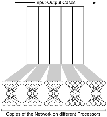Figure 2: Parallelizing backprop for GF11 <details> <summary>Image 2 Details</summary>  ### Visual Description ## Diagram: Parallel Processing of Input-Output Cases ### Overview The image illustrates a parallel processing architecture where multiple copies of a neural network are deployed on different processors to handle multiple input-output cases simultaneously. The diagram shows the flow of data from input-output cases to the network copies. ### Components/Axes * **Title:** The diagram does not have an explicit title, but the elements suggest it represents parallel processing. * **Top:** "Input-Output Cases" - Represents the input data being processed. This is depicted as a large rectangle divided into five equal vertical sections. * **Bottom:** "Copies of the Network on different Processors" - Represents the multiple instances of the neural network. * **Connections:** Gray shaded areas connect each section of the "Input-Output Cases" to a corresponding network copy. * **Network Structure:** Each network copy consists of three layers of nodes. The first layer has 4 nodes, the second layer has 2 nodes, and the third layer has 4 nodes. All nodes are fully connected to the nodes in the adjacent layers. ### Detailed Analysis * **Input-Output Cases:** The rectangle at the top is divided into five equal sections, implying five distinct input-output cases being processed in parallel. * **Network Copies:** There are five identical neural network structures at the bottom, each representing a copy of the network running on a different processor. * **Data Flow:** The gray shaded areas indicate the flow of data from each input-output case to its corresponding network copy. The shading suggests a distribution or mapping of the input data to the network. * **Network Architecture:** Each network has a simple feedforward architecture. The connections between the layers are fully connected. ### Key Observations * The diagram emphasizes the parallel nature of the processing, with each input-output case being handled by a separate network copy. * The network architecture is relatively simple, consisting of only three layers. * The diagram does not provide specific details about the type of neural network or the nature of the input-output cases. ### Interpretation The diagram illustrates a basic parallel processing approach for handling multiple input-output cases using neural networks. By deploying multiple copies of the network on different processors, the system can process multiple inputs simultaneously, potentially improving performance and throughput. The diagram highlights the concept of data parallelism, where the input data is divided and processed concurrently. The use of a simple network architecture suggests that this approach could be applied to a variety of tasks where parallel processing is beneficial. The diagram does not provide information about the specific application or the performance characteristics of the system. </details> have different patterns of connection, and very fast communication because activation levels must be passed between processors for each pattern presentation. If both units and weights are divided across processors, SIMD suffices, since all weights (and all units) are essentially the same, but even more communication is necessary 7 . For SIMD machines with moderate numbers of processors and sufficient memory on each processor, the technique of having each processor run the same network (and hence the same code) over a different subset of cases maps more neatly onto the architecture. This latter technique is the one that we used when designing our simulator. The ability to parallelize backprop across cases assumes that the changes to weights due to each input/output pattern are independent. That is, we must be able to satisfy the condition that the weight changes from the each of patterns in the training set can be applied in any order and yield the same result. This condition is clearly not satisfied by the canonical version of backprop, in which weight changes are calculated and applied after each pattern presentation. Instead, we use the 'pooled update' technique where weight changes are summ ed across all input/output cases, and the net change is applied after the entire training set 8 has been presented. When the algorithm is parallelized this way on GF11, each processor stores the input/output cases it is responsible for (See figure 2). It also has its own copy of the entire network (both units and weights), and storage for accumulating the total weight change due to its cases. After all the processors have finished calculating weight changes for all their cases, they share their accumulated weight changes with the other processors over the interconnection switch. They then update their local weights with the resulting total weight change over all cases. 7 In fact, Blelloch and Rosenberg report that communication speed was the primary limitation on the speed of their Connection Machine simulator. 8 Or a large enough subset of it to parallelize over. ## 4.2. Simulator Structure Dividing the functionality of the simulator into blocks of microcode is straightforward, although there are a few software and hardware imposed constraints. The current software restricts the size of microcode blocks to 20K lines. The hardware design forces the programmer to work within the memory limits of the machine - in particular, the 256 word register file and the total size of microcode memory (512K lines). We process weights by subsets of layers, or bundles , typically on the order of 1000 weights. This enables us to keep all the inputs and outputs of units in registers. To save microcode, we use the same microcode for all training examples and simply set a pointer to the current example in the controller. Similarly, when updating weights, we repeatedly set pointers to the weights and weight changes and call a routine to update a small group of weights. ## 4.3. Processor Dependent Computation Even when parallelization over cases is used to fit the algorithm to its SIMD architecture, there is still a problem with implementing backprop on the GF11. The problem arises because of the necessity of computing the sigmoid function 1 1+ e /0 x , on processors which can not perform division, let alone exponentiation, of floating point numbers. They can, however, do addition, multiplication, and a few other IEEE floating point operations including, perhaps most importantly, extracting the integer part of a floating point number ( /98 x /99 ). They can also do table lookup within SRAM, and can select the source of operands depending on condition codes set as a result of previous operations (the 'select' operation). Two methods of computing the sigmoid function were tried, using both forms of processor dependent computation available. 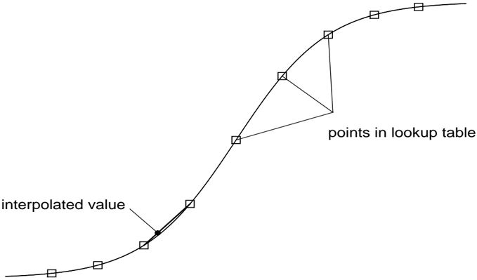The second approach to computing the sigmoid function involved using the 'select' operation (data dependent data path selection) to ensure that values of x were in the range [ /0 15; 15]. Values outside of this range were mapped to the extreme values of the sigmoid function. Numbers within the range were remapped, by addition and multiplication, as x 1 over a range of [0; 255]. The integer part /98 x 1 /99 of these numbers was used to do table lookup into a precomputed table of 1 1+ e /0 x ; the fractional part of the number, x 1 /0 /98 x 1 /99 , was used to perform linear interpolation between successive entries in the lookup table. Using this combination of table lookup and interpolation, 9 any differentiable monotonic function over the reals is usable The first approach involved replacing the sigmoid function with 1 1+2 /0 x , or equivalently, 9 2 x 2 x +1 . To help compute 2 x , we use the identity 2 x = 2 x 2 2 and a polynomial approximation for 2 x accurate in the range [0 /58 0; 0 /58 5]. More precisely, we compute 2 /98 x /99 2 x /0/98 x /99 2 2 , where 2 /98 x /99 is computed by table lookup. This reformulation reduces the required operations to addition, multiplication and round down, all of which are provided by the hardware, and taking the reciprocal of a number, which was available as an accurate library routine. Figure 3: Computing sigmoid by table lookup. Actual table contained 256 points. <details> <summary>Image 3 Details</summary>  ### Visual Description ## Curve Diagram: Interpolation Illustration ### Overview The image is a diagram illustrating the concept of interpolation using a lookup table. A smooth curve is shown, with discrete data points (represented by squares) sampled along the curve. An interpolated value is highlighted, demonstrating how a value between the sampled points can be estimated. ### Components/Axes * **Curve:** A smooth, black line representing a continuous function. * **Data Points:** Represented by small, open squares along the curve. These are labeled as "points in lookup table". * **Interpolated Value:** A solid black dot on the curve, indicating a value estimated between the data points. * **Labels:** * "points in lookup table": Indicates the discrete data points. * "interpolated value": Indicates the estimated value on the curve. ### Detailed Analysis * **Curve Trend:** The curve starts with a shallow slope, gradually increases in steepness, and then flattens out again. It resembles an S-shaped curve. * **Data Points:** The open squares are positioned along the curve, representing discrete samples. The spacing between the squares appears relatively uniform. * **Interpolated Value:** The black dot is located on the curve between two data points. A line connects the dot to the curve, and an arrow points to the dot from the label "interpolated value". * **Lookup Table Points Connection:** A triangle connects three of the lookup table points. ### Key Observations * The diagram clearly illustrates how interpolation is used to estimate values between known data points. * The curve represents the underlying continuous function, while the data points represent the discrete samples stored in a lookup table. * The interpolated value is an approximation of the true value on the curve, based on the surrounding data points. ### Interpretation The diagram demonstrates the concept of interpolation, a technique used to estimate values between known data points. In this case, the curve represents a continuous function, and the squares represent discrete samples stored in a lookup table. The interpolated value is an approximation of the true value on the curve, based on the surrounding data points. This is a common technique used in computer graphics, signal processing, and other fields where continuous functions are approximated using discrete data. The triangle connecting three of the lookup table points is likely meant to illustrate how interpolation can be performed using multiple points. </details> the sigmoid function could be computed with approximately five decimal places of accuracy over its entire domain. See figure 3. There were two other, less important, pieces of code where the 'select' operation was used. One use was to replace outlandish weight changes by zero, so that the hardware errors which were frequent while we were developing our code would not render the algorithm unworkable (see section 8 below). The other use of data dependent data path selection was in an (unfinished) implementation of Fahlman's quickprop weight update rule[5], which includes a number of calculation steps which are dependent on the local curvature of the error surface in weight space. ## 4.4. Processor Communication ## 4.4.1. 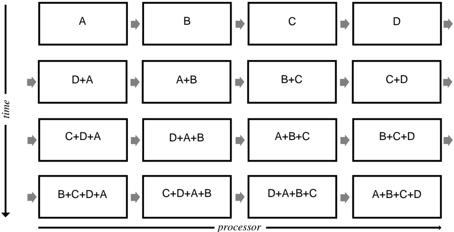Summing Weight Changes in a Ring In our initial approach, we used one switch configuration to connect P processors in a ring and sum each weight change in P steps. On the first step, each processor initializes Sum to zero and loads its weight change into the variable Neighbor . Then for remaining P /0 1 steps, each processor sends Neighbor to the processor on its right, receives a new value of Neighbor from the processor on its left, and adds Neighbor to Sum . At the end of P steps each processor has the same value for the total weight change in Sum (See figure 4). This algorithm has a time complexity of O ( NPROCS ) per weight. Figure 4: Summing Weight Changes with Processors Configured in a Ring <details> <summary>Image 4 Details</summary>  ### Visual Description ## Diagram: Processor Task Flow ### Overview The image is a diagram illustrating the flow of tasks across processors over time. It depicts a sequence of operations, where individual tasks (A, B, C, D) are combined and processed sequentially. The diagram is organized in a grid format, with the horizontal axis representing the processor and the vertical axis representing time. Each cell in the grid represents a processing stage, showing the combination of tasks being processed at that stage. ### Components/Axes * **Horizontal Axis:** Labeled "processor," indicating the progression of tasks across different processing units. * **Vertical Axis:** Labeled "time," indicating the temporal sequence of the tasks. The arrow points downwards, indicating the direction of time. * **Rectangular Boxes:** Each box represents a processing stage, containing the tasks being processed at that stage. * **Arrows:** Gray arrows indicate the flow of tasks from one processing stage to the next. ### Detailed Analysis The diagram consists of a 4x4 grid of rectangular boxes, each containing a combination of tasks (A, B, C, D). The tasks are processed sequentially, with the output of one stage becoming the input of the next. **Row 1 (Top Row):** * Box 1: A * Box 2: B * Box 3: C * Box 4: D **Row 2:** * Box 1: D+A * Box 2: A+B * Box 3: B+C * Box 4: C+D **Row 3:** * Box 1: C+D+A * Box 2: D+A+B * Box 3: A+B+C * Box 4: B+C+D **Row 4 (Bottom Row):** * Box 1: B+C+D+A * Box 2: C+D+A+B * Box 3: D+A+B+C * Box 4: A+B+C+D The arrows indicate the flow of tasks from left to right (across processors) and from top to bottom (over time). ### Key Observations * The tasks are combined sequentially, with each stage adding a new task to the combination. * The order of tasks in each combination appears to be consistent within each row. * The diagram illustrates a pipeline processing model, where tasks are processed in parallel across multiple processors. ### Interpretation The diagram illustrates a pipeline processing model where tasks A, B, C, and D are processed sequentially across multiple processors. The "processor" axis represents the progression of tasks through different processing units, while the "time" axis represents the temporal sequence of the tasks. Each box represents a processing stage, where the tasks are combined and processed. The diagram demonstrates how tasks can be processed in parallel to improve overall throughput. The sequential combination of tasks suggests a dependency relationship, where each task relies on the output of the previous stage. The diagram could represent a simplified model of a complex processing system, such as a compiler or a data processing pipeline. </details> ## 4.4.2. Summing Weight Changes in a Tree GF11's powerful communication facility allows a more efficient approach to summing weight changes. We use several switch configurations to sum weight changes in a binary tree using a standard data-parallel algorithm[8]. 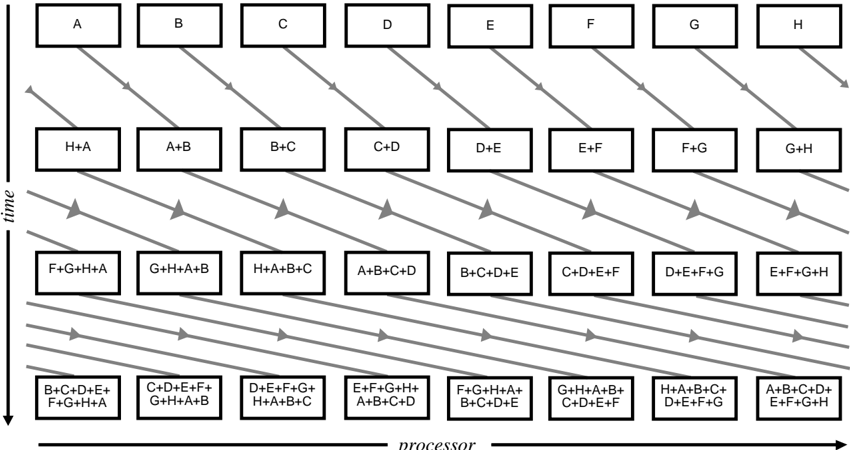On step i (starting at zero), processor P sends its weight change to processor ( P + 2 i ) mod NPROCS and adds the weight change it received to its weight change. After log 2 NPROCS steps, the total weight change in each processor contains the sum of the individual weight changes. See figure 5. This algorithm has a time complexity of O (log 2 NPROCS ) per weight. If the number of processors is not a power of 2, we generate two additional communication instructions. Call each processor /102 Pn : n /62 2 /98 log 2 NPROCS /99 /103 a 'leftover' processor. Each leftover processor Pn sends its weight change to its 'buddy', processor number n /0 2 /98 log 2 NPROCS /99 , which adds the value to its weight change. Then logarithmic summing proceeds as described above. Finally, each leftover processor receives the final total weight change from its buddy. During the two extra steps, processors not involved in the communication mask out their operations using condition codes. <details> <summary>Image 5 Details</summary>  ### Visual Description ## Diagram: Processor Task Dependency ### Overview The image is a diagram illustrating the dependencies of tasks across multiple processors over time. It shows how the output of one task (represented by a letter) is used as input for subsequent tasks, both on the same processor and across different processors. The diagram visualizes a parallel processing workflow, where tasks are chained together, and the completion of one task triggers the start of another. ### Components/Axes * **X-axis:** Labeled "processor," representing different processing units. * **Y-axis:** Labeled "time," indicating the progression of tasks. * **Nodes:** Rectangular boxes representing tasks, labeled with letters (A, B, C, D, E, F, G, H) or combinations of letters (e.g., H+A, A+B+C+D). * **Arrows:** Gray arrows indicating the flow of data and dependencies between tasks. The arrows point diagonally downwards from left to right. ### Detailed Analysis The diagram can be broken down into rows representing different time steps. * **Row 1 (Top):** * Tasks A, B, C, D, E, F, G, and H are initiated on separate processors. * **Row 2:** * Task H+A depends on the output of tasks H and A. * Task A+B depends on the output of tasks A and B. * Task B+C depends on the output of tasks B and C. * Task C+D depends on the output of tasks C and D. * Task D+E depends on the output of tasks D and E. * Task E+F depends on the output of tasks E and F. * Task F+G depends on the output of tasks F and G. * Task G+H depends on the output of tasks G and H. * **Row 3:** * Task F+G+H+A depends on the output of tasks F+G and H+A. * Task G+H+A+B depends on the output of tasks G+H and A+B. * Task H+A+B+C depends on the output of tasks H+A and B+C. * Task A+B+C+D depends on the output of tasks A+B and C+D. * Task B+C+D+E depends on the output of tasks B+C and D+E. * Task C+D+E+F depends on the output of tasks C+D and E+F. * Task D+E+F+G depends on the output of tasks D+E and F+G. * Task E+F+G+H depends on the output of tasks E+F and G+H. * **Row 4 (Bottom):** * Task B+C+D+E+F+G+H+A depends on the output of tasks F+G+H+A. * Task C+D+E+F+G+H+A+B depends on the output of tasks G+H+A+B. * Task D+E+F+G+H+A+B+C depends on the output of tasks H+A+B+C. * Task E+F+G+H+A+B+C+D depends on the output of tasks A+B+C+D. * Task F+G+H+A+B+C+D+E depends on the output of tasks B+C+D+E. * Task G+H+A+B+C+D+E+F depends on the output of tasks C+D+E+F. * Task H+A+B+C+D+E+F+G depends on the output of tasks D+E+F+G. * Task A+B+C+D+E+F+G+H depends on the output of tasks E+F+G+H. ### Key Observations * Each task in a row depends on the output of two tasks from the previous row. * The dependencies shift diagonally, indicating that data is being passed between processors. * The complexity of the tasks increases over time, as more data is combined. ### Interpretation The diagram illustrates a parallel processing pipeline where data is processed in stages. Each processor performs a specific task, and the output of that task is passed to the next processor in the pipeline. This allows for efficient processing of large amounts of data, as multiple processors can work on different parts of the data simultaneously. The diagram demonstrates how tasks are chained together and how data flows between processors to achieve a final result. The increasing complexity of tasks over time suggests that the pipeline is designed to perform increasingly complex operations on the data as it progresses through the system. </details> processor Figure 5: Summing Weight Changes with Processors Configured in a Tree ## 5. Simulating Larger Networks As described so far, our implementation could only accommodate networks with a few thousand weights within the 16K word SRAM. Training examples can be kept in DRAM with trivial changes to the code and a negligible performance penalty. However, without further changes to the structure or the program, keeping weights in DRAM creates a fundamental efficiency problem: transfers to and from DRAM would take over twice as long as the floating point computation. A transfer to or from DRAM can be started at most once per 4 cycles. However, in the forward pass only two floating point operations per weight are required, yielding a maximum efficiency of 50%. In the backward pass, a weight change and a weight must be loaded, add and weight change must be stored, requiring 3 transfers per 4 floating point operations, yielding only 33% efficiency. We adopt the following approach to obtain locality of reference to the weights and weight changes. Instead of doing independent forward and backward passes for each case, we move a bundle of weights and weight changes into an SRAM cache, process several training examples on those weights, and then move the weights values back to DRAM. The original structure of the simulator was the following: For each training example For each Sweep forward on bundle For each Sweep ``` for each bundle of weights Sweep forward on bundle for each bundle of weights (in reverse order) Sweep backward on bundle ``` ## The new structure that uses DRAM: ``` For each group of training examples For each bundle of weights Move weights to a cache in SRAM For each training example in group Sweep forward on bundle For each bundle of weights (in reverse order) Move weights and weight changes to a cache in SRAM For each training example in group Sweep backward on bundle Move weight changes from cache to DRAM ``` <details> <summary>Image 6 Details</summary>  ### Visual Description ## 3D Cube Diagram: Source, Destination, Case with SRAM Capacity ### Overview The image is a 3D cube diagram illustrating the relationship between "Source Unit", "Destination Unit", and "Case". A smaller cube labeled "SRAM Capacity" is positioned near the "Case" axis. The diagram appears to represent a conceptual model, possibly related to data processing or memory allocation. ### Components/Axes * **Axes:** * X-axis: "Destination Unit" * Y-axis: "Source Unit" * Z-axis: "Case" * **Labels:** * "one case" - Located near the Z-axis ("Case") * "SRAM Capacity" - Label for the smaller cube. * **Cube Representation:** * The larger cube represents the overall space defined by the three axes. * A shaded region is present on the top and right faces of the larger cube. * The smaller cube represents "SRAM Capacity". ### Detailed Analysis or Content Details * **Axes Labels:** The axes are labeled "Source Unit", "Destination Unit", and "Case". * **Large Cube:** The large cube has a shaded area on its top and right faces, indicating a specific region or condition within the overall space. * **Small Cube:** The small cube, labeled "SRAM Capacity", is located near the "Case" axis, suggesting a relationship between the case and SRAM capacity. * **"one case" Label:** The label "one case" is positioned close to the "Case" axis, possibly indicating a specific instance or scenario. ### Key Observations * The diagram uses a 3D cube to represent a relationship between three variables: Source Unit, Destination Unit, and Case. * The "SRAM Capacity" is represented as a separate, smaller cube, suggesting it's a factor related to the "Case". * The shaded region on the large cube might represent a specific condition or constraint within the overall space. ### Interpretation The diagram likely represents a conceptual model for understanding the relationship between data sources, destinations, and different cases, with SRAM capacity being a relevant factor. The shaded region on the large cube could indicate a specific operational range or constraint. The diagram suggests that SRAM capacity is somehow related to the "Case" dimension, possibly indicating that different cases require different amounts of SRAM. The diagram does not provide specific numerical data, but rather a visual representation of the relationships between these components. </details> Destination Unit Figure 6: Processing all the Weights for a Single Case. <details> <summary>Image 7 Details</summary>  ### Visual Description ## 3D Diagram: Source, Destination, Case ### Overview The image is a 3D diagram representing relationships between "Source Unit", "Destination Unit", and "Case". It includes two shaded cubes, one representing "Two cases over a subset of weights" and the other representing "SRAM Capacity". The diagram appears to illustrate a conceptual space where these elements interact. ### Components/Axes * **Axes:** * Vertical axis: "Source Unit" * Horizontal axis (extending into the page): "Destination Unit" * Axis extending to the right: "Case" * **Objects:** * Large cube outlining the space defined by the axes. * Small shaded cube near the origin, labeled "Two cases over a subset of weights". * Small shaded cube on the "Case" axis, labeled "SRAM Capacity". ### Detailed Analysis * **"Two cases over a subset of weights" Cube:** * Position: Located near the origin of the 3D space, indicating a low value for Source Unit, Destination Unit, and Case. * Description: The cube is shaded gray and appears to be composed of two stacked cubes. * Label: "Two cases over a subset of weights" is indicated by a curly bracket pointing to the cube. * **"SRAM Capacity" Cube:** * Position: Located along the "Case" axis, indicating a higher value for Case and low values for Source Unit and Destination Unit. * Description: The cube is shaded gray. * Label: "SRAM Capacity" is written below the cube. ### Key Observations * The diagram uses spatial positioning to represent the relationship between the three dimensions. * The "Two cases over a subset of weights" cube is closer to the origin, suggesting it represents a smaller or more fundamental element in the system. * The "SRAM Capacity" cube is positioned along the "Case" axis, indicating its primary association with the "Case" dimension. ### Interpretation The diagram seems to be a conceptual representation of how "Source Unit", "Destination Unit", and "Case" interact, with specific examples of "Two cases over a subset of weights" and "SRAM Capacity" placed within this space. The positioning of the cubes suggests their relative importance or association with each dimension. The diagram could be used to illustrate the relationships between different components in a system or to visualize the impact of different parameters on a particular outcome. The "Two cases over a subset of weights" likely represents a specific scenario or configuration, while "SRAM Capacity" represents a resource or constraint within the system. 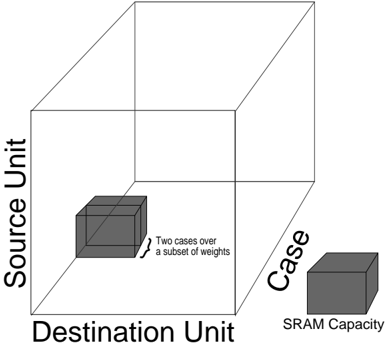</details> Figure 7: Processing a Subset of the Weights for Several Cases at Once. 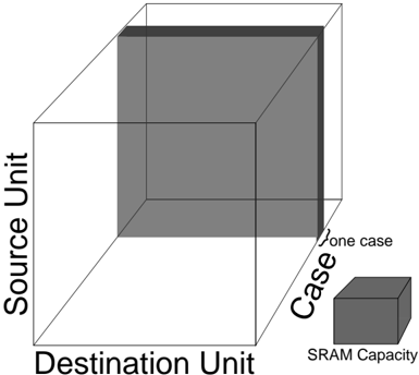As another way of understanding this change, the loop structure can be viewed as a traversal of points on a 3-dimensional rectangular grid. The points on the grid represent weights (or weight changes) and the axes of the grid are input unit index, output unit index, and training example index. In our original approach (see figure 6), we traverse one slice of the grid at once - that is we process one case at a time. We were forced to modify this algorithm because the memory required for this slice exceeds the capacity of free memory in SRAM. In the improved approach we traverse a sub-grid (See figure 7) which corresponds to several training examples processed on a subset of the weights. Since the weights are the same for each training example, we reduce transfers to and from DRAM. ## 6. Simulator Performance ## 6.1. Performance Model Developing a performance model yields several important benefits. Execution times for different topologies and training set sizes can be estimated without having to execute a program on GF11. The performance model can also approximate the optimal number of processors to use for a given problem. More importantly, the model makes analyzing the role of the simulator components much easier. Bottlenecks are revealed, and the importance of specific machine features can be determined. Several assumptions are implicit in the performance model. We neglect computation on units, such as the sigmoid calculation, since there are typically many more weights than units. We also assume that computation during the forward and backward passes fills the processor pipeline this amounts to assuming more than 12 units per layer. | Let | G = number of groups of training cases | |---------------------------------------------------------------------|------------------------------------------| | W = total number of weights W i = number weights in the input layer | U = number of units | | B = maximum number of weights in a bundle | M = number of free words in SRAM | | C = number of training cases | P = number of processors | In the forward pass, one add and one multiply per weight are executed: $$C y c l e s f o r w a r d / c a s e = 2 W$$ In the backward pass, two adds and two multiplies per weight are executed, except for connections from input units which execute one and and one multiply: ``` Cycles backward/case = 2 W _ { i } + 4 ( W - W _ { i } ) ``` /0 Transfers to or from DRAM can only be started once every 4 cycles. In the forward pass, each weight is transferred to SRAM once per group of training examples. In the backward pass, a weight change is loaded and stored once per group of examples, and weights not in the input layer are loaded once: Cycles forward weight transferring/group = 4 W Cycles backward transferring weight changes/group = (4)(2) W Cycles backward transferring weight/group = 4( W Wi ) $$C y c l e s \, p e r \, u p d a t e = 4 W \lceil \log _ { 2 } P \rceil$$ /0 Communications over the switch also can only be started once every 4 cycles. When summing in a tree: 10 /100 /101 When summing in a ring: Cycles per update = 4 WP After allocating space for the sigmoid lookup tables and a few other constants, the amount of free SRAM is approximately: $$M = 1 5 K$$ The weight value and weight change caches use 2 B words of memory, and two words per unit are used to hold unit activation and error levels. Thus, the size of a group of cases that can be processed entirely in SRAM is: The number of groups of cases is: /61 /2 /61 /0 Total time per epoch in cycles (when summing in a tree): T = 2 W C P + (2 Wi + 4( W Wi )) C P + (12 W + 4( W Wi )) G + 4 P W $$\frac { M - 2 B } { 2 U }$$ $$G = C / P \times ( 2 U / ( M - 2 B ) )$$ /2 /61 /0 /2 /61 /0 /2 /2 Because each processor executes 20 million instructions per second, millions of connections per second (MCPS) is simply, 20 T $$P = \frac { C } { 4 W } \times ( ( 6 W - 2 W _ { i } ) + \frac { 2 U } { M - 2 B } \times ( 1 6 W - 4 W _ { i } ) )$$ /61 To find the optimal number of processors when summing in a tree we differentiate time with respect to the number of processors, equate the result to zero, solve, and simplify: /2 /0 /0 /2 /0 When summing in a ring, the optimal number of processors is simply the square root of the above quantity. 10 if the number of processors is not a power of 2, there is one extra communication not counted in the model ## 6.2. Optimizing Microcode ## 6.2.1. Optimization Techniques Typically, the first attempt at implementing a microcode routine resulted in code running at less than 50% of optimal performance. In this section, we describe techniques for improving microcode efficiency. These techniques follow from two general principles of code optimization: breaking computation into carefully sized pieces to accomodate multi-level memory hierarchies, and reordering independent instructions to improve pipeline scheduling. Producing efficient microcode is difficult for a number of reasons. The processor pipeline is 25 deep - that is, the result of a floating point operation do es not appear for 25 cycles. In addition, several operations may execute in one cycle. Although pipeline scheduling is not the programmer's responsibility, the scheduling process is not completely invisible. The programmer often has to know what performance constraints the machine imposes and a few details of the scheduler implementation. The microcode scheduler rearranges instruction order but is constrained by the programmer's approach to data movement. Thus, managing the register/SRAM/DRAM hierarchy becomes the key to producing efficient microcode. In section 5 we discussed changes to the program structure to minimize DRAM traffic. To minimize SRAM traffic, we keep net inputs in registers during the forward pass rather than reloading the values to increment them. Similarly, during the backward pass, error into a unit is kept in registers. Using weight bundles instead of entire weight layers reduces the number of units used in a block of microcode and enables this strategy to work within the 256 register limit. Analyzing the output of the microcode scheduler is the next step after developing a reasonable approach to memory management. This phase can be tedious, but it often reveals problems that can fixed by changing the order of instructions or by inserting scheduler directives. For example, the routines that sum weight changes must loop over both communication steps and indices of weight changes. By simply interchanging the loops to sum all weight changes simultaneously, pipeline scheduling improves significantly. As another example, we improved the routine that sums weight changes in a ring by having it circulate weight increments rather than partial sums of weight increments. This change did not reduce the number of source instructions, but it did cut the number of dependent instructions in the critical path in half, since additions could be done in parallel with switch communication. Inefficient scheduling in the backward pass motivated one of the most interesting optimizations. In both the forward and backward passes, we ordered computation on weights by the unit on the input side of the weight. This turns out to work well for the forward pass, but not in the backward pass because for a M by N bundle of weights, the last M operations all increment the same register (the error from the last source unit). Since each operation must be separated by 25 cycles, this led to sub-optimal code. To improve efficiency, at microcode generation time, we simply create an ordering of weight indices for the backward pass sorted by output unit index. Then accesses to each of the M input units are separated by at least 2 N operations, which produces near optimal code for N greater than half the pipeline depth (i.e., N 12). /62 Interleaving code that is logically independent is the most difficult form of optimization, but is necessary for operations with a low throughput such as switch communication and transfers to and from DRAM. For example the routine responsible for updating weights performs several functions: it moves weights, weight changes, and weight changes from the previous epoch from DRAM to a cache in SRAM, sums weight deltas over the switch, calculates weight changes using the current value of the learning rate and momentum, updates the weights in the SRAM cache, moves the new weights back to DRAM, and zeroes weight changes in DRAM for the next epoch. Finally, because the DRAM is interleaved, accesses should be sequential whenever possible. ## 6.2.2. Microcode Efficiency In this section we report the efficiency of microcode routines generated for networks with at least 12 units per layer. We defer discussion of small networks until section 10.3. In the forward pass, 97-99% of all cycles execute an add or multiply. Memory transfers execute in parallel with floating point computation. In the backward pass, 85-99% of all cycles execute an add or multiply. This routine is slightly less efficient than the forward pass because of additional memory traffic - each weight requires both a load and store instead of just a load. Routines calculating the sigmoid and back error for units execute an add or multiply on about 40-70% of all cycles, which is fast enough to make the execution time negligible. Analyzing the performance for weight updating code is more complicated because we overlap DRAM transfers and computation with communication as described in the previous section. For simplicity, we adopt a pessimistic efficiency rating base on the number of switch communications only. Since each switch communication operation takes four cycles, we define the optimal number of cycles as four times the number of communications. When summing in a ring, we achieve 98% of optimal performance. DRAM transfers, weight update with momentum, and zeroing of weight changes for next epoch come for free in empty slots during communication. When summing in a tree, efficiency is approximately 60% of optimal performance because computation can not be fully overlapped with communication. Despite its lower execution efficiency , tree update takes considerably less time than ring update when more than 4 processors are used. ## 6.3. Performance Measurements We measured the performance on our simulator using NetTalk [17] text-to-phoneme benchmark (as did Pomerleau et al.[15] and Blelloch&Rosenberg [3]). The network consists of an input layer with 203 units and a 'true' unit, a hidden layer with 60 units, and an output layer of 26 units. 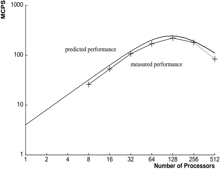The input layer is fully connected to the hidden layer, and the hidden layer is fully connected Figure 8: MCPS with Processors Configured in a Ring <details> <summary>Image 8 Details</summary>  ### Visual Description ## Chart: Predicted vs. Measured Performance ### Overview The image is a line chart comparing predicted and measured performance (in MCPS) against the number of processors. Both axes use a logarithmic scale. The chart shows how performance scales with an increasing number of processors, highlighting the difference between predicted and actual performance. ### Components/Axes * **Y-axis:** MCPS (Millions of Connections Per Second). Logarithmic scale with markers at 1, 10, 100, and 1000. * **X-axis:** Number of Processors. Logarithmic scale with markers at 1, 2, 4, 8, 16, 32, 64, 128, 256, and 512. * **Legend:** * "predicted performance": Represented by a solid black line. * "measured performance": Represented by '+' markers connected by a dotted black line after the 128 processor mark. ### Detailed Analysis * **Predicted Performance (Solid Black Line):** * Trend: Initially increases sharply, then plateaus and decreases slightly. * Data Points: * 1 processor: ~2 MCPS * 8 processors: ~25 MCPS * 32 processors: ~100 MCPS * 64 processors: ~150 MCPS * 128 processors: ~200 MCPS * 256 processors: ~180 MCPS * 512 processors: ~100 MCPS * **Measured Performance (+ Markers):** * Trend: Increases sharply, plateaus, and then decreases. * Data Points: * 8 processors: ~20 MCPS * 16 processors: ~40 MCPS * 32 processors: ~70 MCPS * 64 processors: ~120 MCPS * 128 processors: ~180 MCPS * 256 processors: ~160 MCPS * 512 processors: ~80 MCPS ### Key Observations * The predicted performance consistently overestimates the measured performance. * Both predicted and measured performance peak around 128 processors. * The measured performance starts to decline more sharply than predicted performance after 128 processors. ### Interpretation The chart illustrates the diminishing returns of adding more processors to a system. While the predicted performance suggests a continued increase (albeit at a slower rate) up to a certain point, the measured performance shows a clear peak and subsequent decline. This indicates that factors such as communication overhead or resource contention become significant bottlenecks as the number of processors increases. The divergence between predicted and measured performance highlights the importance of empirical testing and validation in system design. The logarithmic scales emphasize the exponential nature of the initial performance gains and the subsequent limitations. 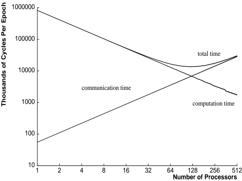</details> Figure 9: Communication and Computation with Processors Configured in a Ring <details> <summary>Image 9 Details</summary>  ### Visual Description ## Line Chart: Performance Scaling with Number of Processors ### Overview The image is a line chart illustrating the relationship between the number of processors used and the thousands of cycles per epoch for computation time, communication time, and total time. The x-axis represents the number of processors (ranging from 1 to 512), and the y-axis represents the thousands of cycles per epoch (ranging from 10 to 1,000,000) on a logarithmic scale. ### Components/Axes * **X-axis:** Number of Processors (scale: 1, 2, 4, 8, 16, 32, 64, 128, 256, 512) * **Y-axis:** Thousands of Cycles Per Epoch (logarithmic scale: 10, 100, 1000, 10000, 100000, 1000000) * **Data Series:** * **Computation Time:** A line that generally decreases as the number of processors increases. * **Communication Time:** A line that increases as the number of processors increases. * **Total Time:** A line that initially decreases, reaches a minimum, and then increases as the number of processors increases. ### Detailed Analysis * **Computation Time:** * At 1 processor, the computation time is approximately 1,000,000 cycles per epoch. * At 64 processors, the computation time is approximately 10,000 cycles per epoch. * At 512 processors, the computation time is approximately 1,000 cycles per epoch. * The line shows a decreasing trend, indicating that computation time decreases as the number of processors increases. The rate of decrease slows down as the number of processors increases. * **Communication Time:** * At 1 processor, the communication time is approximately 50 cycles per epoch. * At 64 processors, the communication time is approximately 5,000 cycles per epoch. * At 512 processors, the communication time is approximately 20,000 cycles per epoch. * The line shows an increasing trend, indicating that communication time increases as the number of processors increases. * **Total Time:** * At 1 processor, the total time is approximately 1,000,000 cycles per epoch. * The total time decreases until approximately 64 processors, where it reaches a minimum of approximately 10,000 cycles per epoch. * After 64 processors, the total time increases to approximately 20,000 cycles per epoch at 512 processors. * The line shows a U-shaped trend, indicating that total time initially decreases with more processors, but eventually increases due to communication overhead. ### Key Observations * Computation time decreases with an increasing number of processors, suggesting parallelization benefits. * Communication time increases with an increasing number of processors, indicating overhead associated with inter-processor communication. * Total time initially decreases, indicating that the benefits of parallelization outweigh the communication overhead. However, beyond a certain number of processors (around 64), the communication overhead becomes dominant, causing the total time to increase. ### Interpretation The chart demonstrates the trade-off between computation time and communication time when using multiple processors. Initially, adding more processors reduces the computation time significantly, leading to a decrease in total time. However, as the number of processors increases, the communication overhead becomes more significant, eventually outweighing the benefits of parallelization and causing the total time to increase. The optimal number of processors, in this case, appears to be around 64, where the total time is minimized. This suggests that there is a point of diminishing returns when adding more processors, and that careful consideration must be given to the communication overhead when designing parallel algorithms. 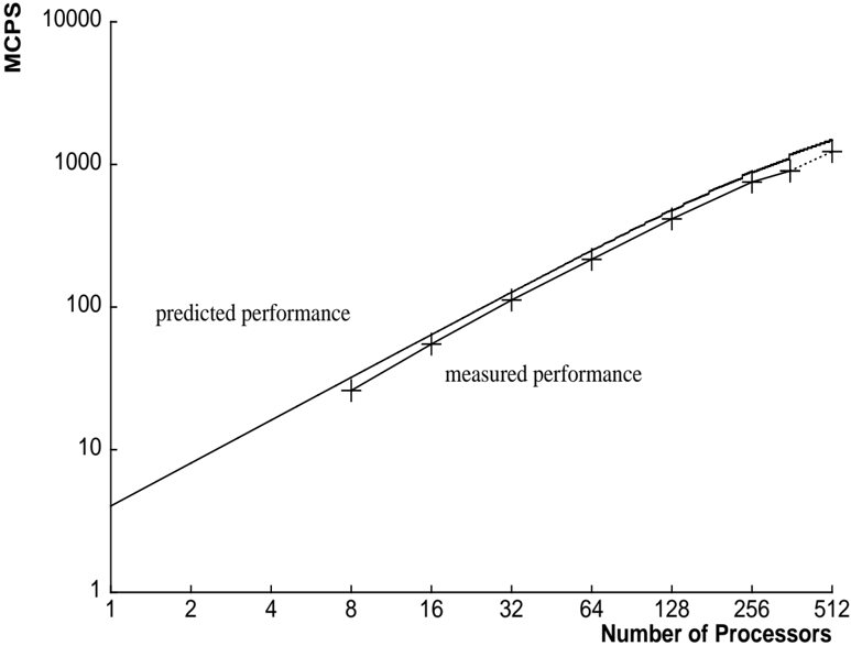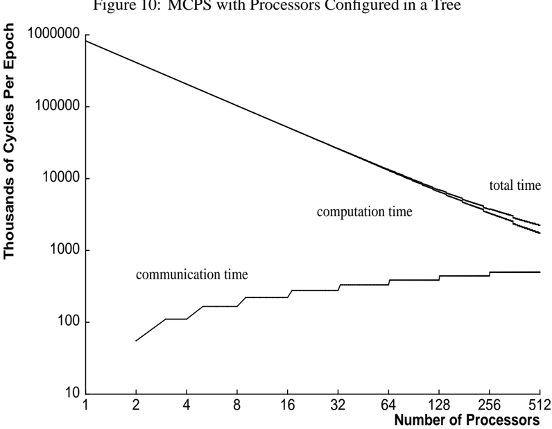</details> Figure 11: Communication and Computation with Processors Configured in a Tree <details> <summary>Image 10 Details</summary>  ### Visual Description ## Chart: Predicted vs. Measured Performance ### Overview The image is a line chart comparing predicted and measured performance, likely of a parallel computing system. The x-axis represents the number of processors, and the y-axis represents performance in MCPS (Millions of Connections Per Second). Both axes use a logarithmic scale. The chart displays two data series: "predicted performance" represented by a solid line, and "measured performance" represented by data points marked with "+" symbols connected by a solid line, which transitions to a dotted line at the higher end of the processor count. ### Components/Axes * **X-axis:** "Number of Processors" with a logarithmic scale. Axis markers are at 1, 2, 4, 8, 16, 32, 64, 128, 256, and 512. * **Y-axis:** "MCPS" (Millions of Connections Per Second) with a logarithmic scale. Axis markers are at 1, 10, 100, 1000, and 10000. * **Legend:** * "predicted performance" - represented by a solid line. Located in the center-left of the chart. * "measured performance" - represented by "+" markers connected by a solid line, transitioning to a dotted line. Located below "predicted performance". ### Detailed Analysis * **Predicted Performance:** The solid line representing predicted performance shows a consistent upward trend. * At 1 processor, the predicted performance is approximately 3 MCPS. * At 8 processors, the predicted performance is approximately 25 MCPS. * At 64 processors, the predicted performance is approximately 200 MCPS. * At 512 processors, the predicted performance is approximately 1600 MCPS. * **Measured Performance:** The data points connected by a line represent the measured performance. * At 1 processor, the measured performance is approximately 3 MCPS. * At 8 processors, the measured performance is approximately 20 MCPS. * At 64 processors, the measured performance is approximately 160 MCPS. * At 256 processors, the measured performance is approximately 800 MCPS. * At 512 processors, the measured performance is approximately 1100 MCPS, with the line becoming dotted, suggesting a potential change in behavior or prediction method. ### Key Observations * The predicted and measured performance are very close, especially at lower processor counts. * As the number of processors increases, the measured performance starts to deviate slightly from the predicted performance, with the measured performance being slightly lower than predicted. * The measured performance line transitions to a dotted line after 256 processors, suggesting a change in the model or a region where the prediction becomes less reliable. ### Interpretation The chart demonstrates the scaling of performance (MCPS) with an increasing number of processors. The close alignment of predicted and measured performance indicates a good model fit, especially at lower processor counts. The deviation at higher processor counts suggests that the model may need refinement or that other factors, such as communication overhead or resource contention, are becoming more significant and are not fully captured by the model. The dotted line for measured performance beyond 256 processors implies that the model's predictive power decreases or that the measurement method changes in this region. Overall, the chart provides insights into the scalability of the system and the accuracy of the performance model. </details> <details> <summary>Image 11 Details</summary>  ### Visual Description ## Chart: MCPS with Processors Configured in a Tree ### Overview The image is a line chart comparing the "total time", "computation time", and "communication time" in thousands of cycles per epoch against the number of processors, ranging from 1 to 512. The y-axis is logarithmic, spanning from 10 to 1,000,000. ### Components/Axes * **Title:** Figure 10: MCPS with Processors Configured in a Tree * **X-axis:** Number of Processors (1, 2, 4, 8, 16, 32, 64, 128, 256, 512) * **Y-axis:** Thousands of Cycles Per Epoch (10, 100, 1000, 10000, 100000, 1000000) * **Data Series:** * Total Time (Black): Decreases as the number of processors increases. * Computation Time (Black): Decreases as the number of processors increases, but at a slower rate than total time. * Communication Time (Black): Increases as the number of processors increases, but the rate of increase slows down as the number of processors increases. ### Detailed Analysis * **Total Time:** * At 1 processor: Approximately 800,000 cycles per epoch. * At 512 processors: Approximately 2,000 cycles per epoch. * Trend: Decreases sharply initially, then the rate of decrease slows down. * **Computation Time:** * At 1 processor: Approximately 80,000 cycles per epoch. * At 512 processors: Approximately 1,500 cycles per epoch. * Trend: Decreases as the number of processors increases. * **Communication Time:** * At 2 processors: Approximately 40 cycles per epoch. * At 512 processors: Approximately 400 cycles per epoch. * Trend: Increases in a step-wise fashion as the number of processors increases. The rate of increase slows down as the number of processors increases. ### Key Observations * Total time decreases significantly with an increasing number of processors. * Computation time also decreases with an increasing number of processors, but not as drastically as total time. * Communication time increases with an increasing number of processors. * At a low number of processors, total time is significantly higher than computation and communication time. * At a high number of processors, the difference between total time and computation time decreases, while communication time becomes a more significant factor. ### Interpretation The chart illustrates the trade-offs involved in parallel processing using a tree configuration. As the number of processors increases, the total time and computation time decrease, suggesting that the workload is being distributed more efficiently. However, the communication time increases, indicating that more processors require more communication overhead. The data suggests that there is a point of diminishing returns. Initially, adding more processors significantly reduces the total time. However, as the number of processors continues to increase, the reduction in total time becomes smaller, while the communication overhead becomes more significant. This implies that there is an optimal number of processors for this particular configuration, beyond which the benefits of parallel processing are outweighed by the cost of communication. The chart highlights the importance of considering both computation and communication costs when designing parallel algorithms. While increasing the number of processors can improve performance, it is crucial to minimize communication overhead to achieve optimal results. </details> Table 1: Millions of Connections Per Second, Summing in a Ring and in a Tree | Millions of Connections Per Second | Millions of Connections Per Second | Millions of Connections Per Second | |--------------------------------------|--------------------------------------|--------------------------------------| | Processors | Tree MCPS | RingMCPS | | 8 | 26 | 26 | | 16 | 55 | 53 | | 32 | 112 | 107 | | 64 | 216 | 170 | | 128 | 415 | 222 | | 256 | 753 | 180 | | 356 | 901 | - | | 512 | 1231 | 84 | to the output layer. The true unit is fully connected to both the hidden and output layers. The total number of connections is 13,826. Our training set consisted of 12022 patterns. We updated weights once per epoch. As of August 1989, there were 356 fully operational processors for which the switch could be configured to provide, without errors, the interprocessor communication required by our application. The disk system was not operational. The timings with more processors are actual measurements, although the results generated by the program were not correct. Measurements do not include the time to initialize DRAM with training patterns. However, the measurements are real-time and therefore include all host and controller overheads. Figures 8 and 10 show the predicted and measured performance of both types of summing. Figures 9 and 11 break down the execution time into components for communication and computation. ## 7. Comparison to Other Backprop Simulators ## 7.1. Difficulties with Making Comparisons In this section, we will attempt to compare the performance of our backprop simulator on GF11 with the performance of simulators running on other machines. Before doing so, however, we believe it is important to note that while the simulators all implement essentially the same algorithm, there are variations between implementations, and between sets of test data which can make performance metrics somewhat misleading. The most obvious source of difficulty in making these comparisons is that of variations on the algorithm caused by variations in hardware. Our simulator, for example, must pool updates over at least a number of I/O patterns equal to the number of operating processors to work at all, and four times that many to work efficiently. This hardware 'limi tation' (which is the source of our code's speed) means that we can't update weights frequently during a presentation of the NetTalk training set. Since the NetTalk training set is suited to frequent updates, our simulator would probably take more pattern presentations to learn this task than the Warp (with fewer processors) or the Connection Machine simulators (with a different form of parallelism). It is even conceivable that our simulator might take longer to learn NetTalk than one of these other simulators. On the other hand, for the task we originally envisioned applying the simulator to, learning to do speech transcription by training recurrent networks over huge amounts of training data, the advantages of such frequent updates have not been demonstrated. In short, using variations of an algorithm is sometimes useful, either for a particular task, or to extract a certain form of parallelism, but people reading performance comparisons should not be tempted to gloss over these variations; they may have significant effects on the utility of the simulator for some tasks. One problem with measuring performance in connections per second is that the definition of this unit is not standard. Our definition [and Pomerleau's] is simply the number of connections (including connections to the true unit) times the number of patterns presented divided by the total time. Notice that this measure accounts for neither the frequency of weight updates nor the fact that connections from the input require less computation. There is no clear solution to the problems of measuring performance. However, defining the performance metrics used and reporting the exact parameters of a benchmark make fair comparisons feasible. We have also found that our performance model elucidates performance differences between our simulator and other simulators. ## 7.2. Performance Data Before we present our performance measurements, we must emphasize that our measurements do not include the I/O time to load training data onto processors. At the time these measurements were made, the GF11 disk system was not operational. See section 10.1 for a discussion of incorporating disk I/O into our simulator. We should also emphasize that we updated weights once every epoch , while measurements for other machines include more frequent updates. We estimate that if we updated weights after every single pattern per processor (i.e., every 512 patterns), our peak rate would be dominated by communication time and DRAM transfer time. Using the performance model as a guide, the total time per update (on the NetTalk training set, using 512 processors) would be roughly (log 2 512) communication steps, each taking four cycles per weight, and 20 cycles/weight of computation and memory transfers, yielding approximately 180 MCPS on 512 procs. This provides a lower bound on performance when more frequent updates are required. As an upper bound of theoretical interest, we estimate that as communication time approaches zero, (i.e., when updating once per epoch with huge data sets) the simulator would perform at approximately 1900 MCPS. We provide this figure only as an indication of the trade-off between communication and computation; it Table 2: Comparison of Learning Speeds for Various Machines | Millions of Connections Per Second | Millions of Connections Per Second | |--------------------------------------|--------------------------------------| | Machine | MCPS | | Vax | 0.008 | | Sun 3/75 | 0.01 | | /22 Vax 780 | 0.027 | | Sun 3/160/FPA | 0.034 | | Ridge 32 | 0.05 | | DEC 8600 | 0.06 | | Convex C-1 | 1.8 | | 16K CM-1 | 2.6 | | Cray-2 | 7 | | 64K CM | 13 | | CM-2 | 40 | | Warp | 20 | | GF11 | 901 | should not be considered a benchmark rating. To convert MCPS to Megaflops, we consider only the computation on weights in the forward and backward passes, ignoring weight updates and the sigmoid calculation. Total computation time on weights depends on the fraction of weights that are in the input layer, i.e., $$M e g a f l o p s = M C P S \times ( 4 + 2 { \frac { W - W _ { i } } { W } } )$$ /58 For purposes of comparison, table 7.2 gives performance figures for a number of other implementations of backpropagation learning. The Warp figure is from George Gusciora [personal communication]. The CM-2 figure is from Zhang et al.[18]. Other figures are from Blelloch and Rosenberg [3] or Pomerleau et al. [15]. Alexander Singer [personal communication] has an implementation for the CM-2, based on an algorithm suggested by Robert Farber, which is an order of magnitude faster than that of Zhang et al. The method used for reporting the performance of this simulation is not directly comparable with that used in this paper, but we estimate its performance at between 400 and 650 MCPS based on the figures we were given. /2 /0 For NetTalk , this factor is 4 23. Using our measurement for 356 processors, 901 MCPS is equivalent to 3.8 Gigaflops (of a possible 7.1 Gigaflops). ## 8. Fault Diagnosis and Fault Tolerance The instability of the GF11 hardware during the code development period made fault diagnosis an essential part of our simulator. To test the interconnection network, at program startup each processor receives initial values from the host and sends these values to over each switch configuration which the program will use during a run. The destination values are collected by the host and verified. To test the processors, the simulator can be run in a diagnostic mode during which each processor executes backprop with the same training set and initial weights. Each processors acts as if it were the only processor; there is no inter-processor communication. The host then gets the total squared error for each processor, compares the values, and approves all processors that produce the most common total error. Although separate microcode for computation and error detection is cleaner, it comes with a performance cost. We chose to integrate error detection with computation when there was a significant performance gain available by doing so. In the microcode routine that communicates weight changes, for example, each total weight change is tested for being in a 'reasonable' range. If a value is out of range, it is set to zero and a fault count is incremented. This simple measure allows the program to work (i.e. reduce error) in the presence of processor and bus errors which would otherwise cause huge weights which saturate units and prevent further learning. Most of this error checking can be performed in the unused cycles during inter-processor communications. 11 ## 9. Limitations of the Simulator Our approach to memory management restricts the size of the networks which may be simulated. The 512K words of DRAM hold training examples, weights, weight changes, and weight changes from the previous epoch. The maximum number of weights allowed is one-third of the available memory (512K minus the storage for training data). The maximum number of weights is also limited by microcode memory (512K lines). This latter limitation could be overcome if there are sets of groups of units with identical connectivity patterns. Then the address relocation mechanism can be used to map them onto the same section of microcode. In SRAM, each unit requires one word for the net input to the unit (or Error on backward pass) and one word for the output of a unit. The lookup tables for the sigmoid calculation and other constants require approximately 1K words. The maximum number of units allowed is roughly (16 K 1 K 2 maxbundle ) 2. This number is typically around 6000 units. ## 10. Extensions /0 /0 /2 ## 10.1. Disk I/O The GF11 disk system consists of 10 independent units which communicate with processors over the switch. (See figure 1). Each disk can deliver 8 Mbytes/sec for an aggregate peak rate of 80 11 However, timings presented in this paper were taken with this part of the error checking turned off. /61 Mbytes/sec. At this rate, the entire DRAM of each processor can be filled in less than 15 seconds, and our NetTalk data set could be loaded in a fraction of a second. Although we designed the simulator to load all training data at program startup, the disk system is fast enough to load patterns in parallel with training. The total capacity of the disk system, 4.5 Gbytes, is large enough to support very large applications, such as speech or image processing. ## 10.2. Switch Communication Although it is not possible to sum N numbers on N processors in less than O (log 2 N ) time, it is possible to perform N such sums on N processors in less than O ( N log 2 N ) time (See Figure 12). Intuitively, it takes O ( N ) communications to sum N numbers, so it should take O ( N 2 ) communications to sum N sets of numbers if all communication steps can be fully utilized. Processors can pipeline the summing by sending partial sums of each weight change around a ring. On step i , processor P receives a partial sum of weightchange [( P + i + 1) mod N ] from processor ( P + 1) mod N and adds its value for the element to its partial sum. After N /0 1 steps, Processor P has the sum of weightchange [( P + N /0 1) mod N ]. The sums are then circulated using another N 1 steps. 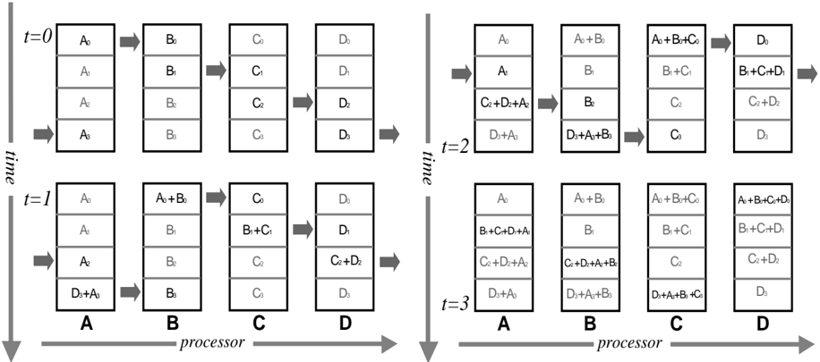/0 Figure 12: Pipelined Summing with Processors Configured in a Ring <details> <summary>Image 12 Details</summary>  ### Visual Description ## Diagram: Data Processing Across Processors Over Time ### Overview The image is a diagram illustrating a data processing pipeline across four processors (A, B, C, and D) over four time steps (t=0, t=1, t=2, t=3). Each processor holds a stack of data elements, and the diagram shows how these elements are combined and passed between processors at each time step. ### Components/Axes * **Processors (Horizontal Axis):** Labeled A, B, C, and D. Represented as vertical stacks of data elements. * **Time (Vertical Axis):** Labeled t=0, t=1, t=2, and t=3. Indicates the progression of the data processing stages. * **Data Elements:** Represented as boxes within each processor's stack. Each box contains a data element or a combination of data elements. * **Arrows:** Indicate the flow of data between processors. ### Detailed Analysis **Time t=0:** * **Processor A:** Contains data elements A0, A1, A2, and A3. * **Processor B:** Contains data elements B0, B1, B2, and B3. * **Processor C:** Contains data elements C0, C1, C2, and C3. * **Processor D:** Contains data elements D0, D1, D2, and D3. **Time t=1:** * **Processor A:** Contains data elements A0, A1, A2, and D3+A3. * **Processor B:** Contains data elements A0+B0, B1, B2, and B3. * **Processor C:** Contains data elements C0, B1+C1, C2, and C3. * **Processor D:** Contains data elements D0, D1, C2+D2, and D3. **Time t=2:** * **Processor A:** Contains data elements A0, A1, C2+D2+A2, and D3+A3. * **Processor B:** Contains data elements A0+B0, B1, B2, and D3+A3+B3. * **Processor C:** Contains data elements A0+B0+C0, B1+C1, C2, and C3. * **Processor D:** Contains data elements D0, B1+C1+D1, C2+D2, and D3. **Time t=3:** * **Processor A:** Contains data elements A0, B1+C1+D1+A0, C2+D2+A2, and D3+A3. * **Processor B:** Contains data elements A0+B0, B1, C2+D2+A2+B3, and D3+A3+B3. * **Processor C:** Contains data elements A0+B0+C0, B1+C1, C2, and D3+A3+B3+C3. * **Processor D:** Contains data elements A0+B0+C0+D0, B1+C1+D1, C2+D2, and D3. ### Key Observations * Data flows from left to right, from processor A to D. * At each time step, data elements are combined and passed to the next processor. * The data elements in processor A at time t=1 include data from processor D at time t=0. * The data elements in processor B at time t=1 include data from processor A at time t=0. * The data elements in processor C at time t=1 include data from processor B at time t=0. * The data elements in processor D at time t=1 include data from processor C at time t=0. * The data elements in processor A at time t=2 include data from processor C and D at time t=0. * The data elements in processor B at time t=2 include data from processor D at time t=0 and A at time t=1. * The data elements in processor C at time t=2 include data from processor A and B at time t=1. * The data elements in processor D at time t=2 include data from processor B and C at time t=1. * The data elements in processor A at time t=3 include data from processor B, C and D at time t=1. * The data elements in processor B at time t=3 include data from processor C and D at time t=1 and A at time t=2. * The data elements in processor C at time t=3 include data from processor A, B and D at time t=2. * The data elements in processor D at time t=3 include data from processor A, B and C at time t=2. ### Interpretation The diagram illustrates a pipelined data processing system where data is processed in stages across multiple processors. Each processor performs a specific operation on the data it receives, and the results are passed to the next processor in the pipeline. The system appears to be designed to perform a series of additions or combinations of data elements. The diagram highlights how data dependencies are managed and how the results of earlier processing stages are used in later stages. The system also appears to be designed to perform a series of additions or combinations of data elements. The diagram highlights how data dependencies are managed and how the results of earlier processing stages are used in later stages. </details> In practice, the constant factor for this algorithm on GF11 is not significantly better than the log of the number of processors because of the processor dependent computation. But this extension is important in theory because it scales better with the number of processors; it indicates that a very simple processor interconnection, a ring, is adequate for our approach to parallelizing backprop provided that processor dependent addressing is possible. ## 10.3. Improving Performance for Small Networks In general, our code is optimized for networks with large enough layers to fill up the 25 cycle pipeline. However, some neural network architectures for large applications have small layers, e.g., classification tasks with a few output units[10]. Speeding up computation on smaller layers requires minimizing the longest chain of dependent operations so that more operations can be interleaved. In the forward pass, 2 floating point operations per weight are executed. Multiplies are independent of each other, but all the additions to the net input of a destination form a linear dependency chain. This chain can be shortened by rearranging the operations so that the dependency graph forms a binary tree. To sum an array x of size N (assuming N is a power of 2 for simplicity), ``` for i = 0 step 1 to lg(n)-1 for j = 0 step (2^(i+1)) to n-1 x[j]=x[j]+x[j+2^i]; ``` The result is left in x[0]. ## 10.4. Fault Tolerance While we were developing the simulator described in this report, an effort was being made to rapidly increase the number of available processors in GF11. This meant that the hardware was relatively unstable, a situation which lead us to consider ways how the program could be made more robust. Although the machine is far more stable at the time of writing [David George, 12 personal communication] than it was during program development, there are a number of interesting measures which could make the program more fault tolerant. Since we contemplate storing huge amounts of training data in RAM (i.e., up to 1.1 GBytes) there is some possibility of changes in the stored data due to transient memory errors. In order to detect such occurrences, we would like to add checksums to the training data. Such checksums could be computed very rapidly at infrequent intervals during training. As well as facilitating fault detection, checksums would provide additional utility by allowing the program to decide whether training patterns need to be reloaded following runs of other users programs. 13 Pending a fully functioning disk I/O system, such a facility could be very useful. The large amount of memory on each processor enables us to contemplate another form of fault tolerance: weight checkpointing to memory. Every few epochs, a copy of the networks weights could be copied to one of a number of checkpoint spaces in each processor's RAM (or trading 12 David George is the manager of the GF11 project at IBM. 13 This is not always necessary, the main switch diagnostic program for GF11, for example, only clobbers memory below that used for storing training cases by our program. time against space, spread across the RAM of all processors over the switch). In the event that an error in learning is detected (e.g. by a large increase in total pattern error between epochs), one of the checkpoints in RAM could be copied back as active weights and learning restarted. This technique should make learning virtually immune to transient or intermittent hardware failures. One of the problems with distributing weight changes, rather than weights, to all processors during the update cycle is that the weights may begin to take on different values on different processors. There are two ways in which this could occur. First, an arithmetic or memory failure on a processor could change a weight. Secondly, and less obviously, the order in which weight changes are added together is different on different processors. Since the numbers are floating point with a fixed representation, this can result in different totals on different processors, i.e., floating point operations are not necessarily associative. Small differences between weights on different processors can probably be tolerated over a few training epochs, but they need to be prevented from accumulating. We propose to ensure that all processor work on more or less the same network by occasionally averaging and rebroadcasting the 'reasonable' values for each weight across processors. ## 10.5. Recurrent Networks The final goal of this work was applying backpropagation training to the problem of speech recognition using recurrent (Elman) nets. The important difference between these networks and those with a conventional, feed forward structure is that unit activation levels are copied to units in earlier layers between presentations of successive patterns in a sequence. Since a unit's previous value contributes to its input, the network can learn weights that allow it to retain useful information over time. The copying of activations between pattern presentations presents a slight difficulty for parallelization. Activations must be copied from units in the copy of the network which saw the previous Input/Output pattern in a sequence. This means that if we spread cases from sequences across processors we would have to do the costly operation of communicating activation levels across the switch. The secret in avoiding this is to repeat the method used in Witbrock's previous vectorized Elman net simulator for the Convex C-1: parallelizing across sequences instead of across cases. This means that all copying of activation happens within the processor responsible for a particular sequence. While the actual copying of activations is trivial - a small piece of microcode is constructed from a list of (from unit, to unit) pairs at microcode generation time parallelizing across cases involves a couple of extra complications. First, a processor must know when a new sequence starts within its patterns, so that it can zero out the units which receive copies of activations. This is done by keeping a flag with each pattern: 1.0 if it's the continuation of an old sequence and 0.0 if it's the start of a new sequence, and multiplying the copied activations by this flag before copying into the destination units. The second change is that one cannot rely on all processors having the same number of patterns, since sequences may differ in length. Any patterns beyond the end of the last sequence on each processor must be marked with a flag indicating that no error should be back-propagated for this pattern. Again, this is done by multiplying the error by the value of this flag. ## 11. Evaluation of Architectural Features In building our simulator and writing this report, we have had two equally important goals. The first goal was produce the fastest simulator possible on the hardware while maintaining enough flexibility to make it useful for our other research purposes. For this goal the chief measure of success is raw speed - millions of connections per second. Th e other goal was to evaluate features of an architecture which make it suitable or unsuitable for simulating connectionist networks, not just the performance of the whole package. We begin by analyzing alternative strategies for communication. The performance of the ring summing algorithm indicates the limitations of a single ring of processors with no processordependent addressing. Clearly, figure 8 indicates that this approach does not scale well with the number of processors. The Benˇ es Network allows more sophisticated communication which significantly improves performance. However, the pipelined ring summing algorithm presented in section 10.2 has the best asymptotic complexity. Given enough weights, the total time is independent of the number of processors. We conclude that for our approach to parallelizing backprop, a sophisticated communications network is not necessary, if processor-dependent addressing is available. Although SIMD control appears at first glance to be a limitation, we did not find any need for more complex control. In fact, we found that the single thread of control made code easy to design and debug. Moreover, the GF11 processor architecture matched our needs quite well. The balance of adds and multiplies inherent in the backprop algorithm allowed us to keep the floating point units busy, and the table lookup facility proved invaluable for the sigmoid calculation. However, the three-level, software-controlled memory hierarchy added to the program complexity more than any other feature of the machine. 14 How could this complexity be avoided? It could not be prevented by a hardware controlled cache because of the pattern of the sequential accesses to large arrays. It is uncertain that compiler support would help either. Simply reducing the memory capacity in order to provide a uniform access time would place unacceptable constraints on simulation size. The best solution would be to increase the number of interleaved memory banks. It is relatively easy to arrange for weights to be accessed strictly sequentially. The bandwidth would have to be increased, but the latency would not have to be decreased. In fact we found a general principle for simulating large networks: bandwidth is much more important that latency. This principle applies to computation on weights, memory accesses to weights, and inter-processor communication. Even though the processor pipeline is 25 deep, our code was naturally amenable to pipeline scheduling without any deliberate restructuring. 14 We were not alone in finding this; Yurij Baransky [personal communication] reports that the memory hierarchy has presented difficult design decisions when mapping other applications to GF11. ## 12. Conclusions This paper reports our experience in mapping the backprop algorithm onto the GF11. We feel that there are several contributions that this work makes to the enterprise of neural network simulation: We formalized the structure of the storage access patterns during the algorithm and used this model to design an efficient mapping on to a software controlled 3-level memory hierarchy. Although the fine details of this mapping are specific to GF11, the technique of accessing a subset of weights over several training examples is directly applicable to other machines, even machines with a hardware controlled cache. We measured the simulator performance empirically, and more importantly produced an analytical model of its performance. This allowed us to independently evaluate the contribution to performance on this task of the various architectural features of GF11. Finally, we showed that although GF11 was conceived with a particular application in Quantum Chromodynamics[1] in mind, the architecture is also well-suited to other applications. ## 13. Acknowledgements We would like to thank Scott Fahlman (CMU), Danny Sabbah (IBM), and Dave George (IBM) for initiating this project. We are very grateful to Dave George, Yurij Baransky, Jim Sexton, and Micky Tsao at IBM for their technical assistance and helpful advice, and to Michael Portuesi, Micky Tsao, and Michael Franzini for help shipping data and equipment between CMU and T.J. Watson. And we also thank the CMU Boltzmann group, Yurij Baransky, Guy Blelloch, Scott Fahlman, Alan Fisher, and Dean Pomerleau for their helpful comments on the presentation of this work. ## References - [1] Beetem, J., Denneau, M. and Weingarten, D., 'The GF11 Par allel Computer', IBM Technical Report 12364, December, 1986. - [2] Benes, V. 'Optimal Rearrangeable Multistage Connectin g Networks', Bell System Technical Journal, vol. 43, 1641, 1964. - [3] Blelloch, G. and Rosenberg, C.R., 'Network learning on t he Connection Machine', Proceedings of the Tenth International Joint Conference on Artificial Intelligence , Milan, Italy, 1987. - [4] Elman, J.L. Finding Structure in Time , Technical Report, Center for Research in Language, University of California, San Diego, April, 1988. - [5] Fahlman, S.E. Faster-Learning Variations on Back-Propagation: An Empirical Study , Proceedings of the 1988 Connectionist Models Summer School , Morgan Kaufman, San Mateo. 1988. - [6] Franzini, M.A., Witbrock, M.J., and Lee, K.-F., 'A Connectionist Approach to Continuous Speech Recognition', ICASSP-89: 1980 International Conference on Acoustics, Speech and Signal Processing , pp.425-8 vol.1, IEEE, Glasgow, U.K. May, 1989. - [7] Gorman, P.R. and Sejnowski, T.J. 'Learned Classificatio n of Sonar Targets Using a Massively Parallel Network', IEEE Transactions on Acoustics, Speech, and Signal Processing, Vol 36., No. 7, 1988. - [8] Hillis, W.D. and Steele, G.L., 'Data Parallel Algorithm s', Communications of the ACM , December, 1986. - [9] Lang, K.J. and Hinton, G.E., ATime-Delay Neural Network Architecture for Speech Recognition , Technical Report CMU-CS-88-152, Carnegie Mellon University, December, 1988. - [10] Lang, K.J. and Witbrock, M.J., 'Learning to Tell Two Spi rals Apart', Proceedings of the 1988 Connectionist Models Summer School , Morgan Kaufman, San Mateo. 1988. - [11] Leonard, R.G. 'A Database for Speaker-Independent Dig it Recognition', Proceedings of the ICASSP , March, 1984. - [12] Miikkulainen, R. and Dyer, M.G., A Modular Neural Network Architecture for Sequential Paraphrasing of Script-Based Stories , Technical Report UCLA-AI-8902, University of California, Los Angeles, February, 1989. - [13] Plaut, D.C., Nowlan, S.J., and Hinton, G.E. Experiments on learning by back propagation , Technical Report, Carnegie Mellon University, June, 1986. - [14] Pomerleau, D.A., 'ALVINN: An Autonomous Land Vehicle I n a Neural Network', Advances in Neural Information Processing Systems I , D.S. Touretzky, ed., Morgan Kaufman, 1989. - [15] Pomerleau, D.A., Gusciora, G.L., Touretzky, D.S., and Kung, H.T., 'Neural Network Simulation at Warp Speed: How We Got 17 Million Connections Per Second', Proceedings of IEEE International Conference on Neural Networks , 1988. - [16] Rumelhart, D.E., Hinton, H.E., and Williams, R.J. 'Lea rning Internal Representations by Error Propagation'. in Rumelhart, D.E., McClelland, J.L., eds., Parallel Distributed Processing: Explorations in the Microstructure of Cognition. Vol I., The MIT Press, Cambridge, 1986. - [17] Sejnowski, T.J. and Rosenberg, C. 'Parallel Networks t hat Learns to Pronounce English Text', Complex Systems , 1, 145-168, 1987. - [18] Zhang, X., McKenna, M., Mesirov, J., and Waltz, D. 'An Implementation of the Backpropagation Algorithm on the Connection Machine CM-2', Proceedings of Neural Information Processing Systems 1989, in press.