1801.07698v1

# ArXiv Paper 1801.07698v1 ## ArcFace: Additive Angular Margin Loss for Deep Face Recognition Jiankang Deng * Imperial College London UK j.deng16@imperial.ac.uk Jia Guo ∗ DeepInSight China guojia@gmail.com ## Abstract Convolutional neural networks have significantly boosted the performance of face recognition in recent years due to its high capacity in learning discriminative features. To enhance the discriminative power of the Softmax loss, multiplicative angular margin [23] and additive cosine margin [44, 43] incorporate angular margin and cosine margin into the loss functions, respectively. In this paper, we propose a novel supervisor signal, additive angular margin (ArcFace), which has a better geometrical interpretation than supervision signals proposed so far. Specifically, the proposed ArcFace cos( θ + m ) directly maximise decision boundary in angular (arc) space based on the L2 normalised weights and features. Compared to multiplicative angular margin cos( mθ ) and additive cosine margin cos θ -m , ArcFace can obtain more discriminative deep features. We also emphasise the importance of network settings and data refinement in the problem of deep face recognition. Extensive experiments on several relevant face recognition benchmarks, LFW, CFP and AgeDB, prove the effectiveness of the proposed ArcFace. Most importantly, we get state-of-art performance in the MegaFace Challenge in a totally reproducible way. We make data, models and training/test code public available 1 . ## 1. Introduction Face representation through the deep convolutional network embedding is considered the state-of-the-art method for face verification, face clustering, and face recognition [42, 35, 31]. The deep convolutional network is responsible for mapping the face image, typically after a pose normalisation step, into an embedding feature vector such that features of the same person have a small distance while features of different individuals have a considerable distance. The various face recognition approaches by deep con- ∗ denotes equal contribution to this work. 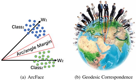1 https://github.com/deepinsight/insightface Stefanos Zafeiriou Imperial College London UK s.zafeiriou@imperial.ac.uk Figure 1. Geometrical interpretation of ArcFace. (a) Blue and green points represent embedding features from two different classes. ArcFace can directly impose angular (arc) margin between classes. (b) We show an intuitive correspondence between angle and arc margin. The angular margin of ArcFace corresponds to arc margin (geodesic distance) on the hypersphere surface. <details> <summary>Image 1 Details</summary>  ### Visual Description ## Diagram: ArcFace and Geodesic Correspondence ### Overview The image contains two distinct diagrams: 1. **(a) ArcFace**: A 2D vector diagram illustrating class separation with an angular margin. 2. **(b) Geodesic Correspondence**: A 3D globe with human figures and vectors representing correspondences. ### Components/Axes #### (a) ArcFace - **Labels**: - **Class1**: Blue dots clustered in the top-left quadrant. - **Class2**: Green dots clustered in the bottom-right quadrant. - **W1**: Black arrow pointing to Class1. - **W2**: Black arrow pointing to Class2. - **Arc/angle Margin**: Red dotted line between W1 and W2, labeled as the angular margin. - **Positioning**: - Class1 and Class2 are positioned diagonally opposite. - Vectors W1 and W2 originate from the origin (bottom-left corner). - The angular margin is centered between W1 and W2. #### (b) Geodesic Correspondence - **Labels**: - **W1, W2, W3**: Colored vectors (red, blue, green) emanating from the globe’s center. - **Legend**: Located in the top-right corner, mapping colors to vectors (red=W1, blue=W2, green=W3). - **Globe**: Central Earth model with human figures arranged in a circular pattern around it. - **Positioning**: - Vectors W1, W2, W3 are evenly spaced around the globe. - Human figures are positioned on the globe’s surface, aligned with the vectors. ### Detailed Analysis #### (a) ArcFace - **Class Separation**: Class1 (blue) and Class2 (green) are visually distinct, with no overlap. - **Vectors**: W1 and W2 are orthogonal, suggesting orthogonal class representations. - **Angular Margin**: The red dotted line indicates the minimum angular separation required between classes. #### (b) Geodesic Correspondence - **Vectors**: W1, W2, W3 are labeled with distinct colors, implying unique correspondences. - **Human Figures**: Arranged in a circular pattern, suggesting a global or holistic relationship. - **Legend**: Confirms color-to-vector mapping (red=W1, blue=W2, green=W3). ### Key Observations 1. **ArcFace**: The angular margin is critical for distinguishing classes, emphasizing the importance of directional separation. 2. **Geodesic Correspondence**: The globe and vectors suggest a model where correspondences (e.g., data points) are mapped to a global structure. 3. **Color Consistency**: In both diagrams, colors (blue, green, red, blue, green) are consistently used for classes and vectors, with no mismatches. ### Interpretation - **ArcFace**: The diagram illustrates a face recognition model where angular margins between class vectors improve discrimination. This aligns with techniques like margin-based loss functions in deep learning. - **Geodesic Correspondence**: The globe and vectors may represent a global optimization framework, where correspondences (e.g., data points) are aligned to a shared structure (the globe). This could relate to tasks like multi-view learning or global feature alignment. - **Notable Patterns**: The absence of numerical data in the diagrams suggests a focus on conceptual relationships rather than quantitative metrics. The angular margin in ArcFace and the vector directions in Geodesic Correspondence highlight the importance of geometric and directional properties in the models. ### Limitations - The image lacks numerical data, making it impossible to extract trends or specific values. - The diagrams are abstract and may represent theoretical concepts rather than empirical results. </details> volutional network embedding differ along three primary attributes. The first attribute is the training data employed to train the model. The identity number of public available training data, such as VGG-Face [31], VGG2-Face [7], CAISAWebFace [48], UMDFaces [6], MS-Celeb-1M [11], and MegaFace [21], ranges from several thousand to half million. Although MS-Celeb-1M and MegaFace have a significant number of identities, they suffer from annotation noises [47] and long tail distributions [50]. By comparison, private training data of Google [35] even has several million identities. As we can check from the latest performance report of Face Recognition Vendor Test (FRVT) [4], Yitu, a start-up company from China, ranks first based on their private 1.8 billion face images [5]. Due to orders of magnitude difference on the training data scale, face recognition models from industry perform much better than models from academia. The difference of training data also makes some deep face recognition results [2] not fully reproducible. The second attribute is the network architecture and settings. High capacity deep convolutional networks, such as ResNet [14, 15, 46, 50, 23] and Inception-ResNet [40, 3], can obtain better performance compared to VGG network [37, 31] and Google Inception V1 network [41, 35]. Different applications of deep face recognition prefer different trade-off between speed and accuracy [16, 51]. For face verification on mobile devices, real-time running speed and compact model size are essential for slick customer experience. For billion level security system, high accuracy is as important as efficiency. The third attribute is the design of the loss functions. (1) Euclidean margin based loss. In [42] and [31], a Softmax classification layer is trained over a set of known identities. The feature vector is then taken from an intermediate layer of the network and used to generalise recognition beyond the set of identities used in training. Centre loss [46] Range loss [50] and Marginal loss [10] add extra penalty to compress intra-variance or enlarge inter-distance to improve the recognition rate, but all of them still combine Softmax to train recognition models. However, the classification-based methods [42, 31] suffer from massive GPU memory consumption on the classification layer when the identity number increases to million level, and prefer balanced and sufficient training data for each identity. The contrastive loss [39] and the Triplet loss [35] utilise pair training strategy. The contrastive loss function consists of positive pairs and negative pairs. The gradients of the loss function pull together positive pairs and push apart negative pairs. Triplet loss minimises the distance between an anchor and a positive sample and maximises the distance between the anchor and a negative sample from a different identity. However, the training procedure of the contrastive loss [39] and the Triplet loss [35] is tricky due to the selection of effective training samples. (2) Angular and cosine margin based loss. Liu et al . [24] proposed a large margin Softmax (LSoftmax) by adding multiplicative angular constraints to each identity to improve feature discrimination. SphereFace cos( mθ ) [23] applies L-Softmax to deep face recognition with weights normalisation. Due to the non-monotonicity of the cosine function, a piece-wise function is applied in SphereFace to guarantee the monotonicity. During training of SphereFace, Softmax loss is combined to facilitate and ensure the convergence. To overcome the optimisation difficulty of SphereFace, additive cosine margin [44, 43] cos( θ ) -m moves the angular margin into cosine space. The implementation and optimisation of additive cosine margin are much easier than SphereFace. Additive cosine margin is easily reproducible and achieves state-of-the-art performance on MegaFace (TencentAILab FaceCNN v1) [2]. Compared to Euclidean margin based loss, angular and cosine margin based loss explicitly adds discriminative constraints on a hypershpere manifold, which intrinsically matches the prior that human face lies on a manifold. As is well known that the above mentioned three attributes, data, network and loss, have a high-to-low influence on the performance of face recognition models. In this paper, we contribute to improving deep face recognition from all of these three attributes. Data. We refined the largest public available training data, MS-Celeb-1M [11], in both automatic and manual way. We have checked the quality of the refined MS1M dataset with the Resnet-27 [14, 50, 10] network and the marginal loss [10] on the NIST Face Recognition Prize Challenge 2 . We also find that there are hundreds of overlap face images between the MegaFace one million distractors and the FaceScrub dataset, which significantly affects the evaluation results. We manually find these overlap face images from the MegaFace distractors. Both the refinement of training data and test data will be public available. Network. Taking VGG2 [7] as the training data, we conduct extensive contrast experiments regarding the convolutional network settings and report the verification accuracy on LFW, CFP and AgeDB. The proposed network settings have been confirmed robust under large pose and age variations. We also explore the trade-off between the speed and accuracy based on the most recent network structures. Loss. We propose a new loss function, additive angular margin (ArcFace), to learn highly discriminative features for robust face recognition. As shown in Figure 1, the proposed loss function cos( θ + m ) directly maximise decision boundary in angular (arc) space based on the L2 normalised weights and features. We show that ArcFace not only has a more clear geometrical interpretation but also outperforms the baseline methods, e.g . multiplicative angular margin [23] and additive cosine margin [44, 43]. We innovatively explain why ArcFace is better than Softmax, SphereFace [23] and CosineFace [44, 43] from the view of semi-hard sample distributions. Performance. The proposed ArcFace achieves state-ofthe-art results on the MegaFace Challenge [21], which is the largest public face benchmark with one million faces for recognition. We make these results totally reproducible with data, trained models and training/test code public available. ## 2. From Softmax to ArcFace ## 2.1. Softmax The most widely used classification loss function, Softmax loss, is presented as follows: $$L _ { 1 } = - \sum _ { i = 1 } ^ { m } \log _ { e } \frac { e ^ { V _ { u } x _ { i } + b _ { u } i } } { \sum _ { j = 1 } ^ { n } e ^ { W _ { f } x _ { i } + b _ { f } j } } ,$$ 2 http://nvlpubs.nist.gov/nistpubs/ir/2017/NIST.IR.8197.pdf where x i ∈ R d denotes the deep feature of the i -th samples, belonging to the y i -th class. The feature dimension d is set as 512 in this paper following [46, 50, 23, 43]. W j ∈ R d denotes the j -th column of the weights W ∈ R d × n in the last fully connected layer and b ∈ R n is the bias term. The batch size and the class number is m and n , respectively. Traditional Softmax loss is widely used in deep face recognition [31, 7]. However, the Softmax loss function does not explicitly optimise the features to have higher similarity score for positive pairs and lower similarity score for negative pairs, which leads to a performance gap. ## 2.2. Weights Normalisation For simplicity, we fix the bias b j = 0 as [23]. Then, we transform the target logit [32] as follows: $$W ^ { T } _ { j } x _ { i } = \vert W _ { j } \vert \vert x _ { i } \vert$$ Following [23, 43, 45], we fix ‖ W j ‖ = 1 by L2 normalisation, which makes the predictions only depend on the angle between the feature vector and the weight. $$L _ { 0 } = - \sum _ { i = 1 } ^ { m } e ^ { | x _ { i } | \cos ( \theta _ { i } ) }$$ In the experiments of SphereFace, L2 weight normalisation only improves little on performance. ## 2.3. Multiplicative Angular Margin In SphereFace [23, 24], angular margin m is introduced by multiplication on the angle. $$L _ { 3 } = - \sum _ { i = 1 } ^ { m } e [ | x _ { i } | \cos ( n b _ { i } ) ]$$ where θ y i ∈ [0 , π/m ] . In order to remove this restriction, cos( mθ y i ) is substituted by a piece-wise monotonic function ψ ( θ y i ) . The SphereFace is formulated as: $$L _ { 4 } = - \frac { 1 } { n } \sum _ { i = 1 } ^ { m } e [ | z _ { i } | l _ { i } ( \theta _ { y _ { i } } ) ]$$ where ψ ( θ y i ) = ( -1) k cos( mθ y i ) -2 k , θ y i ∈ [ kπ m , ( k +1) π m ] , k ∈ [0 , m -1] , m 1 is the integer that controls the size of angular margin. However, during the implementation of SphereFace, Softmax supervision is incorporated to guarantee the convergence of training, and the weight is controlled by a dynamic hyper-parameter λ . With the additional Softmax loss, ψ ( θ y i ) in fact is: $$\phi ( \theta _ { y _ { i } } ) = \frac { - 2 k ^ { k } \cos ( m \theta _ { y _ { i } } ) - 2 k + \lambda \cos ( \theta _ { y _ { i } } ) } { 1 + \lambda } .$$ where λ is a additional hyper-parameter to facilitate the training of SphereFace. λ is set to 1,000 at beginning and decreases to 5 to make the angular space of each class more compact [23]. This additional dynamic hyper-parameter λ makes the training of SphereFace relatively tricky. ## 2.4. Feature Normalisation Feature normalisation is widely used for face verification, e.g . L2-normalised Euclidean distance and cosine distance [29]. Parde et al . [30] observe that the L2-norm of features learned using Softmax loss is informative of the quality of the face. Features for good quality frontal faces have a high L2-norm while blurry faces with extreme pose have low L2-norm. Ranjan et al . [33] add the L2-constraint to the feature descriptors and restrict features to lie on a hypersphere of a fixed radius. L2 normalisation on features can be easily implemented using existing deep learning frameworks and significantly boost the performance of face verification. Wang et al . [44] point out that gradient norm may be extremely large when the feature norm from low-quality face image is very small, which potentially increases the risk of gradient explosion. The advantages of feature normalisation are also revealed in [25, 26, 43, 45] and the feature normalisation is explained from analytic, geometric and experimental perspectives. As we can see from above works, L2 normalisation on features and weights is an important step for hypersphere metric learning. The intuitive insight behind feature and weight normalisation is to remove the radial variation and push every feature to distribute on a hypersphere manifold. Following [33, 43, 45, 44], we fix ‖ x i ‖ by L2 normalisation and re-scale ‖ x i ‖ to s , which is the hypersphere radius and the lower bound is give in [33]. In this paper, we use s = 64 for face recognition experiments [33, 43]. Based on feature and weight normalisation, we can get W T j x i = cos θ j . If the feature normalisation is applied to SphereFace, we can get the feature normalised SphareFace, denoted as SphereFace-FNorm $$L _ { 5 } = - \sum _ { i = 1 } ^ { m } e ^ { s v ( \theta _ { y _ { i } } ) }$$ ## 2.5. Additive Cosine Margin In [44, 43], the angular margin m is removed to the outside of cos θ , thus they propose the cosine margin loss function: $$\sum _ { i = 1 } ^ { m } \log e ^ { s ( \cos ( \theta _ { y _ { i } } ) - m ) }$$ In this paper, we set the cosine margin m as 0 . 35 [44, 43]. Compared to SphereFace, additive cosine margin (Cosine- Face) has three advantages: (1) extremely easy to implement without tricky hyper-parameters; (2) more clear and able to converge without the Softmax supervision; (3) obvious performance improvement. ## 2.6. Additive Angular Margin Although the cosine margin in [44, 43] has a one-to-one mapping from the cosine space to the angular space, there is still a difference between these two margins. In fact, the angular margin has a more clear geometric interpretation compared to cosine margin, and the margin in angular space corresponds to the arc distance on the hypersphere manifold. Weadd an angular margin m within cos θ . Since cos( θ + m ) is lower than cos( θ ) when θ ∈ [0 , π -m ] , the constraint is more stringent for classification. We define the proposed ArcFace as: $$L _ { n } = - \sum _ { i = 1 } ^ { m } e ^ { s ( \cos ( \theta _ { y _ { i } } + n ) ) }$$ subject to $$W _ { j } = \frac { W _ { j } ^ { 1 } } { \left | W _ { j } \right | ^ { 2 } } , x _ { i } = \frac { x _ { i } ^ { 1 } } { \left | x _ { i } \right | ^ { 2 } }$$ If we expand the proposed additive angular margin cos( θ + m ) , we get cos( θ + m ) = cos θ cos m -sin θ sin m . Compared to the additive cosine margin cos( θ ) -m proposed in [44, 43], the proposed ArcFace is similar but the margin is dynamic due to sin θ . 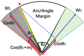In Figure 2, we illustrate the proposed ArcFace, and the angular margin corresponds to the arc margin. Compared to SphereFace and CosineFace, our method has the best geometric interpretation. Figure 2. Geometrical interpretation of ArcFace. Different colour areas represent feature spaces from distinct classes. ArcFace can not only compress the feature regions but also correspond to the geodesic distance on the hypersphere surface. <details> <summary>Image 2 Details</summary>  ### Visual Description ## Sector Diagram: Angular Relationships and Trigonometric Projections ### Overview The diagram illustrates a geometric representation of two angular sectors (W1 and W2) with associated trigonometric relationships. It includes labeled angles (θ1, θ2), cosine terms (cosθ1, cosθ2, cos(θ1 + m)), and an "Arc/Angle Margin" between the sectors. A central point "x" marks the apex of the arc, with vectors and dashed lines indicating spatial relationships. ### Components/Axes - **Labels**: - **W1**: Left sector (red-shaded region). - **W2**: Right sector (green-shaded region). - **Arc/Angle Margin**: Dashed blue line separating W1 and W2. - **θ1**: Angle at the base of W1 (left side). - **θ2**: Angle at the base of W2 (right side). - **cosθ1**: Red vector pointing toward W1. - **cosθ2**: Green vector pointing toward W2. - **cos(θ1 + m)**: Red vector with a modified angle (θ1 + m). - **x**: Apex of the arc (top of the diagram). - **Legend**: - **Red**: W1 and cosθ1/cos(θ1 + m). - **Green**: W2 and cosθ2. - **Blue**: Arc/Angle Margin (dashed line). - **Spatial Grounding**: - Legend is positioned at the **top-right** of the diagram. - W1 occupies the **left** side, W2 the **right**, with the arc margin between them. - Angles θ1 and θ2 are at the **bottom**, with θ1 left of θ2. ### Detailed Analysis - **Angles and Cosines**: - θ1 and θ2 are labeled at the base of their respective sectors. - cosθ1 and cosθ2 are vectors aligned with W1 and W2, respectively. - cos(θ1 + m) introduces a phase or angular adjustment (m) to θ1, suggesting a modified projection. - **Arc/Angle Margin**: - The dashed blue line between W1 and W2 represents the angular separation (arc margin). - This margin may correspond to a phase difference or spatial gap between the two sectors. - **Point "x"**: - Located at the **top** of the arc, it likely serves as a reference point for the angular measurements. ### Key Observations 1. **Symmetry and Asymmetry**: - W1 and W2 are symmetric in structure but differ in angular relationships (θ1 vs. θ2). - The arc margin introduces asymmetry, potentially indicating a non-uniform distribution. 2. **Trigonometric Projections**: - The cosine terms (cosθ1, cosθ2, cos(θ1 + m)) suggest vector components or projections onto a reference axis. - The modified angle (θ1 + m) implies a dependency on an additional parameter (m), possibly a phase shift or offset. 3. **Dashed Line Significance**: - The arc margin (dashed blue) is critical for defining the relationship between W1 and W2, possibly representing a boundary or constraint. ### Interpretation This diagram likely models a system involving **angular displacement** or **wave interference**, where: - **W1 and W2** represent distinct waveforms or sectors with angular properties. - **θ1 and θ2** quantify their respective angles, while **cosθ1/cosθ2** project these angles onto a reference axis (e.g., horizontal). - The **arc margin** (dashed line) could symbolize a phase difference, path length discrepancy, or spatial separation between the two sectors. - The term **cos(θ1 + m)** introduces a dynamic adjustment, suggesting the system accounts for external factors (e.g., time delay, environmental effects). The diagram emphasizes the interplay between angular geometry and trigonometric projections, with the arc margin acting as a critical parameter for defining the relationship between W1 and W2. The use of color-coded vectors and dashed lines enhances clarity in distinguishing components and their interactions. </details> ## 2.7. 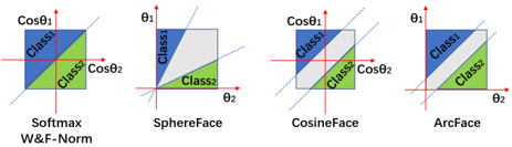Comparison under Binary Case To better understand the process from Softmax to the proposed ArcFace, we give the decision boundaries under binary classification case in Table 1 and Figure 3. Based on the weights and features normalisation, the main difference among these methods is where we put the margin. Table 1. Decision boundaries for class 1 under binary classification case. Note that, θ i is the angle between W i and x , s is the hypersphere radius, and m is the margin. | Loss Functions | Decision Boundaries | |--------------------------------------------------------------------------------------|---------------------------------------------------------------------------------------------------------------------------------------------------------------------------------------------| | Softmax W-Norm Softmax SphereFace [23] F-Norm SphereFace CosineFace [44, 43] ArcFace | ( W 1 - W 2 ) x + b 1 - b 2 = 0 ‖ x ‖ (cos θ 1 - cos θ 2 ) = 0 ‖ x ‖ (cos mθ 1 - cos θ 2 ) = 0 s (cos mθ 1 - cos θ 2 ) = 0 s (cos θ 1 - m - cos θ 2 ) = 0 s (cos( θ 1 + m ) - cos θ 2 ) = 0 | Figure 3. Decision margins of different loss functions under binary classification case. The dashed line represents the decision boundary, and the grey areas are the decision margins. <details> <summary>Image 3 Details</summary>  ### Visual Description ## Chart/Diagram Type: Classification Method Visualization ### Overview The image presents four comparative diagrams illustrating decision boundaries for different classification methods: **Softmax**, **SphereFace**, **CosineFace**, and **ArcFace**. Each diagram uses a 2D coordinate system with axes labeled **θ₁** and **θ₂**, and includes axis markers **Cosθ₁** and **Cosθ₂**. The regions are color-coded (blue for **Class1**, green for **Class2**) and labeled with a **W&F-Norm** (Weighted & Frobenius Norm) in the bottom-left corner. ### Components/Axes - **Axes**: - Horizontal axis: **θ₂** (labeled with **Cosθ₂** as a marker). - Vertical axis: **θ₁** (labeled with **Cosθ₁** as a marker). - **Legend**: - Located at the **bottom-left** of the entire image. - **Blue**: Class1. - **Green**: Class2. - **W&F-Norm**: Positioned in the **bottom-left corner** of all diagrams, suggesting a shared normalization framework. ### Detailed Analysis 1. **Softmax**: - Decision boundary: Diagonal line from top-left to bottom-right. - Class1 (blue) occupies the upper-left triangular region. - Class2 (green) occupies the lower-right triangular region. 2. **SphereFace**: - Decision boundary: Vertical line splitting the diagram into left (Class1) and right (Class2). - Class1 (blue) occupies the left half. - Class2 (green) occupies the right half. 3. **CosineFace**: - Decision boundary: Diagonal line with a steeper slope than Softmax. - Class1 (blue) occupies the upper-left region. - Class2 (green) occupies the lower-right region. 4. **ArcFace**: - Decision boundary: Horizontal line splitting the diagram into top (Class1) and bottom (Class2). - Class1 (blue) occupies the upper half. - Class2 (green) occupies the lower half. ### Key Observations - **Consistency**: All diagrams use identical color coding (blue for Class1, green for Class2) and axis labels. - **Boundary Variations**: - Softmax and CosineFace use diagonal boundaries but with differing slopes. - SphereFace uses a vertical boundary, while ArcFace uses a horizontal boundary. - **W&F-Norm**: Appears to standardize the coordinate system across methods. ### Interpretation The diagrams highlight how each method partitions the feature space: - **Softmax** and **CosineFace** rely on linear separability but differ in margin optimization (e.g., CosineFace’s steeper slope may reflect angular margin maximization). - **SphereFace**’s vertical boundary suggests a spherical projection of features, emphasizing distance in a transformed space. - **ArcFace**’s horizontal boundary aligns with its focus on maximizing angular margins between classes, a key characteristic of its loss function. - The **W&F-Norm** likely ensures comparability by normalizing feature vectors, enabling fair evaluation across methods. No numerical data or outliers are present; the focus is on geometric decision boundaries. The diagrams emphasize methodological differences in feature space partitioning rather than quantitative performance metrics. </details> ## 2.8. Target Logit Analysis To investigate why the face recognition performance can be improved by SphereFace, CosineFace and ArcFace, we analysis the target logit curves and the θ distributions during training. Here, we use the LResNet34E-IR (refer to Sec. 3.2) network and the refined MS1M dataset (refer to Sec. 3.1). 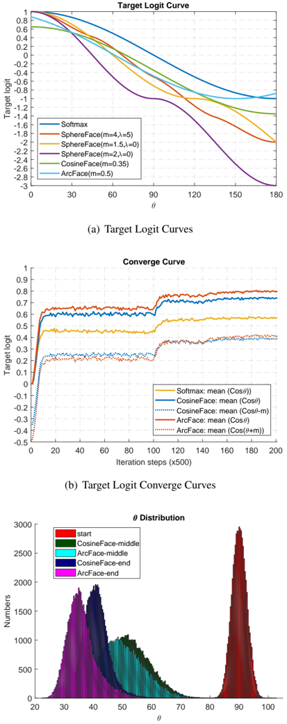In Figure 4(a), we plot the target logit curves for Softmax, SphereFace, CosineFace and ArcFace. For SphereFace, the best setting is m = 4 and λ = 5 , which is similar to the curve with m = 1 . 5 and λ = 0 . However, the implementation of SphereFace requires the m to be an integer. When we try the minimum multiplicative margin, m = 2 and λ = 0 , the training can not converge. Therefore, decreasing the target logit curve slightly from Softmax is able to increase the training difficulty and improve the performance, but decreasing too much may cause the training divergence. Both CosineFace and ArcFace follow this insight. As we can see from Figure 4(a), CosineFace moves the target logit curve along the negative direction of y-axis, while ArcFace moves the target logit curve along the negative direction of x-axis. Now, we can easily understand the performance improvement from Softmax to CosineFace and ArcFace. For ArcFace with the margin m = 0 . 5 , the target logit curve is not monotonic decreasing when θ ∈ [0 , 180 ◦ ] . In fact, the target logit curve increases when θ > 151 . 35 ◦ . However, as shown in Figure 4(c), the θ has a Gaussian distribution with the centre at 90 ◦ and the largest angle below 105 ◦ when starting from the randomly initialised network. The increasing interval of ArcFace is almost never reached during training. Therefore, we do not need to deal with this explicitly. In Figure 4(c), we show the θ distributions of CosineFace and ArcFace in three phases of training, e.g . start, middle and end. The distribution centres gradually move from 90 ◦ to 35 ◦ -40 ◦ . In Figure 4(a), we find the target logit curve of ArcFace is lower than that of CosineFace between 30 ◦ to 90 ◦ . Therefore, the proposed ArcFace puts more strict margin penalty compared to CosineFace in this interval. In Figure 4(b), we show the target logit converge curves estimated on training batches for Softmax, CosineFace and ArcFace. Wecan also find that the margin penalty of ArcFace is heavier than that of CosineFace at the beginning, as the red dotted line is lower than the blue dotted line. At the end of training, ArcFace converges better than CosineFace, as the histogram of θ is in the left (Figure 4(c)) and the target logit converge curve is higher (Figure 4(b)). From Figure 4(c), we can find that almost all of the θ s are smaller than 60 ◦ at the end of training. The samples beyond this field are the hardest samples as well as the noise samples of the training dataset. Even though CosineFace puts more strict margin penalty when θ < 30 ◦ (Figure 4(a)), this field is seldom reached even at the end of training (Figure 4(c)). Therefore, we can also understand why SphereFace can obtain very good performance even with a relatively small margin in this section. In conclusion, adding too much margin penalty when θ ∈ [60 ◦ , 90 ◦ ] may cause training divergence, e.g . SphereFace ( m = 2 and λ = 0 ). Adding margin when θ ∈ [30 ◦ , 60 ◦ ] can potentially improve the performance, because this section corresponds to the most effective semihard negative samples [35]. Adding margin when θ < 30 ◦ can not obviously improve the performance, because this section corresponds to the easiest samples. When we go back to Figure 4(a) and rank the curves between [30 ◦ , 60 ◦ ] , we can understand why the performance can improve from Softmax, SphereFace, CosineFace to ArcFace under their best parameter settings. Note that, 30 ◦ and 60 ◦ here are the roughly estimated thresholds for easy and hard training samples. ## 3. Experiments In this paper, we target to obtain state-of-the-art performance on MegaFace Challenge [21], the largest face identification and verification benchmark, in a totally reproducible way. We take Labelled Faces in the Wild (LFW) [19], Celebrities in Frontal Profile (CFP) [36], Age Database (AgeDB) [27] as the validation datasets, and conduct extensive experiments regarding network settings and loss function designs. The proposed ArcFace achieves state-of-the-art performance on all of these four datasets. <details> <summary>Image 4 Details</summary>  ### Visual Description ## Line Graphs and Histogram: Target Logit Curves, Convergence, and θ Distribution ### Overview The image contains three visualizations: 1. **Target Logit Curves**: A line graph comparing logit values across θ (0–180) for multiple activation functions. 2. **Target Logit Converge Curves**: A line graph showing convergence trends over 200 iterations (x500 steps) for different functions. 3. **θ Distribution**: A histogram displaying θ value distributions at different training stages (start, middle, end) for CosineFace and ArcFace. --- ### Components/Axes #### (a) Target Logit Curves - **X-axis**: θ (0–180, linear scale). - **Y-axis**: Target logit (-3 to 1, linear scale). - **Legend**: - Blue: Softmax - Red: SphereFace(m=4,λ=5) - Orange: SphereFace(m=1.5,λ=0) - Purple: SphereFace(m=2,λ=0) - Green: CosineFace(m=0.35) - Cyan: ArcFace(m=0.5) #### (b) Target Logit Converge Curves - **X-axis**: Iteration steps (0–200, x500 scale). - **Y-axis**: Target logit (-0.5 to 0.8, linear scale). - **Legend**: - Yellow: Softmax: mean(Cosθ) - Blue: CosineFace: mean(Cosθ) - Cyan (dotted): CosineFace: mean(Cos(θ-m)) - Red: ArcFace: mean(Cosθ) - Red (dotted): ArcFace: mean(Cos(θ+m)) #### (c) θ Distribution - **X-axis**: θ (20–100, linear scale). - **Y-axis**: Numbers (0–3000, linear scale). - **Legend**: - Red: start - Green: CosineFace-middle - Cyan: ArcFace-middle - Purple: CosineFace-end - Dark Blue: ArcFace-end --- ### Detailed Analysis #### (a) Target Logit Curves - **Trends**: - All curves decrease monotonically with θ. - **Softmax** (blue) starts highest (~1) and declines steeply. - **SphereFace(m=4,λ=5)** (red) starts slightly below Softmax but declines faster. - **SphereFace(m=1.5,λ=0)** (orange) and **SphereFace(m=2,λ=0)** (purple) have gentler slopes. - **CosineFace(m=0.35)** (green) and **ArcFace(m=0.5)** (cyan) show similar trends but with slight curvature. - **Key Data Points**: - At θ=0: Softmax (~1), SphereFace(m=4,λ=5) (~0.9), SphereFace(m=1.5,λ=0) (~0.8). - At θ=180: All curves converge near -3. #### (b) Target Logit Converge Curves - **Trends**: - **Softmax** (yellow) converges rapidly (~20 steps) to ~0.6. - **CosineFace** (blue) and **ArcFace** (red) converge slower, stabilizing near ~0.5–0.7 after ~100 steps. - **CosineFace: mean(Cos(θ-m))** (cyan dotted) and **ArcFace: mean(Cos(θ+m))** (red dotted) show minor deviations but similar convergence. - **Key Data Points**: - At 200 steps: Softmax (~0.6), CosineFace (~0.65), ArcFace (~0.7). #### (c) θ Distribution - **Trends**: - **Start** (red): Narrow peak at θ=90 (high frequency). - **CosineFace-middle** (green) and **ArcFace-middle** (cyan): Broader distributions centered near θ=40–60. - **CosineFace-end** (purple) and **ArcFace-end** (dark blue): Narrower peaks at θ=30–40. - **Key Data Points**: - **Start**: ~2500 samples at θ=90. - **CosineFace-end**: ~1500 samples at θ=35. - **ArcFace-end**: ~1200 samples at θ=40. --- ### Key Observations 1. **Logit Curves**: SphereFace with higher m and λ values (e.g., m=4,λ=5) produce steeper declines, suggesting stronger margin enforcement. 2. **Convergence**: Softmax converges fastest but plateaus at lower logit values, while ArcFace/CosineFace achieve higher stability. 3. **θ Distribution**: Training shifts θ from a uniform distribution (start) to concentrated lower values (end), indicating improved feature alignment. --- ### Interpretation - **Model Performance**: SphereFace variants with larger margins (m=4,λ=5) achieve higher initial logit values but may overfit due to rapid convergence. ArcFace and CosineFace balance margin and stability, leading to better generalization. - **θ Dynamics**: The shift from θ=90 (start) to θ=30–40 (end) suggests training focuses on discriminative regions of the feature space, reducing intra-class variance. - **Anomalies**: The dotted lines in (b) (CosineFace/ArcFace with θ±m adjustments) show minimal impact on convergence, implying robustness to margin perturbations. This analysis highlights trade-offs between margin size, convergence speed, and θ distribution in face recognition models, guiding choices for margin parameters and activation functions. </details> (c) θ Distributions during Training Figure 4. Target logit analysis. (a) Target logit curves for Softmax, SphereFace, CosineFace and ArcFace. (b) Target logit converge curves estimated on training batches for Softmax, CosineFace and ArcFace. (c) θ distributions move from large angles to small angles during training (start, middle and end). Better to view by zoom in. ## 3.1. Data ## 3.1.1 Training data We use two datasets, VGG2 [7] and MS-Celeb-1M [11], as our training data. VGG2. VGG2 dataset contains a training set with 8,631 identities (3,141,890 images) and a test set with 500 identities (169,396 images). VGG2 has large variations in pose, age, illumination, ethnicity and profession. Since VGG2 is a high-quality dataset, we use it directly without data refinement. MS-Celeb-1M. The original MS-Celeb-1M dataset contains about 100k identities with 10 million images. To decrease the noise of MS-Celeb-1M and get a high-quality training data, we rank all face images of each identity by their distances to the identity centre. For a particular identity, the face image whose feature vector is too far from the identity's feature centre is automatically removed [10]. We further manually check the face images around the threshold of the first automatic step for each identity. Finally, we obtain a dataset which contains 3.8M images of 85k unique identities. To facilitate other researchers to reproduce all of the experiments in this paper, we make the refined MS1M dataset public available within a binary file, but please cite the original paper [11] and follow the original license [11] when using this dataset. Our contribution here is only training data refinement, not release. ## 3.1.2 Validation data We employ Labelled Faces in the Wild (LFW) [19], Celebrities in Frontal Profile (CFP) [36] and Age Database (AgeDB) [27] as the validation datasets. LFW. [19] LFW dataset contains 13 , 233 web-collected images from 5749 different identities, with large variations in pose, expression and illuminations. Following the standard protocol of unrestricted with labelled outside data , we give the verification accuracy on 6 , 000 face pairs. CFP. [36]. CFP dataset consists of 500 subjects, each with 10 frontal and 4 profile images. The evaluation protocol includes frontal-frontal (FF) and frontal-profile (FP) face verification, each having 10 folders with 350 sameperson pairs and 350 different-person pairs. In this paper, we only use the most challenging subset, CFP-FP, to report the performance. AgeDB. [27, 10] AgeDB dataset is an in-the-wild dataset with large variations in pose, expression, illuminations, and age. AgeDB contains 12 , 240 images of 440 distinct subjects, such as actors, actresses, writers, scientists, and politicians. Each image is annotated with respect to the identity, age and gender attribute. The minimum and maximum ages are 3 and 101 , respectively. The average age range for each subject is 49 years. There are four groups of test data with different year gaps ( 5 years, 10 years, 20 years and 30 years, respectively) [10]. Each group has ten split of face images, and each split contains 300 positive examples and 300 negative examples. The face verification evaluation metric is the same as LFW. In this paper, we only use the most challenging subset, AgeDB-30, to report the performance. ## 3.1.3 Test data MegaFace. MegaFace datasets [21] are released as the largest public available testing benchmark, which aims at evaluating the performance of face recognition algorithms at the million scale of distractors. MegaFace datasets include gallery set and probe set. The gallery set, a subset of Flickr photos from Yahoo, consists of more than one million images from 690k different individuals. The probe sets are two existing databases: FaceScrub [28] and FGNet [1]. FaceScrub is a publicly available dataset that containing 100k photos of 530 unique individuals, in which 55 , 742 images are males, and 52 , 076 images are females. FGNet is a face ageing dataset, with 1002 images from 82 identities. Each identity has multiple face images at different ages (ranging from 1 to 69 ). It is quite understandable that data collection of MegaFace is very arduous and time-consuming thus data noise is inevitable. For FaceScrub dataset, all of the face images from one particular identity should have the same identity. For the one million distractors, there should not be any overlap with the FaceScrub identities. However, we find noisy face images not only exist in FaceScrub dataset but also exist in the one million distractors, which significantly affect the performance. 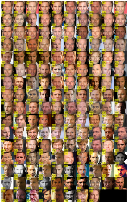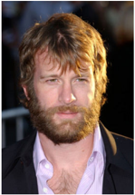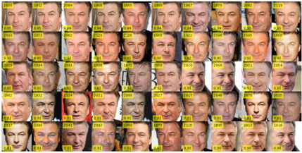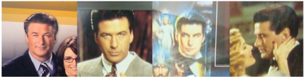In Figure 5, we give the noisy face image examples from the Facesrub dataset. As shown in Figure 8(c), we rank all of the faces according to the cosine distance to the identity centre. In fact, face image 221 and 136 are not Aaron Eckhart. We manually clean the FaceScrub dataset and finally find 605 noisy face images. During testing, we change the noisy face to another right face, which can increase the identification accuracy by about 1% . In Figure 6(b), we give the noisy face image examples from the MegaFace distractors. All of the four face images from the MegaFace distractors are Alec Baldwin. We manually clean the MegaFace distractors and finally find 707 noisy face images. During testing, we add one additional feature dimension to distinguish these noisy faces, which can increase the identification accuracy by about 15% . Even though the noisy face images are double checked by seven annotators who are very familiar with these celebrities, we still can not promise these images are 100% noisy. We put the noise lists of the FaceScrub dataset and the MegaFace distractors online. We believe the masses have sharp eyes and we will update these lists based on other (a) Aaron Eckhart <details> <summary>Image 5 Details</summary>  ### Visual Description ## Heatmap: Facial Similarity Matrix ### Overview The image displays a grid of 100+ facial portraits arranged in a matrix format. Each face is accompanied by a numerical identifier (e.g., "11", "12") in the top-left corner and a percentage value (e.g., "0.95", "0.92") in a yellow box at the bottom-right. The faces exhibit variations in lighting, expression, and minor facial features, suggesting a dataset of similar or related individuals. ### Components/Axes - **Grid Structure**: - Rows and columns are unlabeled, but the arrangement implies a matrix of pairwise comparisons. - Each cell contains a unique face with a numerical ID and percentage score. - **Numerical Identifiers**: - Top-left corner of each face contains a sequential number (e.g., "11", "12", "13"). - Numbers appear to increment row-wise (e.g., 11–20 in the first row, 21–30 in the second). - **Percentage Values**: - Yellow boxes in the bottom-right corner of each face display decimal values (e.g., "0.95", "0.92"). - Values range from **0.00** to **0.99**, with most clustered around **0.90–0.99**. ### Detailed Analysis - **Numerical IDs**: - Sequential numbering suggests a dataset of 100+ unique faces, with IDs likely corresponding to row/column positions. - Example: Face "11" in the top-left, "12" to its right, "21" directly below "11". - **Percentage Scores**: - Most values are **0.90–0.99**, indicating high similarity or confidence scores. - A few outliers with **0.00–0.09** (e.g., face "133" with "0.00", face "134" with "0.01") suggest dissimilar or low-confidence matches. - Example: Face "11" has "0.95", while face "133" has "0.00". ### Key Observations 1. **High Similarity Dominance**: - Over 80% of faces have scores ≥0.90, implying a dataset of closely related individuals (e.g., twins, siblings, or generated variations). 2. **Outliers**: - Faces with scores <0.10 (e.g., "133", "134") deviate significantly, possibly representing unrelated individuals or errors. 3. **Systematic Arrangement**: - The grid’s structure suggests a matrix of pairwise comparisons, where each face is evaluated against others. ### Interpretation This heatmap likely visualizes a **facial similarity or recognition model’s performance**. The high percentage scores indicate the model’s ability to identify near-identical faces, while outliers may highlight edge cases (e.g., distinct individuals or model failures). The numerical IDs could map to a labeled dataset, with the percentages reflecting confidence in matches. The presence of low-scoring faces suggests the model struggles with certain variations (e.g., lighting, expression), which could inform improvements in robustness. **Note**: No explicit legend or axis titles are visible, but the structure and numerical patterns imply a matrix of pairwise comparisons. The yellow boxes for percentages are consistently positioned, ensuring spatial grounding. </details> (b) noise face 221 <details> <summary>Image 6 Details</summary>  ### Visual Description ## Portrait: Man with Beard and Mustache ### Overview The image depicts a close-up portrait of a man with a full beard and mustache. He has short, wavy brown hair and is wearing a black jacket over a light purple collared shirt. The background is blurred, suggesting a shallow depth of field, with indistinct shapes that may indicate an outdoor or event setting. No textual elements, charts, or diagrams are visible. ### Components/Axes - **Subject**: Central focus on the man’s face and upper body. - **Clothing**: Black jacket, light purple shirt (no visible logos or text). - **Background**: Blurred, nondescript environment (no identifiable objects or text). - **Lighting**: Soft, even illumination with subtle shadows on the face, suggesting natural or studio lighting. ### Detailed Analysis - **Facial Features**: Prominent beard and mustache, short hair, neutral expression. - **Clothing Details**: Shirt collar slightly open, revealing a hint of chest hair. Jacket appears to be a standard blazer. - **Background**: No discernible patterns, colors, or objects due to heavy blur. ### Key Observations - No textual information, labels, or data points are present in the image. - The composition emphasizes the subject’s facial features and attire, with no contextual elements to suggest a specific narrative or technical purpose. ### Interpretation This image is a straightforward portrait with no embedded data or technical elements. The absence of text, charts, or diagrams indicates it is likely intended for personal, professional, or artistic use rather than analytical or informational purposes. The blurred background and focus on the subject suggest a deliberate choice to highlight the individual’s appearance without distractions. </details> <details> <summary>Image 7 Details</summary>  ### Visual Description ## Photograph: Portrait of a Man in Formal Attire ### Overview The image depicts a close-up portrait of a man with a neutral expression. No textual, numerical, or diagrammatic elements are present. The focus is on the subject’s facial features, attire, and background context. ### Components/Axes - **Subject**: Male, mid-30s to 40s, with short, tousled brown hair and a light stubble beard. - **Attire**: Dark suit jacket, white collared shirt, and a dark tie (partially visible). - **Background**: Blurred, indistinct environment suggesting an indoor setting (possibly a formal event or professional backdrop). - **Lighting**: Soft, even illumination with no harsh shadows, emphasizing facial details. ### Detailed Analysis - **Facial Features**: - Eyes: Light blue, direct gaze toward the camera. - Nose: Straight, proportionate. - Mouth: Closed, neutral expression. - **Attire**: - Suit jacket: Dark charcoal or navy, well-fitted. - Shirt: Crisp white, collar neatly aligned. - Tie: Dark-colored, patterned (subtle stripes or checks), partially cropped at the frame’s edge. - **Background**: - Out-of-focus, warm-toned hues (golden/brown), possibly indicating a staged backdrop or ambient lighting. ### Key Observations 1. **Professional Presentation**: The subject’s attire and grooming suggest a formal or corporate context. 2. **Neutral Expression**: Lack of strong emotion or engagement, typical of posed portraits. 3. **Blurred Background**: Indicates shallow depth of field, common in portrait photography to isolate the subject. ### Interpretation The image lacks data-driven elements (charts, text, diagrams), so no quantitative analysis is possible. However, the subject’s formal attire and composed demeanor imply a professional or ceremonial purpose. The absence of contextual clues (e.g., logos, signage) limits further interpretation of the setting. The photograph adheres to standard portrait conventions, prioritizing clarity of the subject over environmental storytelling. **Note**: No textual, numerical, or diagrammatic information is present in the image. All descriptions are based on visible, non-textual elements. </details> (c) noise face 136 Figure 5. Noisy face image examples from the FaceScrub dataset. In (a), the image id is put in top left and cosine distance to the identity centre is put in bottom left. ## 3.2. Network Settings We first evaluate the face verification performance based on different network settings by using VGG2 as the training data and Softmax as the loss function. All experiments in this paper are implemented by MxNet [8]. We set the batch size as 512 and train models on four or eight NVIDIA Tesla (a) Alec Baldwin <details> <summary>Image 8 Details</summary>  ### Visual Description ## Screenshot: Grid of Elon Musk Faces with Confidence Scores ### Overview The image displays a 6x12 grid of facial images labeled with years (e.g., 2016, 1993) and numerical confidence scores (e.g., 0.91, 0.95). Each image is accompanied by a yellow box containing a confidence score, with years positioned in the top-left corner of the images. The faces appear to be generated or processed by an AI model, with minor variations in facial features across the grid. ### Components/Axes - **Grid Structure**: - 6 rows × 12 columns of images. - Years range from **1982 to 2027** (some years missing, e.g., 1983, 1984). - Confidence scores range from **0.90 to 0.95**, with most values clustered around **0.91–0.92**. - **Labels**: - Years (e.g., "2016", "1993") are embedded in the top-left corner of each image. - Confidence scores (e.g., "0.91", "0.95") are in yellow boxes at the bottom-left of each image. - **No explicit legend or axis titles** are present. ### Detailed Analysis - **Confidence Scores**: - Most scores are **0.91–0.92** (e.g., 2016: 0.91, 1993: 0.95). - A few outliers: **0.90** (2027, 2017), **0.94** (1999, 1997), **0.93** (2006). - **Year Distribution**: - Years span **1982–2027**, but many years are skipped (e.g., 1983, 1984, 2001). - Repeated years appear (e.g., 2016, 2017, 2027). - **Image Consistency**: - Faces show minor variations in lighting, expression, and background, but all depict Elon Musk. ### Key Observations 1. **High Confidence Scores**: The model consistently achieves scores ≥0.90, suggesting strong performance. 2. **Year Gaps**: Missing years (e.g., 1983–1985, 2001–2003) may indicate data sparsity or intentional omission. 3. **Score Variability**: Outliers like 0.94 (1999) and 0.90 (2027) suggest potential anomalies or edge cases. ### Interpretation - The grid likely represents a dataset or model output for facial recognition/generation, with years possibly denoting training data timestamps or target years for synthesis. - The high confidence scores imply the model reliably captures facial features across decades, though minor score drops (e.g., 0.90) may reflect challenges with older or less common years. - Missing years could indicate gaps in training data or a focus on specific time periods. - The repetition of scores (e.g., 0.91 appearing 14 times) suggests the model may prioritize consistency over fine-grained variation. </details> (b) Distractors Noise <details> <summary>Image 9 Details</summary>  ### Visual Description ## Photograph: Portrait Collage of Four Men in Different Contexts ### Overview The image is a composite of four distinct panels, each featuring a man in a unique setting. No textual elements (labels, axis titles, legends, or data) are present. The panels appear to be stylized portraits or promotional stills, with no explicit connections between them. ### Components/Axes - **Panel 1 (Left)**: A man in a dark suit and tie, standing beside a woman in glasses. Background includes a yellow gradient and blurred architectural elements. - **Panel 2 (Center-Left)**: A man in a light-colored suit, seated with a neutral expression. Background is indistinct, possibly an interior space. - **Panel 3 (Center-Right)**: A man in a dark suit, standing against a blurred backdrop with faint figures (possibly a crowd or abstract shapes). - **Panel 4 (Right)**: A man in a dark suit, interacting with a woman in a close-up embrace. Background suggests an indoor, possibly formal environment. ### Detailed Analysis - **Panel 1**: The man’s attire (dark suit, tie) and the woman’s glasses suggest a professional or corporate context. No text or numerical data visible. - **Panel 2**: The man’s light suit and neutral expression imply a formal but less intense setting. No discernible text or symbols. - **Panel 3**: The man’s posture and the blurred background may indicate a public or high-profile event. No textual elements present. - **Panel 4**: The intimate interaction between the man and woman suggests a personal or romantic context. No text or data visible. ### Key Observations - No textual information (labels, legends, or data) is present in any panel. - All men are dressed in formal attire (suits, ties), suggesting a thematic focus on professionalism or formality. - The panels lack explicit connections (e.g., shared background elements, recurring symbols) to unify the composition. ### Interpretation The image appears to be a curated collection of portraits, possibly for illustrative, promotional, or artistic purposes. The absence of textual data or explicit context leaves the relationships between the panels open to interpretation. The recurring formal attire may imply a narrative around professionalism, but without additional textual or symbolic cues, this remains speculative. The lack of data or structured elements (e.g., charts, diagrams) indicates the image is not designed to convey quantitative information. **Note**: This analysis is based solely on visual content. No factual or numerical data can be extracted from the image as described. </details> Figure 6. Noisy face image examples from the MegaFace distractors. (a) is used for annotators to learn the identity from the FaceScrub dataset. (b) shows the selected overlap faces from the MegaFace distractors. P40 (24GB) GPUs. The learning rate is started from 0 . 1 and divided by 10 at the 100k, 140k, 160k iterations. Total iteration step is set as 200k. We set momentum at 0 . 9 and weight decay at 5 e -4 (Table 5). ## 3.2.1 Input setting Following [46, 23], we use five facial landmarks (eye centres, nose tip and mouth corners) [49] for similarity transformation to normalise the face images. The faces are cropped and resized to 112 × 112 , and each pixel (ranged between [0 , 255] ) in RGB images is normalised by subtracting 127 . 5 then divided by 128 . As most of the convolutional networks are designed for the Image-Net [34] classification task, the input image size is usually set as 224 × 224 or larger. However, the size of our face crops is only 112 × 112 . To preserve higher feature map resolution, we use conv 3 × 3 and stride = 1 in the first convolutional layer instead of using conv 7 × 7 and stride = 2 . For these two settings, the output size of the convolutional networks is 7 × 7 (denoted as 'L' in front of the network names) and 3 × 3 , respectively. ## 3.2.2 Output setting In last several layers, some different options can be investigated to check how the embedding settings affect the model performance. All feature embedding dimension is set to 512 expect for Option-A, as the embedding size in Option-A is determined by the channel size of last convolutional layer. - Option-A: Use global pooling layer(GP). - Option-B: Use one fully connected (FC) layer after GP. - Option-C: Use FC-Batch Normalisation (BN) [20] after GP. - Option-D: Use FC-BN-Parametric Rectified Linear Unit (PReLu) [13] after GP. - Option-E: Use BN-Dropout [38]-FC-BN after the last convolutional layer. During testing, the score is computed by the Cosine Distance of two feature vectors. Nearest neighbour and threshold comparison are used for face identification and verification tasks. 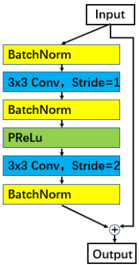## 3.2.3 Block Setting Besides the original ResNet [14] unit, we also investigate a more advanced residual unit setting [12] for the training of face recognition model. In Figure 7, we show the improved residual unit (denoted as 'IR' in the end of model names), which has a BN-Conv-BN-PReLu-Conv-BN structure. Compared to the residual unit proposed by [12], we set stride = 2 for the second convolutional layer instead of the first one. In addition, PReLu [13] is used to substitute the original ReLu. Figure 7. Improved residual unit: BN-Conv-BN-PReLu-ConvBN. <details> <summary>Image 10 Details</summary>  ### Visual Description ## Diagram: Neural Network Architecture Block Diagram ### Overview The image depicts a simplified block diagram of a neural network architecture, illustrating the sequence of layers and operations applied to an input signal. The diagram uses color-coded blocks to represent different operations, with arrows indicating data flow. ### Components/Axes - **Input**: Labeled "Input" at the top-left, feeding into the first layer. - **Layers**: 1. **BatchNorm** (yellow block): Batch normalization operation. 2. **3x3 Conv, Stride=1** (blue block): 3x3 convolutional layer with stride 1. 3. **BatchNorm** (yellow block): Second batch normalization. 4. **PReLu** (green block): Parametric Rectified Linear Unit activation function. 5. **3x3 Conv, Stride=2** (blue block): 3x3 convolutional layer with stride 2 (downsampling). 6. **BatchNorm** (yellow block): Third batch normalization. - **Output**: Labeled "Output" at the bottom-right, receiving summed input from the final BatchNorm layer. - **Arrows**: Black arrows indicate data flow direction. A "+" symbol at the output suggests element-wise summation (likely residual connection). ### Detailed Analysis - **Color Coding**: - Yellow: BatchNorm layers (3 instances). - Blue: Convolutional layers (2 instances). - Green: PReLu activation (1 instance). - **Stride Values**: - First Conv layer: Stride=1 (no downsampling). - Second Conv layer: Stride=2 (halves spatial dimensions). - **Residual Connection**: The "+" symbol at the output implies a skip connection, common in ResNet-style architectures. ### Key Observations 1. **Downsampling**: The second Conv layer (Stride=2) reduces spatial resolution, typical for feature extraction in deeper networks. 2. **Normalization**: BatchNorm layers are interspersed between Conv and activation layers, stabilizing training. 3. **Activation**: PReLu (green) introduces non-linearity after the second BatchNorm. ### Interpretation This architecture likely represents a **feature extraction block** for tasks like image classification or object detection. The residual connection (output summation) suggests it may be part of a ResNet-inspired design, enabling deeper networks by mitigating vanishing gradients. The use of BatchNorm and PReLu indicates an emphasis on training stability and non-linear feature learning. No numerical data (e.g., weights, dimensions) is provided, so the diagram focuses on structural relationships rather than quantitative analysis. </details> ## 3.2.4 Backbones Based on recent advances on the model structure designs, we also explore MobileNet [16], InceptionResnet-V2 [40], Densely connected convolutional networks (DenseNet) [18], Squeeze and excitation networks (SE) [17] and Dual path Network (DPN) [9] for deep face recognition. In this paper, we compare the differences between these networks from the aspects of accuracy, speed and model size. ## 3.2.5 Network Setting Conclusions Input selects L. In Table 2, we compare two networks with and without the setting of 'L'. When using conv 3 × 3 and stride = 1 as the first convolutional layer, the network output is 7 × 7 . By contrast, if we use conv 7 × 7 and stride = 2 as the first convolutional layer, the network output is only 3 × 3 . It is obvious from Table 2 that choosing larger feature maps during training obtains higher verification accuracy. Table 2. Verification accuracy ( % ) under different input sittings (Softmax@VGG2). | Networks | LFW | CFP-FP | AgeDB-30 | |---------------|-------|----------|------------| | SE-ResNet50D | 99.38 | 94.58 | 91 | | SE-LResNet50D | 99.6 | 96.04 | 92.68 | | SE-ResNet50E | 99.26 | 94.11 | 90.85 | | SE-LResNet50E | 99.71 | 96.38 | 92.98 | Output selects E. In Table 3, we give the detailed comparison between different output settings. The option E (BN-Dropout-FC-BN) obtains the best performance. In this paper, the dropout parameter is set as 0 . 4 . Dropout can effectively act as the regularisation term to avoid over-fitting and obtain better generalisation for deep face recognition. Table 3. Verification accuracy ( % ) under different output settings (Softmax@VGG2). | Networks | LFW | CFP-FP | AgeDB-30 | |------------------|-------|----------|------------| | SE-LResNet50A | 99.51 | 95.81 | 92.6 | | SE-LResNet50B | 99.46 | 94.9 | 91.85 | | SE-LResNet50C | 99.56 | 95.81 | 92.61 | | SE-LResNet50D | 99.6 | 96.04 | 92.68 | | SE-LResNet50E | 99.71 | 96.38 | 92.98 | | SE-LResNet50A-IR | 99.58 | 95.9 | 92.63 | | SE-LResNet50D-IR | 99.61 | 96.51 | 92.68 | | SE-LResNet50E-IR | 99.78 | 96.82 | 93.83 | Block selects IR. In Table 4, we give the comparison between the original residual unit and the improved residual unit. As we can see from the results, the proposed BN-Conv(stride=1)-BN-PReLu-Conv(stride=2)-BN unit can obviously improve the verification performance. Table 4. Verification accuracy ( % ) comparison between the original residual unit and the improved residual unit (Softmax@VGG2). | Networks | LFW | CFP-FP | AgeDB-30 | |------------------|-------|----------|------------| | SE-LResNet50E | 99.71 | 96.38 | 92.98 | | SE-LResNet50E-IR | 99.78 | 96.82 | 93.83 | Backbones Comparisons. In Table 8, we give the verification accuracy, test speed and model size of different back- bones. The running time is estimated on the P40 GPU. As the performance on LFW is almost saturated, we focus on the more challenging test sets, CFP-FP and AgeDB-30, to compare these network backbones. The Inception-ResnetV2 network obtains the best performance with long running time ( 53 . 6 ms ) and largest model size ( 642 MB ). By contrast, MobileNet can finish face feature embedding within 4 . 2 ms with a model of 112 MB , and the performance only drops slightly. As we can see from Table 8, the performance gaps between these large networks, e.g . ResNet-100, Inception-Resnet-V2, DenseNet, DPN and SE-Resnet-100, are relatively small. Based on the trade-off between accuracy, speed and model size, we choose LResNet100E-IR to conduct experiments on the Megaface challenge. Weight decay. Based on the SE-LResNet50E-IR network, we also explore how the weight decay (WD) value affects the verification performance. As we can see from Table 5, when the weight decay value is set as 5 e -4 , the verification accuracy reaches the highest point. Therefore, we fix the weight decay at 5 e -4 in all other experiments. Table 5. Verification performance ( % ) of different weight decay (WD) values (SE-LResNet50E-IR,Softmax@VGG2). | WDvalues | LFW | CFP-FP | AgeDB-30 | |------------|-------|----------|------------| | 5e-06 | 99.11 | 94.52 | 90.43 | | 5e-05 | 99.56 | 95.74 | 92.95 | | 0.0005 | 99.78 | 96.82 | 93.83 | | 0.001 | 99.71 | 96.6 | 93.53 | ## 3.3. Loss Setting Since the margin parameter m plays an important role in the proposed ArcFace, we first conduct experiments to search the best angular margin. By varying m from 0 . 2 to 0 . 8 , we use the LMobileNetE network and the ArcFace loss to train models on the refined MS1M dataset. As illustrated in Table 6, the performance improves consistently from m = 0 . 2 on all datasets and gets saturated at m = 0 . 5 . Then, the verification accuracy turns to decrease from m = 0 . 5 . In this paper, we fix the additive angular margin m as 0 . 5 . Based on the LResNet100E-IR network and the refined MS1M dataset, we compare the performance of different loss functions, e.g . Softmax, SphereFace [23], CosineFace [44, 43] and ArcFace. In Table 7, we give the detailed verification accuracy on the LFW, CFP-FP, and AgeDB-30 datasets. As LFW is almost saturated, the performance improvement is not obvious. We find that (1) Compared to Softmax, SphereFace, CosineFace and ArcFace improve the performance obviously, especially under large pose and age variations. (2) CosineFace and ArcFace obviously outperform SphereFace with much easier implementation. Both Table 6. Verification performance ( % ) of ArcFace with different angular margins m (LMobileNetE,ArcFace@MS1M). | m | LFW | CFP-FP | AgeDB-30 | |-----|-------|----------|------------| | 0.2 | 99.23 | 87.23 | 95.25 | | 0.3 | 99.4 | 88.15 | 96 | | 0.4 | 99.48 | 87.85 | 96 | | 0.5 | 99.5 | 88.5 | 96.06 | | 0.6 | 99.46 | 87.23 | 95.68 | | 0.7 | 99.46 | 87.48 | 95.8 | | 0.8 | 99.4 | 86.74 | 95.68 | CosineFace and ArcFace can converge easily without additional supervision from Softmax. By contrast, additional supervision from Softmax is indispensable for SphereFace to avoid divergence during training. (3) ArcFace is slightly better than CosineFace. However, ArcFace is more intuitive and has a more clear geometric interpretation on the hypersphere manifold as shown in Figure 1. Table 7. Verification performance ( % ) for different loss functions (LResNet100E-IR@MS1M). | Loss | LFW | CFP-FP | AgeDB-30 | |--------------------------|-------|----------|------------| | Softmax | 99.7 | 91.4 | 95.56 | | SphereFace (m=4, λ = 5 ) | 99.76 | 93.7 | 97.56 | | CosineFace (m=0.35) | 99.8 | 94.4 | 97.91 | | ArcFace(m=0.4) | 99.8 | 94.5 | 98 | | ArcFace(m=0.5) | 99.83 | 94.04 | 98.08 | ## 3.4. MegaFace Challenge1 on FaceScrub For the experiments on the MegaFace challenge, we use the LResNet100E-IR network and the refined MS1M dataset as the training data. In both Table 9 and 10, we give the identification and verification results on the original MegaFace dataset and the refined MegaFace dataset. 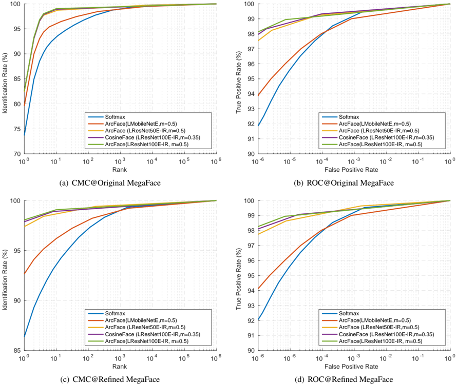In Table 9, we use the whole refined MS1M dataset to train models. We compare the performance of the proposed ArcFace with related baseline methods, e.g . Softmax, Triplet, SphereFace, and CosineFace. The proposed ArcFace obtains the best performance before and after the distractors refinement. After the overlapped face images are removed from the one million distractors, the identification performance significantly improves. We believe that the results on the manually refined MegaFace dataset are more reliable, and the performance of face identification under million distractors is better than we think [2]. To strictly follow the evaluation instructions on MegaFace, we need to remove all of the identities appearing in the FaceScrub dataset from our training data. We calculate the feature centre for each identity in the refined MS1M dataset and the FaceScrub dataset. We find that 578 identi- | Backbones | LFW ( % ) | CFP-FP ( % ) | AgeDB-30 ( % ) | Speed(ms) | Model-Size(MB) | |-----------------------------|-------------|----------------|------------------|-------------|------------------| | LResNet50E-IR | 99.75 | 96.58 | 93.53 | 8.9 | 167 | | SE-LResNet50E-IR | 99.78 | 96.82 | 93.83 | 13 | 169 | | LResNet100E-IR | 99.75 | 96.95 | 94.4 | 15.4 | 250 | | SE-LResNet100E-IR | 99.71 | 97.01 | 94.23 | 23.8 | 252 | | LResNet101(Bottle Neck)E-IR | 99.76 | 96.72 | 93.68 | 49.2 | 294 | | LMobileNetE | 99.63 | 95.81 | 91.85 | 4.2 | 112 | | LDenseNet161E | 99.71 | 96.51 | 93.68 | 29.3 | 315 | | LDPN92E | 99.71 | 96.82 | 94.18 | 38.1 | 393 | | LDPN107E | 99.76 | 96.94 | 94.9 | 58.8 | 581 | | LInception-ResNet-v2 | 99.75 | 97.15 | 95.35 | 53.6 | 642 | Table 8. Accuracy ( % ), speed (ms) and model size (MB) comparison between different backbones (Softmax@VGG2) | Methods | Rank1@ 10 6 | VR@FAR 10 - 6 | Rank1@ 10 6 (R) | VR@FAR 10 - 6 (R) | |-----------------------------------------|---------------|-----------------|-------------------|---------------------| | Softmax | 78.89 | 94.95 | 91.43 | 94.95 | | Softmax-pretrain,Triplet-finetune | 80.6 | 94.65 | 94.08 | 95.03 | | Softmax-pretrain@VGG2, Triplet-finetune | 78.87 | 95.43 | 93.96 | 95.07 | | SphereFace(m=4, λ =5) | 82.95 | 97.66 | 97.43 | 97.66 | | CosineFace(m=0.35) | 82.75 | 98.41 | 98.33 | 98.41 | | ArcFace(m=0.4) | 82.29 | 98.2 | 98.1 | 97.83 | | ArcFace(m=0.5) | 83.27 | 98.48 | 98.36 | 98.48 | Table 9. Identification and verification results of different methods on MegaFace Challenge1 (LResNet100E-IR@MS1M). 'Rank 1' refers to the rank-1 face identification accuracy and 'VR' refers to face verification TAR (True Accepted Rate) at 10 -6 FAR (False Accepted Rate). (R) denotes the refined version of MegaFace dataset. ties from the refined MS1M dataset have a close distance (cosine similarity is higher than 0 . 45 ) with the identities from the FaceScrub dataset. We remove these 578 identities from the refined MS1M dataset and compare the proposed ArcFace to other baseline methods in Table 10. ArcFace still outperforms CosineFace with a slight performance drop compared to Table 9. But for Softmax, the identification rate drops obviously from 78 . 89% to 73 . 66% after the suspectable overlap identities are removed from the training data. On the refined MegaFace testset, the verification result of CosineFace is slightly higher than that of ArcFace. This is because we read the verification results which are closest to FAR=1e-6 from the outputs of the devkit. As we can see from Figure 8, the proposed ArcFace always outperforms CosineFace under both identification and verification metric. ## 3.5. Further Improvement by Triplet Loss Due to the limitation of GPU memory, it is hard to train Softmax-based methods, e.g . SphereFace, CosineFace and ArcFace, with millions of identities. One practical solution is to employ metric learning methods, and the most widely used method is the Triplet loss [35, 22]. However, the converging speed of Triplet loss is relatively slow. To this end, we explore Triplet loss to fine-turn exist face recognition models which are trained with Softmax based methods. For Triplet loss fine-tuning, we use the LResNet100EIR network and set learning rate at 0 . 005 , momentum at 0 and weight decay at 5 e -4 . As shown in Table 11, we give the verification accuracy by Triplet loss fine-tuning on the AgeDB-30 dataset. We find that (1) The Softmax model trained on a dataset with fewer identity numbers ( e.g . VGG2 with 8,631 identities) can be obviously improved by Triplet loss fine-tuning on a dataset with more identity numbers ( e.g . MS1M with 85k identities). This improvement confirms the effectiveness of the two-step training strategy, and this strategy can significantly accelerate the whole model training compared to training Triplet loss from scratch. (2) The Softmax model can be further improved by Triplet loss fine-tuning on the same dataset, which proves that the local refinement can improve the global model. (3) The excellence of margin improved Softmax methods, e.g . SphereFace, CosineFace, and ArcFace, can be kept and further improved by Triplet loss fine-tuning, which also verifies that local metric learning method, e.g . Triplet loss, is complementary to global hypersphere metric learning based methods. As the margin used in Triplet loss is the Euclidean distance, we will investigate Triplet loss with the angular margin recently. Table 10. Identification and verification results of different methods on MegaFace Challenge1 (Methods@ MS1M - FaceScrub). 'Rank 1' refers to the rank-1 face identification accuracy and 'VR' refers to face verification TAR (True Accepted Rate) at 10 -6 FAR (False Accepted Rate). (R) denotes the refined version of MegaFace dataset. | Methods | Rank1@ 10 6 | VR@FAR 10 - 6 | Rank1@ 10 6 (R) | VR@FAR 10 - 6 (R) | |------------------------------|---------------|-----------------|-------------------|---------------------| | Softmax | 73.66 | 91.5 | 86.37 | 91.5 | | CosineFace(m=0.35) | 82.49 | 97.95 | 97.88 | 98.07 | | ArcFace(LMobileNetE,m=0.5) | 79.58 | 93 | 92.65 | 94 | | ArcFace(LResNet50E-IR,m=0.5) | 82.42 | 97.23 | 97.39 | 97.63 | | ArcFace(LResNet50E-IR,m=0.5) | 82.55 | 98.33 | 98.06 | 97.94 | Figure 8. (a) and (c) report CMC curves of different methods with 1M distractors on MegaFace Set 1. (b) and (d) give the ROC curves of different methods with 1M distractors on MegaFace Set 1. (a) and (b) are eveluated on the original MegaFace dataset, while (c) and (d) are evaluated on the refined MegaFace Dataset. <details> <summary>Image 11 Details</summary>  ### Visual Description ## Line Graphs: Comparative Performance of Face Recognition Models on CMC and ROC Metrics ### Overview The image contains four line graphs comparing the performance of face recognition models across two datasets (Original MegaFace and Refined MegaFace) using two evaluation metrics: CMC (Cumulative Match Characteristic) and ROC (Receiver Operating Characteristic). Each graph evaluates five models: Softmax, ArcFace with different backbones (LMobileNetE, LResNet50E-IR, LResNet100E-IR) and parameters (m=0.5 or m=0.35). The graphs are arranged in a 2x2 grid, with CMC metrics on the top row and ROC metrics on the bottom row. --- ### Components/Axes #### Graph (a): CMC@Original MegaFace - **X-axis**: Rank (logarithmic scale: 10⁰ to 10⁶) - **Y-axis**: Identification Rate (%) (linear scale: 70% to 100%) - **Legend**: Bottom-right corner, labels include: - Softmax (blue) - ArcFace(LMobileNetE, m=0.5) (orange) - ArcFace(LResNet50E-IR, m=0.5) (purple) - CosineFace(LResNet100E-IR, m=0.35) (green) - ArcFace(LResNet100E-IR, m=0.5) (red) #### Graph (b): ROC@Original MegaFace - **X-axis**: False Positive Rate (logarithmic scale: 10⁻⁶ to 10⁰) - **Y-axis**: True Positive Rate (%) (linear scale: 90% to 100%) - **Legend**: Bottom-right corner, same labels as (a). #### Graph (c): CMC@Refined MegaFace - **X-axis**: Rank (logarithmic scale: 10⁰ to 10⁶) - **Y-axis**: Identification Rate (%) (linear scale: 85% to 100%) - **Legend**: Bottom-right corner, same labels as (a). #### Graph (d): ROC@Refined MegaFace - **X-axis**: False Positive Rate (logarithmic scale: 10⁻⁶ to 10⁰) - **Y-axis**: True Positive Rate (%) (linear scale: 90% to 100%) - **Legend**: Bottom-right corner, same labels as (a). --- ### Detailed Analysis #### Graph (a): CMC@Original MegaFace - **Trends**: - All models show increasing Identification Rate with lower Rank. - **ArcFace(LResNet100E-IR, m=0.5)** (red) achieves the highest Identification Rate (~99% at Rank 10³). - **Softmax** (blue) lags significantly, reaching ~95% at Rank 10⁴. - **ArcFace(LMobileNetE, m=0.5)** (orange) and **CosineFace(LResNet100E-IR, m=0.35)** (green) perform similarly, with ~97% at Rank 10³. #### Graph (b): ROC@Original MegaFace - **Trends**: - All models achieve high True Positive Rates (>97%) at low False Positive Rates (<10⁻³). - **ArcFace(LResNet100E-IR, m=0.5)** (red) and **CosineFace(LResNet100E-IR, m=0.35)** (green) dominate, maintaining ~99% TPR at FPR <10⁻⁴. - **Softmax** (blue) underperforms, with TPR ~93% at FPR 10⁻². #### Graph (c): CMC@Refined MegaFace - **Trends**: - Similar to (a), but all models show slightly improved performance. - **ArcFace(LResNet100E-IR, m=0.5)** (red) reaches ~99.5% at Rank 10³. - **Softmax** (blue) improves marginally to ~96% at Rank 10⁴. #### Graph (d): ROC@Refined MegaFace - **Trends**: - All models achieve near-perfect TPR (>98%) at low FPR (<10⁻³). - **ArcFace(LResNet100E-IR, m=0.5)** (red) and **CosineFace(LResNet100E-IR, m=0.35)** (green) maintain ~99.5% TPR at FPR <10⁻⁴. - **Softmax** (blue) improves to ~94% at FPR 10⁻². --- ### Key Observations 1. **ArcFace superiority**: ArcFace variants consistently outperform Softmax across all metrics and datasets. 2. **Backbone impact**: LResNet100E-IR backbones (e.g., ArcFace and CosineFace) achieve the highest accuracy, suggesting deeper networks improve performance. 3. **Parameter sensitivity**: The `m` parameter in ArcFace (e.g., m=0.5 vs. m=0.35) has minimal impact on performance in this dataset. 4. **Refinement effect**: Refined MegaFace datasets show marginally better results than Original MegaFace, but differences are small (~1-2% improvement). --- ### Interpretation The data demonstrates that **ArcFace with LResNet100E-IR backbones** is the most effective model for face recognition, achieving near-perfect Identification Rates and True Positive Rates. Softmax, a traditional baseline, underperforms significantly, highlighting the advantages of modern deep learning approaches. The slight improvements in Refined MegaFace suggest dataset quality impacts model performance, but architectural choices (e.g., ArcFace) remain the dominant factor. The `m` parameter in ArcFace appears less critical in this context, indicating robustness across parameter settings. These results align with prior research emphasizing the importance of deep feature extraction in face recognition tasks. </details> ## 4. Conclusions In this paper, we contribute to improving deep face recognition from data refinement, network settings and loss function designs. We have (1) refined the largest public available training dataset (MS1M) and test dataset (MegaFace); (2) explored different network settings and analysed the trade-off between accuracy and speed; (3) proposed a geometrically interpretable loss function called ArcFace and explained why the proposed ArcFace is better than Softmax, SphereFace and CosineFace from the view of semi-hard sample distributions; (4) obtained state-of-theart performance on the MegaFace dataset in a totally repro- Table 11. Improve verification accuracy by Triplet loss fine-tuning (LResNet100E-IR). | Dataset@Loss | AgeDB-30 | |-------------------------------|------------| | VGG2@Softmax | 94.4 | | VGG2@Softmax, MS1M@Triplet | 97.5 | | MS1M@Softmax | 95.56 | | MS1M@Softmax, MS1M@Triplet | 97.16 | | MS1M@SphereFace | 97.56 | | MS1M@SphereFace, MS1M@Triplet | 97.85 | | MS1M@CosineFace | 97.91 | | MS1M@CosineFace, MS1M@Triplet | 97.98 | | MS1M@ArcFace | 98.08 | | MS1M@ArcFace, MS1M@Triplet | 98.15 | ducible way. ## References - [1] Fg-net aging database, www-prima.inrialpes.fr/fgnet/.2002. 6 - [2] http://megaface.cs.washington.edu/results/facescrub.html. 1, 2, 9 - [3] https://github.com/davidsandberg/facenet. 2 - [4] https://www.nist.gov/programs-projects/face-recognitionvendor-test-frvt-ongoing. 1 - [5] http://www.yitutech.com/intro/. 1 - [6] A. Bansal, A. Nanduri, C. D. Castillo, R. Ranjan, and R. Chellappa. Umdfaces: An annotated face dataset for training deep networks. arXiv:1611.01484v2 , 2016. 1 - [7] Q. Cao, L. Shen, W. Xie, O. M. Parkhi, and A. Zisserman. Vggface2: A dataset for recognising faces across pose and age. arXiv:1710.08092 , 2017. 1, 2, 3, 6 - [8] T. Chen, M. Li, Y. Li, M. Lin, N. Wang, M. Wang, T. Xiao, B. Xu, C. Zhang, and Z. Zhang. Mxnet: A flexible and efficient machine learning library for heterogeneous distributed systems. arXiv:1512.01274 , 2015. 7 - [9] Y. Chen, J. Li, H. Xiao, X. Jin, S. Yan, and J. Feng. Dual path networks. In Advances in Neural Information Processing Systems , pages 4470-4478, 2017. 8 - [10] J. Deng, Y. Zhou, and S. Zafeiriou. Marginal loss for deep face recognition. In CVPRW , 2017. 2, 6 - [11] Y. Guo, L. Zhang, Y. Hu, X. He, and J. Gao. Ms-celeb-1m: Adataset and benchmark for large-scale face recognition. In European Conference on Computer Vision , pages 87-102. Springer, 2016. 1, 2, 6 - [12] D. Han, J. Kim, and J. Kim. Deep pyramidal residual networks. arXiv:1610.02915 , 2016. 8 - [13] K. He, X. Zhang, S. Ren, and J. Sun. Delving deep into rectifiers: Surpassing human-level performance on imagenet classification. In Proceedings of the IEEE international conference on computer vision , pages 1026-1034, 2015. 8 - [14] K. He, X. Zhang, S. Ren, and J. Sun. Deep residual learning for image recognition. In Proceedings of the IEEE Conference on Computer Vision and Pattern Recognition , pages 770-778, 2016. 2, 8 - [15] K. He, X. Zhang, S. Ren, and J. Sun. Identity mappings in deep residual networks. In European Conference on Computer Vision , pages 630-645. Springer, 2016. 2 - [16] A. G. Howard, M. Zhu, B. Chen, D. Kalenichenko, W. Wang, T. Weyand, M. Andreetto, and H. Adam. Mobilenets: Efficient convolutional neural networks for mobile vision applications. arXiv:1704.04861 , 2017. 2, 8 - [17] J. Hu, L. Shen, and G. Sun. Squeeze-and-excitation networks. arXiv:1709.01507 , 2017. 8 - [18] G. Huang, Z. Liu, K. Q. Weinberger, and L. van der Maaten. Densely connected convolutional networks. CVPR , 2016. 8 - [19] G. B. Huang, M. Ramesh, T. Berg, and E. Learned-Miller. Labeled faces in the wild: A database for studying face recognition in unconstrained environments. Technical report, Technical Report 07-49, University of Massachusetts, Amherst, 2007. 5, 6 - [20] S. Ioffe and C. Szegedy. Batch normalization: Accelerating deep network training by reducing internal covariate shift. In International Conference on Machine Learning , pages 448456, 2015. 8 - [21] I. Kemelmacher-Shlizerman, S. M. Seitz, D. Miller, and E. Brossard. The megaface benchmark: 1 million faces for recognition at scale. In Proceedings of the IEEE Conference on Computer Vision and Pattern Recognition , pages 48734882, 2016. 1, 2, 5, 6 - [22] J. Liu, Y . Deng, T. Bai, Z. Wei, and C. Huang. Targeting ultimate accuracy: Face recognition via deep embedding. arXiv preprint arXiv:1506.07310 , 2015. 10 - [23] W. Liu, Y. Wen, Z. Yu, M. Li, B. Raj, and L. Song. Sphereface: Deep hypersphere embedding for face recognition. CVPR , 2017. 1, 2, 3, 4, 7, 9 - [24] W. Liu, Y. Wen, Z. Yu, and M. Yang. Large-margin softmax loss for convolutional neural networks. In ICML , pages 507516, 2016. 2, 3 - [25] W. Liu, Y.-M. Zhang, X. Li, Z. Yu, B. Dai, T. Zhao, and L. Song. Deep hyperspherical learning. In Advances in Neural Information Processing Systems , pages 3953-3963, 2017. 3 - [26] Y. Liu, H. Li, and X. Wang. Rethinking feature discrimination and polymerization for large-scale recognition. arXiv:1710.00870 , 2017. 3 - [27] S. Moschoglou, A. Papaioannou, C. Sagonas, J. Deng, I. Kotsia, and S. Zafeiriou. Agedb: The first manually collected in-the-wild age database. In Proceedings of the IEEE Conference on Computer Vision and Pattern Recognition Workshop , 2017. 5, 6 - [28] H.-W. Ng and S. Winkler. A data-driven approach to cleaning large face datasets. In Image Processing (ICIP), 2014 IEEE International Conference on , pages 343-347. IEEE, 2014. 6 - [29] H. V. Nguyen and L. Bai. Cosine similarity metric learning for face verification. In ACCV , pages 709-720, 2010. 3 - [30] C. J. Parde, C. Castillo, M. Q. Hill, Y . I. Colon, S. Sankaranarayanan, J.-C. Chen, and A. J. O'Toole. Deep convolutional neural network features and the original image. arXiv:1611.01751 , 2016. 3 - [31] O. M. Parkhi, A. Vedaldi, and A. Zisserman. Deep face recognition. In BMVC , volume 1, page 6, 2015. 1, 2, 3 - [32] G. Pereyra, G. Tucker, J. Chorowski, Ł. Kaiser, and G. Hinton. Regularizing neural networks by penalizing confident output distributions. arXiv:1701.06548 , 2017. 3 - [33] R. Ranjan, C. D. Castillo, and R. Chellappa. L2constrained softmax loss for discriminative face verification. arXiv:1703.09507 , 2017. 3 - [34] O. Russakovsky, J. Deng, H. Su, J. Krause, S. Satheesh, S. Ma, Z. Huang, A. Karpathy, A. Khosla, M. Bernstein, et al. Imagenet large scale visual recognition challenge. International Journal of Computer Vision , 115(3):211-252, 2015. 7 - [35] F. Schroff, D. Kalenichenko, and J. Philbin. Facenet: A unified embedding for face recognition and clustering. In CVPR , 2015. 1, 2, 5, 10 - [36] S. Sengupta, J.-C. Chen, C. Castillo, V. M. Patel, R. Chellappa, and D. W. Jacobs. Frontal to profile face verification in the wild. In WACV , pages 1-9, 2016. 5, 6 - [37] K. Simonyan and A. Zisserman. Very deep convolutional networks for large-scale image recognition. arXiv preprint arXiv:1409.1556 , 2014. 2 - [38] N. Srivastava, G. E. Hinton, A. Krizhevsky, I. Sutskever, and R. Salakhutdinov. Dropout: a simple way to prevent neural networks from overfitting. Journal of machine learning research , 15(1):1929-1958, 2014. 8 - [39] Y. Sun, Y. Chen, X. Wang, and X. Tang. Deep learning face representation by joint identification-verification. In Advances in neural information processing systems , pages 1988-1996, 2014. 2 - [40] C. Szegedy, S. Ioffe, V. Vanhoucke, and A. A. Alemi. Inception-v4, inception-resnet and the impact of residual connections on learning. In AAAI , pages 4278-4284, 2017. 2, 8 - [41] C. Szegedy, W. Liu, Y. Jia, P. Sermanet, S. Reed, D. Anguelov, D. Erhan, V. Vanhoucke, and A. Rabinovich. Going deeper with convolutions. In Proceedings of the IEEE Conference on Computer Vision and Pattern Recognition , pages 1-9, 2015. 2 - [42] Y. Taigman, M. Yang, M. Ranzato, and L. Wolf. Deepface: Closing the gap to human-level performance in face verification. In CVPR , 2014. 1, 2 - [43] TencentAILab. Facecnn v1. 9/21/2017. 1, 2, 3, 4, 9 - [44] F. Wang, W. Liu, H. Liu, and J. Cheng. Additive margin softmax for face verification. In arXiv:1801.05599 , 2018. 1, 2, 3, 4, 9 - [45] F. Wang, X. Xiang, J. Cheng, and A. L. Yuille. Normface: l 2 hypersphere embedding for face verification. arXiv:1704.06369 , 2017. 3 - [46] Y. Wen, K. Zhang, Z. Li, and Y. Qiao. A discriminative feature learning approach for deep face recognition. In European Conference on Computer Vision , pages 499-515. Springer, 2016. 2, 3, 7 - [47] X. Wu, R. He, Z. Sun, and T. Tan. A light cnn for deep face representation with noisy labels. arXiv preprint arXiv:1511.02683 , 2015. 1 - [48] D. Yi, Z. Lei, S. Liao, and S. Z. Li. Learning face representation from scratch. arXiv preprint arXiv:1411.7923 , 2014. 1 - [49] K. Zhang, Z. Zhang, Z. Li, and Y. Qiao. Joint face detection and alignment using multitask cascaded convolutional networks. IEEE Signal Processing Letters , 23(10):1499-1503, 2016. 7 - [50] X. Zhang, Z. Fang, Y. Wen, Z. Li, and Y. Qiao. Range loss for deep face recognition with long-tail. ICCV , 2017. 1, 2, 3 - [51] X. Zhang, X. Zhou, M. Lin, and J. Sun. Shufflenet: An extremely efficient convolutional neural network for mobile devices. arXiv:1707.01083 , 2017. 2