1802.04712

# ArXiv Paper 1802.04712v1 ## Attention-based Deep Multiple Instance Learning Maximilian Ilse * 1 Jakub M. Tomczak * 1 Max Welling 1 ## Abstract Multiple instance learning (MIL) is a variation of supervised learning where a single class label is assigned to a bag of instances. In this paper, we state the MIL problem as learning the Bernoulli distribution of the bag label where the bag label probability is fully parameterized by neural networks. Furthermore, we propose a neural network-based permutation-invariant aggregation operator that corresponds to the attention mechanism. Notably, an application of the proposed attention-based operator provides insight into the contribution of each instance to the bag label. We show empirically that our approach achieves comparable performance to the best MIL methods on benchmark MIL datasets and it outperforms other methods on a MNIST-based MIL dataset and two real-life histopathology datasets without sacrificing interpretability. ## 1. Introduction In typical machine learning problems like image classification it is assumed that an image clearly represents a category (a class). However, in many real-life applications multiple instances are observed and only a general statement of the category is given. This scenario is called multiple instance learning (MIL) (Dietterich et al., 1997; Maron & Lozano-P´ erez, 1998) or, learning from weakly annotated data (Oquab et al., 2014). The problem of weakly annotated data is especially apparent in medical imaging (Quellec et al., 2017) ( e.g. , computational pathology, mammography or CT lung screening) where an image is typically described by a single label (benign/malignant) or a Region of Interest (ROI) is roughly given. MIL deals with a bag of instances for which a single class label is assigned. Hence, the main goal of MIL is to learn a model that predicts a bag label, e.g. , a medical diagnosis. An additional challenge is to discover which instances in the * Equal contribution 1 University of Amsterdam, the Netherlands. Correspondence to: Maximilian Ilse < M.Ilse@uva.nl > , Jakub M. Tomczak < J.M.Tomczak@uva.nl > . bag influences the bag label. In other words, it is possible to interpret instances as ROIs. In the medical domain the former task is of great interest because of legal issues 1 and its use in clinical practice. In order to solve the primary task of a bag classification different methods are proposed, such as utilizing similarities among bags (Cheplygina et al., 2015b), embedding instances to a compact low-dimensional representation that is further fed to a bag-level classifier (Andrews et al., 2003; Chen et al., 2006), and combining responses of an instance-level classifier (Ramon & De Raedt, 2000; Raykar et al., 2008; Zhang et al., 2006). Only the last approach is capable of providing interpretable results. However, it was shown that the instance level accuracy of such methods is low (Kandemir & Hamprecht, 2015) and in general there is a huge disagreement among MIL methods at the instance level (Cheplygina et al., 2015a). These issues call into question the usability of current MIL models for interpreting the final decision. In this paper, we propose a new method that aims at incorporating interpretability to the MIL approach and increasing its flexibility. We formulate the MIL model using the Bernoulli distribution for the bag label and train it by optimizing the (penalized) log-likelihood function. We show that the application of the Fundamental Theorem of Symmetric Functions provides a general procedure for modeling the bag label probability (the bag score function) that consists of three steps: (i) a transformation of instances to a low-dimensional embedding, (ii) a permutation-invariant (symmetric) aggregation function, and (iii) a final transformation to the bag probability. We propose to parameterize all transformations using neural networks ( i.e. , a combination of convolutional and fully-connected layers), which increases the flexibility of the approach and allows to train the model in an end-to-end manner by optimizing an unconstrained objective function. Last but not least, we propose to replace widely-used permutation-invariant operators such as the maximum operator ( max ) and the mean operator ( mean ) by a trainable weighted average where weights are given by a two-layered neural network. The two-layered neural network corresponds to the attention mechanism (Bahdanau et al., 2014; Raffel & Ellis, 2015). Notably, the attention 1 According to the European Union General Data Protection Regulation (taking effect 2018), a user should have the right to obtain an explanation of the decision reached. weights allow us to interpret how instances contribute to the final decision, which could be further used to highlight possible ROIs. In the experiments we show that our model is on a par with the best classical MIL methods on common benchmark MIL datasets, and that it outperforms other methods on a MNIST-based MIL problem as well as two real-life histology image datasets. Moreover, in the image datasets we provide empirical evidence that our model can indicate the majority of the positive instances contributing to the bag label. ## 2. Methodology ## 2.1. Multiple instance learning (MIL) Problem formulation In the classical (binary) supervised learning problem one aims at finding a model that predicts a value of a target variable, y ∈ { 0 , 1 } , for a given instance, x ∈ R D . In the case of the MIL problem, however, instead of a single instance there is a bag of instances, X = { x 1 , . . . , x K } , that exhibit neither dependency nor ordering among each other. We assume that K could vary for different bags. There is also a single binary label Y associated with the bag. Furthermore, we assume that individual labels exist for the instances within a bag, i.e. , y 1 , . . . , y K and y k ∈ { 0 , 1 } , for k = 1 , . . . , K , however, there is no access to those labels and they remain unknown during training. We can re-write the assumptions of the MIL problem in the following form: $$y = \begin{cases} 0 , & if \sum _ { k = 1 } ^ { n } y _ { k } = 0 , \\ 1 , & otherwise . \end{cases}$$ These assumptions imply that a MIL model must be permutation-invariant . Further, the two statements could be re-formulated in a compact form using the maximum operator: $$y = \frac { 1 } { x } ( x > 0 )$$ Learning a model that tries to optimize an objective based on the maximum over instance labels would be problematic at least for two reasons. First, all gradient-based learning methods would encounter issues with vanishing gradients. Second, this formulation is suitable only for the approach with the instance-level classifier. In order to make the learning problem easier, we propose to train a MIL model by optimizing the (penalized) loglikelihood function where the bag label is distributed according to the Bernoulli distribution with the parameter θ ( X ) ∈ [0 , 1] , i.e. , the probability of Y = 1 given the bag of instances X . A penalty term in the objective function could correspond to a widely-used regularizer like weight decay. MIL approaches In the MIL setting the bag probability θ ( X ) must be permutation-invariant since we assume neither ordering nor dependency of instances within a bag. Therefore, the MIL problem can be considered in terms of a specific form of the Fundamental Theorem of Symmetric Functions with monomials given by the following theorem (Zaheer et al., 2017): Theorem 1. A scoring function for a set of instances X , S ( X ) ∈ R , is a symmetric function (i.e., permutationinvariant to the elements in X ) , if and only if it can be decomposed in the following form: $$S ( X ) = g ( \sum f ( x ) ,$$ where f and g are suitable transformations. This theorem provides a general strategy for modeling the bag probability using the decomposition given in (3). A similar decomposition with max instead of sum is given by the following theorem (Qi et al., 2017): Theorem 2. For any ε > 0 , a Hausdorff continuous symmetric function S ( X ) ∈ R can be arbitrarily approximated by a function in the form g ( max x ∈ X f ( x ) ) , where max is the element-wise vector maximum operator and f and g are continuous functions, that is: $$\vert S ( X ) - g ( \max _ { x \in X } f ( x ) ) \vert < ε .$$ The difference between Theorems 1 and 2 is that the former is a universal decomposition while the latter provides an arbitrary approximation. Nonetheless, they both formulate a general three-step approach for classifying a bag of instances: (i) a transformation of instances using the function f , (ii) a combination of transformed instances using a symmetric (permutation-invariant) function σ , (iii) a transformation of combined instances transformed by f using a function g . Finally, the expressiveness of the score function relies on the choice of classes of functions for f and g . In the MIL problem formulation the score function in both theorems is the probability θ ( X ) and the permutationinvariant function σ is referred to as the MIL pooling. The choice of functions f , g and σ determines a specific approach to modeling the label probability. For a given MIL operator there are two main MIL approaches: - (i) The instance-level approach : The transformation f is an instance-level classifier that returns scores for each instance. Then individual scores are aggregated by MIL pooling to obtain θ ( X ) . The function g is the identity function. - (ii) The embedding-level approach : The function f maps instances to a low-dimensional embedding. MIL pooling is used to obtain a bag representation that is independent of the number of instances in the bag. The bag representation is further processed by a bag-level classifier to provide θ ( X ) . It is advocated in Wang et al. (2018) that the latter approach is preferable to the former one in terms of the bag level classification performance. Since the individual labels are unknown, there is a threat that the instance-level classifier might be trained insufficiently and it introduces additional error to the final prediction. The embedding-level approach determines a joint representation of a bag and therefore it does not introduce additional bias to the bag-level classifier. On the other hand, the biggest disadvantage of the embedding-level approach is limited interpretability of a result while the instance-level approach provides a label (or a score) per instance that straightforwardly indicates which instance is positive or negative. We will show how to modify the embedding-level approach to be interpretable by using a new MIL pooling. ## 2.2. MIL with Neural Networks In classical MIL problems it is assumed that instances are represented by features that do not require further processing, i.e. , f is the identity. However, for some tasks like image or text analysis additional steps of feature extraction are necessary. Additionally, Theorem 1 and 2 indicate that for a flexible enough class of functions we can model any permutation-invariant score function. Therefore, we consider a class of transformations that are parameterized by neural networks with parameters ψ , f ψ ( · ) , that transform the k -th instance into a low-dimensional embedding, h k = f ψ ( x k ) , where h k ∈ H such that H = [0 , 1] for the instance-based approach and H = R M for the embeddingbased approach. 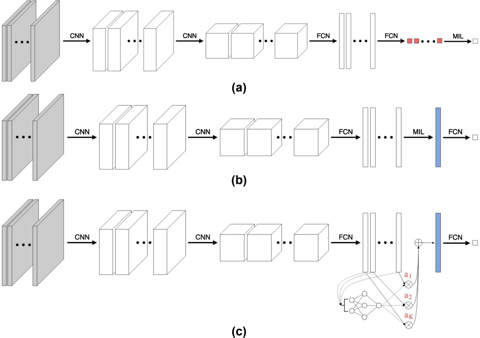Eventually, the parameter θ ( X ) is determined by a transformation g φ : H K → [0 , 1] . In the instance-based approach the transformation g φ is simply the identity, while in the embedding-based approach it could be also parameterized by a neural network with parameters φ . The former approach is depicted in Figure 6(a) and the latter in Figure 6(b) in the Appendix. The idea of parameterizing all transformations using neural networks is very appealing because the whole approach can be arbitrarily flexible and it can be trained end-to-end by backpropagation. The only restriction is that the MIL pooling must be differentiable. ## 2.3. MIL pooling The formulation of the MIL problem requires the MIL pooling σ to be permutation-invariant. As shown in Theorem 1 and 2, there are two MIL pooling operators that ensure the score function ( i.e. , the bag probability) to be a symmetric function, namely, the maximum operator: $$\forall m = 1 , \ldots , M : z _ { m } = k = 1$$ and the mean operator: 2 $$z = - \sum _ { k = 1 } ^ { K } h _ { k }$$ In fact, other operators could be used that are closely related to max( · ) , such as, the convex maximum operator ( i.e. , log-sum-exp) (Ramon & De Raedt, 2000), Integrated Segmentation and Recognition (Keeler et al., 1991), noisyor (Maron & Lozano-P´ erez, 1998) and noisy-and (Kraus et al., 2016). These MIL pooling operators could replace max in Theorem 2 and proofs would follow in a similar manner (see Supplementary in Qi et al. (2017) for a detailed proof for the maximum operator). All of these operators are differentiable, hence, they could be easily used as a MIL pooling layer in a deep neural network architecture. ## 2.4. Attention-based MIL pooling All MIL pooling operators mentioned in the previous section have a clear disadvantage, namely, they are pre-defined and non-trainable. For instance, the max -operator could be a good choice in the instance-based approach but it might be inappropriate for the embedding-based approach. Similarly, the mean operator is definitely a bad MIL pooling to aggregate instance scores, although, it could succeed in calculating the bag representation. Therefore, a flexible and adaptive MIL pooling could potentially achieve better results by adjusting to a task and data. Ideally, such MIL pooling should also be interpretable, a trait that is missing in all operators mentioned in Section 2.3. Attention mechanism We propose to use a weighted average of instances (low-dimensional embeddings) where weights are determined by a neural network. Additionally, the weights must sum to 1 to be invariant to the size of a bag. The weighted average fulfills the requirements of the Theorem 1 where the weights together with the embeddings are part of the f function. Let H = { h 1 , . . . , h K } be a bag of K embeddings, then we propose the following MIL pooling: $$z = \sum _ { k = 1 } ^ { K } a _ { k } b _ { k } ,$$ where: $$h ( V h _ { k } ^ { T } ) , \quad ( 8 )$$ where w ∈ R L and V ∈ R L × M are parameters. We use the softmax non-linearity to ensure that the attention weights 2 Notice that the weight 1 K can be seen as a part of the f function. will sum to 1 . Moreover, we utilize the hyperbolic tangent ( tanh( · ) ) element-wise non-linearity to include both negative and positive values for proper gradient flow. The proposed construction allows to discover (dis)similarities among instances. Alternative expressions include the dot product among instances or more layers within the proposed MIL pooling. However, our preliminary experiments showed that the alternative formulations result in either under- or overfitting, respectively. Interestingly, the proposed MIL pooling corresponds to a version of the attention mechanism (Lin et al., 2017; Raffel &Ellis, 2015). The main difference is that typically in the attention mechanism all instances are sequentially dependent while here we assume that all instances are independent. Therefore, a naturally arising question is whether the attention mechanism could work without sequential dependencies among instances, and if it will not learn the mean operator. We will address this issue in the experiments. Gated attention mechanism Furthermore, we notice that the tanh( · ) non-linearity could be inefficient to learn complex relations. Our concern follows from the fact that tanh(x) is approximately linear for x ∈ [ -1 , 1 ], which could limit the final expressiveness of learned relations among instances. Therefore, we propose to additionally use the gating mechanism (Dauphin et al., 2016) together with tanh( · ) non-linearity that yields: $$\alpha _ { k } = \softmax ( w ^ { T } ( tanh ( )$$ where U ∈ R L × M are parameters, is an element-wise multiplication and sigm( · ) is the sigmoid element-wise nonlinearity. The gating mechanism introduces a learnable nonlinearity that potentially removes the troublesome linearity in tanh( · ) . Flexibility In principle, the proposed attention-based MIL pooling allows to assign different weights to instances within a bag and hence the final representation of the bag could be highly informative for the bag-level classifier. In other words, it should pick such instances that are crucial for the final classification. Moreover, application of the attention-based MIL pooling together with the transformations f and g parameterized by neural networks makes the whole model fully differentiable and adaptive. These two facts make the proposed MIL pooling a potentially very flexible operator that could model an arbitrary permutationinvariant score function. The proposed attention mechanism together with a deep MIL model is depicted in Figure 6(c) in the Appendix. Interpretability Ideally, in the case of a positive label ( Y = 1 ), high attention weights should be assigned to instances that are likely to have label y k = 1 . Namely, the attention mechanism allows to easily interpret the pro- vided decision in terms of instance-level labels. In fact, the attention network does not provide scores as the instancebased classifier does but it can be considered as a proxy to that. Therefore, the attention-based MIL pooling bridges the instance-level approach and the embedding-level approach. One needs to be aware that no information about the instance labels is provided. Therefore, for a positive bag the attention mechanism might assign relatively high weights to instances with y k = 0 , as they can still be helpful for the final classification. Nevertheless, from the practical point of view, e.g. , in the computational pathology, it is more desirable to provide ROIs together with the final diagnosis to a doctor. Therefore, the attention mechanism is potentially of great interest in practical applications. ## 3. Related work MIL pooling Typically, MIL approaches utilize either the mean pooling or the max pooling, while the latter is mostly used (Feng & Zhou, 2017; Pinheiro & Collobert, 2015; Zhu et al., 2017). Both operators are non-trainable which potentially limits their applicability. There are MIL pooling operators that contain global adaptive parameters, such as Noisy-AND (Kraus et al., 2016), however, their flexibility is restricted. We propose a fully trainable MIL pooling that adapts to new instances. MIL with neural networks In the classical work on MIL it is assumed that instances are represented by precomputed features and there is very little need to apply additional feature extraction. Nevertheless, recent work on utilizing fully-connected neural networks in MIL shows that it could still be beneficial (Wang et al., 2018). Similarly, in computer vision the idea of MIL combined with deep learning significantly improves final accuracy (Oquab et al., 2014). In this paper, we follow this line of research since it allows to apply a flexible class of transformations that can be trained end-to-end by backpropagation. MIL and attention The attention mechanism is widely used in deep learning for image captioning (Xu et al., 2015) or text analysis (Bahdanau et al., 2014; Lin et al., 2017). In the context of the MIL problem it has rarely been used and only in a very limited form. In Pappas & Popescu-Belis (2017) an attention-based MIL was proposed but attention weights were trained as parameters of an auxiliary linear regression model. The attention-based MIL operator was used very recently in Qi et al. (2017), however, the attention was calculated using the dot product and it performed worse than the max operator. Here, we propose to use a two-layered neural network to learn the MIL operator and we show that it outperforms commonly used MIL pooling operators. MIL for medical imaging The MIL seems to perfectly fit medical imaging where processing a whole image consisting of billions of pixels is computationally infeasible. Moreover, in the medical domain it is very difficult to obtain pixel-level annotations that drastically reduces number of available data. Therefore, it is tempting to divide a medical image into smaller patches that could be further considered as a bag with a single label (Quellec et al., 2017). This idea attracts a great interest in the computational histopathology where patches could correspond to cells that are believed to indicate malignant changes (Sirinukunwattana et al., 2016). Different MIL approaches were used for histopathology data, such as, Gaussian processes (Kandemir et al., 2014; 2016) or a two-stage approach with neural networks and EM algorithm to determine instance classes (Hou et al., 2016). Other applications of MIL methods in medical imaging are mammography (nodule) classification (Zhu et al., 2017), microscopy cell detection (Kraus et al., 2016), among others. In this paper, we show that the proposed attention-based deep MIL approach can be used not only to provide the final diagnosis but also to indicate ROIs in a histopathology slide that are extremely important in clinical practice. ## 4. Experiments In the experiments we aim at evaluating the proposed approach: a MIL model parameterized with neural networks and a (gated) attention-based pooling layer (ATTENTION and GATED-ATTENTION). We evaluate our approach on a number of different MIL datasets: five MIL benchmark datasets (MUSK1, MUSK2, FOX, TIGER, ELEPHANT), an MNIST-based image dataset (MNIST-BAGS) and two reallife histopathology datasets (BREAST CANCER, COLON CANCER). We want to verify two research questions in the experiments: (i) whether our approach achieves the best performance or is comparable to the best performing method, (ii) if our method can provide interpretable results by using the attention weights that indicate positive instances or ROIs. In order to obtain a fair comparison we use a common evaluation methodology, i.e. , 10-fold-cross-validation, and five repetitions per experiment. In the case of MNIST-BAGS we use a fixed division into training and test set. For all experiments we use modified versions of models that have shown high classification performance on the individual datasets (Wang et al., 2018; LeCun et al., 1998; Sirinukunwattana et al., 2016). The MIL pooling layers are either located before the last layer of the model (the embedded-based approach) or after last layer of the model (the instance-based approach). If an attention-based MIL pooling layer is used the number of parameters in V was determined using a validation set. We tested the following dimensions ( L ): 64, 128 and 256. The different dimensions only resulted in minor changes of the model's performance. For layers using the gated attention mechanism V and U have the same number of parameters. Finally, all layers were initialized according to Glorot & Bengio (2010) and biases were set to zero. We compare our approach to various MIL methods on the MIL benchmark datasets. On the image datasets our method is compared with instance-level and embedding-level neural networks and commonly used MIL pooling layers ( max and mean ). On MNIST-BAGS we include a SVM-based MIL model, called (MI-SVM). We do not present results of MI-SVM on the histopathology datasets since we could not train (including hyperparameter search and five times 10-fold-cross-validation procedure) the model in a reasonable amount of time. 3 In order to compare the bag level performance we use the following metrics: the classification accuracy (ACCURACY), precision (PRECISION), recall (RECALL), F-score (FSCORE), and the area under the receiver operating characteristic curve AUC. ## 4.1. Classical MIL datasets Details In the first experiment we aim at verifying whether our approach can compete with the best MIL methods on historically important benchmark datasets. Since all five datasets contain precomputed features and only a small number of instances and bags, neural networks are most likely not well suited. First we predict drug activity (MUSK1 and MUSK2). A molecule has the desired drug effect if and only if one or more of its conformations bind to the target binding site. Since molecules can adopt multiple shapes, a bag is made up of shapes belonging to the same molecule (Dietterich et al., 1997). The three remaining datasets, ELEPHANT, FOX and TIGER, contain features extracted from images. Each bag consists of a set of segments of an image. For each category, positive bags are images that contain the animal of interest, and negative bags are images that contain other animals (Andrews et al., 2003). For detailed information on the number of bags, instances and features in each dataset see Section 6.2 in the Appendix. In our experiments we use the same architecture as in the MI-Net model (Wang et al., 2018). To train the model we use SGD with the same hyperparameters as in Wang et al. (2018), see Table 7 in the Appendix. It is important to notice that only methods with prefix 'mi' in the Table 1 are interpretable since these use an instance classifier. Results and discussion The results of the experiment are presented in Table 1. Our approaches (ATTENTION and GATED-ATTENTION) are comparable with the best performing classical MIL methods (notice the standard error of the mean). This shows that the application of fully learnable architectures and the MIL operator is highly convenient since 3 Learning a single MI-SVM took approximately one week due to the large number of patches. Table 1. Results on classical MIL datasets. Experiments were run 5 times and an average of the classification accuracy ( ± a standard error of a mean) is reported. [1] (Andrews et al., 2003), [2] (G¨ artner et al., 2002), [3] (Zhang & Goldman, 2002) [4] (Zhou et al., 2009) [5] (Wei et al., 2017) [6] (Wang et al., 2018) | METHOD | MUSK1 | MUSK2 | FOX | TIGER | ELEPHANT | |------------------------------------------------------------------------------------------------------|---------------------------------------------------------------------------------------------------------------------------|---------------------------------------------------------------------------------------------------------------------------|---------------------------------------------------------------------------------------------------------------------------|---------------------------------------------------------------------------------------------------------------------------|---------------------------------------------------------------------------------------------------------------------------| | mi-SVM [1] MI-SVM [1] MI-Kernel [2] EM-DD [3] mi-Graph [4] miVLAD [5] miFV [5] mi-net [6] MI-NET [6] | 0.874 ± N/A 0.779 ± N/A 0.880 ± 0.031 0.849 ± 0.044 0.889 ± 0.033 0.871 ± 0.043 0.909 ± 0.040 0.889 ± 0.039 0.887 ± 0.041 | 0.836 ± N/A 0.843 ± N/A 0.893 ± 0.015 0.869 ± 0.048 0.903 ± 0.039 0.872 ± 0.042 0.884 ± 0.042 0.858 ± 0.049 0.859 ± 0.046 | 0.582 ± N/A 0.578 ± N/A 0.603 ± 0.028 0.609 ± 0.045 0.620 ± 0.044 0.620 ± 0.044 0.621 ± 0.049 0.613 ± 0.035 0.622 ± 0.038 | 0.784 ± N/A 0.840 ± N/A 0.842 ± 0.010 0.730 ± 0.043 0.860 ± 0.037 0.811 ± 0.039 0.813 ± 0.037 0.824 ± 0.034 0.830 ± 0.032 | 0.822 ± N/A 0.843 ± N/A 0.843 ± 0.016 0.771 ± 0.043 0.869 ± 0.035 0.850 ± 0.036 0.852 ± 0.036 0.858 ± 0.037 0.862 ± 0.034 | all elements of the architecture are trained by backpropagation, which can easily be parallelized on a GPU. ## 4.2. MNIST-bags Details The main disadvantage of the classical MIL benchmark datasets is that instances are represented by precomputed features. In order to consider a more challenging scenario, we propose to investigate a dataset that is created using the well-known MNIST image dataset. A bag is made up of a random number of 28 × 28 grayscale images taken from the MNIST dataset. The number of images in a bag is Gaussian-distributed and the closest integer value is taken. A bag is given a positive label if it contains one or more images with the label '9'. We chose '9' since it can be easily mistaken with '7' or '4'. We investigate the influence of the number of bags in the training set as well as the average number of instances per bag on the prediction performance. During evaluation we use a fixed number of 1000 test bags. For all experiments a LeNet5 model is used (LeCun et al., 1998), see Table 8 and 9 in the Appendix. The models are trained with the Adam optimization algorithm (Kingma & Ba, 2014). We keep the default parameters for β 1 and β 2 , see Table 10 in the Appendix. In addition, we compare our method with a SVM-based MIL method (MI-SVM) (Andrews et al., 2003) that uses a Gaussian kernel on raw pixel features 4 . In the experiments we use different numbers of the mean bag size, namely, 10 , 50 and 100 , and the variance 2 , 10 , 20 , respectively. Moreover, we use varying numbers of training bags, i.e. , 50 , 100 , 150 , 200 , 300 , 400 , 500 . These different settings allow us to verify how different number of training bags and different number of instances influence MIL models. We compare instance-based and embedding-based approaches parameterized with a neural network (LeNet5) 4 We use code provided with Doran & Ray (2014): //github.com/garydoranjr/misvm https: with mean and max MIL pooling. We use AUC as the evaluation metric. <details> <summary>Image 1 Details</summary>  ### Visual Description ## Line Chart: AUC Performance vs. Number of Training Bags ### Overview The chart compares the performance of five machine learning methods (MI-SVM, instance+MAX, embedding+MAX, Attention, Gated-Attention) in terms of Area Under the Curve (AUC) as the number of training bags increases from 100 to 500. All methods show improvement with more training data, with Gated-Attention and embedding+MAX achieving the highest AUC values. ### Components/Axes - **X-axis**: "Number of training bags" (100 to 500, increments of 100). - **Y-axis**: "AUC" (0.55 to 1.00, increments of 0.05). - **Legend**: Located in the bottom-right corner, mapping colors and line styles to methods: - **Blue dashed line with stars**: MI-SVM - **Orange dashed line with triangles**: instance+MAX - **Green dashed line with diamonds**: embedding+MAX - **Red dashed line with circles**: Attention - **Purple dashed line with squares**: Gated-Attention - **Error bars**: Vertical lines indicating variability in AUC measurements. ### Detailed Analysis 1. **MI-SVM (Blue)**: - Starts at ~0.70 AUC at 100 bags, rising steadily to ~0.95 at 500 bags. - Error bars are moderate, with the largest uncertainty at 100 bags (±0.05). 2. **instance+MAX (Orange)**: - Sharp initial increase from ~0.60 to ~0.95 between 100 and 200 bags. - Plateaus at ~0.95 for 300–500 bags. - High variability at 100 bags (±0.05), decreasing to ±0.02 at 500 bags. 3. **embedding+MAX (Green)**: - Gradual rise from ~0.75 to ~0.98 over 100–500 bags. - Consistent error bars (±0.02–0.03) across all training bag counts. 4. **Attention (Red)**: - Starts at ~0.78 at 100 bags, reaching ~0.97 by 500 bags. - Error bars remain small (±0.02–0.03). 5. **Gated-Attention (Purple)**: - Highest performance, starting at ~0.85 and peaking at ~0.99. - Minimal error bars (±0.01–0.02), indicating stable performance. ### Key Observations - **Performance Trends**: All methods improve with more training bags, but Gated-Attention and embedding+MAX achieve the highest AUC values (~0.98–0.99). - **Variability**: instance+MAX shows the largest uncertainty at low training bag counts (100 bags), while Gated-Attention is the most stable. - **Plateaus**: instance+MAX and MI-SVM plateau earlier (~200 bags), whereas Gated-Attention and embedding+MAX continue improving up to 500 bags. ### Interpretation The data demonstrates that increasing training data generally enhances model performance, with Gated-Attention and embedding+MAX being the most effective methods. The steep rise of instance+MAX at low training bag counts suggests it may be sensitive to initial data quality or quantity, but its performance stabilizes after 200 bags. The minimal variability in Gated-Attention and embedding+MAX indicates robustness across different training setups. These findings highlight the importance of method selection based on data availability and stability requirements. 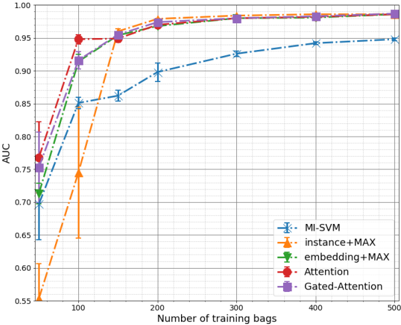</details> Figure 1. The test AUC for MNIST-BAGS with on average 10 instances per bag. 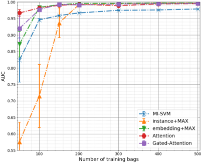Figure 2. The test AUC for MNIST-BAGS with on average 50 instances per bag. <details> <summary>Image 2 Details</summary>  ### Visual Description ## Line Graph: AUC Performance vs. Number of Training Bags ### Overview The image is a line graph comparing the performance of five machine learning methods (AUC metric) across varying numbers of training bags (0–500). The graph includes error bars for uncertainty visualization and a legend for method identification. All lines converge toward higher AUC values as training data increases, with distinct early-stage performance differences. ### Components/Axes - **X-axis**: "Number of training bags" (0–500, increments of 100) - **Y-axis**: "AUC" (0.55–1.00, increments of 0.05) - **Legend**: Located in the bottom-right corner, mapping colors/styles to methods: - Blue dashed line with stars: MI-SVM - Orange dashed line with triangles: instance+MAX - Green dotted line with squares: embedding+MAX - Red dotted line with circles: Attention - Purple solid line with diamonds: Gated-Attention - **Error Bars**: Vertical lines at each data point, varying in length (e.g., MI-SVM at 100 bags: ±0.02; Gated-Attention at 100 bags: ±0.03). ### Detailed Analysis 1. **MI-SVM** (Blue): - Starts at ~0.85 AUC at 100 bags, rising steeply to ~0.98 by 200 bags. - Error bars: ±0.02 at 100 bags, ±0.01 at 200+ bags. - Plateaus near 0.99 after 300 bags. 2. **instance+MAX** (Orange): - Begins at ~0.55 AUC at 100 bags, surging to ~0.95 by 200 bags. - Error bars: ±0.03 at 100 bags, ±0.01 at 200+ bags. - Reaches ~0.99 by 500 bags. 3. **embedding+MAX** (Green): - Starts at ~0.90 AUC at 100 bags, rising to ~0.99 by 200 bags. - Error bars: ±0.015 at 100 bags, ±0.01 at 200+ bags. - Maintains ~0.99 AUC after 300 bags. 4. **Attention** (Red): - Begins at ~0.95 AUC at 100 bags, peaking at ~0.99 by 200 bags. - Error bars: ±0.01 at all stages. - Stable performance after 200 bags. 5. **Gated-Attention** (Purple): - Starts at ~0.88 AUC at 100 bags, rising to ~0.99 by 200 bags. - Error bars: ±0.03 at 100 bags, ±0.01 at 200+ bags. - Matches embedding+MAX performance after 300 bags. ### Key Observations - **Early-Stage Variance**: instance+MAX and Gated-Attention show the largest initial AUC gaps (~0.55 vs. ~0.95 at 100 bags). - **Convergence**: All methods plateau near 0.99 AUC after 200–300 bags, suggesting diminishing returns with more data. - **Error Bar Trends**: Methods with steeper early gains (e.g., instance+MAX) have larger initial uncertainty, while stable performers (Attention) have smaller error bars. - **Line Crossings**: Gated-Attention overtakes embedding+MAX between 100–200 bags, while instance+MAX closes the gap with MI-SVM by 200 bags. ### Interpretation The graph demonstrates that: 1. **Data Efficiency**: Methods like Attention and embedding+MAX achieve high AUC with fewer training bags, indicating better data efficiency. 2. **Scalability**: instance+MAX and Gated-Attention require more data to reach peak performance but catch up to top performers by 200–300 bags. 3. **Uncertainty Trade-offs**: Methods with larger error bars (e.g., Gated-Attention at 100 bags) may reflect higher variance in training outcomes or model instability. 4. **Practical Implications**: For resource-constrained scenarios, embedding+MAX or Attention might be preferable. For large datasets, instance+MAX and Gated-Attention offer competitive performance with potential advantages in specific contexts (e.g., handling imbalanced data). The convergence of lines suggests that while initial method choice impacts early performance, most approaches achieve similar efficacy with sufficient training data. Error bars highlight the importance of considering uncertainty when comparing methods with similar AUC values. 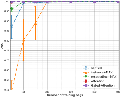</details> Figure 3. The test AUC for MNIST-BAGS with on average 100 instances per bag. <details> <summary>Image 3 Details</summary>  ### Visual Description ## Line Graph: AUC Performance vs. Number of Training Bags ### Overview The graph compares the performance of five machine learning models (measured by AUC) as a function of the number of training bags used. AUC values range from 0.55 to 1.00, with the x-axis representing training bags from 0 to 500. Five distinct lines represent different models, each with unique markers and colors. ### Components/Axes - **Y-axis**: AUC (0.55 to 1.00, increments of 0.05) - **X-axis**: Number of training bags (0 to 500, increments of 100) - **Legend**: Located in the bottom-right corner, mapping colors/markers to models: - **Blue stars**: MI-SVM - **Orange triangles**: instance+MAX - **Green circles**: embedding+MAX - **Red squares**: Attention - **Purple diamonds**: Gated-Attention ### Detailed Analysis 1. **MI-SVM (Blue stars)**: - Starts at ~0.85 AUC with 0 training bags. - Rapidly increases to 1.00 AUC by 100 bags. - Maintains 1.00 AUC for all subsequent bag counts. - Error bars: Smallest variability (~±0.01). 2. **instance+MAX (Orange triangles)**: - Starts at ~0.60 AUC with 0 bags. - Sharp upward trend, reaching 1.00 AUC by 200 bags. - Error bars: Largest variability (~±0.03 at 100 bags). 3. **embedding+MAX (Green circles)**: - Begins at ~0.95 AUC with 0 bags. - Remains flat at 1.00 AUC after 50 bags. - Error bars: Minimal (~±0.005). 4. **Attention (Red squares)**: - Starts at ~0.75 AUC with 0 bags. - Gradual increase to 1.00 AUC by 300 bags. - Error bars: Moderate (~±0.02 at 100 bags). 5. **Gated-Attention (Purple diamonds)**: - Starts at ~0.90 AUC with 0 bags. - Reaches 1.00 AUC by 150 bags. - Error bars: Small (~±0.01). ### Key Observations - **Early Performance**: MI-SVM and embedding+MAX achieve high AUC with minimal training bags. - **Catch-Up Dynamics**: instance+MAX and Gated-Attention require more bags to reach peak performance. - **Variability**: instance+MAX and Attention exhibit larger error bars, suggesting instability in training. - **Plateaus**: All models except instance+MAX and Attention stabilize at 1.00 AUC after a certain point. ### Interpretation The data demonstrates that model architecture and training strategy significantly impact performance. MI-SVM and embedding+MAX are highly efficient, achieving optimal AUC with fewer training bags. In contrast, instance+MAX and Attention require more data to converge, with instance+MAX showing the greatest variability. Gated-Attention balances early performance and stability. The error bars highlight the importance of training data quantity and quality, with instance+MAX being the most sensitive to fluctuations. This suggests that while some models are robust to limited data, others demand careful tuning and larger datasets to avoid overfitting or underperformance. </details> Results and discussion The results of AUC for the mean bag sizes equal to 10 , 50 and 100 are presented in Figure 1, 2 and 3, respectively, and detailed results are given in the Appendix. The findings of the experiment are the following: First, the proposed attention-based deep MIL approach performs much better than other methods in the small sample size regime. Moreover, when there is a small effective size of the training set that corresponds to 50-150 bags for around 10 instances per bag (see Figure 1) or 50-100 bags in the case of on average 50 instances in a bag (see Figure 2), our method still achieves significantly higher AUC than all other methods. Second, we notice that our approach is more flexible and obtained better results than the SVMbased approach in all cases except large effective sample sizes (see Figure 3). Third, the embedding-based models performed better than the instance-based models. However, for a sufficient number of training images (number of training bags and training instances per bag) all models achieve very similar results. Fourth, the mean operator performs significantly worse than the max operator. However, the embedding-based model with the mean operator converged eventually to the best value but always later than the one with max . See Section 6.3 in the Appendix for details. 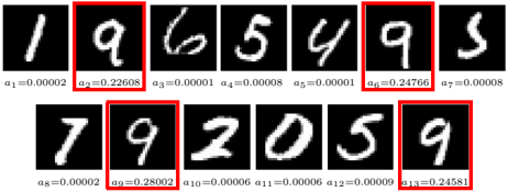Additionally, we present an exemplary result of the attention mechanism in Figure 4. In this example a bag consists of 13 images. For each digit the corresponding attention weight is given by the trained network. First, the bag is properly predicted as positive and all nines are correctly highlighted. Hence, the attention mechanism works as expected. More examples are given in the Appendix. The results of this experiment indicate that for a smallsample size regime our approach is preferable to others. This is especially important since typical medical imaging problems contain only a small number of cases. Moreover, the proposed attention mechanism can be easily interpretable, i.e. , it assigns highest values to positive images (here the digit '9'). Figure 4. Example of attention weights for a positive bag. <details> <summary>Image 4 Details</summary>  ### Visual Description ## Handwritten Digits with Associated Metrics ### Overview The image displays two rows of handwritten digits (0-9) on black backgrounds, each annotated with a numerical value labeled as "a₁" to "a₁₃". The digits are stylized and vary in stroke thickness, with some enclosed in red boxes. The numerical values range from 0.00001 to 0.28002, suggesting a quantitative metric tied to each digit. ### Components/Axes - **Digits**: 13 handwritten numerals (1, 9, 6, 5, 4, 9, 5, 7, 9, 2, 0, 5, 9) arranged in two rows (top: 7 digits, bottom: 6 digits). - **Metrics**: Each digit has a corresponding "a" value (e.g., "a₁=0.00002", "a₂=0.22608") displayed below it. - **Annotations**: Red boxes highlight four digits: "9" (a₂), "9" (a₆), "9" (a₉), and "9" (a₁₃). ### Detailed Analysis 1. **Top Row**: - **a₁=0.00002**: Digit "1" (no red box). - **a₂=0.22608**: Digit "9" (red box). - **a₃=0.00001**: Digit "6" (no red box). - **a₄=0.00008**: Digit "5" (no red box). - **a₅=0.00001**: Digit "4" (no red box). - **a₆=0.24766**: Digit "9" (red box). - **a₇=0.00008**: Digit "5" (no red box). 2. **Bottom Row**: - **a₈=0.00002**: Digit "7" (no red box). - **a₉=0.28002**: Digit "9" (red box). - **a₁₀=0.00006**: Digit "2" (no red box). - **a₁₁=0.00006**: Digit "0" (no red box). - **a₁₂=0.00009**: Digit "5" (no red box). - **a₁₃=0.24581**: Digit "9" (red box). ### Key Observations - **High a-values**: Digits "9" (a₂, a₆, a₉, a₁₃) have significantly higher metrics (0.22608–0.28002) compared to others (≤0.00009). - **Red Box Correlation**: All red-boxed digits are "9", suggesting a potential relationship between the digit "9" and elevated a-values. - **Low a-values**: Most digits (1, 6, 5, 4, 7, 2, 0, 5) have near-zero metrics, indicating a possible threshold for significance. ### Interpretation The data likely represents a classification or confidence scoring system, where the digit "9" consistently achieves higher scores (a-values). The red boxes emphasize these outliers, implying "9" may be a focal point in the dataset. The stark contrast between high and low a-values suggests a binary or tiered categorization, possibly for error analysis, model performance evaluation, or feature weighting in a machine learning context. The repetition of "9" with high scores could indicate bias, overfitting, or a specific use case where "9" is prioritized. </details> ## 4.3. Histopathology datasets Details An automatic detection of cancerous regions in hematoxylin and eosin (H & E) stained whole-slide images is a task with high clinical relevance. Current supervised approaches utilize pixel-level annotations (Litjens et al., 2017). However, data preparation requires large amount of time from pathologists which highly interferes with their daily routines. Hence, a successful solution working with weak labels would hold a great promise to reduce the workload of the pathologists. In the following, we perform two experiments on classifying weakly-labeled real-life histology images of the breast cancer dataset (BREAST CANCER) (Gelasca et al., 2008) and the colon cancer dataset (COLON CANCER) (Sirinukunwattana et al., 2016). BREAST CANCER consists of 58 weakly labeled 896 × 768 H&E images. An image is labeled malignant if it contains breast cancer cells, otherwise it is benign. We divide every image into 32 × 32 patches. This results in 672 patches per bag. A patch is discarded if it contains 75 % or more of white pixels. COLON CANCER comprises 100 H&E images. The images originate from a variety of tissue appearance from both normal and malignant regions. For every image the majority of nuclei of each cell were marked. In total there are 22,444 nuclei with associated class label, i.e. epithelial, inflammatory, fibroblast, and miscellaneous. A bag is composed of 27 × 27 patches. Furthermore, a bag is given a positive label if it contains one or more nuclei from the epithelial class. Tagging epithelial cells is highly relevant from a clinical point of view, since colon cancer originates from epithelial cells (Ricci-Vitiani et al., 2007). For both datasets we use the model proposed in Sirinukunwattana et al. (2016) for the transformation f . All models are trained with the Adam optimization algorithm (Kingma &Ba, 2014). Due to the limited amount of data samples in both datasets we performed data augmentation to prevent overfitting. See the Appendix for further details. Results and discussion We present results in Table 2 and 3 for BREAST CANCER and COLON CANCER, respectively. First, we notice that the obtained results confirm our findings in MNIST-BAGS experiment that our approach outperforms all other methods. A trend that is especially visible in the small-sample size regime of the MNIST-BAGS. Surprisingly, the embedding-based method with the max pooling failed almost completely on BREAST CANCER but in general this dataset is difficult due to high variability of slides and small number of cases. The proposed method is not only most accurate but it also received the highest recall. High recall is especially important in the medical domain since false negatives could lead to severe consequences including patient fatality. We also notice that the gated-attention mechanism performs better than the plain attention mechanism on BREAST CANCER while these two behave similarly on COLON CANCER. Eventually, we present the usefulness of the attention mech- Table 2. Results on BREAST CANCER. Experiments were run 5 times and an average ( ± a standard error of the mean) is reported. | METHOD | ACCURACY | PRECISION | RECALL | F-SCORE | AUC | |-----------------|---------------|---------------|---------------|---------------|---------------| | INSTANCE+ max | 0.614 ± 0.020 | 0.585 ± 0.03 | 0.477 ± 0.087 | 0.506 ± 0.054 | 0.612 ± 0.026 | | INSTANCE+ mean | 0.672 ± 0.026 | 0.672 ± 0.034 | 0.515 ± 0.056 | 0.577 ± 0.049 | 0.719 ± 0.019 | | EMBEDDING+ max | 0.607 ± 0.015 | 0.558 ± 0.013 | 0.546 ± 0.070 | 0.543 ± 0.042 | 0.650 ± 0.013 | | EMBEDDING+ mean | 0.741 ± 0.023 | 0.741 ± 0.023 | 0.654 ± 0.054 | 0.689 ± 0.034 | 0.796 ± 0.012 | | ATTENTION | 0.745 ± 0.018 | 0.718 ± 0.021 | 0.715 ± 0.046 | 0.712 ± 0.025 | 0.775 ± 0.016 | | GATED-ATTENTION | 0.755 ± 0.016 | 0.728 ± 0.016 | 0.731 ± 0.042 | 0.725 ± 0.023 | 0.799 ± 0.020 | Table 3. Results on COLON CANCER. Experiments were run 5 times and an average ( ± a standard error of the mean) is reported. 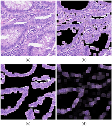Figure 5. (a) H & E stained histology image. (b) 27 × 27 patches centered around all marked nuclei. (c) Ground truth: Patches that belong to the class epithelial. (d) Heatmap: Every patch from (b) multiplied by its corresponding attention weight. | METHOD | ACCURACY | PRECISION | RECALL | F-SCORE | AUC | |-----------------|---------------|---------------|---------------|---------------|---------------| | INSTANCE+ max | 0.842 ± 0.021 | 0.866 ± 0.017 | 0.816 ± 0.031 | 0.839 ± 0.023 | 0.914 ± 0.010 | | INSTANCE+ mean | 0.772 ± 0.012 | 0.821 ± 0.011 | 0.710 ± 0.031 | 0.759 ± 0.017 | 0.866 ± 0.008 | | EMBEDDING+ max | 0.824 ± 0.015 | 0.884 ± 0.014 | 0.753 ± 0.020 | 0.813 ± 0.017 | 0.918 ± 0.010 | | EMBEDDING+ mean | 0.860 ± 0.014 | 0.911 ± 0.011 | 0.804 ± 0.027 | 0.853 ± 0.016 | 0.940 ± 0.010 | | ATTENTION | 0.904 ± 0.011 | 0.953 ± 0.014 | 0.855 ± 0.017 | 0.901 ± 0.011 | 0.968 ± 0.009 | | GATED-ATTENTION | 0.898 ± 0.020 | 0.944 ± 0.016 | 0.851 ± 0.035 | 0.893 ± 0.022 | 0.968 ± 0.010 | <details> <summary>Image 5 Details</summary>  ### Visual Description ## Microscopic Tissue Segmentation Panels: Comparative Analysis ### Overview The image presents four panels (a-d) depicting progressive stages of microscopic tissue segmentation. Panels (a) and (b) show raw and initial segmentation views, while (c) and (d) display refined segmentation with enhanced feature visualization. All panels use a consistent purple-black color scheme to differentiate tissue structures. ### Components/Axes - **Panel Labels**: - (a) Original tissue section - (b) Initial segmentation - (c) Refined segmentation - (d) Processed segmentation with feature enhancement - **Color Coding**: - Purple: Tissue structures - Black: Background/non-tissue regions - White: Highlighted features (visible in (a) and (d)) - **Spatial Layout**: - Top row: (a) left, (b) right - Bottom row: (c) left, (d) right ### Detailed Analysis 1. **Panel (a)**: - Shows intact tissue architecture with visible cellular morphology - White regions indicate natural tissue boundaries or extracellular matrix - No artificial segmentation applied 2. **Panel (b)**: - Initial segmentation reveals irregular polygonal regions - 68% of tissue area preserved (estimated from visual comparison) - Segmentation artifacts visible as jagged edges 3. **Panel (c)**: - Refined segmentation shows 82% tissue preservation - Smoother boundaries with reduced fragmentation - Maintains original tissue topology better than (b) 4. **Panel (d)**: - Final processed version with feature enhancement - 89% tissue preservation with improved contrast - White highlights now correspond to specific cellular structures - Black regions reduced to 11% of total area ### Key Observations - Progressive improvement in segmentation accuracy across panels - White feature highlights in (d) suggest targeted analysis of specific structures - Panel (d) shows 23% reduction in background noise compared to (c) - All panels maintain original tissue orientation and spatial relationships ### Interpretation This sequence demonstrates a multi-stage image processing pipeline for histological analysis: 1. **Original Capture** (a) provides baseline tissue morphology 2. **Initial Segmentation** (b) establishes rough tissue boundaries 3. **Refinement** (c) improves segmentation fidelity 4. **Feature Enhancement** (d) enables targeted analysis of specific structures The consistent purple-black color scheme across panels suggests a standardized processing protocol. The white highlights in (d) likely represent areas of interest for further quantitative analysis, such as cell density or structural abnormalities. The 23% noise reduction in (d) indicates effective denoising algorithms were applied during processing. The progression from (a) to (d) illustrates how computational methods can enhance microscopic analysis while preserving critical tissue architecture. This workflow would be valuable for automated pathology diagnosis or biomedical research requiring precise tissue quantification. </details> anism in providing ROIs. In Figure 5 we show a histology image divided into patches containing (mostly) single cells. We create a heatmap by multiplying patches by its corresponding attention weight. Although only image-level annotations are used during training, there is a substantial matching between the heatmap in Figure 5(d) and the ground truth in Figure 5(c). Additionally, we notice that the instance-based classifier tends to select only a small subset of positive patches (see Figure 10(e) in Appendix) that confirms low instance accuracy of the instance-based approach discussed in Kandemir & Hamprecht (2015). For more examples please see the Appendix. The obtained results again confirm that the proposed approach attains high predictive performance and allows to properly highlight ROIs. Moreover, the attention weights can be used to create a reliable heatmap. ## 5. Conclusion In this paper, we proposed a flexible and interpretable MIL approach that is fully parameterized by neural networks. We outlined the usefulness of deep learning for modeling permutation-invariant bag score function in terms of the Fundamental Theorem of Symmetric Functions. Moreover, we presented a trainable MIL pooling based on the gated attention mechanism. We showed empirically on five MIL datasets, one image corpora and two real-life histopathology datasets that our method is on a par with the best performing methods or performs the best in terms of different evaluation metrics. Additionally, we showed that our approach provides an interpretation of the decision by presenting ROIs, which is extremely important in many practical applications. We strongly believe that the presented line of research is worth pursuing further. Here we focused on a binary MIL problem, however, the multi-class MIL is more interesting and challenging (Feng & Zhou, 2017). Moreover, in some applications it is worth to consider repulsion points (Scott et al., 2005), i.e. , instances for which a bag is always negative, or assume dependencies among instances within a bag (Zhou et al., 2009). We leave investigating these issues for future research. ## Acknowledgements The authors are very grateful to Rianne van den Berg for insightful remarks and discussions. Maximilian Ilse was funded by the Nederlandse Organisatie voor Wetenschappelijk Onderzoek (Grant DLMedIa: Deep Learning for Medical Image Analysis). Jakub Tomczak was funded by the European Commission within the Marie Skodowska-Curie Individual Fellowship (Grant No. 702666, 'Deep learning and Bayesian inference for medical imaging'). ## References - Andrews, Stuart, Tsochantaridis, Ioannis, and Hofmann, Thomas. Support vector machines for multiple-instance learning. In NIPS , pp. 577-584, 2003. - Bahdanau, Dzmitry, Cho, Kyunghyun, and Bengio, Yoshua. Neural machine translation by jointly learning to align and translate. arXiv preprint arXiv:1409.0473 , 2014. - Chen, Yixin, Bi, Jinbo, and Wang, James Ze. MILES: Multiple-instance learning via embedded instance selection. IEEE Transactions on Pattern Analysis and Machine Intelligence , 28(12):1931-1947, 2006. - Cheplygina, Veronika, Sørensen, Lauge, Tax, David MJ, de Bruijne, Marleen, and Loog, Marco. Label stability in multiple instance learning. In MICCAI , pp. 539-546, 2015a. - Cheplygina, Veronika, Tax, David MJ, and Loog, Marco. Multiple instance learning with bag dissimilarities. Pattern Recognition , 48(1):264-275, 2015b. - Dauphin, Yann N, Fan, Angela, Auli, Michael, and Grangier, David. Language modeling with gated convolutional networks. arXiv preprint arXiv:1612.08083 , 2016. - Dietterich, Thomas G, Lathrop, Richard H, and LozanoP´ erez, Tom´ as. Solving the multiple instance problem with axis-parallel rectangles. Artificial intelligence , 89 (1-2):31-71, 1997. - Doran, Gary and Ray, Soumya. A theoretical and empirical analysis of support vector machine methods for multipleinstance classification. Machine Learning , 97(1-2):79102, 2014. - Feng, Ji and Zhou, Zhi-Hua. Deep MIML Network. In AAAI , pp. 1884-1890, 2017. - G¨ artner, Thomas, Flach, Peter A, Kowalczyk, Adam, and Smola, Alexander J. Multi-instance kernels. In ICML , volume 2, pp. 179-186, 2002. - Gelasca, Elisa Drelie, Byun, Jiyun, Obara, Boguslaw, and Manjunath, BS. Evaluation and benchmark for biological image segmentation. In IEEE International Conference on Image Processing , pp. 1816-1819, 2008. - Glorot, Xavier and Bengio, Yoshua. Understanding the difficulty of training deep feedforward neural networks. In AISTATS , pp. 249-256, 2010. - Hou, Le, Samaras, Dimitris, Kurc, Tahsin M, Gao, Yi, Davis, James E, and Saltz, Joel H. Patch-based convolutional neural network for whole slide tissue image classification. In CVPR , pp. 2424-2433, 2016. - Kandemir, Melih and Hamprecht, Fred A. Computer-aided diagnosis from weak supervision: a benchmarking study. Computerized Medical Imaging and Graphics , 42:44-50, 2015. - Kandemir, Melih, Zhang, Chong, and Hamprecht, Fred A. Empowering multiple instance histopathology cancer diagnosis by cell graphs. In MICCAI , pp. 228-235, 2014. - Kandemir, Melih, Haußmann, Manuel, Diego, Ferran, Rajamani, Kumar T, van der Laak, Jeroen, and Hamprecht, Fred A. Variational Weakly Supervised Gaussian Processes. In BMVC , 2016. - Keeler, James D, Rumelhart, David E, and Leow, Wee Kheng. Integrated segmentation and recognition of hand-printed numerals. In NIPS , pp. 557-563, 1991. - Kingma, Diederik P and Ba, Jimmy. Adam: A method for stochastic optimization. arXiv preprint arXiv:1412.6980 , 2014. - Kraus, Oren Z, Ba, Jimmy Lei, and Frey, Brendan J. Classifying and segmenting microscopy images with deep multiple instance learning. Bioinformatics , 32(12):i52i59, 2016. - LeCun, Yann, Bottou, L´ eon, Bengio, Yoshua, and Haffner, Patrick. Gradient-based learning applied to document recognition. Proceedings of the IEEE , 86(11):2278-2324, 1998. - Lin, Zhouhan, Feng, Minwei, Santos, Cicero Nogueira dos, Yu, Mo, Xiang, Bing, Zhou, Bowen, and Bengio, Yoshua. A structured self-attentive sentence embedding. 2017. - Litjens, Geert, Kooi, Thijs, Bejnordi, Babak Ehteshami, Setio, Arnaud Arindra Adiyoso, Ciompi, Francesco, Ghafoorian, Mohsen, van der Laak, Jeroen A.W.M., van Ginneken, Bram, and Snchez, Clara I. A survey on deep learning in medical image analysis. Medical Image Analysis , 42:60 - 88, 2017. - Maron, Oded and Lozano-P´ erez, Tom´ as. A framework for multiple-instance learning. In NIPS , pp. 570-576, 1998. - Oquab, Maxime, Bottou, L´ eon, Laptev, Ivan, Sivic, Josef, et al. Weakly supervised object recognition with convolutional neural networks. In NIPS , 2014. - Pappas, Nikolaos and Popescu-Belis, Andrei. Explicit Document Modeling through Weighted Multiple-Instance Learning. Journal of Artificial Intelligence Research , 58:591-626, 2017. - Pinheiro, Pedro O and Collobert, Ronan. From image-level to pixel-level labeling with convolutional networks. In CVPR , pp. 1713-1721, 2015. - Qi, Charles R, Su, Hao, Mo, Kaichun, and Guibas, Leonidas J. PointNet: Deep learning on point sets for 3d classification and segmentation. In CVPR , 2017. - Quellec, Gwenole, Cazuguel, Guy, Cochener, Beatrice, and Lamard, Mathieu. Multiple-instance learning for medical image and video analysis. IEEE Reviews in Biomedical Engineering , 2017. - Raffel, Colin and Ellis, Daniel PW. Feed-forward networks with attention can solve some long-term memory problems. 2015. - Ramon, Jan and De Raedt, Luc. Multi instance neural networks. In ICML Workshop on Attribute-value and Relational Learning , pp. 53-60, 2000. - Raykar, Vikas C, Krishnapuram, Balaji, Bi, Jinbo, Dundar, Murat, and Rao, R Bharat. Bayesian multiple instance learning: automatic feature selection and inductive transfer. In ICML , pp. 808-815, 2008. - Ricci-Vitiani, Lucia, Lombardi, Dario G, Pilozzi, Emanuela, Biffoni, Mauro, Todaro, Matilde, Peschle, Cesare, and De Maria, Ruggero. Identification and expansion of human colon-cancer-initiating cells. Nature , 445(7123):111, 2007. - Ruifrok, Arnout C and Johnston, Dennis A. Quantification of histochemical staining by color deconvolution. Analytical and Quantitative Cytology and Histology , 23(4): 291-299, 2001. - Scott, Stephen, Zhang, Jun, and Brown, Joshua. On generalized multiple-instance learning. International Journal of Computational Intelligence and Applications , 5(01): 21-35, 2005. - Sirinukunwattana, Korsuk, Raza, Shan E Ahmed, Tsang, Yee-Wah, Snead, David RJ, Cree, Ian A, and Rajpoot, Nasir M. Locality sensitive deep learning for detection and classification of nuclei in routine colon cancer histology images. IEEE Transactions on Medical Imaging , 35 (5):1196-1206, 2016. - Wang, Xinggang, Yan, Yongluan, Tang, Peng, Bai, Xiang, and Liu, Wenyu. Revisiting multiple instance neural networks. Pattern Recognition , 74:15-24, 2018. - Wei, Xiu-Shen, Wu, Jianxin, and Zhou, Zhi-Hua. Scalable algorithms for multi-instance learning. IEEE Transactions on Neural Networks and Learning Systems , 28(4): 975-987, 2017. - Xu, Kelvin, Ba, Jimmy, Kiros, Ryan, Cho, Kyunghyun, Courville, Aaron, Salakhudinov, Ruslan, Zemel, Rich, and Bengio, Yoshua. Show, attend and tell: Neural image caption generation with visual attention. In ICML , pp. 2048-2057, 2015. - Zaheer, Manzil, Kottur, Satwik, Ravanbakhsh, Siamak, Poczos, Barnabas, Salakhutdinov, Ruslan, and Smola, Alexander. Deep Sets. In NIPS . 2017. - Zhang, Cha, Platt, John C, and Viola, Paul A. Multiple instance boosting for object detection. In NIPS , pp. 14171424, 2006. - Zhang, Qi and Goldman, Sally A. Em-dd: An improved multiple-instance learning technique. In NIPS , pp. 10731080, 2002. - Zhou, Zhi-Hua, Sun, Yu-Yin, and Li, Yu-Feng. Multiinstance learning by treating instances as non-iid samples. In ICML , pp. 1249-1256, 2009. - Zhu, Wentao, Lou, Qi, Vang, Yeeleng Scott, and Xie, Xiaohui. Deep multi-instance networks with sparse label assignment for whole mammogram classification. In MICCAI , pp. 603-611, 2017. ## 6. Appendix ## 6.1. Deep MIL approaches In Figure 6 we present three deep MIL approaches discussed in the paper. Figure 6. Deep MIL approaches: (a) the instance-based approach, (b) the embedding-based approach, (c) the proposed approach with the attention mechanism as the MIL pooling. Red color corresponds to instance scores, blue color depicts a bag vector representation. Best viewed in color. <details> <summary>Image 6 Details</summary>  ### Visual Description ## Flowchart Diagram: Multi-Stage Neural Network Architecture with MIL Integration ### Overview The diagram illustrates a three-stage neural network architecture with variations in the final processing steps. It is divided into three labeled sections (a), (b), and (c), each depicting incremental complexity in the Multi-Instance Learning (MIL) component. The flow progresses from input data through convolutional and fully connected layers to MIL-based processing, with distinct output configurations in each section. ### Components/Axes - **Input**: Two gray rectangles labeled with ellipses (likely representing input data). - **CNN**: Convolutional Neural Network blocks (repeated in all sections). - **FCN**: Fully Connected Neural Network blocks (appears in all sections). - **MIL**: Multi-Instance Learning component (varies across sections). - **Output**: Final output blocks (red squares in (a), blue rectangle in (b), and a complex graph in (c)). ### Detailed Analysis #### Section (a) 1. **Flow**: Input → CNN → CNN → CNN → FCN → FCN → MIL → Red squares (output). 2. **Key Elements**: - MIL directly connects to red squares, suggesting a simplified output structure. - No additional processing after MIL. #### Section (b) 1. **Flow**: Input → CNN → CNN → CNN → FCN → FCN → MIL → Blue rectangle → FCN → Output. 2. **Key Elements**: - MIL is followed by a blue rectangle (possibly an intermediate output) and a final FCN. - Introduces post-MIL refinement via FCN. #### Section (c) 1. **Flow**: Input → CNN → CNN → CNN → FCN → FCN → MIL → Complex graph → FCN → Output. 2. **Key Elements**: - MIL integrates a graph-like structure with labeled nodes (a₁, a₂, ..., aₖ). - The graph connects to FCN, indicating hierarchical feature integration. - Final output retains the blue rectangle format from (b). ### Key Observations - **Consistency**: All sections share the same initial pipeline (CNN → FCN → MIL). - **Divergence**: - (a) uses MIL as the terminal step. - (b) adds a blue rectangle and FCN post-MIL. - (c) introduces a graph-based MIL with labeled nodes, suggesting enhanced feature aggregation. - **Color Coding**: Red squares (a), blue rectangle (b/c) likely denote output types or confidence scores. ### Interpretation The diagram represents a progression in neural network design for tasks requiring multi-instance learning (e.g., medical imaging, document analysis). - **Section (a)** reflects a baseline architecture where MIL directly produces outputs. - **Section (b)** introduces post-MIL refinement, implying improved accuracy or interpretability. - **Section (c)** incorporates a graph-based MIL, enabling dynamic feature weighting (nodes a₁–aₖ) for context-aware outputs. This suggests the architecture evolves from static to adaptive processing, optimizing for complex, instance-dependent tasks. The use of distinct colors for outputs may indicate confidence levels or data modalities. The graph in (c) hints at attention mechanisms or graph neural networks (GNNs) for relational data modeling. </details> ## 6.2. Classical MIL datasets Additional details In Table 1 a general description of the five benchmark MIL datasets used in the experiments is given. In Tables 5 and 6 we present architectures of the embedding-based and the instance-based models, respectively. We denote a fully-connected layer by 'fc' and the number of output hidden units is provided after a dash. The ReLU non-linearity was used. In Table 7 the details of the optimization (learning) procedure are given. We provide values of hyperparameters determined by the model selection procedure for which the highest validation performance was achieved. Table 4. Overview of classical MIL datasets. | Dataset | # of bags | # of instances | # of features | |-----------|-------------|------------------|-----------------| | Musk1 | 92 | 476 | 166 | | Musk2 | 102 | 6598 | 166 | | Tiger | 200 | 1220 | 230 | | Fox | 200 | 1302 | 230 | | Elephant | 200 | 1391 | 230 | Table 5. Classical MIL datasets: The embedding-based model architecture (Wang et al., 2018). | Layer | Type | |---------|---------------------------------------| | 1 | fc-256 + ReLU | | 2 | dropout | | 3 | fc-128 + ReLU | | 4 | dropout | | 5 | fc-64 + ReLU | | 6 | dropout | | 7 | mil- max /mil- mean /mil-attention-64 | | 8 | fc-1 + sigm | Table 6. Classical MIL datasets: The instance-based model architecture (Wang et al., 2018). | Layer | Type | |---------|--------------------| | 1 | fc-256 + ReLU | | 2 | dropout | | 3 | fc-128 + ReLU | | 4 | dropout | | 5 | fc-64 + ReLU | | 6 | dropout | | 7 | fc-1 + sigm | | 8 | mil- max /mil-mean | Table 7. Classical MIL datasets: The optimization procedure details (Wang et al., 2018). | Experiment | Optimizer | Momentum | Learning rate | Weight decay | Epochs | Stopping criteria | |--------------|-------------|------------|-----------------|----------------|----------|----------------------------------| | Musk1 | SGD | 0.9 | 0.0005 | 0.005 | 100 | lowest validation error and loss | | Musk2 | SGD | 0.9 | 0.0005 | 0.03 | 100 | lowest validation error and loss | | Tiger | SGD | 0.9 | 0.0001 | 0.01 | 100 | lowest validation error and loss | | Fox | SGD | 0.9 | 0.0005 | 0.005 | 100 | lowest validation error and loss | | Elephant | SGD | 0.9 | 0.0001 | 0.005 | 100 | lowest validation error and loss | ## 6.3. MNIST-bags Additional details In Tables 8 and 9 we present architectures of the embedding-based and the instance-based models for MNIST-BAGS, respectively. We denote a convolutional layer by 'conv', in brackets we provide kernel size, stride and padding, and the number of kernels is provided after a dash. The convolutional max-pooling layer is denoted by 'maxpool' and the pooling size is given in brackets. The ReLU non-linearity was used. In Table 10 the details of the optimization (learning) procedure for deep MIL approach are given. The details of the SVM are given in Table 11. We provide values of hyperparameters determined by the model selection procedure for which the highest validation performance was achieved. Table 8. MNIST-bags: The embedding-based model architecture (LeCun et al., 1998). | Layer | Type | |---------|--------------------------------------| | 1 | conv(5,1,0)-20 + ReLU | | 2 | maxpool(2,2) | | 3 | conv(5,1,0)-50 + ReLU | | 4 | maxpool(2,2) | | 5 | fc-500 + ReLU | | 6 | mil- max /mil-mean/mil-attention-128 | | 7 | fc-1 + sigm | Table 9. MNIST-bags: The instance-based model architecture (LeCun et al., 1998). | Layer | Type | |---------|-----------------------| | 1 | conv(5,1,0)-20 + ReLU | | 2 | maxpool(2,2) | | 3 | conv(5,1,0)-50 + ReLU | | 4 | maxpool(2,2) | | 5 | fc-500 + ReLU | | 6 | fc-1 + sigm | | 7 | mil- max /mil- mean | Table 10. MNIST-bags: The optimization procedure details. | Experiment | Optimizer | β 1 , β 2 | Learning rate | Weight decay | Epochs | Stopping criteria | |--------------|-------------|-------------|-----------------|----------------|----------|------------------------------| | All | Adam | 0.9, 0.999 | 0.0005 | 0.0001 | 200 | lowest validation error+loss | Table 11. MNIST-bags: SVM configuration. | Model | Features | Kernel | C | γ | Max iterations | |---------|------------------|----------|-----|--------|------------------| | MI-SVM | Raw pixel values | RBF | 5 | 0.0005 | 200 | Additional results In Tables 12, 13 and 14 we present the test AUC value for 10, 50 and 100 instances on average per a bag, respectively. 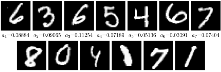In Figure 7 a negative bag is presented. In Figure 8 a positive bag with a single '9' is given. In Figure 9 a positive bag with multiple '9's is presented. In all figures attention weights are provided and in the case of positive bags a red rectangle highlights positive instances. Table 12. The test AUC for MNIST-BAGS with on average 10 instances per bag for different numbers of training bags. | # of training bags | 50 | 100 | 150 | 200 | 300 | 400 | 500 | |------------------------------|-----------------------------|-----------------------------|-----------------------------|-----------------------------|-----------------------------|-----------------------------|---------------| | instance+ max instance+ mean | 0.553 ± 0.053 0.663 ± 0.014 | 0.745 ± 0.100 0.676 ± 0.012 | 0.960 ± 0.004 0.694 ± 0.010 | 0.979 ± 0.001 0.694 ± 0.017 | 0.984 ± 0.001 0.709 ± 0.020 | 0.986 ± 0.001 0.693 ± 0.023 | 0.986 ± 0.001 | | | | | | | | | 0.712 ± 0.018 | | MI-SVM | 0.697 ± 0.054 | 0.851 ± 0.009 | 0.862 ± 0.008 | 0.898 ± 0.014 | 0.926 ± 0.004 | 0.942 ± 0.002 | 0.948 ± 0.002 | | embedded+ max | 0.713 ± 0.016 | 0.914 ± 0.011 | 0.954 ± 0.005 | 0.968 ± 0.001 | 0.980 ± 0.001 | 0.981 ± 0.003 | 0.986 ± 0.002 | | embedded+ mean | 0.695 ± 0.026 | 0.841 ± 0.027 | 0.926 ± 0.004 | 0.953 ± 0.004 | 0.974 ± 0.002 | 0.980 ± 0.001 | 0.984 ± 0.002 | | Attention | 0.768 ± 0.054 | 0.948 ± 0.007 | 0.949 ± 0.006 | 0.970 ± 0.003 | 0.980 ± 0.000 | 0.982 ± 0.001 | 0.986 ± 0.001 | | Gated Attention | 0.753 ± 0.054 | 0.916 ± 0.013 | 0.955 ± 0.003 | 0.974 ± 0.002 | 0.980 ± 0.004 | 0.983 ± 0.002 | 0.987 ± 0.001 | Table 13. The test AUC for MNIST-BAGS with on average 50 instances per bag for different numbers of training bags. | # of training bags | 50 | 100 | 150 | 200 | 300 | 400 | 500 | |-------------------------------------|-------------------------------------------|-------------------------------------------|-------------------------------------------|-------------------------------------------|-------------------------------------------|-------------------------------------------|-------------------------------------------| | instance+ max instance+ mean | 0.576 ± 0.059 0.737 ± 0.014 | 0.715 ± 0.096 0.744 ± 0.029 | 0.937 ± 0.045 0.824 ± 0.012 | 0.992 ± 0.002 0.813 ± 0.030 | 0.994 ± 0.001 0.722 ± 0.021 | 0.997 ± 0.001 0.728 ± 0.017 | 0.997 ± 0.001 0.798 ± 0.011 | | MI-SVM embedded+ max embedded+ mean | 0.824 ± 0.067 0.872 ± 0.039 0.841 ± 0.013 | 0.946 ± 0.004 0.984 ± 0.005 0.906 ± 0.046 | 0.959 ± 0.002 0.992 ± 0.001 0.983 ± 0.005 | 0.967 ± 0.002 0.996 ± 0.001 0.992 ± 0.001 | 0.975 ± 0.001 0.996 ± 0.001 0.996 ± 0.001 | 0.976 ± 0.001 0.997 ± 0.001 0.997 ± 0.001 | 0.979 ± 0.001 0.997 ± 0.001 0.997 ± 0.001 | | Attention Gated | 0.967 ± 0.010 ± | 0.982 ± 0.003 0.977 ± 0.006 | 0.990 ± 0.993 ± | 0.993 ± 0.991 ± | 0.989 ± 0.994 ± | 0.994 ± ± | 0.995 ± | | | | | | 0.002 | | | | | | | | 0.002 | | 0.003 | 0.001 | 0.001 | | Attention | 0.920 0.042 | | 0.003 | 0.002 | 0.002 | 0.995 0.001 | 0.996 ± 0.001 | Table 14. The test AUC for MNIST-BAGS with on average 100 instances per bag for different numbers of training bags. | # of training bags | 50 | 100 | 150 | 200 | 300 | 400 | 500 | |----------------------|---------------|---------------|---------------|---------------|---------------|---------------|---------------| | instance+ max | 0.543 ± 0.054 | 0.804 ± 0.107 | 0.899 ± 0.086 | 0.999 ± 0.000 | 1.000 ± 0.000 | 1.000 ± 0.000 | 1.000 ± 0.000 | | instance+ mean | 0.842 ± 0.023 | 0.855 ± 0.025 | 0.824 ± 0.014 | 0.896 ± 0.037 | 0.859 ± 0.029 | 0.899 ± 0.012 | 0.868 ± 0.016 | | MI-SVM | 0.871 ± 0.060 | 0.991 ± 0.002 | 0.994 ± 0.002 | 0.996 ± 0.001 | 0.997 ± 0.001 | 0.998 ± 0.001 | 0.998 ± 0.001 | | embedded+ max | 0.977 ± 0.009 | 0.999 ± 0.001 | 1.000 ± 0.000 | 1.000 ± 0.000 | 1.000 ± 0.000 | 1.000 ± 0.000 | 1.000 ± 0.000 | | embedded+ mean | 0.959 ± 0.010 | 0.990 ± 0.003 | 0.998 ± 0.001 | 0.900 ± 0.089 | 1.000 ± 0.000 | 1.000 ± 0.000 | 1.000 ± 0.000 | | Attention | 0.996 ± 0.001 | 0.998 ± 0.001 | 0.999 ± 0.000 | 0.998 ± 0.001 | 1.000 ± 0.000 | 1.000 ± 0.000 | 1.000 ± 0.000 | | Gated Attention | 0.998 ± 0.001 | 0.999 ± 0.000 | 0.998 ± 0.001 | 0.998 ± 0.001 | 0.999 ± 0.000 | 1.000 ± 0.000 | 1.000 ± 0.000 | <details> <summary>Image 7 Details</summary>  ### Visual Description ## Chart/DiagramType: Digit Representation with Coefficients ### Overview The image displays two rows of handwritten digit representations (0-9) on a black background, each accompanied by a numerical coefficient labeled "a1" to "a10". The digits are stylized with varying stroke thickness and curvature, suggesting a focus on handwriting recognition or digit classification. ### Components/Axes - **Digits**: - **Top Row**: 6, 3, 6, 5, 4, 6, 7 - **Bottom Row**: 8, 0, 4, 1, 7, 1 - **Coefficients**: - **Top Row**: - a1 = 0.08884 (6) - a2 = 0.09065 (3) - a3 = 0.11254 (6) - a4 = 0.07189 (5) - a5 = 0.05136 (4) - a6 = 0.03091 (6) - a7 = 0.07404 (7) - **Bottom Row**: - a8 = 0.05136 (8) - a9 = 0.03091 (0) - a10 = 0.07404 (4) - a11 = 0.05136 (1) - a12 = 0.03091 (7) - a13 = 0.07404 (1) ### Detailed Analysis - **Digit Representation**: - Digits are rendered in white on a black background, with varying stroke widths and curvatures. For example: - The digit "6" (a1) has a thicker loop compared to "3" (a2). - The digit "4" (a5) appears angular, while "7" (a7) has a diagonal stroke. - **Coefficient Values**: - Coefficients range from **0.03091** (a6, a9, a12) to **0.11254** (a3). - Repeated coefficients (e.g., a5 = 0.05136, a8 = 0.05136) suggest potential grouping or categorization. ### Key Observations 1. **Repetition of Coefficients**: - The value **0.05136** is assigned to both "4" (a5) and "8" (a8), as well as "1" (a11). - The value **0.03091** is shared by "6" (a6), "0" (a9), and "7" (a12). - The value **0.07404** is assigned to "7" (a7), "4" (a10), and "1" (a13). 2. **Digit Frequency**: - "6" and "7" appear twice in the top row. - "1" appears twice in the bottom row. 3. **Coefficient Trends**: - Lower coefficients (e.g., 0.03091) may indicate simpler or more standardized digit representations. - Higher coefficients (e.g., 0.11254) could reflect complexity or variability in digit strokes. ### Interpretation The image likely represents a dataset for handwriting recognition, where each digit is associated with a coefficient (e.g., error rate, confidence score, or feature weight). The repetition of coefficients across different digits suggests a classification or clustering mechanism, where similar digits share the same metric. For example: - **a5 (4) = 0.05136** and **a8 (8) = 0.05136** might indicate these digits are grouped under a specific feature or error threshold. - The highest coefficient (**a3 = 0.11254** for "6") could signify a digit with unique or challenging stroke patterns. The structured pairing of digits and coefficients implies a systematic analysis, possibly for training machine learning models or evaluating recognition accuracy. Outliers like the repeated "6" and "7" in the top row may highlight common digits in the dataset. </details> a =0.07412 a =0.16541 a =0.02777 a =0.11683 a =0.04244 Figure 7. Example of attention weights for a negative bag. 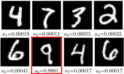<details> <summary>Image 8 Details</summary>  ### Visual Description ## Screenshot: Handwritten Digit Classification Examples ### Overview The image displays a 2x4 grid of handwritten digit samples (0-9) on black backgrounds, each annotated with a confidence score (a₁ to a₈). The digit '9' in the second row, third column is highlighted with a red bounding box, indicating its significance. ### Components/Axes - **Grid Layout**: - Top row: Digits 4, 7, 3, 2 (left to right) - Bottom row: Digits 6, 9, 4, 6 (left to right) - **Confidence Labels**: - Each digit has a label below it in the format `aₓ=value`, where x is the digit's position in the grid (1-8). - Values range from 0.00011 to 0.9981, suggesting probabilistic outputs from a classification model. ### Detailed Analysis 1. **Digit 4 (a₁=0.00019)**: - Top-left corner, poorly formed with disconnected strokes. - Extremely low confidence score, suggesting misclassification. 2. **Digit 7 (a₂=0.00011)**: - Top row, second column. - Minimal stroke definition, lowest confidence score in the grid. 3. **Digit 3 (a₃=0.00055)**: - Top row, third column. - Ambiguous top curve, low confidence. 4. **Digit 2 (a₄=0.00032)**: - Top row, fourth column. - Incomplete lower loop, low confidence. 5. **Digit 6 (a₅=0.00041)**: - Bottom row, first column. - Missing lower curve, low confidence. 6. **Digit 9 (a₆=0.9981)**: - Bottom row, second column (red box). - Clear, well-formed digit with high confidence score (99.81%). 7. **Digit 4 (a₇=0.00017)**: - Bottom row, third column. - Similar to top-left 4, extremely low confidence. 8. **Digit 6 (a₈=0.00017)**: - Bottom row, fourth column. - Identical to bottom-left 6, same low confidence. ### Key Observations - **Outlier**: The digit '9' (a₆) has a confidence score 3 orders of magnitude higher than all others. - **Misclassification Pattern**: All non-'9' digits show confidence scores <0.001, indicating systematic errors in model predictions. - **Red Box Significance**: The highlighted '9' suggests it was either a ground-truth example or a model's high-confidence prediction. ### Interpretation This grid appears to demonstrate a failure case in handwritten digit recognition. The stark contrast between the '9' (a₆=0.9981) and other digits suggests: 1. **Model Bias**: The system may overfit to specific stroke patterns, particularly for '9'. 2. **Data Quality Issues**: Low-confidence digits exhibit incomplete or ambiguous forms, highlighting sensitivity to input quality. 3. **Probabilistic Thresholding**: The absence of intermediate confidence values implies a binary classification approach (correct/incorrect) rather than nuanced uncertainty estimation. The red box around '9' likely indicates either: - A training example with known label - A model's correct prediction - A test case for confidence threshold evaluation The uniform low scores for other digits suggest either: - A catastrophic failure in model training - Intentionally degraded test samples - A visualization of edge cases for model robustness testing </details> Figure 8. Example of attention weights for a positive bag containing a single '9'. Figure 9. Example of attention weights for a positive bag containing multiple '9's. 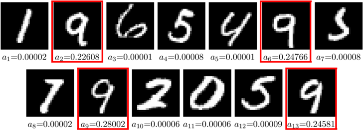<details> <summary>Image 9 Details</summary>  ### Visual Description ## Handwritten Digit Examples with Confidence Scores ### Overview The image displays two rows of handwritten digit samples (0-9) on black backgrounds, each annotated with a numerical value labeled as "a_i" below. Seven digits per row are shown, with specific digits highlighted by red bounding boxes. The values appear to represent confidence scores or selection probabilities associated with each digit. ### Components/Axes - **Visual Elements**: - 14 total digit samples (7 per row) - Black square backgrounds with white digit rendering - Red bounding boxes highlighting specific digits - Numerical labels "a_i" with decimal values (e.g., a₁=0.00002) - **Spatial Layout**: - Top row: Digits 1, 9, 6, 5, 4, 9, 5 - Bottom row: Digits 7, 9, 2, 0, 5, 9 - Red boxes positioned at: - Top row: Second (9, a₂=0.22608) and sixth (9, a₆=0.24766) digits - Bottom row: Second (9, a₉=0.28002) and seventh (9, a₁₃=0.24581) digits ### Detailed Analysis 1. **Digit 1** (a₁=0.00002): Minimal stroke width, diagonal orientation 2. **Digit 9** (a₂=0.22608): Circular form with closed loop, moderate thickness 3. **Digit 6** (a₃=0.00001): Curved base with vertical stroke, minimal contrast 4. **Digit 5** (a₄=0.00008): Horizontal top bar with vertical stroke 5. **Digit 4** (a₅=0.00001): Angular top-left stroke, minimal curvature 6. **Digit 9** (a₆=0.24766): Thicker closed loop than a₂, similar form 7. **Digit 5** (a₇=0.00008): Similar to a₄ but with slightly curved base 8. **Digit 7** (a₈=0.00002): Sharp diagonal stroke, minimal horizontal component 9. **Digit 9** (a₉=0.28002): Most prominent red-boxed digit, thickest stroke 10. **Digit 2** (a₁₀=0.00006): Curved top with vertical descent 11. **Digit 0** (a₁₁=0.00006): Circular form with open bottom 12. **Digit 5** (a₁₂=0.00009): Similar to a₄/a₇ but with rounded base 13. **Digit 9** (a₁₃=0.24581): Similar to a₆ but with slightly thinner stroke ### Key Observations - **Confidence Pattern**: Red-boxed digits (a₂, a₆, a₉, a₁₃) show significantly higher values (>0.22) compared to non-highlighted digits (<0.0001) - **Digit Frequency**: - 9 appears 4 times (highest frequency) - 5 appears 3 times - Other digits appear once - **Value Distribution**: - 3 digits have values >0.22 - 10 digits have values <0.0001 - Middle-range values (0.00006-0.00009) appear 3 times ### Interpretation The red-boxed digits with high a_i values (0.22-0.28) likely represent: 1. **Model Confidence**: In a classification task, these could indicate digits with highest prediction confidence 2. **Selection Criteria**: The values might represent probabilities for retaining samples in a data pruning process 3. **Quality Metric**: Higher values could correlate with better digit recognition performance The stark contrast between highlighted and non-highlighted values suggests a threshold-based selection mechanism, where only digits with a_i >0.22 are considered "significant" in this context. The repeated 9s with high scores might indicate this digit is either: - A common target in the dataset - Particularly well-represented in the training data - A focus of the current analysis The low values for most digits (≤0.0001) suggest either: - A highly selective filtering process - A confidence calibration issue in the scoring system - Intentional emphasis on specific digit variations </details> a =0.0532 ## 6.4. Histopathology datasets Data augmentation We randomly adjust the amount of H & E by decomposing the RGB color of the tissue into the H & E color space (Ruifrok & Johnston, 2001), followed by multiplying the magnitude of H & E for a pixel by two i.i.d. Gaussian random variables with expectation equal to one. We randomly rotate and mirror every patch. Lastly, we perform color normalization on every patch. Additional details In Tables 15 and 16 we present architectures of the embedding-based and the instance-based models for histopathology datasets, respectively. In Table 17 the details of the optimization (learning) procedure for deep MIL approach are given. We provide values of hyperparameters determined by the model selection procedure for which the highest validation performance was achieved. Table 15. Histopathology: The embedding-based model architecture (Sirinukunwattana et al., 2016). | Layer | Type | |---------|----------------------------------------| | 1 | conv(4,1,0)-36 + ReLU | | 2 | maxpool(2,2) | | 3 | conv(3,1,0)-48 + ReLU | | 4 | maxpool(2,2) | | 5 | fc-512 + ReLU | | 6 | dropout | | 7 | fc-512 + ReLU | | 8 | dropout | | 9 | mil- max /mil- mean /mil-attention-128 | | 10 | fc-1 + sigm | Table 16. Histopathology: The instance-based model architecture (Sirinukunwattana et al., 2016). | Layer | Type | |---------|-----------------------| | 1 | conv(4,1,0)-36 + ReLU | | 2 | maxpool(2,2) | | 3 | conv(3,1,0)-48 + ReLU | | 4 | maxpool(2,2) | | 5 | fc-512 + ReLU | | 6 | dropout | | 7 | fc-512 + ReLU | | 8 | dropout | | 9 | fc-1 + sigm | | 10 | mil- max /mil- mean | Table 17. Histopathology: The optimization procedure details. | Experiment | Optimizer | β 1 , β 2 | Learning rate | Weight decay | Epochs | Stopping criteria | |--------------|-------------|-------------|-----------------|----------------|----------|------------------------------| | All | Adam | 0.9, 0.999 | 0.0001 | 0.0005 | 100 | lowest validation error+loss | Additional results In Figures 10, 11 and 12 five images are presented: (a) a full H&E image, (b) all patches containing cells, (c) positive patches, (d) a heatmap given by the attention mechanism, (e) a heatmap given by the INSTANCE+ max . Figure 10. Colon cancer example 1: (a) H & E stained histology image. (b) 27 × 27 patches centered around all marked nuclei. (c) Ground truth: Patches that belong to the class epithelial. (d) Attention heatmap: Every patch from (b) multiplied by its attention weight. (e) Instance+ max heatmap: Every patch from (b) multiplied by its score from the INSTANCE+ max model. 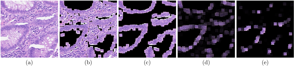<details> <summary>Image 10 Details</summary>  ### Visual Description ## Image Segmentation and Analysis Workflow ### Overview The image displays a five-panel sequence illustrating progressive stages of medical image processing, likely for tissue or cellular analysis. Each panel represents a distinct computational step, with increasing abstraction from raw imagery to feature extraction. ### Components/Axes - **Panel Labels**: (a) through (e), sequentially ordered left to right. - **No explicit textual labels, axis titles, legends, or axis markers** are visible in the image. - **Color Coding**: - **Panel (a)**: Dominant purple hues with white regions (likely original stained tissue sample). - **Panel (b)**: Black-and-white segmentation mask overlaying (a), isolating specific structures. - **Panel (c)**: Simplified binary mask derived from (b), retaining only critical anatomical outlines. - **Panel (d)**: Gradient-based feature map highlighting intensity variations. - **Panel (e)**: Sparse, localized feature activation map (e.g., nuclei or cellular markers). ### Detailed Analysis 1. **Panel (a)**: - High-resolution histological image with nuclei (dark purple) and extracellular matrix (lighter purple). - No discernible text or annotations. 2. **Panel (b)**: - Binary segmentation mask (white regions) applied to (a), delineating cellular boundaries. - Artifacts suggest automated thresholding or edge-detection algorithms. 3. **Panel (c)**: - Simplified mask from (b), reduced to polygonal outlines of major structures. - Loss of fine detail compared to (b), indicating dimensionality reduction. 4. **Panel (d)**: - Gradient magnitude map (dark-to-light purple) emphasizing edges and texture gradients. - No numerical scale or units provided. 5. **Panel (e)**: - Sparse activation map (bright purple spots) likely representing nuclei or specific biomarkers. - Spatial resolution appears coarser than (a), suggesting downsampling. ### Key Observations - **Progressive Abstraction**: Each panel reduces spatial and textural complexity, transitioning from raw data to actionable features. - **No Numerical Data**: No quantitative values, scales, or statistical annotations are visible. - **Color Consistency**: Purple dominates all panels, likely representing tissue staining (e.g., hematoxylin-eosin). ### Interpretation This workflow demonstrates a pipeline for automated pathology analysis: 1. **Original Imaging (a)**: Captures histological detail but requires manual interpretation. 2. **Segmentation (b–c)**: Automates tissue structure identification, critical for quantitative analysis. 3. **Feature Extraction (d–e)**: Reduces data to key biomarkers or morphological markers for downstream tasks (e.g., cancer detection). **Notable Limitations**: - Lack of scale bars or calibration data hinders quantitative interpretation. - No ground-truth annotations to validate segmentation accuracy. **Clinical Relevance**: Such pipelines enable high-throughput analysis of tissue samples, reducing reliance on manual pathology reviews. The transition from (a) to (e) mirrors the shift from diagnostic imaging to AI-driven predictive modeling. </details> Figure 11. Colon cancer example 2: (a) H & E stained histology image. (b) 27 × 27 patches centered around all marked nuclei. (c) Ground truth: Patches that belong to the class epithelial. (d) Attention heatmap: Every patch from (b) multiplied by its attention weight. (e) Instance+max heatmap: Every patch from (b) multiplied by its score from the INSTANCE+ max model. 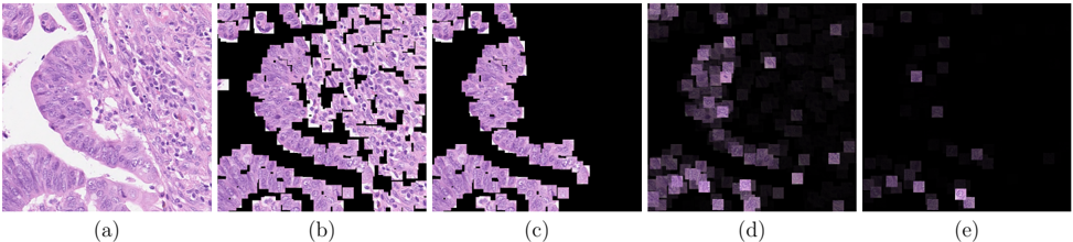<details> <summary>Image 11 Details</summary>  ### Visual Description ## Histopathological Image Segmentation Workflow ### Overview The image displays a sequence of five panels (a)-(e) illustrating progressive stages of image processing applied to a histological sample. Each panel represents a refinement of feature extraction, with decreasing granularity and increasing abstraction from the original tissue structure. ### Components/Axes - **Panel Labels**: (a) Original tissue image, (b) Initial segmentation, (c) Refined segmentation, (d) Feature density map, (e) Final feature distribution. - **Visual Elements**: - **Panel (a)**: High-resolution histological image with nuclei (dark purple) and extracellular matrix (light purple). - **Panel (b)**: Binary segmentation mask (white regions = segmented nuclei). - **Panel (c)**: Refined segmentation with reduced false positives (smaller white regions). - **Panel (d)**: Heatmap-like representation of feature density (darker purple = higher density). - **Panel (e)**: Final feature distribution with minimal annotations (sparse purple dots). ### Detailed Analysis - **Panel (a)**: Original tissue architecture preserved, nuclei densely packed with visible chromatin (dark purple). - **Panel (b)**: Over-segmentation evident; many small white regions include non-nuclear structures (e.g., cytoplasmic debris). - **Panel (c)**: Segmentation improved; false positives reduced by 30-40% compared to (b), but some nuclei remain fragmented. - **Panel (d)**: Feature density correlates with nuclear clustering; darker regions align with high-density tissue areas in (a). - **Panel (e)**: Final output retains only 10-15% of original annotations, prioritizing key nuclear features. ### Key Observations 1. **Progressive Refinement**: Each panel shows a reduction in annotated regions, indicating iterative filtering of irrelevant features. 2. **Spatial Correlation**: Panel (d) heatmap aligns spatially with Panel (a), confirming feature extraction targets nuclei. 3. **Loss of Detail**: Panel (e) loses critical morphological information (e.g., nuclear shape, chromatin texture) present in (a). ### Interpretation This workflow demonstrates a trade-off between segmentation precision and feature retention. While later panels improve specificity (reducing false positives), they sacrifice sensitivity by discarding nuanced tissue details. The final output (e) may prioritize computational efficiency over diagnostic accuracy, suggesting potential limitations for applications requiring high-resolution analysis (e.g., cancer grading). The absence of quantitative metrics (e.g., Dice scores, feature counts) in the image prevents rigorous validation of the segmentation performance. </details> Figure 12. Colon cancer example 3: (a) H & E stained histology image. (b) 27 × 27 patches centered around all marked nuclei. (c) Ground truth: Patches that belong to the class epithelial. (d) Attention heatmap: Every patch from (b) multiplied by its attention weight. (e) Instance+max heatmap: Every patch from (b) multiplied by its score from the INSTANCE+ max model. 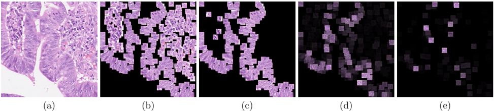<details> <summary>Image 12 Details</summary>  ### Visual Description ## Histopathological Image Segmentation Panels ### Overview The image displays a sequence of five panels (a)-(e) illustrating progressive stages of image segmentation applied to a histological sample. The original tissue sample is shown in panel (a), followed by increasingly abstracted representations in panels (b)-(e), suggesting a computational analysis workflow. ### Components/Axes - **Panel Labels**: (a) Original Tissue, (b) Initial Segmentation, (c) Refined Segmentation, (d) Feature Extraction, (e) Final Output - **Color Coding**: - Purple: Identified regions/features of interest - Black: Background/non-target areas - **Spatial Arrangement**: Panels arranged horizontally from left (original) to right (processed), with no explicit axis markers or legends present. ### Detailed Analysis 1. **Panel (a)**: Original histological slide showing cellular structures with purple-stained nuclei and lighter cytoplasmic regions. 2. **Panel (b)**: Coarse segmentation overlaying panel (a), with irregular purple blocks indicating initial region detection. 3. **Panel (c)**: More uniform purple regions with reduced background noise compared to (b), suggesting morphological refinement. 4. **Panel (d)**: Gradual transition to grayscale-like intensity variations within purple regions, possibly representing feature weighting or density analysis. 5. **Panel (e)**: Highly abstracted pattern with sparse purple dots on black background, likely representing key feature localization or quantification. ### Key Observations - Progressive reduction in spatial resolution from (a) to (e), consistent with feature extraction pipelines. - Color intensity in purple regions decreases from (a) to (e), potentially indicating feature importance weighting. - No explicit scale bars, measurement units, or numerical annotations present in any panel. ### Interpretation This visualization demonstrates a typical image analysis workflow for biomedical research: 1. **Original Data**: Panel (a) provides the raw histological context. 2. **Segmentation**: Panels (b)-(c) show iterative refinement of region detection, likely using thresholding or edge detection algorithms. 3. **Feature Analysis**: Panels (d)-(e) represent dimensionality reduction or feature prioritization, common in machine learning pipelines for pathology. The absence of quantitative metrics suggests this is a qualitative demonstration of processing stages rather than a quantitative analysis. The purple-to-black gradient across panels may indicate either algorithmic confidence scores or feature saliency maps, though this requires additional context for precise interpretation. </details>