1811.02440

## Gradual Type Theory(Extended Version) MAX S. NEW, Northeastern University DANIEL R. LICATA, Wesleyan University AMAL AHMED, Northeastern University and Inria Paris Gradually typed languages are designed to support both dynamically typed and statically typed programming styles while preserving the benefits of each. While existing gradual type soundness theorems for these languages aim to show that type-based reasoning is preserved when moving from the fully static setting to a gradual one, these theorems do not imply that correctness of type-based refactorings and optimizations is preserved. Establishing correctness of program transformations is technically difficult, because it requires reasoning about program equivalence, and is often neglected in the metatheory of gradual languages. In this paper, we propose an axiomatic account of program equivalence in a gradual cast calculus, which we formalize in a logic we call gradual type theory (GTT). Based on Levy's call-by-push-value, GTT gives an axiomatic account of both call-by-value and call-by-name gradual languages. Based on our axiomatic account we prove many theorems that justify optimizations and refactorings in gradually typed languages. For example, uniqueness principles for gradual type connectives show that if the βη laws hold for a connective, then casts between that connective must be equivalent to the so-called 'lazy' cast semantics. Contrapositively, this shows that 'eager' cast semantics violates the extensionality of function types. As another example, we show that gradual upcasts are pure functions and, dually, gradual downcasts are strict functions. We show the consistency and applicability of our axiomatic theory by proving that a contract-based implementation using the lazy cast semantics gives a logical relations model of our type theory, where equivalence in GTT implies contextual equivalence of the programs. Since GTT also axiomatizes the dynamic gradual guarantee, our model also establishes this central theorem of gradual typing. The model is parametrized by the implementation of the dynamic types, and so gives a family of implementations that validate type-based optimization and the gradual guarantee. CCS Concepts: · Theory of computation → Axiomatic semantics ; · Software and its engineering → Functional languages ; Additional Key Words and Phrases: gradual typing, graduality, call-by-push-value ## 1 INTRODUCTION Gradually typed languages are designed to support a mix of dynamically typed and statically typed programmingstyles and preserve the benefits of each. Dynamically typed code can be written without conforming to a syntactic type discipline, so the programmer can always run their program interactively with minimal work. On the other hand, statically typed code provides mathematically sound reasoning principles that justify type-based refactorings, enable compiler optimizations, and underlie formal software verification. The difficulty is accommodating both of these styles and their benefits simultaneously: allowing the dynamic and static code to interact without forcing the dynamic code to be statically checked or violating the correctness of type-based reasoning. The linchpin to the design of a gradually typed language is the semantics of runtime type casts . These are runtime checks that ensure that typed reasoning principles are valid by checking types of dynamically typed code at the boundary between static and dynamic typing. For instance, when a statically typed function f : Num → Num is applied to a dynamically typed argument x : ?, the language runtime must check if x is a number, and otherwise raise a dynamic type error. A programmer familiar with dynamically typed programming might object that this is overly strong: for Authors' addresses: Max S. New, Northeastern University, maxnew@ccs.neu.edu; Daniel R. Licata, Wesleyan University, dlicata@wesleyan.edu; Amal Ahmed, Northeastern University and Inria Paris, amal@ccs.neu.edu. instance if f is just a constant function f = λx : Num . 0 then why bother checking if x is a number since the body of the program does not seem to depend on it? The reason the value is rejected is because the annotation x : Num should introduce an assumption that that the programmer, compiler and automated tools can rely on for behavioral reasoning in the body of the function. For instance, if the variable x is guaranteed to only be instantiated with numbers, then the programmer is free to replace 0 with x -x or vice-versa. However, if x can be instantiated with a closure, then x -x will raise a runtime type error while 0 will succeed, violating the programmers intuition about the correctness of refactorings. We can formalize such relationships by observational equivalence of programs: the two closures λx : Num . 0 and λx : Num . x -x are indistinguishable to any other program in the language. This is precisely the difference between gradual typing and so-called optional typing: in an optionally typed language (Hack, TypeScript, Flow), annotations are checked for consistency but are unreliable to the user, so provide no leverage for reasoning. In a gradually typed language, type annotations should relieve the programmer of the burden of reasoning about incorrect inputs, as long as we are willing to accept that the program as a whole may crash, which is already a possibility in many effectful statically typed languages. However, the dichotomy between gradual and optional typing is not as firm as one might like. There have been many different proposed semantics of run-time type checking: 'transient' cast semantics [Vitousek et al. 2017] only checks the head connective of a type (number, function, list, . . . ), 'eager' cast semantics [Herman et al. 2010] checks run-time type information on closures, whereas 'lazy' cast semantics [Findler and Felleisen 2002] will always delay a type-check on a function until it is called (and there are other possibilities, see e.g. [Siek et al. 2009; Greenberg 2015]). The extent to which these different semantics have been shown to validate type-based reasoning has been limited to syntactic type soundness and blame soundness theorems. In their strongest form, these theorems say 'If t is a closed program of type A then it diverges, or reduces to a runtime error blaming dynamically typed code, or reduces to a value that satisfies A to a certain extent.' However, the theorem at this level of generality is quite weak, and justifies almost no program equivalences without more information. Saying that a resulting value satisfies type A might be a strong statement, but in transient semantics constrains only the head connective. The blame soundness theorem might also be quite strong, but depends on the definition of blame, which is part of the operational semantics of the language being defined. We argue that these type soundness theorems are only indirectly expressing the actual desired properties of the gradual language, which are program equivalences in the typed portion of the code that are not valid in the dynamically typed portion. Such program equivalences typically include β -like principles, which arise from computation steps, as well as η equalities , which express the uniqueness or universality of certain constructions. The η law of the untyped λ -calculus, which states that any λ -term M ≡ λx . Mx , is restricted in a typed language to only hold for terms of function type M : A → B ( λ is the unique/universal way of making an element of the function type). This famously 'fails' to hold in call-by-value languages in the presence of effects: if M is a program that prints "hello" before returning a function, then M will print now , whereas λx . Mx will only print when given an argument. But this can be accommodated with one further modification: the η law is valid in simple call-by-value languages 1 (e.g. SML) if we have a 'value restriction' V ≡ λx . Vx . This illustrates that η /extensionality rules must be stated for each type connective, and be sensitive to the effects/evaluation order of the terms involved. For instance, the η principle for the boolean type Bool in call-by-value is that for any term M with a free variable x : Bool , M is equivalent to a term that performs an if statement on 1 This does not hold in languages with some intensional feature of functions such as reference equality. We discuss the applicability of our main results more generally in Section 7. x : M ≡ if x ( M [ true / x ])( M [ false / x ]) . If we have an if form that is strongly typed (i.e., errors on non-booleans) then this tells us that it is safe to run an if statement on any input of boolean type (in CBN, by contrast an if statement forces a thunk and so is not necessarily safe). In addition, even if our if statement does some kind of coercion, this tells us that the term M only cares about whether x is 'truthy' or 'falsy' and so a client is free to change e.g. one truthy value to a different one without changing behavior. This η principle justifies a number of program optimizations, such as dead-code and common subexpression elimination, and hoisting an if statement outside of the body of a function if it is well-scoped ( λx . if y M N ≡ if y ( λx . M ) ( λx . N ) ). Any eager datatype, one whose elimination form is given by pattern matching such as 0 , + , 1 , × , list , has a similar η principle which enables similar reasoning, such as proofs by induction. The η principles for lazy types in call-by-name support dual behavioral reasoning about lazy functions, records, and streams. An Axiomatic Approach to Gradual Typing. In this paper, we systematically study questions of program equivalence for a class of gradually typed languages by working in an axiomatic theory of gradual program equivalence, a language and logic we call gradual type theory (GTT). Gradual type theory is the combination of a language of terms and gradual types with a simple logic for proving program equivalence and error approximation (equivalence up to one program erroring whenthe other does not) results. The logic axiomatizes the equational properties gradual programs should satisfy, and offers a high-level syntax for proving theorems about many languages at once: if a language models gradual type theory, then it satisfies all provable equivalences/approximations. Due to its type-theoretic design, different axioms of program equivalence are easily added or removed. Gradual type theory can be used both to explore language design questions and to verify behavioral properties of specific programs, such as correctness of optimizations and refactorings. To get off the ground, we take two properties of the gradual language for granted. First, we assume a compositionality property: that any cast from A to B can be factored through the dynamic type ?, i.e., the cast 〈 B ⇐ A 〉 t is equivalent to first casting up from A to ? and then down to B : 〈 B ⇐ ? 〉〈 ? ⇐ A 〉 t . These casts often have quite different performance characteristics, but should have the same extensional behavior: of the cast semantics presented in Siek et al. [2009], only the partially eager detection strategy violates this principle, and this strategy is not common. The second property we take for granted is that the language satisfies the dynamic gradual guarantee [Siek et al. 2015a] ('graduality')-a strong correctness theorem of gradual typing- which constrains how changing type annotations changes behavior. Graduality says that if we change the types in a program to be 'more precise'-e.g., by changing from the dynamic type to a more precise type such as integers or functions-the program will either produce the same behavior as the original or raise a dynamic type error. Conversely, if a program does not error and some types are made 'less precise' then behavior does not change. Wethen study what program equivalences are provable in GTT under various assumptions. Our central application is to study when the β , η equalities are satisfied in a gradually typed language. We approach this problem by a surprising tack: rather than defining the behavior of dynamic type casts and then verifying or invalidating the β and η equalities, we assume the language satisfies β and η equality and then show that certain reductions of casts are in fact program equivalence theorems deducible from the axioms of GTT. The cast reductions that we show satisfy all three constraints are those given by the 'lazy cast semantics' [Findler and Felleisen 2002; Siek et al. 2009]. As a contrapositive, any gradually typed language for which these reductions are not program equivalences is not a model of the axioms of gradual type theory. This mean the language violates either compositionality, the gradual guarantee, or one of the β , η axioms-and in practice, it is usually η . For instance, a transient semantics, where only the top-level connectives are checked, violates η for strict pairs <!-- formula-not-decoded --> because the top-level connectives of A 1 and A 2 are only checked when the pattern match is introduced. As a concrete counterexample to contextual equivalence, let A 1 , A 2 all be String . Because only the top-level connective is checked, ( 0 , 1 ) is a valid value of type String × String , but pattern matching on the pair ensures that the two components are checked to be strings, so the left-hand side let ( x 1 , x 2 ) = ( 0 , 1 ) ; 0 ↦→ /Omegainv (raises a type error). On the right-hand side, with no pattern, match a value (0) is returned. This means simple program changes that are valid in a typed language, such as changing a function of two arguments to take a single pair of those arguments, are invalidated by the transient semantics. In summary, transient semantics is 'lazier' than the types dictate, catching errors only when the term is inspected. As a subtler example, in call-by-value 'eager cast semantics' the βη principles for all of the eager datatypes (0 , + , 1 , × , lists, etc.) will be satisfied, but the η principle for the function type → is violated: there are values V : A → A ′ for which V /nequal λx : A . Vx . For instance, take an arbitrary function value V : A → String for some type A , and let V ′ = 〈 A → ? ⇐ A → String 〉 V be the result of casting it to have a dynamically typed output. Then in eager semantics, the following programs are not equivalent: <!-- formula-not-decoded --> We cannot observe any difference between these two programs by applying them to arguments, however, they are distinguished from each other by their behavior when cast . Specifically, if we cast both sides to A → Number , then 〈 A → Number ⇐ A → ? 〉( λx : A . V ′ x ) is a value, but 〈 A → Number ⇐ A → ? 〉 V ′ reduces to an error because Number is incompatible with String . However this type error might not correspond to any actual typing violation of the program involved. For one thing, the resulting function might never be executed. Furthermore, in the presence of effects, it may be that the original function V : A → String never returns a string (because it diverges, raises an exception or invokes a continuation), and so that same value casted to A → Number might be a perfectly valid inhabitant of that type. In summary the 'eager' cast semantics is in fact overly eager: in its effort to find bugs faster than 'lazy' semantics it disables the very type-based reasoning that gradual typing should provide. While criticisms of transient semantics on the basis of type soundness have been made before [Greenman and Felleisen 2018], our development shows that the η principles of types are enough to uniquely determine a cast semantics, and helps clarify the trade-off between eager and lazy semantics of function casts. Technical Overview of GTT. The gradual type theory developed in this paper unifies our previous work on operational (logical relations) reasoning for gradual typing in a call-by-value setting [New and Ahmed 2018] (which did not consider a proof theory), and on an axiomatic proof theory for gradual typing [New and Licata 2018] in a call-by-name setting (which considered only function and product types, and denotational but not operational models). In this paper, we develop an axiomatic gradual type theory GTT for a unified language that includes both call-by-value/eager types and call-by-name/lazy types (Sections 2, 3), and show that it is sound for contextual equivalence via a logical relations model (Sections 4, 5, 6). Because the η principles for types play a key role in our approach, it is necessary to work in a setting where we can have η principles for both eager and lazy types. We use Levy's Call-by-Push-Value [Levy 2003] (CBPV), which fully and faithfully embeds both call-by-value and call-by-name evaluation with both eager and lazy datatypes, 2 and underlies much recent work on reasoning about effectful 2 The distinction between 'lazy' vs 'eager' casts above is different than lazy vs. eager datatypes. programs [Bauer and Pretnar 2013; Lindley et al. 2017]. GTT can prove results in and about existing call-by-value gradually typed languages, and also suggests a design for call-by-name and full call-by-push-value gradually typed languages. In the prior work [New and Licata 2018; New and Ahmed 2018], gradual type casts are decomposed into upcasts and downcasts, as suggested above. A type dynamism relation (corresponding to type precision [Siek et al. 2015a] and naïve subtyping [Wadler and Findler 2009]) controls which casts exist: a type dynamism A /subsetsqequal A ′ induces an upcast from A to A ′ and a downcast from A ′ to A . Then, a term dynamism judgement is used for equational/approximational reasoning about programs. Term dynamism relates two terms whose types are related by type dynamism, and the upcasts and downcasts are each specified by certain term dynamism judgements holding. This specification axiomatizes only the properties of casts needed to ensure the graduality theorem, and not their precise behavior, so cast reductions can be proved from it , rather than stipulated in advance. The specification defines the casts 'uniquely up to equivalence', which means that any two implementations satisfying it are behaviorally equivalent. We generalize this axiomatic approach to call-by-push-value (Section 2), where there are both eager/value types and lazy/computation types. This is both a subtler question than it might at first seem, and has a surprisingly nice answer: we find that upcasts are naturally associated with eager/value types and downcasts with lazy/computation types, and that the modalities relating values and computations induce the downcasts for eager/value types and upcasts for lazy/computation types. Moreover, this analysis articulates an important behavioral property of casts that was proved operationally for call-by-value in [New and Ahmed 2018] but missed for call-by-name in [New and Licata 2018]: upcasts for eager types and downcasts for lazy types are both 'pure' in a suitable sense, which enables more refactorings and program optimizations. In particular, we show that these casts can be taken to be (and are essentially forced to be) 'complex values' and 'complex stacks' (respectively) in call-by-push-value, which corresponds to a behavioral property of thunkability and linearity [Munch-Maccagnoni 2014]. We argue in Section 7 that this property is related to blame soundness. Our gradual type theory naturally has two dynamic types, a dynamic eager/value type and a dynamic lazy/computation type, where the former can be thought of as a sum of all possible values, and the latter as a product of all possible behaviors. At the language design level, gradual type theory can be used to prove that, for a variety of eager/value and lazy/computation types, the 'lazy' semantics of casts is the unique implementation satisfying β , η and graduality (Section 3). These behavioral equivalences can then be used in reasoning about optimizations, refactorings, and correctness of specific programs. Contract-Based Models. To show the consistency of GTT as a theory, and to give a concrete operational interpretation of its axioms and rules, we provide a concrete model based on an operational semantics. The model is a contract interpretation of GTT in that the 'built-in' casts of GTT are translated to ordinary functions in a CBPV language that perform the necessary checks. To keep the proofs high-level, we break the proof into two steps. First (Sections 4, 5), we translate the axiomatic theory of GTT into an axiomatic theory of CBPV extended with recursive types and an uncatchable error, implementing casts by CBPV code that does contract checking. Then (Section 6) we give an operational semantics for the extended CBPV and define a step-indexed biorthogonal logical relation that interprets the ordering relation on terms as contextual error approximation, which underlies the definition of graduality as presented in [New and Ahmed 2018]. Combining these theorems gives an implementation of the term language of GTT in which β , η are observational equivalences and the dynamic gradual guarantee is satisfied. Due to the uniqueness theorems of GTT, the only part of this translation that is not predetermined is the definition of the dynamic types themselves and the casts between 'ground' types and the dynamic types. We use CBPV to explore the design space of possible implementations of the dynamic types, and give one that faithfully distinguishes all types of GTT, and another more Scheme-like implementation that implements sums and lazy pairs by tag bits. Both can be restricted to the CBV or CBN subsets of CBPV, but the unrestricted variant is actually more faithful to Scheme-like dynamically typed programming, because it accounts for variable-argument functions. Our modular proof architecture allows us to easily prove correctness of β , η and graduality for all of these interpretations. Contributions. The main contributions of the paper are as follows. - (1) We present Gradual Type Theory in Section 2, a simple axiomatic theory of gradual typing. The theory axiomatizes three simple assumptions about a gradual language: compositionality, graduality, and type-based reasoning in the form of η equivalences. - (2) We prove many theorems in the formal logic of Gradual Type Theory in Section 3. These include the unique implementation theorems for casts, which show that for each type connective of GTT, the η principle for the type ensures that the casts must implement the lazy contract semantics. Furthermore, we show that upcasts are always pure functions and dually that downcasts are always strict functions, as long as the base type casts are pure/strict. - (3) To substantiate that GTT is a reasonable axiomatic theory for gradual typing, we construct models of GTT in Sections 4, 5 and 6.3. This proceeds in two stages. First (Section 4), we use call-by-push-value as a typed metalanguage to construct several models of GTT using different recursive types to implement the dynamic types of GTT and interpret the casts as embedding-projection pairs. This extends standard translations of dynamic typing into static typing using type tags: the dynamic value type is constructed as a recursive sum of basic value types, but dually the dynamic computation type is constructed as a recursive product of basic computation types. This dynamic computation type naturally models stack-based implementations of variable-arity functions as used in the Scheme language. - (4) We then give an operational model of the term dynamism ordering as contextual error approximation in Sections 5 and 6.3. To construct this model, we extend previous work on logical relations for error approximation from call-by-value to call-by-push-value [New and Ahmed 2018], simplifying the presentation in the process. ## 2 AXIOMATIC GRADUAL TYPE THEORY In this section we introduce the syntax of Gradual Type Theory, an extension of Call-by-pushvalue [Levy 2003] to support the constructions of gradual typing. First we introduce call-by-pushvalue and then describe in turn the gradual typing features: dynamic types, casts, and the dynamism orderings on types and terms. 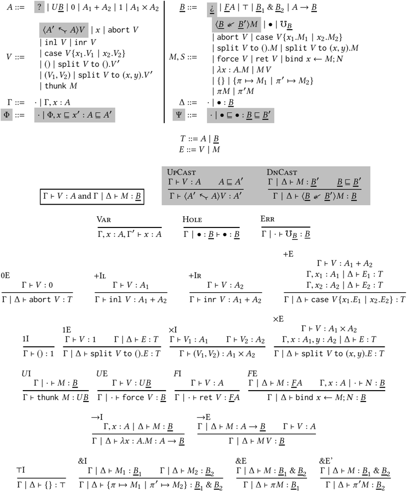## 2.1 Background: Call-by-Push-Value GTT is an extension of CBPV, so we first present CBPV as the unshaded rules in Figure 1. CBPV makes a distinction between value types A and computation types B , where value types classify values Γ /turnstileleft V : A and computation types classify computations Γ /turnstileleft M : B . Effects are computations: for example, we might have an error computation /Omegainv B : B of every computation type, or printing print V ; M : B if V : string and M : B , which prints V and then behaves as M . Value types and complex values. The value types include eager products 1 and A 1 × A 2 and sums 0 and A 1 + A 2, which behave as in a call-by-value/eager language (e.g. a pair is only a value when its components are). The notion of value V is more permissive than one might expect, and expressions Γ /turnstileleft V : A are sometimes called complex values to emphasize this point: complex values include not only closed runtime values, but also open values that have free value variables (e.g. x : A 1 , x 2 : A 2 /turnstileleft ( x 1 , x 2 ) : A 1 × A 2), and expressions that pattern-match on values (e.g. Fig. 1. GTT Syntax and Term Typing <details> <summary>Image 1 Details</summary>  ### Visual Description ## Type Theory Rules ### Overview The image presents a collection of type theory rules, defining the syntax and semantics of a formal system. It includes definitions for types, values, expressions, and typing judgments, along with inference rules for various language constructs. ### Components/Axes * **Top-Left**: Definitions for types `A`, values `V`. * **Top-Right**: Definitions for types `B`, expressions `M, S`. * **Middle-Left**: Definitions for contexts `Γ`, `Φ`. * **Middle-Right**: Definitions for contexts `Δ`, `Ψ`. * **Bottom**: Inference rules for type checking. ### Detailed Analysis or ### Content Details **Definitions:** * **Types (A)**: * `A ::= ? | UB | 0 | A1 + A2 | 1 | A1 X A2` * `?`: Unknown type. * `UB`: Unit type. * `0`: Empty type. * `A1 + A2`: Sum type. * `1`: Unit type. * `A1 X A2`: Product type. * **Values (V)**: * `V ::= <A' <- A> V | x | abort V | inl V | inr V | case V{x1.V1 | x2.V2} | () | split V to ().V' | (V1, V2) | split V to (x, y).V' | thunk M` * `<A' <- A> V`: Type cast. * `x`: Variable. * `abort V`: Abort. * `inl V`: Left injection. * `inr V`: Right injection. * `case V{x1.V1 | x2.V2}`: Case expression. * `()`: Unit value. * `split V to ().V'`: Split operation. * `(V1, V2)`: Pair. * `split V to (x, y).V'`: Split operation. * `thunk M`: Thunk. * **Types (B)**: * `B ::= ¿ | FA | T | B1 & B2 | A -> B` * `¿`: Unknown type. * `FA`: Type constructor. * `T`: Type variable. * `B1 & B2`: Product type. * `A -> B`: Function type. * **Expressions (M, S)**: * `M, S ::= <B <- B'> M | • | UB | abort V | case V{x1.M1 | x2.M2} | split V to ().M | split V to (x, y).M | force V | ret V | bind x <- M; N | λx: A.M | MV | {} | {π -> M1 | π' -> M2} | πM | π'M` * `<B <- B'> M`: Type cast. * `•`: Hole. * `UB`: Unit expression. * `abort V`: Abort. * `case V{x1.M1 | x2.M2}`: Case expression. * `split V to ().M`: Split operation. * `split V to (x, y).M`: Split operation. * `force V`: Force. * `ret V`: Return. * `bind x <- M; N`: Bind. * `λx: A.M`: Lambda abstraction. * `MV`: Application. * `{}`: Empty record. * `{π -> M1 | π' -> M2}`: Record. * `πM`: Projection. * `π'M`: Projection. * **Contexts (Γ)**: * `Γ ::= · | Γ, x: A` * `.`: Empty context. * `Γ, x: A`: Context extension. * **Contexts (Φ)**: * `Φ ::= · | Φ, x <- x': A ⊆ A'` * `.`: Empty context. * `Φ, x <- x': A ⊆ A'`: Context extension with subtyping. * **Contexts (Δ)**: * `Δ ::= · | • ⊆ B` * `.`: Empty context. * `• ⊆ B`: Context extension with subtyping. * **Contexts (Ψ)**: * `Ψ ::= · | • ⊆ B ⊆ B'` * `.`: Empty context. * `• ⊆ B ⊆ B'`: Context extension with subtyping. * **Other Definitions**: * `T ::= A | B` * `E ::= V | M` **Typing Rules:** * **Upcast**: * Premises: `Γ |- V: A`, `A ⊆ A'` * Conclusion: `Γ |- <A' <- A> V: A'` * **Downcast**: * Premises: `Γ |- Δ |- M: B'`, `B ⊆ B'` * Conclusion: `Γ |- Δ |- <B <- B'> M: B` * **Var**: * Conclusion: `Γ, x: A, Γ' |- x: A` * **Hole**: * Conclusion: `Γ |- •: B` * **Err**: * Conclusion: `Γ |- UB: B` * **0E**: * Premise: `Γ |- V: 0` * Conclusion: `Γ |- Δ |- abort V: T` * **+IL**: * Premise: `Γ |- V: A1` * Conclusion: `Γ |- inl V: A1 + A2` * **+IR**: * Premise: `Γ |- V: A2` * Conclusion: `Γ |- inr V: A1 + A2` * **+E**: * Premises: `Γ |- V: A1 + A2`, `Γ, x1: A1 |- Δ |- E1: T`, `Γ, x2: A2 |- Δ |- E2: T` * Conclusion: `Γ |- Δ |- case V{x1.E1 | x2.E2}: T` * **1I**: * Conclusion: `Γ |- (): 1` * **1E**: * Premise: `Γ |- V: 1` * Conclusion: `Γ |- Δ |- split V to ().E: T` * **xI**: * Premises: `Γ |- V1: A1`, `Γ |- V2: A2` * Conclusion: `Γ |- (V1, V2): A1 X A2` * **xE**: * Premises: `Γ |- V: A1 X A2`, `Γ, x: A1, y: A2 |- Δ |- E: T` * Conclusion: `Γ |- Δ |- split V to (x, y).E: T` * **UI**: * Premise: `Γ |- M: B` * Conclusion: `Γ |- thunk M: UB` * **UE**: * Premise: `Γ |- V: UB` * Conclusion: `Γ |- force V: B` * **FI**: * Premise: `Γ |- V: A` * Conclusion: `Γ |- ret V: FA` * **FE**: * Premises: `Γ |- Δ |- M: FA`, `Γ, x: A |- Δ |- N: B` * Conclusion: `Γ |- Δ |- bind x <- M; N: B` * **->I**: * Premise: `Γ, x: A |- Δ |- M: B` * Conclusion: `Γ |- Δ |- λx: A.M: A -> B` * **->E**: * Premises: `Γ |- Δ |- M: A -> B`, `Γ |- V: A` * Conclusion: `Γ |- Δ |- MV: B` * **TI**: * Conclusion: `Γ |- {}: T` * **&I**: * Premises: `Γ |- Δ |- M1: B1`, `Γ |- Δ |- M2: B2` * Conclusion: `Γ |- Δ |- {π -> M1 | π' -> M2}: B1 & B2` * **&E**: * Premise: `Γ |- Δ |- M: B1 & B2` * Conclusion: `Γ |- Δ |- πM: B1` * **&E'**: * Premise: `Γ |- Δ |- M: B1 & B2` * Conclusion: `Γ |- Δ |- π'M: B2` ### Key Observations * The system includes basic types like unit, empty, sum, and product. * It supports type casting, function abstraction and application, and record manipulation. * The typing rules define how to derive the type of an expression based on the types of its sub-expressions and the context. ### Interpretation The image presents a formal type system, likely for a functional programming language. The definitions and typing rules provide a rigorous framework for ensuring type safety and preventing runtime errors. The system includes features like subtyping, type casting, and record types, which enhance its expressiveness and flexibility. The rules are designed to be compositional, allowing the type of a complex expression to be derived from the types of its constituent parts. </details> p : A 1 × A 2 /turnstileleft split p to ( x 1 , x 2 ) . ( x 2 , x 1 ) : A 2 × A 1). Thus, the complex values x : A /turnstileleft V : A ′ are a syntactic class of 'pure functions' from A to A ′ (though there is no pure function type internalizing this judgement), which can be treated like values by a compiler because they have no effects (e.g. they can be dead-code-eliminated, common-subexpression-eliminated, and so on). In focusing [Andreoli 1992] terminology, complex values consist of left inversion and right focus rules.For each pattern-matching construct (e.g. case analysis on a sum, splitting a pair), we have both an elimination rule whose branches are values (e.g. split p to ( x 1 , x 2 ) . V ) and one whose branches are computations (e.g. split p to ( x 1 , x 2 ) . M ). To abbreviate the typing rules for both in Figure 1, weuse the following convention: we write E :: = V | M for either a complex value or a computation, and T :: = A | B for either a value type A or a computation type B , and a judgement Γ | ∆ /turnstileleft E : T for either Γ /turnstileleft V : A or Γ | ∆ /turnstileleft M : B (this is a bit of an abuse of notation because ∆ is not present in the former). Complex values can be translated away without loss of expressiveness by moving all pattern-matching into computations (see Section 5), at the expense of using a behavioral condition of thunkability [Munch-Maccagnoni 2014] to capture the properties complex values have (for example, an analogue of let x = V ; let x ′ = V ′ ; M ≡ let x ′ = V ′ ; let x = V ; M - complex values can be reordered, while arbitrary computations cannot). Shifts. A key notion in CBPV is the shift types FA and UB , which mediate between value and computation types: FA is the computation type of potentially effectful programs that return a value of type A , while UB is the value type of thunked computations of type B . The introduction rule for FA is returning a value of type A ( ret V), while the elimination rule is sequencing a computation M : FA with a computation x : A /turnstileleft N : B to produce a computation of a B ( bind x ← M ; N ). While any closed complex value V is equivalent to an actual value, a computation of type FA might perform effects (e.g. printing) before returning a value, or might error or non-terminate and not return a value at all. The introduction and elimination rules for U are written thunk M and force V , and say that computations of type B are bijective with values of type UB . As an example of the action of the shifts, 0 is the empty value type, so F 0 classifies effectful computations that never return, but may perform effects (and then, must e.g. non-terminate or error), while UF 0 is the value type where such computations are thunked/delayed and considered as values.1 is the trivial value type, so F 1 is the type of computations that can perform effects with the possibility of terminating successfully by returning () , and UF 1 is the value type where such computations are delayed values. UF is a monad on value types [Moggi 1991], while FU is a comonad on computation types. Computation types. The computation type constructors in CBPV include lazy unit/products /latticetop and B 1 & B 2 , which behave as in a call-by-name/lazy language (e.g. a component of a lazy pair is evaluated only when it is projected). Functions A → B have a value type as input and a computation type as a result. The equational theory of effects in CBPV computations may be surprising to those familiar only with call-by-value, because at higher computation types effects have a callby-name-like equational theory. For example, at computation type A → B , we have an equality print c ; λx . M = λx . print c ; M . Intuitively, the reason is that A → B is not treated as an observable type (one where computations are run): the states of the operational semantics are only those computations of type FA for some value type A . Thus, 'running' a function computation means supplying it with an argument, and applying both of the above to an argument V is defined to result in print c ; M [ V / x ] . This does not imply that the corresponding equations holds for the call-by-value function type, which we discuss below. As another example, all computations are considered equal at type /latticetop , even computations that perform different effects ( print c vs. {} vs. /Omegainv ), because there is by definition no way to extract an observable of type FA from a computation of type /latticetop . Consequently, U /latticetop is isomorphic to 1. Complex stacks. Just as the complex values V are a syntactic class terms that have no effects, CBPV includes a judgement for 'stacks' S , a syntactic class of terms that reflect all effects of their input. A stack Γ | · : B /turnstileleft S : B ′ can be thought of as a linear/strict function from B to B ′ , which must use its input hole · exactly once at the head redex position. Consequently, effects can be hoisted out of stacks, because we know the stack will run them exactly once and first. For example, there will be contextual equivalences S [ /Omegainv /·] = /Omegainv and S [ print V ; M ] = print V ; S [ M /·] . Just as complex values include pattern-matching, complex stacks include pattern-matching on values and introduction forms for the stack's output type. For example, · : B 1 & B 2 /turnstileleft { π ↦→ π ′ · | π ′ ↦→ π ·} : B 2 & B 1 is a complex stack, even though it mentions · more than once, because running it requires choosing a projection to get to an observable of type FA , so each time it is run it uses · exactly once. In focusing terms, complex stacks include both left and right inversion, and left focus rules.In the equational theory of CBPV, F and U are adjoint , in the sense that stacks · : FA /turnstileleft S : B are bijective with values x : A /turnstileleft V : UB , as both are bijective with computations x : A /turnstileleft M : B . To compress the presentation in Figure 1, we use a typing judgement Γ | ∆ /turnstileleft M : B with a 'stoup', a typing context ∆ that is either empty or contains exactly one assumption · : B , so Γ | · /turnstileleft M : B is a computation, while Γ | · : B /turnstileleft M : B ′ is a stack. The typing rules for /latticetop and & treat the stoup additively (it is arbitrary in the conclusion and the same in all premises); for a function application to be a stack, the stack input must occur in the function position. The elimination form for UB , force V , is the prototypical non-stack computation ( ∆ is required to be empty), because forcing a thunk does not use the stack's input. Embedding call-by-value and call-by-name. To translate call-by-value (CBV) into CBPV, a judgement x 1 : A 1 , . . . , x n : A n /turnstileleft e : A is interpreted as a computation x 1 : A v 1 , . . . , x n : A v n /turnstileleft e v : FA v , where call-by-value products and sums are interpreted as × and + , and the call-by-value function type A → A ′ as U ( A v → FA ′ v ) . Thus, a call-by-value term e : A → A ′ , which should mean an effectful computation of a function value, is translated to a computation e v : FU ( A v → FA ′ v ) . Here, the comonad FU offers an opportunity to perform effects before returning a function value-so under translation the CBV terms print c ; λx . e and λx . print c ; e will not be contextually equivalent. To translate call-by-name (CBN) to CBPV, a judgement x 1 : B 1 , . . . , x m : B m /turnstileleft e : B is translated to x 1 : UB 1 n , . . . , x m : UB m n /turnstileleft e n : B n , representing the fact that call-by-name terms are passed thunked arguments. Product types are translated to /latticetop and × , while a CBN function B → B ′ is translated to UB n → B ′ n with a thunked argument. Sums B 1 + B 2 are translated to F ( UB 1 n + UB 2 n ) , making the 'lifting' in lazy sums explicit. Call-by-push-value subsumes call-by-value and call-by-name in that these embeddings are full and faithful : two CBV or CBN programs are equivalent if and only if their embeddings into CBPV are equivalent, and every CBPV program with a CBV or CBN type can be back-translated. Extensionality/ η Principles. The main advantage of CBPV for our purposes is that it accounts for the η /extensionality principles of both eager/value and lazy/computation types, because value types have η principles relating them to the value assumptions in the context Γ , while computation types have η principles relating them to the result type of a computation B . For example, the η principle for sums says that any complex value or computation x : A 1 + A 2 /turnstileleft E : T is equivalent to case x { x 1 . E [ inl x 1 / x ] | x 2 . E [ inr x 2 / x ]} , i.e. a case on a value can be moved to any point in a program (where all variables are in scope) in an optimization. Given this, the above translations of CBV and CBN into CBPV explain why η for sums holds in CBV but not CBN: in CBV, x : A 1 + A 2 /turnstileleft E : T is translated to a term with x : A 1 + A 2 free, but in CBN, x : B 1 + B 2 /turnstileleft E : T is translated to a term with x : UF ( UB 1 + UB 2 ) free, and the type UF ( UB 1 + UB 2 ) of monadic computations that return a sum does not satisfy the η principle for sums in CBPV. Dually, the η principle for functions in CBPV is that any computation M : A → B is equal to λx . Mx . ACBNterm e : B → B ′ is translated to a CBPV computation of type UB → B ′ , to which CBPV function extensionality applies, while a CBV term e : A → A ′ is translated to a computation of type FU ( A → FA ′ ) , which does not satisfy the η rule for functions. We discuss a formal statement of these η principles with term dynamism below. ## 2.2 The Dynamic Type(s) Next, we discuss the additions that make CBPV into our gradual type theory GTT. A dynamic type plays a key role in gradual typing, and since GTT has two different kinds of types, we have a new question of whether the dynamic type should be a value type, or a computation type, or whether we should have both a dynamic value type and a dynamic computation type. Our modular, type-theoretic presentation of gradual typing allows us to easily explore these options, though we find that having both a dynamic value ? and a dynamic computation type ¿ gives the most natural implementation (see Section 4.2). Thus, we add both ? and ¿ to the grammar of types in Figure 1. We do not give introduction and elimination rules for the dynamic types, because we would like constructions in GTT to imply results for many different possible implementations of them. Instead, the terms for the dynamic types will arise from type dynamism and casts. ## 2.3 Type Dynamism The type dynamism relation of gradual type theory is written A /subsetsqequal A ′ and read as ' A is less dynamic than A ′ '; intuitively, this means that A ′ supports more behaviors than A . Our previous work [New and Ahmed 2018; New and Licata 2018] analyzes this as the existence of an upcast from A to A ′ and a downcast from A ′ to A which form an embedding-projection pair ( ep pair ) for term error approximation (an ordering where runtime errors are minimal): the upcast followed by the downcast is a no-op, while the downcast followed by the upcast might error more than the original term, because it imposes a run-time type check. Syntactically, type dynamism is defined (1) to be reflexive and transitive (a preorder), (2) where every type constructor is monotone in all positions, and (3) where the dynamic type is greatest in the type dynamism ordering. This last condition, the dynamic type is the most dynamic type , implies the existence of an upcast 〈 ? /arrowtailleft A 〉 and a downcast 〈 A /dblarrowheadleft ? 〉 for every type A : any type can be embedded into it and projected from it. However, this by design does not characterize ? uniquely-instead, it is open-ended exactly which types exist (so that we can always add more), and some properties of the casts are undetermined; we exploit this freedom in Section 4.2. This extends in a straightforward way to CBPV's distinction between value and computation types in Figure 2: there is a type dynamism relation for value types A /subsetsqequal A ′ and for computation types B /subsetsqequal B ′ , which (1) each are preorders (V TyRefl , VTyTrans , CTyRefl , CTyTrans ), (2) every type constructor is monotone ( + Mon , × Mon , & Mon , → Mon ) where the shifts F and U switch which relation is being considered ( U Mon , F Mon ), and (3) the dynamic types ? and ¿ are the most dynamic value and computation types respectively ( VTyTop , CTyTop ). For example, we have U ( A → FA ′ ) /subsetsqequal U ( ? → F ? ) , which is the analogue of A → A ′ /subsetsqequal ? → ? in call-byvalue: because → preserves embedding-retraction pairs, it is monotone, not contravariant, in the domain [New and Ahmed 2018; New and Licata 2018]. ## 2.4 Casts It is not immediately obvious how to add type casts to CPBV, because CBPV exposes finer judgemental distinctions than previous work considered. However, we can arrive at a first proposal by considering how previous work would be embedded into CBPV. In the previous work on both CBV and CBN [New and Ahmed 2018; New and Licata 2018] every type dynamism judgement A /subsetsqequal A ′ Fig. 2. GTT Type Dynamism and Dynamism Contexts | A /subsetsqequal A ′ and B /subsetsqequal B ′ | VTyRefl A /subsetsqequal A | VTyTrans A /subsetsqequal A ′ A ′ /subsetsqequal A ′′ A /subsetsqequal A ′′ | CTyRefl B /subsetsqequal B ′ | CTyTrans B /subsetsqequal B ′ B ′ /subsetsqequal B ′′ B /subsetsqequal B ′′ | |-------------------------------------------------|------------------------------|----------------------------------------------------------------------------------------------|--------------------------------|-------------------------------------------------------------------------------| | VTyTop | U Mon B /subsetsqequal B ′ | + Mon A 1 /subsetsqequal A ′ 1 A 2 /subsetsqequal A ′ 2 | × Mon A 1 /subsetsqequal A ′ 1 | A 2 /subsetsqequal A ′ 2 | | A /subsetsqequal ? | UB /subsetsqequal UB ′ | A 1 + A 2 /subsetsqequal A ′ 1 + A ′ 2 | A 1 × A 2 /subsetsqequal A | ′ 1 × A ′ 2 | | CTyTop | F Mon A /subsetsqequal A ′ | & Mon B 1 /subsetsqequal B ′ 1 B 2 /subsetsqequal B ′ 2 | → Mon A /subsetsqequal A ′ | B /subsetsqequal B ′ | | Dynamism contexts | · dyn - vctx | Φ dyn - vctx A /subsetsqequal A ′ Φ , x /subsetsqequal x ′ : A /subsetsqequal A ′ dyn - vctx | · dyn - cctx (• /subsetsqequal | B /subsetsqequal B • : B /subsetsqequal B ′ ) dyn - cctx | | | | | | ′ | induces both an upcast from A to A ′ and a downcast from A ′ to A . Because CBV types are associated to CBPV value types and CBN types are associated to CBPV computation types, this suggests that each value type dynamism A /subsetsqequal A ′ should induce an upcast and a downcast, and each computation type dynamism B /subsetsqequal B ′ should also induce an upcast and a downcast. In CBV, a cast from A to A ′ typically can be represented by a CBV function A → A ′ , whose analogue in CBPV is U ( A → FA ′ ) , and values of this type are bijective with computations x : A /turnstileleft M : FA ′ , and further with stacks · : FA /turnstileleft S : FA ′ . This suggests that a value type dynamism A /subsetsqequal A ′ should induce an embeddingprojection pair of stacks · : FA /turnstileleft S u : FA ′ and · : FA ′ /turnstileleft S d : FA , which allow both the upcast and downcast to a priori be effectful computations. Dually, a CBN cast typically can be represented by a CBN function of type B → B ′ , whose CBPV analogue is a computation of type UB → B ′ , which is equivalent with a computation x : UB /turnstileleft M : B ′ , and with a value x : UB /turnstileleft V : UB ′ . This suggests that a computation type dynamism B /subsetsqequal B ′ should induce an embedding-projection pair of values x : UB /turnstileleft V u : UB ′ and x : UB ′ /turnstileleft V d : UB , where both the upcast and the downcast again may a priori be (co)effectful, in the sense that they may not reflect all effects of their input. However, this analysis ignores an important property of CBV casts in practice: upcasts always terminate without performing any effects, and in some systems upcasts are even defined to be values, while only the downcasts are effectful (introduce errors). For example, for many types A , the upcast from A to ? is an injection into a sum/recursive type, which is a value constructor. Our previous work on a logical relation for call-by-value gradual typing [New and Ahmed 2018] proved that all upcasts were pure in this sense as a consequence of the embedding-projection pair properties (but their proof depended on the only effects being divergence and type error). In GTT, we can make this property explicit in the syntax of the casts, by making the upcast 〈 A ′ /arrowtailleft A 〉 induced by a value type dynamism A /subsetsqequal A ′ itself a complex value, rather than computation. On the other hand, many downcasts between value types are implemented as a case-analysis looking for a specific tag and erroring otherwise, and so are not complex values. We can also make a dual observation about CBN casts. The downcast arising from B /subsetsqequal B ′ has a stronger property than being a computation x : UB ′ /turnstileleft M : B as suggested above: it can be taken to be a stack · : B ′ /turnstileleft 〈 B /dblarrowheadleft B ′ 〉· : B , because a downcasted computation evaluates the computation it is 'wrapping' exactly once. One intuitive justification for this point of view, which we make precise in Section 4, is to think of the dynamic computation type ¿ as a recursive product of all possible behaviors that a computation might have, and the downcast as a recursive type unrolling Fig. 3. GTT Term Dynamism (Structural Rules) <details> <summary>Image 2 Details</summary>  ### Visual Description ## Type Theory Rules ### Overview The image presents a set of type theory rules, likely related to a dynamic semantics or type system. Each rule is formatted as an inference rule, with premises above a horizontal line and a conclusion below. The rules cover various aspects of type checking and evaluation, including reflexivity, variable lookup, transitivity, value substitution, hole filling, and stack substitution. ### Components/Axes The image contains six distinct inference rules, each labeled with a name starting with "TmDyn". The rules involve various type environments (Γ, Δ, Φ, Ψ), terms (E, V, M), types (T, A, B), and variables (x). The symbol "⊑" represents a subtyping or containment relation. ### Detailed Analysis **1. Top-Right Box:** * Text: "Φ ⊢ V ⊑ V': A ⊑ A' and Φ | Ψ ⊢ M ⊑ M': B ⊑ B'" * This appears to be a general condition or context applicable to some of the rules. It states that V is a subtype of V' with type A a subtype of A', and M is a subtype of M' with type B a subtype of B', all under contexts Φ and Ψ. **2. TmDynRefl (Top-Left):** * Rule: ``` Γ ⊑ Γ | Δ ⊑ Δ ⊢ E ⊑ E : T ⊑ T ``` * This rule states that if the type environment Γ is a subtype of itself, Δ is a subtype of itself, then E is a subtype of itself with type T a subtype of itself. This represents a reflexivity property. **3. TmDynVar (Top-Right):** * Rule: ``` Φ, x ⊑ x' : A ⊑ A', Φ' ⊢ x ⊑ x' : A ⊑ A' ``` * This rule states that if x is a subtype of x' with type A a subtype of A' in the context Φ, then x is a subtype of x' with type A a subtype of A' in the context Φ'. This represents variable lookup. **4. TmDynTrans (Middle-Left):** * Rule: ``` Γ ⊑ Γ' | Δ ⊑ Δ' ⊢ E ⊑ E' : T ⊑ T' Γ' ⊑ Γ'' | Δ' ⊑ Δ'' ⊢ E' ⊑ E'' : T' ⊑ T'' -------------------------------------------------- Γ ⊑ Γ'' | Δ ⊑ Δ'' ⊢ E ⊑ E'' : T ⊑ T'' ``` * This rule states that if Γ is a subtype of Γ', Δ is a subtype of Δ', and E is a subtype of E' with type T a subtype of T', and Γ' is a subtype of Γ'', Δ' is a subtype of Δ'', and E' is a subtype of E'' with type T' a subtype of T'', then Γ is a subtype of Γ'', Δ is a subtype of Δ'', and E is a subtype of E'' with type T a subtype of T''. This represents a transitivity property. **5. TmDynValSubst (Middle-Right):** * Rule: ``` Φ ⊢ V ⊑ V' : A ⊑ A' Φ, x ⊑ x' : A ⊑ A', Φ' | Ψ ⊢ E ⊑ E' : T ⊑ T' -------------------------------------------------- Φ | Ψ ⊢ E[V/x] ⊑ E'[V'/x'] : T ⊑ T' ``` * This rule states that if V is a subtype of V' with type A a subtype of A', and E is a subtype of E' with type T a subtype of T' in the context Φ, then E[V/x] is a subtype of E'[V'/x'] with type T a subtype of T' in the context Φ. This represents value substitution. **6. TmDynHole (Bottom-Left):** * Rule: ``` Φ | • ⊑ • : B ⊑ B' ⊢ • ⊑ • : B ⊑ B' ``` * This rule states that if the hole "•" is a subtype of itself with type B a subtype of B', then the hole "•" is a subtype of itself with type B a subtype of B'. This represents a hole filling. **7. TmDynStkSubst (Bottom-Right):** * Rule: ``` Φ | Ψ ⊢ M₁ ⊑ M₁' : B₁ ⊑ B₁' Φ | • ⊑ • : B₁ ⊑ B₁' ⊢ M₂ ⊑ M₂' : B₂ ⊑ B₂' -------------------------------------------------- Φ | Ψ ⊢ M₂[M₁/•] ⊑ M₂'[M₁'/•] : B₂ ⊑ B₂' ``` * This rule states that if M₁ is a subtype of M₁' with type B₁ a subtype of B₁', and M₂ is a subtype of M₂' with type B₂ a subtype of B₂', then M₂[M₁/•] is a subtype of M₂'[M₁'/•] with type B₂ a subtype of B₂'. This represents stack substitution. ### Key Observations * The rules define a subtyping relation between terms and types. * The rules are inference rules, meaning that the conclusion is valid if the premises are valid. * The rules cover various aspects of type checking and evaluation, including reflexivity, variable lookup, transitivity, value substitution, and stack substitution. ### Interpretation The rules likely define a dynamic semantics for a type system. The subtyping relation allows for flexibility in type checking, as a term of a subtype can be used where a term of a supertype is expected. The rules ensure that the subtyping relation is preserved during evaluation. The presence of rules for hole filling and stack substitution suggests that the type system may be used for program synthesis or interactive development. The rules are foundational for ensuring type safety and correctness in a programming language or system. </details> and product projection, which is a stack. From this point of view, an upcast can introduce errors, because the upcast of an object supporting some 'methods' to one with all possible methods will error dynamically on the unimplemented ones. These observations are expressed in the (shaded) UpCast and DnCasts rules for casts in Figure 1: the upcast for a value type dynamism is a complex value, while the downcast for a computation type dynamism is a stack (if its argument is). Indeed, this description of casts is simpler than the intuition we began the section with: rather than putting in both upcasts and downcasts for all value and computation type dynamisms, it suffices to put in only upcasts for value type dynamisms and downcasts for computation type dynamisms, because of monotonicity of type dynamism for U / F types. The downcast for a value type dynamism A /subsetsqequal A ′ , as a stack · : FA ′ /turnstileleft 〈 FA /dblarrowheadleft FA ′ 〉· : FA as described above, is obtained from FA /subsetsqequal FA ′ as computation types. The upcast for a computation type dynamism B /subsetsqequal B ′ as a value x : UB /turnstileleft 〈 UB ′ /arrowtailleft UB 〉 x : UB ′ is obtained from UB /subsetsqequal UB ′ as value types. Moreover, we will show below that the value upcast 〈 A ′ /arrowtailleft A 〉 induces a stack · : FA /turnstileleft . . . : FA ′ that behaves like an upcast, and dually for the downcast, so this formulation - implies the original formulation above. We justify this design in two ways in the remainder of the paper. In Section 4, we show how to implement casts by a contract translation to CBPV where upcasts are complex values and downcasts are complex stacks. However, one goal of GTT is to be able to prove things about many gradually typed languages at once, by giving different models, so one might wonder whether this design rules out useful models of gradual typing where casts can have more general effects. In Theorem 3.26, we show instead that our design choice is forced for all casts, as long as the casts between ground types and the dynamic types are values/stacks. ## 2.5 Term Dynamism: Judgements and Structural Rules The final piece of GTT is the term dynamism relation, a syntactic judgement that is used for reasoning about the behavioral properties of terms in GTT. To a first approximation, term dynamism can be thought of as syntactic rules for reasoning about contextual approximation relative to errors (not divergence), where E /subsetsqequal E ′ means that either E errors or E and E ′ have the same result. However, a key idea in GTT is to consider a heterogeneous term dynamism judgement E /subsetsqequal E ′ : T /subsetsqequal T ′ between terms E : T and E ′ : T ′ where T /subsetsqequal T ′ -i.e. relating two terms at two different types, where the type on the right is more dynamic than the type on the right. This judgement structure Fig. 4. GTT Term Dynamism (Congruence Rules) <details> <summary>Image 3 Details</summary>  ### Visual Description ## Type Theory Inference Rules ### Overview The image presents a collection of inference rules, likely related to type theory or programming language semantics. Each rule defines a condition under which a certain judgment (statement) can be derived. The rules cover various constructs, including sums, products, functions, thunks, and records. ### Components/Axes Each rule is structured as follows: - **Name:** A short identifier for the rule (e.g., "+ILCONG", "XICONG"). - **Premises:** Conditions that must be true for the rule to apply. These are written above a horizontal line. - **Conclusion:** The judgment that can be derived if the premises are true. This is written below the horizontal line. - **Judgments:** These typically have the form "Φ ⊢ V ⊑ V': A ⊑ A'", where: - Φ represents a typing context. - V and V' are values or expressions. - A and A' are types. - ⊑ denotes a subtyping relation. - ⊢ denotes derivability. ### Detailed Analysis or Content Details Here's a breakdown of each rule, transcribing the text and providing a brief explanation: **Row 1** * **+ILCONG** * Premise: Φ ⊢ V ⊑ V': A₁ ⊑ A₁' * Conclusion: Φ ⊢ inl V ⊑ inl V': A₁ + A₂ ⊑ A₁' + A₂' * Interpretation: If V is a subtype of V' with type A₁ a subtype of A₁', then inl V is a subtype of inl V' with type A₁ + A₂ a subtype of A₁' + A₂'. This rule handles the left injection of a sum type. * **+IRCONG** * Premise: Φ ⊢ V ⊑ V': A₂ ⊑ A₂' * Conclusion: Φ ⊢ inr V ⊑ inr V': A₁ + A₂ ⊑ A₁' + A₂' * Interpretation: If V is a subtype of V' with type A₂ a subtype of A₂', then inr V is a subtype of inr V' with type A₁ + A₂ a subtype of A₁' + A₂'. This rule handles the right injection of a sum type. **Row 2** * **+ECONG** * Premises: * Φ ⊢ V ⊑ V': A₁ + A₂ ⊑ A₁' + A₂' * Φ, x₁ ⊑ x₁': A₁ ⊑ A₁' ⊢ E₁ ⊑ E₁': T ⊑ T' * Φ, x₂ ⊑ x₂': A₂ ⊑ A₂' ⊢ E₂ ⊑ E₂': T ⊑ T' * Conclusion: Φ ⊢ case V {x₁.E₁ | x₂.E₂} ⊑ case V' {x₁'.E₁' | x₂'.E₂'}: T' * Interpretation: This rule handles the case expression for sum types. It states that if V is a subtype of V', and the branches E₁ and E₂ are subtypes of E₁' and E₂' respectively, then the case expression is well-typed. * **0ECONG** * Premise: Φ ⊢ V ⊑ V': 0 ⊑ 0 * Conclusion: Φ ⊢ abort V ⊑ abort V': T ⊑ T' * Interpretation: This rule deals with the `abort` expression, which likely represents a non-returning computation. **Row 3** * **1ICONG** * Conclusion: Φ ⊢ () ⊑ (): 1 ⊑ 1 * Interpretation: This rule states that the unit value () is a subtype of itself, with type 1 being a subtype of itself. * **1ECONG** * Premise: Φ ⊢ V ⊑ V': 1 ⊑ 1 * Premise: Φ ⊢ E ⊑ E': T ⊑ T' * Conclusion: Φ ⊢ split V to ().E ⊑ split V' to ().E': T ⊑ T' * Interpretation: This rule handles the `split` expression for the unit type. **Row 4** * **XICONG** * Premises: * Φ ⊢ V₁ ⊑ V₁': A₁ ⊑ A₁' * Φ ⊢ V₂ ⊑ V₂': A₂ ⊑ A₂' * Conclusion: Φ ⊢ (V₁, V₂) ⊑ (V₁', V₂'): A₁ × A₂ ⊑ A₁' × A₂' * Interpretation: If V₁ is a subtype of V₁' and V₂ is a subtype of V₂', then the pair (V₁, V₂) is a subtype of (V₁', V₂'). This rule handles the introduction of product types. * **→ICONG** * Premise: Φ, x ⊑ x': A ⊑ A' ⊢ M ⊑ M': B ⊑ B' * Conclusion: Φ ⊢ λx:A.M ⊑ λx':A'.M': A → B ⊑ A' → B' * Interpretation: This rule handles lambda abstraction. If M is a subtype of M' under the assumption that x is a subtype of x', then the lambda abstraction λx:A.M is a subtype of λx':A'.M'. **Row 5** * **XECONG** * Premises: * Φ ⊢ V ⊑ V': A₁ × A₂ ⊑ A₁' × A₂' * Φ, x ⊑ x': A₁ ⊑ A₁', y ⊑ y': A₂ ⊑ A₂' ⊢ E ⊑ E': T ⊑ T' * Conclusion: Φ ⊢ split V to (x, y).E ⊑ split V' to (x', y').E': T ⊑ T' * Interpretation: This rule handles the `split` expression for product types. * **→ECONG** * Premises: * Φ ⊢ M ⊑ M': A → B ⊑ A' → B' * Φ ⊢ V ⊑ V': A ⊑ A' * Conclusion: Φ ⊢ M V ⊑ M' V': B ⊑ B' * Interpretation: This rule handles function application. If M is a subtype of M' and V is a subtype of V', then M V is a subtype of M' V'. **Row 6** * **UICONG** * Premise: Φ ⊢ M ⊑ M': B ⊑ B' * Conclusion: Φ ⊢ thunk M ⊑ thunk M': UB ⊑ UB' * Interpretation: This rule handles the introduction of thunks (delayed computations). * **UECONG** * Premise: Φ ⊢ V ⊑ V': UB ⊑ UB' * Conclusion: Φ ⊢ force V ⊑ force V': B ⊑ B' * Interpretation: This rule handles the `force` operation on thunks, evaluating the delayed computation. **Row 7** * **FICONG** * Premise: Φ ⊢ V ⊑ V': A ⊑ A' * Conclusion: Φ ⊢ ret V ⊑ ret V': FA ⊑ FA' * Interpretation: This rule handles the `ret` operation, likely related to a monadic type (F). * **FECONG** * Premises: * Φ ⊢ M ⊑ M': FA ⊑ FA' * Φ, x ⊑ x': A ⊑ A' ⊢ N ⊑ N': B ⊑ B' * Conclusion: Φ ⊢ bind x ← M; N ⊑ bind x' ← M'; N': B ⊑ B' * Interpretation: This rule handles the `bind` operation, likely related to a monadic type (F). **Row 8** * **TICONG** * Conclusion: Φ ⊢ {} ⊑ {}: T ⊑ T * Interpretation: This rule states that the empty record {} is a subtype of itself, with type T being a subtype of itself. * **&ICONG** * Premises: * Φ ⊢ M₁ ⊑ M₁': B₁ ⊑ B₁' * Φ ⊢ M₂ ⊑ M₂': B₂ ⊑ B₂' * Conclusion: Φ ⊢ {π → M₁ | π' → M₂} ⊑ {π → M₁' | π' → M₂'}: B₁ & B₂ ⊑ B₁' & B₂' * Interpretation: This rule handles record extension. **Row 9** * **&ECONG** * Premise: Φ ⊢ M ⊑ M': B₁ & B₂ ⊑ B₁' & B₂' * Conclusion: Φ ⊢ πM ⊑ πM': B₁ ⊑ B₁' * Interpretation: This rule handles record field access. * **&E'CONG** * Premise: Φ ⊢ M ⊑ M': B₁ & B₂ ⊑ B₁' & B₂' * Conclusion: Φ ⊢ π'M ⊑ π'M': B₂ ⊑ B₂' * Interpretation: This rule handles record field access. ### Key Observations * The rules define a subtyping relation (⊑) between values and types. * The rules cover common type theory constructs like sums, products, functions, and records. * The rules appear to be part of a formal system for verifying the correctness of programs. * The presence of "thunk" and "force" suggests a system that supports lazy evaluation. * The presence of "ret" and "bind" suggests a system that incorporates monadic types. ### Interpretation The inference rules define a type system that ensures type safety and allows for subtyping. The rules specify how to derive judgments about the relationships between values, expressions, and types. The system likely aims to prevent runtime errors by ensuring that programs adhere to the specified type constraints. The inclusion of features like thunks and monads suggests a sophisticated type system capable of handling advanced programming paradigms. The rules collectively define a formal system for reasoning about the types and behavior of programs. </details> allows simple axioms characterizing the behavior of casts [New and Licata 2018] and axiomatizes the graduality property [Siek et al. 2015a]. Here, we break this judgement up into value dynamism V /subsetsqequal V ′ : A /subsetsqequal A ′ and computation dynamism M /subsetsqequal M ′ : B /subsetsqequal B ′ . To support reasoning about open terms, the full form of the judgements are - Γ /subsetsqequal Γ ′ /turnstileleft V /subsetsqequal V ′ : A /subsetsqequal A ′ where Γ /turnstileleft V : A and Γ ′ /turnstileleft V ′ : A ′ and Γ /subsetsqequal Γ ′ and A /subsetsqequal A ′ . - Γ /subsetsqequal Γ ′ | ∆ /subsetsqequal ∆ ′ /turnstileleft M /subsetsqequal M ′ : B /subsetsqequal B ′ where Γ | ∆ /turnstileleft M : B and Γ ′ | ∆ ′ /turnstileleft M ′ : B ′ . where Γ /subsetsqequal Γ ′ is the pointwise lifting of value type dynamism, and ∆ /subsetsqequal ∆ ′ is the optional lifting of computation type dynamism. We write Φ : Γ /subsetsqequal Γ ′ and Ψ : ∆ /subsetsqequal ∆ ′ as syntax for 'zipped' pairs of contexts that are pointwise related by type dynamism, x 1 /subsetsqequal x ′ 1 : A 1 /subsetsqequal A ′ 1 , . . . , x n /subsetsqequal x ′ n : A n /subsetsqequal A ′ n , which correctly suggests that one can substitute related terms for related variables. We will implicitly zip/unzip pairs of contexts, and sometimes write e.g. Γ /subsetsqequal Γ to mean x /subsetsqequal x : A /subsetsqequal A for all x : A in Γ . 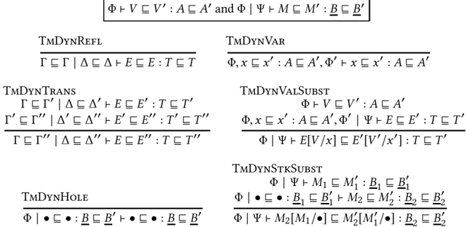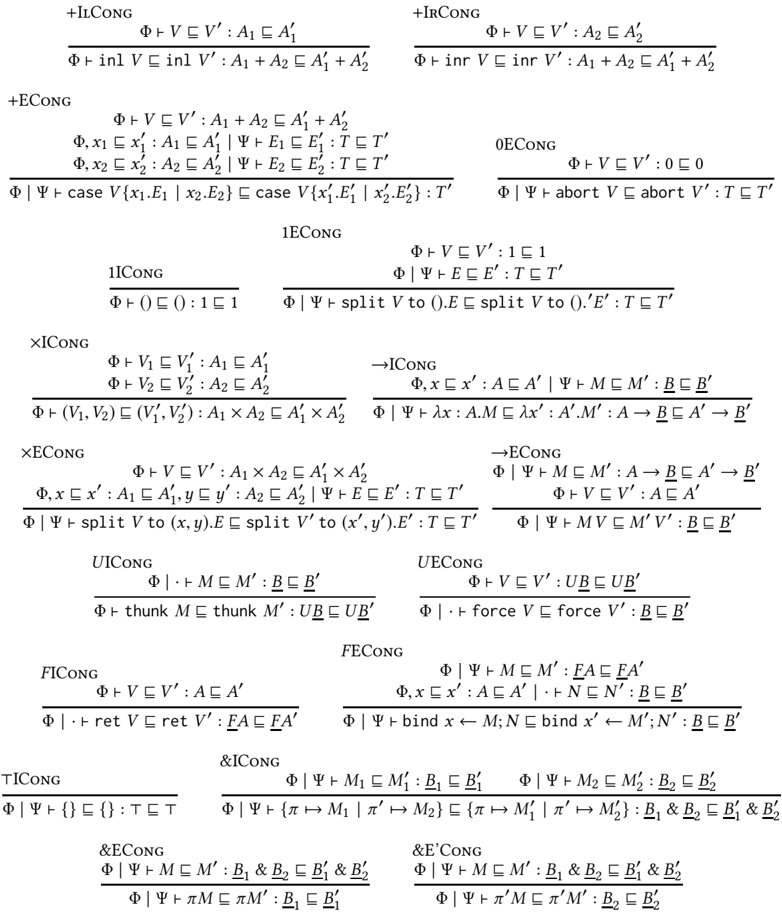The main point of our rules for term dynamism is that there are no type-specific axioms in the definition beyond the βη -axioms that the type satisfies in a non-gradual language. Thus, adding a new type to gradual type theory does not require any a priori consideration of its gradual behavior in the language definition; instead, this is deduced as a theorem in the type theory. The basic structural rules of term dynamism in Figure 3 and Figure 4 say that it is reflexive and transitive ( TmDynRefl , TmDynTrans ), that assumptions can be used and substituted for ( TmDynVar , TmDynValSubst , TmDynHole , TmDynStkSubst ), and that every term constructor is monotone (the Cong rules). While we could add congruence rules for errors and casts, these follow from the axioms characterizing their behavior below. We will often abbreviate a 'homogeneous' term dynamism (where the type or context dynamism is given by reflexivity) by writing e.g. Γ /turnstileleft V /subsetsqequal V ′ : A /subsetsqequal A ′ for Γ /subsetsqequal Γ /turnstileleft V /subsetsqequal V ′ : A /subsetsqequal A ′ , or Φ /turnstileleft V /subsetsqequal V ′ : A for Φ /turnstileleft V /subsetsqequal V ′ : A /subsetsqequal A , and similarly for computations. The entirely homogeneous judgements Γ /turnstileleft V /subsetsqequal V ′ : A and Γ | ∆ /turnstileleft M /subsetsqequal M ′ : B can be thought of as a syntax for contextual error approximation (as we prove below). We write V /supersetsqequal /subsetsqequal V ′ ('equidynamism') to mean term dynamism relations in both directions (which requires that the types are also equidynamic Γ /supersetsqequal /subsetsqequal Γ ′ and A /subsetsqequal A ′ ), which is a syntactic judgement for contextual equivalence. 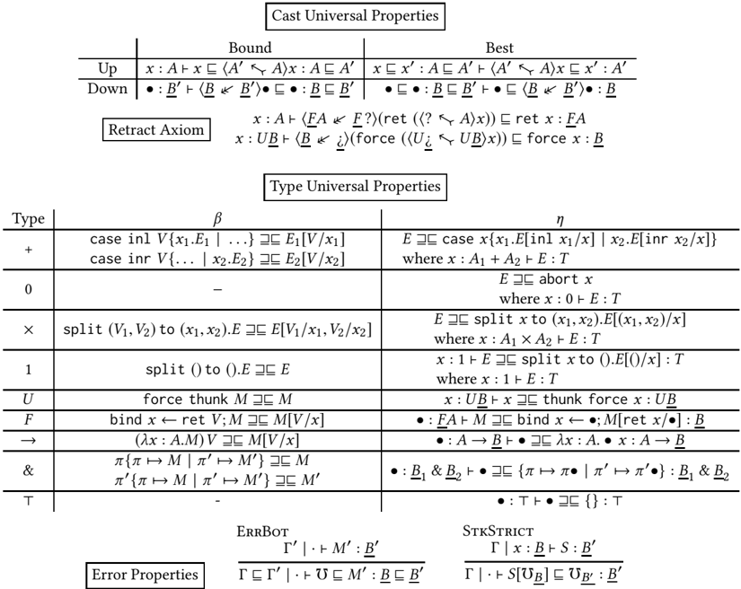## 2.6 Term Dynamism: Axioms Finally, we assert some term dynamism axioms that describe the behavior of programs. The cast universal properties at the top of Figure 5, following New and Licata [2018], say that the defining property of an upcast from A to A ′ is that it is the least dynamic term of type A ′ that is more dynamic that x , a 'least upper bound'. That is, 〈 A ′ /arrowtailleft A 〉 x is a term of type A ′ that is more dynamic that x (the 'bound' rule), and for any other term x ′ of type A ′ that is more dynamic than x , 〈 A ′ /arrowtailleft A 〉 x is less dynamic than x ′ (the 'best' rule). Dually, the downcast 〈 B /dblarrowheadleft B ′ 〉· is the most dynamic term of type B that is less dynamic than · , a 'greatest lower bound'. These defining properties are entirely independent of the types involved in the casts, and do not change as we add or remove types from the system. Wewill show that these defining properties already imply that the shift of the upcast 〈 A ′ /arrowtailleft A 〉 forms a Galois connection/adjunction with the downcast 〈 FA /dblarrowheadleft FA ′ 〉 , and dually for computation types (see Theorem 3.9). They do not automatically form a Galois insertion/coreflection/embeddingprojection pair, but we can add this by the retract axioms in Figure 5. Together with other theorems of GTT, these axioms imply that any upcast followed by its corresponding downcast is the identity (see Theorem 3.10). This specification of casts leaves some behavior undefined: for example, we cannot prove in the theory that 〈 F 1 + 1 /dblarrowheadleft F ? 〉〈 ? /arrowtailleft 1 〉 reduces to an error. We choose this design because there are valid models in which it is not an error, for instance if the unique value of 1 is represented as the boolean true . In Section 4.2, we show additional axioms that fully characterize the behavior of the dynamic type. The type universal properties in the middle of the figure, which are taken directly from CBPV, assert the βη rules for each type as (homogeneous) term equidynamisms-these should be understood as having, as implicit premises, the typing conditions that make both sides type check, in equidynamic contexts. Fig. 5. GTT Term Dynamism Axioms <details> <summary>Image 4 Details</summary>  ### Visual Description ## Logical Rules: Type Systems and Properties ### Overview The image presents a collection of logical rules, likely related to type systems or program semantics. These rules are expressed using mathematical notation and logical symbols, defining relationships between types, expressions, and contexts. The rules are grouped into categories such as "Cast Universal Properties", "Type Universal Properties", and "Error Properties". ### Components/Axes **1. Cast Universal Properties:** - Located at the top of the image. - Subdivided into "Bound" and "Best" categories. - Contains rules involving type casting or subtyping, denoted by symbols like "⊢" and "⊏". **2. Retract Axiom:** - Located below "Cast Universal Properties". - Presents axioms related to retracting or unwrapping types. **3. Type Universal Properties:** - Located in the center of the image. - Organized in a table format with columns for "Type", "β" (beta reduction), and "η" (eta conversion). - Lists rules for various types such as +, 0, ×, 1, U, F, →, &, and ⊤. **4. Error Properties:** - Located at the bottom of the image. - Contains rules related to error handling or type checking in erroneous situations. - Includes labels "ERRBOT" and "STKSTRICT". ### Detailed Analysis or ### Content Details **Cast Universal Properties:** * **Up (Bound):** x: A ⊢ x ⊏ (A' ⇦ A) x: A ⊏ A' * **Up (Best):** x ⊏ x': A ⊏ A' ⊢ (A' ⇦ A) x ⊏ x': A' * **Down (Bound):** •: B' ⊢ (B ⇦ B') • ⊏: B ⊏ B' * **Down (Best):** • ⊏: B ⊏ B' ⊢ (B ⇦ B') •: B **Retract Axiom:** * x: A ⊢ (FA ⇐ F?) (ret (? ⇐ A) x)) ⊏ ret x: FA * x: UB ⊢ (B ⇐) (force (U¿ ⊏ UB) x)) ⊏ force x: B **Type Universal Properties:** | Type | β AND THE LIST GOES ON! </details> The final axioms assert properties of the run-time error term /Omegainv : it is the least dynamic term (has the fewest behaviors) of every computation type, and all complex stacks are strict in errors, because stacks force their evaluation position. We state the first axiom in a heterogeneous way, which includes congruence Γ /subsetsqequal Γ ′ /turnstileleft /Omegainv B /subsetsqequal /Omegainv B ′ : B /subsetsqequal B ′ . ## 3 THEOREMS IN GRADUAL TYPE THEORY In this section, we show that the axiomatics of gradual type theory determine most properties of casts, which shows that these behaviors of casts are forced in any implementation of gradual typing satisfying graduality and β , η . ## 3.1 Properties inherited from CBPV Because the GTT term equidynamism relation /supersetsqequal /subsetsqequal includes the congruence and βη axioms of the CBPV equational theory, types inherit the universal properties they have there [Levy 2003]. We recall some relevant definitions and facts. Definition 3.1 (Isomorphism). - (1) We write A /simequal v A ′ for a value isomorphism between A and A ′ , which consists of two complex values x : A /turnstileleft V ′ : A ′ and x ′ : A ′ /turnstileleft V : A such that x : A /turnstileleft V [ V ′ / x ′ ] /supersetsqequal /subsetsqequal x : A and x ′ : A ′ /turnstileleft V ′ [ V / x ] /supersetsqequal /subsetsqequal x ′ : A ′ . - (2) We write B /simequal c B ′ for a computation isomorphism between B and B ′ , which consists of two complex stacks · : B /turnstileleft S ′ : B ′ and · ′ : B ′ /turnstileleft S : B such that · : B /turnstileleft S [ S ′ / x ′ ] /supersetsqequal /subsetsqequal · : B and · ′ : B ′ /turnstileleft S ′ [ S /·] /supersetsqequal/subsetsqequal · ′ : B ′ . Note that a value isomorphism is a strong condition, and an isomorphism in call-by-value between types A and A ′ corresponds to a computation isomorphism FA /simequal FA ′ , and dually [Levy 2017]. Lemma 3.2 (Initial objects). - (1) For all (value or computation) types T , there exists a unique expression x : 0 /turnstileleft E : T . - (2) For all B , there exists a unique stack · : F 0 /turnstileleft S : B . - (3) 0 is strictly initial: Suppose there is a type A with a complex value x : A /turnstileleft V : 0 . Then V is an isomorphism A /simequal v 0 . - (4) F 0 is not provably strictly initial among computation types. Proof. - (1) Take E to be x : 0 /turnstileleft abort x : T . Given any E ′ , we have E /supersetsqequal /subsetsqequal E ′ by the η principle for 0. - (2) Take S to be · : F 0 /turnstileleft bind x ← · ; abort x : B . Given another S ′ , by the η principle for F types, S ′ /supersetsqequal /subsetsqequal bind x ← · ; S ′ [ ret x ] . By congruence, to show S /supersetsqequal /subsetsqequal S ′ , it suffices to show x : 0 /turnstileleft abort x /supersetsqequal /subsetsqequal S [ ret x ] : B , which is an instance of the previous part. - (3) We have y : 0 /turnstileleft abort y : A . The composite y : 0 /turnstileleft V [ abort y / x ] : 0 is equidynamic with y by the η principle for 0, which says that any two complex values with domain 0 are equal. The composite x : A /turnstileleft abort V : A is equidynamic with x , because <!-- formula-not-decoded --> where the first is by η with x : A , y : A , z : 0 /turnstileleft E [ z ] : = x : A and the second with x : 0 , y : 0 /turnstileleft E [ z ] : = y : A (this depends on the fact that 0 is 'distributive', i.e. Γ , x : 0 has the universal property of 0). Substituting abort V for y and V for z , we have abort V /supersetsqequal /subsetsqequal x . - (4) F 0 is not strictly initial among computation types, though. Proof sketch: a domain model along the lines of [New and Licata 2018] with only non-termination and type errors shows this, because there F 0 and /latticetop are isomorphic (the same object is both initial and terminal), so if F 0 were strictly initial (any type B with a stack · : B /turnstileleft S : F 0 is isomorphic to F 0), then because every type B has a stack to /latticetop (terminal) and therefore F 0, every type would be isomorphic to /latticetop / F 0-i.e. the stack category would be trivial. But there are non-trivial computation types in this model. /square ## Lemma 3.3 (Terminal objects). - (1) For any computation type B , there exists a unique stack · : B /turnstileleft S : /latticetop . - (2) (In any context Γ ,) there exists a unique complex value V : U /latticetop . - (3) (In any context Γ ,) there exists a unique complex value V : 1 . - (4) U /latticetop /simequal v 1 - (5) /latticetop is not a strict terminal object. ## Proof. - (1) Take S = {} . The η rule for /latticetop , · : /latticetop /turnstileleft · /supersetsqequal/subsetsqequal {} : /latticetop , under the substitution of · : B /turnstileleft S : /latticetop , gives S /supersetsqequal /subsetsqequal {}[ S /·] = {} . - (2) Take V = thunk {} . We have x : U /latticetop /turnstileleft x /supersetsqequal /subsetsqequal thunk force x /supersetsqequal /subsetsqequal thunk {} : U /latticetop by the η rules for U and /latticetop . - (3) Take V = () . By η for 1 with x : 1 /turnstileleft E [ x ] : = () : 1, we have x : 1 /turnstileleft () /supersetsqequal/subsetsqequal unroll x to roll () . : 1. By η fro 1 with x : 1 /turnstileleft E [ x ] : = x : 1, we have x : 1 /turnstileleft x /supersetsqequal /subsetsqequal unroll x to roll () . . Therefore x : 1 /turnstileleft x /supersetsqequal /subsetsqequal () : 1. - (4) We have maps x : U /latticetop /turnstileleft () : 1 and x : 1 /turnstileleft thunk {} : U /latticetop . The composite on 1 is the identity by the previous part. The composite on /latticetop is the identity by part (2). - (5) Proof sketch: As above, there is a domain model with /latticetop /simequal F 0, so if /latticetop were a strict terminal object, then F 0 would be too. But F 0 is also initial, so it has a map to every type, and therefore every type would be isomorphic to F 0 and /latticetop . But there are non-trivial computation types in the model. /square ## 3.2 Derived Cast Rules As noted above, monotonicity of type dynamism for U and F means that we have the following as instances of the general cast rules: Lemma 3.4 (Shifted Casts). The following are derivable: <!-- formula-not-decoded --> Proof. They are instances of the general upcast and downcast rules, using the fact that U and F are congruences for type dynamism, so in the first rule FA /subsetsqequal FA ′ , and in the second, UB /subsetsqequal UB ′ . /square The cast universal properties in Figure 5 imply the following seemingly more general rules for reasoning about casts: Lemma 3.5 (Upcast and downcast left and right rules). The following are derivable: <!-- formula-not-decoded --> In sequent calculus terminology, an upcast is left-invertible, while a downcast is right-invertible, in the sense that any time we have a conclusion with a upcast on the left/downcast on the right, we can without loss of generality apply these rules (this comes from upcasts and downcasts forming a Galois connection). We write the A /subsetsqequal A ′ and B ′ /subsetsqequal B ′′ premises on the non-invertible rules to emphasize that the premise is not necessarily well-formed given that the conclusion is. Proof. For upcast left, substitute V ′ into the axiom x /subsetsqequal 〈 A ′′ /arrowtailleft A ′ 〉 x : A ′ /subsetsqequal A ′′ to get V ′ /subsetsqequal 〈 A ′′ /arrowtailleft A ′ 〉 V ′ , and then use transitivity with the premise. For upcast right, by transitivity of <!-- formula-not-decoded --> we have <!-- formula-not-decoded --> Substituting the premise into this gives the conclusion. For downcast left, substituting M ′ into the axiom 〈 B /dblarrowheadleft B ′ 〉· /subsetsqequal · : B /subsetsqequal B ′ gives 〈 B /dblarrowheadleft B ′ 〉 M /subsetsqequal M , and then transitivity with the premise gives the result. For downcast right, transitivity of <!-- formula-not-decoded --> gives · /subsetsqequal · ′′ : B /subsetsqequal B ′′ /turnstileleft · /subsetsqequal 〈 B ′ /dblarrowheadleft B ′′ 〉· ′′ , and then substitution of the premise into this gives the conclusion. /square Though we did not include congruence rules for casts in Figure 4, it is derivable: Lemma 3.6 (Cast congruence rules). The following congruence rules for casts are derivable: <!-- formula-not-decoded --> <!-- formula-not-decoded --> <!-- formula-not-decoded --> Proof. In all cases, uses the invertible and then non-invertible rule for the cast. For the first rule, by upcast left, it suffices to show x /subsetsqequal x ′ : A /subsetsqequal A ′ /turnstileleft x /subsetsqequal 〈 A ′′ /arrowtailleft A ′ 〉 x ′ : A /subsetsqequal A ′′ which is true by upcast right, using x /subsetsqequal x ′ in the premise. For the second, by upcast left, it suffices to show x : A /turnstileleft x /subsetsqequal 〈 A ′′ /arrowtailleft A 〉 x : A /subsetsqequal A ′′ , which is true by upcast right. For the third, by downcast right, it suffices to show · ′ /subsetsqequal · ′′ : B ′ /subsetsqequal B ′′ /turnstileleft 〈 B /dblarrowheadleft B ′ 〉· ′ /subsetsqequal · ′′ : B /subsetsqequal B ′′ , which is true by downcast left, using · ′ /subsetsqequal · ′′ in the premise. For the fourth, by downcast right, it suffices show 〈 B /dblarrowheadleft B ′′ 〉· ′′ /subsetsqequal · ′′ : B /subsetsqequal B ′′ , which is true by downcast left. /square ## 3.3 Type-generic Properties of Casts The universal property axioms for upcasts and downcasts in Figure 5 define them uniquely up to equidynamism ( /supersetsqequal /subsetsqequal ): anything with the same property is behaviorally equivalent to a cast. Theorem 3.7 (Specification for Casts is a Universal Property). - (1) If A /subsetsqequal A ′ and x : A /turnstileleft V : A ′ is a complex value such that x : A /turnstileleft x /subsetsqequal V : A /subsetsqequal A ′ and x /subsetsqequal x ′ : A /subsetsqequal A ′ /turnstileleft V /subsetsqequal x ′ : A ′ then x : A /turnstileleft V /supersetsqequal /subsetsqequal 〈 A ′ /arrowtailleft A 〉 x : A ′ . - (2) If B /subsetsqequal B ′ and · ′ : B ′ /turnstileleft S : B is a complex stack such that · ′ : B ′ /turnstileleft S /subsetsqequal · ′ : B /subsetsqequal B ′ and · /subsetsqequal · ′ : B /subsetsqequal B ′ /turnstileleft · /subsetsqequal S : B then · ′ : B ′ /turnstileleft S /supersetsqequal /subsetsqequal 〈 B /dblarrowheadleft B ′ 〉· ′ : B Proof. For the first part, to show 〈 A ′ /arrowtailleft A 〉 x /subsetsqequal V , by upcast left, it suffices to show x /subsetsqequal V : A /subsetsqequal A ′ , which is one assumption. To show V /subsetsqequal 〈 A ′ /arrowtailleft A 〉 x , we substitute into the second assumption with x /subsetsqequal 〈 A ′ /arrowtailleft A 〉 x : A /subsetsqequal A ′ , which is true by upcast right. For the second part, to show S /subsetsqequal 〈 B /dblarrowheadleft B ′ 〉· ′ , by downcast right, it suffices to show S /subsetsqequal · ′ : B /subsetsqequal B ′ , which is one of the assumptions. To show 〈 B /dblarrowheadleft B ′ 〉· ′ /subsetsqequal S , we substitute into the second assumption with 〈 B /dblarrowheadleft B ′ 〉· ′ /subsetsqequal · ′ , which is true by downcast left. /square Casts satisfy an identity and composition law: Theorem 3.8 (Casts (de)composition). For any A /subsetsqequal A ′ /subsetsqequal A ′′ and B /subsetsqequal B ′ /subsetsqequal B ′′ : - (1) x : A /turnstileleft 〈 A /arrowtailleft A 〉 x /supersetsqequal /subsetsqequal x : A - (2) x : A /turnstileleft 〈 A ′′ /arrowtailleft A 〉 x /supersetsqequal /subsetsqequal 〈 A ′′ /arrowtailleft A ′ 〉〈 A ′ /arrowtailleft A 〉 x : A ′′ - (3) · : B /turnstileleft 〈 B /dblarrowheadleft B 〉· /supersetsqequal/subsetsqequal · : B - (4) · : B ′′ /turnstileleft 〈 B /dblarrowheadleft B ′′ 〉· /supersetsqequal/subsetsqequal 〈 B /dblarrowheadleft B ′ 〉(〈 B ′ /dblarrowheadleft B ′′ 〉·) : B /subsetsqequal B Proof. We use Theorem 3.7 in all cases, and show that the right-hand side has the universal property of the left. - (1) Both parts expand to showing x /subsetsqequal x : A /subsetsqequal A /turnstileleft x /subsetsqequal x : A /subsetsqequal A , which is true by assumption. - (2) First, we need to show x /subsetsqequal 〈 A ′′ /arrowtailleft A ′ 〉(〈 A ′ /arrowtailleft A 〉 x ) : A /subsetsqequal A ′′ . By upcast right, it suffices to show x /subsetsqequal 〈 A ′ /arrowtailleft A 〉 x : A /subsetsqequal A ′ , which is also true by upcast right. For x /subsetsqequal x ′′ : A /subsetsqequal A ′′ /turnstileleft 〈 A ′′ /arrowtailleft A ′ 〉(〈 A ′ /arrowtailleft A 〉 x ) /subsetsqequal x ′′ , by upcast left twice, it suffices to show x /subsetsqequal x ′′ : A /subsetsqequal A ′′ , which is true by assumption. - (3) Both parts expand to showing · : B /turnstileleft · /subsetsqequal · : B , which is true by assumption. - (4) To show · /subsetsqequal · ′′ : B /subsetsqequal B ′′ /turnstileleft · /subsetsqequal 〈 B /dblarrowheadleft B ′ 〉(〈 B ′ /dblarrowheadleft B ′′ 〉·) , by downcast right (twice), it suffices to show · : B /subsetsqequal · ′′ : B ′′ /turnstileleft · /subsetsqequal · ′′ : B /subsetsqequal B ′′ , which is true by assumption. Next, we have to show 〈 B /dblarrowheadleft B ′ 〉(〈 B ′ /dblarrowheadleft B ′′ 〉·) /subsetsqequal · : B /subsetsqequal B ′′ , and by downcast left, it suffices to show 〈 B ′ /dblarrowheadleft B ′′ 〉· /subsetsqequal · : B ′ /subsetsqequal B ′′ , which is also true by downcast left. /square In particular, this composition property implies that the casts into and out of the dynamic type are coherent, for example if A /subsetsqequal A ′ then 〈 ? /arrowtailleft A 〉 x /supersetsqequal /subsetsqequal 〈 ? /arrowtailleft A ′ 〉〈 A ′ /arrowtailleft A 〉 x . The following theorem says essentially that x /subsetsqequal 〈 T /dblarrowheadleft T ′ 〉〈 T ′ /arrowtailleft T 〉 x (upcast then downcast might error less but but otherwise does not change the behavior) and 〈 T ′ /arrowtailleft T 〉〈 T /dblarrowheadleft T ′ 〉 x /subsetsqequal x (downcast then upcast might error more but otherwise does not change the behavior). However, since a value type dynamism A /subsetsqequal A ′ induces a value upcast x : A /turnstileleft 〈 A ′ /arrowtailleft A 〉 x : A ′ but a stack downcast · : FA ′ /turnstileleft 〈 FA /dblarrowheadleft FA ′ 〉· : FA (and dually for computations), the statement of the theorem wraps one cast with the constructors for U and F types (functoriality of F / U ). Theorem 3.9 (Casts are a Galois Connection). - (1) · ′ : FA ′ /turnstileleft bind x ←〈 FA /dblarrowheadleft FA ′ 〉· ′ ; ret (〈 A ′ /arrowtailleft A 〉 x ) /subsetsqequal · ′ : FA ′ - (3) x : UB ′ /turnstileleft 〈 UB ′ /arrowtailleft UB 〉( thunk (〈 B /dblarrowheadleft B ′ 〉 force x )) /subsetsqequal x : UB ′ - (2) · : FA /turnstileleft · /subsetsqequal bind x ←· ; 〈 FA /dblarrowheadleft FA ′ 〉( ret (〈 A ′ /arrowtailleft A 〉 x )) : FA - (4) x : UB /turnstileleft x /subsetsqequal thunk (〈 B /dblarrowheadleft B ′ 〉( force (〈 UB ′ /arrowtailleft UB 〉 x ))) : UB Proof. - (1) By η for F types, · ′ : FA ′ /turnstileleft · ′ /supersetsqequal /subsetsqequal bind x ′ ←· ′ ; ret x ′ : FA ′ , so it suffices to show <!-- formula-not-decoded --> By congruence, it suffices to show 〈 FA /dblarrowheadleft FA ′ 〉· ′ /subsetsqequal · ′ : FA /subsetsqequal FA ′ , which is true by downcast left, and x /subsetsqequal x ′ : A /subsetsqequal A ′ /turnstileleft ret (〈 A ′ /arrowtailleft A 〉 x ) /subsetsqequal ret x ′ : A ′ , which is true by congruence for ret , upcast left, and the assumption. - (2) By η for F types, it suffices to show <!-- formula-not-decoded --> so by congruence, <!-- formula-not-decoded --> By downcast right, it suffices to show <!-- formula-not-decoded --> <!-- formula-not-decoded --> which is true by upcast right. - (3) By η for U types, it suffices to show <!-- formula-not-decoded --> and by congruence By upcast left, it suffices to show <!-- formula-not-decoded --> and by congruence <!-- formula-not-decoded --> which is true by downcast left. - (4) By η for U types, it suffices to show <!-- formula-not-decoded --> and by congruence <!-- formula-not-decoded --> By downcast right, it suffices to show <!-- formula-not-decoded --> and by congruence <!-- formula-not-decoded --> which is true by upcast right. /square The retract property says roughly that x /supersetsqequal /subsetsqequal 〈 T ′ /dblarrowheadleft T 〉〈 T ′ /arrowtailleft T 〉 x (upcast then downcast does not change the behavior), strengthening the /subsetsqequal of Theorem 3.9. In Figure 5, we asserted the retract axiom for casts with the dynamic type. This and the composition property implies the retraction property for general casts: Theorem 3.10 (Retract Property for General Casts). <!-- formula-not-decoded --> Proof. We need only to show the /subsetsqequal direction, because the converse is Theorem 3.9. - (1) Substituting ret (〈 A ′ /arrowtailleft A 〉 x ) into Theorem 3.9's <!-- formula-not-decoded --> and β -reducing gives <!-- formula-not-decoded --> Using this, after η -expanding · : FA on the right and using congruence for bind , it suffices to derive as follows: <!-- formula-not-decoded --> - (2) After using η for U and congruence, it suffices to show <!-- formula-not-decoded --> <!-- formula-not-decoded --> ``` ``` /square ## 3.4 Unique Implementations of Casts Definition 3.11. Let a type constructor C be a (value or computation) type that well-formed according to the grammar in Figure 1 with additional hypotheses X val type and Y comp type standing for value or computation types, respectively. We write C [ A / X ] and C [ B / Y ] for the substitution of a type for a variable. For example, are type constructors. It is admissible that all type constructors are monotone in type dynamism, because we included a congruence rule for every type constructor in Figure 2: Lemma 3.12 (Monotonicity of Type Constructors). For any type constructor X val type /turnstileleft C , if A /subsetsqequal A ′ then C [ A / X ] /subsetsqequal C [ A ′ / x ] . For any type constructor Y comp type /turnstileleft C , if B /subsetsqequal B ′ then C [ B / Y ] /subsetsqequal C [ B ′ / Y ] . Proof. Induction on C . In the case for a variable X or Y , A /subsetsqequal A ′ or B /subsetsqequal B ′ by assumption. In all other cases, the result follows from the inductive hypotheses and the congruence rule for type dynamism for the type constructor (Figure 2). For example, in the case for + , A 1 [ A / x ] /subsetsqequal A 1 [ A ′ / x ] and A 2 [ A / x ] /subsetsqequal A 2 [ A ′ / x ] , so A 1 [ A / x ] + A 2 [ A / x ] /subsetsqequal A 1 [ A ′ / x ] + A 2 [ A ′ / x ] . /square The following lemma helps show that a complex value 〈 〈 C [ A ′ i / X i , B ′ i / Y i ] /arrowtailleft C [ A i / X i , B i / Y i ]〉 〉 is an upcast from C [ A i / X i , B i / Y i ] to C [ A ′ i / X i , B ′ i / Y i ] . Lemma3.13(UpcastLemma). Let X 1 val type , . . . X n val type , Y 1 comp type , . . . Y n comp type /turnstileleft C val type be a value type constructor. We abbreviate the instantiation <!-- formula-not-decoded --> Suppose 〈〈 C [ A ′ i , B ′ i ] /arrowtailleft C [ A i , B i ]〉〉-is a complex value (depending on C and each A i , A ′ i , B i , B ′ i ) such that - (1) For all value types A 1 , . . . , A n and A ′ 1 , . . . , A ′ n with A i /subsetsqequal A ′ i , and all computation types B 1 , . . . , B m and B ′ 1 , . . . , B ′ n with B i /subsetsqequal B ′ i , <!-- formula-not-decoded --> - (2) For all value types A i /subsetsqequal A ′ i and computation types B i /subsetsqequal B ′ i , <!-- formula-not-decoded --> ``` ``` - (3) For all value types A 1 , . . . , A n and all computation types B 1 , . . . , B m , <!-- formula-not-decoded --> Then 〈 〈 C [ A ′ i , B ′ i ] /arrowtailleft C [ A i , B i ]〉 〉 satisfies the universal property of an upcast, so by Theorem 3.7 <!-- formula-not-decoded --> Moreover, the left-to-right direction uses only the left-to-right direction of assumption (3), and the right-to-left uses only the right-to-left direction of assumption (3). Proof. First, we show that 〈〈 C [ A ′ i , B ′ i ] /arrowtailleft C [ A i , B i ]〉〉 satisfies the universal property of an upcast. To show <!-- formula-not-decoded --> assumption (2) part 2 gives <!-- formula-not-decoded --> Then transitivity with the left-to-right direction of assumption (3) <!-- formula-not-decoded --> gives the result. To show <!-- formula-not-decoded --> By assumption (2) part 1, we have <!-- formula-not-decoded --> so transitivity with the right-to-left direction of assumption (3) gives the result: <!-- formula-not-decoded --> ThenTheorem3.7implies that 〈 〈 C [ A ′ i , B ′ i ] /arrowtailleft C [ A i , B i ]〉 〉 is equivalent to 〈 C [ A ′ i , B ′ i ] /arrowtailleft C [ A i , B i ]〉 . /square Dually, we have Lemma3.14(DowncastLemma). Let X 1 val type , . . . X n val type , Y 1 comp type , . . . Y n comp type /turnstileleft C comp type be a computation type constructor. We abbreviate the instantiation <!-- formula-not-decoded --> Suppose 〈〈 C [ A i , B i ] /dblarrowheadleft C [ A ′ i , B ′ i ]〉〉-is a complex stack (depending on C and each A i , A ′ i , B i , B ′ i ) such that - (1) For all value types A 1 , . . . , A n and A ′ 1 , . . . , A ′ n with A i /subsetsqequal A ′ i , and all computation types B 1 , . . . , B m and B ′ 1 , . . . , B ′ n with B i /subsetsqequal B ′ i , <!-- formula-not-decoded --> - (2) For all value types A i /subsetsqequal A ′ i and computation types B i /subsetsqequal B ′ i , <!-- formula-not-decoded --> - (3) For all value types A 1 , . . . , A n and all computation types B 1 , . . . , B m , <!-- formula-not-decoded --> Then 〈 〈 C [ A i , B i ] /dblarrowheadleft C [ A ′ i , B ′ i ]〉 〉 satisfies the universal property of a downcast, so by Theorem 3.7 <!-- formula-not-decoded --> Moreover, the left-to-right direction uses only the left-to-right direction of assumption (3), and the right-to-left uses only the right-to-left direction of assumption (3). Proof. First, we show that 〈 C [ A i , B i ] /dblarrowheadleft C [ A ′ i , B ′ i ]〉 satisfies the universal property of a downcast, and then apply Theorem 3.7. To show <!-- formula-not-decoded --> assumption (2) part 2 gives <!-- formula-not-decoded --> Then transitivity with the right-to-left direction of assumption (3) <!-- formula-not-decoded --> <!-- formula-not-decoded --> by assumption (2) part 1, we have <!-- formula-not-decoded --> so transitivity with the left-to-right direction of assumption (3) <!-- formula-not-decoded --> gives the result. To show gives the result. /square Together, the universal property for casts and the η principles for each type imply that the casts must behave as in lazy cast semantics: Theorem 3.15 (Cast Uni/q.sc\_u.sce Implementation Theorem for + , × , → , & ). The casts' behavior is uniquely determined as follows: <!-- formula-not-decoded --> <!-- formula-not-decoded --> In the case for an eager product × , we can actually also show that reversing the order and running 〈 FA 2 /dblarrowheadleft FA ′ 2 〉 ret x ′ 2 and then 〈 FA 1 /dblarrowheadleft FA ′ 1 〉 ret x ′ 1 is also an implementation of this cast, and therefore equal to the above. Intuitively, this is sensible because the only effect a downcast introduces is a run-time error, and if either downcast errors, both possible implementations will. Proof. - (1) Sums upcast. We use Lemma 3.13 with the type constructor X 1 val type , X 2 val type /turnstileleft X 1 + X 2 val type. Suppose A 1 /subsetsqequal A ′ 1 and A 2 /subsetsqequal A ′ 2 and let <!-- formula-not-decoded --> stand for <!-- formula-not-decoded --> which has the type required for the lemma's assumption (1). Assumption (2) requires two condition, both of which are proved by the congruence rules for case , inl , inr , and upcasts. The first, <!-- formula-not-decoded --> • /subsetsqequal • ′ The second, <!-- formula-not-decoded --> expands to <!-- formula-not-decoded --> Finally, for assumption (3), we need to show <!-- formula-not-decoded --> which is true because 〈 A 1 /arrowtailleft A 1 〉 and 〈 A 2 /arrowtailleft A 2 〉 are the identity, and using 'weak η ' for sums, case s { x 1 . inl x 1 | x 2 . inr x 2 } /supersetsqequal /subsetsqequal x , which is the special case of the η rule in Figure 5 for the identity complex value: <!-- formula-not-decoded --> - (2) Sumsdowncast. We use the downcast lemma with X 1 val type , X 2 val type /turnstileleft F ( X 1 + X 2 ) comp type. Let <!-- formula-not-decoded --> stand for <!-- formula-not-decoded --> (where, as in the theorem statement, inr branch is analogous), which has the correct type for the lemma's assumption (1). For assumption (2), we first need to show - : F ( A ′ 1 + A ′ 2 ) /turnstileleft 〈 〈 F ( A 1 + A 2 ) /dblarrowheadleft F ( A ′ 1 + A ′ 2 )〉 〉· ′ /subsetsqequal 〈 〈 F ( A ′ 1 + A ′ 2 ) /dblarrowheadleft F ( A ′ 1 + A ′ 2 )〉 〉· ′ : F ( A 1 + A 2 ) /subsetsqequal F ( A ′ 1 + A ′ 2 ) i.e. <!-- formula-not-decoded --> /subsetsqequal <!-- formula-not-decoded --> which is true by the congruence rules for bind , case , downcasts, ret , and inl / inr . Next, we need to show : F ( A i.e. <!-- formula-not-decoded --> which is also true by congruence. Finally, for assumption (3), we show <!-- formula-not-decoded --> • + A ) /subsetsqequal F ( A ′ + A ′ ) /turnstileleft 〈 〈 F ( A + A ) /dblarrowheadleft F ( A + A )〉 〉• /subsetsqequal 〈 〈 F ( A + A ) /dblarrowheadleft F ( A ′ + A ′ )〉 〉• ′ : F using the downcast identity, β for F types, η for sums, and η for F types. ( A + A ) - (3) Eager product upcast. We use Lemma 3.13 with the type constructor X 1 val type , X 2 val type /turnstileleft X 1 × X 2 val type. Let <!-- formula-not-decoded --> <!-- formula-not-decoded --> which has the type required for the lemma's assumption (1). Assumption (2) requires two condition, both of which are proved by the congruence rules for split , pairing, and upcasts. The first, <!-- formula-not-decoded --> expands to The second, /subsetsqequal p A A × : ′ expands to p stand for /subsetsqequal A <!-- formula-not-decoded --> <!-- formula-not-decoded --> ′ A A A A A s A A A × /turnstileleft 〈 〈 × × 〉 〉 /subsetsqequal 〈 〈 × /arrowtailleft /arrowtailleft ′ ′ ′ ′ ′ <!-- formula-not-decoded --> <!-- formula-not-decoded --> <!-- formula-not-decoded --> Finally, for assumption (3), using η for products and the fact that 〈 A /arrowtailleft A 〉 is the identity, we have <!-- formula-not-decoded --> - (4) Eager product downcast. We use the downcast lemma with X 1 val type , X 2 val type /turnstileleft F ( X 1 × X 2 ) comp type. Let <!-- formula-not-decoded --> stand for <!-- formula-not-decoded --> which has the correct type for the lemma's assumption (1). For assumption (2), we first need to show - : F ( A ′ 1 × A ′ 2 ) /turnstileleft 〈 〈 F ( A 1 × A 2 ) /dblarrowheadleft F ( A ′ 1 × A ′ 2 )〉 〉· ′ /subsetsqequal 〈 〈 F ( A ′ 1 × A ′ 2 ) /dblarrowheadleft F ( A ′ 1 × A ′ 2 )〉 〉· ′ : F ( A 1 × A 2 ) /subsetsqequal F ( A ′ 1 × A ′ 2 ) i.e. bind p ′ ←• ; split p ′ to ( x ′ FA /subsetsqequal - bind p ′ ←· ; split p ′ to ( x ′ 1 , x ′ 2 ) . bind x ′ 1 ←〈 FA ′ 1 /dblarrowheadleft FA ′ 1 〉 ret x ′ 1 ; bind x ′ 2 ←〈 FA ′ 2 /dblarrowheadleft FA ′ 2 〉 ret x ′ 2 ; ret ( x ′ 1 , x ′ 2 ) which is true by the congruence rules for bind , split , downcasts, ret , and pairing. Next, we need to show - /subsetsqequal · ′ : F ( A 1 × A 2 ) /subsetsqequal F ( A ′ 1 × A ′ 2 ) /turnstileleft 〈 〈 F ( A 1 × A 2 ) /dblarrowheadleft F ( A 1 × A 2 )〉 〉· /subsetsqequal 〈 〈 F ( A 1 × A 2 ) /dblarrowheadleft F ( A ′ 1 × A ′ 2 )〉 〉· ′ : F ( A 1 + A 2 ) i.e. <!-- formula-not-decoded --> /subsetsqequal bind p ′ ←· ; split p ′ to ( x ′ 1 , x ′ 2 ) . bind x 1 ←〈 FA 1 /dblarrowheadleft FA ′ 1 〉 ret x ′ 1 ; bind x 2 ←〈 FA 2 /dblarrowheadleft FA ′ 2 〉 ret x ′ 2 ; ret ( x 1 , x 2 ) which is also true by congruence. , x ′ ) . bind x ←〈 FA /dblarrowheadleft ′ 〉 ret x ′ ; bind x ←〈 FA /dblarrowheadleft FA ′ 〉 ret x ′ ; ret ( ′ × A ′ 〉 〉 s ′ : A ′ × A ′ x , x ) Finally, for assumption (3), we show <!-- formula-not-decoded --> • using the downcast identity, β for F types, η for eager products, and η for F types. An analogous argument works if we sequence the downcasts of the components in the opposite order: <!-- formula-not-decoded --> (the only facts about downcasts used above are congruence and the downcast identity), which shows that these two implementations of the downcast are themselves equidynamic. - (5) Lazy product downcast. We use Lemma3.14 with the type constructor Y 1 comp type , Y 2 comp type /turnstileleft Y 1 & Y 2 val type. Let <!-- formula-not-decoded --> <!-- formula-not-decoded --> which has the type required for the lemma's assumption (1). Assumption (2) requires two conditions, both of which are proved by the congruence rules for pairing, projection, and downcasts. The first, - ′ : B ′ 1 & B ′ 2 /turnstileleft 〈 〈 B 1 & B 2 /dblarrowheadleft B ′ 1 & B ′ 2 〉 〉· ′ /subsetsqequal 〈 〈 B ′ 1 & B ′ 2 /dblarrowheadleft B ′ 1 & B ′ 2 〉 〉· ′ : B 1 & B 2 /subsetsqequal B ′ 1 & B ′ 2 expands to <!-- formula-not-decoded --> <!-- formula-not-decoded --> <!-- formula-not-decoded --> stand for The second, <!-- formula-not-decoded --> expands to stand for <!-- formula-not-decoded --> which has the type required for the lemma's assumption (1). Assumption (2) requires two conditions, both of which are proved by the congruence rules for thunk , force , pairing, projections, and upcasts. The first, <!-- formula-not-decoded --> <!-- formula-not-decoded --> <!-- formula-not-decoded --> For assumption (3), we have, using 〈 B /dblarrowheadleft B 〉 is the identity and η for &, <!-- formula-not-decoded --> - (6) Lazy product upcast. WeuseLemma3.13withthetypeconstructor Y 1 comp type , Y 2 comp type /turnstileleft U ( Y 1 & Y 2 ) val type. Let <!-- formula-not-decoded --> expands to thunk { π ↦→ force (〈 UB 1 /arrowtailleft UB 1 〉( thunk π ( force p ))) | π ′ ↦→ force (〈 UB 2 /arrowtailleft UB 2 〉( thunk π ′ ( force p )))} /subsetsqequal thunk { π ↦→ force (〈 UB ′ 1 /arrowtailleft UB 1 〉( thunk π ( force p ))) | π ′ ↦→ force (〈 UB ′ 2 /arrowtailleft UB 2 〉( thunk π ′ ( force p )))} The second, p /subsetsqequal p ′ : U ( B 1 & B 2 ) /subsetsqequal U ( B ′ 1 & B ′ 2 ) /turnstileleft 〈 〈 U ( B ′ 1 & B ′ 2 ) /arrowtailleft U ( B 1 & B 2 )〉 〉 p /subsetsqequal 〈 〈 U ( B ′ 1 & B ′ 2 ) /arrowtailleft U ( B ′ 1 & B ′ 2 )〉 〉 p : U ( B ′ 1 & B ′ 2 ) expands to thunk { π ↦→ force (〈 UB ′ 1 /arrowtailleft UB 1 〉( thunk π ( force p ))) | π ′ ↦→ force (〈 UB ′ 2 /arrowtailleft UB 2 〉( thunk π ′ ( force p )))} /subsetsqequal thunk { π ↦→ force (〈 UB ′ 1 /arrowtailleft UB ′ 1 〉( thunk π ( force p ′ ))) | π ′ ↦→ force (〈 UB ′ 2 /arrowtailleft UB ′ 2 〉( thunk π ′ ( force p ′ )))} Finally, for assumption (3), using η for times , β and η for U types, and the fact that 〈 A /arrowtailleft A 〉 is the identity, we have thunk { π ↦→ force (〈 UB 1 /arrowtailleft UB 1 〉( thunk π ( force p ))) | π ′ ↦→ force (〈 UB 2 /arrowtailleft UB 2 〉( thunk π ′ ( force p )))} /supersetsqequal /subsetsqequal thunk { π ↦→ force ( thunk π ( force p )) | π ′ ↦→ force ( thunk π ′ ( force p ))} /supersetsqequal /subsetsqequal thunk { π ↦→ π ( force p ) | π ′ ↦→ π ′ ( force p )} /supersetsqequal /subsetsqequal thunk ( force p ) /supersetsqequal /subsetsqequal p ## (7) Function downcast. Weuse Lemma3.14 with the type constructor X val type , Y comp type /turnstileleft X → Y comp type. Let <!-- formula-not-decoded --> <!-- formula-not-decoded --> <!-- formula-not-decoded --> which has the type required for the lemma's assumption (1). Assumption (2) requires two conditions, both of which are proved by the congruence rules for λ , application, upcasts, and downcasts. The first, <!-- formula-not-decoded --> expands to The second, <!-- formula-not-decoded --> expands to stand for <!-- formula-not-decoded --> <!-- formula-not-decoded --> For assumption (3), we have, using 〈 A /arrowtailleft A 〉 and 〈 B /dblarrowheadleft B 〉 are the identity and η for → , <!-- formula-not-decoded --> - (8) Function upcast. ``` ``` /square In GTT, we assert the existence of value upcasts and computation downcasts for derivable type dynamism relations. While we do not assert the existence of all value downcasts and computation upcasts, we can define the universal property that identifies a term as such: Definition 3.16 (Stack upcasts/value downcasts). - (1) If B /subsetsqequal B ′ , a stack upcast from B to B ′ is a stack · : B /turnstileleft 〈〈 B ′ /arrowtailleft B 〉〉· : B ′ that satisfies the computation dynamism rules of an upcast · : B /turnstileleft · /subsetsqequal 〈 〈 B ′ /arrowtailleft B 〉 〉· : B /subsetsqequal B ′ and · /subsetsqequal · ′ : B /subsetsqequal B ′ /turnstileleft 〈 〈 B ′ /arrowtailleft B 〉 〉· /subsetsqequal · ′ : B ′ . - (2) If A /subsetsqequal A ′ , a value downcast from A ′ to A is a complex value x : A ′ /turnstileleft 〈〈 A /dblarrowheadleft A ′ 〉〉 x : A that satisfies the value dynamism rules of a downcast x : A ′ /turnstileleft 〈 〈 A /dblarrowheadleft A ′ 〉 〉 x /subsetsqequal x : A /subsetsqequal A ′ and x /subsetsqequal x ′ : A /subsetsqequal A ′ /turnstileleft x /subsetsqequal 〈 〈 A /dblarrowheadleft A ′ 〉 〉 x ′ : A . <!-- formula-not-decoded --> Because the proofs of Lemma 3.5, Lemma 3.6, Theorem 3.8, Theorem 3.7 rely only on the axioms for upcasts/downcasts, the analogues of these theorems hold for stack upcasts and value downcasts as well.Some value downcasts and computation upcasts do exist, leading to a characterization of the casts for the monad UFA and comonad FUB of F /turnstileright U : Theorem 3.17 (Cast Uni/q.sc\_u.sce Implementation Theorem for UF , FU ). Let A /subsetsqequal A ′ and B /subsetsqequal B ′ . - (1) · : FA /turnstileleft bind x : A ←· ; ret (〈 A ′ /arrowtailleft A 〉 x ) : FA ′ is a stack upcast. <!-- formula-not-decoded --> - (2) If 〈 〈 B ′ /arrowtailleft B 〉 〉 is a stack upcast, then - (3) x : UB ′ /turnstileleft thunk (〈 B /dblarrowheadleft B ′ 〉( force x )) : UB is a value downcast. - (4) If 〈 〈 A /dblarrowheadleft A ′ 〉 〉 is a value downcast, then - : FA ′ /turnstileleft 〈 FA /dblarrowheadleft FA ′ 〉· /supersetsqequal/subsetsqequal bind x ′ : A ′ ←· ; ret (〈 A /dblarrowheadleft A ′ 〉 x ) x : UFA /turnstileleft 〈 UFA ′ /arrowtailleft UFA 〉 x /supersetsqequal /subsetsqequal thunk ( bind x : A ← force x ; ret (〈 A ′ /arrowtailleft A 〉 x )) - (5) · : FUB ′ /turnstileleft 〈 FUB /dblarrowheadleft FUB ′ 〉· /supersetsqequal/subsetsqequal bind x ′ : UB ′ ←· ; ret ( thunk (〈 B /dblarrowheadleft B ′ 〉( force x ))) Proof. ## (1) To show <!-- formula-not-decoded --> we can η -expand · /supersetsqequal /subsetsqequal bind x ← · ; ret x on the left, at which point by congruence it suffices to show x /subsetsqequal 〈 A ′ /arrowtailleft A 〉 x , which is true up upcast right. To show <!-- formula-not-decoded --> we can η -expand · ′ /supersetsqequal /subsetsqequal bind x ′ ←· ′ ; ret x ′ on the right, and then apply congruence, the assumption that · /subsetsqequal · ′ , and upcast left. - (2) Weapply the upcast lemma with the type constructor Y comp type /turnstileleft UY val type. The term thunk (〈 〈 B ′ /arrowtailleft B 〉 〉( force x )) has the correct type for assumption (1). For assumption (2), we show <!-- formula-not-decoded --> by congruence for thunk , 〈 〈 B /arrowtailleft B 〉 〉 (proved analogously to Lemma 3.6), and force . We show <!-- formula-not-decoded --> by congruence as well. Finally, for assumption (3), we have <!-- formula-not-decoded --> <!-- formula-not-decoded --> using η for U types and the identity principle for 〈〈 B /arrowtailleft B 〉〉 (proved analogously to Theorem 3.8). ## (3) To show <!-- formula-not-decoded --> we can η -expand x ′ to thunk force x ′ , and then by congruence it suffices to show 〈 B /dblarrowheadleft B ′ 〉( force x ′ ) /subsetsqequal force x ′ : B /subsetsqequal B ′ , which is downcast left. Conversely, for <!-- formula-not-decoded --> we η -expand x to thunk ( force x ) , and then it suffices to show 〈 B /dblarrowheadleft B ′ 〉( force x ) /subsetsqequal force x ′ , which is true by downcast right and congruence of force on the assumption x /subsetsqequal x ′ . - (4) We use the downcast lemma with X val type /turnstileleft FX comp type, where bind x ′ : A ′ ← · ; ret (〈 〈 A /dblarrowheadleft A ′ 〉 〉 x ) has the correct type for assumption (1). For assumption (2), we show <!-- formula-not-decoded --> by congruence for bind , ret , and 〈〈 A ′ /dblarrowheadleft A ′ 〉〉 (which is proved analogously to Lemma 3.6). We also show - /subsetsqequal · ′ : FA /subsetsqequal FA ′ /turnstileleft bind x : A ←· ; ret (〈 〈 A /dblarrowheadleft A 〉 〉 x ) /subsetsqequal bind x ′ : A ′ ←· ; ret (〈 〈 A /dblarrowheadleft A ′ 〉 〉· ′ ) : FA by congruence. Finally, for assumption (3), we have <!-- formula-not-decoded --> • using the identity principle for 〈 〈 A /dblarrowheadleft A 〉 〉 (proved analogously to Theorem 3.8) and η for F types. - (5) Combining parts (1) and (2) gives the first equation, while combining parts (3) and (4) gives the second equation. /square Recall that for value types A 1 and A 2, the CBV function type is U ( A 1 → FA 2 ) . As a corollary of Theorems 3.15 and 3.17, we have Corollary 3.18 (Cast Uni/q.sc\_u.sce Implementation for CBV Functions). <!-- formula-not-decoded --> <!-- formula-not-decoded --> Proof. For the upcast, by Theorem 3.15, it's equal to <!-- formula-not-decoded --> By Theorem 3.17, 〈 UFA ′ 2 /arrowtailleft UFA 2 〉 is equal to <!-- formula-not-decoded --> so β -reducing force and thunk twice gives the result. For the downcast, by Theorem 3.17, it's equal to <!-- formula-not-decoded --> and by Theorem 3.15 〈( A 1 → FA 2 ) /dblarrowheadleft ( A 1 → FA 2 )〉-is equal to <!-- formula-not-decoded --> These are equivalent to the CBPV translations of the standard CBV wrapping implementations; for example, the CBV upcast term λx ′ . let x = 〈 A 1 /dblarrowheadleft A ′ 1 〉 x ′ ; 〈 A ′ 2 /arrowtailleft A 2 〉( f x ′ ) has its evaluation order made explicit, and the fact that its upcast is a (complex) value exposed. In the downcast, the GTT term is free to let-bind (〈 A ′ 1 /arrowtailleft A 1 〉 x ) to avoid duplicating it, but because it is a (complex) value, it can also be substituted directly, which might expose reductions that can be optimized. ## 3.5 Least Dynamic Types Theorem 3.19 (Least Dynamic Value Type). If ⊥ v is a type such that ⊥ v /subsetsqequal A for all A , then in GTT with a strict initial object 0 , ⊥ v /simequal v 0 . Proof. We have the upcast x : ⊥ v /turnstileleft 〈 0 /arrowtailleft ⊥ v 〉 x : 0, so Lemma 3.2 gives the result. /square The fact that ⊥ v is strictly initial seems to depend on the fact that we have a strictly initial object: In GTT without a 0 type, it seems that we cannot prove that x : ⊥ v /turnstileleft 〈 A /arrowtailleft ⊥ v 〉 x : A is the unique such map. Theorem 3.20 (Least Dynamic Computation Type). If ⊥ c is a type such that ⊥ c /subsetsqequal B for all B , and we have a terminal computation type /latticetop , then U ⊥ c /simequal v U /latticetop . Proof. We have stacks · : /latticetop 〈⊥ c /dblarrowheadleft /latticetop〉 · : ⊥ c and · : ⊥ c /turnstileleft {} : /latticetop . The composite at /latticetop is the identity by Lemma 3.3. However, because /latticetop is not a strict terminal object, the dual of the above argument does not give a stack isomorphism ⊥ c /simequal c /latticetop . However, using the retract axiom, we have <!-- formula-not-decoded --> and the composite Proof. (1) x : 0 /turnstileleft 〈 A /arrowtailleft 0 〉 x /supersetsqequal /subsetsqequal abort x : A is immediate by η for 0. <!-- formula-not-decoded --> is the identity by uniqueness for U /latticetop (Lemma 3.3). This suggests taking ⊥ v : = 0 and ⊥ c : = /latticetop . Theorem 3.21. The casts determined by 0 /subsetsqequal A are <!-- formula-not-decoded --> Dually, the casts determined by /latticetop /subsetsqequal B are <!-- formula-not-decoded --> /square - (2) First, to show · : FA /turnstileleft bind \_ ←· ; /Omegainv /subsetsqequal 〈 F 0 /dblarrowheadleft FA 〉· , we can η -expand the right-hand side into bind x : A ←· ; 〈 F 0 /dblarrowheadleft FA 〉 ret x , at which point the result follows by congruence and the fact that type error is minimal, so /Omegainv /subsetsqequal 〈 F 0 /dblarrowheadleft FA 〉 ret x . 2. Second, to show · : FA /turnstileleft 〈 F 0 /dblarrowheadleft FA 〉· /subsetsqequal bind \_ ← · ; /Omegainv , we can η -expand the left-hand side to · : FA /turnstileleft bind y ←〈 F 0 /dblarrowheadleft FA 〉· ; ret y , so we need to show <!-- formula-not-decoded --> We apply congruence, with · : FA /turnstileleft 〈 F 0 /dblarrowheadleft FA 〉· /subsetsqequal · : 0 /subsetsqequal A by the universal property of downcasts in the first premise, so it suffices to show <!-- formula-not-decoded --> By transitivity with y /subsetsqequal y ′ : 0 /subsetsqequal A /turnstileleft /Omegainv F 0 /subsetsqequal /Omegainv F 0 : F 0 /subsetsqequal F 0, it suffices to show <!-- formula-not-decoded --> But now both sides are maps out of 0, and therefore equal by Lemma 3.2. - (3) The downcast is immediate by η for /latticetop , Lemma 3.3. - (4) First, <!-- formula-not-decoded --> by congruence, η for U , and the fact that error is minimal. Conversely, to show <!-- formula-not-decoded --> <!-- formula-not-decoded --> by the universal property of an upcast. By Lemma 3.3, any two elements of U /latticetop are equidynamic, so in particular u /supersetsqequal /subsetsqequal thunk /Omegainv /latticetop , at which point congruence for thunk and /Omegainv /latticetop /subsetsqequal /Omegainv B : /latticetop /subsetsqequal B gives the result. /square it suffices to show ## 3.6 Upcasts are Values, Downcasts are Stacks Since GTT is an axiomatic theory, we can consider different fragments than the one presented in Section 2. Here, we use this flexibility to show that taking upcasts to be complex values and downcasts to be complex stacks is forced if this property holds for casts between ground types and ?/¿. For this section, we define a ground type 3 to be generated by the following grammar: <!-- formula-not-decoded --> Definition 3.22 (Ground type dynamism). Let A /subsetsqequal ′ A ′ and B /subsetsqequal ′ B ′ be the relations defined by the rules in Figure 2 with the axioms A /subsetsqequal ? and B /subsetsqequal ¿ restricted to ground types-i.e., replaced by G /subsetsqequal ? and G /subsetsqequal ¿. Lemma 3.23. For any type A , A /subsetsqequal ′ ? . For any type B , B /subsetsqequal ′ ¿. 3 In gradual typing, 'ground' is used to mean a one-level unrolling of a dynamic type, not first-order data. Proof. By induction on the type. For example, in the case for A 1 + A 2, we have by the inductive hypothesis A 1 /subsetsqequal ′ ? and A 2 /subsetsqequal ′ ?, so A 1 + A 2 /subsetsqequal ′ ? + ? /subsetsqequal ? by congruence and transitivity, because ? + ? is ground. In the case for FA , we have A /subsetsqequal ? by the inductive hypothesis, so FA /subsetsqequal F ? /subsetsqequal ¿. /square Lemma 3.24 ( /subsetsqequal and /subsetsqequal ′ agree). A /subsetsqequal A ′ iff A /subsetsqequal ′ A ′ and B /subsetsqequal B ′ iff B /subsetsqequal ′ B ′ Proof. The 'if' direction is immediate by induction because every rule of /subsetsqequal ′ is a rule of /subsetsqequal . To show /subsetsqequal is contained in /subsetsqequal ′ , we do induction on the derivation of /subsetsqequal , where every rule is true for /subsetsqequal ′ , except A /subsetsqequal ? and B /subsetsqequal ¿, and for these, we use Lemma 3.23. /square Let GTT G be the fragment of GTT where the only primitive casts are those between ground types and the dynamic types, i.e. the cast terms are restricted to the substitution closures of <!-- formula-not-decoded --> Lemma 3.25 (Casts are Admissible). In GTT G it is admissible that - (1) for all A /subsetsqequal A ′ there is a complex value 〈〈 A ′ /arrowtailleft A 〉〉 satisfying the universal property of an upcast and a complex stack 〈 〈 FA /dblarrowheadleft FA ′ 〉 〉 satisfying the universal property of a downcast - (2) for all B /subsetsqequal B ′ there is a complex stack 〈 〈 B /dblarrowheadleft B ′ 〉 〉 satisfying the universal property of a downcast and a complex value 〈 〈 UB ′ /arrowtailleft UB 〉 〉 satisfying the universal property of an upcast. Proof. Tostreamline the exposition above, we stated Theorems 3.8, Theorem 3.15 Theorem 3.17 as showing that the 'definitions' of each cast are equidynamic with the cast that is a priori postulated to exist (e.g. 〈 A ′′ /arrowtailleft A 〉 /supersetsqequal /subsetsqequal 〈 A ′′ /arrowtailleft A ′ 〉〈 A ′ /arrowtailleft A 〉 ). However, the proofs factor through Theorem 3.7 and Lemma 3.13 and Lemma 3.14, whichshow directly that the right-hand sides have the desired universal property-i.e. the stipulation that some cast with the correct universal property exists is not used in the proof that the implementation has the desired universal property. Moreover, the proofs given do not rely on any axioms of GTT besides the universal properties of the 'smaller' casts used in the definition and the βη rules for the relevant types. So these proofs can be used as the inductive steps here, in GTT G . By induction on type dynamism A /subsetsqequal ′ A ′ and B /subsetsqequal ′ B ′ . (We chose not to make this more explicit above, because we believe the equational description in a language with all casts is a clearer description of the results, because it avoids needing to hypothesize terms that behave as the smaller casts in each case.) We show a few representative cases: In the cases for G /subsetsqequal ? or G /subsetsqequal ¿, we have assumed appropriate casts 〈 ? /arrowtailleft G 〉 and 〈 FG /dblarrowheadleft F ? 〉 and 〈 G /dblarrowheadleft ¿ 〉 and 〈 U ¿ /arrowtailleft UG 〉 . In the case for identity A /subsetsqequal A , we need to show that there is an upcast 〈 〈 A /arrowtailleft A 〉 〉 and a downcast 〈 〈 FA /dblarrowheadleft FA 〉〉 The proof of Theorem 3.8 shows that the identity value and stack have the correct universal property. In the case where type dynamism was concluded by transitivity between A /subsetsqequal A ′ and A ′ /subsetsqequal A ′′ , by the inductive hypotheses we get upcasts 〈 〈 A ′ /arrowtailleft A 〉 〉 and 〈 〈 A ′′ /arrowtailleft A ′ 〉 〉 , and the proof of Theorem 3.8 shows that defining 〈 〈 A ′′ /arrowtailleft A 〉 〉 to be 〈 〈 A ′′ /arrowtailleft A ′ 〉 〉 〈 〈 A ′ /arrowtailleft A 〉 〉 has the correct universal property. For the downcast, we get 〈 〈 FA /dblarrowheadleft FA ′ 〉 〉 and 〈 〈 FA ′ /dblarrowheadleft FA ′′ 〉 〉 by the inductive hypotheses, and the proof of Theorem 3.8 shows that their composition has the correct universal property. In the case where type dynamism was concluded by the congruence rule for A 1 + A 2 /subsetsqequal A ′ 1 + A ′ 2 from A i /subsetsqequal A ′ i , we have upcasts 〈〈 A ′ i /arrowtailleft A i 〉〉 and downcasts 〈〈 FA i /dblarrowheadleft FA ′ i 〉〉 by the inductive hypothesis, and the proof of Theorem 3.8 shows that the definitions given there have the desired universal property. In the case where type dynamism was concluded by the congruence rule for FA /subsetsqequal FA ′ from A /subsetsqequal A ′ , we obtain by induction an upcast A /subsetsqequal A ′ and a downcast 〈〈 FA /dblarrowheadleft FA ′ 〉〉 . We need a downcast 〈 〈 FA /dblarrowheadleft FA ′ 〉 〉 , which we have, and an upcast 〈 〈 UFA /dblarrowheadleft UFA ′ 〉 〉 , which is constructed as in Theorem 3.17. /square As discussed in Section 2.4, rather than an upcast being a complex value x : A /turnstileleft 〈 A ′ /arrowtailleft A 〉 x : A ′ , an a priori more general type would be a stack · : FA /turnstileleft 〈 FA ′ /arrowtailleft FA 〉· : FA ′ , which allows the upcast to perform effects; dually, an a priori more general type for a downcast · : B ′ /turnstileleft 〈 B /dblarrowheadleft B ′ 〉· : B would be a value x : UB ′ /turnstileleft 〈 UB /dblarrowheadleft UB ′ 〉 x : UB , which allows the downcast to ignore its argument. The following shows that in GTT G , if we postulate such stack upcasts/value downcasts as originally suggested in Section 2.4, then in fact these casts must be equal to the action of U / F on some value upcasts/stack downcasts, so the potential for (co)effectfulness affords no additional flexibility. Theorem3.26 (Upcasts are Necessarily Values, Downcasts are Necessarily Stacks). Suppose we extend GTT G with the following postulated stack upcasts and value downcasts (in the sense of Definition 3.16): For every type precision A /subsetsqequal A ′ , there is a stack upcast · : FA /turnstileleft 〈 FA ′ /arrowtailleft FA 〉· : FA ′ , and for every B /subsetsqequal B ′ , there is a complex value downcast x : UB ′ /turnstileleft 〈 UB /dblarrowheadleft UB ′ 〉 x : UB . Then there exists a value upcast 〈 〈 A ′ /arrowtailleft A 〉 〉 and a stack downcast 〈 〈 B /dblarrowheadleft B ′ 〉 〉 such that <!-- formula-not-decoded --> Proof. Lemma 3.25 constructs 〈 〈 A ′ /arrowtailleft A 〉 〉 and 〈 〈 B /dblarrowheadleft B ′ 〉 〉 , so the proof of Theorem 3.17 (which really works for any 〈 〈 A ′ /arrowtailleft A 〉 〉 and 〈 〈 B /dblarrowheadleft B ′ 〉 〉 with the correct universal properties, not only the postulated casts) implies that the right-hand sides of the above equations are stack upcasts and value downcasts of the appropriate type. Since stack upcasts/value downcasts are unique by an argument analogous to Theorem 3.7, the postulated casts must be equal to these. /square Indeed, the following a priori even more general assumption provides no more flexibility: Theorem 3.27 (Upcasts are Necessarily Values, Downcasts are Necessarily Stacks II). Suppose we extend GTT G only with postulated monadic upcasts x : UFA /turnstileleft 〈 UFA ′ /arrowtailleft UFA 〉 x : UFA ′ for every A /subsetsqequal A ′ and comonadic downcasts · : FUB ′ /turnstileleft 〈 FUB /dblarrowheadleft FUB ′ 〉· : FUB for every B /subsetsqequal B ′ . Then there exists a value upcast 〈 〈 A ′ /arrowtailleft A 〉 〉 and a stack downcast 〈 〈 B /dblarrowheadleft B ′ 〉 〉 such that <!-- formula-not-decoded --> In CBV terms, the monadic upcast is like an upcast from A to A ′ taking having type ( 1 → A ) → A ′ , i.e. it takes a thunked effectful computation of an A as input and produces an effectful computation of an A ′ . Proof. Again, Lemma 3.25 constructs 〈〈 A ′ /arrowtailleft A 〉〉 and 〈〈 B /dblarrowheadleft B ′ 〉〉 , so the proof of part (5) of Theorem 3.17 gives the result. /square ## 3.7 Equidynamic Types are Isomorphic Theorem 3.28 (E/q.sc\_u.scidynamism implies Isomorphism). - (1) If A /subsetsqequal A ′ and A ′ /subsetsqequal A then A /simequal v A ′ . (2) If B /subsetsqequal B ′ and B ′ /subsetsqequal B then B /simequal c B ′ . ## Proof. - (1) We have upcasts x : A /turnstileleft 〈 A ′ /arrowtailleft A 〉 x : A ′ and x ′ : A ′ /turnstileleft 〈 A /arrowtailleft A ′ 〉 x ′ : A . For the composites, to show x : A /turnstileleft 〈 A /arrowtailleft A ′ 〉〈 A ′ /arrowtailleft A 〉 x /subsetsqequal x we apply upcast left twice, and conclude x /subsetsqequal x by assumption. To show, x : A /turnstileleft x /subsetsqequal 〈 A /arrowtailleft A ′ 〉〈 A ′ /arrowtailleft A 〉 x , we have x : A /turnstileleft x /subsetsqequal 〈 A ′ /arrowtailleft A 〉 x : A /subsetsqequal A ′ by upcast right, and therefore x : A /turnstileleft x /subsetsqequal 〈 A /arrowtailleft A ′ 〉〈 A ′ /arrowtailleft A 〉 x : A /subsetsqequal A again by upcast right. The other composite is the same proof with A and A ′ swapped. - (2) We have downcasts · : B /turnstileleft 〈 B /dblarrowheadleft B ′ 〉· : B ′ and · : B ′ /turnstileleft 〈 B ′ /dblarrowheadleft B 〉· : B . For the composites, to show · : B ′ /turnstileleft · /subsetsqequal 〈 B ′ /dblarrowheadleft B 〉〈 B /dblarrowheadleft B ′ 〉· , we apply downcast right twice, and conclude · /subsetsqequal · . For 〈 B ′ /dblarrowheadleft B 〉〈 B /dblarrowheadleft B ′ 〉· /subsetsqequal · , we first have 〈 B /dblarrowheadleft B ′ 〉· /subsetsqequal · : B /subsetsqequal B ′ by downcast left, and then the result by another application of downcast left. The other composite is the same proof with B and B ′ swapped. /square ## 4 CONTRACT MODELS OF GTT To show the soundness of our theory, and demonstrate its relationship to operational definitions of observational equivalence and the gradual guarantee, we develop models of GTT using observational error approximation of a non-gradual CBPV. We call this the contract translation because it translates the built-in casts of the gradual language into ordinary terms implemented in a nongradual language. While contracts are typically implemented in a dynamically typed language, our target is typed, retaining type information similarly to manifest contracts [Greenberg et al. 2010]. We give implementations of the dynamic value type in the usual way as a recursive sum of basic value types, i.e., using type tags, and we give implementations of the dynamic computation type as the dual: a recursive product of basic computation types. Writing /dblbracketleft M /dblbracketright for any of the contract translations, the remaining sections of the paper establish: Theorem 4.1 (E/q.sc\_u.sci-dynamism implies Observational E/q.sc\_u.scivalence). If Γ /turnstileleft M 1 /supersetsqequal /subsetsqequal M 2 : B , then for any closing GTT context C : ( Γ /turnstileleft B ) ⇒ (· /turnstileleft F ( 1 + 1 )) , /dblbracketleft C [ M 1 ] /dblbracketright and /dblbracketleft C [ M 2 ] /dblbracketright have the same behavior: both diverge, both run to an error, or both run to true or both run to false . Theorem 4.2 (Graduality). If Γ 1 /subsetsqequal Γ 2 /turnstileleft M 1 /subsetsqequal M 2 : B 1 /subsetsqequal B 2 , then for any GTT context C : ( Γ 1 /turnstileleft B 1 ) ⇒ (· /turnstileleft F ( 1 + 1 )) , and any valid interpretation of the dynamic types, either - /dblbracketleft C [ M ] /dblbracketright ⇓ ret V , /dblbracketleft C [〈 B B 〉 M [〈 Γ Γ 〉 Γ ]] /dblbracketright ⇓ ret V , and V = true or V = false . - (1) /dblbracketleft C [ M 1 ] /dblbracketright ⇓ /Omegainv , or (2) /dblbracketleft C [ M 1 ] /dblbracketright ⇑ and /dblbracketleft C [〈 B 1 /dblarrowheadleft B 2 〉 M 2 [〈 Γ 2 /arrowtailleft Γ 1 〉 Γ 1 ]] /dblbracketright ⇑ , or (3) 1 1 /dblarrowheadleft 2 2 2 /arrowtailleft 1 1 As a consequence we will also get consistency of our logic of dynamism: Corollary 4.3 (Consistency of GTT ). · /turnstileleft ret true /subsetsqequal ret false : F ( 1 + 1 ) is not provable in GTT. Proof. They are distinguished by the identity context. We break down this proof into 3 major steps. - (1) (This section) We translate GTT into a statically typed CBPV* language where the casts of GTTare translated to 'contracts' in GTT: i.e., CBPV terms that implement the runtime type checking. We translate the term dynamism of GTT to an inequational theory for CBPV. Our translation is parameterized by the implementation of the dynamic types, and we demonstrate two valid implementations, one more direct and one more Scheme-like. - (2) (Section 5) Next, we eliminate all uses of complex values and stacks from the CBPV language. We translate the complex values and stacks to terms with a proof that they are 'pure' (thunkable or linear [Munch-Maccagnoni 2014]). This part has little to do with GTT specifically, except that it shows the behavioral property that corresponds to upcasts being complex values and downcasts being complex stacks. - (3) (Section 6.3) Finally, with complex values and stacks eliminated, we give a standard operational semantics for CBPV and define a logical relation that is sound and complete with respect to observational error approximation. Using the logical relation, we show that the inequational theory of CBPV is sound for observational error approximation. By composing these, we get a model of GTT where equidynamism is sound for observational equivalence and an operational semantics that satisfies the graduality theorem. ## 4.1 Call-by-push-value Next, we define the call-by-push-value language CBPV* that will be the target for our contract translations of GTT. CBPV* is the axiomatic version of call-by-push-value with complex values and stacks, while CBPV (Section 5) will designate the operational version of call-by-push-value with only operational values and stacks. CBPV* is almost a subset of GTT obtained as follows: We remove the casts and the dynamic types ? , ¿ (the shaded pieces) from the syntax and typing rules in Figure 1. There is no type dynamism, and the inequational theory of CBPV* is the homogeneous fragment of term dynamism in Figure 3 and Figure 4 (judgements Γ /turnstileleft E /subsetsqequal E ′ : T where Γ /turnstileleft E , E ′ : T , with all the same rules in that figure thus restricted). The inequational axioms are the Type Universal Properties ( βη rules) and Error Properties (with ErrBot made homogeneous) from Figure 5. To implement the casts and dynamic types, we add general recursive value types ( µX . A , the fixed point of X val type /turnstileleft A val type) and corecursive computation types ( νY . B , the fixed point of Y comp type /turnstileleft B comp type). The recursive type µX . A is a value type with constructor roll , whose eliminator is pattern matching, whereas the corecursive type νY . B is a computation type defined by its eliminator ( unroll ), with an introduction form that we also write as roll . We extend the inequational theory with monotonicity of each term constructor of the recursive types, and with their βη rules. In the following figure, we write + :: = and -:: = to indicate the diff from the grammar in Figure 1. ## 4.2 Interpreting the Dynamic Types As shown in Theorems 3.8, 3.15, 3.17, almost all of the contract translation is uniquely determined already. However, the interpretation of the dynamic types and the casts between the dynamic types /square Fig. 6. 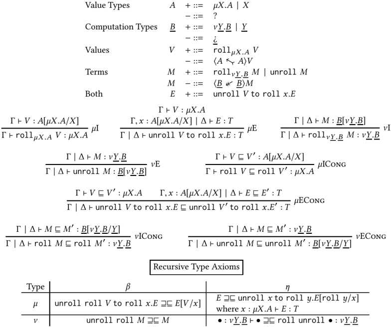CBPV* types, terms, recursive types (diff from GTT), full rules in the extended version <details> <summary>Image 5 Details</summary>  ### Visual Description ## Type System Rules and Axioms ### Overview The image presents a set of type system rules and recursive type axioms, likely related to a programming language or formal system. It defines value types, computation types, values, terms, and expressions, along with inference rules for type checking and axioms for recursive types. ### Components/Axes * **Value Types (A):** Defined recursively as either `μX.A` (a recursive type) or `X` (a type variable). * **Computation Types (B):** Defined recursively as `vY.B` or `Y`. * **Values (V):** Constructed using `roll_{μX.A} V` or `<A ≼ A>V`. * **Terms (M):** Constructed using `roll_{vY.B} M` or `unroll M` or `<B ≼ B>M`. * **Both (E):** `unroll V to roll x.E` * **Judgments:** The rules use judgments of the form `Γ ⊢ V : μX.A`, `Γ, x: A[μX.A/X] | Δ ⊢ E : T`, and `Γ | Δ ⊢ M : vY.B`. * `Γ` and `Δ` are likely type environments or contexts. * `V`, `M`, and `E` represent values, terms, and expressions, respectively. * `A`, `B`, and `T` represent types. * **Inference Rules:** The rules are presented in the standard format: * Premises above the line. * Conclusion below the line. * Rule name on the right. * **Recursive Type Axioms:** A table defining β and η reduction rules for recursive types. ### Detailed Analysis or ### Content Details **Type Definitions:** * `A ::= μX.A | X`: Value types are either recursive types `μX.A` or type variables `X`. * `B ::= vY.B | Y`: Computation types are either recursive types `vY.B` or type variables `Y`. * `V ::= roll_{μX.A} V | <A ≼ A>V`: Values are constructed by rolling a value of type `A` into a recursive type `μX.A` or by `<A ≼ A>V`. * `M ::= roll_{vY.B} M | unroll M | <B ≼ B>M`: Terms are constructed by rolling a term of type `B` into a recursive type `vY.B`, unrolling a term, or by `<B ≼ B>M`. * `E ::= unroll V to roll x.E`: Expressions involve unrolling a value and rolling it back into an expression. **Inference Rules:** 1. **μI (Mu Introduction):** * Premise: `Γ ⊢ V : A[μX.A/X]` * Conclusion: `Γ ⊢ roll_{μX.A} V : μX.A` * Interpretation: If `V` has type `A` where `X` is replaced by `μX.A`, then rolling `V` gives it the recursive type `μX.A`. 2. **μE (Mu Elimination):** * Premise: `Γ, x: A[μX.A/X] | Δ ⊢ E : T` and `Γ ⊢ V : μX.A` * Conclusion: `Γ | Δ ⊢ unroll V to roll x.E : T` * Interpretation: If `E` has type `T` under the assumption that `x` has type `A[μX.A/X]` and `V` has type `μX.A`, then unrolling `V` and rolling it into `E` results in an expression of type `T`. 3. **vI (Nu Introduction):** * Premise: `Γ | Δ ⊢ M : B[vY.B]` * Conclusion: `Γ | Δ ⊢ roll_{vY.B} M : vY.B` * Interpretation: If `M` has type `B` where `Y` is replaced by `vY.B`, then rolling `M` gives it the recursive type `vY.B`. 4. **vE (Nu Elimination):** * Premise: `Γ | Δ ⊢ M : vY.B` * Conclusion: `Γ | Δ ⊢ unroll M : B[vY.B]` * Interpretation: If `M` has type `vY.B`, then unrolling `M` results in a term of type `B[vY.B]`. 5. **μICONG (Mu Congruence):** * Premise: `Γ ⊢ V ≼ V' : A[μX.A/X]` * Conclusion: `Γ ⊢ roll V ≼ roll V' : μX.A` * Interpretation: If `V` is related to `V'` at type `A[μX.A/X]`, then `roll V` is related to `roll V'` at type `μX.A`. 6. **μECON (Mu Expression Congruence):** * Premise: `Γ ⊢ V ≼ V' : μX.A` and `Γ, x: A[μX.A/X] | Δ ⊢ E ≼ E' : T` * Conclusion: `Γ | Δ ⊢ unroll V to roll x.E ≼ unroll V' to roll x.E' : T` * Interpretation: If `V` is related to `V'` at type `μX.A` and `E` is related to `E'` under the assumption that `x` has type `A[μX.A/X]`, then the unrolled and rolled expressions are related at type `T`. 7. **vICONG (Nu Term Congruence):** * Premise: `Γ | Δ ⊢ M ≼ M' : B[vY.B/Y]` * Conclusion: `Γ | Δ ⊢ roll M ≼ roll M' : vY.B` * Interpretation: If `M` is related to `M'` at type `B[vY.B/Y]`, then `roll M` is related to `roll M'` at type `vY.B`. 8. **vECON (Nu Expression Congruence):** * Premise: `Γ | Δ ⊢ M ≼ M' : vY.B` * Conclusion: `Γ | Δ ⊢ unroll M ≼ unroll M' : B[vY.B/Y]` * Interpretation: If `M` is related to `M'` at type `vY.B`, then `unroll M` is related to `unroll M'` at type `B[vY.B/Y]`. **Recursive Type Axioms:** | Type | β | η | | :--- | :---------------------------------------- | :------------------------------------------------------------------------------------------------- | | μ | `unroll roll V to roll x.E ⊐ E[V/x]` | `E ⊐ unroll x to roll y.E[roll y/x]` where `x: μX.A ⊢ E: T` | | v | `unroll roll M ⊐ M` | `: vY.B ⊢ ⊐ roll unroll : vY.B` | * **β-reduction (Beta reduction):** Describes how to simplify expressions involving `unroll` and `roll`. * **η-reduction (Eta reduction):** Describes how to simplify expressions by introducing `unroll` and `roll`. ### Key Observations * The system uses recursive types (`μ` and `v`) to define value and computation types. * The inference rules describe how to type-check expressions involving rolling and unrolling of recursive types. * The axioms provide simplification rules for expressions involving recursive types. ### Interpretation This type system appears to be designed for a language with recursive types and some form of effect or computation type (indicated by `B` and `v`). The `roll` and `unroll` operations are used to introduce and eliminate recursive types, respectively. The inference rules ensure that these operations are type-safe. The axioms provide a way to simplify expressions involving recursive types, which can be useful for program optimization or reasoning about program behavior. The presence of both value types (`A`) and computation types (`B`) suggests a system where values and computations are treated differently, possibly to manage side effects or other computational effects. </details> and ground types G and G are not determined (they were still postulated in Lemma 3.25). For this reason, our translation is parameterized by an interpretation of the dynamic types and the ground casts. By Theorems 3.9, 3.10, we know that these must be embedding-projection pairs (ep pairs), which we now define in CBPV*. There are two kinds of ep pairs we consider: those between value types (where the embedding models an upcast) and those between computation types (where the projection models a downcast). Definition 4.4 (Value and Computation Embedding-Projection Pairs). - (1) A value ep pair from A to A ′ consists of an embedding value x : A /turnstileleft V e : A ′ and projection stack · : FA ′ /turnstileleft S p : FA , satisfying the retraction and projection properties: <!-- formula-not-decoded --> - (2) A computation ep pair from B to B ′ consists of an embedding value z : UB /turnstileleft V e : UB ′ and a projection stack · : B ′ /turnstileleft S p : B satisfying retraction and projection properties: <!-- formula-not-decoded --> While this formulation is very convenient in that both kinds of ep pairs are pairs of a value and a stack, the projection properties are often occur more naturally in the following forms: Lemma 4.5 (Alternative Projection). If ( V e , S p ) is a value ep pair from A to A ′ and Γ , y : A ′ | ∆ /turnstileleft M : B , then <!-- formula-not-decoded --> Similarly, if ( V e , S p ) is a computation ep pair from B to B ′ , and Γ /turnstileleft M : B ′ then <!-- formula-not-decoded --> Proof. For the first, <!-- formula-not-decoded --> For the second, <!-- formula-not-decoded --> Using this, and using the notion of ground type from Section 3.6 with 0 and /latticetop removed , we define Definition 4.6 (Dynamic Type Interpretation). A? , ¿ interpretation ρ consists of (1) a CBPV value type ρ ( ? ) , (2) a CBPV computation type ρ ( ¿ ) , (3) for each value ground type G , a value ep pair ( x . ρ e ( G ) , ρ p ( G )) from /dblbracketleft G /dblbracketright ρ to ρ ( ? ) , and (4) for each computation ground type G , a computation ep pair ( z . ρ e ( G ) , ρ p ( G )) from /dblbracketleft G /dblbracketright ρ to ρ ( ¿ ) . We write /dblbracketleft G /dblbracketright ρ and /dblbracketleft G /dblbracketright ρ for the interpretation of a ground type, replacing ? with ρ ( ? ) , ¿ with ρ ( ¿ ) , and compositionally otherwise. Next, we show several possible interpretations of the dynamic type that will all give, by construction, implementations that satisfy the gradual guarantee. Our interpretations of the value dynamic type are not surprising. They are the usual construction of the dynamic type using type tags: i.e., a recursive sum of basic value types. On the other hand, our interpretations of the computation dynamic type are less familiar. In duality with the interpretation of ?, we interpret ¿ as a recursive product of basic computation types. This interpretation has some analogues in previous work on the duality of computation [Girard 2001; Zeilberger 2009], but the most direct interpretation (definition 4.10) does not correspond to any known work on dynamic/gradual typing. Then we show that a particular choice of which computation types is basic and which are derived produces an interpretation of the dynamic computation type as a type of variable-arity functions whose arguments are passed on the stack, producing a model similar to Scheme without accounting for control effects (definition 4.15). - 4.2.1 Natural Dynamic Type Interpretation. Our first dynamic type interpretation is to make the value and computation dynamic types sums and products of the ground value and computation types, respectively. This forms a model of GTT for the following reasons. For the value dynamic type ?, we need a value embedding (the upcast) from each ground value type G with a corresponding projection. The easiest way to do this would be if for each G , we could rewrite ? as a sum of the values that fit G and those that don't: ? /simequal G + ? -G because of the following lemma. Lemma 4.7 (Sum Injections are Value Embeddings). For any A , A ′ , there are value ep pairs from A and A ′ to A + A ′ where the embeddings are inl and inr . Proof. Define the embedding of A to just be x . inl x and the projection to be bind y ← · ; case y { inl x . ret x | inr . /Omegainv } . This satisfies retraction (using F ( + ) induction (lemma 4.8), inr case is the same): ``` ``` and projection (similarly using F ( + ) induction): ``` ``` Whose proof relies on the following induction principle for the returner type: Lemma 4.8 ( F ( + ) Induction Principle). Γ | · : F ( A 1 + A 2 ) /turnstileleft M 1 /subsetsqequal M 2 : B holds if and only if Γ , V 1 : A 1 /turnstileleft M 1 [ ret inl V 1 ] /subsetsqequal M 2 [ ret inl V 2 ] : B and Γ , V 2 : A 2 /turnstileleft M 2 [ ret inr V 2 ] /subsetsqequal M 2 [ ret inr V 2 ] : B This shows why the type tag interpretation works: it makes the dynamic type in some sense the minimal type with injections from each G : the sum of all value ground types ? /simequal Σ G G . The dynamic computation type ¿ can be naturally defined by a dual construction, by the following dual argument. First, we want a computation ep pair from G to ¿ for each ground computation type G . Specifically, this means we want a stack from ¿ to G (the downcast) with an embedding. The easiest way to get this is if, for each ground computation type G , ¿ is equivalent to a lazy product of G and 'the other behaviors', i.e., ¿ /simequal G & ¿ -G . Then the embedding on π performs the embedded computation, but on π ′ raises a type error. The following lemma, dual to lemma 4.7 shows this forms a computation ep pair: Lemma 4.9 (Lazy Product Projections are Computation Projections). For any B , B ′ , there are computation ep pairs from B and B ′ to B & B ′ where the projections are π and π ′ . Proof. Define the projection for B to be π . Define the embedding by z . { π ↦→ force z | π ′ ↦→ /Omegainv } . Similarly define the projection for B ′ . This satisfies retraction: <!-- formula-not-decoded --> <!-- formula-not-decoded --> <!-- formula-not-decoded --> From this, we see that the easiest way to construct an interpretation of the dynamic computation type is to make it a lazy product of all the ground types G : ¿ /simequal & G G . Using recursive types, we can easily make this a definition of the interpretations: Definition 4.10 (Natural Dynamic Type Interpretation). The following defines a dynamic type interpretation. We define the types to satisfy the isomorphisms <!-- formula-not-decoded --> with the ep pairs defined as in Lemma 4.7 and 4.9. Proof. We can construct ? , ¿ explicitly using recursive and corecursive types. Specifically, we make the recursion explicit by defining open versions of the types: <!-- formula-not-decoded --> Then we define the types ? , ¿ using a standard encoding: <!-- formula-not-decoded --> Then clearly by the roll/unroll isomorphism we get the desired isomorphisms: <!-- formula-not-decoded --> This dynamic type interpretation is a natural fit for CBPV because the introduction forms for ? are exactly the introduction forms for all of the value types (unit, pairing, inl , inr , force ), while elimination forms are all of the elimination forms for computation types ( π , π ′ , application and binding); such 'bityped' languages are related to Girard [2001]; Zeilberger [2009]. Based on this dynamic type interpretation, we can extend GTT to support a truly dynamically typed style of programming, where one can perform case-analysis on the dynamic types at runtime, in addition to the type assertions provided by upcasts and downcasts. Theaxioms we choose might seem to under-specify the dynamic type, but because of the uniqueness of adjoints, the following are derivable. and projection: <!-- formula-not-decoded --> Fig. 7. Natural Dynamic Type Extension of GTT Lemma 4.11 (Natural Dynamic Type Extension Theorems). The following are derivable in GTT with the natural dynamic type extension <!-- formula-not-decoded --> We explore this in more detail with the next dynamic type interpretation. Next, we easily see that if we want to limit GTT to just the CBV types (i.e. the only computation types are A → FA ′ ), then we can restrict the dynamic types as follows: Definition 4.12 (CBV Dynamic Type Interpretation). The following is a dynamic type interpretation for the ground types of GTT with only function computation types: <!-- formula-not-decoded --> And finally if we restrict GTT to only CBN types (i.e., the only value type is booleans 1 + 1), we can restrict the dynamic types as follows: Definition 4.13 (CBN Dynamic Type Interpretation). The following is a dynamic type interpretation for the ground types of GTT with only boolean value types: <!-- formula-not-decoded --> 4.2.2 Scheme-like Dynamic Type Interpretation. The above dynamic type interpretation does not correspond to any dynamically typed language used in practice, in part because it includes explicit cases for the 'additives', the sum type + and lazy product type &. Normally, these are not included in this way, but rather sums are encoded by making each case use a fresh constructor (using nominal techniques like opaque structs in Racket) and then making the sum the union of the constructors, as argued in Siek and Tobin-Hochstadt [2016]. We leave modeling this nominal structure to future work, but in minimalist languages, such as simple dialects of Scheme and Lisp, sum types are often encoded structurally rather than nominally by using some fixed sum type of symbols , also called atoms . Then a value of a sum type is modeled by a pair of a symbol (to indicate the case) and a payload with the actual value. We can model this by using the canonical isomorphisms <!-- formula-not-decoded --> and representing sums as pairs, and lazy products as functions. The fact that isomorphisms are ep pairs is useful for constructing the ep pairs needed in the dynamic type interpretation. Lemma 4.14 (Isomorphisms are EP Pairs). If x : A /turnstileleft V ′ : A ′ and x ′ : A ′ /turnstileleft V : A are an isomorphism in that V [ V ′ / x ′ ] /supersetsqequal /subsetsqequal x and V [ V / x ] /supersetsqequal /subsetsqequal x ′ , then ( x . V ′ , bind x ′ ← · ; ret V ′ ) are a value ep pair from A to A ′ . Similarly if · : B /turnstileleft S ′ : B ′ and · : B ′ /turnstileleft S : B are an isomorphism in that S [ S ′ ] ≡ · and S ′ [ S ] ≡ · then ( z . S ′ [ force z ] , S ) is an ep pair from B to B ′ . With this in mind, we remove the cases for sums and lazy pairs from the natural dynamic types, and include some atomic type as a case of ?-for simplicity we will just use booleans. We also do not need a case for 1, because we can identify it with one of the booleans, say true . This leads to the following definition: Definition 4.15 (Scheme-like Dynamic Type Interpretation). We can define a dynamic type interpretation with the following type isomorphisms: <!-- formula-not-decoded --> Proof. We construct ? , ¿ explicitly as follows. First define X : val type /turnstileleft Tree [ X ] val type to be the type of binary trees: <!-- formula-not-decoded --> Next, define X : val type , Y : ctype /turnstileleft VarArg [ X , Y ] comp type to be the type of variable-arity functions from X to Y : <!-- formula-not-decoded --> Then we define an open version of ? , ¿ with respect to a variable representing the occurrences of ? in ¿: <!-- formula-not-decoded --> <!-- formula-not-decoded --> Then we can define the closed versions using a recursive type: <!-- formula-not-decoded --> The ep pairs for × , U , F , → are clear. To define the rest, first note that there is an ep pair from 1 + 1 to ? by Lemma 4.7. Next, we can define 1 to be the ep pair to 1 + 1 defined by the left case and Lemma 4.7, composed with this. The ep pair for ? + ? is defined by composing the isomorphism (which is always an ep pair) ( ? + ? ) /simequal (( 1 + 1 )× ? ) with the ep pair for 1 + 1 using the action of product types on ep pairs (proven as part of Theorem 4.23): ( ? + ? ) /simequal (( 1 + 1 )× ? ) /triangleleft ( ? × ? ) /triangleleft ? (where we write A /triangleleft A ′ to mean there is an ep pair from A to A ′ ). Similarly, for ¿ & ¿, we use action of the function type on ep pairs (also proven as part of Theorem 4.23): ¿ & ¿ /simequal (( 1 + 1 ) → ¿ ) /triangleleft ( ? → ¿ ) /triangleleft ¿ /square If we factor out some of the recursion to use inductive and coinductive types, we get the following isomorphisms: <!-- formula-not-decoded --> That is a dynamically typed value is a binary tree whose leaves are either booleans or closures. We think of this as a simple type of S-expressions. A dynamically typed computation is a variablearity function that is called with some number of dynamically typed value arguments ? and returns a dynamically typed result F ?. This captures precisely the function type of Scheme, which allows for variable arity functions! What's least clear is why the type <!-- formula-not-decoded --> Should be thought of as a type of variable arity functions. First consider the infinite unrolling of this type: <!-- formula-not-decoded --> this says that a term of type VarArg [ X ][ Y ] offers an infinite number of possible behaviors: it can act as a function from X n → Y for any n . Similarly in Scheme, a function can be called with any number of arguments. Finally note that this type is isomorphic to a function that takes a cons-list of arguments: <!-- formula-not-decoded --> But operationally the type VarArg [ ? ][ F ? ] is a more faithful model of Scheme implementations because all of the arguments are passed individually on the stack, whereas the type ( µX . 1 + ( ? × X )) → FX is a function that takes a single argument that is a list. These two are distinguished in Scheme and the 'dot args' notation witnesses the isomorphism. Based on this dynamic type interpretation we can make a 'Scheme-like' extension to GTT in Figure 8. First, we add a boolean type B with true , false and if-then-else. Next, we add in the elimination form for ? and the introduction form for ¿. The elimination form for ? is a typed version of Scheme's match macro. The introduction form for ¿ is a typed, CBPV version of Scheme's caselambda construct. Finally, we add type dynamism rules expressing the representations of 1, A + A , and A × A in terms of booleans that were explicit in the ep pairs used in Definition 4.15. The reader may be surprised by how few axioms we need to add to GTT for this extension: for instance we only define the upcast from 1 to B and not vice-versa, and similarly the sum/lazy pair type isomorphisms only have one cast defined when a priori there are 4 to be defined. Finally for the dynamic types we define β and η laws that use the ground casts as injections and projections respectively, but we don't define the corresponding dual casts (the ones that possibly error). <!-- formula-not-decoded --> Fig. 8. Scheme-like Extension to GTT In fact all of these expected axioms can be proven from those we have shown. Again we see the surprising rigidity of GTT: because an F downcast is determined by its dual value upcast (and vice-versa for U upcasts), we only need to define the upcast as long as the downcast could be implemented already. Because we give the dynamic types the universal property of a sum/lazy product type respectively, we can derive the implementations of the 'checking' casts. All of the proofs are direct from the uniqueness of adjoints lemma. Theorem 4.16 (Boolean to Unit Downcast). In Scheme-like GTT, we can prove <!-- formula-not-decoded --> Theorem 4.17 (Tagged Value to Sum). In Scheme-like GTT, we can prove <!-- formula-not-decoded --> and the downcasts are given by lemma 4.14. Theorem 4.18 (Lazy Product to Tag Checking Function). In Scheme-like GTT, we can prove <!-- formula-not-decoded --> and the upcasts are given by lemma 4.14. Theorem 4.19 (Ground Mismatches are Errors). In Scheme-like GTT we can prove ``` ``` Finally, we note now that all of these axioms are satisfied when using the Scheme-like dynamic type interpretation and extending the translation of GTT into CBPV* with the following, tediously explicit definition: ``` ``` ## 4.3 Contract Translation Having defined the data parameterizing the translation, we now consider the translation of GTT into CBPV* itself. For the remainder of the paper, we assume that we have a fixed dynamic type interpretation ρ , and all proofs and definitions work for any interpretation. - 4.3.1 Interpreting Casts as Contracts. The main idea of the translation is an extension of the dynamic type interpretation to an interpretation of all casts in GTT (Figure 9) as contracts in CBPV*, following the definitions in Lemma 3.25. Some clauses of the translation are overlapping, which we resolve by considering them as ordered (though we will ultimately show they are equivalent). The definition is also not obviously total: we need to verify that it covers every possible case where A /subsetsqequal A ′ and B /subsetsqequal B ′ . To prove totality and coherence, we could try induction on the type dynamism relation of Figure 2, but it is convenient to first give an alternative, normalized set of rules for type dynamism that proves the same relations, which we do in Figure 10. Lemma 4.20 (Normalized Type Dynamism is E/q.sc\_u.scivalent to Original). T /subsetsqequal T ′ is provable in the normalized typed dynamism definition iff it is provable in the original typed dynamism definition. Proof. It is clear that the normalized system is a subset of the original: every normalized rule corresponds directly to a rule of the original system, except the normalized A /subsetsqequal ? and B /subsetsqequal ¿ rules have a subderivation that was not present originally. For the converse, first we show by induction that reflexivity is admissible: - (1) If A ∈ { ? , 1 , 0 } , we use a normalized rule. Fig. 9. 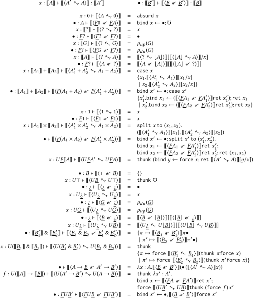Cast to Contract Translation <details> <summary>Image 6 Details</summary>  ### Visual Description ## Mathematical Expressions and Code Snippets ### Overview The image contains a collection of mathematical expressions and code snippets, likely related to functional programming or type theory. The expressions involve symbols, functions, and data structures, presented in a formal notation. ### Components/Axes The image is divided into two columns of expressions. Each expression typically consists of a variable assignment (e.g., `x: ... = ...`) or a function definition (e.g., `f: ... = ...`). The expressions use symbols like `[[ ]]`, `+`, `×`, `→`, `&`, and various Greek letters. There are also keywords like `absurd`, `bind`, `case`, `split`, `thunk`, `force`, and `ret`. ### Detailed Analysis or Content Details Here's a transcription of the expressions, organized by column: **Left Column:** 1. `x: [[A]] + [[(A' ⋈ A)]] : [[A']]` 2. `x: 0 ⊢ [[(A ⋈ 0)]] = absurd x` 3. `•: A ⊢ [[(F0 ⋈ FA)]] = bind x ← •; U` 4. `x: [[?]] ⊢ [[(<? ⋈ ?>)]] = x` 5. `•: F? ⊢ [[(F? ⋈ F?)]] = ρup(G)` 6. `x: [[G]] ⊢ [[(<? ⋈ G)]] = ρdn(G)` 7. `•: F? ⊢ [[(FG ⋈ F?)]] = [[<? ⊢ [[A]] ⊢ [[(<? ⋈ A)]] = [[<A ⊢ [[A]] ⊢ [[(<? ⋈ ?>)]]/x]` 8. `: F? ⊢ [[(A ⋈ ?)]] = case x` 9. `x: [[A1]] + [[A2]] ⊢ [[(A'1 + A'2 ⋈ A1 + A2)]] = {x1.[[(A'1 ⋈ A1)]][x1/x] | x2.[[(A'2 ⋈ A2)]][x2/x]}` 10. `: [[A1]] + [[A2]] ⊢ [[(F(A1 + A2) ⋈ F(A'1 + A'2))]] = bind x' ← •; case x' {x'1.bind x1 ← [[(FA1 ⋈ FA'1)]]ret x'1; ret x1 | x'2.bind x2 ← [[(FA2 ⋈ FA'2)]]ret x'2; ret x2}` 11. `x: 1 ⊢ [[(1 ⋈ 1)]] = x` 12. `: F1 ⊢ [[(F1 ⋈ F1)]] = split x to (x1, x2).` 13. `x: [[A1]] × [[A2]] ⊢ [[(A'1 × A'2 ⋈ A1 × A2)]] = ([[(A'1 ⋈ A1)]][x1], [[(A'2 ⋈ A2)]][x2])` 14. `⊢ [[(F(A1 × A2) ⋈ F(A'1 × A'2))]] = bind x' ← •; split x' to (x'1, x'2). bind x1 ← [[(FA1 ⋈ FA'1)]]ret x'1; bind x2 ← [[(FA2 ⋈ FA'2)]]ret x'2; ret (x1, x2)` 15. `x: UF[[A]] ⊢ [[(UFA' ⋈ UFA)]] = thunk (bind y ← force x; ret [[(A' ⋈ A)]][y/x])` 16. `: B ⊢ [[(T ⋈ B)]] = {}` 17. `x: UT ⊢ [[(UB ⋈ UT)]] = thunk U` 18. `: ¿ ⊢ [[(¿ ⋈ ¿)]] = •` 19. `x: U¿ ⊢ [[(U¿ ⋈ U¿)]] = x` 20. `: ¿ ⊢ [[(G ⋈ ¿)]] = ρdn(G)` 21. `x: UG ⊢ [[(U¿ ⋈ UG)]] = ρup(G)` 22. `: ¿ ⊢ [[(B ⋈ ¿)]] = [[B ⋈ |B]]` 23. `x: U¿ ⊢ [[(U¿ ⋈ UB)]] = [[U¿ ⋈ U[B]] ⊢ [[(U[B] ⋈ UB)]]` 24. `•: [[B'1]] & [[B'2]] ⊢ [[(B1 & B2 ⋈ B'1 & B'2)]] = {π ⊢ [[(B1 ⋈ B'1)]]π. | π' ⊢ [[(B2 ⋈ B'2)]]π'•}` 25. `x: U([[B1]] & [[B2]]) ⊢ [[(U(B'1 & B'2) ⋈ U(B1 & B2))]] = thunk {π ⊢ force [[(B'1 ⋈ B1)]] (thunk π force x) | π' ⊢ force [[(B'2 ⋈ B2)]] (thunk π'force x)}` 26. `f: U([[A]] → [[B]]) ⊢ [[(U(A' → B') ⋈ U(A → B))]] = λx: A.[[B ⋈ B']](([[A' ⋈ A]]x))` 27. `: FUB' ⊢ [[(FUB ⋈ FUB')]] = thunk λx': A'. bind x ← [[(FA ⋈ FA')]]ret x'; force [[(UB' ⋈ UB)]] thunk (force f) x'` 28. `: FUB' ⊢ [[(FUB ⋈ FUB')]] = bind x' ← •; [[(B ⋈ B')]] force x'` **Right Column:** 1. `•: [[B' ⋈ B]] ⊢ [[(B ⋈ B')]] : [[B]]` ### Key Observations * The expressions use a combination of mathematical notation and programming constructs. * The `⋈` symbol seems to represent some kind of relation or operation between terms. * The `⊢` symbol likely represents a type assignment or a logical entailment. * The `[[ ]]` notation might represent a semantic interpretation or a type environment. * The code snippets involve concepts like binding, case analysis, and thunking, which are common in functional programming. ### Interpretation The image likely presents a formal system for reasoning about types and programs. The expressions define rules for type checking, evaluation, or transformation of programs. The system seems to involve concepts from type theory, logic, and functional programming. The specific meaning of the symbols and expressions would require more context or a formal definition of the system. </details> - (2) If A /nelement { ? , 1 , 0 } , we use the inductive hypothesis and the monotonicity rule. - (3) If B ∈ { ¿ , /latticetop } use the normalized rule. - (4) If B /nelement { ¿ , /latticetop } use the inductive hypothesis and monotonicity rule. Next, we show that transitivity is admissible: Fig. 10. Normalized Type Dynamism Relation | A ∈ { ? , 1 } | A ∈ { ? , 0 } | A /subsetsqequal /floorleft A /floorright A /nelement { 0 , ? } | |------------------------|-----------------------------------------------------|---------------------------------------------------------------------------------------------| | A /subsetsqequal A | 0 /subsetsqequal A | A /subsetsqequal ? | | B /subsetsqequal B ′ | A 1 /subsetsqequal A ′ 1 A 2 /subsetsqequal A ′ 2 | A 1 /subsetsqequal A ′ 1 A 2 /subsetsqequal A ′ 2 | | UB /subsetsqequal UB ′ | A 1 + A 2 /subsetsqequal A ′ 1 + A ′ 2 | A 1 × A 2 /subsetsqequal A ′ 1 × A ′ 2 | | ¿ /subsetsqequal ¿ | B ∈ { ¿ , /latticetop} /latticetop /subsetsqequal B | B /subsetsqequal /floorleft B /floorright B /nelement {/latticetop , ¿ } B /subsetsqequal ¿ | | A /subsetsqequal A ′ | B 1 /subsetsqequal B ′ 1 B 2 /subsetsqequal B ′ 2 | A /subsetsqequal A ′ B /subsetsqequal B ′ | | FA /subsetsqequal FA ′ | B 1 & B 2 /subsetsqequal B ′ 1 & B ′ 2 | A → B /subsetsqequal A ′ → B ′ | - (1) Assume we have A /subsetsqequal A ′ /subsetsqequal A ′′ 2. (a) If the left rule is 0 /subsetsqequal A ′ , then either A ′ = ? or A ′ = 0. If A ′ = 0 the right rule is 0 /subsetsqequal A ′′ and we can use that proof. Otherwise, A ′ = ? then the right rule is ? /subsetsqequal ? and we can use 0 /subsetsqequal ?. 3. (b) If the left rule is A /subsetsqequal A where A ∈ { ? , 1 } then either A = ?, in which case A ′′ = ? and we're done. Otherwise the right rule is either 1 /subsetsqequal 1 (done) or 1 /subsetsqequal ? (also done). 4. (c) If the left rule is A /subsetsqequal ? with A /nelement { 0 , ? } then the right rule must be ? /subsetsqequal ? and we're done. 5. (d) Otherwise the left rule is a monotonicity rule for one of U , + , × and the right rule is either monotonicity (use the inductive hypothesis) or the right rule is A ′ /subsetsqequal ? with a sub-proof of A ′ /subsetsqequal /floorleft A ′ /floorright . Since the left rule is monotonicity, /floorleft A /floorright = /floorleft A ′ /floorright , so we inductively use transitivity of the proof of A /subsetsqequal A ′ with the proof of A ′ /subsetsqequal /floorleft A ′ /floorright to get a proof A /subsetsqequal /floorleft A /floorright and thus A /subsetsqequal ?. - (2) Assume we have B /subsetsqequal B ′ /subsetsqequal B ′′ . 7. (a) If the left rule is /latticetop /subsetsqequal B ′ then B ′′ ∈ { ¿ , /latticetop } so we apply that rule. 8. (b) If the left rule is ¿ /subsetsqequal ¿, the right rule must be as well. 9. (c) If the left rule is B /subsetsqequal ¿ the right rule must be reflexivity. 10. (d) If the left rule is a monotonicity rule for & , → , F then the right rule is either also monotonicity (use the inductive hypothesis) or it's a B /subsetsqequal ¿ rule and we proceed with ? above Finally we show A /subsetsqequal ?, B /subsetsqequal ¿ are admissible by induction on A , B . - (1) If A ∈ { ? , 0 } we use the primitive rule. - (2) If A /nelement { ? , 0 } we use the A /subsetsqequal ? rule and we need to show A /subsetsqequal /floorleft A /floorright . If A = 1, we use the 1 /subsetsqequal 1 rule, otherwise we use the inductive hypothesis and monotonicity. - (3) If B ∈ { ¿ , /latticetop } we use the primitive rule. - (4) If B /nelement { ¿ , /latticetop } we use the B /subsetsqequal ¿ rule and we need to show B /subsetsqequal /floorleft B /floorright , which follows by inductive hypothesis and monotonicity. Every other rule in Figure 2 is a rule of the normalized system in Figure 10. Based on normalized type dynamism, we show Theorem 4.21. If A /subsetsqequal A ′ according to Figure 10, then there is a unique complex value x : A /turnstileleft /dblbracketleft 〈 A ′ /arrowtailleft A 〉 /dblbracketright x : A ′ and if B /subsetsqequal B ′ according to Figure 10, then there is a unique complex stack x : B /turnstileleft /dblbracketleft 〈 B ′ /arrowtailleft B 〉 /dblbracketright x : B ′ /square - 4.3.2 Interpretation of Terms. Next, we extend the translation of casts to a translation of all terms by congruence, since all terms in GTT besides casts are in CBPV*. This satisfies: Lemma 4.22 (Contract Translation Type Preservation). If Γ | ∆ /turnstileleft E : T in GTT, then /dblbracketleft Γ /dblbracketright | /dblbracketleft ∆ /dblbracketright /turnstileleft /dblbracketleft E /dblbracketright : /dblbracketleft T /dblbracketright in CBPV*. - 4.3.3 Interpretation of Term Dynamism. We have now given an interpretation of the types, terms, and type dynamism proofs of GTT in CBPV*. To complete this to form a model of GTT, we need to give an interpretation of the term dynamism proofs, which is established by the following 'axiomatic graduality' theorem. GTT has heterogeneous term dynamism rules indexed by type dynamism, but CBPV* has only homogeneous inequalities between terms, i.e., if E /subsetsqequal E ′ , then E , E ′ have the same context and types. Since every type dynamism judgement has an associated contract, we can translate a heterogeneous term dynamism to a homogeneous inequality up to contract . Our next overall goal is to prove Theorem 4.23 (Axiomatic Graduality). For any dynamic type interpretation, <!-- formula-not-decoded --> where we define /dblbracketleft Φ /dblbracketright to upcast each variable, and /dblbracketleft ∆ /dblbracketright to downcast · if it is nonempty, and if ∆ = · , then M [ /dblbracketleft ∆ /dblbracketright ] = M . More explicitly, - (1) If Φ : Γ /subsetsqequal Γ ′ , then there exists n such that Γ = x 1 : A 1 , . . . , x n : A n and Γ ′ = x ′ 1 : A ′ 1 , . . . , x ′ n : A ′ n where A i /subsetsqequal A ′ i for each i ≤ n . Then /dblbracketleft Φ /dblbracketright is a substitution from /dblbracketleft Γ /dblbracketright to /dblbracketleft Γ ′ /dblbracketright defined as <!-- formula-not-decoded --> - (2) If Ψ : ∆ /subsetsqequal ∆ ′ , then we similarly define /dblbracketleft Ψ /dblbracketright as a 'linear substitution'. That is, if ∆ = ∆ ′ = · , then /dblbracketleft Ψ /dblbracketright is an empty substitution and M [ /dblbracketleft Ψ /dblbracketright ] = M , otherwise /dblbracketleft Ψ /dblbracketright is a linear substitution from ∆ ′ = · : B ′ to ∆ = · : B where B /subsetsqequal B ′ defined as <!-- formula-not-decoded --> Relative to previous work on graduality [New and Ahmed 2018], the distinction between complex value upcasts and complex stack downcasts guides the formulation of the theorem; e.g. using upcasts in the left-hand theorem would require more thunks/forces. We now develop some lemmas on the way towards proving this result. First, to keep proofs high-level, we establish the following cast reductions that follow easily from β , η principles. Lemma 4.24 (Cast Reductions). The following are all provable ``` ``` Our next goal is to show that from the basic casts being ep pairs, we can prove that all casts as defined in Figure 9 are ep pairs. Before doing so, we prove the following lemma, which is used for transitivity (e.g. in the A /subsetsqequal ? rule, which uses a composition A /subsetsqequal /floorleft A /floorright /subsetsqequal ?): ## Lemma 4.25 (EP Pairs Compose). - (1) If ( V 1 , S 1 ) is a value ep pair from A 1 to A 2 and ( V 2 , S 2 ) is a value ep pair from A 2 to A 3 , then ( V 2 [ V 1 ] , S 1 [ S 2 ]) is a value ep pair from A 1 to A 3 . - (2) If ( V 1 , S 1 ) is a computation ep pair from B 1 to B 2 and ( V 2 , S 2 ) is a computation ep pair from B 2 to B 3 , then ( V 2 [ V 1 ] , S 1 [ S 2 ]) is a computation ep pair from B 1 to B 3 . Proof. (1) First, retraction follows from retraction twice: <!-- formula-not-decoded --> and projection follows from projection twice: <!-- formula-not-decoded --> ``` ``` - (2) Again retraction follows from retraction twice: ``` ``` and projection from projection twice: ``` ``` Lemma 4.26 (Identity EP Pair). ( x . x , ·) is an ep pair (value or computation). Now, we show that all casts are ep pairs. The proof is a somewhat tedious, but straightforward calculation. Lemma 4.27 (Casts are EP Pairs). - (1) For any A /subsetsqequal A ′ , the casts ( x . /dblbracketleft 〈 A ′ /arrowtailleft A 〉 x /dblbracketright , /dblbracketleft 〈 FA /dblarrowheadleft FA ′ 〉 /dblbracketright ) are a value ep pair from /dblbracketleft A /dblbracketright to /dblbracketleft A ′ /dblbracketright - (2) For any B /subsetsqequal B ′ , the casts ( z . /dblbracketleft 〈 UB ′ /arrowtailleft UB 〉 z /dblbracketright , /dblbracketleft 〈 B /dblarrowheadleft B ′ 〉 /dblbracketright ) are a computation ep pair from /dblbracketleft B /dblbracketright to /dblbracketleft B ′ /dblbracketright . Proof. By induction on normalized type dynamism derivations. - (1) A /subsetsqequal A ( A ∈ { ? , 1 } ), because identity is an ep pair. - (2) 0 /subsetsqequal A (that A ∈ { ? , 0 } is not important): 3. (a) Retraction is ``` ``` which holds by 0 η - (b) Projection is ``` ``` Which we calculate: ``` ``` ## (a) Retraction is ``` ``` ``` ``` ``` ``` ## (a) First, Retraction: ``` ``` ## (b) Next, Projection: <!-- formula-not-decoded --> (5) U : By inductive hypothesis, ( x . /dblbracketleft 〈 UB ′ /arrowtailleft UB 〉 /dblbracketright , 〈 B /dblarrowheadleft B ′ 〉) is a computation ep pair - (a) To show retraction we need to prove: x : UB /turnstileleft ret x /supersetsqequal /subsetsqequal bind y ←( ret thunk /dblbracketleft 〈 UB ′ /arrowtailleft UB 〉 /dblbracketright ) ; ret thunk /dblbracketleft 〈 B /dblarrowheadleft B ′ 〉 /dblbracketright [ force y ] : FUB ′ Which we calculate as follows: <!-- formula-not-decoded --> - (b) To show projection we calculate: <!-- formula-not-decoded --> - (1) There's a few base cases about the dynamic computation type, then - (2) /latticetop : 3. (a) Retraction is by /latticetop η : 4. (b) Projection is - (3) &: 6. (a) Retraction <!-- formula-not-decoded --> <!-- formula-not-decoded --> <!-- formula-not-decoded --> ``` ``` ## (b) Projection ``` ``` - (5) F : (a) To show retraction we need to show ``` ``` We calculate: <!-- formula-not-decoded --> - (b) To show projection we need to show <!-- formula-not-decoded --> We calculate as follows <!-- formula-not-decoded --> While the above was tedious, this pays off greatly in later proofs: this is the only proof in the entire development that needs to inspect the definition of a 'shifted' cast (a downcast between F types or an upcast between U types). All later lemmas have cases for these shifted casts, but only use the property that they are part of an ep pair. This is one of the biggest advantages of using an explicit syntax for complex values and complex stacks: the shifted casts are the only ones that non-trivially use effectful terms, so after this lemma is established we only have to manipulate values and stacks, which compose much more nicely than effectful terms. Conceptually, the main reason we can avoid reasoning about the definitions of the shifted casts directly is that any two shifted casts that form an ep pair with the same value embedding/stack projection are equal: Lemma 4.28 (Value Embedding determines Projection, Computation Projection determines Embedding). For any value x : A /turnstileleft V e : A ′ and stacks · : FA ′ /turnstileleft S 1 : FA and · : FA ′ /turnstileleft S 2 : FA , if ( V e , S 1 ) and ( V e , S 2 ) are both value ep pairs, then <!-- formula-not-decoded --> Similarly for any values x : UB /turnstileleft V 1 : UB ′ and x : UB /turnstileleft V 2 : UB ′ and stack · : B ′ /turnstileleft S p : B , if ( V 1 , S p ) and ( V 2 , S p ) are both computation ep pairs then <!-- formula-not-decoded --> Proof. By symmetry it is sufficient to show S 1 /subsetsqequal S 2 . S 1 /subsetsqequal S 1 | bind x ← S 1 ; ret x /subsetsqequal bind x ←• ; S 1 [ ret x ] | |-----------------------------------------------------------------| | bind x ← S 1 ; ret V e /subsetsqequal bind x ←• ; ret x | | bind x ← S 1 ; ret x /subsetsqequal bind x ←• ; S 2 [ ret x ] | <!-- formula-not-decoded --> similarly to show V 1 /subsetsqequal V 2 : <!-- formula-not-decoded --> /square The next two lemmas on the way to axiomatic graduality show that Figure 9 translates 〈 A /arrowtailleft A 〉 to the identity and 〈 A ′′ /arrowtailleft A ′ 〉〈 A ′ /arrowtailleft A 〉 to the same contract as 〈 A ′′ /arrowtailleft A 〉 , and similarly for downcasts. Intuitively, for all connectives except F , U , this is because of functoriality of the type constructors on values and stacks. For the F , U cases, we will use the corresponding fact about the dual cast, i.e., to prove the FA to FA downcast is the identity stack, we know by inductive hypothesis that the A to A upcast is the identity, and that the identity stack is a projection for the identity. Therefore Lemma 4.28 implies that the FA downcast must be equivalent to the identity. We now discuss these two lemmas and their proofs in detail. First, we show that the casts from a type to itself are equivalent to the identity. Below, we will use this lemma to prove the reflexivity case of the axiomatic graduality theorem, and to prove a conservativity result, which says that a GTT homogeneous term dynamism is the same as a CBPV* inequality between their translations. Lemma 4.29 (Identity Expansion). For any A and B , <!-- formula-not-decoded --> Proof. Weproceed by induction on A , B , following the proof that reflexivity is admissible given in Lemma 4.20. - (1) If A ∈ { 1 , ? } , then /dblbracketleft 〈 A /arrowtailleft A 〉 /dblbracketright [ x ] = x . - (2) If A = 0, then absurd x /supersetsqequal /subsetsqequal x by 0 η . - (3) If A = UB , then by inductive hypothesis /dblbracketleft 〈 B /dblarrowheadleft B 〉 /dblbracketright /supersetsqequal /subsetsqequal · . By Lemma 4.26, ( x . x , ·) is a computation ep pair from B to itself. But by Lemma 4.27, ( /dblbracketleft 〈 UB /arrowtailleft UB 〉 /dblbracketright [ x ] , ·) is also a computation ep pair so the result follows by uniqueness of embeddings from computation projections Lemma 4.28. - (4) If A = A 1 × A 2 or A = A 1 + A 2, the result follows by the η principle and inductive hypothesis. - (5) If B = ¿, /dblbracketleft 〈 ¿ /dblarrowheadleft ¿ 〉 /dblbracketright = · . - (6) For B = /latticetop , the result follows by /latticetop η . - (7) For B = B 1 & B 2 or B = A → B ′ , the result follows by inductive hypothesis and η . - (8) For B = FA , by inductive hypothesis, the downcast is a projection for the value embedding x . x , so the result follows by identity ep pair and uniqueness of projections from value embeddings. /square Second, we show that a composition of upcasts is translated to the same thing as a direct upcast, and similarly for downcasts. Below, we will use this lemma to translate transitivity of term dynamism in GTT. Lemma 4.30 (Cast Decomposition). For any dynamic type interpretation ρ , <!-- formula-not-decoded --> Proof. By mutual induction on A , B . - (1) A /subsetsqequal A ′ /subsetsqequal A ′′ 2. (a) If A = 0, we need to show x : 0 /turnstileleft /dblbracketleft 〈 A ′′ /arrowtailleft 0 〉 /dblbracketright [ x ] /supersetsqequal /subsetsqequal /dblbracketleft 〈 A ′′ /arrowtailleft A ′ 〉 /dblbracketright [ /dblbracketleft 〈 A ′ /arrowtailleft 0 〉 /dblbracketright [ x ]] : A ′′ which follows by 0 η . 3. (b) If A = ?, then A ′ = A ′′ = ?, and both casts are the identity. 4. (c) If A /nelement { ? , 0 } and A ′ = ?, then A ′′ = ? and /dblbracketleft 〈 ? /arrowtailleft ? 〉 /dblbracketright [ /dblbracketleft 〈 ? /arrowtailleft A 〉 /dblbracketright ] = /dblbracketleft 〈 ? /arrowtailleft A 〉 /dblbracketright by definition. 5. (d) If A , A ′ /nelement { ? , 0 } and A ′′ = ?, then /floorleft A /floorright = /floorleft A ′ /floorright , which we call G and <!-- formula-not-decoded --> and <!-- formula-not-decoded --> so this reduces to the case for A /subsetsqequal A ′ /subsetsqequal G , below. - (e) If A , A ′ , A ′′ /nelement { ? , 0 } , then they all have the same top-level constructor: - (i) + : We need to show for A 1 /subsetsqequal A ′ 1 /subsetsqequal A ′′ 1 and A 2 /subsetsqequal A ′ 2 /subsetsqequal A ′′ 2 : x : /dblbracketleft A 1 /dblbracketright + /dblbracketleft A 2 /dblbracketright /turnstileleft /dblbracketleft 〈 A ′′ 1 + A ′′ 2 /arrowtailleft A ′ 1 + A ′ 2 〉 /dblbracketright [ /dblbracketleft 〈 A ′ 1 + A ′ 2 /arrowtailleft A 1 + A 2 〉 /dblbracketright [ x ]] /supersetsqequal/subsetsqequal /dblbracketleft 〈 A ′′ 1 + A ′′ 2 /arrowtailleft A 1 + A 2 〉 /dblbracketright [ x ] : /dblbracketleft A We proceed as follows: <!-- formula-not-decoded --> <!-- formula-not-decoded --> - (ii) 1: By definition both sides are the identity. - (iii) × : We need to show for A 1 /subsetsqequal A ′ 1 /subsetsqequal A ′′ 1 and A 2 /subsetsqequal A ′ 2 /subsetsqequal A ′′ 2 : x : /dblbracketleft A 1 /dblbracketright × /dblbracketleft A 2 /dblbracketright /turnstileleft /dblbracketleft 〈 A ′′ 1 × A ′′ 2 /arrowtailleft A ′ 1 × A ′ 2 〉 /dblbracketright [ /dblbracketleft 〈 A ′ 1 × A ′ 2 /arrowtailleft A 1 × A 2 〉 /dblbracketright [ x ]] /supersetsqequal/subsetsqequal /dblbracketleft 〈 A ′′ 1 × A ′′ 2 /arrowtailleft A 1 × A 2 〉 /dblbracketright [ x ] : /dblbracketleft A We proceed as follows: <!-- formula-not-decoded --> - (iv) UB /subsetsqequal UB ′ /subsetsqequal UB ′′ . We need to show <!-- formula-not-decoded --> By composition of ep pairs, we know ( x . /dblbracketleft 〈 UB ′′ /arrowtailleft UB ′ 〉 /dblbracketright [ /dblbracketleft 〈 UB ′ /arrowtailleft UB 〉 /dblbracketright [ x ]] , /dblbracketleft 〈 B /dblarrowheadleft B ′ 〉 /dblbracketright [ /dblbracketleft 〈 B ′ /dblarrowheadleft B ′′ 〉 /dblbracketright ]) is a computation ep pair. Furthermore, by inductive hypothesis, we know <!-- formula-not-decoded --> so then both sides form ep pairs paired with /dblbracketleft 〈 B /dblarrowheadleft B ′′ 〉 /dblbracketright , so it follows because computation projections determine embeddings 4.28. ## (2) B /subsetsqequal B ′ /subsetsqequal B ′′ - (a) If B = /latticetop , then the result is immediate by η /latticetop . - (b) If B = ¿, then B ′ = B ′′ = ¿ then both sides are just · . - (c) If B /nelement { ¿ , /latticetop } , and B ′ = ¿, then B ′′ = ¿ <!-- formula-not-decoded --> - (d) If B , B ′ /nelement { ¿ , /latticetop } , and B ′′ = ¿ , and /floorleft B /floorright = /floorleft B ′ /floorright , which we call G . Then we need to show <!-- formula-not-decoded --> so the result follows from the case B /subsetsqequal B ′ /subsetsqequal G , which is handled below. - (e) If B , B ′ , B ′′ /nelement { ¿ , /latticetop } , then they all have the same top-level constructor: - (i) & We are given B 1 /subsetsqequal B ′ 1 /subsetsqequal B ′′ 1 and B 2 /subsetsqequal B ′ 2 /subsetsqequal B ′′ 2 and we need to show <!-- formula-not-decoded --> <!-- formula-not-decoded --> - (ii) → , assume we are given A /subsetsqequal A ′ /subsetsqequal A ′′ and B /subsetsqequal B ′ /subsetsqequal B ′′ , then we proceed: <!-- formula-not-decoded --> - (iii) FA /subsetsqequal FA ′ /subsetsqequal FA ′′ . First, by composition of ep pairs, we know <!-- formula-not-decoded --> form a value ep pair. Furthermore, by inductive hypothesis, we know <!-- formula-not-decoded --> so the two sides of our equation are both projections with the same value embedding, so the equation follows from uniqueness of projections from value embeddings. /square The final lemma before the graduality theorem lets us 'move a cast' from left to right or viceversa, via the adjunction property for ep pairs. These arise in the proof cases for return and thunk , because in those cases the inductive hypothesis is in terms of an upcast (downcast) and the conclusion is in terms of a a downcast (upcast). Lemma 4.31 (Hom-set formulation of Adjunction). For any value embedding-projection pair V e , S p from A to A ′ , the following are equivalent: <!-- formula-not-decoded --> For any computation ep pair ( V e , S p ) from B to B ′ , the following are equivalent: <!-- formula-not-decoded --> - Proof. (1) Assume ret V e [ V ] /subsetsqequal M : FA ′ . Then by retraction, ret V /subsetsqequal S p [ ret V e [ V ]] so by transitivity, the result follows by substitution: <!-- formula-not-decoded --> - (2) Assume ret V /subsetsqequal S p [ M ] : FA . Then by projection, bind x ← S p [ M ] ; ret V e [ x ] /subsetsqequal M , so it is sufficient to show <!-- formula-not-decoded --> but again by substitution we have <!-- formula-not-decoded --> and by Fβ , the LHS is equivalent to ret V e [ V ] . - (3) Assume z ′ : UB ′ /turnstileleft M /subsetsqequal S [ S p [ force z ′ ]] , then by projection, S [ S p [ force V e ]] /subsetsqequal S [ force z ] and by substitution: <!-- formula-not-decoded --> - (4) Assume z : UB /turnstileleft M [ V e / z ′ ] /subsetsqequal S [ force z ] . Then by retraction, M /subsetsqequal M [ V e [ thunk S p [ force z ]]] and by substitution: <!-- formula-not-decoded --> and the right is equivalent to S [ S p [ force z ]] by Uβ . /square Finally, we prove the axiomatic graduality theorem. In addition to the lemmas above, the main task is to prove the 'compatibility' cases which are the congruence cases for introduction and elimination rules. These come down to proving that the casts 'commute' with introduction/elimination forms, and are all simple calculations. Theorem(AxiomaticGraduality). For any dynamic type interpretation, the following are true: <!-- formula-not-decoded --> Proof. By mutual induction over term dynamism derivations. For the β , η and reflexivity rules, we use the identity expansion lemma and the corresponding β , η rule of CBPV*4.29. For compatibility rules a pattern emerges. Universal rules (positive intro, negative elim) are easy, wedon't need to reason about casts at all. For '(co)-pattern matching rules' (positive elim, negative intro), we need to invoke the η principle (or commuting conversion, which is derived from the η principle). In all compatibility cases, the cast reduction lemma keeps the proof straightforward. Fortunately, all reasoning about 'shifted' casts is handled in lemmas, and here we only deal with the 'nice' value upcasts/stack downcasts. - (1) Transitivity for values: The GTT rule is <!-- formula-not-decoded --> Which under translation (and the same assumptions about the contexts) is <!-- formula-not-decoded --> We proceed as follows, the key lemma here is the cast decomposition lemma: <!-- formula-not-decoded --> - (2) Transitivity for terms: The GTT rule is <!-- formula-not-decoded --> Which under translation (and the same assumptions about the contexts) is <!-- formula-not-decoded --> We proceed as follows, the key lemma here is the cast decomposition lemma: <!-- formula-not-decoded --> - (3) Substitution of a value in a value: The GTT rule is <!-- formula-not-decoded --> Where Φ : Γ /subsetsqequal Γ ′ . Under translation, we need to show <!-- formula-not-decoded --> Which follows by compositionality: <!-- formula-not-decoded --> - (4) Substitution of a value in a term: The GTT rule is <!-- formula-not-decoded --> Where Φ : Γ /subsetsqequal Γ ′ and Ψ : ∆ /subsetsqequal ∆ ′ . Under translation this is: /dblbracketleft Γ /dblbracketright , x : /dblbracketleft A /dblbracketright | /dblbracketleft ∆ /dblbracketright /turnstileleft /dblbracketleft M /dblbracketright /subsetsqequal /dblbracketleft 〈 B /dblarrowheadleft B ′ 〉 /dblbracketright [ /dblbracketleft M ′ /dblbracketright [ /dblbracketleft Φ /dblbracketright ][ /dblbracketleft 〈 A ′ /arrowtailleft A 〉 /dblbracketright [ x ]/ x ′ ]] : /dblbracketleft B /dblbracketright /dblbracketleft Γ /dblbracketright /turnstileleft /dblbracketleft 〈 A ′ /arrowtailleft A 〉 /dblbracketright [ /dblbracketleft V /dblbracketright ] /subsetsqequal /dblbracketleft V ′ /dblbracketright [ /dblbracketleft Φ /dblbracketright ] : /dblbracketleft A ′ /dblbracketright /dblbracketleft Γ /dblbracketright | /dblbracketleft ∆ /dblbracketright /turnstileleft /dblbracketleft M [ V / x ] /dblbracketright /subsetsqequal /dblbracketleft 〈 B /dblarrowheadleft B ′ 〉 /dblbracketright [ /dblbracketleft M ′ [ V ′ / x ′ ] /dblbracketright [ /dblbracketleft Φ /dblbracketright ]] : /dblbracketleft B /dblbracketright Which follows from compositionality of the translation: <!-- formula-not-decoded --> - (5) Substitution of a term in a stack: The GTT rule is <!-- formula-not-decoded --> Where Φ : Γ /subsetsqequal Γ ′ . Under translation this is <!-- formula-not-decoded --> We follows easily using compositionality of the translation: <!-- formula-not-decoded --> - (6) Variables: The GTT rule is <!-- formula-not-decoded --> which under translation is <!-- formula-not-decoded --> which is an instance of reflexivity. - (7) Hole: The GTT rule is <!-- formula-not-decoded --> which under translation is <!-- formula-not-decoded --> which is an instance of reflexivity. - (8) Error is bottom: The GTT axiom is <!-- formula-not-decoded --> where Φ : Γ /subsetsqequal Γ ′ , so we need to show <!-- formula-not-decoded --> which is an instance of the error is bottom axiom of CBPV. - (9) Error strictness: The GTT axiom is <!-- formula-not-decoded --> where Φ : Γ /subsetsqequal Γ ′ , which under translation is <!-- formula-not-decoded --> <!-- formula-not-decoded --> By strictness of stacks in CBPV, both sides are equivalent to /Omegainv , so it follows by reflexivity. (10) UpCast-L: The GTT axiom is <!-- formula-not-decoded --> which under translation is <!-- formula-not-decoded --> Which follows by identity expansion and reflexivity. - (11) UpCast-R: The GTT axiom is <!-- formula-not-decoded --> which under translation is <!-- formula-not-decoded --> which follows by identity expansion and reflexivity. - (12) DnCast-R: The GTT axiom is <!-- formula-not-decoded --> Which under translation is <!-- formula-not-decoded --> Which follows by identity expansion and reflexivity. - (13) DnCast-L: The GTT axiom is <!-- formula-not-decoded --> So under translation we need to show <!-- formula-not-decoded --> Which follows immediately by reflexivity and the lemma that identity casts are identities. (14) 0 elim, we do the term case, the value case is similar <!-- formula-not-decoded --> Immediate by 0 η . - (15) + intro, we do the inl case, the inr case is the same: <!-- formula-not-decoded --> Which follows easily: <!-- formula-not-decoded --> <!-- formula-not-decoded --> - (16) + elim, we do just the cases where the continuations are terms: <!-- formula-not-decoded --> case /dblbracketleft V /dblbracketright { x 1 . /dblbracketleft M 1 /dblbracketright [ /dblbracketleft Ψ /dblbracketright ] | x 2 . /dblbracketleft M 2 /dblbracketright [ /dblbracketleft Ψ /dblbracketright ]} /subsetsqequal /dblbracketleft 〈 B /dblarrowheadleft B ′ 〉 /dblbracketright [ case /dblbracketleft V /dblbracketright ′ [ /dblbracketleft Φ /dblbracketright ]{ x ′ 1 . /dblbracketleft M ′ 1 /dblbracketright [ /dblbracketleft Φ /dblbracketright ] | x ′ 2 . /dblbracketleft M ′ 2 /dblbracketright [ /dblbracketleft Φ /dblbracketright ]}] case /dblbracketleft V /dblbracketright { x 1 . /dblbracketleft M 1 /dblbracketright [ /dblbracketleft Ψ /dblbracketright ] | x 2 . /dblbracketleft M 2 /dblbracketright [ /dblbracketleft Ψ /dblbracketright ]} /subsetsqequal /dblbracketleft 〈 B /dblarrowheadleft B ′ 〉 /dblbracketright [ case /dblbracketleft V /dblbracketright { x 1 . /dblbracketleft M ′ 1 /dblbracketright [ /dblbracketleft Φ /dblbracketright ][ /dblbracketleft 〈 A ′ 1 /arrowtailleft A 1 〉 /dblbracketright [ x 1 ]/ x ′ 1 ] | x 2 . /dblbracketleft M ′ 2 /dblbracketright [ /dblbracketleft Φ /dblbracketright ][ /dblbracketleft 〈 A ′ 2 /arrowtailleft A 2 〉 /dblbracketright [ x 2 ]/ x ′ 2 ]}] (IH) /supersetsqequal /subsetsqequal case /dblbracketleft V /dblbracketright (comm conv) { x 1 . /dblbracketleft 〈 B /dblarrowheadleft B ′ 〉 /dblbracketright [ /dblbracketleft M ′ 1 /dblbracketright [ /dblbracketleft Φ /dblbracketright ][ /dblbracketleft 〈 A ′ 1 /arrowtailleft A 1 〉 /dblbracketright [ x 1 ]/ x ′ 1 ]] | x 2 . /dblbracketleft 〈 B /dblarrowheadleft B ′ 〉 /dblbracketright [ /dblbracketleft M ′ 2 /dblbracketright [ /dblbracketleft Φ /dblbracketright ][ /dblbracketleft 〈 A ′ 2 /arrowtailleft A 2 〉 /dblbracketright [ x 2 ]/ x ′ 2 ]]} /supersetsqequal /subsetsqequal case /dblbracketleft V /dblbracketright ( + β ) { x 1 . /dblbracketleft 〈 B /dblarrowheadleft B ′ 〉 /dblbracketright [ case inl /dblbracketleft 〈 A ′ 1 /arrowtailleft A 1 〉 /dblbracketright x 1 { x ′ 1 . /dblbracketleft M ′ 1 /dblbracketright [ /dblbracketleft Φ /dblbracketright ] | x ′ 2 . /dblbracketleft M ′ 2 /dblbracketright [ /dblbracketleft Φ /dblbracketright ]}] | x 2 . /dblbracketleft 〈 B /dblarrowheadleft B ′ 〉 /dblbracketright [ case inr /dblbracketleft 〈 A ′ 2 /arrowtailleft A 2 〉 /dblbracketright x 2 { x ′ 1 . /dblbracketleft M ′ 1 /dblbracketright [ /dblbracketleft Φ /dblbracketright ] | x ′ 2 . /dblbracketleft M ′ 2 /dblbracketright [ /dblbracketleft Φ /dblbracketright ]}]} /supersetsqequal /subsetsqequal case /dblbracketleft V /dblbracketright (cast reduction) { x 1 . /dblbracketleft 〈 B /dblarrowheadleft B ′ 〉 /dblbracketright [ case /dblbracketleft 〈 A ′ 1 + A ′ 2 /arrowtailleft A 1 + A 2 〉 /dblbracketright inl x 1 { x ′ 1 . /dblbracketleft M ′ 1 /dblbracketright [ /dblbracketleft Φ /dblbracketright ] | x ′ 2 . /dblbracketleft M ′ 2 /dblbracketright [ /dblbracketleft Φ /dblbracketright ]}] | x 2 . /dblbracketleft 〈 B /dblarrowheadleft B ′ 〉 /dblbracketright [ case /dblbracketleft 〈 A ′ 1 + A ′ 2 /arrowtailleft A 1 + A 2 〉 /dblbracketright inr x 2 { x ′ 1 . /dblbracketleft M ′ 1 /dblbracketright [ /dblbracketleft Φ /dblbracketright ] | x ′ 2 . /dblbracketleft M ′ 2 /dblbracketright [ /dblbracketleft Φ /dblbracketright ]}]} /supersetsqequal /subsetsqequal /dblbracketleft 〈 B /dblarrowheadleft B ′ 〉 /dblbracketright [ case /dblbracketleft 〈 A ′ 1 + A ′ 2 /arrowtailleft A 1 + A 2 〉 /dblbracketright [ /dblbracketleft V /dblbracketright ]{ x ′ 1 . /dblbracketleft M ′ 1 /dblbracketright [ /dblbracketleft Φ /dblbracketright ] | x ′ 2 . /dblbracketleft M ′ 2 /dblbracketright [ /dblbracketleft Φ /dblbracketright ]}] /subsetsqequal /dblbracketleft 〈 B /dblarrowheadleft B ′ 〉 /dblbracketright [ case /dblbracketleft V ′ /dblbracketright [ /dblbracketleft Φ /dblbracketright ]{ x ′ 1 . /dblbracketleft M ′ 1 /dblbracketright [ /dblbracketleft Φ /dblbracketright ] | x ′ 2 . /dblbracketleft M ′ 2 /dblbracketright [ /dblbracketleft Φ /dblbracketright ]}] (IH) - (17) 1 intro: <!-- formula-not-decoded --> Immediate by cast reduction. - (18) 1 elim (continuations are terms case): <!-- formula-not-decoded --> which follows by identity expansion 4.29. - (19) × intro: ## /dblbracketleft 〈 A ′ 1 /arrowtailleft A 1 〉 /dblbracketright/dblbracketleft V 1 /dblbracketright /subsetsqequal /dblbracketleft V ′ 1 [ /dblbracketleft Φ /dblbracketright ] /dblbracketright /dblbracketleft 〈 A ′ 2 /arrowtailleft A 2 〉 /dblbracketright/dblbracketleft V 2 /dblbracketright /subsetsqequal /dblbracketleft V ′ 2 [ /dblbracketleft Φ /dblbracketright ] /dblbracketright /dblbracketleft 〈 A ′ 1 × A ′ 2 /arrowtailleft A 1 × A 2 〉 /dblbracketright [( /dblbracketleft V 1 /dblbracketright , /dblbracketleft V 2 /dblbracketright )] /subsetsqequal ( /dblbracketleft V ′ 1 [ /dblbracketleft Φ /dblbracketright ] /dblbracketright , /dblbracketleft V ′ 2 [ /dblbracketleft Φ /dblbracketright ] /dblbracketright ) We proceed: /dblbracketleft 〈 A ′ 1 × A ′ 2 /arrowtailleft A 1 × A 2 〉 /dblbracketright [( /dblbracketleft V 1 /dblbracketright , /dblbracketleft V 2 /dblbracketright )] /supersetsqequal/subsetsqequal ( /dblbracketleft 〈 A ′ 1 /arrowtailleft A 1 〉 /dblbracketright/dblbracketleft V 1 /dblbracketright , /dblbracketleft 〈 A ′ 2 /arrowtailleft A 2 〉 /dblbracketright/dblbracketleft V 2 /dblbracketright ) (cast reduction) <!-- formula-not-decoded --> ## /subsetsqequal ( /dblbracketleft V 1 [ /dblbracketleft Φ /dblbracketright ] /dblbracketright , /dblbracketleft V 2 [ /dblbracketleft Φ /dblbracketright ] /dblbracketright - (20) × elim: We show the case where the continuations are terms, the value continuations are no different: <!-- formula-not-decoded --> We proceed as follows: split /dblbracketleft V /dblbracketright to ( x , y ) . /dblbracketleft M /dblbracketright [ /dblbracketleft Ψ /dblbracketright ] /subsetsqequal split /dblbracketleft V /dblbracketright to ( x , y ) . /dblbracketleft 〈 B /dblarrowheadleft B ′ 〉 /dblbracketright [ /dblbracketleft M ′ /dblbracketright [ /dblbracketleft Φ /dblbracketright ][ /dblbracketleft 〈 A ′ ]] (IH) <!-- formula-not-decoded --> <!-- formula-not-decoded --> /supersetsqequal /subsetsqequal (cast reduction) split /dblbracketleft V /dblbracketright to ( x , y ) . <!-- formula-not-decoded --> <!-- formula-not-decoded --> /supersetsqequal /subsetsqequal /dblbracketleft 〈 B /dblarrowheadleft (21) U intro: <!-- formula-not-decoded --> We proceed as follows: <!-- formula-not-decoded --> (22) U elim: B ′ 〉 /dblbracketright [ split /dblbracketleft V ′ /dblbracketright [ /dblbracketleft Φ /dblbracketright ] to ( x ′ , y ′ ) . /dblbracketleft M ′ /dblbracketright [ /dblbracketleft Φ /dblbracketright ]] (commuting conversion) /arrowtailleft <!-- formula-not-decoded --> A 〉 /dblbracketright [ x ]/ x <!-- formula-not-decoded --> By hom-set formulation of adjunction 4.31. (23) /latticetop intro: Immediate by /latticetop η (24) & intro: <!-- formula-not-decoded --> We proceed as follows: <!-- formula-not-decoded --> (25) & elim, we show the π case, π ′ is symmetric: <!-- formula-not-decoded --> ′ ][ /dblbracketleft 〈 A ′ /arrowtailleft A 〉 /dblbracketright [ y ]/ y ′ (26) We proceed as follows: <!-- formula-not-decoded --> <!-- formula-not-decoded --> We proceed as follows: λx : A . /dblbracketleft M /dblbracketright [ /dblbracketleft Ψ /dblbracketright ] /subsetsqequal λx : A . /dblbracketleft 〈 B /dblarrowheadleft B ′ 〉 /dblbracketright [ /dblbracketleft M ′ /dblbracketright [ /dblbracketleft Φ /dblbracketright ][ /dblbracketleft 〈 A ′ /arrowtailleft A 〉 /dblbracketright x / x ′ ]] (IH) /supersetsqequal /subsetsqequal λx : A . ( /dblbracketleft 〈 A → B /dblarrowheadleft A ′ → B ′ 〉 /dblbracketright [ λx ′ . /dblbracketleft M ′ /dblbracketright [ /dblbracketleft Φ /dblbracketright ]]) x (cast reduction) /supersetsqequal /subsetsqequal /dblbracketleft 〈 A → B /dblarrowheadleft A ′ → B ′ 〉 /dblbracketright [ λx ′ . /dblbracketleft M ′ /dblbracketright [ /dblbracketleft Φ /dblbracketright ]] ( → η ) - (27) We need to show <!-- formula-not-decoded --> We proceed: ## /dblbracketleft M /dblbracketright [ /dblbracketleft Ψ /dblbracketright ] /dblbracketleft V /dblbracketright <!-- formula-not-decoded --> - (28) We need to show <!-- formula-not-decoded --> By hom-set definition of adjunction 4.31 - (29) We need to show ## /dblbracketleft M /dblbracketright [ /dblbracketleft Ψ /dblbracketright ] /subsetsqequal /dblbracketleft 〈 FA /dblarrowheadleft FA ′ 〉 /dblbracketright [ /dblbracketleft M ′ /dblbracketright [ Φ ]] /dblbracketleft N /dblbracketright /subsetsqequal /dblbracketleft 〈 B /dblarrowheadleft B ′ 〉 /dblbracketright [ /dblbracketleft N /dblbracketright [ Φ ][ /dblbracketleft 〈 A ′ /arrowtailleft A 〉 /dblbracketright x / x ′ ]] bind x ← /dblbracketleft M /dblbracketright [ /dblbracketleft Ψ /dblbracketright ] ; /dblbracketleft N /dblbracketright /subsetsqequal /dblbracketleft 〈 B /dblarrowheadleft B ′ 〉 /dblbracketright [ bind x ′ ← /dblbracketleft M ′ /dblbracketright [ /dblbracketleft Φ /dblbracketright ] ; /dblbracketleft N ′ /dblbracketright [ /dblbracketleft Φ /dblbracketright ]] We proceed: bind x ← /dblbracketleft M /dblbracketright [ /dblbracketleft Ψ /dblbracketright ] ; /dblbracketleft N /dblbracketright /subsetsqequal bind x ← /dblbracketleft 〈 FA /dblarrowheadleft FA ′ 〉 /dblbracketright [ /dblbracketleft M ′ /dblbracketright [ Φ ]] ; /dblbracketleft 〈 B /dblarrowheadleft B ′ 〉 /dblbracketright [ /dblbracketleft N /dblbracketright [ Φ ][ /dblbracketleft 〈 A ′ /arrowtailleft A 〉 /dblbracketright x / x ′ ]] (IH, congruence) /supersetsqequal /subsetsqequal bind x ← /dblbracketleft 〈 FA /dblarrowheadleft FA ′ 〉 /dblbracketright [ /dblbracketleft M ′ /dblbracketright [ Φ ]] ; bind x ′ ← ret /dblbracketleft 〈 A ′ /arrowtailleft A 〉 /dblbracketright [ x ] ; /dblbracketleft 〈 B /dblarrowheadleft B ′ 〉 /dblbracketright [ /dblbracketleft N /dblbracketright [ Φ ]] ( Fβ ) /subsetsqequal bind x ′ ← /dblbracketleft M ′ /dblbracketright [ Φ ] ; /dblbracketleft 〈 B /dblarrowheadleft B ′ 〉 /dblbracketright [ /dblbracketleft N /dblbracketright [ Φ ]] (Projection) /supersetsqequal /subsetsqequal /dblbracketleft 〈 B /dblarrowheadleft B ′ 〉 /dblbracketright [ bind x ′ ← /dblbracketleft M ′ /dblbracketright [ Φ ] ; /dblbracketleft N /dblbracketright [ Φ ]] (commuting conversion) /square ``` ``` Fig. 11. Operational CBPV Syntax As a corollary, we have the following conservativity result, which says that the homogeneous term dynamisms in GTT are sound and complete for inequalities in CBPV*. Corollary 4.32 (Conservativity). If Γ | ∆ /turnstileleft E , E ′ : T are two terms of the same type in the intersection of GTT and CBPV*, then Γ | ∆ /turnstileleft E /subsetsqequal E ′ : T is provable in GTT iff it is provable in CBPV*. Proof. The reverse direction holds because CBPV* is a syntactic subset of GTT. The forward direction holds by axiomatic graduality and the fact that identity casts are identities. /square ## 5 COMPLEX VALUE/STACK ELIMINATION Next, to bridge the gap between the semantic notion of complex value and stack with the more rigid operational notion, we perform a complexity-elimination pass. This translates a computation with complex values in it to an equivalent computation without complex values: i.e., all pattern matches take place in computations, rather than in values, and translates a term dynamism derivation that uses complex stacks to one that uses only 'simple' stacks without pattern-matching and computation introduction forms. Stacks do not appear anywhere in the grammar of terms, but they are used in the equational theory (computation η rules and error strictness). This translation clarifies the behavioral meaning of complex values and stacks, following Munch-Maccagnoni [2014]; Führmann [1999], and therefore of upcasts and downcasts. This is related to completeness of focusing: it moves inversion rules outside of focus phases. The syntax of operational CBPV is as in Figure 1 (unshaded), but with recursive types added as in Section 4.1, and with values and stacks restricted as in Figure 11. In CBPV, values include only introduction forms, as usual for values in operational semantics, and CBPV stacks consist only of elimination forms for computation types (the syntax of CBPV enforces an A-normal form, where only values can be pattern-matched on, so case and split are not evaluation contexts in the operational semantics). Levy [2003] translates CBPV* to CBPV, but not does not prove the inequality preservation that we require here, so we give an alternative translation for which this property is easy to verify . We translate both complex values and complex stacks to fully general computations, so that computation pattern-matching can replace the pattern-matching in complex values/stacks. For example, for a closed value, we could 'evaluate away' the complexity and get a closed simple value (if we don't use U ), but for open terms, evaluation will get 'stuck' if we pattern match on a variable-so not every complex value can be translated to a value in CBPV.More formally, we translate a CBPV* complex value V : A to a CBPV computation V † : FA that in CBPV* is equivalent to ret V . Similarly, we translate a CBPV* complex stack S with hole · : B to a CBPV computation S † with a free variable z : UB such that in CBPV*, S † /supersetsqequal /subsetsqequal S [ force z ] . Computations M : B are translated to computations M † with the same type. Fig. 12. 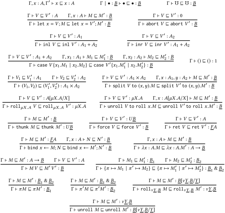CBPV Inequational Theory (Congruence Rules) <details> <summary>Image 7 Details</summary>  ### Visual Description ## Type Theory Rules: Judgement Derivations ### Overview The image presents a collection of type theory inference rules, likely related to a formal system for programming languages or logic. Each rule defines how to derive a judgement (a statement about types and terms) from other judgements. The rules cover various constructs, including variables, functions, products, sums, recursive types, and control flow. ### Components/Axes The image consists of multiple inference rules. Each rule has the following structure: * **Premises:** Judgements above the horizontal line. These are the conditions that must be satisfied to apply the rule. * **Conclusion:** The judgement below the horizontal line. This is the judgement that can be derived if the premises are satisfied. * **Context (Γ):** A set of assumptions about the types of variables. * **Terms (M, N, V):** Expressions in the language. * **Types (A, B):** Classifications of terms. * **Judgements:** Statements of the form "Γ ⊢ M : A", meaning "in context Γ, term M has type A". * **Other Symbols:** Various symbols representing type constructors, term constructors, and operations (e.g., × for product types, + for sum types, μ for recursive types). ### Detailed Analysis or ### Content Details Here's a breakdown of each rule, transcribing the text and explaining its meaning: 1. **Variable Rule:** * `Γ, x: A, Γ' ⊢ x : A` * Meaning: If variable `x` has type `A` in the context, then `x` has type `A`. 2. **Unit Type Introduction:** * `Γ ⊢ • : B` * `Γ ⊢ • ⊏ • : B` * Meaning: The unit value `•` has type `B`. 3. **Union Type Introduction:** * `Γ ⊢ ∪ ⊏ ∪ : B` * Meaning: The union value `∪` has type `B`. 4. **Let Binding:** * `Γ ⊢ V ⊏ V' : A Γ, x: A ⊢ M ⊏ M' : B` * `Γ ⊢ let x = V; M ⊏ let x = V'; M': B` * Meaning: If `V` has type `A` and `M` has type `B` assuming `x` has type `A`, then `let x = V; M` has type `B`. 5. **Abort Rule:** * `Γ ⊢ V ⊏ V' : 0` * `Γ ⊢ abort V ⊏ abort V': B` * Meaning: If `V` has type `0` (empty type), then `abort V` has type `B`. 6. **Inl (Left Injection):** * `Γ ⊢ V ⊏ V' : A1` * `Γ ⊢ inl V ⊏ inl V': A1 + A2` * Meaning: If `V` has type `A1`, then `inl V` has type `A1 + A2` (sum type). 7. **Inr (Right Injection):** * `Γ ⊢ V ⊏ V' : A2` * `Γ ⊢ inr V ⊏ inr V': A1 + A2` * Meaning: If `V` has type `A2`, then `inr V` has type `A1 + A2` (sum type). 8. **Unit Value:** * `Γ ⊢ () ⊏ () : 1` * Meaning: The unit value `()` has type `1`. 9. **Case Analysis:** * `Γ ⊢ V ⊏ V' : A1 + A2 Γ, x1: A1 ⊢ M1 ⊏ M1' : B Γ, x2: A2 ⊢ M2 ⊏ M2' : B` * `Γ ⊢ case V {x1.M1 | x2.M2} ⊏ case V' {x1.M1' | x2.M2'}: B` * Meaning: If `V` has type `A1 + A2`, `M1` has type `B` assuming `x1` has type `A1`, and `M2` has type `B` assuming `x2` has type `A2`, then the case expression has type `B`. 10. **Pair Formation:** * `Γ ⊢ V1 ⊏ V1' : A1 Γ ⊢ V2 ⊏ V2' : A2` * `Γ ⊢ (V1, V2) ⊏ (V1', V2'): A1 × A2` * Meaning: If `V1` has type `A1` and `V2` has type `A2`, then the pair `(V1, V2)` has type `A1 × A2` (product type). 11. **Split (Pair Decomposition):** * `Γ ⊢ V ⊏ V' : A1 × A2 Γ, x: A1, y: A2 ⊢ M ⊏ M' : B` * `Γ ⊢ split V to (x, y).M ⊏ split V' to (x, y).M': B` * Meaning: If `V` has type `A1 × A2` and `M` has type `B` assuming `x` has type `A1` and `y` has type `A2`, then the split expression has type `B`. 12. **Roll (Recursive Type Introduction):** * `Γ ⊢ V ⊏ V' : A[μX.A/X]` * `Γ ⊢ rollμX.A V ⊏ rollμX.A V': μX.A` * Meaning: If `V` has type `A[μX.A/X]` (A with `μX.A` substituted for `X`), then `rollμX.A V` has type `μX.A` (recursive type). 13. **Unroll (Recursive Type Elimination):** * `Γ ⊢ V ⊏ V' : μX.A Γ, x: A[μX.A/X] ⊢ M ⊏ M' : B` * `Γ ⊢ unroll V to roll x.M ⊏ unroll V' to roll x.M': B` * Meaning: If `V` has type `μX.A` and `M` has type `B` assuming `x` has type `A[μX.A/X]`, then the unroll expression has type `B`. 14. **Thunk (Suspension):** * `Γ ⊢ M ⊏ M' : B` * `Γ ⊢ thunk M ⊏ thunk M': UB` * Meaning: If `M` has type `B`, then `thunk M` has type `UB` (suspended computation). 15. **Force (Evaluation of Suspension):** * `Γ ⊢ V ⊏ V' : UB` * `Γ ⊢ force V ⊏ force V': B` * Meaning: If `V` has type `UB`, then `force V` has type `B`. 16. **Return (Value):** * `Γ ⊢ M ⊏ M' : FA` * `Γ ⊢ ret V ⊏ ret V': A` * Meaning: If `M` has type `FA`, then `ret V` has type `A`. 17. **Bind (Monadic Binding):** * `Γ ⊢ M ⊏ M' : FA Γ, x: A ⊢ N ⊏ N' : B` * `Γ ⊢ bind x ← M; N ⊏ bind x ← M'; N': B` * Meaning: If `M` has type `FA` and `N` has type `B` assuming `x` has type `A`, then the bind expression has type `B`. 18. **Lambda Abstraction:** * `Γ, x: A ⊢ M ⊏ M' : B` * `Γ ⊢ λx: A.M ⊏ λx: A.M': A → B` * Meaning: If `M` has type `B` assuming `x` has type `A`, then `λx: A.M` has type `A → B` (function type). 19. **Application:** * `Γ ⊢ M ⊏ M' : A → B Γ ⊢ V ⊏ V' : A` * `Γ ⊢ MV ⊏ M'V': B` * Meaning: If `M` has type `A → B` and `V` has type `A`, then `MV` has type `B`. 20. **Record Update:** * `Γ ⊢ M1 ⊏ M1' : B1 Γ ⊢ M2 ⊏ M2' : B2` * `Γ ⊢ {π ← M1 | π' → M2} ⊏ {π ← M1' | π' → M2'}: B1 & B2` * Meaning: If `M1` has type `B1` and `M2` has type `B2`, then the record update expression has type `B1 & B2`. 21. **And Type Introduction (Left Projection):** * `Γ ⊢ M ⊏ M' : B1 & B2` * `Γ ⊢ πM ⊏ πM': B1` * Meaning: If `M` has type `B1 & B2` (product type), then `πM` (left projection) has type `B1`. 22. **And Type Introduction (Right Projection):** * `Γ ⊢ M ⊏ M' : B1 & B2` * `Γ ⊢ π'M ⊏ π'M': B2` * Meaning: If `M` has type `B1 & B2` (product type), then `π'M` (right projection) has type `B2`. 23. **Roll with Variable:** * `Γ ⊢ M ⊏ M' : B[vY.B/Y]` * `Γ ⊢ rollvY.B M ⊏ rollvY.B M': vY.B` * Meaning: If `M` has type `B[vY.B/Y]`, then `rollvY.B M` has type `vY.B`. 24. **Unroll with Variable:** * `Γ ⊢ M ⊏ M' : vY.B` * `Γ ⊢ unroll M ⊏ unroll M': B[vY.B/Y]` * Meaning: If `M` has type `vY.B`, then `unroll M` has type `B[vY.B/Y]`. ### Key Observations * The rules define a type system with features like sum types, product types, recursive types, and monadic effects. * The rules use a judgement form `Γ ⊢ M ⊏ M' : A`, which suggests a relation between two terms `M` and `M'` of type `A` in context `Γ`. This could represent a form of subtyping, refinement typing, or program equivalence. * The presence of `UB` and `FA` types, along with `thunk`, `force`, `ret`, and `bind` rules, indicates the presence of monadic effects, likely for handling side effects or control flow. * The rules for `roll` and `unroll` define recursive types, allowing for the definition of self-referential data structures. ### Interpretation The image presents a formal type system that likely underpins a programming language or logical framework. The rules define how to assign types to terms and how to derive new judgements from existing ones. The system includes features for handling data structures (products, sums, recursive types), control flow (monads), and potentially program equivalence or refinement. The specific meaning of the `⊏` relation would need further context to fully understand, but it likely plays a crucial role in the system's semantics. The rules are essential for ensuring type safety and reasoning about the behavior of programs within this system. </details> | Γ , x : A , Γ ′ /turnstileleft x /subsetsqequal x : A Γ | • : B /turnstileleft • /subsetsqequal • : B | Γ , x : A , Γ ′ /turnstileleft x /subsetsqequal x : A Γ | • : B /turnstileleft • /subsetsqequal • : B | Γ , x : A , Γ ′ /turnstileleft x /subsetsqequal x : A Γ | • : B /turnstileleft • /subsetsqequal • : B | Γ , x : A , Γ ′ /turnstileleft x /subsetsqequal x : A Γ | • : B /turnstileleft • /subsetsqequal • : B | Γ , x : A , Γ ′ /turnstileleft x /subsetsqequal x : A Γ | • : B /turnstileleft • /subsetsqequal • : B | Γ , x : A , Γ ′ /turnstileleft x /subsetsqequal x : A Γ | • : B /turnstileleft • /subsetsqequal • : B | Γ , x : A , Γ ′ /turnstileleft x /subsetsqequal x : A Γ | • : B /turnstileleft • /subsetsqequal • : B | Γ /turnstileleft /Omegainv /subsetsqequal /Omegainv : B | |--------------------------------------------------------------------------------------------------------------|--------------------------------------------------------------------------------------------------------------|--------------------------------------------------------------------------------------------------------------|--------------------------------------------------------------------------------------------------------------|--------------------------------------------------------------------------------------------------------------|--------------------------------------------------------------------------------------------------------------|--------------------------------------------------------------------------------------------------------------|-------------------------------------------------------------------------------------------------------------| | Γ /turnstileleft V /subsetsqequal V ′ : A Γ , x : A /turnstileleft M /subsetsqequal M ′ : B | Γ /turnstileleft V /subsetsqequal V ′ : A Γ , x : A /turnstileleft M /subsetsqequal M ′ : B | Γ /turnstileleft V /subsetsqequal V ′ : A Γ , x : A /turnstileleft M /subsetsqequal M ′ : B | Γ /turnstileleft V /subsetsqequal V ′ : A Γ , x : A /turnstileleft M /subsetsqequal M ′ : B | Γ /turnstileleft V /subsetsqequal V ′ : A Γ , x : A /turnstileleft M /subsetsqequal M ′ : B | Γ /turnstileleft V /subsetsqequal V ′ : A Γ , x : A /turnstileleft M /subsetsqequal M ′ : B | Γ /turnstileleft V /subsetsqequal V ′ : 0 | Γ /turnstileleft V /subsetsqequal V ′ : 0 | | Γ /turnstileleft let x = V ; M /subsetsqequal let x = V ′ ; M ′ : B | Γ /turnstileleft let x = V ; M /subsetsqequal let x = V ′ ; M ′ : B | Γ /turnstileleft let x = V ; M /subsetsqequal let x = V ′ ; M ′ : B | Γ /turnstileleft let x = V ; M /subsetsqequal let x = V ′ ; M ′ : B | Γ /turnstileleft let x = V ; M /subsetsqequal let x = V ′ ; M ′ : B | Γ /turnstileleft let x = V ; M /subsetsqequal let x = V ′ ; M ′ : B | Γ /turnstileleft abort V /subsetsqequal abort V ′ : B | Γ /turnstileleft abort V /subsetsqequal abort V ′ : B | | Γ /turnstileleft V /subsetsqequal V ′ : A 1 | Γ /turnstileleft V /subsetsqequal V ′ : A 1 | Γ /turnstileleft V /subsetsqequal V ′ : A 1 | Γ /turnstileleft V /subsetsqequal V ′ : A 1 | Γ /turnstileleft V /subsetsqequal V ′ : A 1 | Γ /turnstileleft V /subsetsqequal V ′ : A 1 | Γ /turnstileleft V /subsetsqequal V ′ : A 2 | Γ /turnstileleft V /subsetsqequal V ′ : A 2 | | Γ /turnstileleft inl V /subsetsqequal inl V ′ : A 1 + A 2 | Γ /turnstileleft inl V /subsetsqequal inl V ′ : A 1 + A 2 | Γ /turnstileleft inl V /subsetsqequal inl V ′ : A 1 + A 2 | Γ /turnstileleft inl V /subsetsqequal inl V ′ : A 1 + A 2 | Γ /turnstileleft inl V /subsetsqequal inl V ′ : A 1 + A 2 | Γ /turnstileleft inl V /subsetsqequal inl V ′ : A 1 + A 2 | Γ /turnstileleft inr V /subsetsqequal inr V ′ : A 1 + A 2 | Γ /turnstileleft inr V /subsetsqequal inr V ′ : A 1 + A 2 | | Γ /turnstileleft V /subsetsqequal V ′ : A 1 + A 2 | Γ /turnstileleft V /subsetsqequal V ′ : A 1 + A 2 | Γ , x 1 : A 1 /turnstileleft M 1 /subsetsqequal M ′ 1 : B | Γ , x 1 : A 1 /turnstileleft M 1 /subsetsqequal M ′ 1 : B | Γ , x 1 : A 1 /turnstileleft M 1 /subsetsqequal M ′ 1 : B | Γ , x 1 : A 1 /turnstileleft M 1 /subsetsqequal M ′ 1 : B | Γ , x 2 : A 2 /turnstileleft M 2 /subsetsqequal M ′ 2 : B Γ /turnstileleft () /subsetsqequal () : 1 | Γ , x 2 : A 2 /turnstileleft M 2 /subsetsqequal M ′ 2 : B Γ /turnstileleft () /subsetsqequal () : 1 | | case V { x 1 . M 1 | x 2 . M 2 } /subsetsqequal case V ′ { x 1 . M ′ 1 | x 2 . M ′ 2 } : B | case V { x 1 . M 1 | x 2 . M 2 } /subsetsqequal case V ′ { x 1 . M ′ 1 | x 2 . M ′ 2 } : B | case V { x 1 . M 1 | x 2 . M 2 } /subsetsqequal case V ′ { x 1 . M ′ 1 | x 2 . M ′ 2 } : B | case V { x 1 . M 1 | x 2 . M 2 } /subsetsqequal case V ′ { x 1 . M ′ 1 | x 2 . M ′ 2 } : B | case V { x 1 . M 1 | x 2 . M 2 } /subsetsqequal case V ′ { x 1 . M ′ 1 | x 2 . M ′ 2 } : B | case V { x 1 . M 1 | x 2 . M 2 } /subsetsqequal case V ′ { x 1 . M ′ 1 | x 2 . M ′ 2 } : B | case V { x 1 . M 1 | x 2 . M 2 } /subsetsqequal case V ′ { x 1 . M ′ 1 | x 2 . M ′ 2 } : B | case V { x 1 . M 1 | x 2 . M 2 } /subsetsqequal case V ′ { x 1 . M ′ 1 | x 2 . M ′ 2 } : B | | Γ /turnstileleft V 1 /subsetsqequal V ′ 1 : A 1 | Γ /turnstileleft V 2 /subsetsqequal V ′ 2 : A 2 | Γ /turnstileleft V 2 /subsetsqequal V ′ 2 : A 2 | Γ /turnstileleft V 2 /subsetsqequal V ′ 2 : A 2 | Γ /turnstileleft V /subsetsqequal V ′ : A 1 × A 2 Γ , | Γ /turnstileleft V /subsetsqequal V ′ : A 1 × A 2 Γ , | Γ /turnstileleft V /subsetsqequal V ′ : A 1 × A 2 Γ , | x : A 1 , y : A 2 /turnstileleft M /subsetsqequal M ′ : B | | Γ /turnstileleft ( V 1 , V 2 ) /subsetsqequal ( V ′ 1 , V ′ 2 ) : A 1 × A 2 | Γ /turnstileleft ( V 1 , V 2 ) /subsetsqequal ( V ′ 1 , V ′ 2 ) : A 1 × A 2 | Γ /turnstileleft ( V 1 , V 2 ) /subsetsqequal ( V ′ 1 , V ′ 2 ) : A 1 × A 2 | Γ /turnstileleft ( V 1 , V 2 ) /subsetsqequal ( V ′ 1 , V ′ 2 ) : A 1 × A 2 | Γ /turnstileleft split V to ( x , y ) . M /subsetsqequal split V ′ to ( x , y ) . M ′ : B | Γ /turnstileleft split V to ( x , y ) . M /subsetsqequal split V ′ to ( x , y ) . M ′ : B | Γ /turnstileleft split V to ( x , y ) . M /subsetsqequal split V ′ to ( x , y ) . M ′ : B | Γ /turnstileleft split V to ( x , y ) . M /subsetsqequal split V ′ to ( x , y ) . M ′ : B | | Γ /turnstileleft V /subsetsqequal V ′ : A [ µX . A / X ] | Γ /turnstileleft V /subsetsqequal V ′ : A [ µX . A / X ] | Γ /turnstileleft V /subsetsqequal V ′ : A [ µX . A / X ] | Γ /turnstileleft V /subsetsqequal V ′ : A [ µX . A / X ] | Γ /turnstileleft V /subsetsqequal V ′ : µX . A Γ , x : | Γ /turnstileleft V /subsetsqequal V ′ : µX . A Γ , x : | Γ /turnstileleft V /subsetsqequal V ′ : µX . A Γ , x : | A [ µX . A / X ] /turnstileleft M /subsetsqequal M ′ : B | | Γ /turnstileleft roll µX . A V /subsetsqequal roll µX . A V ′ : µX . A | Γ /turnstileleft roll µX . A V /subsetsqequal roll µX . A V ′ : µX . A | Γ /turnstileleft roll µX . A V /subsetsqequal roll µX . A V ′ : µX . A | Γ /turnstileleft roll µX . A V /subsetsqequal roll µX . A V ′ : µX . A | Γ /turnstileleft unroll V to roll x . M /subsetsqequal unroll V ′ to roll x . M ′ : B | Γ /turnstileleft unroll V to roll x . M /subsetsqequal unroll V ′ to roll x . M ′ : B | Γ /turnstileleft unroll V to roll x . M /subsetsqequal unroll V ′ to roll x . M ′ : B | Γ /turnstileleft unroll V to roll x . M /subsetsqequal unroll V ′ to roll x . M ′ : B | | Γ /turnstileleft M /subsetsqequal M ′ : B | Γ /turnstileleft M /subsetsqequal M ′ : B | Γ /turnstileleft M /subsetsqequal M ′ : B | Γ /turnstileleft M /subsetsqequal M ′ : B | Γ /turnstileleft V /subsetsqequal V ′ : UB | Γ /turnstileleft V /subsetsqequal V ′ : UB | Γ /turnstileleft V /subsetsqequal V ′ : UB | Γ /turnstileleft V /subsetsqequal V ′ : A | | Γ /turnstileleft thunk M /subsetsqequal thunk M ′ : UB | Γ /turnstileleft thunk M /subsetsqequal thunk M ′ : UB | Γ /turnstileleft thunk M /subsetsqequal thunk M ′ : UB | Γ /turnstileleft thunk M /subsetsqequal thunk M ′ : UB | Γ /turnstileleft force V /subsetsqequal force V ′ : B | Γ /turnstileleft force V /subsetsqequal force V ′ : B | Γ /turnstileleft force V /subsetsqequal force V ′ : B | Γ /turnstileleft ret V /subsetsqequal ret V ′ : FA | | Γ /turnstileleft M /subsetsqequal M ′ : FA | Γ /turnstileleft M /subsetsqequal M ′ : FA | Γ , x : A /turnstileleft N /subsetsqequal N ′ : B | Γ , x : A /turnstileleft N /subsetsqequal N ′ : B | Γ , x : A /turnstileleft N /subsetsqequal N ′ : B | Γ , x : A /turnstileleft M /subsetsqequal M ′ : B | Γ , x : A /turnstileleft M /subsetsqequal M ′ : B | Γ , x : A /turnstileleft M /subsetsqequal M ′ : B | | Γ /turnstileleft bind x ← M ; N /subsetsqequal bind x ← M ′ ; N ′ : B | Γ /turnstileleft bind x ← M ; N /subsetsqequal bind x ← M ′ ; N ′ : B | Γ /turnstileleft bind x ← M ; N /subsetsqequal bind x ← M ′ ; N ′ : B | Γ /turnstileleft bind x ← M ; N /subsetsqequal bind x ← M ′ ; N ′ : B | Γ /turnstileleft bind x ← M ; N /subsetsqequal bind x ← M ′ ; N ′ : B | Γ /turnstileleft λx : A . M /subsetsqequal λx : A . M ′ : A → B | Γ /turnstileleft λx : A . M /subsetsqequal λx : A . M ′ : A → B | Γ /turnstileleft λx : A . M /subsetsqequal λx : A . M ′ : A → B | | Γ /turnstileleft M /subsetsqequal M ′ : A → B Γ /turnstileleft V /subsetsqequal V ′ : A | Γ /turnstileleft M /subsetsqequal M ′ : A → B Γ /turnstileleft V /subsetsqequal V ′ : A | Γ /turnstileleft M /subsetsqequal M ′ : A → B Γ /turnstileleft V /subsetsqequal V ′ : A | Γ /turnstileleft M /subsetsqequal M ′ : A → B Γ /turnstileleft V /subsetsqequal V ′ : A | Γ /turnstileleft M /subsetsqequal M ′ : A → B Γ /turnstileleft V /subsetsqequal V ′ : A | /turnstileleft M 1 /subsetsqequal M ′ 1 : B 1 Γ /turnstileleft M 2 /subsetsqequal M ′ 2 : B 2 | /turnstileleft M 1 /subsetsqequal M ′ 1 : B 1 Γ /turnstileleft M 2 /subsetsqequal M ′ 2 : B 2 | /turnstileleft M 1 /subsetsqequal M ′ 1 : B 1 Γ /turnstileleft M 2 /subsetsqequal M ′ 2 : B 2 | | Γ /turnstileleft MV /subsetsqequal M ′ V ′ : B | Γ /turnstileleft MV /subsetsqequal M ′ V ′ : B | Γ /turnstileleft MV /subsetsqequal M ′ V ′ : B | Γ /turnstileleft MV /subsetsqequal M ′ V ′ : B | /turnstileleft { π ↦→ M 1 | π ′ ↦→ M 2 } /subsetsqequal { π ↦→ M ′ 1 | π ′ ↦→ M ′ 2 } : B 1 & B 2 | /turnstileleft { π ↦→ M 1 | π ′ ↦→ M 2 } /subsetsqequal { π ↦→ M ′ 1 | π ′ ↦→ M ′ 2 } : B 1 & B 2 | /turnstileleft { π ↦→ M 1 | π ′ ↦→ M 2 } /subsetsqequal { π ↦→ M ′ 1 | π ′ ↦→ M ′ 2 } : B 1 & B 2 | /turnstileleft { π ↦→ M 1 | π ′ ↦→ M 2 } /subsetsqequal { π ↦→ M ′ 1 | π ′ ↦→ M ′ 2 } : B 1 & B 2 | | Γ /turnstileleft M /subsetsqequal M ′ : B 1 & B 2 | Γ /turnstileleft M /subsetsqequal M ′ : B 1 & B 2 | Γ /turnstileleft M /subsetsqequal M ′ : B 1 & B 2 | Γ /turnstileleft M /subsetsqequal M ′ : B 1 & B 2 | Γ /turnstileleft M /subsetsqequal M ′ : B 1 & B 2 | Γ /turnstileleft M /subsetsqequal M ′ : B 1 & B 2 | Γ /turnstileleft M /subsetsqequal M ′ : B [ νY . B / Y ] | Γ /turnstileleft M /subsetsqequal M ′ : B [ νY . B / Y ] | | Γ /turnstileleft πM /subsetsqequal πM ′ : B 1 | Γ /turnstileleft πM /subsetsqequal πM ′ : B 1 | Γ /turnstileleft πM /subsetsqequal πM ′ : B 1 | Γ /turnstileleft π ′ M /subsetsqequal π ′ M ′ : B 2 | Γ /turnstileleft π ′ M /subsetsqequal π ′ M ′ : B 2 | Γ /turnstileleft π ′ M /subsetsqequal π ′ M ′ : B 2 | Γ /turnstileleft roll νY . B M /subsetsqequal roll νY . B M ′ : νY . B | Γ /turnstileleft roll νY . B M /subsetsqequal roll νY . B M ′ : νY . B | | | | | Γ /turnstileleft M /subsetsqequal M ′ : νY . B | Γ /turnstileleft M /subsetsqequal M ′ : νY . B | Γ /turnstileleft M /subsetsqequal M ′ : νY . B | Γ /turnstileleft M /subsetsqequal M ′ : νY . B | Γ /turnstileleft M /subsetsqequal M ′ : νY . B | | Γ | Γ | Γ | /turnstileleft unroll M /subsetsqequal unroll M ′ : B [ νY . B / Y ] | /turnstileleft unroll M /subsetsqequal unroll M ′ : B [ νY . B / Y ] | /turnstileleft unroll M /subsetsqequal unroll M ′ : B [ νY . B / Y ] | /turnstileleft unroll M /subsetsqequal unroll M ′ : B [ νY . B / Y ] | /turnstileleft unroll M /subsetsqequal unroll M ′ : B [ νY . B / Y ] | The de-complexification procedure is defined as follows. We note that this translation is not the one presented in Levy [2003], but rather a more inefficient version that, in CPS terminology, introduces many administrative redices. Since we are only proving results up to observational equivalence anyway, the difference doesn't change any of our theorems, and makes some of the proofs simpler. <!-- formula-not-decoded --> Fig. 14. CBPV logical and error rules Definition 5.1 (De-complexification). We define ``` ``` The translation is type-preserving and the identity from CBPV*'s point of view Lemma 5.2 (De-complexification De-complexifies). For any CBPV* term Γ | ∆ /turnstileleft E : T , E † is a term of CBPV satisfying Γ , ∆ † /turnstileleft E † : T † where · † = · (· : B ) † = z : UB , B † = B , A † = FA . Lemma 5.3 (De-complexification is Identity in CBPV*). Considering CBPV as a subset of CBPV* we have - (1) If Γ | · /turnstileleft M : B then M /supersetsqequal /subsetsqequal M † - (2) If Γ | ∆ /turnstileleft S : B then S [ force z ] /supersetsqequal /subsetsqequal S † - (3) If Γ /turnstileleft V : A then ret V /supersetsqequal /subsetsqequal V ``` ``` Furthermore, if M , V , S are in CBPV, the proof holds in CBPV. Finally, we need to show that the translation preserves inequalities ( E † /subsetsqequal E ′† if E /subsetsqequal E ′ ), but because complex values and stacks satisfy more equations than arbitrary computations in the types of their translations do, we need to isolate the special 'purity' property that their translations have. We show that complex values are translated to computations that satisfy thunkability [Munch-Maccagnoni 2014], which intuitively means M should have no observable effects, and so can be freely duplicated or discarded like a value. In the inequational theory of CBPV, this is defined by saying that running M to a value and then duplicating its value is the same as running M every time we need its value: Definition 5.4 (Thunkable Computation). A computation Γ /turnstileleft M : FA is thunkable if ``` ``` Dually, we show that complex stacks are translated to computations that satisfy (semantic) linearity [Munch-Maccagnoni 2014], where intuitively a computation M with a free variable x : UB is linear in x if M behaves as if when it is forced, the first thing it does is forces x , and that is the only time it uses x . This is described in the CBPV inequational theory as follows: if we have a thunk z : UFUB , then either we can force it now and pass the result to M as x , or we can just run M with a thunk that will force z each time M is forced-but if M forces x exactly once, first, these two are the same. Definition 5.5 (Linear Term). A term Γ , x : UB /turnstileleft M : C is linear in x if ``` ``` Thunkability/linearity of the translations of complex values/stacks are used to prove the preservation of the η principles for positive types and the strictness of complex stacks with respect to errors under decomplexification. Weneedafewlemmasaboutthunkables andlinears to prove that complex values become thunkable and complex stacks become linear. First, the following lemma is useful for optimizing programs with thunkable subterms. Intuitively, since a thunkable has 'no effects' it can be reordered past any other effectful binding. Furhmann [Führmann 1999] calls a morphism that has this property central (after the center of a group, which is those elements that commute with every element of the whole group). Lemma 5.6 (Thunkable are Central). If Γ /turnstileleft M : FA is thunkable and Γ /turnstileleft N : FA ′ and Γ , x : A , y : A ′ /turnstileleft N ′ : B , then ``` ``` Proof. ``` ``` /square Next, we show thunkables are closed under composition and that return of a value is always thunkable. This allows us to easily build up bigger thunkables from smaller ones. Lemma 5.7 (Thunkables compose). If Γ /turnstileleft M : FA and Γ , x : A /turnstileleft N : FA ′ are thunkable, then <!-- formula-not-decoded --> is thunkable. ``` ``` ``` ``` Dually, we have that a stack out of a force is linear and that linears are closed under composition, so we can easily build up bigger linear morphisms from smaller ones. Lemma 5.10 (Force to a stack is Linear). If Γ | · : B /turnstileleft S : C , then Γ , x : UB /turnstileleft S [ force x ] : B is linear in x . Proof. ``` ``` Proof. There are 4 classes of rules for complex stacks: those that are rules for simple stacks ( · , computation type elimination forms), introduction rules for negative computation types where the subterms are complex stacks, elimination of positive value types where the continuations are complex stacks and finally application to a complex value. The rules for simple stacks are easy: they follow immediately from the fact that forcing to a stack is linear and that complex stacks compose. For the negative introduction forms, we have to show that binding commutes with introduction forms. For pattern matching forms, we just need commuting conversions. For function application, we use the lemma that binding a thunkable in a linear term is linear. - (1) · : This is just saying that force z is linear, which we showed above. - (2) → elim We need to show, assuming that Γ , x : B /turnstileleft M : C is linear in x and Γ /turnstileleft N : FA is thunkable, that is linear in x . <!-- formula-not-decoded --> - (3) → intro <!-- formula-not-decoded --> - (4) /latticetop intro We need to show Which is immediate by /latticetop η - (5) & intro - (6) ν intro <!-- formula-not-decoded --> - (7) F elim: Assume Γ , x : A /turnstileleft M : FA ′ and Γ , y : A ′ /turnstileleft N : B , then we need to show bind y ← M ; N <!-- formula-not-decoded --> <!-- formula-not-decoded --> <!-- formula-not-decoded --> is linear in M . - (8) 0 elim: We want to show Γ , x : UB /turnstileleft absurd V : C is linear in x , which means showing: <!-- formula-not-decoded --> which follows from 0 η - (9) + elim: Assuming Γ , x : UB , y 1 : A 1 /turnstileleft M 1 : C and Γ , x : UB , y 2 : A 2 /turnstileleft M 2 : C are linear in x , and Γ /turnstileleft V : A 1 + A 2, we need to show <!-- formula-not-decoded --> is linear in x . <!-- formula-not-decoded --> - (10) × elim: Assuming Γ , x : UB , y 1 : A 1 , y 2 : A 2 /turnstileleft M : B is linear in x and Γ /turnstileleft V : A 1 × A 2, we need to show <!-- formula-not-decoded --> is linear in x . <!-- formula-not-decoded --> - (11) µ elim: Assuming Γ , x : UB , y : A [ µX . A / X ] /turnstileleft M : C is linear in x and Γ /turnstileleft V : µX . A , we need to show <!-- formula-not-decoded --> is linear in x . unroll V to roll y . M [ thunk ( bind x ← force z ; force x )/ x ] /supersetsqequal /subsetsqequal /supersetsqequal /subsetsqequal unroll bind x V ← to roll force z y ; . bind x unroll ← V force to roll z ; y . M M ( M linear) (commuting conversion) /square Composing this with the previous translation from GTT to CBPV* shows that GTT value type upcasts are thunkable and computation type downcasts are linear . Since the translation takes values and stacks to terms, it cannot preserve substitution up to equality. Rather, we get the following, weaker notion that says that the translation of a syntactic substitution is equivalent to an effectful composition. - Lemma 5.13 (Compositionality of De-complexification). (1) If Γ , x : A | ∆ /turnstileleft E : T and Γ /turnstileleft V : A are complex terms, then <!-- formula-not-decoded --> <!-- formula-not-decoded --> - Proof. (1) First, note that every occurrence of a variable in E † is of the form ret x for some variable x . This means we can define substitution of a term for a variable in a simplified term by defining E † [ N / ret x ] to replace every ret x : FA with N : FA . Then it is an easy observation that simplification is compositional on the nose with respect to this notion of substitution: <!-- formula-not-decoded --> Next by repeated invocation of Uβ , <!-- formula-not-decoded --> Then we can lift the definition of the thunk to the top-level by Fβ : <!-- formula-not-decoded --> Then because V † is thunkable, we can bind it at the top-level and reduce an administrative redex away to get our desired result: <!-- formula-not-decoded --> - (2) Note that every occurrence of z in S † is of the form force z . This means we can define substitution of a term M : B for force z in S † by replacing force z with M . It is an easy observation that simplification is compositional on the nose with respect to this notion of substitution: <!-- formula-not-decoded --> Then by repeated Uβ , we can replace M † with a forced thunk: <!-- formula-not-decoded --> which since we are now substituting a force for a force is the same as substituting the thunk for the variable: <!-- formula-not-decoded --> /square Theorem 5.14 (De-complexification preserves Dynamism). If Γ | ∆ /turnstileleft E /subsetsqequal E ′ : T then Γ , ∆ † /turnstileleft E † /subsetsqequal E ′† : T † Proof. (1) Reflexivity is translated to reflexivity. - (2) Transitivity is translated to transitivity. - (3) Compatibility rules are translated to compatibility rules. - (4) Substitution of a Value <!-- formula-not-decoded --> By the compositionality lemma, it is sufficient to show: <!-- formula-not-decoded --> which follows by bind compatibility. - (5) Plugging a term into a hole: <!-- formula-not-decoded --> By compositionality, it is sufficient to show <!-- formula-not-decoded --> which follows by thunk compatibility and the simple substitution rule. - (6) Stack strictness We need to show for S a complex stack, that <!-- formula-not-decoded --> By stack compositionality we know <!-- formula-not-decoded --> <!-- formula-not-decoded --> - (7) 1 β By compositionality it is sufficient to show <!-- formula-not-decoded --> which follows by Fβ , 1 β . - (8) 1 η We need to show for Γ , x : 1 | ∆ /turnstileleft E : T <!-- formula-not-decoded --> after a Fβ , it is sufficient using 1 η to prove: <!-- formula-not-decoded --> which follows by compositionality and Fβ : <!-- formula-not-decoded --> - (9) × β By compositionality it is sufficient to show <!-- formula-not-decoded --> which follows by Fη , Fβ , × β . - (10) × η We need to show for Γ , x : A 1 × A 2 | ∆ /turnstileleft E : T that <!-- formula-not-decoded --> by Fβ , × η it is sufficient to show <!-- formula-not-decoded --> Which follows by compositionality: - E [( x 1 , x 2 )/ x ] † /supersetsqequal /subsetsqequal bind x 1 ← x 1 ; bind x 2 ← x 2 ; bind x ← ret ( x 1 , x 2 ) ; E † (compositionality) /supersetsqequal /subsetsqequal bind x ← ret ( x 1 , x 2 ) ; E † ( Fβ ) /supersetsqequal /subsetsqequal E † [( x 1 , x 2 )/ x ] (11) 0 η We need to show for any Γ , x : 0 | ∆ /turnstileleft E : T that E † /supersetsqequal /subsetsqequal bind x ← ret x ; absurd x which follows by 0 η (12) + β Without loss of generality, we do the inl case By compositionality it is sufficient to show bind x ←( bind x ← V † ; inl x ) ; case x { x 1 . E † 1 | x 2 . E † 2 } /supersetsqequal /subsetsqequal E 1 [ V / x 1 ] † which holds by Fη , Fβ , + β (13) + η We need to show for any Γ , x : A 1 + A 2 | ∆ /turnstileleft E : T that E † /supersetsqequal /subsetsqequal bind x ← ret x ; case x { x 1 . ( E [ inl x 1 / x ]) † | x 2 . ( E [ inl x 2 / x ]) † } E † /supersetsqequal /subsetsqequal case x { x 1 . E † [ inl x 1 / x ] | x 2 . E † [ inl x 2 / x ]} ( + η ) /supersetsqequal /subsetsqequal case x { x 1 . bind x ← ret inl x 1 ; E † | x 2 . bind x ← ret inl x 2 ; E † } ( Fβ ) /supersetsqequal /subsetsqequal case x { x 1 . E [ inl x 1 ]/ x † | x 2 . E [ inl x 2 ]/ x † } (compositionality) /supersetsqequal /subsetsqequal bind x ← ret x ; case x { x 1 . E [ inl x 1 ]/ x † | x 2 . E [ inl x 2 ]/ x † } ( Fβ ) (14) µβ By compositionality it is sufficient to show bind x ←( bind y ← V † ; ret roll y ) ; unroll x to roll y . E /supersetsqequal /subsetsqequal bind y ← V † ; E † which follows by Fη , Fβ , µβ . (15) µη We need to show for Γ , x : µX . A | ∆ /turnstileleft E : T that E † /supersetsqequal /subsetsqequal bind x ← ret x ; unroll x to roll y . ( E [ roll y / x ]) † by Fβ , × η it is sufficient to show E [ roll y / x ] † /supersetsqequal /subsetsqequal E † [ roll y / x ] Which follows by compositionality: E [ roll y / x ] † /supersetsqequal /subsetsqequal bind y ← ret y ; bind x ← ret roll y ; E † (compositionality) /supersetsqequal /subsetsqequal bind x ← ret roll y ; E † ( Fβ ) /supersetsqequal /subsetsqequal E † [ roll y / x ] ( Fβ ) (16) Uβ We need to show bind x ← ret M † ; force x /supersetsqequal /subsetsqequal M † which follows by Fβ , Uβ - (17) Uη We need to show for any Γ /turnstileleft V : UB that <!-- formula-not-decoded --> By compositionality it is sufficient to show <!-- formula-not-decoded --> which follows by Uη and some simple reductions: bind x ← V † ; ret thunk ( bind x ← ret x ; force x ) which is exactly νη - (25) Fβ We need to show /supersetsqequal /subsetsqequal bind ← † ret thunk force <!-- formula-not-decoded --> <!-- formula-not-decoded --> <!-- formula-not-decoded --> - (18) → β By compositionality it is sufficient to show <!-- formula-not-decoded --> which follows by → β - (19) → η We need to show <!-- formula-not-decoded --> which follows by Fβ , → η - (20) /latticetop η We need to show which is exactly /latticetop η . - (21) & β Immediate by simple & β . - (22) & η We need to show <!-- formula-not-decoded --> which is exactly & η - (23) νβ Immediate by simple νβ - (24) νη We need to show <!-- formula-not-decoded --> <!-- formula-not-decoded --> which is exactly the compositionality lemma. - (26) Fη We need to show <!-- formula-not-decoded --> which follows by Fβ , Fη Theorem 5.15 (Complex CBPV is Conservative over CBPV). If M , M ′ are terms in CBPV and M /subsetsqequal M ′ is provable in CBPV* then M /subsetsqequal M ′ is provable in CBPV. <!-- formula-not-decoded --> /Mapsto /Mapsto /Mapsto <!-- formula-not-decoded --> Fig. 15. CBPV Operational Semantics Proof. Because de-complexification preserves dynamism, M † /subsetsqequal M ′† in simple CBPV. Then it follows because de-complexification is equivalent to identity (in CBPV): <!-- formula-not-decoded --> <!-- formula-not-decoded --> ## 6 OPERATIONAL MODEL OF GTT In this section, we establish a model of our CBPV inequational theory using a notion of observational approximation based on the CBPV operational semantics. By composition with the axiomatic graduality theorem, this establishes the operational graduality theorem, i.e., a theorem analogous to the dynamic gradual guarantee [Siek et al. 2015a]. ## 6.1 Call-by-push-value operational semantics We use a small-step operational semantics for CBPV in figure 15. This is morally the same as in Levy [2003], but we present stacks in a manner similar to HiebFelleisen style evaluation contexts(rather than as an explicit stack machine with stack frames). We also make the step relation count unrollings of a recursive or corecursive type, for the step-indexed logical relation later. The operational semantics is only defined for terms of type · /turnstileleft M : F ( 1 + 1 ) , which we take as the type of whole programs. We can then observe the following standard operational properties. (We write M ↦→ N with no index when the index is irrelevant.) Lemma 6.1 (Reduction is Deterministic). If M ↦→ M 1 and M ↦→ M 2 , then M 1 = M 2 . Lemma 6.2 (Subject Reduction). If · /turnstileleft M : FA and M ↦→ M ′ then · /turnstileleft M ′ : FA . Lemma 6.3 (Progress). If · /turnstileleft M : FA then one of the following holds: M = /Omegainv M = ret V with V : A ∃ M ′ . M ↦→ M ′ The standard progress-and-preservation properties allow us to define the 'final result' of a computation as follows: Corollary 6.4 (Possible Results of Computation). For any · /turnstileleft M : F 2 , one of the following is true: <!-- formula-not-decoded --> ``` ``` Fig. 16. CBPV Contexts /Mapsto Proof. We define M ⇑ to hold when if M ⇒ i N then there exists N ′ with N ↦→ N ′ . For the terminating results, we define M ⇓ R to hold if there exists some i with M ⇒ i R . Then we prove the result by coinduction on execution traces. If M ∈ { /Omegainv , ret true , ret false } then we are done, otherwise by progress, M ↦→ M ′ , so we need only observe that each of the cases above is preserved by ↦→ . /square /Mapsto Definition 6.5 (Results). Thepossible results of a computation are Ω , /Omegainv , ret true and ret false . Wedenote a result by R , and define a function result which takes a program · /turnstileleft M : F 2, and returns its end-behavior, i.e., result ( M ) = Ω if M ⇑ and otherwise M ⇓ result ( M ) . ## 6.2 Observational Equivalence and Approximation Next, we define observational equivalence and approximation in CBPV. The (standard) definition of observational equivalence is that we consider two terms (or values) to be equivalent when replacing one with the other in any program text produces the same overall resulting computation. Define a context C to be a term/value/stack with a single [·] as some subterm/value/stack, and define a typing C : ( Γ /turnstileleft B ) ⇒ ( Γ ′ /turnstileleft B ′ ) to hold when for any Γ /turnstileleft M : B , Γ ′ /turnstileleft C [ M ] : B ′ (and similarly for values/stacks). Using contexts, we can lift any relation on results to relations on open terms, values and stacks. Definition 6.6 (Contextual Lifting). Given any relation ∼ ⊆ Result 2 , we can define its observational lift ∼ ctx to be the typed relation defined by <!-- formula-not-decoded --> The contextual lifting ∼ ctx inherits much structure of the original relation ∼ as the following lemma shows. This justifies calling ∼ ctx a contextual preorder when ∼ is a preorder (reflexive and transitive) and similarly a contextual equivalence when ∼ is an equivalence (preorder and symmetric). Definition 6.7 (Contextual Preorder, Equivalence). If ∼ is reflexive, symmetric or transitive, then for each typing, ∼ ctx is reflexive, symmetric or transitive as well, respectively. In the remainder of the paper we work only with relations that are at least preorders so we write /triangleleftequal rather than ∼ . The most famous use of lifting is for observational equivalence, which is the lifting of equality of results ( = ctx ), and we will show that /supersetsqequal /subsetsqequal proofs in GTT imply observational equivalences. However, as shown in New and Ahmed[2018], the graduality property is defined in terms of an observational approximation relation /subsetsqequal that places /Omegainv as the least element, and every other element as a maximal element. Note that this is not the standard notion of observational approximation, which we write Fig. 17. 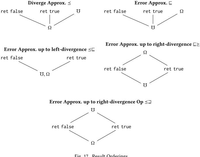Result Orderings <details> <summary>Image 8 Details</summary>  ### Visual Description ## Diagram: Result Orderings ### Overview The image presents a series of diagrams illustrating different result orderings related to divergence and error approximation. Each diagram depicts a directed graph with nodes labeled "ret false", "ret true", "Ω", and "υ", representing return values and approximation symbols. The diagrams show how these values and symbols are related under different approximation conditions. ### Components/Axes * **Nodes:** * "ret false": Represents the return value 'false'. * "ret true": Represents the return value 'true'. * "Ω": Represents a specific approximation symbol. * "υ": Represents a specific approximation symbol. * **Edges:** Directed lines connecting the nodes, indicating relationships or orderings. * **Titles:** Each diagram has a title indicating the type of approximation being represented: * "Diverge Approx. ≤" * "Error Approx. ⊆" * "Error Approx. up to left-divergence ⊆" * "Error Approx. up to right-divergence ⊇" * "Error Approx. up to right-divergence Op ⊆" * **Figure Caption:** "Fig. 17 Result Orderings" ### Detailed Analysis **1. Diverge Approx. ≤** * Nodes: "ret false" (top-left), "ret true" (top-right), "Ω" (bottom-center), "υ" (top-center). * Edges: "ret false" -> "Ω", "ret true" -> "Ω", "Ω" -> "υ". * Trend: Both "ret false" and "ret true" lead to "Ω", which then leads to "υ". **2. Error Approx. ⊆** * Nodes: "ret false" (top-left), "ret true" (top-right), "Ω" (top-center), "υ" (bottom-center). * Edges: "ret false" -> "υ", "ret true" -> "υ", "Ω" -> "υ". * Trend: Both "ret false" and "ret true" lead to "υ", and "Ω" also leads to "υ". **3. Error Approx. up to left-divergence ⊆** * Nodes: "ret false" (top-left), "ret true" (top-right), "υ, Ω" (bottom-center). * Edges: "ret false" -> "υ, Ω", "ret true" -> "υ, Ω". * Trend: Both "ret false" and "ret true" lead to the combined node "υ, Ω". **4. Error Approx. up to right-divergence ⊇** * Nodes: "ret false" (left), "ret true" (right), "Ω" (bottom-center), "υ" (top-center). * Edges: "υ" -> "ret false", "υ" -> "ret true", "ret false" -> "Ω", "ret true" -> "Ω". * Trend: "υ" leads to both "ret false" and "ret true", which both lead to "Ω". **5. Error Approx. up to right-divergence Op ⊆** * Nodes: "ret false" (left), "ret true" (right), "Ω" (bottom-center), "υ" (top-center). * Edges: "υ" -> "ret false", "υ" -> "ret true", "ret false" -> "Ω", "ret true" -> "Ω". * Trend: "υ" leads to both "ret false" and "ret true", which both lead to "Ω". ### Key Observations * The diagrams illustrate different relationships between return values ("ret false", "ret true") and approximation symbols ("Ω", "υ"). * The titles indicate the specific type of approximation being represented in each diagram. * The direction of the edges indicates the flow or ordering of the values and symbols. * The symbols "⊆" and "⊇" in the titles suggest subset and superset relationships, respectively. ### Interpretation The diagrams likely represent different strategies or methods for approximating results in a computational process. The "ret false" and "ret true" nodes probably represent the actual results of a computation, while "Ω" and "υ" represent approximations of those results. The diagrams show how these approximations relate to the actual results under different conditions, such as divergence or error. The "up to left/right-divergence" variations likely indicate different ways of handling divergence in the approximation process. The symbols "⊆" and "⊇" suggest that some approximations are subsets or supersets of the actual results, indicating the degree of accuracy or error in the approximation. The "Op" suffix may indicate an operation or operator applied during the approximation. </details> /precedesequal , which makes Ω a least element and every other element a maximal element. To distinguish these, we call /subsetsqequal error approximation and /precedesequal divergence approximation. We present these graphically (with two more) in Figure 17. The goal of this section is to prove that a symmetric equality E /supersetsqequal /subsetsqequal E ′ in CBPV (i.e. E /subsetsqequal E ′ and E ′ /subsetsqequal E ) implies contextual equivalence E = ctx E ′ and that inequality in CBPV E /subsetsqequal E ′ implies error approximation E /subsetsqequal ctx E ′ , proving graduality of the operational model: <!-- formula-not-decoded --> Because we have non-well-founded µ / ν types, we use a step-indexed logical relation to prove properties about the contextual lifting of certain preorders /triangleleftequal on results. In step-indexing, the infinitary relation given by /triangleleftequal ctx is related to the set of all of its finitary approximations /triangleleftequal i , which 'time out' after observing i steps of evaluation and declare that the terms are related. This means that the original relation is only recoverable from the finite approximations if Ω is always related to another element: if the relation is a preorder, we require that Ω is a least element. We call such a preorder a divergence preorder . Definition 6.8 (Divergence Preorder). A preorder on results /triangleleftequal is a divergence preorder if Ω /triangleleftequal R for all results R . But this presents a problem, because neither of our intended relations ( = and /subsetsqequal ) is a divergence preorder; rather both have Ω as a maximal element. However, there is a standard 'trick' for subverting this obstacle in the case of contextual equivalence [Ahmed 2006]: we notice that we can define equivalence as the symmetrization of divergence approximation, i.e., M = ctx N if and only if M /precedesequal ctx N and N /precedesequal ctx M , and since /precedesequal has Ω as a least element, we can use a step-indexed relation to prove it. As shown in New and Ahmed [2018], a similar trick works for error approximation, but since /subsetsqequal is not an equivalence relation, we decompose it rather into two different orderings: error approximation up to divergence on the left /precedesequal /subsetsqequal and error approximation up to divergence on the right /subsetsqequal /followsequal , also shown in figure 17. Note that /precedesequal /subsetsqequal is a preorder, but not a poset because /Omegainv , Ω are order-equivalent but not equal. Then clearly /precedesequal /subsetsqequal is a divergence preorder and the opposite of /subsetsqequal /followsequal , written /precedesequal /supersetsqequal is a divergence preorder. Then we can completely reduce the problem of proving = ctx and /subsetsqequal ctx results to proving results about divergence preorders by the following observations. Lemma 6.9 (Decomposing Result Preorders). Let R , S be results. - (1) R = S if and only if R /subsetsqequal S and S /subsetsqequal R . - (2) R = S if and only if R /precedesequal S and S /precedesequal R . - (3) R /precedesequal /subsetsqequal S iff R /subsetsqequal S or R /precedesequal S . - (4) R /subsetsqequal /followsequal S iff R /subsetsqequal S or R /followsequal S . In the following, we write ∼ ◦ for the opposite of a relation ( x ∼ ◦ y iff y ∼ x ), ⇒ for containment/implication ( ∼⇒∼ ′ iff x ∼ y implies x ∼ ′ y ), ⇔ for bicontainment/equality, ∨ for union ( x (∼ ∨ ∼ ′ ) y iff x ∼ y or x ∼ ′ y ), and ∧ for intersection ( x (∼ ∧ ∼ ′ ) y iff x ∼ y and x ∼ ′ y ). Lemma 6.10 (Contextual Lift commutes with Conjunction). <!-- formula-not-decoded --> Lemma 6.11 (Contextual Lift commutes with Dualization). <!-- formula-not-decoded --> Lemma 6.12 (Contextual Decomposition Lemma). Let ∼ be a reflexive relation ( = ⇒∼) , and /lessorequalslant be a reflexive, antisymmetric relation ( = ⇒ /lessorequalslant and ( /lessorequalslant ∧ /lessorequalslant ◦ ) ⇔ = ). Then <!-- formula-not-decoded --> Proof. Note that despite the notation, /lessorequalslant need not be assumed to be transitive. Reflexive relations form a lattice with ∧ and ∨ with = as ⊥ and the total relation as /latticetop (e.g. ( = ∨ ∼) ⇔∼ because ∼ is reflexive, and ( = ∧ ∼) ⇔ = ). So we have <!-- formula-not-decoded --> because FOILing the right-hand side gives <!-- formula-not-decoded --> By antisymmetry, ( /lessorequalslant ∧ /lessorequalslant ◦ ) is = , which is the unit of ∨ , so it cancels. By idempotence, (∼ ∧ ∼) is ∼ . Then by absorption, the whole thing is ∼ . Opposite is not de Morgan: ( P ∨ Q ) ◦ = P ◦ ∨ Q ◦ , and similarly for ∧ . But it is involutive: ( P ◦ ) ◦ ⇔ P . So using Lemmas 6.10, 6.11 we can calculate as follows: <!-- formula-not-decoded --> As a corollary, the decomposition of contextual equivalence into diverge approximation in Ahmed [2006] and the decomposition of dynamism in New and Ahmed [2018] are really the same trick: Corollary 6.13 (Contextual Decomposition). - (1) = ctx ⇔/precedesequal ctx ∧((/precedesequal) ctx ) ◦ - (2) = ctx ⇔/subsetsqequal ctx ∧((/subsetsqequal) ctx ) ◦ - (3) /subsetsqequal ctx ⇔/precedesequal/subsetsqequal ctx ∧((/precedesequal/supersetsqequal) ctx ) ◦ Proof. For part 1 (though we will not use this below), applying Lemma 6.12 with ∼ taken to be = (which is reflexive) and /lessorequalslant taken to be /precedesequal (which is reflexive and antisymmetric) gives that contextual equivalence is symmetric contextual divergence approximation: <!-- formula-not-decoded --> For part (2), the same argument with ∼ taken to be = and /lessorequalslant taken to be /subsetsqequal (which is also antisymmetric) gives that contextual equivalence is symmetric contextual dynamism: <!-- formula-not-decoded --> For part (3), applying Lemma 6.12 with ∼ taken to be /subsetsqequal and /lessorequalslant taken to be /precedesequal gives that dynamism decomposes as <!-- formula-not-decoded --> Since both /precedesequal /subsetsqequal and /precedesequal /supersetsqequal are of the form -∨ /precedesequal , both are divergence preorders. Thus, it suffices to develop logical relations for divergence preorders below. /square ## 6.3 CBPV Step Indexed Logical Relation Next, we turn to the problem of proving results about E /triangleleftequal ctx E ′ where /triangleleftequal is a divergence preorder. Dealing directly with a contextual preorder is practically impossible, so instead we develop an alternative formulation as a logical relation that is much easier to use. Fortunately, we can apply standard logical relations techniques to provide an alternate definition inductively on types. However, since we have non-well-founded type definitions using µ and ν , our logical relation will also be defined inductively on a step index that times out when we've exhausted our step budget. To bridge the gap between the indexed logical relation and the divergence preorder we care about, we define the 'finitization' of a divergence preorder to be a relation between programs and results : the idea is that a program approximates a result R at index i if it reduces to R in less than i steps or it reduces at least i times. Definition 6.14 (Finitized Preorder). Given a divergence preorder /triangleleftequal , we define the finitization of /triangleleftequal to be, for each natural number i , a relation between programs and results <!-- formula-not-decoded --> /Mapsto defined by <!-- formula-not-decoded --> /Mapsto Note that in this definition, unlike in the definition of divergence, we only count non-wellfounded steps. This makes it slightly harder to establish the intended equivalence M /triangleleftequal ω R if and only if result ( M ) /triangleleftequal R , but makes the logical relation theorem stronger: it proves that diverging terms must use recursive types of some sort and so any term that does not use them terminates. This issue would be alleviated if we had proved type safety by a logical relation rather than by progress and preservation. However, the following properties of the indexed relation can easily be established. First, a kind of 'transitivity' of the indexed relation with respect to the original preorder, which is key to proving transitivity of the logical relation. Lemma 6.15 (Indexed Relation is a Module of the Preorder). If M /triangleleftequal i R and R /triangleleftequal R ′ then M /triangleleftequal i R ′ /Mapsto Proof. If M ⇒ i M ′ then there's nothing to show, otherwise M ⇒ j < i result ( M ) so it follows by transitivity of the preorder: result ( M ) /triangleleftequal R /triangleleftequal R ′ . /square /Mapsto Then we establish a few basic properties of the finitized preorder. Lemma 6.16 (Downward Closure of Finitized Preorder). If M /triangleleftequal i R and j ≤ i then M /triangleleftequal j R . ## Proof. ``` ``` /Mapsto /Mapsto Next, we define the (closed) logical preorder (for closed values/stacks) by induction on types and the index i in figure 18. Specifically, for every i and value type A we define a relation /triangleleftequal log A , i between closed values of type A because these are the only ones that will be pattern-matched against at runtime. The relation is defined in a type-directed fashion, the intuition being that we relate two positive values when they are built up in the same way: i.e., they have the same introduction form and their subterms are related. For µ , this definition would not be well-founded, so we decrement the step index, giving up and relating the terms if i = 0. Finally U is the only negative value type, and so it is treated differently. A thunk V : UB cannot be inspected by pattern matching, rather the only way to interact with it is to force its evaluation. By the definition of the operational semantics, this only ever occurs in the step S [ force V ] , so (ignoring indices for a moment), we should define V 1 /triangleleftequal V 2 to hold in this case when, given S 1 /triangleleftequal S 2, the result of S 2 [ force V 2 ] is approximated by S 1 [ force V 1 ] . To incorporate the indices, we have to quantify over j ≤ i in this definition because we need to know that the values are related in all futures, including ones where some other part of the term has been reduced (consuming some steps). Technically, this is crucial for making sure the relation is downward-closed. This is known as the orthogonal of the relation, and one advantage of the CBPV language is that it makes the use of orthogonality explicit in the type structure, analogous to the benefits of using Nakano's later modality [Nakano [n. d.]] for step indexing (which we ironically do not do). /Mapsto Next, we define when two stacks are related. First, we define the relation only for two 'closed' stacks, which both have the same type of their hole B and both have 'output' the observation type F 2. The reason is that in evaluating a program M , steps always occur as S [ N ] ⇒ S [ N ′ ] where S is /Mapsto /Mapsto /Mapsto /Mapsto /Mapsto /Mapsto /Mapsto /Mapsto /Mapsto /Mapsto <!-- formula-not-decoded --> Fig. 18. Logical Relation from a Preorder /triangleleftequal a stack of this form. An intuition is that for negative types, two stacks are related when they start with the same elimination form and the remainder of the stacks are related. For ν , we handle the step indices in the same way as for µ . For FA , a stack S [· : FA ] is strict in its input and waits for its input to evaluate down to a value ret V , so two stacks with FA holes are related when in any future world, they produce related behavior when given related values. We note that in the CBV restriction of CBPV, the function type is given by U ( A → FA ′ ) and the logical relation we have presented reconstructs the usual definition that involves a double orthogonal. Note that the definition is well-founded using the lexicographic ordering on ( i , A ) and ( i , B ) : either the type reduces and the index stays the same or the index reduces. We extend the definition to contexts to closing substitutions pointwise: two closing substitutions for Γ are related at i if they are related at i for each x : A ∈ Γ . The logical preorder for open terms is defined as usual by quantifying over all related closing substitutions, but also over all stacks to the observation type F ( 1 + 1 ) : Definition 6.20 (Logical Preorder). For a divergence preorder /triangleleftequal , its step-indexed logical preorder is - (1) Γ /satisfies M 1 /triangleleftequal M 2 ∈ B iff for every γ 1 /triangleleftequal Γ γ 2 and S 1 /triangleleftequal S 2 , S 1 [ M 1 [ γ 1 ]] /triangleleftequal i result ( S 2 [ M 2 [ γ 2 ]]) . - (2) Γ /satisfies V 1 /triangleleftequal log V 2 ∈ A iff for every γ 1 /triangleleftequal log Γ , γ 2 , V 1 [ γ 1 ] /triangleleftequal log , V 2 [ γ 2 ] - (3) Γ | B /satisfies S 1 /triangleleftequal log i S 2 ∈ B ′ iff for every γ 1 /triangleleftequal log Γ , i γ 2 and S ′ 1 /triangleleftequal log B ′ , i S ′ 2 , S ′ 1 [ S 1 [ γ 1 ]] /triangleleftequal log B , i S ′ 2 [ S 2 [ γ 2 ]]) . ``` ``` We next want to prove that the logical preorder is a congruence relation, i.e., the fundamental lemma of the logical relation. This requires the easy lemma, that the relation on closed terms and stacks is downward closed. Lemma 6.21 (Logical Relation Downward Closure). For any type T , if j ≤ i then /triangleleftequal log , ⊆ /triangleleftequal log , T i T j Next, we show the fundamental theorem: Theorem 6.22 (Logical Preorder is a Congruence). For any divergence preorder, the logical preorder E /triangleleftequal log i E ′ is a congruence relation, i.e., it is closed under applying any value/term/stack constructors to both sides. Proof. For each congruence rule <!-- formula-not-decoded --> we prove for every i ∈ N the validity of the rule <!-- formula-not-decoded --> - (1) Γ , x : A , Γ ′ /satisfies x /triangleleftequal log i x ∈ A . Given γ 1 /triangleleftequal log Γ , x : A , Γ ′ , i γ 2, then by definition γ 1 ( x ) /triangleleftequal log A , i γ 2 ( x ) . - (2) Γ /satisfies /Omegainv /triangleleftequal log ∈ , /Omegainv B We need to show S 1 [ /Omegainv ] /triangleleftequal i result ( S 2 [ /Omegainv ]) . By anti-reduction and strictness of stacks, it is sufficient to show /Omegainv /triangleleftequal log i /Omegainv . If i = 0 there is nothing to show, otherwise, it follows by reflexivity of /triangleleftequal . log (3) Γ /satisfies V /triangleleftequal i V ′ ∈ A Γ , x : A /satisfies M /triangleleftequal i M ∈ B Γ /satisfies let x = V ; M /triangleleftequal log i let x = V ′ ; M ′ ∈ B Each side takes a 0-cost step, so by anti-reduction, this reduces to S 1 [ M [ γ 1 , V / x ]] /triangleleftequal i result ( S 2 [ M ′ [ γ 2 , V ′ / x ]]) log ′ which follows by the assumption Γ , x : A /satisfies M /triangleleftequal log i M ′ ∈ B - (5) Γ /satisfies V /triangleleftequal log i V ′ ∈ A 1 Γ /satisfies inl V /triangleleftequal log i inl V ′ ∈ A 1 + A 2 . Direct from assumption, rule for sums. log ′ ∈ - (4) Γ /satisfies V /triangleleftequal log i V ′ ∈ 0 Γ /satisfies abort V /triangleleftequal log i abort V ′ ∈ B . By assumption, we get V [ γ 1 ] /lessorsimilar i 0 , /Perpendicular V ′ [ γ 2 ] , but this is a contradiction. - (6) Γ /satisfies V /triangleleftequal i V A 2 Γ /satisfies inr V /triangleleftequal log i inr V ′ ∈ A 1 + A 2 Direct from assumption, rule for sums. By case analysis of V [ γ ] /triangleleftequal V ′ [ γ ] . - (7) Γ /satisfies V /triangleleftequal log i V ′ ∈ A 1 + A 2 Γ , x 1 : A 1 /satisfies M 1 /triangleleftequal log i M ′ 1 ∈ B Γ , x 2 : A 2 /satisfies M 2 /triangleleftequal log i M ′ 2 ∈ B Γ /satisfies case V { x 1 . M 1 | x 2 . M 2 } /triangleleftequal log i case V ′ { x 1 . M ′ 1 | x 2 . M ′ 2 } ∈ B log 2. (a) If V [ γ 1 ] = inl V 1 , V ′ [ γ 2 ] = inl V ′ 1 with V 1 /triangleleftequal log A 1 , i V ′ 1 , then taking 0 steps, by anti-reduction the problem reduces to 3. 1 i 2 <!-- formula-not-decoded --> which follows by assumption. - (b) For inr , the same argument. - (9) Γ /satisfies V 1 /triangleleftequal log i V ′ 1 ∈ A 1 Γ /satisfies V 2 /triangleleftequal log i V ′ 2 ∈ A 2 Γ /satisfies ( V , V ) /triangleleftequal log ( V ′ , V ′ ) ∈ A × A Immediate by pair rule. - (8) Γ /satisfies () /triangleleftequal log i () ∈ 1 Immediate by unit rule. - 1 2 i 1 2 1 2 - (10) Γ /satisfies V /triangleleftequal log i V ′ ∈ A 1 × A 2 Γ , x : A 1 , y : A 2 /satisfies M /triangleleftequal log i M ′ ∈ B Γ /satisfies split V to ( x , y ) . M /triangleleftequal log i split V ′ to ( x , y ) . M ′ ∈ B By V /triangleleftequal log A 1 × A 2 , i V ′ , we know V [ γ 1 ] = ( V 1 , V 2 ) and V ′ [ γ 2 ] = ( V ′ 1 , V ′ 2 ) with V 1 /triangleleftequal log A 1 , i V ′ 1 and V 2 /triangleleftequal log A 2 , i V ′ 2 . Then by antireduction, the problem reduces to <!-- formula-not-decoded --> which follows by assumption. - (11) Γ /satisfies V /triangleleftequal log i V ′ ∈ A [ µX . A / X ] Γ /satisfies roll µX . A V /triangleleftequal log i roll µX . A V ′ ∈ µX . A If i = 0, we're done. Otherwise i = j + 1, and our assumption is that V [ γ 1 ] /triangleleftequal log A [ µX . A / X ] , j + 1 V ′ [ γ 2 ] and we need to show that roll V [ γ 1 ] /triangleleftequal log µX . A , j + 1 roll V ′ [ γ 2 ] . By definition, we need to show V [ γ 1 ] /triangleleftequal log A [ µX . A / X ] , j V ′ [ γ 2 ] , which follows by downward-closure. - (12) Γ /satisfies V /triangleleftequal log i V ′ ∈ µX . A Γ , x : A [ µX . A / X ] /satisfies M /triangleleftequal log i M ′ ∈ B Γ /satisfies unroll V to roll x . M /triangleleftequal log i unroll V ′ to roll x . M ′ ∈ B If i = 0, then by triviality at 0, we're done. Otherwise, V [ γ 1 ] /triangleleftequal log µX . A , j + 1 V ′ [ γ 2 ] so V [ γ 1 ] = roll V µ , V ′ [ γ 2 ] = roll V ′ µ with V µ /triangleleftequal log A [ µX . A / X ] , j V ′ µ . Then each side takes 1 step, so by anti-reduction it is sufficient to show S 1 [ M [ γ 1 , V µ / x ]] /triangleleftequal j result ( S 2 [ M ′ [ γ 2 , V ′ µ / x ]]) which follows by assumption and downward closure of the stack, value relations. - (13) Γ /satisfies M /triangleleftequal log i M ′ ∈ B Γ /satisfies thunk M /triangleleftequal log i thunk M ′ ∈ UB . We need to show thunk M [ γ 1 ] /triangleleftequal log UB , i thunk M ′ [ γ 2 ] , so let S 1 /triangleleftequal log B , j S 2 for some j ≤ i , and we need to show <!-- formula-not-decoded --> Then each side reduces in a 0-cost step and it is sufficient to show <!-- formula-not-decoded --> Which follows by downward-closure for terms and substitutions. - (14) Γ /satisfies V /triangleleftequal log i V ′ ∈ UB Γ /satisfies force V /triangleleftequal log i force V ′ ∈ B . We need to show S 1 [ force V [ γ 1 ]] /triangleleftequal i result ( S 2 [ force V ′ [ γ 2 ]]) , which follows by the definition of V [ γ 1 ] /triangleleftequal log UB , i V ′ [ γ 2 ] . - (15) Γ /satisfies V /triangleleftequal log i V ′ ∈ A Γ /satisfies ret V /triangleleftequal log i ret V ′ ∈ FA We need to show S 1 [ ret V [ γ 1 ]] /triangleleftequal i result ( S 2 [ ret V ′ [ γ 2 ]]) , which follows by the orthogonality definition of S 1 /triangleleftequal log FA , i S 2 . <!-- formula-not-decoded --> We need to show bind x ← M [ γ 1 ] ; N [ γ 2 ] /triangleleftequal i result ( bind x ← M ′ [ γ 2 ] ; N ′ [ γ 2 ]) . By M /triangleleftequal log i M ′ ∈ FA , it is sufficient to show that <!-- formula-not-decoded --> So let j ≤ i and V /triangleleftequal log A , j V ′ , then we need to show <!-- formula-not-decoded --> By anti-reduction, it is sufficient to show <!-- formula-not-decoded --> which follows by anti-reduction for γ 1 /triangleleftequal log Γ , i γ 2 and N /triangleleftequal log i N ′ . <!-- formula-not-decoded --> <!-- formula-not-decoded --> By S 1 /triangleleftequal log A → B , i S 2, we know S 1 = S ′ 1 [· V 1 ] , S 2 = S ′ 2 [· V 2 ] with S ′ 1 /triangleleftequal log B , i S ′ 2 and V 1 /triangleleftequal log A , i V 2. Then by anti-reduction it is sufficient to show <!-- formula-not-decoded --> which follows by M /triangleleftequal log i M ′ . <!-- formula-not-decoded --> <!-- formula-not-decoded --> so by M /triangleleftequal log i M ′ it is sufficient to show S 1 [· V [ γ 1 ]] /triangleleftequal log A → B , i S 2 [· V ′ [ γ 2 ]] which follows by definition and assumption that V /triangleleftequal log i V ′ . <!-- formula-not-decoded --> - (19) Γ /turnstileleft {} : /latticetop We assume we are given S 1 /triangleleftequal log /latticetop , i S 2, but this is a contradiction. <!-- formula-not-decoded --> We proceed by case analysis of S 1 /triangleleftequal log B 1 & B 2 , i S 2 - (a) In the first possibility S 1 = S ′ 1 [ π ·] , S 2 = S ′ 2 [ π ·] and S ′ 1 /triangleleftequal log B 1 , i S ′ 2 . Then by anti-reduction, it is sufficient to show <!-- formula-not-decoded --> which follows by M 1 /triangleleftequal log i M ′ 1 . - (b) Same as previous case. - (21) Γ /satisfies M /triangleleftequal log i M ′ ∈ B 1 & B 2 Γ /satisfies πM /triangleleftequal log i πM ′ ∈ B 1 We need to show S 1 [ πM [ γ 1 ]] /triangleleftequal i result ( S 2 [ πM ′ [ γ 2 ]]) , which follows by S 1 [ π ·] /triangleleftequal log B 1 & B 2 , i S 2 [ π ·] and M /triangleleftequal log i M ′ . <!-- formula-not-decoded --> <!-- formula-not-decoded --> <!-- formula-not-decoded --> <!-- formula-not-decoded --> If i = 0, we invoke triviality at 0. Otherwise, i = j + 1 and we know by S 1 /triangleleftequal log νY . B , j + 1 S 2 that S 1 = S ′ 1 [ unroll ·] and S 2 = S ′ 2 [ unroll ·] with S ′ 1 /triangleleftequal log B [ νY . B / Y ] , j S ′ 2 , so by anti-reduction it is sufficient to show <!-- formula-not-decoded --> which follows by M /triangleleftequal log i M ′ and downward-closure. <!-- formula-not-decoded --> <!-- formula-not-decoded --> As a direct consequence we get the reflexivity of the relation <!-- formula-not-decoded --> so we have the following strengthening of the progress-and-preservation type soundness theorem: because /triangleleftequal i only counts unrolling steps, terms that never use µ or ν types (for example) are guaranteed to terminate. Corollary 6.24 (Unary LR). For every program · /turnstileleft M : F 2 and i ∈ N , M /triangleleftequal i result ( M ) Proof. By reflexivity, · /satisfies M /triangleleftequal i M ∈ F 2 and by definition · /triangleleftequal log F 2 , i · , so unrolling definitions we get M /triangleleftequal i result ( M ) . /square Using reflexivity, we prove that the indexed relation between terms and results recovers the original preorder in the limit as i → ω . We write /triangleleftequal ω to mean the relation holds for every i , i.e., /triangleleftequal ω = ⋂ i ∈ N /triangleleftequal i . Corollary 6.25 (Limit Lemma). For any divergence preorder /triangleleftequal , result ( M ) /triangleleftequal R iff M /triangleleftequal ω R . Proof. Two cases - (1) If result ( M ) /triangleleftequal R then we need to show for every i ∈ N , M /triangleleftequal i R . By the unary model lemma, M /triangleleftequal i result ( M ) , so the result follows by the module lemma 6.15. - (2) If M /triangleleftequal i R for every i , then there are two possibilities: M is always related to R because it takes i steps, or at some point M terminates. /Mapsto - (a) If M ⇒ i M i for every i ∈ N , then result ( M ) = Ω , so result ( M ) /triangleleftequal R because /triangleleftequal is a divergence preorder. so in particular /Mapsto - (b) Otherwise there exists some i ∈ M such that M ⇒ i result ( M ) , so it follows by the module lemma 6.15. /square Corollary 6.26 (Logical implies Contextual). If Γ /satisfies E /triangleleftequal log ω E ′ ∈ B then Γ /satisfies E /triangleleftequal ctx E ′ ∈ B . Proof. Let C be a closing context. By congruence, C [ M ] /triangleleftequal log ω C [ N ] , so using empty environment and stack, C [ M ] /triangleleftequal ω result ( C [ N ]) and by the limit lemma, we have result ( C [ M ]) /triangleleftequal result ( C [ N ]) . /square In fact, we can prove the converse, that at least for the term case, the logical preorder is complete with respect to the contextual preorder, though we don't use it. Lemma 6.27 (Contextual implies Logical). For any /triangleleftequal , if Γ /satisfies M /triangleleftequal ctx N ∈ B , then Γ /satisfies M /triangleleftequal log ω N ∈ B . Proof. Let S 1 /triangleleftequal log B , i S 2 and γ 1 /triangleleftequal log Γ , i γ 2. We need to show that <!-- formula-not-decoded --> So we need to construct a context that when M or N is plugged into the hole will reduce to the above. To do this, first, we deconstruct the context x 1 : A 1 , . . . , x n : A n = Γ . Then we define · /turnstileleft M ′ : A 1 →··· → A n → B as <!-- formula-not-decoded --> And similarly define N ′ . Then clearly <!-- formula-not-decoded --> /Mapsto <!-- formula-not-decoded --> and similarly for N ′ if x 1 , . . . , x n are all of the variables in γ . Then the proof proceeds by the following transitivity chain: S [ M [ γ ]] /triangleleftequal = /triangleleftequal = S ( result result S ( result result ( [ S ( M [ M S ′ [ N [ N γ [ γ γ ′ [ γ ]]) ( x ) ( x ]]) So S 1 [ M [ γ 1 ]] /triangleleftequal i result ( S 2 [ N [ γ 2 ]]) by the module lemma 6.15. log i /triangleleftequal M M ( ) (reduction) ( /triangleleftequal M N ) ctx (reduction) /square This establishes that our logical relation can prove graduality, so it only remains to show that our inequational theory implies our logical relation. Having already validated the congruence rules and reflexivity, we validate the remaining rules of transitivity, error, substitution, and βη for each type constructor. Other than the /Omegainv /subsetsqequal M rule, all of these hold for any divergence preorder. For transitivity, with the unary model and limiting lemmas in hand, we can prove that all of our logical relations (open and closed) are transitive in the limit. To do this, we first prove the following kind of 'quantitative' transitivity lemma, and then transitivity in the limit is a consequence. Lemma 6.28 (Logical Relation is /Q\_u.scantitatively Transitive). - (1) If V 1 /triangleleftequal log A , i V 2 and V 2 /triangleleftequal log A , ω V 3 , then V 1 /triangleleftequal log A , i V 3 - (2) If S 1 /triangleleftequal log B , i S 2 and S 2 /triangleleftequal log B , ω S 3 , then S 1 /triangleleftequal log B , i S 3 ) i /Mapsto · · · · · · γ γ ( x ( x n n )]) )]) Proof. Proof is by mutual lexicographic induction on the pair ( i , A ) or ( i , B ) . All cases are straightforward uses of the inductive hypotheses except the shifts U , F . - (1) If V 1 /triangleleftequal log UB , i V 2 and V 2 /triangleleftequal log UB , ω V 3, then we need to show that for any S 1 /triangleleftequal log B , j S 2 with j ≤ i , <!-- formula-not-decoded --> By reflexivity, we know S 2 /triangleleftequal log B , ω S 2, so by assumption <!-- formula-not-decoded --> which by the limiting lemma 6.25 is equivalent to <!-- formula-not-decoded --> so then by the module lemma 6.15, it is sufficient to show <!-- formula-not-decoded --> which holds by assumption. - (2) If S 1 /triangleleftequal log FA , i S 2 and S 2 /triangleleftequal log FA , ω S 3, then we need to show that for any V 1 /triangleleftequal log j , A V 2 with j ≤ i that <!-- formula-not-decoded --> First by reflexivity, we know V 2 /triangleleftequal log A , ω V 2, so by assumption, <!-- formula-not-decoded --> Which by the limit lemma 6.25 is equivalent to <!-- formula-not-decoded --> So by the module lemma 6.15, it is sufficient to show <!-- formula-not-decoded --> which holds by assumption. Lemma 6.29 (Logical Relation is /Q\_u.scantitatively Transitive (Open Terms)). - (1) If γ 1 /triangleleftequal log Γ , i γ 2 and γ 2 /triangleleftequal log Γ , ω γ 3 , then γ 1 /triangleleftequal log Γ , i γ 3 - (2) If Γ /satisfies M 1 /triangleleftequal log i M 2 ∈ B and Γ /satisfies M 2 /triangleleftequal log ω M 3 ∈ B , then Γ /satisfies M 1 /triangleleftequal log i M 3 ∈ B . - (4) If Γ | · : B /satisfies S 1 /triangleleftequal log i S 2 ∈ B ′ and Γ | · : B /satisfies S 2 /triangleleftequal log ω S 3 ∈ B ′ , then Γ | · : B /satisfies S 1 /triangleleftequal log i S 3 ∈ B ′ . - (3) If Γ /satisfies V 1 /triangleleftequal log i V 2 ∈ A and Γ /satisfies V 2 /triangleleftequal log ω V 3 ∈ A , then Γ /satisfies V 1 /triangleleftequal log i V 3 ∈ A . Proof. (1) By induction on the length of the context, follows from closed value case. - (2) Assume γ 1 /triangleleftequal log Γ , i γ 2 and S 1 /triangleleftequal log B , i S 2. We need to show <!-- formula-not-decoded --> by reflexivity and assumption, we know <!-- formula-not-decoded --> and by limit lemma 6.25, this is equivalent to <!-- formula-not-decoded --> so by the module lemma 6.15 it is sufficient to show <!-- formula-not-decoded --> /square which follows by assumption. - (3) Assume γ 1 /triangleleftequal log Γ , i γ 2. Then V 1 [ γ 1 ] /triangleleftequal log A , i V 2 [ γ 2 ] and by reflexivity γ 2 /triangleleftequal log Γ , ω γ 2 so V 2 [ γ 2 ] /triangleleftequal log A , ω V 3 [ γ 2 ] so the result holds by the closed case. - (4) Stack case is essentially the same as the value case. Corollary 6.30 (Logical Relation is Transitive in the Limit). - (1) If Γ /satisfies M 1 /triangleleftequal log ω M 2 ∈ B and Γ /satisfies M 2 /triangleleftequal log ω M 3 ∈ B , then Γ /satisfies M 1 /triangleleftequal log ω M 3 ∈ B . <!-- formula-not-decoded --> <!-- formula-not-decoded --> Next, we verify the β , η equivalences hold as orderings each way. Lemma 6.31 ( β , η ). For any divergence preorder, the β , η laws are valid for /triangleleftequal log ω Proof. The β rules for all cases except recursive types are direct from anti-reduction. - (1) µX . A -β : 2. (a) We need to show <!-- formula-not-decoded --> The left side takes 1 step to S 1 [ M [ γ 1 , V [ γ 1 ]/ x ]] and we know <!-- formula-not-decoded --> by assumption and reflexivity, so by anti-reduction we have <!-- formula-not-decoded --> so the result follows by downward-closure. - (b) For the other direction we need to show <!-- formula-not-decoded --> Since results are invariant under steps, this is the same as <!-- formula-not-decoded --> which follows by reflexivity and assumptions about the stacks and substitutions. - (2) µX . A -η : 2. (a) We need to show for any Γ , x : µX . A /turnstileleft M : B , and appropriate substitutions and stacks, S 1 [ unroll roll µX . A γ 1 ( x ) to roll y . M [ roll µX . A y / x ][ γ 1 ]] /triangleleftequal log i result ( S 2 [ M [ γ 2 ]]) By assumption, γ 1 ( x ) /triangleleftequal log µX . A , i γ 2 ( x ) , so we know <!-- formula-not-decoded --> <!-- formula-not-decoded --> and so the left side takes a step: S 1 [ unroll roll γ 1 ( x ) to roll y . M [ roll y / x ][ γ 1 ]] ⇒ 1 S 1 [ M [ roll y / x ][ γ 1 ][ V 1 / y ]] /Mapsto = S [ M [ roll = S 1 [ M [ γ 1 ]] V / x ][ γ ]] /square and by reflexivity and assumptions we know <!-- formula-not-decoded --> so by anti-reduction we know <!-- formula-not-decoded --> so the result follows by downward closure. - (b) Similarly, to show <!-- formula-not-decoded --> by the same reasoning as above, γ 2 ( x ) = roll µX . A V 2, so because result is invariant under reduction we need to show <!-- formula-not-decoded --> which follows by assumption and reflexivity. - (3) νY . B -β 2. (a) We need to show <!-- formula-not-decoded --> By the operational semantics, <!-- formula-not-decoded --> and by reflexivity and assumptions <!-- formula-not-decoded --> so the result follows by anti-reduction and downward closure. - (b) We need to show <!-- formula-not-decoded --> By the operational semantics and invariance of result under reduction this is equivalent to <!-- formula-not-decoded --> which follows by assumption. - (4) νY . B -η 2. (a) We need to show /Mapsto <!-- formula-not-decoded --> by assumption, S 1 /triangleleftequal log νY . B , i S 2 , so <!-- formula-not-decoded --> and therefore the left side reduces: <!-- formula-not-decoded --> and by assumption and reflexivity, <!-- formula-not-decoded --> so the result holds by anti-reduction and downward-closure. /Mapsto - (b) Similarly, we need to show <!-- formula-not-decoded --> as above, S 1 /triangleleftequal log νY . B , i S 2, so we know <!-- formula-not-decoded --> so <!-- formula-not-decoded --> and the result follows by reflexivity, anti-reduction and downward closure. - (5) 0 η Let Γ , x : 0 /turnstileleft M : B . 2. (a) We need to show <!-- formula-not-decoded --> By assumption γ 1 ( x ) /triangleleftequal log 0 , i γ 2 ( x ) but this is a contradiction - (b) Other direction is the same contradiction. - (6) + η . Let Γ , x : A 1 + A 2 /turnstileleft M : B - (a) We need to show S 1 [ case γ 1 ( x ){ x 1 . M [ inl x 1 / x ][ γ 1 ] | x 2 . M [ inr x 2 / x ][ γ 1 ]}] /triangleleftequal i result ( S 2 [ M [ γ 2 ]]) by assumption γ 1 ( x ) /triangleleftequal log A 1 + A 2 , i γ 2 ( x ) , so either it's an inl or inr . The cases are symmetric so assume γ 1 ( x ) = inl V 1. Then /Mapsto <!-- formula-not-decoded --> and so by anti-reduction it is sufficient to show <!-- formula-not-decoded --> which follows by reflexivity and assumptions. - (b) Similarly, We need to show result ( S 1 [ M [ γ 1 ]]) /triangleleftequal i result ( S 2 [ case γ 2 ( x ){ x 1 . M [ inl x 1 / x ][ γ 2 ] | x 2 . M [ inr x 2 / x ][ γ 2 ]}]) and by assumption γ 1 ( x ) /triangleleftequal log A 1 + A 2 , i γ 2 ( x ) , so either it's an inl or inr . The cases are symmetric so assume γ 2 ( x ) = inl V 2. Then /Mapsto <!-- formula-not-decoded --> So the result holds by invariance of result under reduction, reflexivity and assumptions. - (7) 1 η Let Γ , x : 1 /turnstileleft M : B 2. (a) We need to show <!-- formula-not-decoded --> By assumption γ 1 ( x ) /triangleleftequal log 1 , i γ 2 ( x ) so γ 1 ( x ) = () , so this is equivalent to <!-- formula-not-decoded --> which follows by reflexivity, assumption. - (b) Opposite case is similar. - (8) × η Let Γ , x : A 1 × A 2 /turnstileleft M : B - (a) We need to show <!-- formula-not-decoded --> <!-- formula-not-decoded --> <!-- formula-not-decoded --> <!-- formula-not-decoded --> /Mapsto <!-- formula-not-decoded --> So by anti-reduction it is sufficient to show <!-- formula-not-decoded --> which follows by reflexivity, assumption. - (b) Opposite case is similar. - (9) Uη Let Γ /turnstileleft V : UB - (a) We need to show that <!-- formula-not-decoded --> So assume S 1 /triangleleftequal log B , j S 2 for some j ≤ i , then we need to show <!-- formula-not-decoded --> The left side takes a step: <!-- formula-not-decoded --> so by anti-reduction it is sufficient to show <!-- formula-not-decoded --> which follows by assumption. - (b) Opposite case is similar. (10) Fη - (a) We need to show that given S 1 /triangleleftequal log FA , i S 2 , <!-- formula-not-decoded --> So assume V 1 /triangleleftequal log A , j V 2 for some j ≤ i , then we need to show <!-- formula-not-decoded --> The left side takes a step: <!-- formula-not-decoded --> so by anti-reduction it is sufficient to show <!-- formula-not-decoded --> which follows by assumption - (b) Opposite case is similar. <!-- formula-not-decoded --> /Mapsto /Mapsto - (a) We need to show <!-- formula-not-decoded --> by assumption that S 1 /triangleleftequal log A → B , i S 2, we know <!-- formula-not-decoded --> /Mapsto so the left side takes a step: <!-- formula-not-decoded --> So by anti-reduction it is sufficient to show <!-- formula-not-decoded --> which follows by reflexivity, assumption. - (b) Opposite case is similar. - (12) & η Let Γ /turnstileleft M : B 1 & B 2 - (a) We need to show <!-- formula-not-decoded --> by assumption, S 1 /triangleleftequal log B 1 & B 2 , i S 2 so either it starts with a π or π ′ so assume that S 1 = S ′ 1 [ π ·] ( π ′ case is similar). Then the left side reduces /Mapsto <!-- formula-not-decoded --> So by anti-reduction it is sufficient to show <!-- formula-not-decoded --> which follows by reflexivity, assumption. - (b) Opposite case is similar. - (13) /latticetop η Let Γ /turnstileleft M : /latticetop - (a) In either case, we assume we are given S 1 /triangleleftequal log /latticetop , i S 2, but this is a contradiction. <!-- formula-not-decoded --> /square Lemma 6.32 (Substitution Principles). For any diverge-bottom preorder /triangleleftequal , the following are valid Proof. We do the term case, the value case is similar. Given γ 1 /triangleleftequal log Γ , i γ 2, we have V 1 [ γ 1 ] /triangleleftequal log A , i V 2 [ γ 2 ] so <!-- formula-not-decoded --> and by associativity of substitution <!-- formula-not-decoded --> and similarly for M 2 , so if S 1 /triangleleftequal log B , i S 2 then <!-- formula-not-decoded --> For errors, the strictness axioms hold for any /triangleleftequal , but the axiom that /Omegainv is a least element is specific to the definitions of /precedesequal /subsetsqequal , /subsetsqequal /followsequal Lemma 6.33 (Error Rules). For any divergence preorder /triangleleftequal and appropriately typed S , M , <!-- formula-not-decoded --> /Mapsto Proof. (1) It is sufficient by the limit lemma to show result ( S [ /Omegainv ]) /triangleleftequal /Omegainv which holds by reflexivity because S [ /Omegainv ] ⇒ 0 /Omegainv . - (2) We need to show S [ /Omegainv ] /precedesequal /subsetsqequal i R for arbitrary R , so by the limit lemma it is sufficient to show /Omegainv /precedesequal /subsetsqequal R , which is true by definition. - (3) By the limit lemma it is sufficient to show R /precedesequal /supersetsqequal /Omegainv which is true by definition. /square The lemmas we have proved cover all of the inequality rules of CBPV, so applying them with /triangleleftequal chosen to be /precedesequal /subsetsqequal and /precedesequal /supersetsqequal gives Lemma 6.34 ( /precedesequal /subsetsqequal and /subsetsqequal /followsequal are Models of CBPV). If Γ | ∆ /turnstileleft E /subsetsqequal E ′ : B then Γ | ∆ /satisfies E /precedesequal /subsetsqequal ω E ′ ∈ B and Γ | ∆ /satisfies E ′ /precedesequal /supersetsqequal ω E ∈ B . Because logical implies contextual equivalence, we can conclude with the main theorem: Theorem 6.35 (Contextual Approximation/E/q.sc\_u.scivalence Model CBPV). <!-- formula-not-decoded --> Proof. For the first part, from Lemma 6.34, we have E /precedesequal /subsetsqequal ω E ′ and E ′ /precedesequal /supersetsqequal ω E . By Lemma 6.26, we then have E /precedesequal /subsetsqequal ctx E ′ and E ′ /precedesequal /supersetsqequal ctx E . Finally, by Corollary 6.13, E /subsetsqequal ctx E ′ iff E /precedesequal /subsetsqequal ctx E ′ and E ((/precedesequal /supersetsqequal) ctx ) ◦ E ′ , so we have the result. For the second part, applying the first part twice gives E /subsetsqequal ctx E ′ and E ′ /subsetsqequal ctx E , and we concluded in Corollary 6.13 that this coincides with contextual equivalence. /square ## 7 DISCUSSION AND RELATED WORK In this paper, we have given a logic for reasoning about gradual programs in a mixed call-byvalue/call-by-name language, shown that the axioms uniquely determine almost all of the contract translation implementing runtime casts, and shown that the axiomatics is sound for contextual equivalence/approximation in an operational model. In immediate future work, we believe it is straightforward to add inductive/coinductive types and obtain similar unique cast implementation theorems (e.g. 〈 list ( A ′ ) /arrowtailleft list ( A )〉 /supersetsqequal/subsetsqequal map 〈 A ′ /arrowtailleft A 〉 ). Additionally, since more efficient cast implementations such as optimized cast calculi (the lazy variant in Herman et al. [2010]) and threesome casts [Siek and Wadler 2010], are equivalent to the lazy contract semantics, they should also be models of GTT, and if so we could use GTT to reason about program transformations and optimizations in them. Applicability of Cast Uniqueness Principles. The cast uniqueness principles given in theorem 3.15 are theorems in the formal logic of Gradual Type Theory, and so there is a question of to what languages the theorem applies. The theorem applies to any model of gradual type theory, such as the models we have constructed using call-by-push-value given in Sections 4, 5, 6. We conjecture that simple call-by-value and call-by-name gradual languages are also models of GTT, by extending the translation of call-by-push-value into call-by-value and call-by-name in the appendix of Levy's monograph [Levy 2003]. In order for the theorem to apply, the language must validate an appropriate version of the η principles for the types. So for example, a call-by-value language that has reference equality of functions does not validate even the value-restricted η law for functions, and so the case for functions does not apply. It is a well-known issue that in the presence of pointer equality of functions, the lazy semantics of function casts is not compatible with the graduality property, and our uniqueness theorem provides a different perspective on this phenomenon [Findler et al. 2004; Strickland et al. 2012; Siek et al. 2015a]. However, we note that the cases of the uniqueness theorem for each type connective are completely modular : they rely only on the specification of casts and the β , η principles for the particular connective, and not on the presence of any other types, even the dynamic types. So even if a call-by-value language may have reference equality functions, if it has the η principle for strict pairs, then the pair cast must be that of Theorem 3.15. Next, we consider the applicability to non-eager languages. Analogous to call-by-value, our uniqueness principle should apply to simple call-by-name gradual languages, where full η equality for functions is satisfied, but η equality for booleans and strict pairs requires a 'stack restriction' dual to the value restriction for call-by-value function η . We are not aware of any call-by-name gradual languages, but there is considerable work on contracts for non-eager languages, especially Haskell [Hinze et al. 2006; Xu et al. 2009]. However, we note that Haskell is not a call-by-name language in our sense for two reasons. First, Haskell uses call-by-need evaluation where results of computations are memoized. However, when only considering Haskell's effects (error and divergence), this difference is not observable so this is not the main obstacle. The bigger difference between Haskell and call-by-name is that Haskell supports a seq operation that enables the programmer to force evaluation of a term to a value. This means Haskell violates the function η principle because Ω will cause divergence under seq , whereas λx . Ω will not. This is a crucial feature of Haskell and is a major source of differences between implementations of lazy contracts, as noted in Degen et al. [2012]. We can understand this difference by using a different translation into call-by-push-value: what Levy calls the 'lazy paradigm', as opposed to call-by-name [Levy 2003]. Simply put, connectives are interpreted as in call-by-value, but with the addition of extra thunks UF , so for instance the lazy function type A → B is interpreted as UFU ( UFA → FB ) and the extra UFU here is what causes the failure of the call-by-name η principle. With this embedding and the uniqueness theorem, GTT produces a definition for lazy casts, and the definition matches the work of Xu et al. [2009] when restricting to non-dependent contracts. Comparing Soundness Principles for Cast Semantics. Greenman and Felleisen [2018] gives a spectrum of differing syntactic type soundness theorems for different semantics of gradual typing. Our work here is complementary, showing that certain program equivalences can only be achieved by certain cast semantics. Degen et al. [2012] give an analysis of different cast semantics for contracts in lazy languages, specifically based on Haskell, i.e., call-by-need with seq . They propose two properties 'meaning preservation' and 'completeness' that they show are incompatible and identify which contract semantics for a lazy language satisfy which of the properties. The meaning preservation property is closely related to graduality: it says that evaluating a term with a contract either produces blame or has the same observable effect as running the term without the contract. Meaning preservation rules out overly strict contract systems that force (possibly diverging) thunks that wouldn't be forced in a non-contracted term. Completeness, on the other hand, requires that when a contract is attached to a value that it is deeply checked. The two properties are incompatible because, for instance, a pair of a diverging term and a value can't be deeply checked without causing the entire program to diverge. Using Levy's embedding of the lazy paradigm into call-by-push-value their incompatibility theorem should be a consequence of our main theorem in the following sense. We showed that any contract semantics departing from the implementation in Theorem 3.15 must violate η or graduality. Their completeness property is inherently eager, and so must be different from the semantics GTT would provide, so either the restricted η or graduality fails. However, since they are defining contracts within the language, they satisfy the restricted η principle provided by the language, and so it must be graduality, and therefore meaning preservation that fails. Axiomatic Casts. Henglein's work on dynamic typing also uses an axiomatic semantics of casts, but axiomatizes behavior of casts at each type directly whereas we give a uniform definition of all casts and derive implementations for each type [Henglein 1994]. Because of this, the theorems proven in that paper are more closely related to our model construction in Section 4. More specifically, many of the properties of casts needed to prove Theorem 4.23 have direct analogues in Henglein's work, such as the coherence theorems. We have not included these lemmas in the paper because they are quite similar to lemmas proven in New and Ahmed [2018]; see there for a more detailed comparison, and the extended version of this paper for full proof details [New et al. 2018]. Finally, we note that our assumption of compositionality, i.e., that all casts can be decomposed into an upcast followed by a downcast, is based on Henglein's analysis, where it was proven to hold in his coercion calculus. Gradual Typing Frameworks. In this work we have applied a method of 'gradualizing' axiomatic type theories by adding in dynamism orderings and adding dynamic types, casts and errors by axioms related to the dynamism orderings. This is similar in spirit to two recent frameworks for designing gradual languages: Abstracting Gradual Typing (AGT) [Garcia et al. 2016] and the Gradualizer [Cimini and Siek 2016, 2017]. All of these approaches start with a typed language and construct a related gradual language. A major difference between our approach and those is that our work is based on axiomatic semantics and so we take into account the equality principles of the typed language, whereas Gradualizer is based on the typing and operational semantics and AGT is based on the type safety proof of the typed language. Furthermore, our approach produces not just a single language, but also an axiomatization of the structure of gradual typing and so we can prove results about many languages by proving theorems in GTT. The downside to this is that our approach doesn't directly provide an operational semantics for the gradual language, whereas for AGT this is a semi-mechanical process and for Gradualizer, completely automated. Finally, we note that AGT produces the 'eager' semantics for function types, and it is not clear how to modify the AGT methodology to reproduce the lazy semantics that GTT provides. More generally, both AGT and the Gradualizer are known to produce violations of parametricity when applied to polymorphic languages, with the explanation being that the parametricity property is in no way encoded in the input to the systems: the operational semantics and the type safety proof. In future work, we plan to apply our axiomatic approach to gradualizing polymorphism and state by starting with the rich relational logics and models of program equivalence for these features [Plotkin and Abadi 1993; Dunphy 2002; Matthews and Ahmed 2008; Neis et al. 2009; Ahmed et al. 2009], which may lend insight into existing proposals [Siek et al. 2015b; Ahmed et al. 2017; Igarashi et al. 2017a; Siek and Taha 2006]- for example, whether the 'monotonic' [Siek et al. 2015b] and 'proxied' [Siek and Taha 2006] semantics of references support relational reasoning principles of local state. Blame. We do not give a treatment of runtime blame reporting, but we argue that the observation that upcasts are thunkable and downcasts are linear is directly related to blame soundness [Tobin-Hochstadt and Felleisen 2006; Wadler and Findler 2009] in that if an upcast were not thunkable, it should raise positive blame and if a downcast were not linear, it should raise negative blame. First, consider a potentially effectful stack upcast of the form 〈 FA ′ /arrowtailleft FA 〉 . If it is not thunkable, then in our logical relation this would mean there is a value V : A such that 〈 FA ′ /arrowtailleft FA 〉( ret V ) performs some effect. Since the only observable effects for casts are dynamic type errors, 〈 FA ′ /arrowtailleft FA 〉( ret V ) ↦→ /Omegainv , and we must decide whether the positive party or negative party is at fault. However, since this is call-by-value evaluation, this error happens unconditionally on the continuation, so the continuation never had a chance to behave in such a way as to prevent blame, and so we must blame the positive party. Dually, consider a value downcast of the form 〈 UB /dblarrowheadleft UB ′ 〉 . If it is not linear, that would mean it forces its UB ′ input either never or more than once. Since downcasts should refine their inputs, it is not possible for the downcast to use the argument twice, since e.g. printing twice does not refine printing once. So if the cast is not linear, that means it fails without ever forcing its input, in which case it knows nothing about the positive party and so must blame the negative party. In future work, we plan to investigate extensions of GTT with more than one /Omegainv with different blame labels, and an axiomatic account of a blame-aware observational equivalence. Denotational and Category-theoretic Models. Wehave presented certain concrete models of GTT using ordered CBPV with errors, in order to efficiently arrive at a concrete operational interpretation. It may be of interest to develop a more general notion of model of GTT for which we can prove soundness and completeness theorems, as in New and Licata [2018]. A model would be a strong adjunction between double categories where one of the double categories has all 'companions' and the other has all 'conjoints', corresponding to our upcasts and downcasts. Then the contract translation should be a construction that takes a strong adjunction between 2-categories and makes a strong adjunction between double categories where the ep pairs are 'Kleisli' ep pairs: the upcast is has a right adjoint, but only in the Kleisli category and vice-versa the downcast has a left adjoint in the co-Kleisli category. Furthermore, the ordered CBPV with errors should also have a sound and complete notion of model, and so our contract translation should have a semantic analogue as well. Gradual Session Types. Gradual session types [Igarashi et al. 2017b] share some similarities to GTT, in that there are two sorts of types (values and sessions) with a dynamic value type and a dynamic session type. However, their language is not polarized in the same way as CBPV, so there is not likely an analogue between our upcasts always being between value types and downcasts always being between computation types. Instead, we might reconstruct this in a polarized session type language [Pfenning and Griffith 2015]. The two dynamic types would then be the 'universal sender' and 'universal receiver' session types. Dynamically Typed Call-by-push-value. Our interpretation of the dynamic types in CBPV suggests a design for a Scheme-like language with a value and computation distinction. This may be of interest for designing an extension of Typed Racket that efficiently supports CBN or a Schemelike language with codata types. While the definition of the dynamic computation type by a lazy product may look strange, we argue that it is no stranger than the use of its dual, the sum type, in the definition of the dynamic value type. That is, in a truly dynamically typed language, we would not think of the dynamic type as being built out of some sum type construction, but rather that it is the union of all of the ground value types, and the union happens to be a disjoint union and so we can model it as a sum type. In the dual, we don't think of the computation dynamic type as a product , but instead as the intersection of the ground computation types. Thinking of the type as unfolding: <!-- formula-not-decoded --> This says that a dynamically typed computation is one that can be invoked with any finite number of arguments on the stack, a fairly accurate model of implementations of Scheme that pass multiple arguments on the stack. Dependent Contract Checking. We also plan to explore using GTT's specification of casts in a dependently typed setting, building on work using Galois connections for casts between dependent types [Dagand et al. 2018], and work on effectful dependent types based a CBPV-like judgement structure [Ahman et al. 2016]. Acknowledgments. We thank Ron Garcia, Kenji Maillard and Gabriel Scherer for helpful discussions about this work. We thank the anonymous reviewers for helpful feedback on this article. This material is based on research sponsored by the National Science Foundation under grant CCF1453796 and the United States Air Force Research Laboratory under agreement number FA955015-1-0053 and FA9550-16-1-0292. The views and conclusions contained herein are those of the authors and should not be interpreted as necessarily representing the official policies or endorsements, either expressed or implied, of the United States Air Force Research Laboratory, the U.S. Government, or Carnegie Mellon University. ## REFERENCES - Danel Ahman, Neil Ghani, and Gordon D. Plotkin. 2016. Dependent Types and Fibred Computational Effects. In Foundations of Software Science and Computation Structures . 36-54. - Amal Ahmed. 2006. Step-Indexed Syntactic Logical Relations for Recursive and Quantified Types. In European Symposium on Programming (ESOP) . 69-83. - Amal Ahmed, Derek Dreyer, and Andreas Rossberg. 2009. State-Dependent Representation Independence. In ACMSymposium on Principles of Programming Languages (POPL), Savannah, Georgia . - Amal Ahmed, Dustin Jamner, Jeremy G. Siek, and Philip Wadler. 2017. Theorems for Free for Free: Parametricity, With and Without Types. In International Conference on Functional Programming (ICFP), Oxford, United Kingdom . - Jean-Marc Andreoli. 1992. Logic programming with focusing proofs in linear logic. Journal of Logic and Computation 2, 3 (1992), 297-347. - Andrej Bauer and Matija Pretnar. 2013. An Effect System for Algebraic Effects and Handlers. In Algebra and Coalgebra in Computer Science . Springer Berlin Heidelberg, Berlin, Heidelberg, 1-16. - Matteo Cimini and Jeremy G. Siek. 2016. The Gradualizer: A Methodology and Algorithm for Generating Gradual Type Systems. In Proceedings of the 43rd Annual ACM SIGPLAN-SIGACT Symposium on Principles of Programming Languages (POPL '16) . - Matteo Cimini and Jeremy G. Siek. 2017. Automatically Generating the Dynamic Semantics of Gradually Typed Languages. In Proceedings of the 44th ACM SIGPLAN Symposium on Principles of Programming Languages (POPL 2017) . 789-803. - Pierre-Èvariste Dagand, Nicolas Tabareau, and Èric Tanter. 2018. Foundations of dependent interoperability. Journal of Functional Programming 28 (2018), e9. https://doi.org/10.1017/S0956796818000011 - Markus Degen, Peter Thiemann, and Stefan Wehr. 2012. The interaction of contracts and laziness. Higher-Order and Symbolic Computation 25 (2012), 85-125. - Brian Patrick Dunphy. 2002. Parametricity As a Notion of Uniformity in Reflexive Graphs . Ph.D. Dissertation. Champaign, IL, USA. Advisor(s) Reddy, Uday. - Robert Bruce Findler and Matthias Felleisen. 2002. Contracts for higher-order functions. In International Conference on Functional Programming (ICFP) . 48-59. - Robert Bruce Findler, Matthew Flatt, and Matthias Felleisen. 2004. Semantic Casts: Contracts and Structural Subtyping in a Nominal World. In European Conference on Object-Oriented Programming (ECOOP) . - Carsten Führmann. 1999. Direct models of the computational lambda-calculus. Electronic Notes in Theoretical Computer Science 20 (1999), 245-292. Ronald Garcia, Alison M. Clark, and Éric Tanter. 2016. Abstracting Gradual Typing. In ACM Symposium on Principles of Programming Languages (POPL) . Jean-Yves Girard. 2001. Locus Solum: From the rules of logic to the logic of rules. Mathematical Structures in Computer Science 11, 3 (2001), 301âĂŞ506. Michael Greenberg. 2015. Space-Efficient Manifest Contracts. In ACM Symposium on Principles of Programming Languages (POPL) . 181-194. Michael Greenberg, Benjamin C. Pierce, and Stephanie Weirich. 2010. Contracts Made Manifest (POPL '10) . Ben Greenman and Matthias Felleisen. 2018. A Spectrum of Type Soundness and Performance. In International Conference on Functional Programming (ICFP), St. Louis, Missouri . Fritz Henglein. 1994. Dynamic Typing: Syntax and Proof Theory. 22, 3 (1994), 197-230. David Herman, Aaron Tomb, and Cormac Flanagan. 2010. Space-efficient gradual typing. Higher-Order and Symbolic Computation (2010). Ralf Hinze, Johan Jeuring, and Andres Löh. 2006. Typed Contracts for Functional Programming. In International Symposium on Functional and Logic Programming (FLOPS) . Atsushi Igarashi, Peter Thiemann, Vasco T. Vasconcelos, and Philip Wadler. 2017b. Gradual Session Types. Proceedings of ACM Programning Languages 1, ICFP, Article 38 (Aug. 2017), 28 pages. Yuu Igarashi, Taro Sekiyama, and Atsushi Igarashi. 2017a. On Polymorphic Gradual Typing. In International Conference on Functional Programming (ICFP), Oxford, United Kingdom . Paul Blain Levy. 2003. Call-By-Push-Value: A Functional/Imperative Synthesis . Springer. Paul Blain Levy. 2017. Contextual Isomorphisms. In ACM Symposium on Principles of Programming Languages (POPL) . Sam Lindley, Conor McBride, and Craig McLaughlin. 2017. Do Be Do Be Do. In Proceedings of the 44th ACM SIGPLAN Symposium on Principles of Programming Languages (POPL 2017) . ACM, 500-514. Jacob Matthews and Amal Ahmed. 2008. Parametric polymorphism through run-time sealing, or, Theorems for low, low prices!. In European Symposium on Programming (ESOP) . Eugenio Moggi. 1991. Notions of computation and monads. Inform. And Computation 93, 1 (1991). Guillaume Munch-Maccagnoni. 2014. Models of a Non-associative Composition. In Foundations of Software Science and Computation Structures . 396-410. Hiroshi Nakano. [n. d.]. A modality for recursion. In Logic in Computer Science, 2000. Proceedings. 15th Annual IEEE Symposium on . Georg Neis, Derek Dreyer, and Andreas Rossberg. 2009. Non-Parametric Parametricity. In International Conference on Functional Programming (ICFP) . 135-148. MaxS. New and Amal Ahmed. 2018. Graduality from Embedding-Projection Pairs. In International Conference on Functional Programming (ICFP), St. Louis, Missouri . Max S. New and Daniel R. Licata. 2018. Call-by-name Gradual Type Theory. FSCD (2018). Max S. New, Daniel R. Licata, and Amal Ahmed. 2018. Gradual Type Theory (Extend Version). (2018). arxiv:. Frank Pfenning and Dennis Griffith. 2015. Polarized Substructural Session Types (invited talk). In International Conference on Foundations of Software Science and Computation Structures (FoSSaCS) . Gordon D. Plotkin and Martín Abadi. 1993. A Logic for Parametric Polymorphism. In Typed Lambda Calculi and Applications, International Conference on Typed Lambda Calculi and Applications, TLCA '93, Utrecht, The Netherlands, March 16-18, 1993, Proceedings . 361-375. Jeremy Siek, Ronald Garcia, and Walid Taha. 2009. Exploring the Design Space of Higher-Order Casts. In European Symposium on Programming (ESOP) . Springer-Verlag, Berlin, Heidelberg, 17-31. Jeremy Siek and Sam Tobin-Hochstadt. 2016. The recursive union of some gradual types. A List of Successes That Can Change the World: Essays Dedicated to Philip Wadler on the Occasion of His 60th Birthday (Springer LNCS) volume 9600 (2016). Jeremy Siek, Micahel Vitousek, Matteo Cimini, and John Tang Boyland. 2015a. Refined Criteria for Gradual Typing. In 1st Summit on Advances in Programming Languages (SNAPL 2015) . Jeremy G. Siek and Walid Taha. 2006. Gradual Typing for Functional Languages. In Scheme and Functional Programming Workshop (Scheme) . 81-92. Jeremy G. Siek, Michael M. Vitousek, Matteo Cimini, Sam Tobin-Hochstadt, and Ronald Garcia. 2015b. Monotonic References for Efficient Gradual Typing. In Proceedings of the 24th European Symposium on Programming on Programming Languages and Systems - Volume 9032 . Jeremy G. Siek and Philip Wadler. 2010. Threesomes, with and Without Blame. In ACM Symposium on Principles of Programming Languages (POPL) . ACM, 365-376. T. Stephen Strickland, Sam Tobin-Hochstadt, Robert Bruce Findler, and Matthew Flatt. 2012. Chaperones and Impersonators: Run-time Support for Reasonable Interposition (ACM Symposium on Object Oriented Programming: Systems, Languages, - and Applications (OOPSLA)) . Sam Tobin-Hochstadt and Matthias Felleisen. 2006. Interlanguage Migration: From Scripts to Programs. In Dynamic Languages Symposium (DLS) . 964-974. Michael M. Vitousek, Cameron Swords, and Jeremy G. Siek. 2017. Big Types in Little Runtime: Open-world Soundness and Collaborative Blame for Gradual Type Systems (POPL 2017) . Philip Wadler and Robert Bruce Findler. 2009. Well-typed programs can't be blamed. In European Symposium on Programming (ESOP) . 1-16. Dana N. Xu, Simon Peyton Jones, and Koen Claessen. 2009. Static Contract Checking for Haskell (ACM Symposium on Principles of Programming Languages (POPL), Savannah, Georgia) . Noam Zeilberger. 2009. The Logical Basis of Evaluation Order and Pattern-Matching. Ph.D. Dissertation. Carnegie Mellon University.