1811.08210v1

# ArXiv Paper 1811.08210v1 ## Brain-Inspired Stigmergy Learning Xing Hsu, Zhifeng Zhao, Rongpeng Li, Honggang Zhang College of Information Science and Electronic Engineering Zhejiang University, Zheda Road 38, Hangzhou 310027, China Emails: { hsuxing, zhaozf, lirongpeng, honggangzhang } @zju.edu.cn Abstract -Stigmergy has proved its great superiority in terms of distributed control, robustness and adaptability, thus being regarded as an ideal solution for large-scale swarm control problems. Based on new discoveries on astrocytes in regulating synaptic transmission in the brain, this paper has mapped stigmergy mechanism into the interaction between synapses and investigated its characteristics and advantages. Particularly, we have divided the interaction between synapses which are not directly connected into three phases and proposed a stigmergic learning model. In this model, the state change of a stigmergy agent will expand its influence to affect the states of others. The strength of the interaction is determined by the level of neural activity as well as the distance between stigmergy agents. Inspired by the morphological and functional changes in astrocytes during environmental enrichment, it is likely that the regulation of distance between stigmergy agents plays a critical role in the stigmergy learning process. Simulation results have verified its importance and indicated that the well-regulated distance between stigmergy agents can help to obtain stigmergy learning gain. Index Terms -Stigmergy, Astrocytes, Synapses, Calcium Waves, Neural Networks, Artificial Intelligence, Machine Learning ## I. INTRODUCTION Stigmergy was first introduced by French entomologist Pierre-Paul Grass` e in 1950s [1] [2] when studying the behavior of social insects. The word stigmergy is a combination of the Greek words 'stigma' (outstanding sign) and 'ergon' (work), indicating that some activities of agents are triggered by external signs, which themselves may be generated by agent activities [3]. Stigmergy allowed Grass` e to explain why insects of very limited intelligence, without apparent communications, can collaboratively tackle complex tasks, such as building a nest. Another definition given by Heylighen is [4]: stigmergy is an indirect, mediated mechanism of coordination between actions in which a perceived effect of an action stimulates the performance of a subsequent action. Stigmergy has been widely studied in the behavior of social insects [5] [6]. But this concept is rarely mentioned in the brain, which has been regarded as the most complex system so far. As important glial cells in brain's Central Nervous System (CNS), astrocytes are traditionally placed in a subservient position, which supports the physiology of the associated neurons. However, recent experimental neuroscience evidences indicate that astrocytes also interact closely with neurons and participate in the regulation of synaptic neurotransmission [7]. These evidences have motivated new perspectives for the research of stigmergy in the brain. 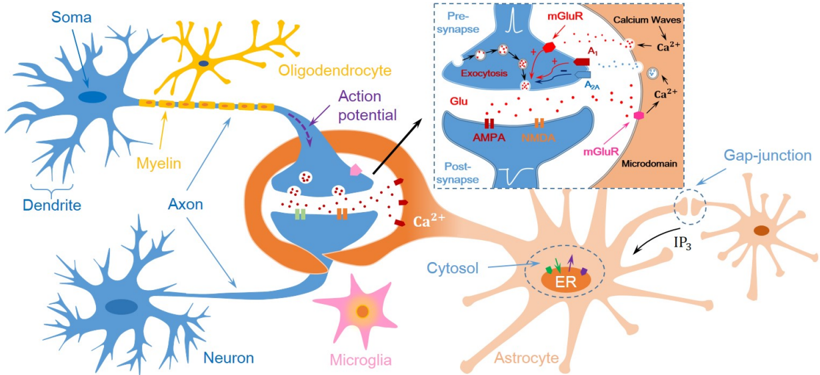There is a large number of complicated biochemical reactions between synapses and astrocytes to support the implementation of various brain functions. Basically, each astrocyte contains hundreds or thousands of branch microdomains, and each of them encloses a synapse [8], as illustrated in Fig. 1. The synaptic activity will elevate the concentration of Ca 2+ in the corresponding microdomain. Ca 2+ and inositol-1,4,5triphospate ( IP 3 ), as important messengers within astrocytes, are believed to expand the influence of synaptic activities [9]. The range of influence is determined by the level of synaptic activity as well as the distance between coupled branch microdomains. Besides, these branch microdomains with the elevated concentration of Ca 2+ will provide an adjustment for the wrapped synapses. Therefore, as explained in Section II, general stigmergy can be mapped into this neural process in which astrocytes play the role of medium carriers to provide adjustments for the involved synapses. The interaction between several synapses, which is mainly mediated by the propagation of Ca 2+ in cytosol within astrocytes, can be divided into three important phases. These phases will be concretely described in Section III so as to constitute the stigmergic system model. In this fundamental model, the strength of interaction between stigmergy agents is determined by the level of stimulations as well as the distance between them, which is consistent with the strength of interaction between synapses via astrocytes. Inspired by the morphological and functional changes in astrocytes during environmental enrichment, it is likely that the regulation of distance between stigmergy agents is critical to obtain stigmergy learning gain. Accordingly, the importance of the regulation is verified in two different stigmergic scenarios. The remainder of this paper is organized as follows. In Section II, new discoveries on astrocytes in regulating synaptic transmission will be introduced and the existence of general stigmergy in the brain will be explored. In Section III, three important phases within the interaction between synapses will be described. The interaction is referred to set up the stigmergic system model and learning algorithm. In Section IV, the simulations on the performance of the proposed stigmergy learning are carried out in two different stigmergic scenarios, in order to verify its effectiveness and advantages. Finally, we conclude this paper with a summary. ## II. STIGMERGY IN THE BRAIN In CNS, general stigmergy can be mapped into the interaction between synapses, which is mainly mediated by Ca 2+ within astrocytes. As important medium carriers, astrocytes are coupled together by the gap-junction to comprise a nervous regulation. ## A. Glial Cells in CNS In the process of nerve conduction, action potentials represented by the purple dotted arrow in Fig. 1 are conducted along the axon to the pre-synaptic terminal. Then a large quantity of neurotransmitters will be released into synaptic cleft through exocytosis. These molecules will diffuse and bind with various receptors on the surface of post-synaptic terminal. Besides, they can also diffuse and bind with receptors of surrounding glial cells, which will release neuromodulators in return [10]. In essential, there are three types of glial cells in CNS: microglia, oligodendrocytes, and astrocytes [11]. Microglia, as illustrated in Fig. 1, are macrophages in CNS. Their key roles are immune surveillance as well as responding to infections or other pathological states such as neurological diseases or injury [12] [13]. For the synaptic activity, microglia play the role of supervision and protection. Oligodendrocytes can contribute to the plasticity of nervous systems in the process of nerve conduction. An action potential needs to spend a certain amount of time reaching the presynaptic terminal. Many factors affect the conduction velocity, such as the thickness of myelin sheath, the axon diameter and the spacing and width of the Ranvier nodes [14]. Increasing the thickness of myelin sheath can significantly improve the velocity, which helps to form the saltatory conduction. In this way, high-speed nerve pulses jump along the axon towards the pre-synaptic terminal, leading to a faster conduction. Oligodendrocytes play a critical role in this process because they can regulate the production of lecithin, which is an important substance for the compound of myelin [15], as illustrated in Fig. 1. In this sense, the process of nerve conduction can be seen as the adjustment of the arrival time of different nerve pulses, which can be achieved by continuously changing the thickness of myelin sheath on each axon branch. Astrocytes are enriched with various receptors on the surface in order to support the implementation of different functions [16]. The phenomenon that the synaptic terminals as well as the cleft are wrapped by surrounding astrocytes gives rise to the structure of tripartite synapse [17], which is illustrated with details in Fig. 1. In Fig. 1, the preand post-synaptic terminals are represented by the blue parts. The branch microdomain within astrocytes is represented by the yellow part. The transient calcium elevation in the microdomain may result from the binding with glutamate (Glu) which is released from the pre-synaptic terminal or the propagation of calcium waves from other microdomains. There is a large number of biochemical interactions between astrocytes and synapses, and various neuromodulators will be released from astrocytes due to the transient calcium elevation. These neuromodulators can act on purinergic A 2A (or A 1 ) receptors on the pre-synaptic terminal to reduce (or increase) the number of exocytosis. Besides, Ca 2+ with high concentration can diffuse to the other microdomains in the manner of calcium waves within astrocytes [18]. In this way, synapses wrapped by different branch microdomains can interact with each other while the propagation of calcium waves has constituted the main method of communications. ## B. 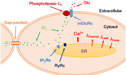Regulation with Two Different Types When an action potential reaches the pre-synaptic terminal, a large quantity of Glu will be released into the synaptic cleft. These molecules will diffuse and act on metabotropic glutamate receptors (mGluRs) which are located at adjacent branch microdomains, evoking the production of a fix amount of IP 3 [19]. This process is schematically illustrated in the upper part of Fig. 2. The concentration of IP 3 within astrocytes is believed as the key factor to evoke the elevation of intracellular calcium [9]. Moreover, as shown in Fig. 2, IP 3 is considered as the second messenger to trigger the release of Ca 2+ from endoplasmic reticulum (ER). ER can be considered as a reservoir with higher concentration of Ca 2+ than that in cytosol. A basic model in [20] has been used to describe the dynamics of Ca 2+ in cytosol due to the binding of IP 3 with IP 3 receptors ( IP 3 Rs ) in ER. There are three flows which are shown in the ER area in Fig. 2. J Leak represents the leakageflux of Ca 2+ from ER into cytosol which is directly proportional to the concentration gradient of Ca 2+ between ER and cytosol. J Pump represents the pump-flux from cytosol into ER which needs to consume energy to maintain a concentration gradient. J Channel represents the channel-flux from ER into cytosol which is generated due to the binding of IP 3 with IP 3 Rs . The elevated concentration of Ca 2+ in cytosol will further increase the open probability of IP 3 Rs and ryanodine receptors (RyRs) [21], comprising of the mechanism known as Calcium-Induced Calcium-Release (CICR). Nevertheless, excessive concentration of Ca 2+ in cytosol will bring down the open probability of IP 3 Rs and RyRs, and the pumpflux J Pump will become the main factor until a concentration gradient is re-established. Calcium waves can propagate between astrocytes to incur calcium oscillations [22]. There are many studies trying to describe and model the properties of the gap-junction between various astrocytes [23], as illustrated in Fig. 2. A large number of observations indicate that the gap-junction between astrocytes has a smaller conductance for Ca 2+ , but a larger one for IP 3 [24]. Therefore, the above-mentioned IP 3 is the main factor to promote the propagation of calcium waves between astrocytes. Besides, the activation of phospholipase C δ is also required for the propagation of calcium waves [24]. An intuitive map of the transient calcium elevation resulting from IP 3 in or between astrocytes is generalized in Fig. 2. On the other hand, neuroscience experiments have expressed different characteristics of Ca 2+ between soma and microdomains. Typically, calcium elevations occurring in the microdomains are much more frequent and transient than those in the soma [25]. Researchers in [26] indicated that there should be Transient Receptor Potential Ankyrin type 1 (TRPA1) or receptor-gated Ca 2+ -permeable ions channels in the astrocyte membrane, through which Ca 2+ could flux into the cell from the extracellular matrix. Recent studies indicate Fig. 1. An intuitive diagram of the tripartite synapse. <details> <summary>Image 1 Details</summary>  ### Visual Description ## Biological Neuron Diagram: Neuronal Structure and Synaptic Transmission ### Overview The image is a detailed biological diagram illustrating the structure of a neuron, its components, and the process of synaptic transmission. It includes labeled parts of a neuron (e.g., soma, dendrite, axon), glial cells (oligodendrocyte, microglia, astrocyte), and a zoomed-in inset detailing synaptic mechanisms. Colors are used to differentiate cell types and processes (e.g., blue for neuron structures, yellow for oligodendrocytes, pink for microglia). --- ### Components/Axes #### Labels and Elements: 1. **Neuron Components**: - **Soma**: Cell body of the neuron. - **Dendrite**: Branched extensions receiving signals. - **Axon**: Long projection transmitting signals. - **Myelin**: Insulating sheath around the axon (produced by oligodendrocytes). - **Axon Terminals**: Endpoints releasing neurotransmitters. - **Oligodendrocyte**: Glial cell myelinating axons (yellow). - **Microglia**: Immune cells (pink star-shaped). - **Astrocyte**: Star-shaped glial cell supporting synapses (orange). 2. **Synaptic Transmission Inset**: - **Pre-synapse**: Contains vesicles with neurotransmitters (e.g., glutamate, GABA). - **Post-synapse**: Includes ion channels (AMPA, NMDA receptors) and calcium waves. - **Calcium Waves**: Triggered by IP₃ signaling, leading to exocytosis. - **Gap-junction**: Direct communication between astrocytes (orange). 3. **Key Processes**: - **Action Potential**: Depolarization wave along the axon. - **Exocytosis**: Release of neurotransmitters (e.g., glutamate) into the synaptic cleft. - **Ion Channels**: mGluR (metabotropic glutamate receptor), AMPA, NMDA (ionotropic receptors). - **Second Messenger System**: IP₃ (inositol trisphosphate) and Ca²⁺ (calcium ions) signaling. --- ### Detailed Analysis #### Neuron Structure: - **Soma**: Central hub for integrating signals. - **Dendrites**: Receive synaptic inputs; branched structure increases surface area. - **Axon**: Conducts electrical impulses away from the soma. Myelinated axons (insulated by oligodendrocytes) enable faster signal propagation. - **Axon Terminals**: Release neurotransmitters (e.g., glutamate) into the synaptic cleft via exocytosis. #### Synaptic Transmission (Inset): 1. **Pre-synaptic Events**: - Action potential arrives at the axon terminal. - Voltage-gated Ca²⁺ channels open, allowing Ca²⁺ influx. - Ca²⁺ binds to sensors, triggering vesicle fusion with the membrane (exocytosis). - Neurotransmitters (e.g., glutamate) are released into the synaptic cleft. 2. **Post-synaptic Events**: - Neurotransmitters bind to receptors (AMPA, NMDA, mGluR). - **AMPA Receptors**: Allow Na⁺ influx, depolarizing the post-synaptic neuron. - **NMDA Receptors**: Require both glutamate and post-synaptic depolarization to open, permitting Ca²⁺ influx. - **mGluR**: G-protein-coupled receptors initiating second messenger pathways (e.g., IP₃ production). - **Calcium Waves**: IP₃ triggers Ca²⁺ release from intracellular stores, amplifying signaling. 3. **Glial Cell Roles**: - **Oligodendrocytes**: Myelinate axons, increasing conduction speed. - **Astrocytes**: Maintain synaptic homeostasis via gap-junctional communication and uptake of neurotransmitters. - **Microglia**: Monitor neuronal health and respond to damage/inflammation. --- ### Key Observations 1. **Signal Propagation**: The neuron’s structure (dendrites → axon → terminals) ensures unidirectional signal flow. 2. **Synaptic Complexity**: Multiple receptor types (AMPA, NMDA, mGluR) allow diverse post-synaptic responses. 3. **Glial Integration**: Astrocytes and oligodendrocytes are critical for synaptic function and myelination. 4. **Calcium Dynamics**: Ca²⁺ acts as a key second messenger, linking extracellular signals to intracellular responses. --- ### Interpretation This diagram highlights the neuron as a highly specialized cell for electrical and chemical signaling. The interplay between neurons and glial cells (oligodendrocytes, astrocytes, microglia) underscores the complexity of neural networks. The synaptic transmission process, involving Ca²⁺-dependent exocytosis and receptor-mediated signaling, demonstrates how neurons integrate and propagate information. The inset’s focus on ion channels and second messengers (e.g., IP₃) emphasizes the molecular precision required for synaptic plasticity and learning. Notably, the absence of numerical data suggests this is a conceptual model rather than a quantitative analysis, prioritizing structural and functional relationships over measurable metrics. </details> Fig. 2. The transient calcium elevation resulting from IP 3 . <details> <summary>Image 2 Details</summary>  ### Visual Description ## Diagram: Intracellular Signaling Pathway and Calcium Dynamics ### Overview This diagram illustrates a cellular signaling pathway involving extracellular glutamate (Glu), metabotropic glutamate receptors (mGluRs), phospholipase C8 (PLC8), inositol trisphosphate (IP3), calcium ions (Ca²⁺), and their regulation via the endoplasmic reticulum (ER), gap junctions, and ion channels/pumps. The diagram emphasizes spatial relationships between membrane-bound receptors, intracellular messengers, and organelles. ### Components/Axes - **Key Labels**: - **Phospholipase C8 (PLC8)**: Red oval near the top, extracellular side of the membrane. - **Glu (Glutamate)**: Extracellular space, labeled with red dots. - **mGluRs (Metabotropic Glutamate Receptors)**: Blue ovals on the plasma membrane. - **IP3 (Inositol Trisphosphate)**: Green dots diffusing from mGluRs toward the ER. - **Ca²⁺ (Calcium Ions)**: Red upward arrow from the ER lumen. - **J_Channel, J_Leak, J_Pump**: Red arrows indicating ion flux (channel, leak, pump). - **ER (Endoplasmic Reticulum)**: Yellow oval in the cytosol. - **IP3Rs (IP3 Receptors)**: Blue ovals on the ER membrane. - **RyRs (Ryanodine Receptors)**: Dark blue ovals on the ER membrane. - **Gap-junction**: Orange structure connecting two adjacent cells. - **Spatial Grounding**: - **Extracellular**: Top region, labeled with "Extracellular" and Glu. - **Plasma Membrane**: Central beige region with mGluRs and gap-junction. - **Cytosol**: Light orange region below the membrane. - **ER Lumen**: Yellow oval in the cytosol, labeled "ER." ### Detailed Analysis 1. **Signal Initiation**: - Extracellular Glu binds to mGluRs (blue ovals), activating PLC8 (red oval). - PLC8 hydrolyzes PIP2 to produce IP3 (green dots), which diffuses into the cytosol. 2. **Calcium Release**: - IP3 binds to IP3Rs (blue ovals) on the ER membrane, triggering Ca²⁺ release (red upward arrow). - Concurrently, RyRs (dark blue ovals) on the ER membrane may also mediate Ca²⁺ release, though their activation mechanism is not explicitly shown. 3. **Ion Regulation**: - **J_Channel**: Red upward arrow suggests Ca²⁺ influx into the cytosol. - **J_Leak**: Red downward arrow indicates passive Ca²⁺ efflux. - **J_Pump**: Red downward arrow represents active Ca²⁺ extrusion via pumps (e.g., SERCA). 4. **Gap-junction Communication**: - IP3 (green dots) propagates through the gap-junction (orange structure) to adjacent cells, enabling intercellular signaling. ### Key Observations - **Dominant Pathway**: Glu → mGluR → PLC8 → IP3 → Ca²⁺ release from ER. - **Redundancy**: Both IP3Rs and RyRs are shown as Ca²⁺ release channels, suggesting overlapping mechanisms. - **Ion Homeostasis**: J_Channel, J_Leak, and J_Pump regulate cytosolic Ca²⁺ levels, preventing toxicity. - **Spatial Organization**: ER is centrally located, emphasizing its role as a Ca²⁺ store. ### Interpretation This diagram highlights the integration of extracellular signaling (Glu) with intracellular Ca²⁺ dynamics. The activation of mGluRs by Glu initiates a cascade that mobilizes Ca²⁺ from the ER, a critical second messenger in processes like muscle contraction, neurotransmitter release, and gene expression. The gap-junction allows IP3 to propagate signals between cells, enabling synchronized responses. The inclusion of J_Channel, J_Leak, and J_Pump underscores the importance of precise Ca²⁺ regulation to maintain cellular function. Notably, the diagram does not specify temporal dynamics (e.g., Ca²⁺ transient duration), which would be critical for understanding physiological outcomes. The absence of quantitative data (e.g., IP3 concentration, Ca²⁺ flux rates) limits mechanistic insights but effectively conveys the pathway's architecture. </details> that there are actually two different types of regulations within astrocytes [27]. The short-range regulation in response to lowintensity stimulus is induced by rapid and short-term calcium elevations. The long-range regulation in response to highintensity stimulus is induced by slow and long-term calcium elevations. The former provides the regulation within the scale of several synapses locally, and Ca 2+ influx through the receptor-gated ions channels can be the main factor. The latter provides the regulation among different astrocytes with the propagation of calcium waves through the gap-junction, and IP 3 can be the main factor. In this paper, we focus our attention on the short-range regulation. ## C. Astrocytes as Regulation Networks Astrocytes occupy a fundamental position in the synaptic activity. It is suggested that the efficiency of synaptic transmission through the pre-synaptic terminal will be greatly decreased without the calcium signal [10]. The microdomain with elevated calcium will generate an effect for the wrapped synapse. Many researchers tried to decode the calcium signal [28] [19]. Receptors on the membrane of post-synaptic terminal have low affinity. But the interaction between synapses and astrocytes is granted by receptors with high affinity and slow TABLE I THE MAIN SYMBOLS AND ACRONYMS. | Acronym | Description | |--------------------------------------------------------------|---------------------------------------------------------------------------------------------------------------------------------------------------------------------------------------------------------------------------------------------------------------------------------------------------------------------------------------------------------------| | CNS Glu IP 3 ER IP 3 Rs RyRs CICR mGluRs AMPA NMDA TRPA1 SOM | Central Nervous System Glutamate Inositol-1,4,5-triphospate Endoplasmic Reticulum Inositol-1,4,5-triphospate receptors Ryanodine receptors Calcium Induced Calcium Release Metabotropic glutamate receptors α -Amino-3-hydroxy-5methy1-4-isoxazolepropionic acid N-methil-D-aspartic acid Transient Receptor Potential Ankyrin type 1 Self-Organizing Mapping | desensitization. It means that the influence from synapses and astrocytes will not disappear immediately. 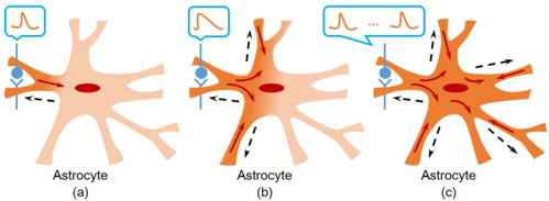In general, the arriving time of consequent action potentials at a certain synapse can be regarded as a discrete-time pulse sequence. Each of them can change the synaptic state into excitatory or inhibitory. The synaptic state change will generate calcium elevations in surrounding microdomains which will provide feedback in return. The synapse will gradually recover to its original state until the arrival of the next action potential. In this situation, the duration of the elevation depends on the length of the arriving time interval, and a shorter one will produce a longer duration. Therefore, the level of synaptic activities can be measured by the level of calcium elevations. Researchers in [8] found that increasing the level of synaptic activities would lead Ca 2+ diffusing into the adjacent microdomains, and a persistent high level would eventually make Ca 2+ be full of the whole astrocyte, which is depicted in Fig. 3. In Fig. 3, (a) represents the response of astrocytes under low intensity stimulus. The red solid arrow represents the diffusion direction of Ca 2+ while the black dotted arrow represents the feedback effect. Fig. 3 (b) is the intermediate result of increasing the intensity of stimulus. Fig. 3 (c) shows the final diffusion effect caused from a synapse which is stimulated by consequent action potentials. Fig. 3. Different levels of calcium elevations caused by different levels of synaptic activities. <details> <summary>Image 3 Details</summary>  ### Visual Description ## Diagram: Astrocyte Structure and Signaling Dynamics ### Overview The image is a three-panel diagram illustrating astrocytes (a type of glial cell) with varying structural and functional characteristics. Each panel highlights differences in dendritic processes, signaling activity, and interaction with neurons. The diagram uses color-coded elements to distinguish components and directional arrows to indicate flow or interaction. --- ### Components/Axes 1. **Panels**: - **(a)**: Basic astrocyte structure with minimal dendritic branching. - **(b)**: Intermediate astrocyte with increased dendritic complexity. - **(c)**: Advanced astrocyte with extensive dendritic branching and multiple signaling nodes. 2. **Key Elements**: - **Astrocyte Cell Body**: Red oval (central structure). - **Dendritic Processes**: Orange branches extending from the cell body. - **Neuron**: Blue circle (connected to astrocytes via dashed arrows). - **Speech Bubbles**: Represent signaling activity (peaks labeled "Signal 1," "Signal 2," etc.). - **Arrows**: Dashed black arrows indicate directional flow (e.g., neurotransmitter release, ion flux). 3. **Legend**: - **Blue**: Neuron. - **Red**: Astrocyte cell body. - **Orange**: Dendritic processes. --- ### Detailed Analysis - **Panel (a)**: - Single dendritic branch with no labeled signaling activity. - One dashed arrow connects the neuron to the astrocyte. - Speech bubble shows a single peak ("Signal 1"), suggesting minimal or baseline signaling. - **Panel (b)**: - Two dendritic branches with moderate branching. - Two dashed arrows connect the neuron to the astrocyte. - Speech bubble shows two peaks ("Signal 1" and "Signal 2"), indicating increased signaling activity. - **Panel (c)**: - Five dendritic branches with extensive branching. - Three dashed arrows connect the neuron to the astrocyte. - Speech bubble shows three peaks ("Signal 1," "Signal 2," "Signal 3"), representing heightened or multiplexed signaling. - **Color Consistency**: - All panels use the same color coding (blue neuron, red cell body, orange processes), ensuring clarity in component identification. --- ### Key Observations 1. **Progressive Complexity**: Astrocytes in panels (a) to (c) show increasing dendritic complexity, correlating with higher signaling activity. 2. **Signal Correlation**: The number of peaks in speech bubbles matches the number of dashed arrows, suggesting a direct relationship between neuronal input and astrocyte signaling. 3. **Directionality**: Arrows consistently point from the neuron to the astrocyte, implying unidirectional signaling (e.g., neurotransmitter release from the neuron to the astrocyte). --- ### Interpretation The diagram illustrates how astrocytes modulate neuronal signaling through dendritic complexity. The progression from (a) to (c) suggests that: - **Dendritic Branching**: Enhances the astrocyte's capacity to receive and process signals from neurons. - **Signaling Peaks**: Represent distinct functional states (e.g., resting, activated, or modulated states) influenced by neuronal input. - **Biological Relevance**: Astrocytes may act as integrators of synaptic activity, with dendritic architecture determining their responsiveness to neuronal signals. The dashed arrows could symbolize calcium waves, neurotransmitter uptake, or ion channel activity. This model aligns with known astrocyte functions in synaptic pruning, neurotransmitter regulation, and network homeostasis. The increasing complexity in panel (c) might reflect pathological states (e.g., neurodegeneration) or adaptive responses to environmental stimuli. 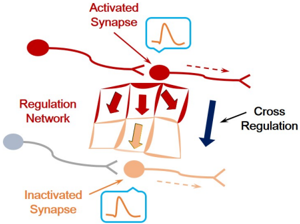</details> Many low levels of calcium elevations, which can generate the above-mentioned short-range regulations within the scale of several synapses, can jointly comprise a large state change which can be detected in the whole astrocyte. Furthermore, these calcium elevations form a Ca 2+ concentration map within astrocytes. This consideration brings about the concept that astrocytes can act as an encoder to encode the temporal properties of synaptic activities into spatial patterns. Meanwhile, astrocytes can be regarded as a spatial regulation network, in which the activity of a synapse can influence the states of other synapses not only in the adjacent area, but also in the distant regions with the help of calcium waves. As described in Fig. 4, this regulation network can provide a cross regulation for nervous system. Different from the nerve conduction, synapses by means of the spatial regulation network of astrocytes can activate other neighbor neurons between which there is no direct connection. Fig. 4. A cross regulation provided by astrocytes for nervous system. <details> <summary>Image 4 Details</summary>  ### Visual Description ## Diagram: Synaptic Regulation Network ### Overview The diagram illustrates a synaptic regulation network involving activated and inactivated synapses, a central regulation network, and cross-regulation mechanisms. Key components include labeled synapses, directional arrows indicating interactions, and waveform annotations. ### Components/Axes - **Activated Synapse**: Red-colored synapse with a waveform (orange line in blue speech bubble) positioned at the top-left. - **Inactivated Synapse**: Orange-colored synapse with a waveform (orange line in blue speech bubble) at the bottom-left. - **Regulation Network**: Central cube-like structure with bidirectional red arrows (input/output) and a single orange arrow (feedback). - **Cross Regulation**: Blue dashed arrow connecting the activated synapse (top-right) to the inactivated synapse (bottom-right). - **Legend**: Colors correspond to components: red (activated synapse), orange (inactivated synapse), blue (cross regulation), gray (unlabeled element). ### Detailed Analysis 1. **Activated Synapse**: - Positioned at the top-left, emitting a waveform (orange line) labeled "Activated Synapse." - Red arrows point from the synapse to the regulation network, indicating activation signals. 2. **Regulation Network**: - Central cube with three red arrows (input) and one orange arrow (feedback). - Arrows suggest bidirectional communication with the activated synapse and feedback to itself. 3. **Inactivated Synapse**: - Located at the bottom-left, emitting a waveform (orange line) labeled "Inactivated Synapse." - Orange arrow points from the regulation network to the synapse, indicating inhibitory regulation. 4. **Cross Regulation**: - Blue dashed arrow connects the activated synapse (top-right) to the inactivated synapse (bottom-right), suggesting reciprocal modulation. ### Key Observations - **Bidirectional Flow**: The regulation network receives input from the activated synapse and provides feedback, while also regulating the inactivated synapse. - **Color Coding**: Red/orange arrows denote activation/inhibition, while blue represents cross-regulation. - **Waveforms**: Both synapses have identical waveform annotations, implying similar signal characteristics despite activation states. ### Interpretation The diagram models a regulatory system where: 1. **Activated synapses** drive network activity and self-regulation. 2. **Inactivated synapses** are modulated by the network, potentially stabilizing activity. 3. **Cross-regulation** introduces feedback between activation states, enabling dynamic balance. 4. The absence of numerical data suggests a conceptual framework rather than quantitative analysis. The waveforms may represent action potentials or neurotransmitter release patterns, though this is speculative without explicit labels. This network could represent neuromodulatory processes, such as synaptic plasticity or homeostatic regulation, where cross-talk between activation states maintains cellular equilibrium. </details> ## D. Stigmergy in the Brain In the hippocampal stratum radiatum, the detailed 3D reconstruction work shows that 80% synapses are coupled with the branch microdomains, and astrocytes almost completely wrap synapses which are rich in docked vesicles [29]. A large number of synapses with certain functions are coupled together through astrocytes to form a potentially collaborative nervous system. Calcium waves comprise the main method of communications between synapses which are not directly connected. Accordingly, general stigmergy can be mapped into the mechanism of cooperative interaction between synapses. 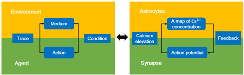In the brain's nervous system, various synapses can be regarded as different stigmergy agents, and a map of Ca 2+ concentration within astrocytes can be regarded as the medium. Action potentials can change the synaptic state into excitatory or inhibitory, which will generate different levels of calcium elevations in the corresponding microdomains. This process can be regarded as leaving traces in the medium as in general stigmergy. With the help of Ca 2+ and IP 3 , calcium waves can expand its influence throughout astrocytes. The superposition of different calcium elevations is linear, thus the effect of local traces can be integrated to adjust the whole stigmergic environment. An illustrative comparison between general stigmergy and the mechanism of stigmergic interactions between synapses and astrocytes is illustrated in Fig. 5. Fig. 5. A comparison between general stigmergy and the mechanism of stigmergic interactions between synapses and astrocytes. <details> <summary>Image 5 Details</summary>  ### Visual Description ## Diagram: Agent-Environment Interaction and Astrocyte Signaling Pathway ### Overview The image presents two interconnected diagrams illustrating (1) an agent-environment interaction model and (2) an astrocyte signaling pathway. Both diagrams use color-coded sections (yellow for "Environment"/"Astrocytes," green for "Agent"/"Synapse") and directional arrows to depict relationships between components. ### Components/Axes #### Left Diagram (Environment): - **Sections**: - **Yellow (Environment)**: Contains "Trace" (top-left) and "Medium" (center). - **Green (Agent)**: Contains "Action" (bottom-right). - **Labels**: - "Trace" → "Medium" → "Condition" → "Action" (flow sequence). - Arrows indicate bidirectional interaction between "Medium" and "Condition." #### Right Diagram (Astrocytes): - **Sections**: - **Yellow (Astrocytes)**: Contains "A map of Ca²⁺ concentration" (top-center). - **Green (Synapse)**: Contains "Action potential" (bottom-center) and "Feedback" (top-right). - **Labels**: - "A map of Ca²⁺ concentration" → "Calcium elevation" → "Action potential" → "Feedback." - Feedback loop connects "Feedback" back to "A map of Ca²⁺ concentration." ### Detailed Analysis - **Environment Diagram**: - "Trace" (likely a sensory input) interacts with "Medium" (environmental context), which influences "Condition" (external state). - "Condition" triggers "Action" (agent response). - No numerical data; focuses on abstract causal relationships. - **Astrocyte Diagram**: - "A map of Ca²⁺ concentration" (calcium ion distribution) drives "Calcium elevation" (increased intracellular Ca²⁺). - Calcium elevation generates "Action potential" (electrical signal). - "Feedback" modulates the original Ca²⁺ concentration map, suggesting homeostatic regulation. ### Key Observations 1. **Bidirectional Flow**: Both diagrams emphasize feedback loops (e.g., "Feedback" in astrocytes, bidirectional arrows in the environment model). 2. **Color Coding**: Yellow/green sections spatially separate "external" (environment/astrocyte) and "internal" (agent/synapse) components. 3. **No Numerical Data**: The diagrams are conceptual, lacking quantitative values or scales. ### Interpretation The diagrams highlight two interconnected systems: 1. **Agent-Environment Interaction**: Demonstrates how agents perceive environmental traces, process conditions, and execute actions. The feedback between "Medium" and "Condition" suggests dynamic adaptation to environmental changes. 2. **Astrocyte Signaling**: Illustrates calcium-dependent synaptic regulation. Calcium elevation in astrocytes triggers action potentials, which in turn regulate Ca²⁺ levels via feedback, emphasizing cellular homeostasis. The connection between the two diagrams implies that environmental conditions (left) may influence astrocyte signaling (right), linking external stimuli to intracellular calcium dynamics and synaptic activity. This could represent a model for how external signals modulate neural communication through glial cell activity. </details> Astrocytes can be regarded as significant medium carriers, which maintain the map of Ca 2+ concentration. Astrocytes can also provide the regulation for the involved synapses, whose implementation benefits from a large number of receptors with different types between synapses and astrocytes. This effect can be regarded as the condition provided by the medium for stigmergy agents. Besides, the concentration of Ca 2+ in astrocytes will decay with time, which comprises a negative feedback loop and provides stability for the nervous system with controlled cycles. Because of a limited range of influence, only regulations reflecting the right condition of the nervous system will superpose and have a longer duration. Through this kind of stigmergic process, astrocytes integrate the calcium elevations generated by different synapses and provide crossregulation for various individual synapses in the nervous system. ## III. 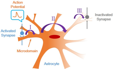STIGMERGY LEARNING MECHANISM AND MODEL Based on the aforementioned analyses, the interaction process within the scale of several synapses, which are not directly connected, can be modeled. The implementation of their interactions, which is regarded as the short-range regulation, mainly relies on the propagation of Ca 2+ throughout astrocytes. Hereinafter, we divide this process into three phases which are described in Fig. 6. The first phase which represents the generation of calcium elevation resulting from the activated synapse in the microdomain is indicated by I in Fig. 6. At first, the release of Glu due to the arriving of an action potential is modeled by [30]: $$( T _ { N e u r } ) = \frac { T _ { m a n } } { 1 + e x p ( - V _ { N e u r } ) }$$ Fig. 6. Three phases included in the interaction between synapses. They are respectively numbered by I, II and III. <details> <summary>Image 6 Details</summary>  ### Visual Description ## Biological Diagram: Neuronal Synaptic Transmission and Astrocyte Interaction ### Overview The image is a simplified biological diagram illustrating synaptic transmission between neurons and the interaction with an astrocyte. It depicts key stages of neuronal signaling, including action potential propagation, synaptic activation/inactivation, and the role of a microdomain in this process. The diagram uses color-coded elements and directional arrows to represent molecular/cellular interactions. ### Components/Axes 1. **Central Neuron**: - **Cell Body**: Orange gradient with a red oval nucleus. - **Dendrites**: Branching structures extending from the cell body. - **Axon**: Single elongated projection from the cell body. 2. **Astrocyte**: - Star-shaped cell adjacent to the neuron, labeled in blue text. 3. **Synapses**: - **Activated Synapse**: Blue-labeled structure on the left dendrite, with a waveform labeled "Action Potential." - **Inactivated Synapse**: Gray-labeled structure on the right axon terminal. 4. **Microdomain**: - Orange-labeled region on the neuron near the activated synapse. 5. **Arrows**: - Purple arrows (I, II, III) indicate directional flow: - **I**: From activated synapse to microdomain. - **II**: From microdomain to inactivated synapse. - **III**: From inactivated synapse back to the neuron. ### Detailed Analysis - **Action Potential**: Depicted as a waveform (orange line) entering the activated synapse, initiating signaling. - **Activated Synapse**: Positioned on the left dendrite, connected via arrow I to the microdomain. - **Microdomain**: Central hub for signal integration, linking activated and inactivated synapses. - **Inactivated Synapse**: Located on the right axon terminal, receiving input via arrow II and returning signal via arrow III. - **Astrocyte**: Positioned near the neuron but not directly connected by labeled pathways, suggesting a supportive or modulatory role. ### Key Observations 1. **Signal Flow**: The diagram emphasizes a unidirectional flow (I → II) from activated to inactivated synapses via the microdomain, with a feedback loop (III) from the inactivated synapse. 2. **Astrocyte Proximity**: The astrocyte is spatially adjacent to the neuron but lacks direct labeled connections, implying indirect interaction. 3. **Simplification**: The neuron is stylized (e.g., single axon, no myelin sheath), prioritizing conceptual clarity over anatomical accuracy. ### Interpretation This diagram illustrates the **synaptic transmission cycle** and highlights the **microdomain** as a critical node for signal integration. The inclusion of the astrocyte suggests its potential role in modulating synaptic activity, though the lack of direct connections implies this interaction is not explicitly detailed. The feedback loop (arrow III) may represent autoregulatory mechanisms or retrograde signaling. The absence of quantitative data (e.g., ion concentrations, timeframes) indicates the focus is on qualitative relationships rather than mechanistic precision. The diagram serves as an educational tool to visualize high-level concepts in neurobiology, emphasizing spatial organization and functional connectivity over molecular detail. </details> where [ T Neur ] is the concentration of Glu in synaptic cleft, and T max represents its maximum. V d is the voltage of dendrite in the Pinsky-Rinzel model [31]. V base and K N are parameters used to modify the sigmoid function curve. Then Glu will diffuse and act on receptors on the membrane of branch microdomain to increase the concentration of Ca 2+ : $$\frac { d ( C a ^ { 2 + } ) } { r C a } = \frac { v C a * [ T _ { Neur } ] ^ { n } } { k _ { N } C a + [ T _ { Neur } ] ^ { n } }$$ where v Ca and k Ca are regulating parameters. n is an adjusting factor. τ Ca is a decay constant. [ Ca 2+ ] ∗ represents the concentration of Ca 2+ at equilibrium in cytosol. The first item in the equation expresses the increment of Ca 2+ concentration in the microdomain. The second item indicates that the concentration also decreases with time because of the concentration gradient of Ca 2+ between cytosol and the extracellular matrix. The second phase which considers the passive diffusion of Ca 2+ from one microdomain to others is indicated by II in Fig. 6. The passive diffusion of Ca 2+ can be calculated by the Telegraph Equation [32]: $$\frac { \partial ^ { 2 } c ( x , t ) } { \partial t ^ { 2 } } + \frac { \partial c ( x , t ) } { \partial t } = r$$ where τ d is the relaxation factor accounting for a finite propagation speed. c ( x, t ) is the concentration of Ca 2+ at location x and time t . D is the diffusion coefficient. Furthermore, b ( x 0 , t ) representing the change rate of concentration at the initial point is given by [33]: $$b ( 0 , t ) = \frac { d ( b ( 0 , t ) } { d t }$$ The third phase which considers the regulation provided by astrocytes with elevated calcium for synapses is indicated by III in Fig. 6. The relationship between the concentration of Ca 2+ in the corresponding microdomain and the amplitude of slow inward currents in the pre-synaptic terminal has been used to describe the regulation [19]: $$I _ { current } = k I \theta ( n y ) y = [ C a ^ { 2 + } ] -$$ With regard to Eq. (5), there is a threshold value I th for the concentration of Ca 2+ before providing a regulation for the pre-synaptic terminal. k I is a scale factor. Θ represents the Heaviside function. A natural logarithmic function is used to describe the strength of regulation, which will generate an effect until the concentration of Ca 2+ is below a certain threshold. Therefore, this function determines a scope for the propagation of calcium waves. 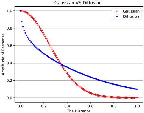Fig. 7. The strength of synaptic interaction at different distances. <details> <summary>Image 7 Details</summary>  ### Visual Description ## Line Graph: Gaussian VS Diffusion ### Overview The image is a line graph comparing two decaying response amplitudes over normalized distance. Two data series are plotted: "Gaussian" (red crosses) and "Diffusion" (blue dots). Both series show decreasing amplitude as distance increases, with a notable crossover point where the Gaussian response falls below the Diffusion response. ### Components/Axes - **Title**: "Gaussian VS Diffusion" (centered at top) - **X-axis**: "The Distance" (0.0 to 1.0 in increments of 0.2) - **Y-axis**: "Amplitude of Response" (0.0 to 1.0 in increments of 0.2) - **Legend**: Top-right corner, with red "+" for Gaussian and blue "•" for Diffusion - **Gridlines**: Horizontal and vertical, spaced at 0.2 intervals ### Detailed Analysis 1. **Gaussian Response (Red Crosses)**: - Starts at (0.0, 1.0) with maximum amplitude. - Decays rapidly, crossing the Diffusion curve at ~0.3 on the x-axis. - Reaches ~0.02 amplitude at x=1.0. - Trend: Steep initial decline, then gradual flattening. 2. **Diffusion Response (Blue Dots)**: - Starts at (0.0, 0.85) with slightly lower initial amplitude. - Decays more gradually than Gaussian. - Maintains ~0.1 amplitude at x=1.0. - Trend: Slow, linear-like decline. 3. **Crossover Point**: - Occurs at ~0.3 on the x-axis. - At this point, Gaussian amplitude ≈0.5, Diffusion ≈0.55. ### Key Observations - The Gaussian response decays faster initially but stabilizes at lower amplitudes. - The Diffusion response maintains higher amplitudes over longer distances. - Both series exhibit monotonic decay with no oscillations. ### Interpretation The graph suggests fundamentally different decay mechanisms: 1. **Gaussian Behavior**: - Rapid initial attenuation (characteristic of localized phenomena like heat diffusion in confined spaces). - Early crossover implies sensitivity to short-range interactions. 2. **Diffusion Behavior**: - Sustained amplitude retention (typical of distributed systems with gradual energy dissipation). - Linear-like decay suggests first-order diffusion processes. The crossover at ~0.3 distance units may represent a critical threshold where system dynamics shift from localized to distributed behavior. This could have implications in fields like signal processing (filter response characteristics) or physics (particle dispersion models). The stark contrast in decay rates highlights the importance of system boundary conditions in determining response profiles. </details> We can further integrate the above three phases together to describe the strength of synaptic interaction at different distances, which is represented by the Diffusion curve in Fig. 7. In Fig. 7, the Diffusion curve has been normalized to match the degree of the Gaussian function. Compared with the Gaussian function which is widely used as neighborhood function in Self-Organizing Mapping (SOM) of neural networks, the Diffusion curve has a similar downward trend. Regardless of the initial stimulus intensity, synapses with larger distances will have smaller amplitude of responses through the Diffusion process. We will take advantage of this relationship between synapses to coordinate the behaviours of stigmergy agents. 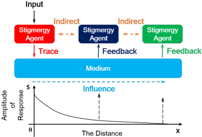More specifically, rooted in the above three interactive phases, a stigmergic learning mechanism is proposed and illustrated in Fig. 8, in which the communications between different stigmergy agents (i.e. synapses) represented by different colors are indirect. When getting a stimulus input, a stigmergy agent will leave traces (i.e. calcium elevation) which is expressed by the red solid arrow in the outside environmental medium to affect the state of other agents. As illustrated in Fig. 8, the amplitude of response for the interactive influence indicated by the blue dotted arrow is determined by the inter-synapse distance x between stigmergy agents as well as the intensity of initial stimulus s . In the nervous system, the intensity of initial stimulus is consistent with the level of synaptic activity while the synaptic distance is determined by the distance between the coupled branch microdomains within astrocytes. Environmental enrichment, which is the stimulation of the brain by its physical and social surroundings, is known to in- Fig. 8. The stigmergic learning mechanism. <details> <summary>Image 8 Details</summary>  ### Visual Description ## Diagram: Stigmergy Agent Interaction Model ### Overview The diagram illustrates a stigmergy-based interaction system where three agents (red, blue, green) influence a shared "Medium" through feedback and trace mechanisms. A graph below demonstrates how influence amplitude decays with distance from the medium. ### Components/Axes 1. **Top Section (Agents & Medium):** - **Red Agent:** Labeled "Stigmergy Agent" with a red "Trace" arrow pointing downward to the medium. - **Blue Agent:** Labeled "Stigmergy Agent" with a blue "Feedback" arrow pointing upward to the medium. - **Green Agent:** Labeled "Stigmergy Agent" with a green "Feedback" arrow pointing upward to the medium. - **Medium:** A horizontal blue rectangle labeled "Medium" at the center, receiving inputs from all agents. 2. **Bottom Section (Graph):** - **X-axis:** Labeled "The Distance" (0 to X). - **Y-axis:** Labeled "Amplitude of Response" (0 to S). - **Curve:** A dashed exponential decay curve starting at (0, S) and approaching 0 as distance increases. 3. **Arrows & Labels:** - **Red Arrow:** Connects red agent to medium, labeled "Trace." - **Blue Arrow:** Connects blue agent to medium, labeled "Feedback." - **Green Arrow:** Connects green agent to medium, labeled "Feedback." - **Dashed Line:** Connects medium to graph curve, labeled "Influence." ### Detailed Analysis - **Agent Roles:** - Red Agent: Emits "Trace" signals (unidirectional input to medium). - Blue/Green Agents: Provide "Feedback" (bidirectional interaction with medium). - **Medium Dynamics:** Acts as a shared resource modified by agents via trace/feedback loops. - **Influence Decay:** The graph shows amplitude of response decreases exponentially with distance from the medium. ### Key Observations 1. **Spatial Decay:** Influence strength (Y-axis) diminishes rapidly with increasing distance (X-axis), suggesting localized coordination. 2. **Agent Asymmetry:** Only the red agent uses "Trace," while blue/green agents use "Feedback," implying differing interaction strategies. 3. **Medium Centrality:** All agents converge on the medium, which mediates their collective influence. ### Interpretation This model represents a decentralized system where agents coordinate through environmental modification (stigmergy). The red agent's "Trace" likely represents persistent environmental changes, while blue/green agents' "Feedback" suggests real-time adjustments. The exponential decay graph implies that influence is strongest near the medium, critical for tasks requiring localized coordination (e.g., ant colony path marking). The asymmetry in agent roles may reflect specialization: one agent modifies the environment, while others respond to those modifications. The feedback loops suggest emergent self-organization, where agents adapt based on medium state changes. </details> duce the increases in synaptic and spine densities. Researchers in [34] found that great changes would present in astrocytic morphology and a large number of branch microdomains would appear in this process. Astrocytes by virtue of these emerging microdomains can coordinate synaptic activities and change the amplitude of responses between these neurons. Therefore, the inter-synapse distance adaptation between stigmergy agents in the stigmergic learning mechanism can be leveraged and well-regulated to support mutual efficient collaboration. Furthermore, a multi-agent cooperation approach is considered to take advantage of the regulation of inter-synapse distance between stigmergy agents to obtain stigmergic learning gain. Within this approach, stigmergy agents are continuously selected out for certain tasks in each turn until their common object requirements are reached. In particular, we leverage and modify the strategy proposed in [35] in each selection round: $$P _ { i , j } ( t ) = \frac { s ^ { n } _ { j } ( t ) } { s ^ { n } _ { j } ( t ) + a b _ { p } ^ { n } _ { i , j } ( t ) }$$ $$\rho _ { i , j } ( t ) = \frac { s ^ { n } _ { j } ( t ) } { s ^ { n } _ { j } ( t ) + a d r _ { i , j } ( t ) }$$ where p i,j ( t ) is the probability of i th stigmergy agent being selected for j th task. s j ( t ) is the emergency degree of j th task. α , β and n are adjusting factors. θ i,j ( t ) is the state value of i th agent for j th task. ϕ i,j ( t ) is a heuristic factor. Comparing with Eq. (6), in the modified strategy Eq. (7), ' + ' has been changed into ' ∗ ' in order to remove the asynchronous variation which will cause the jitter at steady state. After each action, the update process of s j ( t ) is modified as: $$\sum _ { S _ { j } ( t - 1 ) } ^ { R _ { j } ( t ) } r _ { m , j } ( t )$$ $$1 1 1 1 1$$ where r m,j ( t ) is the reward that m th agent obtains in j th task at time t from the outside environmental medium. R j ( t ) is the sum of all rewards at time t . T j is the expected object requirement for task j . S j ( t -1) is the set of stigmergy agents which participate in j th task at time t -1 . As more stigmergy agents participate in this task, s j ( t ) will get bigger (approach to 1) and thus provide a stimulated collaboration with higher intensity. The state value of different stigmergy agents for the same task can be different in Eq. (7). After taking an action, this state value will be updated according to the following equations: $$\theta _ { i , j } ( t ) = \theta _ { i , j } ( t - 1 ) + \alpha$$ $$\Delta \theta _ { i , j } ( t - 1 ) = p _ { i } * ( \frac { 1 } { | S _ { i } ( t - 1 ) | }$$ where ρ 1 is a scale factor. ∆ θ i,j ( t -1) can be positive or negative, which corresponds to a low or high reward respectively. According to the proposed stigmergic learning mechanism, the state change of a stigmergy agent will expand its influence to affect the state of other agents. Therefore, the state value should be further updated by: $$\theta _ { i , j } ( t ) = \theta _ { i , j } ( t ) + \Delta t$$ $$\sum _ { k \in r _ { 1 } ( t - 1 ) } D ( d _ { k , j } ( t m can be efficient$$ where ρ 2 is a scale factor. π i ( t -1) = { X k | k = i, d k,i ( t -1) < d th } . d k,i ( t -1) is the inter-synapse distance between k th and i th agent at time t -1 . d th is a threshold value for the inter-synapse distance. D ( · ) represents the interaction process which includes the above-mentioned three phases. Here we use ∆ θ k,j ( t -1) to represent the intensity of stimulus provided by k th agent for i th agent, which will be discounted by their synaptic distance. The distance between stigmergy agents, which describes the strength of synaptic interaction, can be regulated according to the feedback. Accordingly, we further put forward the following scheme to regulate the distance after each action: $$\begin{aligned} d _ { k , i } ( t ) = \{ d _ { k , i } ( t - 1 ) - f _ { g } \quad \text{if } \phi > 0 \\ &= \{ d _ { k , i } ( t - 1 ) + f _ { g } \quad \text{otherwise} \end{aligned}$$ $$t - 1 ) ( 1 5 )$$ where factor is a constant. To some extent, the distance between stigmergy agents also represents the similarity of these agents participating in the same task. Therefore, the strength of interactions will be larger if the similarity between two stigmergy agents is higher. The regulation of inter-synapse distance can adjust the strength of synaptic interactions between stigmergy agents and thus bring the systematic stigmergy learning gain. ## IV. NUMERICAL SIMULATION AND RESULTS In order to verify the effectiveness and advantages of the proposed stigmergy learning model, a number of numerical simulations with different kinds of tasks have been carried out. ## A. The Stigmergy Learning Gain In the first simulation, there is only one task to be finished. During the initialization, the distance between various neural agents is set as the median value in the range, which can represent the similarity of these agents participating in this task. The same method is also applied to the setting of the state value. A random reward is assigned to each neural agent which will not be changed during the whole simulation process. Several neural agents are allowed to take an action together as a batch. There is a fixed cost for each action which is the same for all agent individuals. Besides, an ability value is randomly assigned to each neural agent indicating the number of actions it can still take, which is also utilized as the heuristic factor in Eq. (7) and normalized to match the degree of the state value. In each turn, several neural agents are selected out according to the selection probability (Eq. (7)) as a batch to participate in the target task until the overall reward is above the object requirement. After each turn, a feedback is returned, which equals to the sum of all rewards of neural agents that are selected out in last turn. This feedback is used to regulate the distance between neural agents. The target of the simulation is to satisfy the object requirement with the maximum utility value (reward/cost). The main parameters within the simulation are shown in Table II. TABLE II THE MAIN PARAMETERS. | Item | Description | |--------------------|---------------| | Agent number | 30 | | Object requirement | 1100 | | Batch size | 5 | | Agent reward | [1 , 10] | | Agent ability | [50 , 120] | | Cost | 10 | | α | 2 | | β | 2 | | n | 2 | | ρ 1 | 0 . 001 | | ρ 2 | 1 | | factor | 0 . 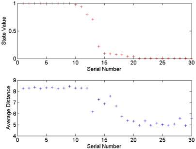5 | According to the selection probability, neural agents with higher rewards are assumed to have smaller state values and thus more likely to be selected. These neural agents will shorten the distance between those agents with the same higher rewards to form a cluster. Based on the proposed stigmergy learning model (Eq. (7) - (15)), aiming at forming a spatial neural cluster, the task is repeatedly carried out for 500 times to regulate the distance between neural agents. The state value and the average distance of neural agents are given in Fig. 9. In Fig. 9, neural agents are arranged in descending order according to the state values. Similarly, the average distance which represents the average distance value of a neural agent from all the other agents is arranged according to the corresponding order. It can be observed that the neural agents with lower state values will have smaller average distances. Therefore, a neural cluster can be automatically formed by agents with higher rewards. Members in the neural cluster have smaller distances than the others, whose stimulus resulting from the state change can thus be more easily responded. Fig. 9. The state value and the average distance of neural agents. <details> <summary>Image 9 Details</summary>  ### Visual Description ## Line Graphs: State Value and Average Distance vs. Serial Number ### Overview The image contains two vertically stacked line graphs. The top graph plots "State Value" (y-axis) against "Serial Number" (x-axis), while the bottom graph plots "Average Distance" (y-axis) against the same "Serial Number" (x-axis). Both graphs use plus markers (+) to represent data points. ### Components/Axes - **X-axis (Serial Number)**: - Range: 0 to 30 (integer increments). - Label: "Serial Number" (black text). - **Top Graph (State Value)**: - Y-axis: "State Value" (black text). - Scale: 0 to 1 (linear, with ticks at 0, 0.5, 1). - Data Points: Red plus markers (+). - **Bottom Graph (Average Distance)**: - Y-axis: "Average Distance" (black text). - Scale: 4 to 9 (linear, with ticks at 4, 5, 6, 7, 8, 9). - Data Points: Blue plus markers (+). ### Detailed Analysis #### Top Graph (State Value): - **Trend**: - Serial Numbers 0–10: State Value remains constant at 1. - Serial Numbers 11–15: Gradual decline from 1 to ~0.5. - Serial Numbers 16–20: Sharp drop to 0. - Serial Numbers 21–30: State Value remains at 0. - **Key Data Points**: - Serial 0: 1.0 - Serial 10: 1.0 - Serial 15: ~0.5 - Serial 20: 0.0 #### Bottom Graph (Average Distance): - **Trend**: - Serial Numbers 0–10: Average Distance remains constant at ~8. - Serial Numbers 11–15: Gradual decline from ~8 to ~6. - Serial Numbers 16–20: Fluctuates between ~5 and ~6. - Serial Numbers 21–30: Slight increase to ~5.5–6. - **Key Data Points**: - Serial 0: ~8.0 - Serial 10: ~8.0 - Serial 15: ~6.0 - Serial 20: ~5.5 - Serial 30: ~5.5 ### Key Observations 1. **State Value**: - Drops to 0 by Serial 20, suggesting a binary or threshold-based behavior (e.g., "on/off" state). - Sharp decline between Serials 15–20 indicates a critical transition. 2. **Average Distance**: - Correlates inversely with State Value: both decrease as Serial Number increases. - Post-Serial 20 fluctuations suggest variability in distance measurements after the State Value stabilizes at 0. 3. **Synchronization**: - Both graphs share the same x-axis (Serial Number), implying a shared temporal or sequential context. ### Interpretation - **State Value**: The abrupt drop to 0 at Serial 20 suggests a system reset, failure, or completion of a process. The prior gradual decline (Serials 10–15) may indicate degradation or preparation for this transition. - **Average Distance**: The inverse relationship with State Value implies that the "distance" metric (e.g., physical, computational, or abstract) decreases as the system transitions from an active state (State Value = 1) to an inactive state (State Value = 0). Post-Serial 20 fluctuations could reflect residual activity or measurement noise. - **Critical Threshold**: Serial 20 marks a pivotal point where both metrics stabilize, suggesting a system boundary or operational limit. ### Spatial Grounding - **Legend**: No explicit legend is present. Colors (red for State Value, blue for Average Distance) are inferred from marker colors and axis labels. - **Positioning**: - Top graph: State Value (red) occupies the upper half. - Bottom graph: Average Distance (blue) occupies the lower half. - Both share the same x-axis (Serial Number), emphasizing their sequential relationship. ### Content Details - **State Value**: - Red markers: - Serials 0–10: 1.0 (exact). - Serials 11–15: ~0.5–1.0 (approximate). - Serials 16–20: 0.0 (exact). - **Average Distance**: - Blue markers: - Serials 0–10: ~8.0 (exact). - Serials 11–15: ~6.0–8.0 (approximate). - Serials 16–20: ~5.0–6.0 (approximate). - Serials 21–30: ~5.5–6.0 (approximate). ### Uncertainties - Exact values for Serials 11–15 (State Value) and 16–20 (Average Distance) are approximate due to marker clustering. - Post-Serial 20 fluctuations in Average Distance lack clear numerical precision. ### Final Notes The graphs likely represent a system’s operational lifecycle, where State Value acts as a binary indicator and Average Distance reflects a secondary metric tied to system activity. The absence of a legend necessitates reliance on color coding and axis labels for interpretation. 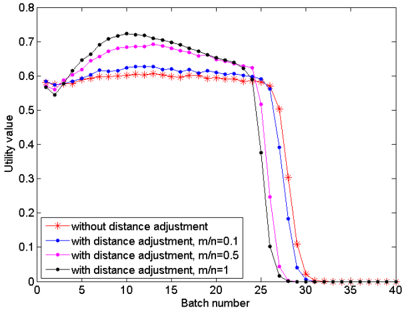</details> The obtained neural cluster can be used to generate the stigmergy learning gain. We have compared the utility value of each batch with that in general stigmergy, in which the distance adjustment between stigmergic agents as well as the formation of the neural cluster are not taken into account. The comparison results are provided in Fig. 10. In Fig. 10, the curve without distance adjustment represents the utility value of the traditional stigmergy mechanism while the curves with distance adjustment represent the utility values of the proposed stigmergy learning model. m in Fig. 10 represents the maximum of ∆ θ i,j ( t ) while n represents the maximum of ∆ θ i,j ( t ) . Because of the limitation of the ability value, the last few rounds in each scheme have to adopt neural agents with lower rewards, which cause the decline of each curve in the end. With the existence of the regulated distance, the task is started with higher efficiency and completed earlier. Accordingly, neural agents with higher rewards are more easily selected in the task and further activate those with the same higher rewards because of the neural clustering merit. Therefore, as a key in the proposed stigmergy learning model, the Fig. 10. The system gain provided by the regulated distance between neural agents. <details> <summary>Image 10 Details</summary>  ### Visual Description ## Line Graph: Utility Value vs Batch Number ### Overview The image depicts a line graph comparing utility values across 40 batches for four scenarios: "without distance adjustment" and three configurations with distance adjustment (m/n = 0.1, 0.5, 1.0). Utility values range from 0 to 0.8, with distinct trends observed for each configuration. ### Components/Axes - **X-axis (Batch number)**: Integers from 0 to 40, labeled "Batch number." - **Y-axis (Utility value)**: Scale from 0 to 0.8, labeled "Utility value." - **Legend**: Located at the bottom-left corner, with four entries: - Red stars: "without distance adjustment" - Blue circles: "with distance adjustment, m/n=0.1" - Magenta diamonds: "with distance adjustment, m/n=0.5" - Black squares: "with distance adjustment, m/n=1" - **Line styles**: Each configuration uses a unique color and marker type. ### Detailed Analysis 1. **Without distance adjustment (red stars)**: - Utility value remains stable (~0.55–0.6) until batch 25. - Sharp decline to ~0.05 by batch 30, then plateaus near 0. 2. **With distance adjustment, m/n=0.1 (blue circles)**: - Utility value starts at ~0.55, peaks at ~0.62 by batch 10. - Gradual decline to ~0.4 by batch 25, then steep drop to ~0.05 by batch 30. 3. **With distance adjustment, m/n=0.5 (magenta diamonds)**: - Utility value starts at ~0.58, peaks at ~0.68 by batch 10. - Steeper decline than m/n=0.1, reaching ~0.3 by batch 25 and ~0.05 by batch 30. 4. **With distance adjustment, m/n=1 (black squares)**: - Utility value starts at ~0.57, peaks at ~0.72 by batch 10. - Most pronounced decline, dropping to ~0.2 by batch 25 and ~0.05 by batch 30. ### Key Observations - **Peak utility**: All configurations with distance adjustment (m/n=0.1, 0.5, 1.0) exhibit higher initial utility values (~0.55–0.72) compared to the "without adjustment" baseline (~0.55–0.6). - **Decline pattern**: - The "without adjustment" line shows a delayed but abrupt collapse after batch 25. - Configurations with higher m/n values (e.g., m/n=1) experience steeper declines post-batch 25. - Lower m/n values (e.g., m/n=0.1) exhibit more gradual declines but still fall below the baseline by batch 30. - **Stability**: The "without adjustment" line remains stable until batch 25, suggesting distance adjustment introduces sensitivity to batch progression. ### Interpretation The data suggests that distance adjustment parameters (m/n) significantly impact utility value dynamics: - **Higher m/n values** (e.g., 1.0) correlate with higher peak utility but accelerated degradation over batches. - **Lower m/n values** (e.g., 0.1) balance peak utility and gradual decline, potentially indicating a trade-off between initial performance and long-term stability. - The "without adjustment" baseline demonstrates resilience until batch 25, after which utility collapses, implying that distance adjustment may introduce vulnerabilities in later stages. This pattern could reflect system optimization trade-offs, where distance adjustment improves early performance but destabilizes the system over time. Further investigation into the underlying mechanisms (e.g., parameter definitions, batch-specific stressors) is warranted to validate these hypotheses. </details> regulation of distance between various neural agents through spatial clustering can bring expected gain for the learning system. ## B. The Impact of Distance Regulation Different from the first simulation, the aim of the second simulation is to test if we can adjust current states of neural agents to converge to the target pattern (e.g. a target picture of Arabic numerals). The selection of neural agents is different with that in the first simulation, namely, 120 agents are randomly selected out to form a neural group in each turn. 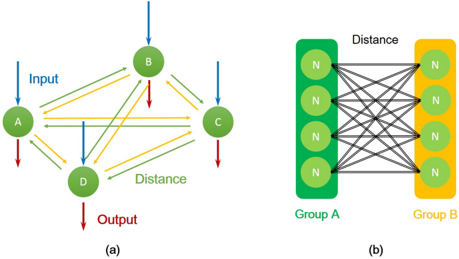The current state of each neural agent is redefined by: $$y _ { j } = \theta ( \sum _ { i = 1 } ^ { n } v _ { i } * D ( d _ { i , j } )$$ where base is a constant. Θ represents the Heaviside function. v i represents the input of i th agent. y j represents the output of j th agent. y j = 1 means that the current state of j th agent is excitatory while y j = 0 means that the current state of j th agent is inhibitory. Self-feedback is not considered here. The relationship between neural agents is illustrated in Fig. 11 (a), in which distances between neural agents are directed. Regardless of the initial input, according to Eq. (16), the current state of a neural agent is determined by the distance from the other agents. Fig. 11. The relationship between neural agents. <details> <summary>Image 11 Details</summary>  ### Visual Description ## Diagram Analysis: Network and Bipartite Graph Structures ### Overview The image contains two distinct diagrams labeled (a) and (b). Diagram (a) depicts a directed network with labeled nodes and colored arrows, while diagram (b) illustrates a bipartite graph with grouped nodes and labeled connections. Both diagrams emphasize relationships ("Distance") and directional flows ("Input"/"Output"). --- ### Components/Axes #### Diagram (a) - **Nodes**: Labeled A, B, C, D (green circles). - **Arrows**: - **Blue (Input)**: From A and C to B. - **Red (Output)**: From B and D to a terminal node. - **Yellow/Green (Distance)**: Bidirectional connections between A-B, B-C, C-D, and A-D. - **Labels**: "Input" (top-left), "Output" (bottom-right), "Distance" (center-right). #### Diagram (b) - **Groups**: - **Group A**: Left column (green nodes labeled N). - **Group B**: Right column (yellow nodes labeled N). - **Connections**: Black lines labeled "Distance" between all nodes in Group A and Group B. - **Labels**: "Distance" (top-center), "Group A" (left), "Group B" (right). --- ### Detailed Analysis #### Diagram (a) - **Flow Structure**: - Input nodes (A, C) feed into node B. - Node B and D propagate signals to the Output terminal. - Distance connections form a cyclic network (A-B-C-D-A). - **Color Coding**: - Input (blue) and Output (red) arrows are unidirectional. - Distance (yellow/green) arrows are bidirectional, suggesting mutual influence. #### Diagram (b) - **Bipartite Graph**: - Complete connections between Group A and Group B (all N×N links). - Uniform "Distance" labels imply pairwise metrics between groups. - **Node Uniformity**: - All nodes in each group are identical (labeled N), suggesting homogeneity within groups. --- ### Key Observations 1. **Diagram (a)**: - Node B acts as a central hub for input processing. - Output is generated via B and D, indicating redundancy or parallel pathways. - Distance connections form a closed loop, possibly representing feedback or interdependence. 2. **Diagram (b)**: - All-to-all connections between groups suggest exhaustive comparison (e.g., similarity, dissimilarity). - Absence of self-connections within groups implies no intra-group distance metrics. --- ### Interpretation - **Diagram (a)** resembles a simplified neural network or decision-making system: - Input nodes (A, C) contribute to a central processor (B). - Output is derived from B and D, with distance metrics governing node interactions. - The cyclic distance connections may model feedback loops or systemic stability. - **Diagram (b)** aligns with clustering or similarity analysis: - Groups A and B could represent distinct clusters or categories. - The "Distance" labels imply a matrix of pairwise comparisons, critical for tasks like anomaly detection or classification. - **Shared Themes**: - Both diagrams emphasize relational metrics ("Distance") over absolute values. - Directionality in (a) contrasts with bidirectionality in (b), reflecting different modeling approaches (sequential vs. comparative). --- ### Limitations - No numerical data or scales are provided, limiting quantitative analysis. - Node labels (A, B, C, D, N) are abstract; real-world interpretation requires contextual mapping. </details> In each turn, all neural agents will be given a unit input to determine the current states of neural agents in the group. These states can be further used to calculate the feedback which equals to the sum of all rewards of neural agents in the group. The reward for each state of neural agent is provided in Table III. In Table III, the value of a pixel refers to the binary value in the original picture. The size of the original picture is 28 × 28 , in which each pixel is represented by the state of a neural agent in the corresponding location. According to the selection method, different neural groups that may contain the same members are selected out in different turns. Neural agents in each group will regulate the distance to adjust their current states according to the corresponding feedback. Concretely, as shown in Fig. 11 (b), we compare the feedback of two neural groups in two continuous turns and change the distance between any two members in different neural groups according to the result. The distance TABLE III THE REWARD FOR EACH STATE. | state | pixel | reward | |---------|---------|----------| | 1 | 1 | 0 | | 1 | 0 | -1 | | 0 | 1 | +1 | | 0 | 0 | 0 | from neural agents in the group with larger feedback to the others in the group with smaller one will increase a constant in each turn. As mentioned before, the distance between neural agents describes the strength of interactions between them and a shorter distance indicates a higher strength. In this way, neural agents which should be excitatory for the target pattern will get shorter distances and be more easily activated. Fig. 12. The learning process of the sitgmergy learning system. <details> <summary>Image 12 Details</summary>  ### Visual Description ## Grid Visualization: Pixel Density vs. Delta Values ### Overview The image displays eight black-and-white grids arranged in a 2x4 matrix. Each grid represents a different pixel density (n) with corresponding delta values (d̄). The grids transition from sparse to dense pixel distributions, with numerical labels indicating the number of pixels (n) and calculated delta values (d̄) beneath each grid. ### Components/Axes - **Grid Layout**: Two rows of four grids each. - **Labels**: Each grid has a label below it specifying: - **n**: Number of pixels (e.g., "n=0", "n=800", ..., "n=7000"). - **d̄**: Delta value (e.g., "d̄=0.5008", "d̄=0.4925", ..., "d̄=0.4815"). - **No Axes/Legends**: The image lacks explicit axes, scales, or legends beyond the grid labels. ### Detailed Analysis 1. **Top Row (n=0 to n=2400)**: - **n=0**: Empty grid, d̄=0.5008. - **n=800**: Sparse pixel distribution, d̄=0.4925. - **n=1600**: Moderate density, d̄=0.4841. - **n=2400**: Dense but fragmented, d̄=0.4808. 2. **Bottom Row (n=4000 to n=7000)**: - **n=4000**: High density with gaps, d̄=0.5171 (outlier). - **n=5000**: More cohesive, d̄=0.5035. - **n=6000**: Near-complete coverage, d̄=0.4921. - **n=7000**: Fully formed digit "8", d̄=0.4815. ### Key Observations - **General Trend**: Delta values (d̄) decrease as pixel count (n) increases, suggesting improved efficiency or stability with higher densities. - **Outlier**: The grid at n=4000 has a higher d̄ (0.5171) than its neighbors, indicating a potential anomaly or inefficiency at this density. - **Digit Formation**: The final grid (n=7000) clearly represents the digit "8", while earlier grids show progressive formation of this shape. ### Interpretation The data suggests a relationship between pixel density and a metric (d̄) that improves (decreases) as more pixels are added. The outlier at n=4000 may reflect a transitional phase where increased density introduces complexity before stabilizing. The formation of the digit "8" at n=7000 implies the grids represent stages in rendering or reconstructing a specific pattern, with d̄ possibly measuring reconstruction accuracy or computational efficiency. The initial high d̄ at n=0 (0.5008) and gradual decline to 0.4815 at n=7000 highlight a systematic improvement in the underlying process as data complexity increases. </details> The relevant simulation results are shown in Fig. 12. n is the number of learning iterations. d represents the corresponding average distance from the others to the neural agent which should be excitatory at each iteration step. Each picture in Fig. 12 describes the current states of all neural agents during the learning process. White points in each picture indicate Fig. 13. The utility value during the stigmergy learning process. 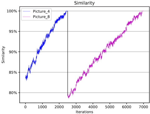<details> <summary>Image 13 Details</summary>  ### Visual Description ## Line Graph: Similarity Analysis of Picture_4 and Picture_8 ### Overview The image is a line graph comparing the similarity scores of two datasets, "Picture_4" (blue line) and "Picture_8" (pink line), across 7,000 iterations. Similarity is measured on the y-axis (80%–100%), while iterations are plotted on the x-axis (0–7,000). Both lines show upward trends, but with distinct trajectories. --- ### Components/Axes - **Title**: "Similarity" (centered at the top). - **X-axis**: - Label: "Iterations" (black text). - Scale: 0 to 7,000 in increments of 1,000. - **Y-axis**: - Label: "Similarity" (black text). - Scale: 80% to 100% in 5% increments. - **Legend**: - Position: Top-left corner. - Entries: - Blue line: "Picture_4". - Pink line: "Picture_8". - **Additional Elements**: - Vertical dashed line at ~3,000 iterations (black, unlabeled). --- ### Detailed Analysis 1. **Picture_4 (Blue Line)**: - **Starting Point**: ~83% similarity at 0 iterations. - **Trend**: Steady, linear increase with minor fluctuations. - **Key Milestones**: - Reaches ~95% similarity by ~2,000 iterations. - Achieves 100% similarity by ~2,000 iterations (plateaus). 2. **Picture_8 (Pink Line)**: - **Starting Point**: ~79% similarity at ~3,000 iterations (delayed start). - **Trend**: Gradual increase with sharper fluctuations early on. - **Key Milestones**: - Reaches ~95% similarity by ~6,000 iterations. - Achieves 100% similarity by ~7,000 iterations. 3. **Vertical Dashed Line**: - Positioned at ~3,000 iterations. - Aligns with the start of Picture_8's data, suggesting a potential phase shift or initialization point. --- ### Key Observations - **Convergence Speed**: Picture_4 achieves maximum similarity (100%) significantly faster (~2,000 iterations) than Picture_8 (~7,000 iterations). - **Initial Delay**: Picture_8's data begins at ~3,000 iterations, implying a lag or preprocessing phase. - **Fluctuations**: Picture_8 exhibits more variability in its early growth phase compared to Picture_4's smoother trajectory. - **Vertical Line Significance**: The dashed line at 3,000 iterations may mark a critical threshold (e.g., algorithm activation, data loading). --- ### Interpretation The graph demonstrates that Picture_4's similarity metric converges rapidly and stably, while Picture_8 experiences a delayed start and slower, noisier progression. The vertical dashed line at 3,000 iterations likely indicates when Picture_8's processing began, highlighting a potential inefficiency or resource constraint in its workflow. The stark difference in convergence times suggests differing algorithmic efficiencies or data complexities between the two datasets. The anomaly in Picture_8's initial dip (below 80%) could reflect transient noise or initialization artifacts. Overall, the data underscores the importance of optimizing processing pipelines to minimize delays and variability in similarity-based tasks. </details> that neural agents at those locations are excitatory while black points indicate that neural agents at those locations are inhibitory. As the number of iterations increases, the learning system gradually converges to the clear target pattern of number 4 or 8. At the same time, the average distance d decreases gradually, indicating that the average amplitude of response of these neural agents increases gradually. After n = 2400 , the learning system starts to change its regulation and to express another target pattern of number 8. As before, the sitgmergy learning system finally learns the target pattern of number 8 after 7000 iterations. Fig. 13 shows the similarity between the original target picture and the one formed by the learning system during the whole process. The above results have proved that the proposed stigmergy learning system can be adjusted to learn the target patterns, which is accomplished by activating the relevant sets of neural agents. Regardless of the initial stimulus, the activation of a neural agent is determined by the distance to other neuron individuals. Note that the distance represents the strength of interactions between neural agents which will be activated more easily with shorter distances from the others. In summary, the regulation of inter-synapse distance plays an important role for the cooperation of neural agents in the stigmergy learning mechanism. ## V. CONCLUSIONS Stigmergy phenomena are widely discovered in natural colonies and perform well through the way of collective collaboration. Inspired by the new discoveries on astrocytes in synaptic transmission, we have explored and mapped stigmergy in the regulation of synaptic activities in the brain. In particular, the interaction between neural agents (synapses) is divided into three important phases and a stigmergic learning system model has been put forward. We have found that the regulation of distance between neural agents plays an important role in the proposed model. The well-regulated distance between neural agents can bring gain for the system and help to learn the target patterns. Its importance has been verified in two different simulations. Please note that the interaction between synapses within a certain range has been regarded as the short-range regulation. But for the long-range regulation, the participation of IP 3 must be taken into account, which will be our future research direction. ## REFERENCES - [1] P. Grass, 'La reconstruction du nid et les coordinations inter -individuelles chez Bellicositermes natalis et Cubitermes sp. La thorie de la stigmergie,' Insectes Sociaux , vol. 6, no. 1, pp. 41-80, 1959. - [2] U. Gllner, 'Grass, PierreP.: Fondation des Socit Construction. Termitologia. 2. 624 S., 452 Fig., 28 Tab., Masson, Paris, New York, Barcelona, Milan, Mexico, Sao Paulo, 1984,' Deutsche Entomologische Zeitschrift , vol. 32, no. 45, pp. 379-379, 1985. - [3] I. F. Informatik, H. Dipl.-Inf, and S. A. Br, 'Return From The Ant Synthetic Ecosystems For Manufacturing Control,' in PhD Thesis , 2000. - [4] F. Heylighen, 'Stigmergy as a generic mechanism for coordination: definition, varieties and aspects,' 2011. - [5] M. Dorigo, G. D. Caro, and L. M. Gambardella, 'Ant algorithm for discrete optimization,' Artificial Life , vol. 5, no. 2, pp. 137 - 172, 1999. - [6] I. Kassabalidis, M. A. Elsharkawi, R. J. Marks, P. Arabshahi, and A. A. Gray, 'Swarm Intelligence for Routing in Communication Networks,' IEEE Globecom , vol. 6, pp. 3613-3617, vol. 6, 2001. - [7] P. G. Haydon and G. Carmignoto, 'Astrocyte Control of Synaptic Transmission and Neurovascular Coupling,' Physiological Reviews , vol. 86, no. 3, pp. 1009-1031, 2006. - [8] A. Araque, G. Carmignoto, P. G. Haydon, S. H. Oliet, R. Robitaille, and A. Volterra, 'Gliotransmitters travel in time and space.' Neuron , vol. 81, no. 4, pp. 728-739, 2014. - [9] F. Mesiti, P. A. Floor, and I. Balasingham, 'Astrocyte to Neuron Communication Channels With Applications,' IEEE Transactions on Molecular, Biological and Multi-Scale Communications , vol. 1, no. 2, pp. 164-175, 2015. - [10] M. Navarrete and A. Araque, 'Basal synaptic transmission: astrocytes rule!' Cell , vol. 146, no. 5, pp. 675-7, 2011. - [11] L. Correia, A. M. Sebastio, and P. Santana, 'On the role of stigmergy in cognition,' Progress in Artificial Intelligence , pp. 1-8, 2017. - [12] D. Erny, A. L. H. de Angelis, and M. Prinz, 'Communicating systems in the body: how microbiota and microglia cooperate,' Immunology , vol. 150, no. 1, 2016. - [13] R. M. Ransohoff, 'How neuroinflammation contributes to neurodegeneration,' Science , vol. 353, no. 6301, p. 777, 2016. - [14] S. Pajevic, P. J. Basser, and R. D. Fields, 'Role of Myelin Plasticity in Oscillations and Synchrony of Neuronal Activity,' Neuroscience , vol. 276, no. 6, pp. 135-147, 2013. - [15] R. D. Fields, 'A new mechanism of nervous system plasticity: activitydependent myelination,' Nature Reviews Neuroscience , vol. 16, no. 12, p. 756, 2015. - [16] M. V. Sofroniew and H. V. Vinters, 'Astrocytes: biology and pathology,' Acta Neuropathologica , vol. 119, no. 1, pp. 7-35, 2010. - [17] A. Araque, V. Parpura, R. P. Sanzgiri, and P. G. Haydon, 'Tripartite synapses: glia, the unacknowledged partner,' Trends in Neurosciences , vol. 22, no. 5, p. 208, 1999. - [18] P. Bezzi and A. Volterra, 'A neuron-glia signalling network in the active brain,' Current Opinion in Neurobiology , vol. 11, no. 3, pp. 387-394, 2001. - [19] S. Nadkarni and P. Jung, 'Dressed neurons: modeling neural-glial interactions.' Physical Biology , vol. 1, no. 2, pp. 35-41, 2004. - [20] Y. X. Li and J. Rinzel, 'Equations for InsP3 receptor-mediated [Ca2+]i oscillations derived from a detailed kinetic model: a Hodgkin-Huxley like formalism,' Journal of Theoretical Biology , vol. 166, no. 4, pp. 461-73, 1994. - [21] I. Siekmann, P. Cao, J. Sneyd, and E. J. Crampin, 'Data-driven modelling of the inositol trisphosphate receptor (IPR) and its role in calcium induced calcium release (CICR),' Quantitative Biology , 2015. - [22] M. J. Berridge and A. Galione, 'Cytosolic calcium oscillators,' Faseb Journal Official Publication of the Federation of American Societies for Experimental Biology , vol. 2, no. 15, pp. 3074-82, 1988. - [23] M. Goldberg, M. D. Pitt, V. Volman, H. Berry, and E. Benjacob, 'Nonlinear Gap Junctions Enable Long-Distance Propagation of Pulsating Calcium Waves in Astrocyte Networks,' PLOS Computational Biology , vol. 6, no. 8, pp. 1-14, 2010. - [24] J. Pouilloux, 'Anti-phase calcium oscillations in astrocytes via inositol (1, 4, 5)-trisphosphate regeneration,' Cell Calcium , vol. 39, no. 3, pp. 197208, 2006. - [25] K. Kanemaru, H. Sekiya, M. Xu, K. Satoh, N. Kitajima, K. Yoshida, Y. Okubo, T. Sasaki, S. Moritoh, and H. Hasuwa, 'In vivo visualization of subtle, transient, and local activity of astrocytes using an ultrasensitive Ca(2+) indicator.' Cell Reports , vol. 8, no. 1, pp. 311-318, 2014. - [26] E. Shigetomi, X. Tong, K. Y. Kwan, D. P. Corey, and B. S. Khakh, 'TRPA1 channels regulate astrocyte resting calcium and inhibitory synapse efficacy through GAT-3,' Nature Neuroscience , vol. 15, no. 1, pp. 70-80, 2012. - [27] N. Bazargani and D. Attwell, 'Astrocyte calcium signaling: the third wave,' Nature Neuroscience , vol. 19, no. 2, pp. 182-189, 2016. - [28] P. M. De, V. Volman, H. Levine, and E. Ben-Jacob, 'Multimodal encoding in a simplified model of intracellular calcium signaling,' Cognitive Process , vol. 10, no. 1, pp. 127-127, 2009. - [29] R. Ventura and K. M. Harris, 'Three-dimensional relationships between hippocampal synapses and astrocytes.' The Journal of Neuroscience , vol. 19, no. 16, p. 6897, 1999. - [30] A. Destexhe, Z. F. Mainen, and T. J. Sejnowski, 'Synthesis of models for excitable membranes, synaptic transmission and neuromodulation using a common kinetic formalism.' Journal of Computational Neuroscience , vol. 1, no. 3, pp. 195-230, 1994. - [31] P. F. Pinsky and J. Rinzel'S, Intrinsic and Network Rhythmogenesis in a Reduced Traub Model for CA3 Neurons . Springer-Verlag New York, Inc., 1995. - [32] Y. M. Ali and L. C. Zhang, 'Relativistic heat conduction,' International Journal of Heat and Mass Transfer , vol. 48, no. 12, pp. 2397-2406, 2005. - [33] M. Pierobon and I. F. Akyildiz, 'A physical end-to-end model for molecular communication in nanonetworks,' IEEE Journal on Selected Areas in Communications , vol. 28, no. 4, pp. 602-611, 2010. - [34] G. G. Viola, L. Rodrigues, J. C. Amrico, G. Hansel, R. S. Vargas, R. Biasibetti, A. Swarowsky, C. A. Gonalves, L. L. Xavier, and M. Achaval, 'Morphological changes in hippocampal astrocytes induced by environmental enrichment in mice,' Brain Research , vol. 1274, pp. 47-54, 2009. - [35] M. Dorigo, E. Bonabeau, and G. Theraulaz, Ant Algorithms and Stigmergy . Elsevier Science Publishers B. V., 2000.