## Specification-Guided Safety Verification for Feedforward Neural Networks
Weiming Xiang ∗ , Hoang-Dung Tran ∗ , Taylor T. Johnson ∗
December 18, 2018
tions or properties of neural networks. Verifying neural networks is a hard problem, even simple properties about them have been proven NP-complete problems [2]. The difficulties mainly come from the presence of activation functions and the complex structures, making neural networks large-scale, nonlinear, non-convex and thus incomprehensible to humans.
The importance of methods of formal guarantees for neural networks has been well-recognized in literature. There exist a number of results for verification of feedforward neural networks, especially for Rectifier Linear Unit (ReLU) neural networks, and a few results are devoted to neural networks with broad classes of activation functions. Motivated to general class of neural networks such as those considered in [3], our key contribution in this paper is to develop a specificationguided method for safety verification of feedforward neural network. First, we formulate the safety verification problem in the framework of interval arithmetic, and provide a computationally efficient formula to compute output interval sets. The developed formula is able to calculate the output intervals in a fast manner. Then, analogous to other state-of-the-art verification methods, such as counterexample-guided abstraction refinement (CEGAR) [4] and property directed reachability (PDR) [5], and inspired by the Moore-Skelboe algorithm [6], a specification-guided algorithm is developed. Briefly speaking, the safety specification is utilized to examine the existence of intersections between output intervals and unsafe regions and then determine the bisection actions in the verification algorithm. By making use of the information of safety specification, the computation cost can be reduced significantly. We provide experimental evidences to show the advantages of specification-guided approach, which shows that our approach only needs about 3%-7% computational cost of the method proposed in [3] to solve the same safety verification problem.
## 2 Related Work
Many recent works are focusing on ReLU neural networks. In [2], an SMT solver named Reluplex is proposed for a special class of neural networks with ReLU activation functions. The Reluplex extends the well-known Simplex algorithm from linear functions to ReLU functions by making use of the piecewise linear feature of ReLU functions. In [7], A layer-bylayer approach is developed for the output reachable set com-
## Abstract
This paper presents a specification-guided safety verification method for feedforward neural networks with general activation functions. As such feedforward networks are memoryless, they can be abstractly represented as mathematical functions, and the reachability analysis of the neural network amounts to interval analysis problems. In the framework of interval analysis, a computationally efficient formula which can quickly compute the output interval sets of a neural network is developed. Then, a specification-guided reachability algorithm is developed. Specifically, the bisection process in the verification algorithm is completely guided by a given safety specification. Due to the employment of the safety specification, unnecessary computations are avoided and thus computational cost can be reduced significantly. Experiments show that the proposed method enjoys much more efficiency in safety verification with significantly less computational cost.
## 1 Introduction
Artificial neural networks have been widely used in machine learning systems. Though neural networks have been showing effectiveness and powerful ability in resolving complex problems, they are confined to systems which comply only to the lowest safety integrity levels since, in most of time, a neural network is viewed as a black box without effective methods to assure safety specifications for its outputs. Neural networks are trained over a finite number of input and output data, and are expected to be able to generalize to produce desirable outputs for given inputs even including previously unseen inputs. However, in many practical applications, the number of inputs is essentially infinite, this means it is impossible to check all the possible inputs only by performing experiments and moreover, it has been observed that neural networks can react in unexpected and incorrect ways to even slight perturbations of their inputs [1], which could result in unsafe systems. Hence, methods that are able to provide formal guarantees are in a great demand for verifying specifica-
∗ Authors are with the Department of Electrical Engineering and Computer Science, Vanderbilt University, Nashville, Tennessee 37212, USA. Email: xiangwming@gmail.com (Weiming Xiang); Hoang-Dung Tran (trhoangdung@gmail.com); taylor.johnson@gmail.com (Taylor T. Johnson).
putation of ReLU neural networks. The computation is formulated in the form of a set of manipulations for a union of polyhedra. A verification engine for ReLU neural networks called AI 2 was proposed in [8]. In their approach, the authors abstract perturbed inputs and safety specifications as zonotopes, and reason about their behavior using operations for zonotopes. An Linear Programming (LP)-based method is proposed [9], and in [10] authors encoded the constraints of ReLU functions as a Mixed-Integer Linear Programming (MILP). Combining output specifications that are expressed in terms of LP, the verification problem for output set eventually turns to a feasibility problem of MILP. In [11, 12], an MILP based verification engine called Sherlock that performs an output range analysis of ReLU feedforward neural networks is proposed, in which a combined local and global search is developed to more efficiently solve MILP.
Besides the results for ReLU neural networks, there are a few other results for neural networks with general activation functions. In [13, 14], a piecewise-linearization of the nonlinear activation functions is used to reason about their behaviors. In this framework, the authors replace the activation functions with piecewise constant approximations and use the bounded model checker hybrid satisfiability (HySAT) [15] to analyze various properties. In their papers, the authors highlight the difficulty of scaling this technique and, currently, are only able to tackle small networks with at most 20 hidden nodes. In [16], the authors proposed a framework for verifying the safety of network image classification decisions by searching for adversarial examples within a specified region. A adaptive nested optimization framework is proposed for reachability problem of neural networks in [17]. In [3], a simulation-based approach was developed, which used a finite number of simulations/computations to estimate the reachable set of multi-layer neural networks in a general form. Despite this success, the approach lacks the ability to resolve the reachable set computation problem for neural networks that are large-scale, non-convex, and nonlinear. Still, simulation-based approaches, like the one developed in [3], present a plausibly practical and efficient way of reasoning about neural network behaviors. The critical step in improving simulation-based approaches is bridging the gap between finitely many simulations and the essentially infinite number of inputs that exist in the continuity set. Sometimes, the simulation-based approach requires a large number of simulations to obtain a tight reachable set estimation, which is computationally costly in practice. In this paper, our aim is to reduce the computational cost by avoiding unnecessary computations with the aid of a specification-guided method.
## 3 Background
## 3.1 Feedforward Neural Networks
Generally speaking, a neural network consists of a number of interconnected neurons and each neuron is a simple processing element that responds to the weighted inputs it received from other neurons. In this paper, we consider feed-forward neural networks, which generally consist of one input layer, multiple hidden layers and one output layer. The action of a neuron depends on its activation function, which is in the form of
$$y _ { i } = \phi \left ( \sum \nolimits _ { j = 1 } ^ { n } \omega _ { i j } x _ { j } + \theta _ { i } \right ) \quad \ \ ( 1 )$$
where x j is the j th input of the i th neuron, ω ij is the weight from the j th input to the i th neuron, θ i is called the bias of the i th neuron, y i is the output of the i th neuron, φ ( · ) is the activation function. The activation function is generally a nonlinear continuous function describing the reaction of i th neuron with inputs x j , j = 1 , · · · , n . Typical activation functions include ReLU, logistic, tanh, exponential linear unit, linear functions, for instance. In this work, our approach aims at being capable of dealing with activation functions regardless of their specific forms.
Afeedforward neural network has multiple layers, and each layer , 1 ≤ ≤ L , has n { } neurons. In particular, layer = 0 is used to denote the input layer and n { 0 } stands for the number of inputs in the rest of this paper. For the layer , the corresponding input vector is denoted by x { } and the weight matrix is
$$W ^ { \{ \ell \} } = \left [ \omega _ { 1 } ^ { \{ \ell \} } , \dots , \omega _ { n ^ { \{ \ell \} } } ^ { \{ \ell \} } \right ] ^ { \top } \quad ( 2 )$$
where ω { } i is the weight vector. The bias vector for layer is
$$\pm b { \theta } ^ { \{ \ell \} } = \left [ \theta _ { 1 } ^ { \{ \ell \} } , \dots , \theta _ { n ^ { \{ \ell \} } } ^ { \{ \ell \} } \right ] ^ { \top } . \quad ( 3 )$$
The output vector of layer can be expressed as
$$y ^ { \{ \ell \} } = \phi _ { \ell } ( W ^ { \{ \ell \} } x ^ { \{ \ell \} } + \theta ^ { \{ \ell \} } ) \quad ( 4 )$$
where φ ( · ) is the activation function of layer .
The output of -1 layer is the input of layer, and the mapping from the input of input layer, that is x [0] , to the output of output layer, namely y [ L ] , stands for the input-output relation of the neural network, denoted by
$$y ^ { \{ L \} } = \Phi ( x ^ { \{ 0 \} } ) \quad ( 5 )$$
where Φ( · ) φ L ◦ φ L -1 ◦ · · · ◦ φ 1 ( · ) .
## 3.2 Problem Formulation
We start by defining the neural network output set that will become of interest all through the rest of this paper.
Definition 3.1 Given a feedforward neural network in the form of (5) and an input set X ⊆ R n { 0 } , the following set
$$\mathcal { Y } = \left \{ y ^ { \{ L \} } \in \mathbb { R } ^ { n ^ { \{ L \} } } | y ^ { \{ L \} } = \Phi ( x ^ { \{ 0 \} } ) , \, x ^ { \{ 0 \} } \in \mathcal { X } \right \}$$
is called the output set of neural network (5).
The safety specification of a neural network is expressed by a set defined in the output space, describing the safety requirement.
Definition 3.2 Safety specification S formalizes the safety requirements for output y [ L ] of neural network (5), and is a predicate over output y [ L ] of neural network (5). The neural network (5) is safe if and only if the following condition is satisfied:
$$\mathcal { Y } \cap \neg \mathcal { S } = \emptyset \quad ( 7 ) \quad [ \phi ] \colon$$
where Y is the output set defined by (6), and ¬ is the symbol for logical negation.
The safety verification problem for the neural network (5) is stated as follows.
Problem 3.1 How does one verify the safety requirement described by (7), given a neural network (5) with a compact input set X and a safety specification S ?
The key for solving the safety verification Problem 3.1 is computing output set Y . However, since neural networks are often nonlinear and non-convex, it is extremely difficult to compute the exact output set Y . Rather than directly computing the exact output set for a neural network, a more practical and feasible way for safety verification is to derive an overapproximation of Y .
Definition 3.3 A set Y o is an over-approximation of Y if Y ⊆ Y o holds.
The following lemma implies that it is sufficient to use the over-approximated output set for the safety verification of a neural network.
Lemma 3.1 Consider a neural network in the form of (5) and a safety specification S , the neural network is safe if the following condition is satisfied
$$\mathcal { Y } _ { o } \cap \neg \mathcal { S } = \emptyset \quad ( 8 ) \underset { e v b i } { \overset { l m } { s h i } }$$
where Y ⊆ Y o .
$$\text {Proof. Due to } \mathcal { Y } \subseteq \mathcal { Y } _ { o } , ( 8 ) \, \text {implies} \, \mathcal { Y } \cap \neg \mathcal { S } = \emptyset . \quad \Box \quad t h e n \ t h e$$
From Lemma 3.1, the problem turns to how to construct an appropriate over-approximation Y o . One natural way, as the method developed in [3], is to find a set Y o as small as possible to tightly over-approximate output set Y and further perform safety verification. However, this idea sometimes could be computationally expensive, and actually most of computations are unnecessary for safety verification. In the following, a specification-guided approach will be developed, and the over-approximation of output set is computed in an adaptive way with respect to a given safety specification.
## 4 Safety Verification
## 4.1 Preliminaries and Notation
Let [ x ] = [ x, x ] , [ y ] = [ y, y ] be real compact intervals and ◦ be one of the basic operations addition, subtraction, multiplication and division, respectively, for real numbers, that is
◦ ∈ { + , -, · , / } , where it is assumed that 0 / ∈ [ b ] in case of division. We define these operations for intervals [ x ] and [ y ] by [ x ] ◦ [ y ] = { x ◦ y | x ∈ [ y ] , x ∈ [ y ] } . The width of an interval [ x ] is defined and denoted by w ([ x ]) = x -x . The set of compact intervals in R is denoted by IR . We say [ φ ] : IR → IR is an interval extension of function φ : R → R , if for any degenerate interval arguments, [ φ ] agrees with φ such that [ φ ]([ x, x ]) = φ ( x ) . In order to consider multidimensional problems where x ∈ R n is taken into account, we denote [ x ] = [ x 1 , x 1 ] × · · · × [ x n , x n ] ∈ IR n , where IR n denotes the set of compact interval in R n . The width of an interval vector x is the largest of the widths of any of its component intervals w ([ x ]) = max i =1 ,...,n ( x i -x i ) . A mapping [Φ] : IR n → IR m denotes the interval extension of a function Φ : R n → R m . An interval extension is inclusion monotonic if, for any [ x 1 ] , [ x 2 ] ∈ IR n , [ x 1 ] ⊆ [ x 2 ] implies [Φ]([ x 1 ]) ⊆ [Φ]([ x 2 ]) . Afundamental property of inclusion monotonic interval extensions is that x ∈ [ x ] ⇒ Φ( x ) ∈ [Φ]([ x ]) , which means the value of Φ is contained in the interval [Φ]([ x ]) for every x in [ x ] .
Several useful definitions and lemmas are presented.
Definition 4.1 [18] Piece-wise monotone functions, including exponential, logarithm, rational power, absolute value, and trigonometric functions, constitute the set of standard functions.
Lemma 4.1 [18] A function Φ which is composed by finitely many elementary operations { + , -, · , / } and standard functions is inclusion monotone.
Definition 4.2 [18] An interval extension [Φ]([ x ]) is said to be Lipschitz in [ x 0 ] if there is a constant ξ such that w ([Φ]([ x ])) ≤ ξw ([ x ]) for every [ x ] ⊆ [ x 0 ] .
Lemma 4.2 [18] If a function Φ( x ) satisfies an ordinary Lipschitz condition in [ x 0 ] ,
$$\left \| \Phi ( x _ { 2 } ) - \Phi ( x _ { 1 } ) \right \| \leq \xi \, \left \| x _ { 2 } - x _ { 1 } \right \| , \, x _ { 1 } , x _ { 2 } \in [ x _ { 0 } ] \quad ( 9 )$$
then the interval extension [Φ]([ x ]) is a Lipschitz interval extension in [ x 0 ] ,
$$w ( [ \Phi ] ( [ x ] ) ) \leq \xi w ( [ x ] ) , \, [ x ] \subseteq [ x _ { 0 } ] . \quad ( 1 0 )$$
The following trivial assumption is given for activation functions.
Assumption 4.1 The activation function φ considered in this paper is composed by finitely many elementary operations and standard functions.
Based on Assumption 4.1, the following result can be obtained for a feedforward neural network.
Theorem 4.1 The interval extension [Φ] of neural network Φ composed by activation functions satisfying Assumption 4.1 is inclusion monotonic and Lipschitz such that
$$\text { and } \quad w ( [ \Phi ] ( [ x ] ) ) \leq \xi ^ { L } \prod _ { \ell = 1 } ^ { L } \left \| W ^ { \{ \ell \} } \right \| w ( [ x ] ) , \, [ x ] \subseteq \mathbb { R } ^ { n ^ { \{ 0 \} } }
w ( [ x ] ) = \left | \text {and} \right | w ( [ x ] ) = \left \| W ^ { \{ \ell \} } \right \| w ( [ x ] ) , \, [ x ] \subseteq \mathbb { R } ^ { n ^ { \{ 0 \} } } \\ \text {and} \quad w ( [ x ] ) = \left | \text {and} \right | w ( [ x ] ) = \left \| W ^ { \{ \ell \} } \right \| w ( [ x ] ) , \, [ x ] \subseteq \mathbb { R } ^ { n ^ { \{ 0 \} } } \\ \text {and} \quad w ( [ x ] ) = \left | \text {and} \right | w ( [ x ] ) = \left \| W ^ { \{ \ell \} } \right \| w ( [ x ] ) , \, [ x ] \subseteq \mathbb { R } ^ { n ^ { \{ 0 \} } } \\ \text {and} \quad w ( [ x ] ) = \left | \text {and} \right | w ( [ x ] ) = \left \| W ^ { \{ \ell \} } \right \| w ( [ x ] ) , \, [ x ] \subseteq \mathbb { R } ^ { n ^ { \{ 0 \} } } \\ \text {and} \quad w ( [ x ] ) = \left | \text {and} \right | w ( [ x ] ) = \left \| W ^ { \{ \ell \} } \right \| w ( [ x ] ) , \, [ x ] \subseteq \mathbb { R } ^ { n ^ { \{ 0 \} } }$$
where ξ is a Lipschitz constant for all activation functions in Φ .
Proof . Under Assumption 4.1, the inclusion monotonicity can be obtained directly based on Lemma 4.1. Then, for the layer , we denote ˆ φ ( x { } ) = φ ( W { } x { } + θ { } ) . For any x 1 , x 2 , it has
$$\left \| \hat { \phi } _ { \ell } ( x _ { 2 } ^ { \{ \ell \} } ) - \hat { \phi } _ { \ell } ( x _ { 1 } ^ { \{ \ell \} } ) \right \| & \leq \xi \left \| W ^ { \{ \ell \} } x _ { 2 } ^ { \{ \ell \} } - W x _ { 1 } ^ { \{ \ell \} } \right \| & i n p \\ & \leq \xi \left \| W ^ { \{ \ell \} } \right \| \left \| x _ { 2 } ^ { \{ \ell \} } - x _ { 1 } ^ { \{ \ell \} } \right \| .$$
Due to x { } = ˆ φ -1 ( x { -1 } ) , = 1 , . . . , L , we have ξ L ∏ L =1 ∥ ∥ W { } ∥ ∥ the Lipschitz constant for Φ , and (11) can be established by Lemma 4.2.
## 4.2 Interval Analysis
First, we consider a single layer y = φ ( Wx + θ ) . Given an interval input [ x ] , the interval extension is [ φ ]( W [ x ] + θ ) = [ y 1 , y 1 ] ×··· × [ y n , y n ] = [ y ] , where
$$\underline { y } _ { i } = \min _ { x \in [ x ] } \phi \left ( \sum \nolimits _ { j = 1 } ^ { n } \omega _ { i j } x _ { j } + \theta _ { i } \right ) \quad ( 1 2 )$$
$$\overline { y } _ { i } = \max _ { x \in [ x ] } \phi \left ( \sum \nolimits _ { j = 1 } ^ { n } \omega _ { i j } x _ { j } + \theta _ { i } \right ) . \quad ( 1 3 )$$
To compute the interval extension [ φ ] , we need to compute the minimum and maximum values of the output of nonlinear function φ . For general nonlinear functions, the optimization problems are still challenging. Typical activation functions include ReLU, logistic, tanh, exponential linear unit, linear functions, for instance, satisfy the following monotonic assumption.
Assumption 4.2 For any two scalars z 1 ≤ z 2 , the activation function satisfies φ ( z 1 ) ≤ φ ( z 2 ) .
Assumption 4.2 is a common property that can be satisfied by a variety of activation functions. For example, it is easy to verify that the most commonly used such as logistic, tanh, ReLU, all satisfy Assumption 4.2. Taking advantage of the monotonic property of φ , the interval extension [ φ ]([ z ]) = [ φ ( z ) , φ ( z )] . Therefore, y i and y i in (12) and (13) can be explicitly written out as
$$\underline { y } _ { i } = \sum \nolimits _ { j = 1 } ^ { n } p _ { i j } + \theta _ { i } \quad ( 1 4 ) \quad w ( [ \Phi ]$$
$$\bar { y } _ { i } = \sum \nolimits _ { j = 1 } ^ { n } \bar { p } _ { i j } + \theta _ { i } \quad ( 1 5 ) \quad D e f i n t a l s$$
with p ij and p ij defined by
$$\underline { p } _ { - i j } = \left \{ \begin{array} { l l } { \omega _ { i j } \underline { x } _ { j } , } & { \omega _ { i j } \geq 0 } \\ { \omega _ { i j } \overline { x } _ { j } , } & { \omega _ { i j } < 0 } \end{array} ( 1 6 ) \quad o f i n t e q u a l$$
$$\bar { p } _ { i j } = \left \{ \begin{array} { l l } { \omega _ { i j } \overline { x } _ { j } , } & { \omega _ { i j } \geq 0 } \\ { \omega _ { i j } \underline { x } _ { j } , } & { \omega _ { i j } < 0 } \end{array} .$$
From (14)-(17), the output interval of a single layer can be efficiently computed with these explicit expressions. Then, we consider the feedforward neural network y { L } = Φ( x { 0 } ) with multiple layers, the interval extension [Φ]([ x { 0 } ]) can be computed by the following layer-by-layer computation.
Theorem 4.2 Consider feedforward neural network (5) with activation function satisfying Assumption 4.2 and an interval input [ x { 0 } ] , an interval extension can be determined by
$$[ \Phi ] ( [ x ^ { \{ 0 \} } ] ) = [ \hat { \phi } _ { L } ] \circ \cdots \circ [ \hat { \phi } _ { 1 } ] \circ [ \hat { \phi } _ { 0 } ] ( [ x ^ { \{ 0 \} } ] ) \quad ( 1 8 )$$
where [ ˆ φ ]([ x { } ]) = [ φ ]( W { } [ x { } ] + θ { } ) = [ y { } ] in which
$$\underline { y } _ { i } ^ { \{ \ell \} } = \sum \nolimits _ { j = 1 } ^ { n ^ { \{ \ell \} } } \underline { p } _ { i j } ^ { \{ \ell \} } + \theta _ { i } ^ { \{ \ell \} } \quad ( 1 9 )$$
$$\overline { y } _ { i } ^ { \{ \ell \} } = \sum \nolimits _ { j = 1 } ^ { n ^ { \{ \ell \} } } \overline { p } _ { i j } ^ { \{ \ell \} } + \theta _ { i } ^ { \{ \ell \} } \quad ( 2 0 )$$
with p { } ij and p { } ij defined by
$$\underline { p } _ { i j } ^ { \{ \ell \} } = \left \{ \begin{array} { l l } { \omega _ { i j } ^ { \{ \ell \} } \underline { x } _ { j } ^ { \{ \ell \} } , } & { \omega _ { i j } ^ { \{ \ell \} } \geq 0 } \\ { \omega _ { i j } ^ { \{ \ell \} } \overline { x } _ { j } ^ { \{ \ell \} } , } & { \omega _ { i j } ^ { \{ \ell \} } < 0 } \end{array} ( 2 1 )$$
$$\begin{array} { r } { \overline { p } _ { i j } ^ { \{ \ell \} } = \left \{ \begin{array} { l l } { \omega _ { i j } ^ { \{ \ell \} } \overline { x } _ { j } ^ { \{ \ell \} } , } & { \omega _ { i j } ^ { \{ \ell \} } \geq 0 } \\ { \omega _ { i j } ^ { \{ \ell \} } \underline { x } _ { j } ^ { \{ \ell \} } , } & { \omega _ { i j } ^ { \{ \ell \} } < 0 } \end{array} . ( 2 2 ) } \end{array}$$
Proof . We denote ˆ φ ( x { } ) = φ ( W { } x { } + θ { } ) . For a feedforward neural network, it essentially has x { } = ˆ φ -1 ( x { -1 } ) , = 1 , . . . , L which leads to (18). Then, for each layer, the interval extension [ y { } ] computed by (19)(22) can be obtained directly from (14)-(17).
We denote the set image for neural network Φ as follows
$$\Phi ( [ x ^ { \{ 0 \} } ] ) = \{ \Phi ( x ^ { \{ 0 \} } ) \colon x ^ { \{ 0 \} } \in [ x ^ { \{ 0 \} } ] \} . \quad ( 2 3 )$$
Since [Φ] is inclusion monotonic according to Theorem 4.1, one has Φ([ x { 0 } ]) ⊆ [Φ]([ x { 0 } ]) . Thus, it is sufficient to claim the neural network is safe if [Φ]([ x { 0 } ]) ∩¬S = ∅ holds by Lemma 3.1.
According to the explicit expressions (18)-(22), the computation on interval extension [Φ] is fast. In the next step, we should discuss the conservativeness for the computation outcome of (18). We have [Φ]([ x { 0 } ]) = Φ([ x { 0 } ]) + E ([ x { 0 } ]) for some interval-valued function E ([ x { 0 } ]) with w ([Φ]([ x { 0 } ])) = w (Φ([ x { 0 } ])) + w ( E ([ x { 0 } ])) .
Definition 4.3 We call w ( E ([ x { 0 } ])) = w ([Φ]([ x { 0 } ])) -w (Φ([ x { 0 } ])) the excess width of interval extension of neural network Φ([ x { 0 } ]) .
Explicitly, the excess width measures the conservativeness of interval extension [Φ] regarding its corresponding function Φ . The following theorem gives the upper bound of the excess width w ( E ([ x { 0 } ])) .
Theorem 4.3 Consider feedforward neural network (5) with an interval input [ x { 0 } ] , the excess width w ( E ([ x { 0 } ])) satisfies
$$w ( E ( [ x ^ { \{ 0 \} } ] ) ) \leq \gamma w ( [ x ^ { \{ 0 \} } ] ) \quad ( 2 4 )$$
where γ = ξ L ∏ L =1 ∥ ∥ W { } ∥ ∥ .
Proof . We have [Φ]([ x { 0 } ]) = Φ([ x { 0 } ]) + E ([ x { 0 } ]) for some E ([ x { 0 } ]) and
$$\begin{array} { r l } & { w ( E ( [ x ^ { \{ 0 \} } ] ) ) = w ( [ \Phi ] ( [ x ^ { \{ 0 \} } ] ) ) - w ( \Phi ( [ x ^ { \{ 0 \} } ] ) ) } \\ & { \leq w ( [ \Phi ] ( [ x ^ { \{ 0 \} } ] ) ) } \\ & { \leq \xi ^ { L } \prod _ { \ell = 1 } ^ { L } \left \| W ^ { \{ \ell \} } \right \| w ( [ x ^ { \{ 0 \} } ] ) } \end{array}$$
which means (24) holds.
Given a neural network Φ which means W { } and ξ are fixed, Theorem 4.3 implies that a less conservative result can be only obtained by reducing the width of input interval [ x { 0 } ] . On the other hand, a smaller w ([ x { 0 } ]) means more subdivisions of an input interval which will bring more computational cost. Therefore, how to generate appropriate subdivisions of an input interval is the key for safety verification of neural networks in the framework of interval analysis. In the next section, an efficient specification-guided method is proposed to address this problem.
## 4.3 Specification-Guided Safety Verification
Inspired by the Moore-Skelboe algorithm [6], we propose a specification-guided algorithm, which generates fine subdivisions particularly with respect to specification, and also avoid unnecessary subdivisions on the input interval for safety verification, see Algorithm 1.
The implementation of the specification-guided algorithm shown in Algorithm 1 checks that the intersection between output set and unsafe region is empty, within a pre-defined tolerance ε . This is accomplished by dividing and checking the initial input interval into increasingly smaller sub-intervals.
- Initialization. Set a tolerance ε > 0 . Since our approach is based on interval analysis, convert input set X to an interval [ x ] such that X ⊆ [ x ] . Compute the initial output interval [ y ] = [Φ]([ x ]) . Initialize set M = { ([ x ] , [ y ]) } .
- Specification-guided bisection. This is the key in the algorithm. Select an element ([ x ] , [ y ]) for specificationguided bisection. If the output interval [ y ] of sub-interval [ x ] has no intersection with the unsafe region, we can discard this sub-interval for the subsequent dividing and checking since it has been proven safe. Otherwise, the bisection action will be activated to produce finer subdivisions to be added to M for subsequent checking. The bisection process is guided by the given safety specification, since the activations of bisection actions are totally determined by the non-emptiness of the intersection between output interval sets and the given unsafe
Algorithm 1 Specification-Guided Safety Verification
```
Algorithm 1 Specification-Guided Safety Verification
Input: A feedforward neural network F : R n {0} -> R n {L} ,
an input set X ⊆ R n {0} , a safety specification S ⊆
R n {L} , a tolerance ε > 0
Output: Safe or Uncertain
1: x$_i ← min$_x ∈X (x$_i) , x$_i ← max$_x ∈X (x$_i)
2: [x] ← [x$_1, x$_1] × . . . , ×[x$_n {0} , x$_n {0}]
3: [y] ← [F]([x])
4: M ← {([x], [y])] }
5: while M # 0 do
6: Select and remove an element ([x] , [y]) from M
7: if [y] ∩ ¬S = 0 then
8: Continue
9: else
10: if w (x) > ε then
11: Bisect [x] to obtain [x$_1] and [x$_2]
12: for i = 1 : 1 : 2 do
13: if [x$_i] ∩ X # 0 then
14: [y$_i] ← [F]([x$_i])
15: M ← M ∪ {([x$_i], [y$_i])] }
16: end if
17: end for
18: else
19: return Uncertain
20: end if
21: Safety Verification
22: end if
23: end while
```
region. This distinguishing feature leads to finer subdivisions when the output set is getting close to the unsafe region, and on the other hand coarse subdivisions are sufficient for safety verification when the output set is far wary from the unsafe area. Therefore, unnecessary computational cost can be avoided. In the experiments section, it will be clearly observed how the bisection actions are guided by safety specification in a numeral example.
- Termination. The specification-guided bisection procedure continues until M = ∅ which means all subintervals have been proven safe, or the width of subdivisions becomes less than the pre-defined tolerance ε which leads to an uncertain conclusion for the safety. Finally, when Algorithm 1 outputs an uncertain verification result, we can select a smaller tolerance ε to perform the safety verification.
## 5 Experiments
## 5.1 Random Neural Network
To demonstrate how the specification-guided idea works in safety verification, a neural network with two inputs and two outputs is proposed. The neural network has 5 hidden layers, and each layer contains 10 neurons. The weight matrices and
Table 1: Comparison on number of intervals and computational time to existing approach
| | Intervals | Computational Time |
|-------------------|-------------|----------------------|
| Algorithm 1 | 4095 | 21.45 s |
| Xiang et al. 2018 | 111556 | 294.37 s |
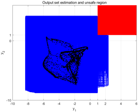
bias vectors are randomly generated. The input set is assumed to be [ x { 0 } ] = [ -5 , 5] × [ -5 , 5] and the unsafe region is ¬S = [1 , ∞ ) × [1 , ∞ ) .
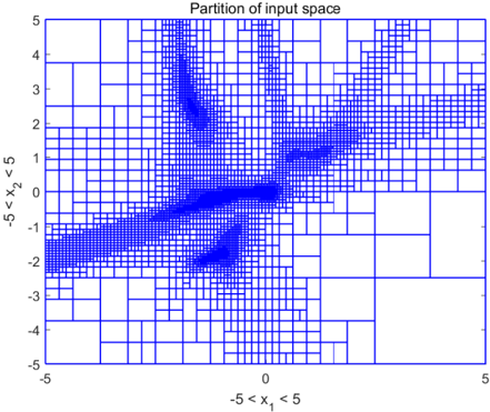
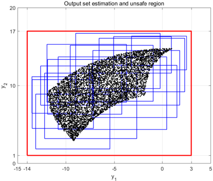
We execute Algorithm 1 with termination parameter ε = 0 . 01 , the safety can be guaranteed by partitioning [ x { 0 } ] into 4095 interval sets. The specification-guided partition of the input space is shown in Figure 1. A non-uniform input space partition is generated based on the specificationguided scheme. An obvious specification-guided effect can be observed in Figure 1. The specification-guided method requires much less computational complexity compared to the approach in [3] which utilizes a uniform partition of input space, and a comparison is listed in Table 1. The computation is carried out using Matlab 2017 on a personal computer with Windows 7, Intel Core i5-4200U, 1.6GHz, 4 GB RAM. It can be seen that the number of interval sets and computational time have been significantly reduced to 3.67% and 7.28%, respectively, compared to those needed in [3]. Figure 2 illustrates the union of 4095 output interval sets, which has no intersection with the unsafe region, illustrating the safety specification is verified. Figure 2 shows that the output interval estimation is guided to be tight when it comes close to unsafe region, and when it is far way from the unsafe area, a coarse estimation is sufficient to verify safety.
Figure 1: Specification-guided bisections of input interval by Algorithm 1. Guided by safety specification, finer partitions are generated when the output intervals are close to the unsafe region, and coarse partitions are generated when the output intervals are far wary.
<details>
<summary>Image 1 Details</summary>
### Visual Description
## 2D Spatial Partition Plot: Partition of input space
### Overview
This image is a 2D plot illustrating a non-uniform, recursive spatial subdivision of a Cartesian coordinate system. The plot consists of a bounding box filled with blue rectangular outlines of varying sizes. The density of these rectangles varies drastically across the plot, indicating an adaptive partitioning algorithm (such as a k-d tree, quadtree, or adaptive mesh refinement) that subdivides the space more finely in specific regions of interest or high complexity, while leaving areas of low complexity as larger, undivided blocks.
### Components/Axes
**Header Region:**
* **Title:** "Partition of input space" (Located at the top-center of the image).
**Main Chart Area:**
* The core visual consists entirely of blue rectangular boxes of varying dimensions. There is no legend, as the data is represented purely by the geometric structure and density of the grid lines.
**X-Axis (Bottom):**
* **Label:** "-5 < x_1 < 5" (Centered below the axis).
* **Scale/Markers:** Linear scale. Visible tick marks and labels are placed at:
* `-5` (Bottom-left corner)
* `0` (Bottom-center)
* `5` (Bottom-right corner)
**Y-Axis (Left):**
* **Label:** "-5 < x_2 < 5" (Rotated 90 degrees counter-clockwise, centered along the left edge).
* **Scale/Markers:** Linear scale. Visible tick marks and labels are placed at integer intervals:
* `5` (Top-left corner)
* `4`, `3`, `2`, `1`
* `0` (Center-left)
* `-1`, `-2`, `-3`, `-4`
* `-5` (Bottom-left corner)
### Detailed Analysis
*Trend Verification Note: Because this is a spatial partition plot rather than a standard line/scatter graph, "trends" are defined by the density gradients of the rectangles (transitioning from large, sparse blocks to small, dense blocks).*
The input space is bounded by $x_1 \in [-5, 5]$ and $x_2 \in [-5, 5]$. The partitioning creates distinct regions of high density (very small rectangles) and low density (large rectangles).
**Low-Density Regions (Sparse / Large Blocks):**
These areas indicate regions where the underlying function or data requires minimal resolution.
* **Bottom-Right:** The largest contiguous blocks are found in the bottom-right quadrant, roughly bounded by $x_1 > 1$ and $x_2 < -1$.
* **Top-Left:** Another sparse region exists in the upper-left, roughly $x_1 < -3$ and $x_2 > 2$.
* **Top-Right:** A sparse region occupies the extreme top-right corner, roughly $x_1 > 3$ and $x_2 > 3$.
**High-Density Regions (Dense / Small Blocks):**
These areas indicate regions of high complexity, steep gradients, or dense data clusters. The dense regions form distinct, interconnected shapes:
1. **Central-Left Band:** A dense band begins at the left edge ($x_1 = -5, x_2 \approx -1.5$) and slopes slightly upward toward the center of the plot ($x_1 \approx 0, x_2 \approx 0$).
2. **Top-Left Plume:** Branching off from the central area, a dense vertical plume extends upwards. It is centered around $x_1 \approx -1.5$ and stretches from $x_2 \approx 1$ up to the top boundary at $x_2 = 5$.
3. **Rightward Band:** From the central hub ($x_1 \approx 0, x_2 \approx 0$), another dense band extends to the right and slightly upwards, passing through $x_1 \approx 2, x_2 \approx 1$ and continuing toward the right edge at $x_1 = 5, x_2 \approx 2$.
4. **Bottom-Center Cluster:** There is a distinct, somewhat isolated dense patch located below the central hub, centered approximately at $x_1 \approx -1, x_2 \approx -2$.
### Key Observations
* The partitioning is highly adaptive; the algorithm clearly targets specific topological features within the space.
* The subdivisions appear to be orthogonal (axis-aligned splits), characteristic of decision trees or k-d trees.
* The dense regions form a roughly star-like or branching manifold with three main arms extending from a central nexus, plus one isolated cluster.
* The transition from sparse to dense is gradual in some areas (e.g., moving from the bottom-right towards the center) and abrupt in others.
### Interpretation
**What the data suggests:**
This image visualizes the "under the hood" mechanics of a mathematical or machine learning model. The grid represents how an algorithm has chosen to divide a 2D space to approximate a function, classify data, or solve an equation. The algorithm uses a recursive splitting method: if a region of space is "simple" (e.g., uniform data class, flat gradient), it leaves it as a large box. If a region is "complex" (e.g., a decision boundary between two classes, a steep curve in a function), it splits the box into smaller pieces to capture the fine details.
**Relationship of elements:**
The relationship between the large and small boxes is one of computational efficiency. By allocating tiny boxes only where necessary (the dark blue bands), the system saves memory and processing power in the empty/simple spaces (the large white boxes).
**Peircean investigative / Reading between the lines:**
The specific shape of the dense regions acts as a "negative space" footprint of an unseen dataset or mathematical function.
* If this is a **Machine Learning Classification** model (like a Decision Tree or Random Forest), the dense blue bands represent the *decision boundaries* separating different classes of data. The algorithm is working very hard to draw precise lines between distinct clusters of data points.
* If this is **Numerical Analysis** (like Adaptive Mesh Refinement for fluid dynamics or heat transfer), the dense bands represent areas of rapid change—such as a shockwave, a thermal front, or a physical boundary within the simulated space.
* The isolated cluster at ($x_1 \approx -1, x_2 \approx -2$) is particularly interesting; it suggests a localized anomaly, a separate cluster of data, or a local minimum/maximum in a function that is disconnected from the main branching structure.
</details>
Figure 2: Output set estimation of neural networks. Blue boxes are output intervals, red area is unsafe region, black dots are 5000 random outputs.
<details>
<summary>Image 2 Details</summary>
### Visual Description
## 2D Plot: Output set estimation and unsafe region
### Overview
This image is a 2D Cartesian plot used in control theory or dynamical systems analysis. It visualizes the relationship between a system's actual trajectory (black), a computed estimation of all possible outputs (blue), and a defined region where the system would fail or be considered unsafe (red). The primary visual narrative is demonstrating that the estimated boundaries of the system's behavior do not intersect with the danger zone.
### Components/Axes
**Header:**
* **Title:** "Output set estimation and unsafe region" (Located at the top center).
**Axes:**
* **X-axis (Horizontal):**
* **Label:** $y_1$ (Located at the bottom center).
* **Scale:** Linear.
* **Tick Marks:** -10, -8, -6, -4, -2, 0, 1, 2, 4, 6.
* *Note:* The inclusion of the '1' tick mark breaks the even-number pattern, specifically to align with the boundary of the red region.
* **Y-axis (Vertical):**
* **Label:** $y_2$ (Rotated 90 degrees, located on the left center).
* **Scale:** Linear.
* **Tick Marks:** -10, 0, 1.
* *Note:* The y-axis is sparsely labeled. The distance between 0 and -10 establishes the scale. The '1' tick mark is explicitly placed just above the '0' to align with the bottom boundary of the red region. The top of the axis extends to approximately +10 based on grid proportions.
**Grid:**
* Light gray grid lines correspond to the major tick marks on both axes.
### Detailed Analysis
The plot contains three distinct data representations, analyzed by spatial positioning and color:
**1. The Unsafe Region (Red Area)**
* **Visual Trend:** A solid, uniform rectangle occupying the top-right quadrant of the plot.
* **Spatial Grounding & Values:**
* The bottom edge aligns perfectly with the $y_2 = 1$ tick mark.
* The left edge aligns perfectly with the $y_1 = 1$ tick mark.
* It extends outward to the right edge ($y_1 = 6$) and the top edge (approx $y_2 = 10$) of the graph area.
* **Mathematical Definition:** The region is defined by the inequalities $y_1 \ge 1$ and $y_2 \ge 1$.
**2. The Output Set Estimation (Blue Area)**
* **Visual Trend:** A large, predominantly solid blue mass occupying the left and central portions of the graph. Upon close inspection of its bottom-right boundary, it is composed of many overlapping, slightly offset rectangles, creating a "staircase" or jagged edge effect.
* **Spatial Grounding & Values:**
* **Left boundary:** Approximately $y_1 = -8.2$.
* **Top boundary:** Approximately $y_2 = 8$.
* **Bottom boundary:** Approximately $y_2 = -9$.
* **Right boundary:** The main vertical edge is at $y_1 = 1$. However, below $y_2 = 1$, the blue area extends further right in a stepped pattern, reaching a maximum of approximately $y_1 = 2.5$ at the bottom right corner (around $y_2 = -8$).
* *Crucial Observation:* The blue area shares a boundary with the red area at $y_1 = 1$ (for $y_2 \ge 1$), but it **does not overlap** the red area.
**3. The Actual Output / Trajectory (Black Pattern)**
* **Visual Trend:** A dense, complex, and seemingly chaotic scatter plot or continuous trajectory line. It features distinct folds, sharp turns, and "wings," resembling a strange attractor from a non-linear dynamical system.
* **Spatial Grounding & Values:**
* It is located entirely within the left-center of the plot.
* **X-bounds:** Spans roughly from $y_1 = -6$ to $y_1 = -0.5$.
* **Y-bounds:** Spans roughly from $y_2 = -7$ to $y_2 = 4$.
* *Crucial Observation:* The black pattern is completely encapsulated by the blue area. It is far away from the red area.
### Key Observations
1. **Encapsulation:** The blue region acts as a strict bounding box (or bounding volume) for the black trajectory. There are no black data points outside the blue area.
2. **Clearance:** There is a distinct visual separation between the actual system behavior (black) and the unsafe region (red).
3. **Algorithmic Artifacts:** The stepped, rectangular nature of the blue region's bottom-right edge strongly suggests it was generated by a computational algorithm that uses interval arithmetic, grid-based reachability, or zonotopes to calculate bounds over time.
### Interpretation
This chart is a visual proof of safety for a dynamical system or control algorithm.
* **The Black Pattern** represents the actual, simulated, or observed states of the system over time. Its complex shape indicates a highly non-linear system.
* **The Red Region** represents a failure state. If the system's output ($y_1, y_2$) enters this zone, the system crashes, breaks, or violates a critical constraint.
* **The Blue Region** represents "Reachability Analysis" or "Output Set Estimation." Because calculating the *exact* future of a complex non-linear system is often computationally impossible, engineers calculate an "over-approximation." The blue area represents *every possible state* the system could theoretically reach, accounting for uncertainties and worst-case scenarios.
**Conclusion drawn from the data:** The system is mathematically proven to be safe. Even though the actual trajectory (black) is complex, the absolute worst-case calculated boundaries (blue) never intersect the failure state (red). The explicit labeling of '1' on both axes serves to highlight the exact mathematical threshold of the unsafe region, proving that the estimation algorithm successfully constrained the system just outside of it.
</details>
## 5.2 Robotic Arm Model
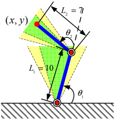
Figure 3: Robotic arm with two joints. The normal working zone of ( θ 1 , θ 2 ) is colored in green θ 1 , θ 2 ∈ [ 5 π 12 , 7 π 12 ] . The buffering zone is in yellow θ 1 , θ 2 ∈ [ π 3 , 5 π 12 ] ∪ [ 7 π 12 , 2 π 3 ] . The forbidden zone is θ 1 , θ 2 ∈ [0 , π 3 ] ∪ [ 2 π 3 , 2 π ] .
<details>
<summary>Image 3 Details</summary>
### Visual Description
## Kinematic Diagram: 2-Link Planar Robotic Arm
### Overview
This image is a technical schematic representing a two-dimensional (planar) robotic manipulator with two revolute joints (an RR linkage). It illustrates the geometric and kinematic parameters required to calculate the position of the end effector, including link lengths, joint angles, and angular constraints (joint limits).
### Components and Variables
The diagram is composed of several distinct visual and textual elements, spatially arranged as follows:
* **Ground/Base:** Located at the bottom, represented by a horizontal black line with diagonal gray hatching beneath it, indicating a fixed, immovable surface.
* **Joints (Nodes):** Three distinct points of articulation/termination:
* **Base Joint:** Bottom-center, resting on the ground line. Depicted as a red circle with a white center and black outline.
* **Elbow Joint:** Center-right. Depicted identically to the base joint.
* **End Effector:** Top-left. Depicted as a solid red circle.
* **Links (Arms):** Two thick blue line segments connecting the joints.
* **Text Labels & Values:**
* **$(x, y)$**: Located at the top-left, adjacent to the end effector.
* **$L_1 = 10$**: Located in the lower-left quadrant, positioned next to a dimension line parallel to the first link.
* **$L_2 = 7$**: Located in the upper-right quadrant, positioned next to a dimension line parallel to the second link.
* **$\theta_1$**: Located at the bottom-right, labeling an angular arc.
* **$\theta_2$**: Located near the center-right (above the elbow joint), labeling an angular arc.
* **Constraint Zones (Shaded Areas):** Cone-shaped sectors originating from the base and elbow joints, featuring a green inner area with a grid pattern and yellow outer edges bounded by dashed lines.
### Content Details
**1. Base and Link 1 ($L_1$)**
* **Positioning:** Originates at the Base Joint on the ground. The thick blue line extends upwards and slightly to the right.
* **Length:** A dimension line with arrows at both ends runs parallel to this link. The text explicitly states **$L_1 = 10$**.
* **Angle ($\theta_1$):** An arc with an arrowhead originates from the right-side horizontal ground line and curves counter-clockwise to meet Link 1. This denotes the absolute base angle, labeled **$\theta_1$**. Visually, this angle is approximately $75^\circ$ to $80^\circ$.
* **Constraints:** A shaded sector originates from the base joint. The central portion of the sector is green with a grid, flanked by solid yellow regions. Dashed lines mark the absolute outer boundaries of the yellow regions. This visually represents the allowable range of motion for $\theta_1$.
**2. Elbow and Link 2 ($L_2$)**
* **Positioning:** Originates at the Elbow Joint (connecting $L_1$ and $L_2$). The thick blue line extends upwards and to the left.
* **Reference Line:** A dashed black line extends straight out from the Elbow Joint, continuing the exact trajectory/vector of Link 1.
* **Length:** A dimension line with arrows at both ends runs parallel to this second link. The text explicitly states **$L_2 = 7$**.
* **Angle ($\theta_2$):** An arc with an arrowhead originates from the dashed reference line and curves counter-clockwise to meet Link 2. This denotes the relative joint angle, labeled **$\theta_2$**. Visually, this angle is obtuse, approximately $135^\circ$ to $150^\circ$.
* **Constraints:** Similar to Link 1, a shaded sector (green grid center, yellow edges, dashed boundaries) originates from the Elbow Joint, representing the allowable range of motion for $\theta_2$ relative to Link 1.
**3. End Effector**
* **Positioning:** The terminal end of Link 2.
* **Coordinates:** Labeled explicitly as **$(x, y)$**, representing the Cartesian coordinates of the robot's tip in 2D space.
### Key Observations
* **Relative vs. Absolute Angles:** The diagram clearly distinguishes between an absolute angle ($\theta_1$ is measured from the fixed ground) and a relative angle ($\theta_2$ is measured from the extended axis of the previous link). This is standard Denavit-Hartenberg convention for robotic kinematics.
* **Visualizing Limits:** The green and yellow shaded regions are critical. They do not represent physical objects, but rather the mathematical/mechanical limits of the joints. The green area likely represents the normal/safe operating range, while the yellow areas represent warning zones approaching the mechanical hard-stops (dashed lines).
* **Proportions:** The visual lengths of the blue lines roughly correspond to their stated values ($L_1=10$ is visibly longer than $L_2=7$).
### Interpretation
This diagram is a classic representation of a **Forward Kinematics** problem in robotics. Forward kinematics involves calculating the position of the end effector $(x, y)$ given the link lengths ($L_1, L_2$) and the joint angles ($\theta_1, \theta_2$).
Based on the geometric relationships explicitly detailed in the image, the mathematical equations governing this system are implied:
* $x = L_1 \cos(\theta_1) + L_2 \cos(\theta_1 + \theta_2)$
* $y = L_1 \sin(\theta_1) + L_2 \sin(\theta_1 + \theta_2)$
**Reading between the lines (Peircean investigative):**
The inclusion of the green and yellow constraint zones elevates this from a simple geometry problem to a practical robotics engineering diagram. In real-world applications, joints cannot rotate infinitely due to internal wiring, motors, or physical casing.
* If an engineer were writing a path-planning algorithm for this arm, they would use the dashed lines as absolute constraints (e.g., $\theta_{1_{min}} \le \theta_1 \le \theta_{1_{max}}$).
* The transition from green to yellow suggests a control system where moving into the yellow zone might trigger a software speed reduction to prevent mechanical damage upon hitting the dashed-line limit.
* Furthermore, knowing these limits is essential for **Inverse Kinematics** (calculating required angles to reach a specific $(x,y)$ point), as some points in space might be mathematically reachable but physically impossible due to the joint limits shown by the shaded cones.
</details>
In [3], a learning forward kinematics of a robotic arm model with two joints is proposed, shown in Figure 3. The learning task is using a feedforward neural network to predict the position ( x, y ) of the end with knowing the joint angles ( θ 1 , θ 2 ) . The input space [0 , 2 π ] × [0 , 2 π ] for ( θ 1 , θ 2 ) is classified into three zones for its operations: normal working zone θ 1 , θ 2 ∈ [ 5 π 12 , 7 π 12 ] , buffering zone θ 1 , θ 2 ∈ [ π 3 , 5 π 12 ] ∪ [ 7 π 12 , 2 π 3 ] and forbidden zone θ 1 , θ 2 ∈ [0 , π 3 ] ∪ [ 2 π 3 , 2 π ] . The detailed formulation for this robotic arm model and neural network training can be found in [3].
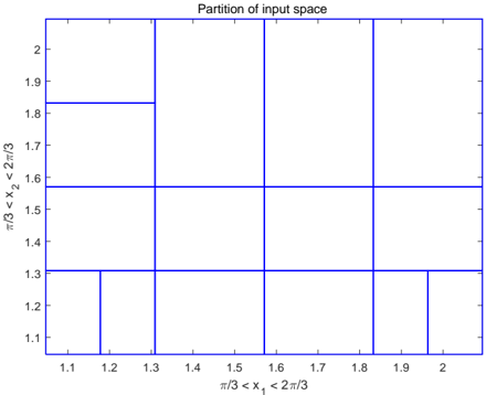
The safety specification for the position ( x, y ) is S = { ( x, y ) | -14 ≤ x ≤ 3 and 1 ≤ y ≤ 17 } . The input set of the robotic arm is the union of normal working and buffering zones, that is ( θ 1 , θ 2 ) ∈ [ π 3 , 2 π 3 ] × [ π 3 , 2 π 3 ] . In the safety point of view, the neural network needs to be verified that all the outputs produced by the inputs in the normal working
zone and buffering zone will satisfy safety specification S . In [3], a uniform partition for input space is used, and thus 729 intervals are produced to verify the safety property. Using our specification-guided approach, the safety can be guaranteed by partitioning the input space into only 15 intervals, see Figure 4 and Figure 5. Due to the small number of intervals involved in the verification process, the computational time is only 0.27 seconds for specification-guided approach.
Figure 4: 15 sub-intervals for robotic arm safety verification.
<details>
<summary>Image 4 Details</summary>
### Visual Description
## 2D Plot: Partition of Input Space
### Overview
The image displays a 2D Cartesian coordinate plot showing a rectangular area that has been subdivided into smaller, non-uniform rectangular regions. The plot represents a mathematical or computational "partition of input space," where a continuous 2D domain is discretized into specific bounding boxes. The grid lines are solid blue, set against a white background.
### Components/Axes
**1. Header (Top Center)**
* **Title:** "Partition of input space"
**2. X-Axis (Bottom)**
* **Label:** $\pi/3 < x_1 < 2\pi/3$ (Centered below the axis).
* **Scale/Range:** The visual axis begins slightly before 1.1 and ends slightly after 2.0, corresponding to the mathematical range of approximately $[1.047, 2.094]$.
* **Tick Markers:** 1.1, 1.2, 1.3, 1.4, 1.5, 1.6, 1.7, 1.8, 1.9, 2 (Spaced evenly at 0.1 intervals).
**3. Y-Axis (Left)**
* **Label:** $\pi/3 < x_2 < 2\pi/3$ (Rotated 90 degrees counter-clockwise, centered left of the axis).
* **Scale/Range:** Identical to the X-axis, representing approximately $[1.047, 2.094]$.
* **Tick Markers:** 1.1, 1.2, 1.3, 1.4, 1.5, 1.6, 1.7, 1.8, 1.9, 2 (Spaced evenly at 0.1 intervals).
### Detailed Analysis
The main chart area consists of a bounding box defined by the limits $\pi/3$ and $2\pi/3$ on both axes. This space is divided by a series of orthogonal blue lines. Based on the axis labels and visual placement, these lines correspond to recursive bisections (midpoints) of the mathematical intervals.
**Primary Grid Lines (Spanning the entire width/height):**
* **Vertical Lines ($x_1$):**
* $x_1 \approx 1.31$ (Mathematically deduced as $5\pi/12$, the midpoint of $[\pi/3, \pi/2]$)
* $x_1 \approx 1.57$ (Mathematically deduced as $\pi/2$, the midpoint of $[\pi/3, 2\pi/3]$)
* $x_1 \approx 1.83$ (Mathematically deduced as $7\pi/12$, the midpoint of $[\pi/2, 2\pi/3]$)
* **Horizontal Lines ($x_2$):**
* $x_2 \approx 1.31$ (Mathematically deduced as $5\pi/12$)
* $x_2 \approx 1.57$ (Mathematically deduced as $\pi/2$)
**Secondary/Minor Grid Lines (Partial spans):**
* **Top-Left Region:** A horizontal line at $x_2 \approx 1.83$ ($7\pi/12$) splits the column where $x_1 < 1.31$ and $x_2 > 1.57$.
* **Bottom-Left Region:** A vertical line at $x_1 \approx 1.18$ (Mathematically deduced as $3\pi/8$, the midpoint of $[\pi/3, 5\pi/12]$) splits the box where $x_1 < 1.31$ and $x_2 < 1.31$.
* **Bottom-Right Region:** A vertical line at $x_1 \approx 1.96$ (Mathematically deduced as $5\pi/8$, the midpoint of $[7\pi/12, 2\pi/3]$) splits the box where $x_1 > 1.83$ and $x_2 < 1.31$.
**Resulting Partitions:**
The space is divided into 15 distinct rectangular regions of varying sizes. The largest regions are located in the upper-right quadrant, while the smallest, most densely partitioned regions are located in the bottom-left, bottom-right, and top-left extremities.
### Key Observations
* **Non-Uniformity:** The grid is not a standard, equally spaced mesh. It exhibits localized refinement.
* **Recursive Bisection Pattern:** The placement of the lines strongly suggests a binary space partitioning algorithm. The domain is split in half ($\pi/2$), then those halves are split ($5\pi/12$, $7\pi/12$), and specific sub-regions are split again ($3\pi/8$, $5\pi/8$).
* **Asymmetry:** While the primary vertical lines divide the space into four columns, the horizontal lines only divide it into three main rows, with further subdivision only occurring in specific localized boxes.
### Interpretation
This image demonstrates a **spatially adaptive partitioning strategy**, commonly used in computational mathematics, machine learning, and numerical analysis.
* **Underlying Function Behavior:** In techniques like Adaptive Mesh Refinement (AMR) for solving partial differential equations, or in decision tree algorithms (like k-d trees or CART), a space is subdivided more finely in areas where the underlying data or function is complex, highly variable, or contains steep gradients. Conversely, areas with large, undivided rectangles (like the center and top-right) suggest that the underlying function is relatively smooth, uniform, or of less interest in those regions.
* **Algorithmic Logic:** The strict adherence to midpoints (bisections of intervals based on fractions of $\pi$) indicates a programmatic, recursive algorithm rather than arbitrary manual drawing. The algorithm evaluates a region, determines if an error threshold or variance limit is exceeded, and if so, splits the region in half along one or both axes.
* **Focus Areas:** The higher density of partitions along the bottom edge ($x_2 < 1.31$) and the top-left corner indicates that the system required higher resolution or encountered more complexity in these specific boundary areas of the input space.
</details>
## 5.3 Handwriting Image Recognition
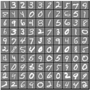
In this handwriting image recognition task, we use 5000 training examples of handwritten digits which is a subset of the MNIST handwritten digit dataset (http://yann.lecun.com/exdb/mnist/), examples from the dataset are shown in Figure 6. Each training example is a 20 pixel by 20 pixel grayscale image of the digit. Each pixel is represented by a floating point number indicating the grayscale intensity at that location. We first train a neural network with 400 inputs, one hidden layer with 25 neurons and 10 output units corresponding to the 10 digits. The activation functions for both hidden and output layers are sigmoid functions. A trained neural network with about 97.5% accuracy is obtained.
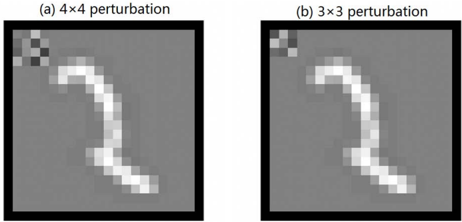
Under adversarial perturbations, the neural network may produce a wrong prediction. For example in Figure 7(a) which is an image of digit 2 , the label predicted by the neural network will turn to 1 as a 4 × 4 perturbation belonging to [ -0 . 5 , 0 . 5] attacks the left-top corner of the image. With our developed verification method, we wish to prove that the neural network is robust to certain classes of perturbations, that is no perturbation belonging to those classes can alter the prediction of the neural network for a perturbed image. Since there exists one adversarial example for 4 perturbations at the left-top corner, it implies this image is not robust to this class of perturbation. We consider another class of perturbations, 3 × 3 perturbations at the left-top corner, see Figure 7(b). Us-
Figure 5: Safety verification for neural network of robotic arm. Blue boxes are output intervals, red box are boundary for unsafe region, black dots are 5000 random outputs. 15 output intervals are sufficient to prove the safety.
<details>
<summary>Image 5 Details</summary>
### Visual Description
## 2D Scatter Plot with Bounding Boxes: Output Set Estimation and Unsafe Region
### Overview
The image is a 2D Cartesian plot displaying a dense scatter plot of data points overlaid with multiple overlapping rectangular bounding boxes, all enclosed within a single, larger rectangular boundary. The chart visualizes a mathematical or computational concept, likely related to reachability analysis, formal verification, or control theory, where a complex set of outputs is approximated by simpler geometric shapes to check against defined constraints.
### Components/Axes
**Header:**
* **Title:** "Output set estimation and unsafe region" (Located top-center).
**Axes:**
* **X-axis (Bottom):** Labeled as "$y_1$". It features a linear scale with major grid lines.
* *Markers:* -15, -14, -10, -5, 0, 3, 5.
* *Note:* The markers -14 and 3 are specifically placed to align with the vertical edges of the red rectangle, rather than following the standard intervals of 5.
* **Y-axis (Left):** Labeled as "$y_2$" (rotated 90 degrees counter-clockwise). It features a linear scale with major grid lines.
* *Markers:* 0, 1, 10, 17, 20.
* *Note:* The markers 1 and 17 are specifically placed to align with the horizontal edges of the red rectangle, deviating from the standard intervals of 10.
**Legend/Color Coding (Inferred from Title and Context):**
* *Note: There is no explicit legend box. The following is deduced from the title and visual hierarchy.*
* **Black Dots:** Represent the actual "Output set" (likely generated via Monte Carlo simulation or empirical sampling).
* **Blue Rectangles:** Represent the "Output set estimation" (an over-approximation of the black dots using a union of intervals/boxes).
* **Red Rectangle:** Represents the boundary related to the "unsafe region" mentioned in the title.
### Detailed Analysis
**1. The Red Boundary (Unsafe Region / Constraint):**
* *Visual Trend:* A single, thick red line forming a perfect rectangle.
* *Spatial Grounding:* It dominates the chart area, acting as an outer envelope for all other data.
* *Data Points:* Based on the specific axis markers, the red rectangle is defined exactly by the coordinates:
* $y_1$ (X-axis) bounds: $[-14, 3]$
* $y_2$ (Y-axis) bounds: $[1, 17]$
**2. The Black Scatter Plot (Actual Output Set):**
* *Visual Trend:* Thousands of dense black dots forming a cohesive, asymmetrical, roughly fan-like or crescent shape. The left side is wider and somewhat flat, while it tapers to a narrower point on the right side. The bottom edge is convex, and the top edge is slightly concave.
* *Spatial Grounding:* Centered within the plot, entirely contained within the red rectangle.
* *Approximate Bounds:*
* Leftmost point: $\approx -13$ on $y_1$
* Rightmost point: $\approx 1.5$ on $y_1$
* Lowest point: $\approx 2$ on $y_2$
* Highest point: $\approx 15$ on $y_2$
**3. The Blue Rectangles (Output Set Estimation):**
* *Visual Trend:* Approximately 15 to 20 overlapping blue rectangles of varying widths and heights.
* *Spatial Grounding:* They are clustered around the black scatter plot. Every blue rectangle contains a portion of the black dots. Collectively, the union of all blue rectangles completely covers (over-approximates) the entire black scatter plot.
* *Relationship to Red Box:* All blue rectangles are strictly contained within the boundaries of the red rectangle. The leftmost blue box approaches $y_1 \approx -13.5$, the rightmost approaches $y_1 \approx 2.5$, the lowest approaches $y_2 \approx 1.5$, and the highest approaches $y_2 \approx 16.5$. None cross the $-14, 3, 1,$ or $17$ thresholds.
### Key Observations
* **Strict Containment:** The most critical visual takeaway is the hierarchy of containment: The actual data (black dots) is entirely inside the estimation (blue boxes), and the estimation (blue boxes) is entirely inside the defined boundary (red box).
* **Conservative Estimation:** The blue boxes cover areas where there are no black dots (empty white space within the blue lines). This indicates a "conservative" or "over-approximated" estimation method.
* **Custom Axis Labeling:** The creator of the chart intentionally added non-standard tick marks (-14, 3 on X; 1, 17 on Y) specifically to provide exact numerical values for the red boundary box, highlighting its importance.
### Interpretation
**Contextual Meaning (Peircean Deduction):**
This image is a classic visualization from the field of **formal verification of dynamical systems or neural networks** (specifically, reachability analysis).
* **The Black Dots** represent the true reachable set of a system's outputs given a set of inputs. Because calculating the exact non-linear boundaries of this set is computationally impossible, it is approximated.
* **The Blue Boxes** represent the mathematical algorithm's attempt to bound this complex shape using simpler geometry (likely interval arithmetic or zonotopes). The algorithm guarantees that the true outputs (black) will *always* be inside the estimation (blue).
* **The Red Box** represents a critical system constraint. The title mentions "unsafe region." In verification, you typically want to prove that your system *never* enters an unsafe region.
* *Nuance:* If the red box itself is the "unsafe region," then this system is failing catastrophically, as all outputs are inside it.
* *More Likely Scenario:* The red box represents the **Safe Set**, and anything *outside* the red box is the "unsafe region." Therefore, the goal of the chart is to prove safety. Because the over-approximated estimation (blue boxes) never crosses the red line, the engineers can mathematically guarantee that the actual system (black dots) will never enter the unsafe region (outside the red box).
**Conclusion:**
The data demonstrates a successful safety verification. The estimation algorithm successfully bounded the complex output set, and this bounding geometry remained strictly within the defined safety tolerances ($y_1 \in [-14, 3]$, $y_2 \in [1, 17]$), proving the system avoids the unsafe region.
</details>
Figure 6: Examples from the MNIST handwritten digit dataset.
<details>
<summary>Image 6 Details</summary>
### Visual Description
## Image Grid: Handwritten Digits Sample (MNIST Dataset Style)
### Overview
The image displays a 10x10 grid containing 100 individual grayscale images of handwritten Arabic numerals (0 through 9). The digits are rendered in white/light gray against a uniform dark gray background. The image is highly characteristic of a sample batch from the MNIST (Modified National Institute of Standards and Technology) database, which is a standard benchmark dataset used in machine learning and computer vision for training image processing systems.
### Components/Axes
* **Axes/Scales:** There are no X or Y axes, scales, or tick marks present.
* **Legends/Labels:** There are no textual labels, titles, or legends.
* **Grid Structure:** The image is divided by thin black lines into a 10-row by 10-column matrix, yielding 100 distinct cells. Each cell acts as a bounding box for a single digit.
### Content Details
Below is the precise transcription of the handwritten digits, mapped spatially to their exact row and column positions within the grid.
*Note: Due to the nature of human handwriting, a few digits exhibit structural ambiguity (e.g., Row 7, Column 1 resembles a '4' with an extra vertical stroke; Row 1, Column 5 is a '3' with artifact dots). The transcription represents the most highly probable intended digit.*
| Row \ Col | C1 | C2 | C3 | C4 | C5 | C6 | C7 | C8 | C9 | C10 |
| :--- | :--- | :--- | :--- | :--- | :--- | :--- | :--- | :--- | :--- | :--- |
| **R1** | 1 | 3 | 2 | 3 | 3 | 2 | 2 | 5 | 7 | 9 |
| **R2** | 8 | 4 | 4 | 0 | 0 | 1 | 2 | 6 | 5 | 1 |
| **R3** | 6 | 9 | 6 | 4 | 8 | 1 | 5 | 6 | 3 | 8 |
| **R4** | 6 | 3 | 3 | 3 | 2 | 7 | 3 | 0 | 1 | 0 |
| **R5** | 9 | 7 | 4 | 7 | 3 | 8 | 9 | 4 | 6 | 2 |
| **R6** | 2 | 8 | 5 | 4 | 0 | 0 | 1 | 0 | 8 | 5 |
| **R7** | 4 | 4 | 5 | 6 | 9 | 0 | 5 | 9 | 0 | 0 |
| **R8** | 5 | 0 | 9 | 3 | 5 | 7 | 5 | 9 | 0 | 0 |
| **R9** | 2 | 4 | 5 | 0 | 0 | 6 | 0 | 2 | 9 | 9 |
| **R10** | 2 | 2 | 6 | 9 | 0 | 2 | 6 | 4 | 4 | 2 |
### Key Observations
* **High Variance in Stroke:** There is significant variation in stroke thickness, slant, and overall morphology for the same digits.
* *Example:* The '1's range from perfectly vertical lines (R1, C1) to heavily slanted lines (R2, C10).
* *Example:* The '2's feature both looped bases (R1, C3) and sharp, angled bases (R10, C1).
* *Example:* The '7's include both standard strokes (R1, C9) and crossed strokes (R5, C2).
* **Artifacts/Noise:** Row 1, Column 5 contains a '3' with three distinct white dots (noise) to the right of the digit within its cell.
* **Distribution:** The digits appear to be randomly shuffled rather than ordered sequentially or grouped by class.
* **Centering:** All digits appear to be roughly size-normalized and centered within their respective grid cells.
### Interpretation
* **Purpose of the Data:** This image does not represent a chart of quantitative trends; rather, it is a visualization of raw data used for Optical Character Recognition (OCR). It demonstrates the input layer for a machine learning model (likely a Convolutional Neural Network).
* **The Challenge of Generalization:** The primary takeaway from this visual data is the inherent complexity of human handwriting. A successful algorithm must learn the underlying topological features of a "3" or a "5" while ignoring the vast superficial differences in slant, thickness, and minor artifacts (like the dots in R1, C5).
* **Preprocessing Indicators:** The uniform gray background (rather than pure black) suggests that the image data may have undergone preprocessing, such as mean subtraction or normalization, which is a common step before feeding image matrices into neural networks to stabilize the learning process. The strict bounding boxes confirm the data has been segmented and scaled to a uniform pixel dimension (traditionally 28x28 pixels per cell for MNIST).
</details>
ing Algorithm 1, the neural network can be proved to be robust to all 3 × 3 perturbations located at at the left-top corner of the image, after 512 bisections.
Moreover, applying Algorithm 1 to all 5000 images with 3 × 3 perturbations belonging to [ -0 . 5 , 0 . 5] and located at the left-top corner, it can be verified that the neural network is robust to this class of perturbations for all images. This result means this class of perturbations will not affect the prediction accuracy of the neural network. The neural network is able to maintain its 97.5% accuracy even subject to any perturbations belonging to this class of 3 × 3 perturbations.
Figure 7: Perturbed image of digit 2 with perturbation in [ -0 . 5 . 0 . 5] . (a) 4 × 4 perturbation at the left-top corner, the neural network will wrongly label it as digit 1. (b) 3 × 3 perturbation at the left-top corner, the neural network can be proved to be robust for this class of perturbations.
<details>
<summary>Image 7 Details</summary>
### Visual Description
## Image Comparison: Localized Adversarial Perturbations
### Overview
The image presents a side-by-side comparison of two grayscale digital images. Both images feature the identical central subject: a pixelated, handwritten digit (resembling a '2') on a uniform gray background, framed by a thick black border. The primary focus of the image is the introduction of localized, square patches of visual noise (perturbations) located in the top-left corners of the gray canvas.
### Components and Layout
* **Left Panel Header:** Text reading "(a) 4×4 perturbation" centered above the left image.
* **Right Panel Header:** Text reading "(b) 3×3 perturbation" centered above the right image.
* **Main Subject (Both Panels):** A white/light-gray curved stroke forming a handwritten numeral '2', positioned centrally.
* **Background (Both Panels):** A flat, medium-gray tone.
* **Frame (Both Panels):** A thick, solid black border enclosing the gray background and the digit.
* **Variable Component:** A small, square grid of altered pixels in the top-left corner, immediately inside the black border.
### Content Details
**Panel (a) - Left Image:**
* **Label:** (a) 4×4 perturbation
* **Perturbation Location:** Top-left corner of the gray background.
* **Perturbation Characteristics:** A distinct 4 by 4 grid of pixels (16 pixels total). The pixels within this grid exhibit varying intensities, including dark gray, light gray, and near-white, creating a randomized, checkerboard-like noise pattern.
* **Subject Interaction:** The perturbation is spatially isolated from the handwritten digit. There is a clear gap of unaltered gray background between the noise patch and the top of the numeral.
**Panel (b) - Right Image:**
* **Label:** (b) 3×3 perturbation
* **Perturbation Location:** Top-left corner of the gray background, in the exact same anchor position as panel (a).
* **Perturbation Characteristics:** A distinct 3 by 3 grid of pixels (9 pixels total). Similar to panel (a), it contains varying intensities of grayscale pixels. It occupies a smaller physical area than the perturbation in panel (a).
* **Subject Interaction:** Identical to panel (a), the perturbation is spatially isolated from the handwritten digit.
### Key Observations
* **Subject Constancy:** The central handwritten digit and the black border are pixel-perfect matches across both images. The *only* variable is the noise patch in the top-left corner.
* **Spatial Isolation:** The noise patches do not obscure, overlap, or touch the primary subject (the digit).
* **Dimensionality:** The text explicitly defines the dimensions of the noise patches (4x4 pixels vs. 3x3 pixels), which is visually confirmed by the grid sizes in the respective corners.
### Interpretation
* **Context:** This image is a classic visualization from a technical paper in the field of **Adversarial Machine Learning**, specifically focusing on Computer Vision. The handwritten digit is highly characteristic of the MNIST dataset, a standard benchmark in machine learning.
* **What the Data Demonstrates:** The image illustrates a "patch attack" or "localized adversarial perturbation." In machine learning, an attacker alters a small number of pixels to intentionally cause a neural network (like a Convolutional Neural Network) to misclassify the image. To a human, the image is obviously still a '2'. To a compromised AI, the specific pattern of noise in the corner forces a wrong prediction (e.g., classifying it as a '7' or '0').
* **Significance of the Comparison (4x4 vs 3x3):** The authors are comparing the size of the adversarial patch.
* A **4x4 patch** (16 pixels) gives the attacker more "degrees of freedom" (more variables to optimize) to successfully fool the AI, but alters more of the original image.
* A **3x3 patch** (9 pixels) is a more constrained, stealthier attack. It alters fewer pixels (a lower $L_0$ norm), making it harder to detect visually or programmatically, but it may be mathematically harder to find a 3x3 pattern that successfully breaks the model compared to a 4x4 pattern.
* **Peircean Investigative Deduction (Reading between the lines):** Because the perturbation is placed in the corner—completely detached from the digit itself—this graphic highlights a specific vulnerability in how the AI processes images. It proves that the AI model is not just looking at the shape of the digit; it is highly sensitive to background/contextual pixels. The model has learned spurious correlations in the background space, allowing an attacker to hijack the classification without ever touching the actual subject of the image.
</details>
## 6 Conclusion and Future Work
In this paper, we introduce a specification-guided approach for safety verification of feedforward neural networks with general activation functions. By formulating the safety verification problem into the framework of interval analysis, a fast computation formula for calculating output intervals of feedforward neural networks is developed. Then, a safety verification algorithm which is called specification-guided is developed. The algorithm is specification-guided since the activation of bisection actions are totally determined by the existence of intersections between the computed output intervals and unsafe sets. This distinguishing feature makes the specification-guided approach be able to avoid unnecessary computations and significantly reduce the computational cost. Several experiments are proposed to show the advantages of our approach.
Though our approach is general in the sense that it is not tailored to specific activation functions, the specification-guided idea has potential to be further applied to other methods dealing with specific activation functions such as ReLU neural networks to enhance their scalability. Moreover, since our approach can compute the output intervals of a neural network, it can be incorporated with other reachable set estimation methods to compute the dynamical system models with neural network components inside such as extension of [3] to closed-loop systems [19] and neural network models of nonlinear dynamics [20].
## References
- [1] C. Szegedy, W. Zaremba, I. Sutskever, J. Bruna, D. Erhan, I. Goodfellow, and R. Fergus, 'Intriguing properties of neural networks,' in International Conference on Learning Representations , 2014.
- [2] G. Katz, C. Barrett, D. Dill, K. Julian, and M. Kochenderfer, 'Reluplex: An efficient SMT solver for verify-
3. ing deep neural networks,' in International Conference on Computer Aided Verification , pp. 97-117, Springer, 2017.
- [3] W. Xiang, H.-D. Tran, and T. T. Johnson, 'Output reachable set estimation and verification for multi-layer neural networks,' IEEE Transactions on Neural Network and Learning Systems , vol. 29, no. 11, pp. 5777-5783, 2018.
- [4] E. Clarke, O. Grumberg, S. Jha, Y. Lu, and H. Veith, 'Counterexample-guided abstraction refinement,' in International Conference on Computer Aided Verification , pp. 154-169, Springer, 2000.
- [5] N. Een, A. Mishchenko, and R. Brayton, 'Efficient implementation of property directed reachability,' in Proceedings of the International Conference on Formal Methods in Computer-Aided Design , pp. 125-134, FMCAD Inc, 2011.
- [6] S. Skelboe, 'Computation of rational interval functions,' BIT Numerical Mathematics , vol. 14, no. 1, pp. 87-95, 1974.
- [7] W. Xiang, H.-D. Tran, and T. T. Johnson, 'Reachable set computation and safety verification for neural networks with ReLU activations,' arXiv preprint arXiv: 1712.08163 , 2017.
- [8] T. Gehr, M. Mirman, D. Drachsler-Cohen, P. Tsankov, S. Chaudhuri, and M. Vechev, ' AI 2 : Safety and robustness certification of neural networks with abstract interpretation,' in Security and Privacy (SP), 2018 IEEE Symposium on , 2018.
- [9] R. Ehlers, 'Formal verification of piecewise linear feedforward neural networks,' in International Symposium on Automated Technology for Verification and Analysis , pp. 269-286, Springer, 2017.
- [10] A. Lomuscio and L. Maganti, 'An approach to reachability analysis for feed-forward ReLU neural networks,' arXiv preprint arXiv:1706.07351 , 2017.
- [11] S. Dutta, S. Jha, S. Sanakaranarayanan, and A. Tiwari, 'Output range analysis for deep neural networks,' arXiv preprint arXiv:1709.09130 , 2017.
- [12] S. Dutta, S. Jha, S. Sankaranarayanan, and A. Tiwari, 'Output range analysis for deep feedforward neural networks,' in NASA Formal Methods Symposium , pp. 121138, Springer, 2018.
- [13] L. Pulina and A. Tacchella, 'An abstraction-refinement approach to verification of artificial neural networks,' in International Conference on Computer Aided Verification , pp. 243-257, Springer, 2010.
- [14] L. Pulina and A. Tacchella, 'Challenging SMT solvers to verify neural networks,' AI Communications , vol. 25, no. 2, pp. 117-135, 2012.
- [15] M. Fr¨ anzle and C. Herde, 'HySAT: An efficient proof engine for bounded model checking of hybrid systems,' Formal Methods in System Design , vol. 30, no. 3, pp. 179-198, 2007.
- [16] X. Huang, M. Kwiatkowska, S. Wang, and M. Wu, 'Safety verification of deep neural networks,' in International Conference on Computer Aided Verification , pp. 3-29, Springer, 2017.
- [17] W. Ruan, X. Huang, and M. Kwiatkowska, 'Reachability analysis of deep neural networks with provable guarantees,' arXiv preprint arXiv:1805.02242 , 2018.
- [18] R. E. Moore, R. B. Kearfott, and M. J. Cloud, Introduction to interval analysis , vol. 110. Siam, 2009.
- [19] W. Xiang, D. M. Lopez, P. Musau, and T. T. Johnson, 'Reachable set estimation and verification for neural network models of nonlinear dynamic systems,' in Safe, Autonomous and Intelligent Vehicles , pp. 123-144, Springer, 2019.
- [20] W. Xiang, H. Tran, J. A. Rosenfeld, and T. T. Johnson, 'Reachable set estimation and safety verification for piecewise linear systems with neural network controllers,' in 2018 Annual American Control Conference (ACC) , pp. 1574-1579, June 2018.