# Binaural LCMV Beamforming with Partial Noise Estimation
**Authors**: Nico Gößling, Elior Hadad, Sharon Gannot, Simon Doclo
## Binaural LCMV Beamforming with Partial Noise Estimation
Nico G¨ oßling, Student Member, IEEE, Elior Hadad, Member, IEEE, Sharon Gannot, Senior Member, IEEE and Simon Doclo, Senior Member, IEEE
Abstract -Besides reducing undesired sources, i.e., interfering sources and background noise, another important objective of a binaural beamforming algorithm is to preserve the spatial impression of the acoustic scene, which can be achieved by preserving the binaural cues of all sound sources. While the binaural minimum variance distortionless response (BMVDR) beamformer provides a good noise reduction performance and preserves the binaural cues of the desired source, it does not allow to control the reduction of the interfering sources and distorts the binaural cues of the interfering sources and the background noise. Hence, several extensions have been proposed. First, the binaural linearly constrained minimum variance (BLCMV) beamformer uses additional constraints, enabling to control the reduction of the interfering sources while preserving their binaural cues. Second, the BMVDR with partial noise estimation (BMVDR-N) mixes the output signals of the BMVDR with the noisy reference microphone signals, enabling to control the binaural cues of the background noise. Aiming at merging the advantages of both extensions, in this paper we propose the BLCMV with partial noise estimation (BLCMV-N). We show that the output signals of the BLCMV-N can be interpreted as a mixture between the noisy reference microphone signals and the output signals of a BLCMV using an adjusted interference scaling parameter. We provide a theoretical comparison between the BMVDR, the BLCMV, the BMVDR-N and the proposed BLCMV-N in terms of noise and interference reduction performance and binaural cue preservation. Experimental results using recorded signals as well as the results of a perceptual listening test show that the BLCMV-N is able to preserve the binaural cues of an interfering source (like the BLCMV), while enabling to trade off between noise reduction performance and binaural cue preservation of the background noise (like the BMVDR-N).
Index Terms -Binaural cues, binaural noise reduction, MVDR beamformer, LCMV beamformer, hearing devices
## I. INTRODUCTION
B EAMFORMING algorithms for head-mounted assistive hearing devices (e.g., hearing aids, earbuds and hearables) are crucial to improve speech quality and speech intelligibility in noisy acoustic environments. Assuming a binaural configuration where both devices exchange their microphone signals, the information captured by all microphones on both
This work was funded by the Deutsche Forschungsgemeinschaft (DFG, German Research Foundation) - Project ID 352015383 (SFB 1330 B2) and Project ID 390895286 (EXC 2177/1) and the Israeli Ministry of Science and Technology, #88962, 2019.
E. Hadad and S. Gannot are with the Faculty of Engineering, BarIlan University, Ramat-Gan, 5290002, Israel (e-mail: elior.hadad@biu.ac.il; sharon.gannot@biu.ac.il).
N. G¨ oßling and S. Doclo are with the Department of Medical Physics and Acoustics and the Cluster of Excellence Hearing4all, University of Oldenburg, 26111 Oldenburg, Germany (e-mail: nico.goessling@uol.de; simon.doclo@uol.de).
sides of the head can be exploited [1]-[3]. Besides reducing interfering sources (e.g., competing speakers) and background noise (e.g., diffuse babble noise), another important objective of a binaural beamforming algorithm is the preservation of the listener's spatial impression of the acoustic scene. This can be achieved by preserving the binaural cues of all sound sources, i.e., the interaural level difference (ILD) and the interaural time difference (ITD) for coherent sources (desired source and interfering sources) and the interaural coherence (IC) for incoherent sound fields (background noise) [4]. Binaural cues play a major role for spatial perception, i.e., to localize sound sources and to determine the spatial width or diffuseness of a sound field [5], and are very important for speech intelligibility due to so-called binaural unmasking [6], [7].
Unlike monaural beamforming algorithms, binaural beamforming algorithms need to generate two output signals (i.e., one for each ear), hence typically processing all available microphone signals from both devices by two different spatial filters [8]-[19]. A frequently used binaural beamforming algorithm is the binaural minimum variance distortionless response (BMVDR) beamformer, which aims at minimizing the power spectral density (PSD) of the noise component in the output signals while preserving the desired source component in the reference microphone signals on the left and the right device [2], [3], [11]. While the BMVDR provides a good noise reduction performance and preserves the binaural cues of the desired source, it does not allow to control the reduction of the interfering sources and distorts the binaural cues of the undesired sources (interfering sources and background noise). More specifically, after applying the BMVDR the binaural cues of the undesired sources are equal to the binaural cues of the desired source, such that all sources are perceived as coming from the same direction, which is obviously undesired. Hence, several extensions of the BMVDR have been proposed. On the one hand, the binaural linearly constrained minimum variance (BLCMV) beamformer uses additional interference reduction constraints, enabling to control the reduction of the interfering sources while preserving the binaural cues of the interfering sources in addition to the desired source by means of interference scaling parameters [12], [14], [17], [20]. However, due to the additional constraints there are less degrees of freedom available for noise reduction, such that the noise reduction performance for the BLCMV is lower than for the BMVDR. Furthermore, it is not possible to explicitly trade off between noise reduction performance and binaural cue preservation of the background noise. On the other hand, the BMVDR with partial noise estimation (BMVDR-N) aims
for the noise component in the output signals to be equal to a scaled version of the noise component in the reference microphone signals while preserving the desired source component in the reference microphone signals [3], [10], [11], [16]. It has been shown that the output signals of the BMVDR-N can be interpreted as a mixture between the output signals of the BMVDR and the noisy reference microphone signals, i.e., the BMVDR-N provides a trade-off between noise reduction performance and binaural cue preservation of the background noise. While for (incoherent) background noise the BMVDRN showed promising results [16], [21], the effect of partial noise estimation on a (coherent) interfering source strongly depends on the position of the interfering source relative to the desired source and is harder to control [11].
Aiming at merging the advantages of the BLCMV and the BMVDR-N, i.e., preserving the binaural cues of the interfering sources and controlling the reduction of the interfering sources as well as the binaural cues of the background noise, in this paper we propose the BLCMV with partial noise estimation (BLCMV-N). First, we derive two decompositions for the BLCMV-N which reveal differences and similarities between the BLCMV-N and the BLCMV. We show that the output signals of the BLCMV-N can be interpreted as a mixture between the noisy reference microphone signals and the output signals of a BLCMV using an adjusted interference scaling parameter. We then analytically derive the performance of the BLCMV-N in terms of noise and interference reduction performance and binaural cue preservation. We show that the output signal-to-noise ratio (SNR) of the BLCMV-N is smaller than or equal to the output SNR of the BLCMV and derive the optimal interference scaling parameter maximizing the output SNR of the BLCMV-N. The derived analytical expressions are first validated using measured anechoic acoustic transfer functions (ATFs). In addition, more realistic experiments are performed using recorded signals for a binaural hearing device in a reverberant cafeteria with one interfering source and multitalker babble noise. Both the objective performance measures as well as the results of a perceptual listening test with 13 normal-hearing participants show that the proposed BLCMVN is able to preserve the binaural cues and hence the spatial impression of the interfering source (like the BLCMV), while trading off between noise reduction performance and binaural cue preservation of the background noise (like the BMVDRN).
The remainder of this paper is organized as follows. In Section II we introduce the considered binaural hearing device configuration and the used objective performance measures. In Section III we briefly review several binaural beamforming algorithms, namely the BMVDR, the BLCMV and the BMVDR-N. In Section IV we present the BLCMV-N and derive two decompositions. In Section V we provide a detailed theoretical analysis of the proposed BLCMV-N in terms of noise and interference reduction performance and binaural cue preservation. In Section VI we first validate the analytical expressions using anechoic ATFs, followed by simulations and a perceptual listening test using realistic recordings in a reverberant room.
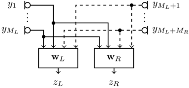
Fig. 1. Binaural hearing device configuration with M L microphones on the left side and M R microphones the right side.
<details>
<summary>Image 1 Details</summary>
### Visual Description
## Diagram: Neural Network Layer
### Overview
The image is a diagram representing a layer in a neural network, specifically showing how inputs are processed by two weight matrices, W_L and W_R, to produce outputs z_L and z_R. The diagram illustrates the connections between input nodes (y_1 to y_{M_L} and y_{M_L+1} to y_{M_L+M_R}) and the weight matrices.
### Components/Axes
* **Input Nodes:**
* `y_1`: Top-left input node.
* `y_{M_L}`: Bottom-left input node.
* `y_{M_L+1}`: Top-right input node.
* `y_{M_L+M_R}`: Bottom-right input node.
* **Weight Matrices:**
* `W_L`: Left weight matrix (rectangular box).
* `W_R`: Right weight matrix (rectangular box).
* **Output Nodes:**
* `z_L`: Output from the left weight matrix.
* `z_R`: Output from the right weight matrix.
* **Connections:**
* Solid lines: Connections from the left input nodes to both weight matrices.
* Dashed lines: Connections from the right input nodes to both weight matrices.
### Detailed Analysis
* **Input Nodes:** The input nodes are represented as circles. The left input nodes range from `y_1` to `y_{M_L}`, and the right input nodes range from `y_{M_L+1}` to `y_{M_L+M_R}`.
* **Weight Matrices:** The weight matrices `W_L` and `W_R` are represented as rectangular boxes.
* **Connections:**
* The solid lines indicate connections from the left input nodes (`y_1` to `y_{M_L}`) to both `W_L` and `W_R`. Specifically, two solid lines connect to `W_L` and two solid lines connect to `W_R`.
* The dashed lines indicate connections from the right input nodes (`y_{M_L+1}` to `y_{M_L+M_R}`) to both `W_L` and `W_R`. Specifically, two dashed lines connect to `W_L` and two dashed lines connect to `W_R`.
* **Output Nodes:** The outputs `z_L` and `z_R` are represented as arrows pointing downwards from the weight matrices `W_L` and `W_R`, respectively.
### Key Observations
* The diagram shows a fully connected layer where both `W_L` and `W_R` receive inputs from both the left and right input node groups.
* The use of solid and dashed lines differentiates the origin of the inputs (left vs. right).
* The diagram suggests that the outputs `z_L` and `z_R` are calculated based on the weighted sum of the inputs, using the weight matrices `W_L` and `W_R`, respectively.
### Interpretation
The diagram illustrates a layer in a neural network where inputs are processed by two weight matrices. The inputs are divided into two groups, and each weight matrix receives inputs from both groups. This type of architecture can be used for various purposes, such as feature extraction or dimensionality reduction. The connections between the input nodes and the weight matrices determine how the inputs are combined to produce the outputs. The diagram highlights the flow of information through the layer and the role of the weight matrices in transforming the inputs.
</details>
## II. HEARING DEVICE CONFIGURATION
In Section II-A the considered binaural hearing device configuration and the signal model are introduced. In Sections II-B and II-C the objective performance measures and the binaural cues are defined.
## A. Signal Model
Consider the binaural hearing device configuration depicted in Figure 1 with M L microphones on the left side and M R microphones on the right side, i.e., M = M L + M R microphones in total. In this paper we consider an acoustic scenario with one desired source (target speaker) and one interfering source (competing speaker) in a noisy and reverberant environment, where the background noise is assumed to be incoherent (e.g., diffuse babble noise, sensor noise).
In the frequency-domain, the m -th microphone signal y m ( ω ) can be decomposed as
<!-- formula-not-decoded -->
with ω the normalized (radian) frequency, x m ( ω ) the desired source component, u m ( ω ) the interfering source component and n m ( ω ) the noise component in the m -th microphone signal. The undesired component v m ( ω ) is defined as the sum of the interfering source component u m ( ω ) and the noise component n m ( ω ) . For the sake of conciseness, we omit the variable ω in the remainder of the paper wherever possible. The M -dimensional noisy input vector containing all microphone signals is defined as
<!-- formula-not-decoded -->
where ( · ) T denotes the transpose. Using (1), this vector can be written as
<!-- formula-not-decoded -->
where x , u , n and v are defined similarly as y in (2).
<!-- formula-not-decoded -->
For the considered acoustic scenario, the desired source component and the interfering source component can be written as where s x and s u denote the desired source signal and the interfering source signal, respectively, and a and b denote M -dimensional ATF vectors, containing the ATFs between the microphones and the desired source and the interfering source, respectively. It should be noted that the ATFs include reverberation, microphone characteristics and the head-shadow effect.
Without loss of generality, the first microphone on each side is defined as the so-called reference microphone. To simplify the notation, the reference microphone signals y 1 and y M L +1 are denoted as y L and y R , i.e.,
<!-- formula-not-decoded -->
where e L and e R denote M -dimensional selection vectors with all elements equal to 0 except one element equal to 1, i.e., e L (1) = 1 and e R ( M L +1) = 1 . Using (3), (4) and (5), the reference microphone signals can be written as
<!-- formula-not-decoded -->
The noisy input covariance matrix R y , the desired source covariance matrix R x , the interfering source covariance matrix R u and the noise covariance matrix R n are defined as
<!-- formula-not-decoded -->
<!-- formula-not-decoded -->
<!-- formula-not-decoded -->
with E{·} the expected value operator and ( · ) H the conjugate transpose. Assuming statistical independence between all signal components, R y can be written as
<!-- formula-not-decoded -->
with R v the undesired covariance matrix. Using (4), (8) and (9), the desired source covariance matrix and the interfering source covariance matrix can be written as rank-1 matrices, i.e.,
<!-- formula-not-decoded -->
with p x = E{| s x | 2 } the PSD of the desired source and p u = E{| s u | 2 } the PSD of the interfering source. The noise covariance matrix R n is assumed to be full-rank, i.e., invertible and positive definite.
The left and the right output signals z L and z R are obtained by filtering and summing all microphone signals using the M -dimensional filter vectors w L and w R (cf. Figure 1), i.e.,
<!-- formula-not-decoded -->
## B. Objective Performance Measures
The PSD and the cross power spectral density (CPSD) of the desired source component in the left and the right reference microphone signal are given by
<!-- formula-not-decoded -->
<!-- formula-not-decoded -->
<!-- formula-not-decoded -->
Similarly, the output PSD of the desired source component in the left and the right output signal is given by
<!-- formula-not-decoded -->
The same definitions can be applied for the noisy input signal, the interfering source component and the noise component by substituting R x with R y , R u or R n .
The narrowband input SNR in the left and the right reference microphone signal is defined as the ratio of the input PSD of the desired source and noise components, i.e.,
<!-- formula-not-decoded -->
Similarly, the narrowband output SNR in the left and the right output signal is defined as the ratio of the output PSD of the desired source and noise components, i.e.,
<!-- formula-not-decoded -->
The SNR improvement (in dB) is defined as ∆SNR L/R = 10 log 10 SNR out L/R -10 log 10 SNR in L/R .
The narrowband input signal-to-interference ratio (SIR) in the left and the right reference microphone signal is defined as the ratio of the input PSD of the desired source and interfering source components, i.e.,
<!-- formula-not-decoded -->
Similarly, the narrowband output SIR in the left and the right output signal is defined as the ratio of the output PSD of the desired source and interfering source components, i.e.,
<!-- formula-not-decoded -->
The SIR improvement (in dB) is defined as ∆SIR L/R = 10 log 10 SIR out L/R -10 log 10 SIR in L/R .
## C. Binaural Cues
For coherent sources (desired source and interfering source) the main binaural cues used by the auditory system are the ILD and the ITD [4], which can be computed from the so-called interaural transfer function (ITF). Using (11), the input ITFs of the desired source and the interfering source are given by [11]
<!-- formula-not-decoded -->
<!-- formula-not-decoded -->
Similarly, the output ITFs of the desired source and the interfering source are given by
<!-- formula-not-decoded -->
<!-- formula-not-decoded -->
The ILD and the ITD can be calculated from the ITF as [11]
<!-- formula-not-decoded -->
with ∠ ( · ) denoting the unwrapped phase.
For an incoherent sound field (background noise), ILD and ITD cues are not very descriptive, but the IC is known to play a major role for spatial perception (e.g., spatial width or diffuseness) [4]. The input IC of the noise component is defined as
<!-- formula-not-decoded -->
while the output IC of the noise component is defined as
<!-- formula-not-decoded -->
Because the IC is typically complex-valued, the magnitudesquared coherence (MSC) is often used. The input and the output MSC of the noise component are defined as
<!-- formula-not-decoded -->
An MSC of 1 corresponds to a coherent source perceived as a distinct point source, while smaller MSC values correspond to a broader or even diffuse sound field impression [4].
## III. BINAURAL BEAMFORMING ALGORITHMS
In this section we briefly review three state-of-the-art binaural beamforming algorithms, namely the BMVDR beamformer, the BLCMV beamformer and the BMVDR-N beamformer. We discuss the performance of these beamforming algorithms in terms of noise and interference reduction performance and binaural cue preservation. For the sake of conciseness, we only show expressions for the left hearing device, denoted by the subscript L . It should be noted that all expressions can also be formulated for the right hearing device by changing the subscript to R .
## A. BMVDR Beamformer
The BMVDR aims at minimizing the output PSD of the noise component while preserving the desired source component in the reference microphone signals [2], [3], [11]. The constrained optimization problem for the left filter vector is given by
<!-- formula-not-decoded -->
Using (4), (6) and (9), the solution of (28) is equal to [2], [22], [23]
<!-- formula-not-decoded -->
with
<!-- formula-not-decoded -->
It should be noted that the BMVDR can also be defined using the undesired covariance matrix R v instead of the noise covariance matrix R n . However, since R v is considerably more difficult to estimate or model in practice than R n , in this paper we only consider the BMVDR using R n in (29).
By substituting (29) in (18) and (20), it has been shown in [3], [11] that the output SNR and the output SIR of the BMVDR are equal to
<!-- formula-not-decoded -->
<!-- formula-not-decoded -->
with γ a defined in (30) and
<!-- formula-not-decoded -->
Although the BMVDR yields the largest output SNR among all distortionless binaural beamforming algorithms, the output SIR depends on the relative position of the interfering source to the desired source, cf. (33).
As shown in [3], [11], [13], the BMVDR preserves the binaural cues of the desired source, i.e.,
<!-- formula-not-decoded -->
but distorts the binaural cues of the undesired sources, i.e., for the interfering source
<!-- formula-not-decoded -->
and for the background noise
<!-- formula-not-decoded -->
Hence, at the output of the BMVDR the interfering source and the (incoherent) background noise are perceived as coming from the direction of the desired source, which is obviously undesired in terms of spatial awareness.
## B. BLCMV Beamformer
In addition to preserving the desired source component in the reference microphone signals, the BLCMV preserves a scaled version of the interfering source component in the reference microphone signals while minimizing the output PSD of the noise component [12], [14]. The constrained optimization problem for the left filter vector is given by [14]
<!-- formula-not-decoded -->
with 0 < δ ≤ 1 the (real-valued) interference scaling parameter. Using (4), (6) and (9), the solution of (37) is equal to [14]
<!-- formula-not-decoded -->
with the constraint matrix C and the left response vector g L defined as
<!-- formula-not-decoded -->
By substituting (38) in (18), it has been shown in [14] that the output SNR of the BLCMV is equal to
<!-- formula-not-decoded -->
with
<!-- formula-not-decoded -->
where {·} denotes the real part of a complex number. The output SNR of the BLCMV in (40) is smaller than or equal to the output SNR of the BMVDR in (31), since less degrees of freedom are available for noise reduction. In addition, the output SIR of the BLCMV is equal to [14]
<!-- formula-not-decoded -->
which can hence be directly controlled by the interference scaling parameter δ .
As shown in [14], the BLCMV preserves the binaural cues of both the desired source and the interfering source, i.e.,
<!-- formula-not-decoded -->
<!-- formula-not-decoded -->
and the output MSC of the noise component is equal to
<!-- formula-not-decoded -->
Because R xu, 1 in (41) is a rank-2 matrix, it has been shown in [14] that the output MSC of the noise component is smaller than 1 but is not equal to the input MSC of the noise component. Furthermore, it should be noted that the output MSC of the noise component depends on the relative position of the interfering source to the desired source, cf. (41) and (42), such that it is not straightforward to control the binaural cues of the background noise.
## C. BMVDR-N beamformer
In addition to preserving the desired source component in the reference microphone signals, the BMVDR with partial noise estimation (BMVDR-N) aims at preserving a scaled version of the noise component in the reference microphone signals [3], [10], [11]. The constrained optimization problem for the left filter vector is given by
<!-- formula-not-decoded -->
with 0 ≤ η ≤ 1 the (real-valued) mixing parameter. It has been shown in [11] that the solution of (47) is equal to
<!-- formula-not-decoded -->
with w BMVDR ,L defined in (29). Hence, the output signals of the BMVDR-N can be interpreted as a mixture between the noisy reference microphone signals (scaled with η ) and the output signals of the BMVDR (scaled with 1 -η ). For η = 0 , the BMVDR-N is equal to the BMVDR, whereas for η = 1 , no beamforming is applied.
Since the output signals of the BMVDR are mixed with the noisy reference microphone signals, the output SNR of the BMVDR-N is always smaller than or equal to the output SNR of the BMVDR [11], i.e.,
<!-- formula-not-decoded -->
and decreases with increasing η . By substituting (48) in (20), it can be shown that the output SIR of the BMVDR-N is equal to with
<!-- formula-not-decoded -->
As shown in [11], [16], the BMVDR-N preserves the binaural cues of the desired source, i.e.,
<!-- formula-not-decoded -->
By substituting (48) in (24) and (26), it has been shown in [16] and [20] that the output ITF of the interfering source is equal to
<!-- formula-not-decoded -->
and the output MSC of the noise component is equal to
<!-- formula-not-decoded -->
It can be seen from (52) and (53) that only for η = 1 the binaural cues of the undesired sources (interfering source and background noise) are preserved, whereas for η = 0 the binaural cues of the undesired sources are equal to the binaural cues of the desired source (as for the BMVDR). The mixing parameter η hence allows to trade off between noise reduction performance and binaural cue preservation of the background noise, or in other words control the binaural cues of the background noise. Furthermore, it should be noted that the interference reduction performance in (50) and the output ITF of the interfering source in (52) do not only depend on the mixing parameter η but also on the relative position of the interfering source to the desired source, such that it is not straightforward to control both.
## IV. BLCMV WITH PARTIAL NOISE ESTIMATION
Aiming at merging the advantages of the BLCMV and the BMVDR-N, i.e., preserving the binaural cues of the interfering source and controlling the binaural cues of the background noise, in Section IV-A we present the BLCMV beamformer with partial noise estimation (BLCMV-N). Similarly as for the BLCMV in [14], in Sections IV-B and IV-C we derive two decompositions for the BLCMV-N which reveal differences and similarities between the BLCMV-N and the BLCMV.
<!-- formula-not-decoded -->
## A. BLCMV-N Beamformer
Compared to the BMVDR in (28), the BLCMV-N uses an additional constraint to preserve a scaled version of the interfering source component in the reference microphone signals, like the BLCMV in (37), and aims at preserving a scaled version of the noise component in the reference microphone signals, like the BMVDR-N in (47). The constrained optimization problem for the left filter vector is given by
<!-- formula-not-decoded -->
The solution of (54) is equal to (see Appendix A)
<!-- formula-not-decoded -->
with C defined in (39) and the adjusted interference scaling parameter ¯ δ equal to
<!-- formula-not-decoded -->
<!-- formula-not-decoded -->
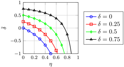
Hence, the output signals of the BLCMV-N can be interpreted as a mixture between the noisy reference microphone signals (scaled with η ) and the output signals of a BLCMV (scaled with 1 -η ) using the adjusted interference scaling parameter ¯ δ in (56) instead of the interference scaling parameter δ . For η = 0 , the BLCMV-N is equal to the BLCMV in (38) with ¯ δ = δ , whereas for η = 1 , it should be realized that only if δ = 1 no beamforming is applied. Since mixing with the reference microphone signals not only affects the noise component but also the interfering source component, the adjusted interference scaling parameter ¯ δ depends on both the interference scaling parameter δ as well as the mixing parameter η due to the interference reduction constraint in (54). Figure 2 depicts ¯ δ as a function of η for different values of δ . It can be seen that
As will be shown in more detail in the following sections, using the parameters δ and η it is possible to control the noise reduction performance, the interference reduction performance and the binaural cues of the background noise for the BLCMVN.
## B. Decomposition into two BLCMVs
In [14] it has been shown that the BLCMV in (38) can be decomposed as the sum of two sub-BLCMVs, i.e.,
<!-- formula-not-decoded -->
with
<!-- formula-not-decoded -->
<!-- formula-not-decoded -->
JOURNAL OF L A T E X CLASS FILES, VOL. 14, NO. 8, AUGUST 2015
Fig. 2. Adjusted interference scaling parameter ¯ δ as a function of η for different values of δ . Fig. 2. Adjusted interference scaling parameter ¯ δ as a function of η for different values of δ .
<details>
<summary>Image 2 Details</summary>
### Visual Description
## Chart: Plot of Delta-Bar vs. Eta for Different Delta Values
### Overview
The image is a 2D plot showing the relationship between two variables, delta-bar (δ̄) on the y-axis and eta (η) on the x-axis, for four different values of delta (δ): 0, 0.25, 0.5, and 0.75. Each delta value is represented by a different colored line with a distinct marker.
### Components/Axes
* **X-axis:** η (eta), ranging from 0 to 1 in increments of 0.2.
* **Y-axis:** δ̄ (delta-bar), ranging from -1 to 1 in increments of 0.5.
* **Legend:** Located on the right side of the plot, it identifies each line by its color, marker, and corresponding delta value:
* Blue line with circle markers: δ = 0
* Red line with square markers: δ = 0.25
* Green line with diamond markers: δ = 0.5
* Black line with triangle markers: δ = 0.75
### Detailed Analysis
* **δ = 0 (Blue, Circles):** The line starts at approximately (0, 0) and decreases to approximately (0.6, -1).
* **δ = 0.25 (Red, Squares):** The line starts at approximately (0, 0.25) and decreases to approximately (0.7, -1).
* **δ = 0.5 (Green, Diamonds):** The line starts at approximately (0, 0.5) and decreases to approximately (0.8, -0.9).
* **δ = 0.75 (Black, Triangles):** The line starts at approximately (0, 0.75) and decreases to approximately (0.9, -0.9).
Here's a breakdown of approximate data points for each series:
* **δ = 0 (Blue, Circles):**
* (0, 0)
* (0.2, -0.25)
* (0.4, -0.6)
* (0.6, -1)
* **δ = 0.25 (Red, Squares):**
* (0, 0.25)
* (0.2, 0.1)
* (0.4, -0.25)
* (0.6, -0.9)
* **δ = 0.5 (Green, Diamonds):**
* (0, 0.5)
* (0.2, 0.45)
* (0.4, 0.2)
* (0.6, -0.5)
* (0.8, -0.9)
* **δ = 0.75 (Black, Triangles):**
* (0, 0.75)
* (0.2, 0.7)
* (0.4, 0.6)
* (0.6, 0.4)
* (0.8, 0)
* (0.9, -0.9)
### Key Observations
* As η increases, δ̄ generally decreases for all values of δ.
* For a given value of η, as δ increases, δ̄ also tends to increase.
* The curves become steeper as δ decreases.
### Interpretation
The plot illustrates the relationship between δ̄ and η for different values of δ. The data suggests that increasing δ shifts the curve upwards, indicating a positive correlation between δ and δ̄. The negative slope of each curve indicates an inverse relationship between η and δ̄. The varying steepness of the curves suggests that the sensitivity of δ̄ to changes in η depends on the value of δ.
</details>
A. BLCMV-N Beamformer and the respective response vectors
Compared interfering source component in the reference microphone signals, like the BLCMV beamformer in (38), and aims at preserving a scaled version of the noise component in the reference microphone signals, like the BMVDR-N in (48). The constrained optimization problem for the left filter vector is given by The sub-BLCMV w x,L in (59) preserves the desired source component in the reference microphone signals and steers a null towards the interfering source, whereas the sub-BLCMV w u,L in (60) preserves the interfering source component in the reference microphone signals and steers a null towards the desired source. Using (55), it can be easily seen that the proposed BLCMV-N can be decomposed as
<!-- formula-not-decoded -->
an additional
<!-- formula-not-decoded -->
as a mixture between the noisy reference microphone signals
The solution of (56) is equal to (see Appendix for derivation) w BLCMV -N ,L = η e L +(1 -η ) R -1 n C ( C H R -1 n C ) -1 [ a ∗ L ¯ δb ∗ L ] (57) with C defined in (40) and the adjusted interference scaling parameter ¯ δ equal to ¯ δ = δ -η 1 -η . (58) The output signals of the BLCMV-N hence can be interpreted Hence, the BLCMV-N can be interpreted as a mixture of the reference microphone signals (scaled with η ), a BLCMV that preserves the desired source and rejects the interfering source (scaled with 1 -η ) and a BLCMV that preserves the interfering source and rejects the desired source (scaled with δ -η ). Since the scaling of the sub-BLCMV w x,L controls the desired source component without affecting the interfering source component and the scaling of the sub-BLCMV w u,L controls the interfering source component without affecting the desired source component [14], it can be directly observed from the scaling factors in (62) that the desired source component is not distorted and the interfering source component is scaled with δ .
## (scaled with η ) and the output signals of a BLCMV (scaled C. Decomposition using Binauralization Postfilters
and the
<!-- formula-not-decoded -->
with 1 -η ) using the adjusted interference scaling parameter ¯ δ in (58) instead of the interference scaling parameter δ . For η = 0 , the BLCMV-N is equal to the BLCMV in (39) with ¯ δ = δ , whereas for η = 1 , no beamforming is applied. Since mixing with the reference microphone signals not only affects the noise component but also the interfering source component In [14] it has also been shown that the sub-BLCMV w x,L in (59) for the left hearing device and the sub-BLCMV w x,R for the right hearing device (defined similarly as w x,L ) can be written using a common spatial filter and two binauralization postfilters as
¯
<!-- formula-not-decoded -->
to be satisfied, the adjusted interference scaling parameter δ depends on both the interference scaling parameter δ as well with the common desired BLCMV (D-BLCMV) given by
¯ δ ( η, δ ) = > 0 , for δ > η < 0 , for δ < η 0 , for δ = η . (59) and the ATFs a L and a R between the desired source and the reference microphones used as binauralization postfilters. Similarly, the sub-BLCMV w u,L in (60) and the sub-BLCMV w u,R (defined similarly as w u,L ) can be written as w u,L = w u b ∗ L , w u,R = w u b ∗ R , (65)
B. Deco
Simila reference
BLCMV
different
BLCMV
w
BLC
with the and their
The sub- and steer
desired s rejection
microph preserves
It can th
Hence, t that
the refer
interferin pres
BLCMV
combinat rejects
t
binaural partially
interferin
BLCMV
Section cues of t
C.
Filter
For a was sho
bines bot be writte
interferin
BLCMV
with the
desir desired s
binaurali
<details>
<summary>Image 3 Details</summary>
### Visual Description
## Diagram: Signal Processing Flow
### Overview
The image depicts a signal processing diagram, likely related to audio processing or beamforming. It shows how an input signal 'y' is processed through various stages involving weighting, conjugation, multiplication, and summation to produce two output signals, 'zL' and 'zR'.
### Components/Axes
* **Input Signal:** 'y'
* **Weighting Blocks:** 'wX', 'wU'
* **Error Signals:** 'eL', 'eR'
* **Conjugation Blocks:** 'a*L', 'b*L', 'a*R', 'b*R' (The asterisk denotes complex conjugation)
* **Multiplication Blocks:** Represented by the 'x' symbol inside a circle.
* **Summation Blocks:** Represented by the '+' symbol inside a circle.
* **Output Signals:** 'zL', 'zR'
* **Parameters:** 'η' (eta), 'δ' (delta)
### Detailed Analysis
1. **Input Signal 'y':** The input signal 'y' is split into three paths.
2. **Top Path:** 'y' is connected to 'wX' and 'wU'.
3. **Error Signal Paths:** 'eL' and 'eR' are directly fed into the processing chain.
4. **Weighting and Conjugation:**
* 'wX' is connected to 'a*L' and 'a*R'.
* 'wU' is connected to 'b*L' and 'b*R'.
5. **Multiplication:**
* 'eL' is multiplied by 'η'.
* 'a*L' is multiplied by '1-η'.
* 'b*L' is multiplied by 'δ-η'.
* 'a*R' is multiplied by '1-η'.
* 'b*R' is multiplied by 'δ-η'.
* 'eR' is multiplied by 'η'.
6. **Summation:**
* The outputs of 'eL * η', 'a*L * (1-η)', and 'b*L * (δ-η)' are summed to produce 'zL'.
* The outputs of 'a*R * (1-η)', 'b*R * (δ-η)', and 'eR * η' are summed to produce 'zR'.
### Key Observations
* The diagram shows a parallel processing structure for generating two output signals.
* The parameters 'η' and 'δ' control the weighting of different components in the summation stages.
* Complex conjugation is applied to the outputs of the weighting blocks 'wX' and 'wU'.
### Interpretation
The diagram likely represents a system for adaptive signal processing, possibly for spatial audio or noise cancellation. The input signal 'y' is processed through weighted paths, and error signals 'eL' and 'eR' are used to refine the output signals 'zL' and 'zR'. The parameters 'η' and 'δ' likely control the adaptation rate or the balance between different signal components. The complex conjugation suggests that the system operates on complex-valued signals, which is common in signal processing applications. The structure suggests a form of beamforming or spatial filtering, where the outputs 'zL' and 'zR' represent signals from different spatial locations or channels.
</details>
×
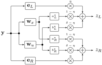
Fig. 3. Decomposition of the BLCMV-N into a mixture of the reference microphone signals and two BLCMVs with binauralization postfilters.
with the common interference BLCMV (I-BLCMV) given by and the ATFs b L and b R between the interfering source and the reference microphones used as binauralization postfilters.
<!-- formula-not-decoded -->
Using (63) and (65) in (62), the BLCMV-N can be decomposed as
<!-- formula-not-decoded -->
<!-- formula-not-decoded -->
Figure 3 depicts this decomposition of the BLCMV-N using common spatial filters and binauralization postfilters. The output signals of the BLCMV-N can hence be interpreted as a mixture between the reference microphone signals (scaled with η ), the binauralized output signals of the D-BLCMV (scaled with 1 -η ) and the binauralized output signals of the I-BLCMV (scaled with δ -η ).
Due to the constraints in (54), the BLCMV-N perfectly preserves the desired source component and scales the interfering source component with δ . Using (67) and (68), the noise component in the output signals of the BLCMV-N are equal to
<!-- formula-not-decoded -->
with n x = w H x n and n u = w H u n the noise component in the output signal of the D-BLCMV and the I-BLCMV, respectively. The noise component in the output signals of the BLCMV-N can hence be interpreted as a mixture between the noise component in the reference microphone signals (scaled with η ), a coherent residual noise source ( n x ) coming from the direction of the desired source (scaled with 1 -η ) and a coherent residual noise source ( n u ) coming from the direction of the interfering source (scaled with δ -η ).
## V. PERFORMANCE OF THE BLCMV-N
In this section we provide a performance analysis of the proposed BLCMV-N. In Section V-A we derive the output PSDs of the signal components. In Sections V-B and V-C
we analyze the noise and interference reduction performance and the binaural cue preservation performance. Finally, in Section V-D we discuss the setting of the mixing parameter η and the interference scaling parameter δ .
## A. Output Power Spectral Densities
Due to the constraints in (54), the output PSD of the desired and interfering source components in the left output signal of the BLCMV-N are equal to, cf. (13),
<!-- formula-not-decoded -->
<!-- formula-not-decoded -->
Furthermore, the output PSD of the noise component in the left output signal of the BLCMV-N is equal to (see Appendix B)
with
<!-- formula-not-decoded -->
with γ a defined in (30), γ ab defined in (33), and γ b and Ψ defined in (42). It can be seen that the output PSD of the noise component for the BLCMV-N is a quadratic function in both the mixing parameter η and the interference scaling parameter δ . By comparing (74) to (41), it can be observed that
<!-- formula-not-decoded -->
<!-- formula-not-decoded -->
where R δ =1 xu, 1 denotes the expression for the BLCMV in (41) with δ = 1 , corresponding to no suppression of the interfering source. Please note that for η = 0 , R xu, 3 = R xu, 1 , and for η = 1 and δ = 1 , R xu, 3 = 0 M . By using (75) in (73), it follows that
<!-- formula-not-decoded -->
## B. Noise and Interference Reduction Performance
By substituting (71) and (73) in (18), the left output SNR of the BLCMV-N is equal to
<!-- formula-not-decoded -->
which depends on both the mixing parameter η and the interference scaling parameter δ . Using (76) and realizing that the output PSD of the noise component in the left output signal of the BLCMV (for any value of δ ) is smaller than or equal to the PSD of the noise component in the left reference microphone signal, the output SNR of the BLCMV-N in (77) is smaller than or equal to the output SNR of the BLCMV in (40), i.e.,
<!-- formula-not-decoded -->
By substituting (71) and (72) in (20), the left output SIR of the BLCMV-N is equal to
<!-- formula-not-decoded -->
which is equal to the left output SIR of the BLCMV in (43) and solely controlled by the interference scaling parameter δ . For η = 0 , the left output SNR of the BLCMV-N is equal to the left output SNR of the BLCMV in (40), while for η = 1 and δ = 1 , the left output SNR of the BLCMV-N is equal to the left input SNR because no beamforming is applied.
## C. Binaural Cue Preservation
Similarly as for the BLCMV, due to the constraints in (54) the BLCMV-N preserves the binaural cues of both the desired source and the interfering source, i.e.,
<!-- formula-not-decoded -->
<!-- formula-not-decoded -->
Using (26), the output IC of the noise component for the BLCMV-N is equal to (see Appendix B for derivation of components)
<!-- formula-not-decoded -->
with R xu, 3 defined in (74). Since R xu, 3 depends on both the mixing parameter η and the interference scaling parameter δ , also the output IC of the noise component in (82) depends on both parameters. Using (27), the output MSC of the noise component for the BLCMV-N is equal to
<!-- formula-not-decoded -->
Since for η = 0 the BLCMV-N is equal to the BLCMV, the output MSC of the noise component is smaller than 1, see Section III-B. It should however be realized that in contrast to the BMVDR-N discussed in Section III-C, for η = 1 the BLCMV-N does not always preserve the MSC of the noise component. Only for η = 1 and δ = 1 the binaural cues of all signal components are preserved because no beamforming is applied.
## D. Parameter Settings
Maximizing the left output SNR in (77) corresponds to minimizing the denominator, i.e., using (75),
Setting the derivative of (84) with respect to the mixing parameter η equal to zero, yields
<!-- formula-not-decoded -->
<!-- formula-not-decoded -->
as the optimal mixing parameter η in terms of left (and right) output SNR. The derivative of (84) with respect to the interference scaling parameter δ is equal to, using (41),
<!-- formula-not-decoded -->
Setting (86) to zero and solving for δ yields the optimal interference scaling parameter in terms of left output SNR, i.e., with
As can be seen from (79), the output SIR is not affected by the mixing parameter η but is solely determined by the interference scaling parameter δ .
<!-- formula-not-decoded -->
<!-- formula-not-decoded -->
## VI. SIMULATIONS
In Section VI-A we first validate the expressions derived in the previous sections using measured anechoic ATFs. In Section VI-B we then experimentally compare the performance of the proposed BLCMV-N with the BMVDR, BLCMV and BMVDR-N using recorded signals in a reverberant environment with a competing speaker and multi-talker babble noise. Finally, in Section VI-C we compare the spatial impression of the considered binaural beamforming algorithms using a perceptual listening test.
## A. Validation Using Measured Anechoic ATFs
To validate the derived expressions for the considered algorithms we used measured anechoic ATFs of two behind-the-ear hearing aids mounted on a head-and-torso-simulator (HATS) [24]. Each hearing aid has two microphones ( M = 4 ) with an inter-microphone distance of about 14 mm . We chose the front microphone on each hearing aid as reference microphone. The ATFs were calculated from anechoic impulse responses using a 512-point FFT at a sampling rate of 16 kHz .
The desired source was placed at 0 ◦ (in front) and the interfering source was placed at -35 ◦ (to the left), both at a distance of 3 m from the HATS. The desired source covariance matrix R x and the interfering source covariance matrix R u were constructed using the ATF vector of the desired source a and the ATF vector of the interfering source b according to (11), where the PSD of the desired source p x and the PSD of the interfering source p u were both set to 1. As background noise we considered a combination of spatially white and cylindrically isotropic noise, i.e., the noise covariance matrix R n was constructed as
<!-- formula-not-decoded -->
with p n, w the PSD of the spatially white noise, I M the M × M -dimensional identity matrix, p n, cyl the PSD of the cylindrically isotropic noise and Γ its spatial coherence matrix. The ( i, j ) -th element of the spatial coherence matrix Γ was calculated using all available anechoic ATFs as with h ( θ k ) the anechoic ATF at angle θ k and K the total number of angles in the database ( K = 72 for [24]). The PSD of the spatially white noise p n, w was set to -55 dB , while the PSD of the cylindrically isotropic noise p n, cyl was set to 1.
<!-- formula-not-decoded -->
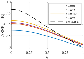
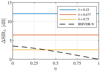
Fig. 4. SNR improvement for the BLCMV-N and the BMVDR-N at 500Hz .
<details>
<summary>Image 4 Details</summary>
### Visual Description
## Chart: Delta SNR vs. Eta
### Overview
The image is a line chart comparing the change in Signal-to-Noise Ratio (ΔSNR_L) in decibels (dB) as a function of a variable η. There are four solid lines representing different values of δ (0.01, 0.25, 0.477, and 0.75) and one dashed line representing BMVDR-N. The chart shows how ΔSNR_L changes as η increases from 0 to 1.
### Components/Axes
* **X-axis (Horizontal):** η, ranging from 0 to 1 in increments of 0.25.
* **Y-axis (Vertical):** ΔSNR_L [dB], ranging from 0 to 10 in increments of 2.5.
* **Legend (Top-Right):**
* Blue line: δ = 0.01
* Orange line: δ = 0.25
* Yellow line: δ = 0.477
* Purple line: δ = 0.75
* Black dashed line: BMVDR-N
### Detailed Analysis
* **Blue line (δ = 0.01):** Starts at approximately 3.7 dB at η = 0 and decreases to approximately 0 dB at η = 1. The line slopes downward consistently.
* **Orange line (δ = 0.25):** Starts at approximately 6.2 dB at η = 0 and decreases to approximately 0.2 dB at η = 1. The line slopes downward consistently.
* **Yellow line (δ = 0.477):** Starts at approximately 6.8 dB at η = 0 and decreases to approximately 0.2 dB at η = 1. The line slopes downward consistently.
* **Purple line (δ = 0.75):** Starts at approximately 6.2 dB at η = 0 and decreases to approximately 0 dB at η = 1. The line slopes downward consistently.
* **Black dashed line (BMVDR-N):** Starts at approximately 8.8 dB at η = 0 and decreases to approximately 0 dB at η = 1. The line slopes downward consistently.
### Key Observations
* All lines show a decreasing trend in ΔSNR_L as η increases.
* The BMVDR-N (black dashed line) consistently has the highest ΔSNR_L for any given value of η.
* The lines for δ = 0.25, δ = 0.477, and δ = 0.75 are very close to each other.
* The line for δ = 0.01 has the lowest ΔSNR_L for any given value of η.
### Interpretation
The chart illustrates the relationship between ΔSNR_L and η for different values of δ and the BMVDR-N method. The decreasing trend suggests that as η increases, the improvement in SNR decreases. The BMVDR-N method consistently outperforms the other methods (different δ values) in terms of ΔSNR_L. The proximity of the lines for δ = 0.25, δ = 0.477, and δ = 0.75 suggests that the value of δ has a diminishing effect on ΔSNR_L beyond a certain point. The data suggests that BMVDR-N is the preferred method for maximizing the change in SNR.
</details>
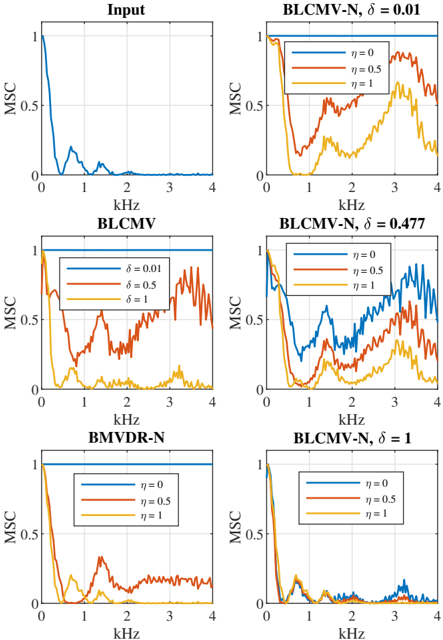
Fig. 5. SIR improvement for the BLCMV-N and the BMVDR-N at 500Hz .
<details>
<summary>Image 5 Details</summary>
### Visual Description
## Line Chart: Delta SIR_L vs. Eta
### Overview
The image is a line chart displaying the relationship between Delta SIR_L (in dB) and Eta (η). There are four data series represented by different colored lines: blue (δ = 0.25), red (δ = 0.477), yellow (δ = 0.75), and a black dashed line (BMVDR-N). The chart shows how Delta SIR_L changes with respect to Eta for different values of δ and for the BMVDR-N method.
### Components/Axes
* **X-axis (Horizontal):** Eta (η), ranging from 0 to 1 in increments of 0.25.
* **Y-axis (Vertical):** Delta SIR_L (ΔSIR_L) in dB, ranging from 0 to 15 in increments of 5.
* **Legend:** Located in the top-right corner of the chart.
* Blue line: δ = 0.25
* Red line: δ = 0.477
* Yellow line: δ = 0.75
* Black dashed line: BMVDR-N
### Detailed Analysis
* **Blue Line (δ = 0.25):** This line is horizontal, indicating a constant value of Delta SIR_L across all values of Eta. The value is approximately 12 dB.
* **Red Line (δ = 0.477):** This line is also horizontal, indicating a constant value of Delta SIR_L across all values of Eta. The value is approximately 7 dB.
* **Yellow Line (δ = 0.75):** This line is horizontal, indicating a constant value of Delta SIR_L across all values of Eta. The value is approximately 2 dB.
* **Black Dashed Line (BMVDR-N):** This line slopes downward, indicating a decreasing value of Delta SIR_L as Eta increases.
* At η = 0, Delta SIR_L is approximately 4 dB.
* At η = 0.25, Delta SIR_L is approximately 3 dB.
* At η = 0.5, Delta SIR_L is approximately 2 dB.
* At η = 0.75, Delta SIR_L is approximately 1 dB.
* At η = 1, Delta SIR_L is approximately 0.5 dB.
### Key Observations
* The Delta SIR_L values for fixed δ (0.25, 0.477, 0.75) remain constant regardless of the Eta value.
* The BMVDR-N method shows a decreasing Delta SIR_L as Eta increases.
* The Delta SIR_L values for different δ values are distinct and do not overlap.
### Interpretation
The chart compares the performance of different configurations (δ = 0.25, 0.477, 0.75) against the BMVDR-N method in terms of Delta SIR_L as Eta varies. The constant Delta SIR_L for fixed δ values suggests that these configurations are not affected by changes in Eta. In contrast, the BMVDR-N method's performance decreases as Eta increases, indicating a sensitivity to this parameter. The higher Delta SIR_L values for lower δ values (0.25) suggest better performance compared to higher δ values (0.75). The BMVDR-N method's performance is comparable to δ = 0.75 at lower Eta values but degrades as Eta increases.
</details>
1) Noise and Interference Reduction Performance: Using (17) and (18), Figure 4 depicts the left SNR improvement at 500 Hz for the BLCMV-N for different values of the mixing parameter η and the interference scaling parameter δ and the BMVDR-N for different values of the mixing parameter η . As expected, the BMVDR (i.e., BMVDR-N for η = 0 ) yields the largest SNR improvement (cf. (78)). Since the BMVDR-N mixes the output signals of the BMVDR with the noisy reference microphone signals, it can be observed that increasing the mixing parameter η reduces the SNR improvement of the BMVDR-N compared to the BMVDR ( η = 0 ). For the BLCMV-N, both η and δ affect the SNR improvement, which is in line with (77). Similarly to the BMVDR-N, the BLCMV-N mixes the output signals of a BLCMV with the noisy reference microphone signals. Hence, it can be observed that for any value of the interference scaling parameter δ , increasing the mixing parameter η reduces the SNR improvement of the BLCMV-N compared to the BLCMV ( η = 0 ), which is in line with (78). Since less degrees of freedom are available for noise reduction, the BLCMV ( η = 0 ) yields a smaller SNR improvement compared to the BMVDR ( η = 0 ), as discussed in Section III-B. Using (87), the interference scaling parameter δ maximizing the output SNR was equal to δ opt ,L = 0 . 477 for the considered acoustic scenario. As expected, it can be observed that using δ opt ,L leads to the largest SNR improvement of all considered values of δ . For large values of the mixing parameter η , the BLCMVN yields a larger SNR improvement than the BMVDR-N. It should be noted that the exact behaviour depends on the interference scaling parameter δ and the relative position of the interfering source to the desired source.
Using (19) and (20), Figure 5 depicts the left SIR improvement at 500 Hz for the BLCMV-N for different values of the mixing parameter η and the interference scaling parameter δ
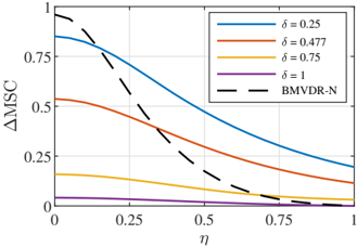
Fig. 6. The MSC of the noise component in the reference microphone signals ( Input ), in the output signals of the BLCMV for different values of the interference scaling parameter δ , the BMVDR-N for different values of the mixing parameter η and the BLCMV-N for different values of the mixing parameter η and the interference scaling paramter δ .
<details>
<summary>Image 6 Details</summary>
### Visual Description
## Chart Type: Multiple MSC vs. kHz Plots
### Overview
The image presents six plots arranged in a 2x3 grid. Each plot displays the Magnitude Squared Coherence (MSC) on the y-axis against frequency in kHz on the x-axis. The plots compare different algorithms (BLCMV, BMVDR-N, and variants) with varying parameters (δ and η).
### Components/Axes
* **Y-axis (MSC):** Ranges from 0 to 1, with a marker at 0.5.
* **X-axis (kHz):** Ranges from 0 to 4 kHz, with markers at each integer value.
* **Titles:** Each plot has a title indicating the algorithm and parameter settings.
* Top-left: "Input"
* Top-middle: "BLCMV-N, δ = 0.01"
* Top-right: "BLCMV-N, δ = 0.477"
* Middle-left: "BLCMV"
* Bottom-left: "BMVDR-N"
* Bottom-right: "BLCMV-N, δ = 1"
* **Legends:**
* BLCMV: δ = 0.01 (blue), δ = 0.5 (red), δ = 1 (yellow)
* BLCMV-N: η = 0 (blue), η = 0.5 (red), η = 1 (yellow)
* BMVDR-N: η = 0 (blue), η = 0.5 (red), η = 1 (yellow)
### Detailed Analysis
**1. Input (Top-Left)**
* Trend: The MSC starts at approximately 1, drops sharply to near 0 around 0.5 kHz, fluctuates between 0 and 0.25 until about 1.5 kHz, and then remains close to 0 for the rest of the range.
* Data Points:
* 0 kHz: ~1
* 0.5 kHz: ~0
* 1 kHz: ~0.2
* 1.5 kHz: ~0
* 4 kHz: ~0
**2. BLCMV-N, δ = 0.01 (Top-Middle)**
* Trend:
* η = 0 (blue): Stays at 1 until about 0.5 kHz, then drops to around 0.2, and rises again to fluctuate between 0.5 and 1.
* η = 0.5 (red): Stays at 1 until about 0.5 kHz, then drops to around 0.1, and rises again to fluctuate between 0.2 and 0.7.
* η = 1 (yellow): Stays at 1 until about 0.5 kHz, then drops to around 0.05, and rises again to fluctuate between 0.1 and 0.6.
* Data Points:
* η = 0 (blue): 0 kHz: 1, 0.5 kHz: ~0.2, 4 kHz: ~0.7
* η = 0.5 (red): 0 kHz: 1, 0.5 kHz: ~0.1, 4 kHz: ~0.4
* η = 1 (yellow): 0 kHz: 1, 0.5 kHz: ~0.05, 4 kHz: ~0.3
**3. BLCMV-N, δ = 0.477 (Top-Right)**
* Trend:
* η = 0 (blue): Stays at 1 until about 0.5 kHz, then drops to around 0.1, and rises again to fluctuate between 0.2 and 1.
* η = 0.5 (red): Stays at 1 until about 0.5 kHz, then drops to around 0.05, and rises again to fluctuate between 0.1 and 0.6.
* η = 1 (yellow): Stays at 1 until about 0.5 kHz, then drops to around 0, and rises again to fluctuate between 0.05 and 0.5.
* Data Points:
* η = 0 (blue): 0 kHz: 1, 0.5 kHz: ~0.1, 4 kHz: ~0.8
* η = 0.5 (red): 0 kHz: 1, 0.5 kHz: ~0.05, 4 kHz: ~0.4
* η = 1 (yellow): 0 kHz: 1, 0.5 kHz: ~0, 4 kHz: ~0.3
**4. BLCMV (Middle-Left)**
* Trend:
* δ = 0.01 (blue): Stays at 1 across the entire frequency range.
* δ = 0.5 (red): Stays at 1 until about 0.5 kHz, then drops to around 0.1, and rises again to fluctuate between 0.1 and 0.7.
* δ = 1 (yellow): Stays at 1 until about 0.5 kHz, then drops to around 0, and rises again to fluctuate between 0 and 0.4.
* Data Points:
* δ = 0.01 (blue): 0 kHz: 1, 4 kHz: 1
* δ = 0.5 (red): 0 kHz: 1, 0.5 kHz: ~0.1, 4 kHz: ~0.4
* δ = 1 (yellow): 0 kHz: 1, 0.5 kHz: ~0, 4 kHz: ~0.2
**5. BMVDR-N (Bottom-Left)**
* Trend:
* η = 0 (blue): Stays at 1 across the entire frequency range.
* η = 0.5 (red): Stays at 1 until about 0.5 kHz, then drops to around 0.05, and rises again to fluctuate between 0.1 and 0.4.
* η = 1 (yellow): Stays at 1 until about 0.5 kHz, then drops to around 0, and rises again to fluctuate between 0 and 0.2.
* Data Points:
* η = 0 (blue): 0 kHz: 1, 4 kHz: 1
* η = 0.5 (red): 0 kHz: 1, 0.5 kHz: ~0.05, 4 kHz: ~0.2
* η = 1 (yellow): 0 kHz: 1, 0.5 kHz: ~0, 4 kHz: ~0.1
**6. BLCMV-N, δ = 1 (Bottom-Right)**
* Trend:
* η = 0 (blue): Stays at 1 until about 0.5 kHz, then drops to around 0, and rises again to fluctuate between 0 and 0.2.
* η = 0.5 (red): Stays at 1 until about 0.5 kHz, then drops to around 0, and rises again to fluctuate between 0 and 0.1.
* η = 1 (yellow): Stays at 1 until about 0.5 kHz, then drops to around 0, and rises again to fluctuate between 0 and 0.1.
* Data Points:
* η = 0 (blue): 0 kHz: 1, 0.5 kHz: ~0, 4 kHz: ~0.1
* η = 0.5 (red): 0 kHz: 1, 0.5 kHz: ~0, 4 kHz: ~0.05
* η = 1 (yellow): 0 kHz: 1, 0.5 kHz: ~0, 4 kHz: ~0.05
### Key Observations
* The "Input" plot shows a significant drop in MSC around 0.5 kHz.
* For BLCMV-N and BMVDR-N, increasing η generally leads to a lower MSC across the frequency range after the initial drop.
* For BLCMV, increasing δ generally leads to a lower MSC across the frequency range after the initial drop.
* When δ = 0.01 for BLCMV, the MSC remains at 1 across the entire frequency range.
* When η = 0 for BMVDR-N, the MSC remains at 1 across the entire frequency range.
* The initial drop in MSC consistently occurs around 0.5 kHz across most plots, except for the cases where the MSC remains at 1.
### Interpretation
The plots illustrate the performance of different algorithms (BLCMV, BMVDR-N, and their variants) in terms of Magnitude Squared Coherence (MSC) across a frequency range of 0-4 kHz. The MSC measures the degree of linear relationship between two signals. A higher MSC indicates a stronger linear relationship.
The "Input" plot likely represents the MSC of the original signal before any processing. The sharp drop around 0.5 kHz suggests a significant change in the signal's characteristics at that frequency.
The other plots show how the different algorithms and parameter settings affect the MSC. The parameters δ and η appear to control the amount of noise reduction or signal modification applied by the algorithms. Increasing these parameters generally leads to a lower MSC, suggesting that the algorithms are reducing the linear coherence of the signal, possibly by removing noise or distorting the signal.
The cases where the MSC remains at 1 across the entire frequency range (BLCMV with δ = 0.01 and BMVDR-N with η = 0) likely represent scenarios where the algorithm is not applying any significant processing to the signal, thus preserving its original coherence.
The consistent drop in MSC around 0.5 kHz across most plots suggests that this frequency range is particularly sensitive to the processing applied by the algorithms.
</details>
and the BMVDR-N for different values of the mixing parameter η . As expected from (43) and (79), both the BLCMV-N and the BLCMV ( η = 0 ) yield the same SIR improvement, which is solely controlled by the interference scaling parameter δ . Hence, increasing the interference scaling parameter δ reduces the SIR improvement for both the BLCMV-N and the BLCMV. For the BMVDR-N it can be observed that increasing the mixing parameter η reduces the SIR improvement. It should be noted that the exact behaviour depends on the relative position of the interfering source to the desired source, as can be seen from (50) and (51).
2) Binaural Cue Preservation of Background Noise: For different frequencies, Figure 6 depicts the input MSC in (27) of the noise component ( Input ) and the output MSC in (27) of the noise component for the BLCMV in (46) for different values of the interference scaling parameter δ , the BMVDR-N in (53) for different values of the mixing parameter η and the BLCMV-N for different values of the mixing parameter η and the interference scaling parameter δ . Although the BLCMV is not designed to preserve the MSC of the noise component, it can be observed that an output MSC smaller than 1 is obtained, especially for large values of δ [14]. However, since the output MSC of the noise component depends on the relative position of the interfering source to the desired source, it cannot be easily controlled. Since the BMVDR-
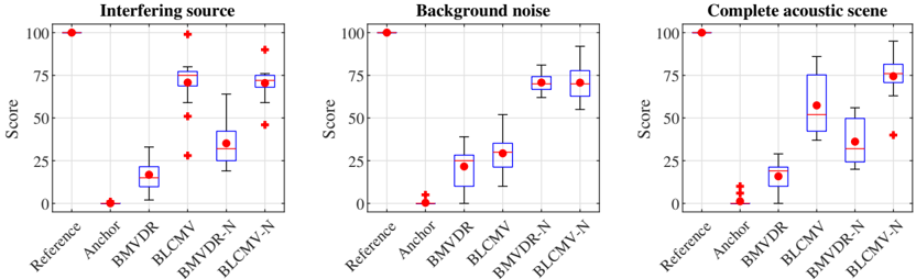
Fig. 7. Frequency-averaged MSC error of the noise component for the BLCMV-N and the BMVDR-N.
<details>
<summary>Image 7 Details</summary>
### Visual Description
## Line Chart: Delta MSC vs. Eta for Different Delta Values
### Overview
The image is a line chart showing the relationship between Delta MSC (ΔMSC) and Eta (η) for different values of Delta (δ). The chart includes multiple lines, each representing a different Delta value, and a line representing BMVDR-N. The chart illustrates how ΔMSC changes with η for each δ value and compares it to the BMVDR-N baseline.
### Components/Axes
* **Y-axis:** ΔMSC (Delta MSC), ranging from 0 to 1.0.
* Axis markers: 0, 0.25, 0.5, 0.75, 1
* **X-axis:** η (Eta), ranging from 0 to 1.0.
* Axis markers: 0, 0.25, 0.5, 0.75, 1
* **Legend:** Located in the top-right corner, identifying each line by its corresponding Delta value or as BMVDR-N.
* Blue line: δ = 0.25
* Red line: δ = 0.477
* Yellow line: δ = 0.75
* Purple line: δ = 1
* Black dashed line: BMVDR-N
### Detailed Analysis
* **Blue line (δ = 0.25):** Starts at approximately 0.85 at η = 0 and decreases to approximately 0.2 at η = 1. The line slopes downward.
* **Red line (δ = 0.477):** Starts at approximately 0.55 at η = 0 and decreases to approximately 0.05 at η = 1. The line slopes downward.
* **Yellow line (δ = 0.75):** Starts at approximately 0.25 at η = 0 and decreases to approximately 0 at η = 1. The line slopes downward.
* **Purple line (δ = 1):** Starts at approximately 0.1 at η = 0 and decreases to approximately 0 at η = 1. The line slopes downward.
* **Black dashed line (BMVDR-N):** Starts at approximately 1 at η = 0 and decreases to approximately 0 at η = 1. The line slopes downward.
### Key Observations
* As η increases, ΔMSC decreases for all values of δ.
* Higher values of δ generally correspond to lower values of ΔMSC for a given η.
* The BMVDR-N line shows a steeper decrease in ΔMSC compared to the lines representing fixed δ values.
### Interpretation
The chart illustrates the impact of Eta (η) on Delta MSC (ΔMSC) for different Delta (δ) values, and compares it to the BMVDR-N baseline. The data suggests that increasing Eta consistently reduces Delta MSC across all Delta values. The BMVDR-N line indicates a more rapid decrease in Delta MSC as Eta increases, suggesting a different relationship or sensitivity to Eta compared to the fixed Delta values. The chart demonstrates how the choice of Delta influences the relationship between Eta and Delta MSC.
</details>
N mixes the output signals of the BMVDR with the noisy reference microphone signals, it can be observed that the output MSC of the noise component is smaller than 1, and for η = 1 the MSC is perfectly preserved (but no beamforming is applied). For the BLCMV-N, it can be observed that both η and δ influence the output MSC of the noise component, as discussed in Section V-C. For η = 0 , the output MSC of the noise component for the BLCMV-N is obviously equal to the output MSC of the noise component for the BLCMV. For a fixed value of δ , it can be observed that the output MSC of the noise component approaches the input MSC of the noise component for increasing η , although it should be realized that perfect preservation of the MSC of the noise component is only possible for δ = 1 (cf. Section V-C).
For several values of the mixing parameter η , Figure 7 depicts the MSC error of the noise component for the BLCMVN and the BMVDR-N, averaged over all frequencies, i.e.,
<!-- formula-not-decoded -->
with f the frequency bin index and F the total number of frequency bins. As expected, the BMVDR ( η = 0 ) yields the largest MSC error of the noise component and increasing the mixing parameter η reduces the frequency-averaged MSC error of the noise component for the BMVDR-N [16]. For the considered acoustic scenario, it can be observed for the BLCMVN that for any value of the interference scaling parameter δ , increasing the mixing parameter η reduces the frequencyaveraged MSC error of the noise component compared to the BLCMV ( η = 0 ). Further, it can be observed that for small values of the interference scaling parameter δ , the effect of the mixing parameter η is larger than for large values of the interference scaling parameter δ , for which the frequencyaveraged MSC error is relatively small for all values of the mixing parameter η . These results clearly show that the mixing parameter η in the BLCMV-N enables to control the binaural cues of the background noise.
## B. Experimental Results Using Reverberant Recordings
For a more realistic evaluation, we compare the performance of the considered binaural beamforming algorithms using reverberant recordings. Similarly to Section VI-A, the experimental setup consists of two hearing aids, each with two microphones, mounted on a HATS in a cafeteria with a reverberation time of approximately 1 . 25 s [24]. The desired source was again placed at 0 ◦ (at a distance of about 102 cm ), while the interfering source was again placed at -35 ◦ (at a distance of about 118 cm ), see [24] for more details. The desired and interfering source components were generated by convolving clean speech signals with the measured reverberant room impulse responses corresponding to the desired source and interfering source positions. The desired source was a male German speaker, speaking eight sentences with a pause of 1 s between the sentences. The interfering source was a male Dutch speaker, speaking seven sentences with a pause of 0 . 25 s between the sentences. As background noise we used realistic recordings [24], consisting of multi-talker babble noise, clacking plates and temporally dominant competing speakers. The used background noise hence clearly differed from the perfectly diffuse noise in Section VI-A. The entire signal had a length of about 28 s . The desired source and the background noise were active the entire time, whereas the interfering source only became active after about 14 s . The desired source component, the interfering source component and the noise component were mixed at an input SNR of 10 dB and input SIR of 5 dB in the right reference microphone. Again, we chose the front microphone on each hearing aid as reference microphone.
As objective performance measures for noise and interference reduction performance, we used the left and the right SNR improvement ( ∆SNR L , ∆SNR R ) and the left and the right SIR improvement ( ∆SIR L , ∆SIR R ). As objective performance measure for binaural cue preservation of the background noise we used the frequency-averaged MSC error of the noise component ( ∆MSC ) as defined in (91). All objective performance measures were computed using the reference microphone signals and the output signals of all considered algorithms. Table I presents the objective performance measures for all considered algorithms.
The processing was performed at a sampling rate of 16 kHz in the STFT domain with a frame length of 8192 samples and a square-root Hann window with 50 % overlap. We used an oracle voice activity detector (i.e., using the desired source and interfering source signals) to estimate the noise covariance matrix R n , the undesired covariance matrix R v (interfering source plus background noise) and R xn = R x + R n (desired source plus background noise) over the entire signal. All binaural beamforming algorithms were implemented using relative transfer function (RTF) vectors [25], relating the ATF vectors in (4) to the reference microphones. Using the covariance whitening method (see [14], [26] for further details) the RTF vectors of the desired source and the interfering source were estimated based on generalised eigenvalue decomposition of R xn and R n or R v and R n , respectively. The mixing parameter was set to η = 0 . 3 and the interference scaling parameter was set to δ = 0 . 3 .
1) Noise and Interference Reduction Performance: In terms of noise reduction performance, it can be observed that - as expected - the BMVDR yields the highest SNR improvement ( 13 . 0 dB for the left and 12 . 9 dB for the right side). All other algorithms yield a lower SNR improvement, for the BLCMV due to the additional constraint for the interfering source, for
Fig. 8. Boxplot of the MUSHRA scores for all three evaluations. The plot depicts the median score (red line), the mean score (red dot), the first and third quartiles (blue boxes) and the interquartile ranges (whiskers). Outliers are indicated by red + markers.
<details>
<summary>Image 8 Details</summary>
### Visual Description
## Box Plot: Acoustic Scene Analysis
### Overview
The image presents three box plots comparing the performance of different audio processing techniques (BMVDR, BLCMV, BMVDR-N, BLCMV-N) against a Reference and an Anchor. The plots analyze the "Interfering source", "Background noise", and "Complete acoustic scene" based on a "Score" metric. Each box plot displays the distribution of scores for each technique, including the median, quartiles, and outliers.
### Components/Axes
* **X-axis:** Categorical, representing the audio processing techniques: "Reference", "Anchor", "BMVDR", "BLCMV", "BMVDR-N", "BLCMV-N".
* **Y-axis:** Numerical, labeled "Score", ranging from 0 to 100 in increments of 25.
* **Box Plots:** Each box plot represents the distribution of scores for a given technique. The box indicates the interquartile range (IQR), the line within the box represents the median, and the whiskers extend to the furthest data point within 1.5 times the IQR. Outliers are marked as red plus signs (+).
* **Titles:** Each plot has a title indicating the acoustic condition being analyzed: "Interfering source", "Background noise", and "Complete acoustic scene".
### Detailed Analysis
#### Interfering Source
* **Reference:** Score consistently at 100.
* **Anchor:** Score consistently at 0.
* **BMVDR:** The box spans from approximately 10 to 25, with a median around 17.5. There are outliers near 0 and 35.
* **BLCMV:** The box spans from approximately 60 to 75, with a median around 70. There are outliers near 27 and 100.
* **BMVDR-N:** The box spans from approximately 25 to 40, with a median around 35. There are outliers near 50.
* **BLCMV-N:** The box spans from approximately 65 to 75, with a median around 72. There are outliers near 45 and 92.
#### Background Noise
* **Reference:** Score consistently at 100.
* **Anchor:** Score consistently at 0.
* **BMVDR:** The box spans from approximately 15 to 35, with a median around 25.
* **BLCMV:** The box spans from approximately 25 to 45, with a median around 37.5.
* **BMVDR-N:** The box spans from approximately 65 to 80, with a median around 72.5.
* **BLCMV-N:** The box spans from approximately 65 to 80, with a median around 75.
#### Complete Acoustic Scene
* **Reference:** Score consistently at 100.
* **Anchor:** Score consistently at 0.
* **BMVDR:** The box spans from approximately 10 to 25, with a median around 17.5. There are outliers near 0 and 10.
* **BLCMV:** The box spans from approximately 40 to 75, with a median around 57.5. There is an outlier near 100.
* **BMVDR-N:** The box spans from approximately 25 to 50, with a median around 37.5.
* **BLCMV-N:** The box spans from approximately 70 to 90, with a median around 75. There is an outlier near 40.
### Key Observations
* The "Reference" consistently scores 100 across all three acoustic conditions, while the "Anchor" consistently scores 0.
* BLCMV and BLCMV-N generally outperform BMVDR and BMVDR-N in all three conditions.
* The performance of BMVDR-N and BLCMV-N is significantly better than BMVDR and BLCMV in the "Background noise" condition.
* The "Interfering source" condition shows the most variability in performance across the different techniques.
### Interpretation
The box plots provide a comparative analysis of different audio processing techniques under varying acoustic conditions. The "Reference" and "Anchor" serve as benchmarks, representing ideal and baseline performance, respectively. The data suggests that BLCMV and BLCMV-N are generally more effective at handling both interfering sources and background noise compared to BMVDR and BMVDR-N. The addition of noise reduction (indicated by the "-N" suffix) appears to significantly improve performance in the presence of background noise. The variability in scores for the "Interfering source" condition suggests that the effectiveness of these techniques may be highly dependent on the specific characteristics of the interfering source. Overall, the plots highlight the strengths and weaknesses of each technique, providing valuable insights for selecting the most appropriate audio processing method for a given acoustic environment.
</details>
TABLE I OBJECTIVE PERFORMANCE MEASURES FOR ALL CONSIDERED ALGORITHMS IN THE REVERBERANT ENVIRONMENT.
| | BMVDR | BLCMV | BMVDR-N | BLCMV-N |
|-------------|---------|---------|-----------|-----------|
| ∆SNR L [dB] | 13 | 10.1 | 8.6 | 7.6 |
| ∆SNR R [dB] | 12.9 | 9.2 | 8.6 | 7 |
| ∆SIR L [dB] | -0.1 | 9.7 | 0.82 | 9.8 |
| ∆SIR R [dB] | -4.3 | 8.7 | -2.4 | 8.9 |
| ∆MSC | 0.86 | 0.64 | 0.1 | 0.19 |
the BMVDR-N due to the mixing with the noisy reference microphone signals, and for the BLCMV-N due to both effects. The partial noise estimation for the BLCMV-N seems to result in a smaller drop in noise reduction performance compared to the BLCMV ( 2 . 5 dB for the left side, 2 . 2 dB for the right side) than for the BMVDR-N compared to the BMVDR ( 4 . 4 dB for the left side, 4 . 3 dB for the right side). Please note that both for the BMVDR-N as well as for the BLCMV-N this drop in noise reduction performance depends on the relative position of the interfering source to the desired source.
In terms of interference reduction performance, it can be
BLCMV-N.
observed that both the BLCMV and the BLCMV-N approximately lead to the same SIR improvement (for the left and the right side), which is in line with the theoretical SIR improvement in (43) and (79), i.e., 10 log 10 1 δ 2 ≈ 10 . 5 dB . The fact that this theoretical SIR improvement is not reached and the fact that the SIR improvements for the BLCMV and BLCMV-N are not exactly the same is due to estimation errors in the covariance matrices, which was also already noted in [14], [17]. In addition, it can be observed that the BMVDR and BMVDR-N lead to very low (even negative) SIR improvements, which is presumably due to the fact that the interfering source is relatively close to the desired source. 2) Binaural Cue Preservation of Background Noise: As expected, the BMVDR yields the largest MSC error of the noise component ∆MSC . As discussed in Section III-B, the output MSC of the noise component for the BLCMV is typically smaller than 1, hence leading to a smaller MSC error compared to the BMVDR. Due to the mixing with the noisy reference microphone signals, both the BMVDR-N and the BLCMV-N yield a much smaller MSC error of the noise component than the BMVDR and the BLCMV, where the MSC error is slightly smaller for the BMVDR-N than for the
In conclusion, the objective performance measures show that the BLCMV-N leads to a very similar interference reduction as the BLCMV, while providing a trade-off between noise reduction performance (slightly worse than the BLCMV) and binaural cue preservation of the background noise (much better than the BLCMV).
## C. Perceptual Listenting Test
To further investigate the spatial impression of the different output signal components for the four considered algorithms, we conducted a perceptual listening test similarly to [21]. The desired source was now placed at -35 ◦ and the interfering source was placed at 90 ◦ , in order to enhance the perceived spatial differences between both sources. The desired source component, the interfering source component and the noise component were mixed at an input SNR of 0 dB and input SIR of 0 dB in the right reference microphone. Thirteen selfreported normal-hearing subjects participated in the perceptual listening test, where none of the authors participated. All subjects can be considered expert listeners, i.e., they were familiar with similar perceptual listening tests, and gave informed consent. The listening test was conducted in a sound proof listening booth using an RME Fireface UCX sound card with Sennheiser HD 580 headphones.
Using a procedure similar to the MUlti-Stimulus Test with Hidden Reference and Anchor (MUSHRA) [27], the task was to rate the perceived spatial difference with respect to a reference signal. For a coherent source (e.g., interfering source), this corresponds to rating differences in perceived source location, whereas for a diffuse noise field this corresponds to rating differences in perceived diffuseness. A score of 0 is associated with a large perceived spatial difference, whereas a score of 100 is associated with no perceived spatial difference. As reference signal we used the (unprocessed) reference microphone signals, while as anchor signal we used the left reference microphone signal, played back to both ears. The anchor signal was hence a monaural signal with no binaural cues, which is perceived in the center of the head.
We conducted three evaluations, where only some components were active in the output signals, the reference signal and the anchor signal. In the first evaluation, only the desired source component and the interfering source component (i.e., no noise component) were active and the task was to rate the
spatial difference for the interfering source. In the second evaluation, only the desired source component and the noise component (i.e., no interfering source component) were active and the task was to rate the spatial difference for the background noise. In the third evaluation, all signal components were active and the task was to rate the spatial difference for the interfering source and the background noise simultaneously. To familiarize the subjects with the tasks and the sound material, a training round was performed. Audio samples for all binaural beamforming algorithms and the unprocessed input signals are available online (see https://uol.de/en/sigproc/research/audiodemos/binaural-noise-reduction/blcmv-n-beamformer).
The MUSHRA scores for the three evaluations are shown in Figure 8. A one-way repeated-measures ANOVA was performed. The analysis revealed a significant within-subjects effect for all three evaluations. Hence, post-hoc comparison t-tests with Bonferroni correction were performed [28].
a) Interfering source: The within-subjects effect was significant [ F (2 . 098 , 25 . 176) = 219 . 2 , p < . 001 , GreenhouseGeisser correction]. As expected, the BLCMV and the BLCMV-N preserved the spatial impression of the interfering source significantly better than the BMVDR and the BMVDRN ( p < . 001 ). The BMVDR-N performed significantly better than the BMVDR ( p < . 001 ), which is not unexpected since the interfering source component is also mixed with the mixing paremter η . No significant difference was found between the BLCMV and the BLCMV-N ( p = 1 ).
b) Background noise: The within-subjects effect was significant [ F (3 . 072 , 36 . 869) = 332 . 066 , p < . 001 , GreenhouseGeisser correction]. As expected, the BMVDR-N and the BLCMV-N, both using partial noise estimation, preserved the spatial impression of the background noise significantly better than the BMVDR and the BLCMV ( p < . 001 ). No significant difference was found between the BMVDR-N and the BLCMV-N ( p = 1 ) and between the BMVDR and BLCMV ( p = . 614 ).
c) Complete acoustic scene: The within-subjects effect was significant [ F (2 . 905 , 34 . 858) = 171 . 783 , p < . 001 , Greenhouse-Geisser correction]. In terms of preservation of the spatial impression of the complete acoustic scene, the BMVDR-N scored significantly higher than the BMVDR ( p < . 001 ), the BLCMV scored significantly higher than the BMVDR-N ( p = . 014 ), and the proposed BLCMV-N scored significantly higher than the BLCMV ( p = . 025 ).
In summary, the results of the listening test showed that the BLCMV-N is capable of preserving the spatial impression of an interfering source and background noise in a realistic acoustic scenario, outperforming all other considered binaural beamforming algorithms in terms of spatial impression.
## VII. CONCLUSIONS
In this paper we proposed the BLCMV-N, merging the advantages of the BLCMV and the BMVDR-N, i.e., preserving the binaural cues of the interfering source and controlling the reduction of the interfering source as well as the binaural cues of the background noise. We showed that the output signals of the BLCMV-N can be interpreted as a mixture between the noisy reference microphone signals and the output signals of a BLCMV using an adjusted interference scaling parameter. We provided a theoretical comparison between the BMVDR, the BLCMV, the BMVDR-N and the proposed BLCMV-N in terms of noise and interference reduction performance and binaural cue preservation. The obtained analytical expressions were first validated using measured anechoic acoustic transfer functions. Experimental results using recorded signals in a realistic reverberant environment showed that the BLCMV-N leads to a very similar interference reduction as the BLCMV, while providing a trade-off between noise reduction performance (slightly worse than the BLCMV) and binaural cue preservation of the background noise (much better than the BLCMV). In addition, the results of a perceptual listening test with 13 normal-hearing participants showed that the proposed BLCMV-N is capable of preserving the spatial impression of an interfering source and background noise in a realistic acoustic scenario, outperforming all other considered binaural beamforming algorithms in terms of spatial impression.
## APPENDIX A DERIVATION OF THE BLCMV-N
Using (4), (6) and (39), the constrained optimization problem in (54) can be reformulated as
<!-- formula-not-decoded -->
This constrained optimization problem can be solved using the method of Lagrange multipliers, where the Lagrangian function is given by
<!-- formula-not-decoded -->
with λ L denoting the 2-dimensional vector of Lagrangian multipliers. Setting the gradient with respect to w L
<!-- formula-not-decoded -->
equal to 0 yields
<!-- formula-not-decoded -->
Substituting (95) into the constraint C H w L = g L and solving for the Lagrangian multiplier λ L yields
<!-- formula-not-decoded -->
Substituting (96) into (95), the solution to (54) is given by
<!-- formula-not-decoded -->
where, using (39),
<!-- formula-not-decoded -->
## APPENDIX B OUTPUT NOISE PSD FOR THE BLCMV-N
Using (67) in (16) with R n instead of R x , the output PSD of the noise component for the BLCMV-N is given by
<!-- formula-not-decoded -->
Using (64) and (66), the components in (99) are given by [14]
Substituting (100) in (99) yields
<!-- formula-not-decoded -->
<!-- formula-not-decoded -->
with R xu, 3 defined in (74). Similarly, it can be shown that
<!-- formula-not-decoded -->
<!-- formula-not-decoded -->
## REFERENCES
- [1] V. Hamacher, U. Kornagel, T. Lotter, and H. Puder, 'Binaural signal processing in hearing aids: Technologies and algorithms,' in Advances in Digital Speech Transmission . New York, NY, USA: Wiley, 2008, pp. 401-429.
- [3] S. Doclo, S. Gannot, D. Marquardt, and E. Hadad, 'Binaural speech processing with application to hearing devices,' in Audio Source Separation and Speech Enhancement . Wiley, 2018, ch. 18, pp. 413-442.
- [2] S. Doclo, W. Kellermann, S. Makino, and S. E. Nordholm, 'Multichannel signal enhancement algorithms for assisted listening devices: Exploiting spatial diversity using multiple microphones,' IEEE Signal Processing Magazine , vol. 32, no. 2, pp. 18-30, Mar. 2015.
- [4] J. Blauert, Spatial hearing: the psychophysics of human sound localization . Cambridge, Mass. MIT Press, 1997.
- [6] A. W. Bronkhorst and R. Plomp, 'The effect of head-induced interaural time and level differences on speech intelligibility in noise,' The Journal of the Acoustical Society of America , vol. 83, no. 4, pp. 1508-1516, Apr. 1988.
- [5] K. Kurozumi and K. Ohgushi, 'The relationship between the crosscorrelation coefficient of two-channel acoustic signals and sound image quality,' The Journal of the Acoustical Society of America , vol. 74, no. 6, pp. 1726-1733, Dec. 1983.
- [7] M. L. Hawley, R. Y. Litovsky, and J. F. Culling, 'The benefit of binaural hearing in a cocktail party: Effect of location and type of interferer,' The Journal of the Acoustical Society of America , vol. 115, no. 2, pp. 833843, Feb. 2004.
- [8] D. P. Welker, J. E. Greenberg, J. G. Desloge, and P. M. Zurek, 'Microphone-array hearing aids with binaural output. II. A twomicrophone adaptive system,' IEEE Transactions on Speech and Audio Processing , vol. 5, no. 6, pp. 543-551, 1997.
- [9] R. Aichner, H. Buchner, M. Zourub, and W. Kellermann, 'Multichannel source separation preserving spatial information,' in Proc. IEEE International Conference on Acoustics, Speech and Signal Processing (ICASSP) , Honolulu HI, USA, Apr. 2007, pp. 5-8.
- [11] B. Cornelis, S. Doclo, T. van den Bogaert, J. Wouters, and M. Moonen, 'Theoretical analysis of binaural multi-microphone noise reduction techniques,' IEEE Transactions on Audio, Speech, and Language Processing , vol. 18, no. 2, pp. 342-355, Feb. 2010.
- [10] T. Klasen, T. van den Bogaert, M. Moonen, and J. Wouters, 'Binaural noise reduction algorithms for hearing aids that preserve interaural time delay cues,' IEEE Transactions on Signal Processing , vol. 55, no. 4, pp. 1579-1585, Apr. 2007.
- [12] E. Hadad, D. Marquardt, S. Doclo, and S. Gannot, 'Theoretical analysis of binaural transfer function MVDR beamformers with interference cue preservation constraints,' IEEE/ACM Transactions on Audio, Speech, and Language Processing , vol. 23, no. 12, pp. 2449-2464, Dec. 2015.
- [14] E. Hadad, S. Doclo, and S. Gannot, 'The binaural LCMV beamformer and its performance analysis,' IEEE/ACM Transactions on Audio, Speech, and Language Processing , vol. 24, no. 3, pp. 543-558, Mar. 2016.
- [13] D. Marquardt, V. Hohmann, and S. Doclo, 'Interaural coherence preservation in multi-channel Wiener filtering based noise reduction for binaural hearing aids,' IEEE/ACM Transactions on Audio, Speech, and Language Processing , vol. 23, no. 12, pp. 2162-2176, Dec. 2015.
- [15] A. I. Koutrouvelis, R. C. Hendriks, R. Heusdens, and J. Jensen, 'Relaxed binaural LCMV beamforming,' IEEE/ACM Transactions on Audio, Speech, and Language Processing , vol. 25, no. 1, pp. 137-152, Jan. 2017.
- [17] N. G¨ oßling, D. Marquardt, I. Merks, T. Zhang, and S. Doclo, 'Optimal binaural LCMV beamforming in complex acoustic scenarios: Theoretical and practical insights,' in Proc. International Workshop on Acoustic Signal Enhancement (IWAENC) , Tokyo, Japan, Sep. 2018, pp. 381-385.
- [16] D. Marquardt and S. Doclo, 'Interaural coherence preservation for binaural noise reduction using partial noise estimation and spectral postfiltering,' IEEE/ACM Transactions on Audio, Speech, and Language Processing , vol. 26, no. 7, pp. 1257-1270, Jan. 2018.
- [18] H. As'ad, M. Bouchard, and H. Kamkar-Parsi, 'A robust target linearly constrained minimum variance beamformer with spatial cues preservation for binaural hearing aids,' IEEE/ACM Transactions on Audio, Speech, and Language Processing , vol. 27, no. 10, pp. 1549-1563, Oct. 2019.
- [20] E. Hadad, D. Marquardt, S. Doclo, and S. Gannot, 'Comparison of binaural multichannel Wiener filters with binaural cue preservation of the interferer,' in IEEE International Conference on the Science of Electrical Engineering (ICSEE) , Eilat, Israel, Nov. 2016, pp. 1-5.
- [19] R. M. Corey and A. C. Singer, 'Binaural audio source remixing with microphone array listening devices,' in Proc. IEEE International Conference on Acoustics, Speech and Signal Processing (ICASSP) , Barcelona, Spain, May 2020, pp. 561-565.
- [21] N. G¨ oßling, D. Marquardt, and S. Doclo, 'Perceptual evaluation of binaural MVDR-based algorithms to preserve the interaural coherence of diffuse noise fields,' Trends in Hearing , vol. 24, pp. 1-18, Apr. 2020.
- [23] S. Gannot, E. Vincent, S. Markovich-Golan, and A. Ozerov, 'A consolidated perspective on multimicrophone speech enhancement and source separation,' IEEE/ACM Transactions on Audio, Speech, and Language Processing , vol. 25, no. 4, pp. 692-730, Apr. 2017.
- [22] B. D. Van Veen and K. M. Buckley, 'Beamforming: A versatile approach to spatial filtering,' IEEE ASSP Magazine , vol. 5, no. 2, pp. 4-24, Apr. 1988.
- [24] H. Kayser, S. D. Ewert, J. Anem¨ uller, T. Rohdenburg, V. Hohmann, and B. Kollmeier, 'Database of multichannel In-Ear and Behind-The-Ear head-related and binaural room impulse responses,' Eurasip Journal on Advances in Signal Processing , vol. 2009, p. 10 pages, Jan. 2009.
- [26] S. Markovich, S. Gannot, and I. Cohen, 'Multichannel eigenspace beamforming in a reverberant noisy environment with multiple interfering speech signals,' IEEE Transactions on Audio, Speech, and Language Processing , vol. 17, no. 6, pp. 1071-1086, Aug. 2009.
- [25] S. Gannot, D. Burshtein, and E. Weinstein, 'Signal enhancement using beamforming and non-stationarity with applications to speech,' IEEE Transactions on Signal Processing , vol. 49, no. 8, pp. 1614-1626, Aug. 2001.
- [27] ITU-R BS.1534-1, Method for the subjective assessment of intermediate quality level of coding systems. , International Telecommunications Union (ITU-T) Recommendation, Jan. 2003.
- [28] B. R. Kirkwood and J. A. C. Sterne, Essential medical statistics . John Wiley & Sons, 2010.