1908.05739v2

## ABDUCTIVE COMMONSENSE REASONING Chandra Bhagavatula ♦ , Ronan Le Bras ♦ , Chaitanya Malaviya ♦ , Keisuke Sakaguchi ♦ , Ari Holtzman ♦ , Hannah Rashkin ♦ , Doug Downey ♦ , Scott Wen-tau Yih ♣ , Yejin Choi ♦♥ ♦ ♣ { scottyih } @fb.com Allen Institute for AI, Seattle, WA, USA, Facebook AI, Seattle, WA, USA ♥ Paul G. Allen School of Computer Science & Engineering, WA, USA { chandrab,ronanlb,chaitanyam,keisukes } @allenai.org { arih,hannahr,dougd } @allenai.org { yejin } @cs.washington.edu ∗ ## ABSTRACT Abductive reasoning is inference to the most plausible explanation . For example, if Jenny finds her house in a mess when she returns from work, and remembers that she left a window open, she can hypothesize that a thief broke into her house and caused the mess, as the most plausible explanation. While abduction has long been considered to be at the core of how people interpret and read between the lines in natural language (Hobbs et al., 1988), there has been relatively little research in support of abductive natural language inference and generation. We present the first study that investigates the viability of language-based abductive reasoning. We introduce a challenge dataset, ART , that consists of over 20k commonsense narrative contexts and 200k explanations. Based on this dataset, we conceptualize two new tasks - (i) Abductive NLI : a multiple-choice question answering task for choosing the more likely explanation, and (ii) Abductive NLG : a conditional generation task for explaining given observations in natural language. On Abductive NLI , the best model achieves 68.9% accuracy, well below human performance of 91.4%. On Abductive NLG , the current best language generators struggle even more, as they lack reasoning capabilities that are trivial for humans. Our analysis leads to new insights into the types of reasoning that deep pre-trained language models fail to perform-despite their strong performance on the related but more narrowly defined task of entailment NLI-pointing to interesting avenues for future research. ## 1 INTRODUCTION The brain is an abduction machine, continuously trying to prove abductively that the observables in its environment constitute a coherent situation. 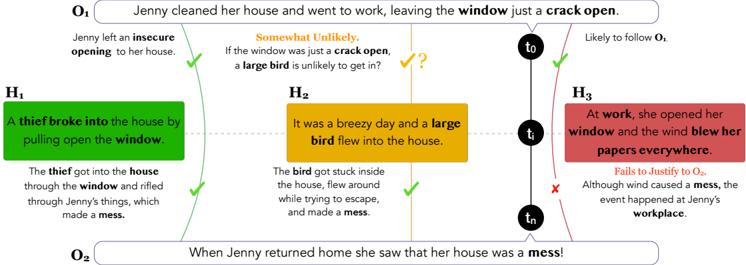- Jerry Hobbs, ACL 2013 Lifetime Achievement Award 1 Abductive reasoning is inference to the most plausible explanation for incomplete observations (Peirce, 1965a). Figure 1 illustrates an example. Given the incomplete observations about the world that O 1 : 'Jenny cleaned her house and went to work, leaving the window just a crack open.' and sometime later O 2 : 'When Jenny returned home, she saw her house was a mess.', we can hypothesize different potential explanations and reason about which is the most likely. We can readily rule out H 3 since it fails to justify the observation O 2 . While H 1 and H 2 are both plausible, the most likely explanation based on commonsense is H 1 as H 2 is somewhat implausible given O 1 . One crucial observation Peirce makes about abductive reasoning is that abduction is 'the only logical operation which introduces any new ideas' , which contrasts with other types of inference such as entailment, that focuses on inferring only such information that is already provided in the premise. ∗ Work done while at AI2 1 The full transcript of his award speech is available at https://www.mitpressjournals.org/ doi/full/10.1162/COLI\_a\_00171 Figure 1: Example of Abductive Reasoning. Given observations O 1 and O 2 , the α NLI task is to select the most plausible explanatory hypothesis. Since the number of hypotheses is massive in any given situation, we make a simplifying assumption in our ART dataset to only choose between a pair of explanations. <details> <summary>Image 1 Details</summary>  ### Visual Description ## Flowchart: Hypotheses for Jenny's Messy House ### Overview The flowchart illustrates three competing hypotheses (H1, H2, H3) explaining why Jenny's house was a mess when she returned home. It uses color-coded boxes, directional arrows, and symbolic markers (✓, ✗, ?) to represent causal relationships, likelihood assessments, and logical validity. The narrative spans three time points: t₀ (initial observation), tᵢ (intermediate event), and tₙ (final conclusion). --- ### Components/Axes - **Hypotheses (H1-H3)**: Three colored boxes (green, yellow, red) representing distinct scenarios. - **Outcomes (O1, O2)**: Two text nodes describing the initial and final states of the house. - **Timeline Markers**: t₀ (top), tᵢ (middle), tₙ (bottom) anchoring the narrative flow. - **Legend**: - Green ✓ = Likely causal link - Yellow ? = Uncertainty - Red ✗ = Invalid causal link - Orange = Neutral/transitional state --- ### Detailed Analysis #### Hypothesis H1 (Green) - **Label**: "A thief broke into the house by pulling open the window." - **Supporting Text**: - "The thief got into the house through the window and rifled through Jenny’s things, which made a mess." - **Connections**: - Direct arrow from O₁ (initial observation) with ✓ (likely). - Arrow to O₂ (final conclusion) with ✓ (likely). #### Hypothesis H2 (Yellow) - **Label**: "It was a breezy day and a large bird flew into the house." - **Supporting Text**: - "The bird got stuck inside the house, flew around while trying to escape, and made a mess." - **Connections**: - Arrow from O₁ with ✓ (likely). - Arrow to O₂ with ✓ (likely). - Intermediate question mark (?) questioning plausibility of a "large bird" entering through a "crack open" window. #### Hypothesis H3 (Red) - **Label**: "At work, she opened her window and the wind blew her papers everywhere." - **Supporting Text**: - "Fails to justify O₂. Although wind caused a mess, the event happened at Jenny’s workplace." - **Connections**: - Arrow from tᵢ to O₂ with ✗ (invalid). - Red color indicates logical inconsistency with O₂. --- ### Key Observations 1. **H1 and H2** are both marked as likely (✓) to explain O₂, but H1 is spatially prioritized (leftmost). 2. **H3** is explicitly rejected (✗) due to temporal mismatch (workplace vs. home). 3. **O1** serves as the premise for all hypotheses, while **O2** is the conclusion. 4. **tᵢ** acts as a pivot point separating H1/H2 (home-based causes) from H3 (workplace cause). --- ### Interpretation The flowchart demonstrates abductive reasoning, where multiple hypotheses are tested against observed outcomes. H1 and H2 are plausible explanations for the mess, but H3 is dismissed because its causal mechanism (wind at work) cannot account for the state of Jenny’s *home*. The use of color and symbols creates a visual hierarchy: green (valid) hypotheses dominate, while red (invalid) hypotheses are marginalized. The question mark in H2 introduces uncertainty about the plausibility of a "large bird" entering through a small opening, suggesting potential gaps in the narrative. The timeline anchors the story in chronological order, emphasizing that the mess occurred *after* Jenny left for work (t₀) and before her return (tₙ). </details> Abductive reasoning has long been considered to be at the core of understanding narratives (Hobbs et al., 1988), reading between the lines (Norvig, 1987; Charniak & Shimony, 1990), reasoning about everyday situations (Peirce, 1965b; Andersen, 1973), and counterfactual reasoning (Pearl, 2002; Pearl & Mackenzie, 2018). Despite the broad recognition of its importance, however, the study of abductive reasoning in narrative text has very rarely appeared in the NLP literature, in large part because most previous work on abductive reasoning has focused on formal logic, which has proven to be too rigid to generalize to the full complexity of natural language. In this paper, we present the first study to investigate the viability of language-based abductive reasoning. This shift from logic -based to language -based reasoning draws inspirations from a significant body of work on language-based entailment (Bowman et al., 2015; Williams et al., 2018b), language-based logic (Lakoff, 1970; MacCartney & Manning, 2007), and language-based commonsense reasoning (Mostafazadeh et al., 2016; Zellers et al., 2018). In particular, we investigate the use of natural language as the representation medium, and probe deep neural models on language-based abductive reasoning. More concretely, we propose Abductive Natural Language Inference ( α NLI) and Abductive Natural Language Generation ( α NLG) as two novel reasoning tasks in narrative contexts. 2 We formulate α NLI as a multiple-choice task to support easy and reliable automatic evaluation: given a context, the task is to choose the more likely explanation from a given pair of hypotheses choices. We also introduce a new challenge dataset, ART , that consists of 20K narratives accompanied by over 200K explanatory hypothesis. 34 We then establish comprehensive baseline performance based on state-of-the-art NLI and language models. The best baseline for α NLI based on BERT achieves 68.9% accuracy, with a considerable gap compared to human performance of 91.4%( § 5.2). The best generative model, based on GPT2, performs well below human performance on the α NLG task ( § 5.2). Our analysis leads to insights into the types of reasoning that deep pre-trained language models fail to perform - despite their strong performance on the closely related but different task of entailment NLI - pointing to future research directions. ## 2 TASK DEFINITION Abductive Natural Language Inference We formulate α NLI as multiple choice problems consisting of a pair of observations as context and a pair of hypothesis choices. Each instance in ART is defined as follows: - O 1 : The observation at time t 1 . 2 α NLI and α NLG are pronounced as alpha -NLI and alpha -NLG, respectively 3 ART : A bductive R easoning in narrative T ext. 4 Data available to download at http://abductivecommonsense.xyz - O 2 : The observation at time t 2 > t 1 . - h + : A plausible hypothesis that explains the two observations O 1 and O 2 . - h -: An implausible (or less plausible) hypothesis for observations O 1 and O 2 . Given the observations and a pair of hypotheses, the α NLI task is to select the most plausible explanation (hypothesis). Abductive Natural Language Generation α NLG is the task of generating a valid hypothesis h + given the two observations O 1 and O 2 . Formally, the task requires to maximize P ( h + | O 1 , O 2 ) . ## 3 MODELS FOR ABDUCTIVE COMMONSENSE REASONING ## 3.1 ABDUCTIVE NATURAL LANGUAGE INFERENCE A Probabilistic Framework for α NLI: A distinct feature of the α NLI task is that it requires jointly considering all available observations and their commonsense implications, to identify the correct hypothesis. Formally, the α NLI task is to select the hypothesis h ∗ that is most probable given the observations. 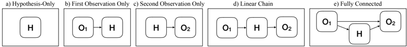$$h ^ { * } = \arg \max _ { h ^ { i } } P ( H = h ^ { i } | O _ { 1 } , O _ { 2 } ) \quad ( 1 )$$ Rewriting the objective using Bayes Rule conditioned on O 1 , we have: $$P ( h ^ { i } | O _ { 1 } , O _ { 2 } ) \varpropto P ( O _ { 2 } | h ^ { i } , O _ { 1 } ) P ( h ^ { i } | O _ { 1 } ) & & ( 2 )$$ We formulate a set of probabilistic models for α NLI that make various independence assumptions on Equation 2 - starting from a simple baseline that ignores the observations entirely, and building up to a fully joint model. These models are depicted as Bayesian Networks in Figure 2. Figure 2: Illustration of the graphical models described in the probabilistic framework. The 'Fully Connected' model can, in theory, combine information from both available observations. <details> <summary>Image 2 Details</summary>  ### Visual Description ## Diagram: Hypothesis-Observation Configurations ### Overview The image presents five distinct diagrams (a–e) illustrating different configurations of relationships between a central hypothesis node (H) and observation nodes (O₁, O₂). Each diagram represents a unique structural relationship, with directional arrows indicating dependencies or influences. ### Components/Axes - **Nodes**: - **H**: Central hypothesis node (appears in all diagrams). - **O₁/O₂**: Observation nodes (appear in diagrams b–e). - **Arrows**: Represent directional relationships (e.g., influence, dependency). - **Labels**: - Diagram titles (a–e) specify the configuration type. - Node labels (H, O₁, O₂) are consistent across diagrams. ### Detailed Analysis #### Diagram a) Hypothesis-Only - **Structure**: Single node labeled **H**. - **Interpretation**: Represents a hypothesis in isolation, with no observational data. #### Diagram b) First Observation Only - **Structure**: **O₁** → **H** (arrow from O₁ to H). - **Interpretation**: Observational data (O₁) influences or informs the hypothesis (H). #### Diagram c) Second Observation Only - **Structure**: **H** → **O₂** (arrow from H to O₂). - **Interpretation**: Hypothesis (H) predicts or generates observational data (O₂). #### Diagram d) Linear Chain - **Structure**: **O₁** → **H** → **O₂** (sequential dependency). - **Interpretation**: Observational data (O₁) informs the hypothesis (H), which in turn predicts a second observation (O₂). #### Diagram e) Fully Connected - **Structure**: **O₁** ↔ **H** ↔ **O₂** (bidirectional arrows between all nodes). - **Interpretation**: Hypothesis (H) and observations (O₁, O₂) mutually influence each other in a feedback loop. ### Key Observations 1. **Directionality**: Arrows in diagrams b–d indicate unidirectional influence, while diagram e shows bidirectional relationships. 2. **Node Presence**: - H is present in all diagrams. - O₁ appears in b, d, e; O₂ appears in c, d, e. 3. **Complexity**: Diagram e introduces the highest complexity with reciprocal relationships. ### Interpretation The diagrams collectively model how hypotheses and observations interact in scientific or analytical frameworks: - **Isolation (a)**: Hypothesis without empirical grounding. - **Unidirectional Influence (b, c, d)**: Observations either inform hypotheses (b, d) or are predicted by them (c, d). - **Feedback (e)**: Mutual reinforcement between hypothesis and observations, suggesting an iterative, self-correcting process. This progression from isolation to interconnectedness highlights the importance of bidirectional validation in robust hypothesis testing. Diagram e’s fully connected structure implies a dynamic system where hypotheses and observations co-evolve, aligning with principles of Bayesian inference or systems theory. </details> Hypothesis Only: Our simplest model makes the strong assumption that the hypothesis is entirely independent of both observations, i.e. ( H ⊥ O 1 , O 2 ) , in which case we simply aim to maximize the marginal P ( H ) . First (or Second) Observation Only: Our next two models make weaker assumptions: that the hypothesis depends on only one of the first O 1 or second O 2 observation. Linear Chain: Our next model uses both observations, but considers each observation's influence on the hypothesis independently , i.e. it does not combine information across the observations. Formally, the model assumes that the three variables 〈 O 1 , H, O 2 〉 form a linear Markov chain, where the second observation is conditionally independent of the first, given the hypothesis (i.e. ( O 1 ⊥ O 2 | H ) ). Under this assumption, we aim to maximize a somewhat simpler objective than Equation 2: $$h ^ { * } = \arg \max _ { h ^ { i } } P ( O _ { 2 } | h ^ { i } ) P ( h ^ { i } | O _ { 1 } ) w h e r e \left ( O _ { 1 } \perp O _ { 2 } | H \right ) \quad ( 3 )$$ Fully Connected: Finally, our most sophisticated model jointly models all three random variables as in Equation 2, and can in principle combine information across both observations to choose the correct hypothesis. 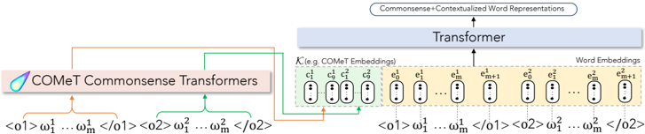Figure 3: Overview of an α NLG model that integrates commonsense representations obtained from COMeT(Bosselut et al., 2019) with GPT2. Each observation is input to the COMeT model to obtain nine embeddings, each associated with one commonsense inference type. <details> <summary>Image 3 Details</summary>  ### Visual Description ## Diagram: COMeT Commonsense Transformers Architecture ### Overview The diagram illustrates a technical architecture for generating **Commonsense+Contextualized Word Representations** using COMeT (Conceptual Commonsense Transformers). It depicts a multi-stage pipeline involving two COMeT Commonsense Transformers, a central Transformer, and word embedding outputs. The flow of data is represented through color-coded arrows (orange, green, blue) connecting components. --- ### Components/Axes 1. **COMeT Commonsense Transformers** - **Inputs**: - `<o1>` with parameters `ω₁ ... ωₘ` - `<o2>` with parameters `ω₁ ... ωₘ` - **Outputs**: - `c₁, c₉, c₁, c₉` (labeled as "COMeT Embeddings") 2. **Transformer** - **Inputs**: - `e₀, e₁, ..., eₘ, eₘ₊₁` (word embeddings) - **Outputs**: - `e₀, e₁, ..., eₘ, eₘ₊₁` (contextualized word embeddings) 3. **Word Embeddings** - Final output: `e₀, e₁, ..., eₘ, eₘ₊₁` **Legend**: - **Orange arrows**: Data flow from COMeT Transformers to the central Transformer. - **Green arrows**: Internal connections between COMeT outputs. - **Blue arrows**: Data flow from the Transformer to word embeddings. --- ### Detailed Analysis - **COMeT Transformers**: - Processes two input sequences (`<o1>` and `<o2>`) with shared parameter sets (`ω₁ ... ωₘ`). - Generates embeddings `c₁, c₉` (possibly representing concept or contextual features). - **Transformer**: - Integrates COMeT embeddings (`c₁, c₉`) with word embeddings (`e₀ ... eₘ₊₁`). - Produces contextualized word representations (`e₀ ... eₘ₊₁`). - **Embedding Flow**: - Inputs `<o1>` and `<o2>` are processed independently by COMeT, then merged via green arrows. - The merged output feeds into the Transformer, which refines embeddings through self-attention mechanisms. --- ### Key Observations 1. **Parameter Sharing**: - Both `<o1>` and `<o2>` share identical parameter sets (`ω₁ ... ωₘ`), suggesting a unified processing mechanism for different inputs. 2. **Embedding Hierarchy**: - COMeT embeddings (`c₁, c₉`) are distinct from word embeddings (`e₀ ... eₘ₊₁`), indicating a two-stage representation learning process. 3. **Contextualization**: - The final `e₀ ... eₘ₊₁` embeddings are enriched by the Transformer, implying dynamic context integration. --- ### Interpretation This architecture demonstrates a **multi-modal approach** to generating contextualized word representations: - **COMeT Transformers** extract commonsense knowledge from structured inputs (`<o1>`, `<o2>`). - The **central Transformer** combines these with lexical embeddings (`e₀ ... eₘ₊₁`) to produce context-aware representations. - The use of shared parameters (`ω₁ ... ωₘ`) suggests efficiency, while the two-stage process (COMeT + Transformer) balances domain-specific knowledge with general language understanding. **Notable Design Choices**: - The `c₁, c₉` embeddings may represent specific commonsense concepts (e.g., causality, hierarchy). - The `eₘ₊₁` output suggests the model handles variable-length sequences, common in transformer-based architectures. This design aligns with modern NLP pipelines that integrate symbolic knowledge (COMeT) with neural contextualization (Transformer) for robust language understanding. </details> To help illustrate the subtle distinction between how the Linear Chain and Fully Connected models consider both observations, consider the following example. Let observation O 1 : 'Carl went to the store desperately searching for flour tortillas for a recipe.' and O 2 : 'Carl left the store very frustrated.'. Then consider two distinct hypotheses, an incorrect h 1 : 'The cashier was rude' and the correct h 2 : 'The store had corn tortillas, but not flour ones.'. For this example, a Linear Chain model could arrive at the wrong answer, because it reasons about the observations separately-taking O 1 in isolation, both h 1 and h 2 seem plausible next events, albeit each a priori unlikely. And for O 2 in isolation-i.e. in the absence of O 1 , as for a randomly drawn shopper-the h 1 explanation of a rude cashier seems a much more plausible explanation of Carl's frustration than are the details of the store's tortilla selection. Combining these two separate factors leads the Linear Chain to select h 1 as the more plausible explanation. It is only by reasoning about Carl's goal in O 1 jointly with his frustration in O 2 , as in the Fully Connected model, that we arrive at the correct answer h 2 as the more plausible explanation. In our experiments, we encode the different independence assumptions in the best performing neural network model. For the hypothesis-only and single observation models, we can enforce the independencies by simply restricting the inputs of the model to only the relevant variables. On the other hand, the Linear Chain model takes all three variables as input, but we restrict the form of the model to enforce the conditional independence. Specifically, we learn a discriminative classifier: $$P _ { L i n e a r C h a i n } ( h | O _ { 1 } , O _ { 2 } ) \, \infty \, e ^ { \phi ( O _ { 1 } , h ) + \phi ^ { \prime } ( h , O _ { 2 } ) }$$ where φ and φ ′ are neural networks that produce scalar values. ## 3.2 ABDUCTIVE NATURAL LANGUAGE GENERATION Given h + = { w h 1 . . . w h l } , O 1 = { w o 1 1 . . . w o 1 m } and O 2 = { w o 2 1 . . . w o 2 n } as sequences of tokens, the α NLG task can be modeled as P ( h + | O 1 , O 2 ) = ∏ P ( w h i | w h <i , w o 1 1 . . . w o 1 m , w o 2 1 . . . w o 2 n ) Optionally, the model can also be conditioned on background knowledge K . 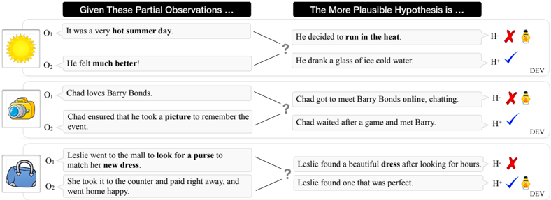Parameterized models can then be trained to minimize the negative log-likelihood over instances in ART : $$\mathcal { L } = - \sum _ { i = 1 } ^ { N } \log P ( w _ { i } ^ { h } | w _ { < i } ^ { h } , w _ { 1 } ^ { o 1 } \dots w _ { m } ^ { o 1 } , w _ { 1 } ^ { o 2 } \dots w _ { n } ^ { o 2 } , \mathcal { K } )$$ ## 4 ART DATASET: ABDUCTIVE REASONING IN NARRATIVE TEXT ART is the first large-scale benchmark dataset for studying abductive reasoning in narrative texts. It consists of ∼ 20K narrative contexts (pairs of observations 〈 O 1 , O 2 〉 ) with over 200K explanatory hypotheses. Table 6 in the Appendix summarizes corpus-level statistics of the ART dataset. 5 Figure 4 shows some illustrative examples from ART (dev split). The best model based on BERT fails to correctly predict the first two dev examples. 5 We will publicly release the ART dataset upon acceptance. Figure 4: Examples from ART (dev split). The best model based on BERT fails to correctly predict the first two examples. <details> <summary>Image 4 Details</summary>  ### Visual Description ## Flowchart: Hypothesis Evaluation Based on Observations ### Overview The image presents a flowchart with three scenarios, each containing partial observations (O1, O2) and two competing hypotheses (H⁻, H⁺). The hypotheses are evaluated for plausibility, with checkmarks (✓) and X marks indicating the more likely outcome. Visual icons (sun, camera, purse) accompany the observations. ### Components/Axes - **Main Structure**: - Three independent scenarios (top to bottom). - Each scenario includes: - **Observations**: Labeled O1 and O2 (textual descriptions). - **Hypotheses**: Labeled H⁻ (less plausible) and H⁺ (more plausible). - **Evaluation Symbols**: Red X (❌) for H⁻, blue checkmark (✓) for H⁺. - **Visual Elements**: - Icons: Sun (hot weather), camera (photography), purse (shopping). - Arrows connecting observations to hypotheses. - Question marks (?) linking observations to hypotheses. ### Detailed Analysis #### Scenario 1: Hot Summer Day - **Observations**: - O1: "It was a very hot summer day." (Icon: ☀️) - O2: "He felt much better!" - **Hypotheses**: - H⁻: "He decided to run in the heat." (❌) - H⁺: "He drank a glass of ice cold water." (✓) #### Scenario 2: Barry Bonds Fan - **Observations**: - O1: "Chad loves Barry Bonds." (Icon: 📸) - O2: "Chad ensured that he took a picture to remember the event." - **Hypotheses**: - H⁻: "Chad got to meet Barry Bonds online, chatting." (❌) - H⁺: "Chad waited after a game and met Barry." (✓) #### Scenario 3: Purses and Dresses - **Observations**: - O1: "Leslie went to the mall to look for a purse to match her new dress." (Icon: 👜) - O2: "She took it to the counter and paid right away, and went home happy." - **Hypotheses**: - H⁻: "Leslie found a beautiful dress after looking for hours." (❌) - H⁺: "Leslie found one that was perfect." (✓) ### Key Observations 1. **Consistency in Evaluation**: H⁺ (more plausible) is always marked with a checkmark (✓), while H⁻ is marked with an X (❌). 2. **Logical Alignment**: H⁺ hypotheses directly resolve the observations without contradiction (e.g., drinking water cools the body on a hot day). 3. **Visual Cues**: Icons reinforce the context of each observation (e.g., ☀️ for heat, 📸 for photography). ### Interpretation The flowchart demonstrates a framework for evaluating hypotheses based on observed facts. The checkmarks suggest that the most plausible hypothesis is the one that: - **Directly addresses the observations** (e.g., ice water alleviates heat discomfort). - **Avoids unnecessary assumptions** (e.g., meeting Barry Bonds online is less likely than meeting him in person after a game). - **Aligns with common-sense reasoning** (e.g., finding a "perfect" purse quickly implies satisfaction, unlike prolonged searching). This structure emphasizes the importance of grounding hypotheses in observable evidence and logical consistency, a principle applicable to scientific inquiry, problem-solving, and decision-making. </details> Collecting Observations: The pairs O 1 , O 2 in ART are drawn from the ROCStories dataset (Mostafazadeh et al., 2016). ROCStories is a large collection of short, manually curated fivesentence stories. It was designed to have a clear beginning and ending for each story, which naturally map to the first ( O 1 ) and second ( O 2 ) observations in ART . Collecting Hypotheses Options: We crowdsourced the plausible and implausible hypotheses options on Amazon Mechanical Turk (AMT) in two separate tasks 6 : 1. Plausible Hypothesis Options: We presented O 1 and O 2 as narrative context to crowdworkers who were prompted to fill in 'What happened in-between?' in natural language. The design of the task motivates the use of abductive reasoning to hypothesize likely explanations for the two given observations. 2. Implausible Hypothesis Options: In this task, we presented workers with observations O 1 , O 2 and one plausible hypothesis option h + ∈ H + collected from the previous task. Crowdworkers were instructed to make minimal edits (up to 5 words) to a given h + to create implausible hypothesis variations for each plausible hypothesis. A significant challenge in creating datasets is avoiding annotation artifacts - unintentional patterns in the data that leak information about the target label - that several recent studies (Gururangan et al., 2018; Poliak et al., 2018; Tsuchiya, 2018) have reported on crowdsourced datasets . To tackle this challenge, we collect multiple plausible and implausible hypotheses for each 〈 O 1 , O 2 〉 pair (as described above) and then apply an adversarial filtering algorithm to retain one challenging pair of hypotheses that are hard to distinguish between. We describe our algorithm in detail in Appendix A.5. While our final dataset uses BERT as the adversary, preliminary experiments that used GPT as an adversary resulted in similar drops in performance of all models, including all BERT variants. We compare the results of the two adversaries in Table 1. ## 5 EXPERIMENTS AND RESULTS We now present our evaluation of finetuned state-of-the-art pre-trained language models on the ART dataset, and several other baseline systems for both α NLI and α NLG. Since α NLI is framed as a binary classification problem, we choose accuracy as our primary metric. For α NLG, we report performance on automated metrics such as BLEU (Papineni et al., 2002), CIDEr (Vedantam et al., 2015), METEOR (Banerjee & Lavie, 2005) and also report human evaluation results. ## 5.1 ABDUCTIVE NATURAL LANGUAGE INFERENCE 6 Both crowdsourcing tasks are complex and require creative writing. Along with the ART dataset, we will publicly release templates and the full set of instructions for all crowdsourcing tasks to facilitate future data collection and research in this direction. Despite strong performance on several other NLP benchmark datasets, the best baseline model based on BERT achieves an accuracy of just 68.9% on ART compared to human performance of 91.4%. The large gap between human performance and that of the best system provides significant scope for development of more sophisticated abductive reasoning models. Our experiments show that introducing the additional independence assumptions described in Section 3.1 over the fully connected model tends to degrade system performance (see Table 1) in general. Human Performance We compute human performance using AMT. Each instance (two observations and two hypothesis choices) is shown to three workers who were prompted to choose the more plausible hypothesis choice. 7 We compute majority vote on the labels assigned which Table 1: Performance of baselines and finetuned-LM approaches on the test set of ART . Test accuracy is reported as the mean of five models trained with random seeds, with the standard deviation in parenthesis. | Model | GPT AF Acc. (%) | ART Acc. (%) | |----------------------------------|-------------------|----------------| | Random ( 2 -way choice) | 50.1 | 50.4 | | Majority (from dev set) | 50.1 | 50.8 | | Infersent (Conneau et al., 2017) | 50.9 | 50.8 | | ESIM+ELMo (Chen et al., 2017) | 58.2 | 58.8 | | Finetuning Pre-trained LMs | | | | GPT-ft | 52.6 (0.9) | 63.1 (0.5) | | BERT-ft [ h i Only] | 55.9 (0.7) | 59.5 (0.2) | | BERT-ft [ O 1 Only] | 63.9 (0.8) | 63.5 (0.7) | | BERT-ft [ O 2 Only] | 68.1 (0.6) | 66.6 (0.2) | | BERT-ft [Linear Chain] | 65.3 (1.4) | 68.9 (0.5) | | BERT-ft [Fully Connected] | 72.0 (0.5) | 68.6 (0.5) | | Human Performance | - | 91.4 | leads to a human accuracy of 91.4% on the ART test set. Baselines We include baselines that rely on simple features to verify that ART is not trivially solvable due to noticeable annotation artifacts, observed in several crowdsourced datasets. The accuracies of all simple baselines are close to chance-performance on the task - indicating that the dataset is free of simple annotation artifacts. A model for the related but distinct task of entailment NLI (e.g. SNLI) forms a natural baseline for α NLI. We re-train the ESIM+ELMo (Chen et al., 2017; Peters et al., 2018) model as its performance on entailment NLI ( 88 . 9% ) is close to state-of-the-art models (excluding pre-trained language models). This model only achieves an accuracy of 58 . 8% highlighting that performing well on ART requires models to go far beyond the linguistic notion of entailment. Pre-trained Language Models BERT (Devlin et al., 2018) and GPT (Radford, 2018) have recently been shown to achieve state-of-the-art results on several NLP benchmarks (Wang et al., 2018). We finetune both BERT-Large and GPT as suggested in previous work and we present each instance in their natural narrative order. BERT-ft (fully connected) is the best performing model achieving 68.9% accuracy, compared to GPT's 63 . 1% . 8 Our AF approach was able to reduce BERT performance from over 88% by 20 points. 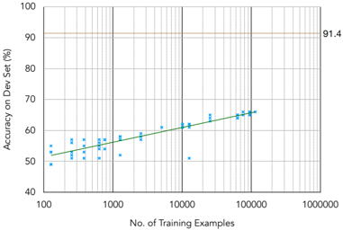Learning Curve and Dataset Size While there is enough scope for considerably scaling up the dataset based on ROCStories, the learning curve in Figure 5 shows that the performance of the best Figure 5: BERT learning curve on the dev set of ART . For each point on the x-axis, we fine-tune BERT with five random seeds. Human performance is 91.4%. <details> <summary>Image 5 Details</summary>  ### Visual Description ## Line Graph: Accuracy on Dev Set vs. Number of Training Examples ### Overview The image is a line graph depicting the relationship between the number of training examples and the accuracy of a model on a development set. The x-axis represents the number of training examples (ranging from 100 to 1,000,000), while the y-axis represents accuracy as a percentage (from 40% to 100%). A green trend line and blue data points illustrate the model's performance, with a red horizontal line marking a target accuracy of 91.4%. ### Components/Axes - **X-axis (Horizontal)**: "No. of Training Examples" (logarithmic scale: 100, 1,000, 10,000, 100,000, 1,000,000). - **Y-axis (Vertical)**: "Accuracy on Dev Set (%)" (linear scale: 40% to 100%). - **Legend**: - **Green line**: "Training Accuracy Trend" (solid line). - **Red line**: "Target Accuracy (91.4%)" (horizontal line at 91.4%). - **Data Points**: Blue "x" markers representing individual accuracy measurements at specific training example counts. ### Detailed Analysis - **Green Trend Line**: - Starts near **50%** at 100 training examples. - Increases gradually, reaching **~60%** at 10,000 examples. - Plateaus near **~65%** at 100,000 examples. - The line exhibits a logarithmic growth pattern, with diminishing returns as the number of examples increases. - **Blue Data Points**: - Scattered around the green trend line, with minor deviations (e.g., some points slightly below or above the line). - No significant outliers observed. - **Red Target Line**: - Horizontal line at **91.4%**, consistently above the green trend line across all training example counts. ### Key Observations 1. **Accuracy Growth**: The model's accuracy improves with more training data, but the rate of improvement slows significantly after 10,000 examples. 2. **Target Gap**: The model's accuracy (green line) remains **~26% below the target (91.4%)** even at 100,000 examples. 3. **Logarithmic Scaling**: The x-axis uses a logarithmic scale, emphasizing the exponential growth in training data required for incremental accuracy gains. ### Interpretation The graph demonstrates that increasing the number of training examples enhances model performance, but the improvement is not linear. The green trend line suggests diminishing returns, indicating that the model may be approaching a performance ceiling with the current architecture or data quality. The red target line (91.4%) highlights a critical gap, implying that either: - **More data** is needed to close the gap, or - **Model improvements** (e.g., architecture changes, hyperparameter tuning) are required to achieve the target accuracy. The logarithmic trend underscores the challenge of scaling machine learning models, where additional data yields smaller performance gains over time. This pattern is common in real-world scenarios, where data scarcity or model limitations constrain performance. </details> model plateaus after ∼ 10 , 000 instances. In addition, there is still a wide gap ( ∼ 23% ) between the performance of the best model and human performance. 7 Additional crowdsourcing details in the Appendix A.1 8 The input format for the GPT model and BERT variants is described in the Appendix A.4. Table 2: Performance of generative models on the test set of ART . All models except GPT2-Fixed are finetuned on ART . | Model | BLEU | METEOR | ROUGE | CIDEr | BERT-Score | Human | |--------------------------|--------|----------|---------|---------|--------------|---------| | GPT2-Fixed | 0 | 9.29 | 9.99 | 3.34 | 36.69 | - | | O 1 - O 2 - Only | 2.23 | 16.71 | 22.83 | 33.54 | 48.74 | 42.26 | | COMeT-Txt+GPT2 | 2.29 | 16.73 | 22.51 | 31.99 | 48.46 | 38.28 | | COMeT-Emb+GPT2 | 3.03 | 17.66 | 22.93 | 32 | 48.52 | 44.56 | | Human-written Hypotheses | 8.25 | 26.71 | 30.4 | 53.56 | 53.3 | 96.03 | GPT Adversary Table 1 also includes results of our experiments where GPT was used as the adversary. Notably, in this case, adversarially filtering the dataset brings down GPT performance under 53%. On the other hand, the best BERT model, that encodes the fully connected bayesian network performs significantly better than the BERT model that encodes the linear chain assumptions - 72% compared to 65%. Therefore, we use the BERT fully connected model as the adversary in ART . The gap between the linear chain and fully connected BERT models diminishes when BERT is used as an adversary - in spite of being a more powerful model - which indicates that adversarial filtering disproportionately impacts the model used as the adversary. However, the dataset also becomes more difficult for the other models that were not used as adversaries. For example, before any filtering, BERT scores 88% and OpenGPT gets 80% , which is much higher than either model achieves in Table 1 when the other model is used for filtering. This result is a reasonable indicator, albeit not a guarantee, that ART will remain challenging for new models released in the future. ## 5.2 ABDUCTIVE NATURAL LANGUAGE GENERATION Generative Language Models As described in Equation 4, we train GPT2 conditioned on the tokens of the two observations O 1 and O 2 . Both observations are enclosed with field-specific tags. ATOMIC (Sap et al., 2019), a repository of inferential if-then knowledge is a natural source of background commonsense required to reason about narrative contexts in ART . Yet, there is no straightforward way to include such knowledge into a neural model as ATOMIC's nodes are not canonicalized and are represented as short phrases of text. Thus, we rely on COMeT - a transformer model trained on ATOMIC that generates nine commonsense inferences of events in natural language. 9 Specifically, we experiment with two ways of integrating information from COMeT in GPT2: (i) as textual phrases , and (ii) as embeddings . Figure 3 shows how we integrate COMeT representations. Concretely, after the input tokens are embedded by the word-embedding layer, we append eighteen (corresponding to nine relations for each observation) embeddings to the sequence before passing through the layers of the Transformer architecture. This allows the model to learn each token's representation while attending to the COMeT embeddings - effectively integrating background commonsense knowledge into a language model. 10 Discussion Table 2 reports results on the α NLGtask. Among automatic metrics, we report BLEU4 (Papineni et al., 2002), METEOR (Banerjee & Lavie, 2005), ROUGE (Lin, 2004), CIDEr (Vedantam et al., 2015) and BERT-Score (Zhang et al., 2019) (with the bert-base-uncased model). We establish human performance through crowdsourcing on AMT. Crowdworkers are shown pairs of observations and a generated hypothesis and asked to label whether the hypothesis explains the given observations. The last column reports the human evaluation score. The last row reports the score of a held-out human-written hypothesis and serves as a ceiling for model performance. Human-written hypotheses are found to be correct for 96% of instances, while our best generative models, even when enhanced with background commonsense knowledge, only achieve 45% indicating that the α NLG generation task is especially challenging for current state-of-the-art text generators. 9 Please see Appendix A.6 for a full list of the nine relations. 10 We describe the format of input for each model in Appendix A.7. ## 6 ANALYSIS ## 6.1 α NLI Commonsense reasoning categories We investigate the categories of commonsense-based abductive reasoning that are challenging for current systems and the ones where the best model over-performs. While there have been previous attempts to categorize commonsense knowledge required for entailment (LoBue & Yates, 2011; Clark et al., 2007), crowdsourcing this task at scale with high fidelity and high agreement across annotators remains challenging. Instead, we aim to probe the model with soft categories identified by matching lists of category-specific keywords to the hypothesis choices. | Category | Human Accuracy | BERT Accuracy | ∆ | |------------------|------------------|-----------------|------| | All ( 1 , 000 ) | 91.4 | 68.8 | 22.6 | | Numerical ( 44 ) | 88.6 | 56.8 | 21.8 | | Spatial ( 130 ) | 91.5 | 65.4 | 26.1 | | Emotional ( 84 ) | 86.9 | 72.6 | 14.3 | Table 3: BERT's performance and human evaluation on categories for 1,000 instances from the test set, based on commonsense reasoning domains (Numerical, Spatial, Emotional). The number in parenthesis indicates the size of the category. Table 3 shows the accuracy of the best model (BERT-ft) across various categories of commonsense knowledge. BERT-ft significantly underperforms on instances involving Numerical ( 56 . 8% ) and Spatial ( 65 . 4% ) commonsense. These two categories include reasoning about numerical quantities and the spatial location of agents and objects, and highlight some of the limitations of the language models. In contrast, it significantly overperforms on the Emotional category ( 72 . 6% ) where the hypotheses exhibit strong textual cues about emotions and sentiments. Implausible transitions A model for an instance of the ART dataset should discard implausible hypotheses in the context of the two given observations. In narrative contexts, there are three main reasons for an implausible hypothesis to be labeled as such: 1. O 1 → h -: h -is unlikely to follow after the first observation O 1 . 2. h -→ O 2 : h -is plausible after O 1 but unlikely to precede the second observation O 2 . 3. Plausible: 〈 O 1 , h -, O 2 〉 is a coherent narrative and forms a plausible alternative, but it is less plausible than 〈 O 1 , h + , O 2 〉 . | Story Transition | %of Dataset | BERT-ft Fully Connected Acc. (%) | BERT-ft Linear Chain Acc. (%) | |-------------------------------|---------------|------------------------------------|---------------------------------| | O 1 → h - | 32.5 | 73.6 | 71.6 | | h - → O 2 | 45.3 | 69 | 70.5 | | Plausible | 22.2 | 62.5 | 58.5 | | All (1,000) | 100 | 69.1 | 68.2 | Table 4: Fraction of dataset for which a particular transition in the story is broken for the negative hypothesis, for 1,000 random instances from the test set. We analyze the prevalence of each of these reasons in ART . We design a crowdsourcing task in which we show the implausible option along with the narrative context 〈 O 1 , O 2 〉 and get labels for which transition ( O 1 → h -, h -→ O 2 or neither) in the narrative chain is broken. Table 4 shows the proportion of each category from a subset of 1 , 000 instances from the test set. While h -→ O 2 accounts for almost half of the implausible transitions in ART , all three categories are substantially present in the dataset. BERT performance on each of these categories indicates that the model finds it particularly hard when the narrative created by the incorrect hypothesis is plausible, but less plausible than the correct hypothesis. On that subset of the test set, the fully connected model performs better than the linear chain model where it is important to consider both observations jointly to arrive at the more likely hypothesis. 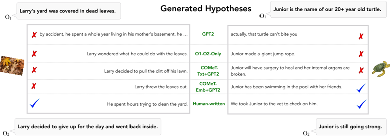## 6.2 α NLG Figure 6 shows some examples of generations from the trained models compared to human-written generations. The example on the left is an example of an instance that only humans could get correct, while for the one on the right, COMeT-Emb+GPT2 also generates the correct explanation for the observations. Figure 6: Examples of generated hypotheses from different models and human-written hypothesis for 2 instances from ART . <details> <summary>Image 6 Details</summary>  ### Visual Description ## Screenshot: Hypothesis Generation and Evaluation for Scenario O1 and O2 ### Overview The image compares generated hypotheses for two scenarios (O1 and O2) against actual outcomes. Each scenario includes hypotheses generated by different models (GPT2, COMeT-Txt+GPT2, COMeT-Emb+GPT2) and a human-written baseline. Correctness is marked with ✅ (correct) or ❌ (incorrect). The scenarios involve: - **O1**: Larry's yard covered in dead leaves. - **O2**: Junior, a 20+ year old turtle, is still going strong. ### Components/Axes - **Left Column (O1)**: - **Scenario**: "Larry’s yard was covered in dead leaves." - **Generated Hypotheses**: 1. **GPT2**: "By accident, he spent a whole year living in his mother’s basement, he …" ❌ 2. **O1-O2-Only**: "Larry wondered what he could do with the leaves." ❌ 3. **COMeT-Txt+GPT2**: "Larry decided to pull the dirt off his lawn." ❌ 4. **COMeT-Emb+GPT2**: "Larry threw the leaves out." ❌ 5. **Human-written**: "He spent hours trying to clean the yard." ✅ - **Actual Outcome**: "Larry decided to give up for the day and went back inside." ✅ (matches human-written hypothesis). - **Right Column (O2)**: - **Scenario**: "Junior is the name of our 20+ year old turtle." - **Generated Hypotheses**: 1. **GPT2**: "Actually, that turtle can’t bite you." ❌ 2. **O1-O2-Only**: "Junior made a giant jump rope." ❌ 3. **COMeT-Txt+GPT2**: "Junior will have surgery to heal and her internal organs are broken." ❌ 4. **COMeT-Emb+GPT2**: "Junior has been swimming in the pool with her friends." ✅ 5. **Human-written**: "We took Junior to the vet to check on him." ✅ - **Actual Outcome**: "Junior is still going strong." ✅ (matches both COMeT-Emb+GPT2 and human-written hypotheses). ### Detailed Analysis - **O1 Hypotheses**: - All model-generated hypotheses (GPT2, COMeT-Txt+GPT2, COMeT-Emb+GPT2) are incorrect. The human-written hypothesis aligns with the actual outcome. - Models generate implausible or unrelated narratives (e.g., living in a basement, throwing leaves out). - **O2 Hypotheses**: - **COMeT-Emb+GPT2** and **human-written** hypotheses are correct. The actual outcome ("Junior is still going strong") is directly supported by both. - Models produce mixed results: GPT2 and COMeT-Txt+GPT2 generate irrelevant or incorrect claims (e.g., "can’t bite you," "surgery to heal"). ### Key Observations 1. **Human-written hypotheses outperform models** in both scenarios, suggesting limitations in automated generation. 2. **COMeT-Emb+GPT2** shows partial success (correct for O2 but not O1), indicating model-specific strengths. 3. **O1-O2-Only** hypotheses are consistently incorrect, highlighting a lack of contextual understanding. 4. **GPT2** generates the most implausible hypotheses (e.g., "giant jump rope" for a turtle). ### Interpretation - **Model Limitations**: Automated systems struggle with contextual coherence, often producing irrelevant or factually incorrect hypotheses. This underscores the need for hybrid approaches combining model outputs with human validation. - **COMeT-Emb+GPT2’s Partial Success**: The model’s ability to generate correct hypotheses for O2 suggests that embedding (COMeT-Emb) may improve relevance for specific domains (e.g., animal care). - **Human Role**: Human-written hypotheses directly reflect real-world outcomes, emphasizing the irreplaceable value of human judgment in complex reasoning tasks. - **Scenario Dependency**: Model performance varies by context (e.g., O1 vs. O2), indicating the need for scenario-specific fine-tuning or prompt engineering. ### Technical Notes - **Color Coding**: Not applicable (text-based screenshot). - **Spatial Layout**: Two-column structure separates O1 (left) and O2 (right), with hypotheses listed vertically under each scenario. - **Text Extraction**: All labels, hypotheses, and outcomes are transcribed verbatim. No non-English text present. </details> ## 7 TRANSFER LEARNING FROM ART ART contains a large number of questions for the novel abductive reasoning task. In addition to serving as a benchmark, we investigate if ART can be used as a resource to boost performance on other commonsense tasks. We apply transfer learning by first training a model on ART , and subsequently training on four target datasets - WinoGrande Sakaguchi et al. (2020), WSC Levesque et al. (2011), DPR Rahman & Ng (2012) and HellaSwag Zellers et al. (2019). We show that compared to a model that is only trained on the target dataset, a model that is sequentially trained on ART first and then on the target dataset can perform better. In particular, pre-training on ART consistently improves performance on related datasets when they have relatively few training examples. On the other hand, for target datasets with large amounts of training data, pre-training on ART does not provide a significant improvement. ## 8 RELATED WORK Cloze-Style Task vs. Abductive Reasoning Since abduction is fundamentally concerned with plausible chains of cause-and-effect, our work draws inspiration from previous works that deal with narratives such as script learning Table 5: Transfer Learning from ART | Dataset | BERT-ft(D) | BERT-ft( ART ) → BERT-ft(D) | |----------------------------------------------|--------------|-------------------------------| | WinoGrande Sakaguchi et al. (2020) | 65.8% | 67.2 % | | WSC | 70.0% | 74.0 % | | Levesque et al. (2011) DPR Rahman &Ng (2012) | 72.5% | 86.0 % | | Hellaswag Zellers et al. (2019) | 46.7 % | 46.1% | (Schank & Abelson, 1975) and the narrative cloze test (Chambers & Jurafsky, 2009; Jans et al., 2012; Pichotta & Mooney, 2014; Rudinger et al., 2015). Rather than learning prototypical scripts or narrative chains, we instead reason about the most plausible events conditioned on observations. We make use of the ROCStories dataset (Mostafazadeh et al., 2016), which was specifically designed for the narrative cloze task. But, instead of reasoning about plausible event sequences, our task requires reasoning about plausible explanations for narrative omissions. Entailment vs. Abductive Reasoning The formulation of α NLI is closely related to entailment NLI, but there are two critical distinctions that make abductive reasoning uniquely challenging. First, abduction requires reasoning about commonsense implications of observations (e.g., if we observe that the 'grass is wet', a likely hypothesis is that 'it rained earlier') which go beyond the linguistic notion of entailment (also noted by Josephson (2000)). Second, abduction requires non-monotonic reasoning about a set of commonsense implications collectively, to check the potential contradictions against multiple observations and to compare the level of plausibility of different hypotheses. This makes abductive reasoning distinctly challenging compared to other forms of reasoning such as induction and deduction (Shank, 1998). Perhaps more importantly, abduction is closely related to the kind of reasoning humans perform in everyday situations, where information is incomplete and definite inferences cannot be made. Generative Language Modeling Recent advancements in the development of large-scale pretrained language models (Radford, 2018; Devlin et al., 2018; Radford et al., 2019) have improved the quality and coherence of generated language. Although these models have shown to generate reasonably coherent text when condition on a sequence of text, our experiments highlight the limitations of these models to 1) generate language non-monotonically and 2) adhere to commonsense knowledge. We attempt to overcome these limitations with the incorporation of a generative commonsense model during hypothesis generation. Related Datasets Our new resource ART complements ongoing efforts in building resources for natural language inference (Dagan et al., 2006; MacCartney & Manning, 2009; Bowman et al., 2015; Williams et al., 2018a; Camburu et al., 2018). Existing datasets have mostly focused on textual entailment in a deductive reasoning set-up (Bowman et al., 2015; Williams et al., 2018a) and making inferences about plausible events (Maslan et al., 2015; Zhang et al., 2017). In their typical setting, these datasets require a system to deduce the logically entailed consequences of a given premise . In contrast, the nature of abduction requires the use of commonsense reasoning capabilities, with less focus on lexical entailment. While abductive reasoning has been applied to entailment datasets (Raina et al., 2005), they have been applied in a logical theorem-proving framework as an intermediate step to perform textual entailment - a fundamentally different task than α NLI. ## 9 CONCLUSION We present the first study that investigates the viability of language-based abductive reasoning. We conceptualize and introduce Abductive Natural Language Inference ( α NLI) - a novel task focused on abductive reasoning in narrative contexts. The task is formulated as a multiple-choice questionanswering problem. We also introduce Abductive Natural Language Generation ( α NLG) - a novel task that requires machines to generate plausible hypotheses for given observations. To support these tasks, we create and introduce a new challenge dataset, ART , which consists of 20,000 commonsense narratives accompanied with over 200,000 explanatory hypotheses. In our experiments, we establish comprehensive baseline performance on this new task based on state-of-the-art NLI and language models, which leads to 68.9% accuracy with a considerable gap with human performance (91.4%). The α NLG task is significantly harder - while humans can write a valid explanation 96% of times, the best generator models can only achieve 45%. Our analysis leads to new insights into the types of reasoning that deep pre-trained language models fail to perform - despite their strong performance on the closely related but different task of entailment NLI - pointing to interesting avenues for future research. We hope that ART will serve as a challenging benchmark for future research in languagebased abductive reasoning and the α NLI and α NLG tasks will encourage representation learning that enables complex reasoning capabilities in AI systems. ## ACKNOWLEDGMENTS We thank the anonymous reviewers for their insightful feedback. This research was supported in part by NSF (IIS-1524371), the National Science Foundation Graduate Research Fellowship under Grant No. DGE 1256082, DARPA CwC through ARO (W911NF15-1- 0543), DARPA MCS program through NIWC Pacific (N66001-19-2-4031), and the Allen Institute for AI. Computations on beaker.org were supported in part by credits from Google Cloud. ## REFERENCES Henning Andersen. Abductive and deductive change. Language , pp. 765-793, 1973. URL https: //www.jstor.org/stable/pdf/412063.pdf . Satanjeev Banerjee and Alon Lavie. Meteor: An automatic metric for mt evaluation with improved correlation with human judgments. In Proceedings of the acl workshop on intrinsic and extrinsic evaluation measures for machine translation and/or summarization , pp. 65-72, 2005. - Antoine Bosselut, Hannah Rashkin, Maarten Sap, Chaitanya Malaviya, Asli Celikyilmaz, and Yejin Choi. Comet: Commonsense transformers for automatic knowledge graph construction. arXiv preprint arXiv:1906.05317 , 2019. - Samuel R. Bowman, Gabor Angeli, Christopher Potts, and Christopher D. Manning. A large annotated corpus for learning natural language inference. In Proceedings of the 2015 Conference on Empirical Methods in Natural Language Processing (EMNLP) . Association for Computational Linguistics, 2015. URL https://nlp.stanford.edu/pubs/snli\_paper.pdf . - Oana-Maria Camburu, Tim Rockt¨ aschel, Thomas Lukasiewicz, and Phil Blunsom. e-snli: Natural language inference with natural language explanations. In Advances in Neural Information Processing Systems , pp. 9560-9572, 2018. URL https://papers.nips.cc/paper/ 8163-e-snli-natural-language-inference-with-natural-language-explanations. pdf . - Nathanael Chambers and Dan Jurafsky. Unsupervised learning of narrative schemas and their participants. In Proceedings of the Joint Conference of the 47th Annual Meeting of the ACL and the 4th International Joint Conference on Natural Language Processing of the AFNLP , pp. 602-610, Suntec, Singapore, August 2009. Association for Computational Linguistics. URL http://www.aclweb.org/anthology/P/P09/P09-1068 . - Eugene Charniak and Solomon Eyal Shimony. Probabilistic semantics for cost based abduction . Brown University, Department of Computer Science, 1990. URL https://www.aaai.org/ Papers/AAAI/1990/AAAI90-016.pdf . - Qian Chen, Xiao-Dan Zhu, Zhen-Hua Ling, Si Wei, Hui Jiang, and Diana Inkpen. Enhanced lstm for natural language inference. In ACL , 2017. URL https://www.aclweb.org/anthology/ P17-1152 . - Peter E. Clark, Philip Harrison, John A. Thompson, William R. Murray, Jerry R. Hobbs, and Christiane Fellbaum. On the role of lexical and world knowledge in rte3. In ACL-PASCAL@ACL , 2007. URL https://www.aclweb.org/anthology/W07-1409 . - Alexis Conneau, Douwe Kiela, Holger Schwenk, Lo¨ ıc Barrault, and Antoine Bordes. Supervised learning of universal sentence representations from natural language inference data. In Proceedings of the 2017 Conference on Empirical Methods in Natural Language Processing , pp. 670680, Copenhagen, Denmark, September 2017. Association for Computational Linguistics. doi: 10.18653/v1/D17-1070. URL https://www.aclweb.org/anthology/D17-1070 . - Ido Dagan, Oren Glickman, and Bernardo Magnini. The pascal recognising textual entailment challenge. In Machine learning challenges. evaluating predictive uncertainty, visual object classification, and recognising tectual entailment , pp. 177-190. Springer, 2006. URL http: //u.cs.biu.ac.il/˜dagan/publications/RTEChallenge.pdf . - Jacob Devlin, Ming-Wei Chang, Kenton Lee, and Kristina Toutanova. Bert: Pre-training of deep bidirectional transformers for language understanding. arXiv preprint arXiv:1810.04805 , 2018. URL https://arxiv.org/abs/1810.04805 . - Suchin Gururangan, Swabha Swayamdipta, Omer Levy, Roy Schwartz, Samuel Bowman, and Noah A. Smith. Annotation artifacts in natural language inference data. In Proceedings of the 2018 Conference of the North American Chapter of the Association for Computational Linguistics: Human Language Technologies, Volume 2 (Short Papers) , pp. 107-112, New Orleans, Louisiana, June 2018. Association for Computational Linguistics. doi: 10.18653/v1/N18-2017. URL https://www.aclweb.org/anthology/N18-2017 . - Jerry R. Hobbs, Mark Stickel, Paul Martin, and Douglas Edwards. Interpretation as abduction. In Proceedings of the 26th Annual Meeting of the Association for Computational Linguistics , pp. 95-103, Buffalo, New York, USA, June 1988. Association for Computational Linguistics. doi: 10.3115/982023.982035. URL https://www.aclweb.org/anthology/P88-1012 . - Bram Jans, Steven Bethard, Ivan Vuli´ c, and Marie-Francine Moens. Skip n-grams and ranking functions for predicting script events. In Proceedings of the 13th Conference of the European Chapter of the Association for Computational Linguistics , pp. 336-344, Avignon, France, April 2012. Association for Computational Linguistics. URL http://www.aclweb.org/anthology/ E12-1034 . - Susan G. Josephson. Abductive inference: Computation , philosophy , technology. 2000. URL https://philpapers.org/rec/JOSAIC . - George Lakoff. Linguistics and natural logic. Synthese , 22(1-2):151-271, 1970. URL https: //link.springer.com/article/10.1007/BF00413602 . - Hector J. Levesque, Ernest Davis, and Leora Morgenstern. The winograd schema challenge. In KR , 2011. - Chin-Yew Lin. Rouge: A package for automatic evaluation of summaries. Text Summarization Branches Out , 2004. - Peter LoBue and Alexander Yates. Types of common-sense knowledge needed for recognizing textual entailment. In ACL , 2011. URL https://www.aclweb.org/anthology/ P11-2057 . - Bill MacCartney and Christopher D. Manning. Natural logic for textual inference. In Proceedings of the ACL-PASCAL Workshop on Textual Entailment and Paraphrasing , pp. 193-200, Prague, June 2007. Association for Computational Linguistics. URL https://www.aclweb.org/ anthology/W07-1431 . - Bill MacCartney and Christopher D. Manning. An extended model of natural logic. In Proceedings of the Eight International Conference on Computational Semantics , pp. 140-156, Tilburg, The Netherlands, January 2009. Association for Computational Linguistics. URL https://www. aclweb.org/anthology/W09-3714 . - Nicole Maslan, Melissa Roemmele, and Andrew S. Gordon. One hundred challenge problems for logical formalizations of commonsense psychology. In AAAI Spring Symposia , 2015. URL http://people.ict.usc.edu/˜gordon/publications/AAAI-SPRING15.PDF . - Nasrin Mostafazadeh, Nathanael Chambers, Xiaodong He, Devi Parikh, Dhruv Batra, Lucy Vanderwende, Pushmeet Kohli, and James Allen. A corpus and cloze evaluation for deeper understanding of commonsense stories. In Proceedings of the 2016 Conference of the North American Chapter of the Association for Computational Linguistics: Human Language Technologies (NAACL) , pp. 839-849. Association for Computational Linguistics, 2016. doi: 10.18653/v1/N16-1098. URL http://aclweb.org/anthology/N16-1098 . - Peter Norvig. Inference in text understanding. In AAAI , pp. 561-565, 1987. URL http:// norvig.com/aaai87.pdf . - Kishore Papineni, Salim Roukos, Todd Ward, and Wei-Jing Zhu. Bleu: a method for automatic evaluation of machine translation. In ACL , 2002. - Judea Pearl. Reasoning with cause and effect. AI Magazine , 23(1):95, 2002. URL https:// ftp.cs.ucla.edu/pub/stat\_ser/r265-ai-mag.pdf . - Judea Pearl and Dana Mackenzie. The Book of Why: The New Science of Cause and Effect . Basic Books, Inc., New York, NY, USA, 1st edition, 2018. ISBN 046509760X, 9780465097609. URL https://dl.acm.org/citation.cfm?id=3238230 . - Charles Sanders Peirce. Collected papers of Charles Sanders Peirce , volume 5. Harvard University Press, 1965a. URL http://www.hup.harvard.edu/catalog.php?isbn= 9780674138001 . - Charles Sanders Peirce. Pragmatism and pragmaticism , volume 5. Belknap Press of Harvard University Press, 1965b. URL https://www.jstor.org/stable/224970 . - Jeffrey Pennington, Richard Socher, and Christopher Manning. Glove: Global vectors for word representation. In Proceedings of the 2014 Conference on Empirical Methods in Natural Language Processing (EMNLP) , pp. 1532-1543, Doha, Qatar, October 2014. Association for Computational Linguistics. doi: 10.3115/v1/D14-1162. URL https://www.aclweb.org/anthology/ D14-1162 . - Matthew Peters, Mark Neumann, Mohit Iyyer, Matt Gardner, Christopher Clark, Kenton Lee, and Luke Zettlemoyer. Deep contextualized word representations. In Proceedings of the 2018 Conference of the North American Chapter of the Association for Computational Linguistics: Human Language Technologies, Volume 1 (Long Papers) , pp. 2227-2237, New Orleans, Louisiana, June 2018. Association for Computational Linguistics. doi: 10.18653/v1/N18-1202. URL https://www.aclweb.org/anthology/N18-1202 . - Karl Pichotta and Raymond Mooney. Statistical script learning with multi-argument events. In Proceedings of the 14th Conference of the European Chapter of the Association for Computational Linguistics , pp. 220-229, Gothenburg, Sweden, April 2014. Association for Computational Linguistics. URL http://www.aclweb.org/anthology/E14-1024 . - Adam Poliak, Jason Naradowsky, Aparajita Haldar, Rachel Rudinger, and Benjamin Van Durme. Hypothesis only baselines in natural language inference. In Proceedings of the Seventh Joint Conference on Lexical and Computational Semantics , pp. 180-191, New Orleans, Louisiana, June 2018. Association for Computational Linguistics. doi: 10.18653/v1/S18-2023. URL https: //www.aclweb.org/anthology/S18-2023 . - Alec Radford. Improving language understanding by generative pre-training. 2018. - Alec Radford, Jeffrey Wu, Rewon Child, David Luan, Dario Amodei, and Ilya Sutskever. Language models are unsupervised multitask learners. OpenAI Blog , 1(8), 2019. - Altaf Rahman and Vincent Ng. Resolving complex cases of definite pronouns: The winograd schema challenge. In EMNLP-CoNLL , 2012. - Rajat Raina, Andrew Y Ng, and Christopher D Manning. Robust textual inference via learning and abductive reasoning. In AAAI , pp. 1099-1105, 2005. URL https://nlp.stanford.edu/ ˜manning/papers/aaai05-learnabduction.pdf . - Rachel Rudinger, Pushpendre Rastogi, Francis Ferraro, and Benjamin Van Durme. Script induction as language modeling. In Proceedings of the 2015 Conference on Empirical Methods in Natural Language Processing , pp. 1681-1686, Lisbon, Portugal, September 2015. Association for Computational Linguistics. URL http://aclweb.org/anthology/D15-1195 . - Keisuke Sakaguchi, Ronan Le Bras, Chandra Bhagavatula, and Yejin Choi. Winogrande: An adversarial winograd schema challenge at scale. In AAAI , 2020. - Maarten Sap, Ronan Le Bras, Emily Allaway, Chandra Bhagavatula, Nicholas Lourie, Hannah Rashkin, Brendan Roof, Noah A Smith, and Yejin Choi. Atomic: an atlas of machine commonsense for if-then reasoning. In Proceedings of the AAAI Conference on Artificial Intelligence , volume 33, pp. 3027-3035, 2019. - Roger C. Schank and Robert P. Abelson. Scripts, plans, and knowledge. In Proceedings of the 4th International Joint Conference on Artificial Intelligence - Volume 1 , IJCAI'75, pp. 151-157, San Francisco, CA, USA, 1975. Morgan Kaufmann Publishers Inc. URL http://dl.acm.org/ citation.cfm?id=1624626.1624649 . - Gary Shank. The extraordinary ordinary powers of abductive reasoning. Theory & Psychology , 8(6):841-860, 1998. URL https://journals.sagepub.com/doi/10.1177/ 0959354398086007 . - Masatoshi Tsuchiya. Performance impact caused by hidden bias of training data for recognizing textual entailment. CoRR , abs/1804.08117, 2018. URL http://www.lrec-conf.org/ proceedings/lrec2018/pdf/786.pdf . - Ramakrishna Vedantam, C Lawrence Zitnick, and Devi Parikh. Cider: Consensus-based image description evaluation. In Proceedings of the IEEE conference on computer vision and pattern recognition , pp. 4566-4575, 2015. - Alex Wang, Amanpreet Singh, Julian Michael, Felix Hill, Omer Levy, and Samuel Bowman. GLUE: A multi-task benchmark and analysis platform for natural language understanding. In Proceedings of the 2018 EMNLP Workshop BlackboxNLP: Analyzing and Interpreting Neural Networks for NLP , pp. 353-355, Brussels, Belgium, November 2018. Association for Computational Linguistics. URL https://www.aclweb.org/anthology/W18-5446 . - Adina Williams, Nikita Nangia, and Samuel Bowman. A broad-coverage challenge corpus for sentence understanding through inference. In Proceedings of the 2018 Conference of the North American Chapter of the Association for Computational Linguistics: Human Language Technologies, Volume 1 (Long Papers) , pp. 1112-1122. Association for Computational Linguistics, 2018a. URL http://aclweb.org/anthology/N18-1101 . - Adina Williams, Nikita Nangia, and Samuel Bowman. A broad-coverage challenge corpus for sentence understanding through inference. In Proceedings of the 2018 Conference of the North American Chapter of the Association for Computational Linguistics: Human Language Technologies, Volume 1 (Long Papers) , pp. 1112-1122, New Orleans, Louisiana, June 2018b. Association for Computational Linguistics. doi: 10.18653/v1/N18-1101. URL https://www.aclweb. org/anthology/N18-1101 . - Rowan Zellers, Yonatan Bisk, Roy Schwartz, and Yejin Choi. Swag: A large-scale adversarial dataset for grounded commonsense inference. In Proceedings of the 2018 Conference on Empirical Methods in Natural Language Processing (EMNLP) , 2018. URL https://aclweb. org/anthology/D18-1009 . - Rowan Zellers, Ari Holtzman, Yonatan Bisk, Ali Farhadi, and Yejin Choi. Hellaswag: Can a machine really finish your sentence? In ACL , 2019. - Sheng Zhang, Rachel Rudinger, Kevin Duh, and Benjamin Van Durme. Ordinal common-sense inference. Transactions of the Association for Computational Linguistics , 5:379-395, 2017. doi: 10.1162/tacl a 00068. URL https://www.aclweb.org/anthology/Q17-1027 . - Tianyi Zhang, Varsha Kishore, Felix Wu, Kilian Q Weinberger, and Yoav Artzi. Bertscore: Evaluating text generation with bert. arXiv preprint arXiv:1904.09675 , 2019. ## A APPENDICES ## A.1 DATA COLLECTION DETAILS We describe the crowdsourcing details of our data collection method. Task 1 - Plausible Hypothesis Options In this task, participants were presented an incomplete three-part story, which consisted of the first observation ( O 1 ) and the second observation ( O 2 ) of the story. They were then asked to complete the story by writing a probable middle sentence that explains why the second observation should follow after the first one. We instructed participants to make sure that the plausible middle sentence (1) is short (fewer than 10 words) and (2) simple as if narrating to a child, (3) avoids introducing any extraneous information, and (4) uses names instead of pronouns (e.g., he/she) wherever possible. All participants were required to meet the following qualification requirements: (1) their location is in the US, (2) HIT approval rate is greater than 95(%), and (3) Number of HITs approved is greater than 5,000. The reward of this task was set to be $0.07 per question ($14/hour in average), and each HIT was assigned to five different workers (i.e., 5-way redundancy). Task 2 - Implausible Hypothesis Options In this task, participants were presented a three-part story, which consisted of the first observation ( O 1 ), a middle sentence ( h + ) collected in Task 1, and the second observation ( O 2 ) of the story. They were then asked to rewrite the middle sentence ( h + ) with minimal changes , so that the story becomes unlikely, implausible or inconsistent ( h -). We asked participants to add or remove at most four words to h + , while ensuring that the new middle sentence is grammatical. In addition, we asked them to stick to the context in the given story. For example, if the story talks about 'doctors', they are welcome to talk about 'health' or 'diagnosis', but not mention 'aliens'. Finally, we also asked workers to verify if the given middle ( h + ) makes a plausible story, in order to confirm the plausibility of h + collected in Task 1. With respect to this task's qualification, participants were required to fulfill the following requirements: (1) their location is the US or Canada, (2) HIT approval rate is greater than or equal to 99(%), and (3) number of HITs approved is greater than or equal to 10 , 000 . Participants were paid $0.1 per question ($14/hour in average), and each HIT was assigned to three different participants (i.e., 3-way redundancy). Task 3 α NLI Human Performance Human performance was evaluated by asking participants to answer the α NLI questions. Given a narrative context 〈 O 1 , O 2 〉 and two hypotheses, they were asked to choose the more plausible hypothesis. They were also allowed to choose 'None of the above' when neither hypothesis was deemed plausible. We asked each question to seven participants with the following qualification requirements: (1) their location is either in the US, UK, or Canada, (2) HIT approval rate is greater than 98(%), (3) Number of HITs approved is greater than 10 , 000 . The reward was set to $0.05 per HIT. We took the majority vote among the seven participants for every question to compute human performance. ## A.2 ART DATA STATISTICS Table 6 shows some statistics of the ART dataset. ## A.3 FINE-TUNING BERT We fine-tuned the BERT model using a grid search with the following set of hyper-parameters: - batch size: { 3 , 4 , 8 } - number of epochs: { 3 , 4 , 10 } - learning rate: { 1e-5, 2e-5, 3e-5, 5e-5 } The warmup proportion was set to 0 . 2 , and cross-entropy was used for computing the loss. The best performance was obtained with a batch size of 4 , learning rate of 5e-5, and number of epochs equal to 10 . Table 7 describes the input format for GPT and BERT (and its variants). | | Train | Dev | Test | |--------------------------|---------|-------|--------| | Total unique occurrences | | | | | Contexts 〈 O 1 , O 2 〉 | 17,801 | 1,532 | 3,059 | | Plausible hyp. h + | 72,046 | 1,532 | 3,059 | | Implausible hyp. h - | 166,820 | 1,532 | 3,059 | | Avg. size per context | | | | | Plausible hyp. h + | 4.05 | 1 | 1 | | Implausible hyp. h - | 9.37 | 1 | 1 | | Avg. word length | | | | | Plausible hyp. h + | 8.34 | 8.62 | 8.54 | | Implausible hyp. h - | 8.28 | 8.55 | 8.53 | | First observation O 1 | 8.09 | 8.07 | 8.17 | | Second observation O 2 | 9.29 | 9.3 | 9.31 | Table 6: Some statistics summarizing the ART dataset. The train set includes all plausible and implausible hypotheses collected via crowdsourcing, while the dev and test sets include the hypotheses selected through the Adversarial Filtering algorithm. ## A.4 BASELINES The SVM classifier is trained on simple features like word length, overlap and sentiment features to select one of the two hypothesis choices. The bag-of-words baseline computes the average of GloVe (Pennington et al., 2014) embeddings for words in each sentence to form sentence embeddings. The sentence embeddings in a story (two observations and a hypothesis option) are concatenated and passed through fully-connected layers to produce a score for each hypothesis. The accuracies of both baselines are close to 50% (SVM: 50.6; BOW: 50.5). Specifically, we train an SVM classifier and a bag-of-words model using GLoVE embeddings. Both models achieve accuracies close to 50%. An Infersent (Conneau et al., 2017) baseline that uses sentences embedded by max-pooling over Bi-LSTM token representations achieves only 50.8% accuracy. Table 7: Input formats for GPT and BERT fine-tuning. | Model | Input Format | Input Format | Input Format | Input Format | Input Format | Input Format | Input Format | Input Format | Input Format | Input Format | Input Format | Input Format | Input Format | |--------------------------------------------------------------------|----------------|----------------|----------------|----------------|----------------|----------------|----------------|----------------|----------------|----------------|----------------|----------------|----------------| | GPT | [START] | O 1 + | h i | [SEP] | | O | 2 | [SEP] | | | | | | | BERT-ft [Hypothesis Only] | [CLS] | h i | [SEP] | | | | | | | | | | | | BERT-ft [First Observation Only] BERT-ft [Second Observation Only] | [CLS] [CLS] | O 1 h i | [SEP] [SEP] | O | h i 2 | [SEP] | [SEP] | | | | O 2 | | | | BERT-ft [Linear Chain] | [CLS] | O 1 | [SEP] | | h i | [SEP] | ; | [CLS] | h i | [SEP] | | [SEP] | | | BERT-ft [Fully Connected] | [CLS] | O 1 | + O 2 | | [SEP] | h i | | [SEP] | | | | | | ## A.5 ADVERSARIAL FILTERING OF HYPOTHESES CHOICES Given an observation pair and sets of plausible and implausible hypotheses 〈 O 1 , O 2 , H + , H -〉 , our adversarial filtering algorithm selects one plausible and one implausible hypothesis 〈 O 1 , O 2 , h + , h -〉 such that h + and h -are hard to distinguish between. We make three key improvements over the previously proposed Adversarial Filtering (AF) approach in Zellers et al. (2018). First, Instead of a single positive sample, we exploit a pool H + of positive samples to choose from (i.e. plausible hypotheses). Second, Instead of machine generated distractors, the pool H -of negative samples (i.e. implausible hypotheses) is human-generated. Thus, the distractors share stylistic features of the positive samples as well as that of the context (i.e. observations O 1 and O 2 ) - making the negative samples harder to distinguish from positive samples. Finally, We use BERT (Devlin et al., 2018) as the adversary and introduce a temperature parameter that controls the maximum number of instances that can be modified in each iteration of AF. In later iterations, fewer instances get modified resulting in a smoother convergence of the AF algorithm (described in more detail below). Algorithm 1 provides a formal description of our approach. In each iteration i , we train an adversarial model M i on a random subset T i of the data and update the validation set V i to make it more challenging for M i . For a pair ( h + k , h -k ) of plausible and implausible hypotheses for an instance k , we denote δ = ∆ M i ( h + k , h -k ) the difference in the model evaluation of h + k and h -k . Apositive value of δ indicates that the model M i favors the plausible hypothesis h + k over the implausible one h -k . With probability t i , we update instance k that M i gets correct with a pair ( h + , h -) ∈ H + k × H -k of hypotheses that reduces the value of δ , where H + k (resp. H -k ) is the pool of plausible (resp. implausible) hypotheses for instance k . We ran AF for 50 iterations and the temperature t i follows a sigmoid function, parameterized by the iteration number, between t s = 1 . 0 and t e = 0 . 2 . Our final dataset, ART , is generated using BERT as the adversary in Algorithm 1. ## Algorithm 1: Dual Adversarial Filtering ``` Algorithm 1: Dual Adversarial Filtering input : dataset D$_{0}$ , plausible & implausible hypothesis sets (H $^{+}$, H$^{-}$) , number of iterations n , initial & final temperatures (t$_s$, t$_e) output: dataset D$_n 1 for iteration i : 0..n - 1 do 2 t$_i = t$_e + t$_s-t$_e 1+e^0.3(i-3n $_{4}$) 3 Randomly partition D$_i into (T$_i$, V$_i). 4 Train model M$_i on T$_i$. 5 S$_i =  , the selected hypotheses for V$_i . 6 for (h + k, h - $_{k}$) 2 \in V$_i do 7 Pick r uniformly at random in [0,1]. 8 if r > t$_i or \Delta$_{M}$(h + k, h - $_{k}$) < 0 then 9 Add (h + k, h - $_{k}$) to S$_i. 10 else 11 Pick (h $^{+}$, h$^{-}$) \in H + k \times H - k s.t. \Delta$_{M}$(h $^{+}$, h$^{-}$) < \Delta$_{M}$(h + $_{k}$, h - $_{k}$) 12 Add (h $^{+}$, h$^{-}$) to S$_i. 13 end 14 end 15 D$_i+1 = T$_i \cup S$_i ``` ## A.6 ATOMIC RELATIONS ATOMIC (Sap et al., 2019) represents commonsense knowledge as a graph with events are nodes and the following nine relations as edges: 1. xIntent: Why does X cause an event? 2. xNeed: What does X need to do before the event? 3. xAttr: How would X be described? 4. xEffect: What effects does the event have on X? 5. xWant: What would X likely want to do after the event? 6. xReaction: How does X feel after the event? 7. oReact: How do others' feel after the event? 8. oWant: What would others likely want to do after the event? 9. oEffect: What effects does the event have on others? Table 8: Input format used to training and generated text from various GPT2 based models. c j i refers to the COMeTembeddings obtained using a separate transformer model for relation i and observation j . Similarly, T j i is the textual phrase for relation i , observation j . Where appropriate, field specific start and end-tags are added to the sequence of inputs. | Model | Input Format | |-----------------------------------------------------------|----------------------------------------------------------------------------------------------------------------------------------------------------------------------------------------------------------------------------------------------------------------------------------------------------------------------------------------------------------------| | GPT2-Fixed O 1 - O 2 - Only COMeT-Txt+GPT2 COMeT-Emb+GPT2 | w 1 1 ...w 1 n w 2 1 ...w 2 n Because, 〈 o 1 〉 w 1 1 ...w 1 n 〈 /o 1 〉〈 o 2 〉 w 2 1 ...w 2 n 〈 /o 2 〉〈 h 〉 〈 p 1 1 〉 T 1 1 . ..T 1 9 〈 p 1 9 〉〈 p 2 1 〉 T 2 1 . ..T 2 9 〈 p 2 9 〉〈 o 1 〉 w 1 1 ...w 1 n 〈 /o 1 〉〈 o 2 〉 w 2 1 ...w 2 n 〈 /o 2 〉〈 h 〉 c 1 1 . . . c 1 9 ; c 2 1 . . . c 2 9 〈 o 1 〉 w 1 1 ...w 1 n 〈 /o 1 〉〈 o 2 〉 w 2 1 ...w 2 n 〈 /o 2 〉〈 h 〉 | ## A.7 GENERATION MODELS INPUT FORMAT Table 8 describes the format of input to each variation of the generative model evaluated.