1910.05018v1

## Verification of Neural Networks: Specifying Global Robustness using Generative Models ## Nathana¨ el Fijalkow CNRS, LaBRI, Universit´ e de Bordeaux, and The Alan Turing Institute, London ## Abstract The success of neural networks across most machine learning tasks and the persistence of adversarial examples have made the verification of such models an important quest. Several techniques have been successfully developed to verify robustness, and are now able to evaluate neural networks with thousands of nodes. The main weakness of this approach is in the specification: robustness is asserted on a validation set consisting of a finite set of examples, i.e. locally. We propose a notion of global robustness based on generative models, which asserts the robustness on a very large and representative set of examples. We show how this can be used for verifying neural networks. In this paper we experimentally explore the merits of this approach, and show how it can be used to construct realistic adversarial examples. ## 1 Introduction We consider the task of certifying the correctness of an image classifier, i.e. a system taking as input an image and categorising it. As a main example we will consider the MNIST classification task, which consists in categorising hand-written digits. Our experimental results are later reproduced for the drop-in dataset Fashion MNIST (Xiao et al. (2017)). The usual evaluation procedure consists in setting aside from the dataset a validation set, and to report on the success percentage of the image classifier on the validation set. With this procedure, it is commonly accepted that the MNIST classification task Technical report. ## Mohit Kumar Gupta Indian Institute of Technology Bombay is solved, with some convolutional networks achieving above 99.7% accuracy (see e.g. Ciregan et al. (2012); Wan et al. (2013)). Further results suggest that even the best convolutional networks cannot be considered to be robust, given the persistence of adversarial examples: a small perturbation - invisible to the human eye - in images from the dataset is enough to induce misclassification (Szegedy et al. (2014)). This is a key motivation for the verification of neural networks: can we assert the robustness of a neural network, i.e. the absence of adversarial examples? This question has generated a growing interest in the past years at the crossing of different research communities (see e.g. Huang et al. (2017); Katz et al. (2017); Weng et al. (2018); Gehr et al. (2018); Mirman et al. (2018); Gopinath et al. (2018); Katz et al. (2019)), with a range of prototype tools achieving impressive results. The robustness question is formulated as follows: given an image x and ε > 0, are all ε -perturbations of x correctly classified? We point to a weakness of the formalisation: it is local , meaning it is asserted for a given image x (and then typically checked against a finite set of images). In this paper, we investigate a global approach for specifying the robustness of an image classifier. Let us start from the ultimate robustness objective, which reads: For every category, for every real-life image of this category and for every perturbation of this image, the perturbed image is correctly classified. Formalising this raises three questions: 1. How do we quantify over all real-life images? 2. What are perturbed images? 3. How do we effectively check robustness? In this work we propose a formalisation based on generative models. A generative model is a system taking as input a random noise and generating images, in other words it represents a probabilistic distribution over images. Our specification depends on two parameters ( ε, δ ). Informally, it reads: An image classifier is ( ε, δ )-robust with respect to a generative model if the probability that for a noise x , all ε -perturbations of x generate correctly classified images is at least 1 -δ . The remainder of the paper presents experiments supporting the claims that the global robustness specification has the following important properties. Global. The first question stated above is about quantifying over all images. The global robustness we propose addresses this point by (implicitly) quantifying over a very large and representative set of images. Robust. The second question is about the notion of perturbed images. The essence of generative models is to produce images reminiscent of real images (from the dataset); hence testing against images given by a generative model includes the very important perturbation aspect present in the intuitive definition of correctness. Effective. The third question is about effectivity. We will explain that global robustness can be effectively evaluated for image classifiers built using neural networks. ## Related work Xiao et al. (2018) train generative models for finding adversarial examples, and more specifically introduce a different training procedure (based on a new objective function) whose goal is to produce adversarial examples. Our approach is different in that we use generative models with the usual training procedure and objective, which is to produce a wide range of realistic images. ## 2 Global Correctness This section serves as a technical warm-up for the next one: we introduce the notion of global correctness , a step towards our main definition of global robustness . We use R d for representing images with ||·|| the infinity norm over R d , and let C be the set of categories, so an image classifier represents a function C : R d → C . A generative model represents a distribution over images, and in effect is a neural network which takes as input a random noise in the form of a p -dimensional vector x and produces an image G ( x ). Hence it represents a function G : R p → R d . We typically use a Gaussian distribution for the random noise, written x ∼ N (0 , 1). 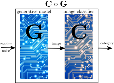Our first definition is of global correctness , it relies on a first key but simple idea, which is to compose a generative model G with an image classifier C : we construct a new neural network C ◦ G by simply rewiring the output of G to the input of C , so C ◦ G represents a distribution over categories. Indeed, it takes as input a random noise and outputs a category. Figure 1: Composition of a generative model with an image classifier <details> <summary>Image 1 Details</summary>  ### Visual Description ## Diagram: Generative Model and Image Classifier Workflow ### Overview The diagram illustrates a two-stage computational pipeline involving a generative model and an image classifier. It depicts the flow of data from random noise through a generative process to produce an image, which is then classified into a category. ### Components/Axes - **Title**: "C ○ G" (centered at the top). - **Left Section**: - Label: "generative model" (above a blue patterned rectangle). - Text: "G" (large black letter centered in the rectangle). - Input: "random noise" (arrow pointing to the left edge of the generative model). - Output: "image" (arrow pointing from the right edge of the generative model to the image classifier). - **Right Section**: - Label: "image classifier" (above a blue patterned rectangle). - Text: "C" (large black letter centered in the rectangle). - Output: "category" (arrow pointing from the right edge of the image classifier). ### Detailed Analysis - **Generative Model**: - Represents a system (denoted by "G") that transforms random noise into structured images. - Visualized with a blue background and white circuit-like patterns, symbolizing neural network architecture. - **Image Classifier**: - Represents a system (denoted by "C") that analyzes images and assigns them to predefined categories. - Shares the same visual style as the generative model, emphasizing parallel computational processes. - **Data Flow**: 1. **Random Noise** → **Generative Model (G)** → **Image** → **Image Classifier (C)** → **Category**. 2. Arrows indicate unidirectional flow, with no feedback loops shown. ### Key Observations - The diagram uses consistent visual motifs (blue background, white circuit patterns) for both components, suggesting they are part of the same system. - The labels "G" and "C" directly correspond to the generative model and classifier, respectively, aligning with common GAN (Generative Adversarial Network) terminology. - No numerical values, scales, or legends are present, indicating this is a conceptual rather than quantitative representation. ### Interpretation This diagram abstractly represents a **Generative Adversarial Network (GAN)** framework: - The **generative model (G)** acts as the "generator," creating synthetic images from random noise. - The **image classifier (C)** acts as the "discriminator," evaluating the authenticity of generated images and assigning categories. - The absence of feedback loops (e.g., adversarial training dynamics) suggests this is a simplified depiction, focusing on the basic workflow rather than iterative optimization processes. - The use of "C ○ G" as the title may symbolize the composition of the two systems in sequence, though the mathematical notation (circle-plus) is unconventional for GANs, which typically emphasize adversarial interaction (G vs. C). No numerical data or trends are present. The diagram serves as a high-level schematic for understanding the roles of generative and classification components in image synthesis pipelines. </details> Definition 1 (Global Correctness) . Given for each c ∈ C a generative model G c for images of category c , we say that the image classifier C is δ -correct with respect to the generative models ( G c ) c ∈ C if for each c ∈ C , $$\mathbb { P } _ { x \sim N ( 0 , 1 ) } ( C \circ G _ { c } ( x ) = c ) \geq 1 - \delta .$$ In words, the probability that for a noise x the image generated (using G c ) is correctly classified (by C ) is at least 1 -δ . ## Assumptions Our definition of global correctness hinges on two properties of generative models: 1. generative models produce a wide variety of images, 2. generative models produce (almost only) realistic images. The first assumption is the reason for the success of generative adversarial networks (GAN) (Goodfellow et al. (2014)). We refer for instance to Karras et al. (2018) and to the attached website thispersondoesnotexist.com for a demo. In our experiments the generative models we used are out of the shelf generative adversarial networks (GAN) (Goodfellow et al. (2014)), with 4 hidden layers of respectively 256, 512 , 1024, and 784 nodes, producing images of single digits. To test the second assumption we performed a first experiment called the manual score experiment . We picked 100 digit images using a generative model and asked 5 individuals to tell for each of them whether they are 'near-perfect', 'perturbed but clearly identifiable', 'hard to identify', or 'rubbish', and which digit they represent. The results are that 96 images were correctly identified; among them 63 images were declared 'near-perfect' by all individuals, with another 26 including 'perturbed but clearly identifiable', and 8 were considered 'hard to identify' by at least one individual yet correctly identified. The remaining 4 were 'rubbish' or incorrectly identified. It follows that against this generative model, we should require an image classifier to be at least . 89-correct, and even . 96-correct to match human perception. ## Algorithm To check whether a classifier is δ -correct, the Monte Carlo integration method is a natural approach: we sample n random noises x 1 , . . . , x n , and count for how many x i 's we have that C ◦ G c ( x ) = c . The central limit theorem states that the ratio of positives over n converges to P x ∼N (0 , 1) ( C ◦ G c ( x ) = c ) as 1 √ n . It follows that n = 10 4 samples gives a 10 -2 precision on this number. In practice, rather than sampling the random noises independently, we form (large) batches and leverage the tensor-based computation, enabling efficient GPU computation. ## 3 Global Robustness We introduce the notion of global robustness, which gives stronger guarantees than global correctness. Indeed, it includes the notion of perturbations for images. The usual notion of robustness, which we call here local robustness , can be defined as follows. Definition 2 (Local Robustness) . We say that the image classifier C is ε -robust around the image y ∈ R d of category c if $$\forall y ^ { \prime } , \, | | y - y ^ { \prime } | | \leq \varepsilon \implies C ( y ^ { \prime } ) = c .$$ In words, all ε -perturbations of y are correctly classified (by C ). One important aspect in this definition is the choice of the norm for the perturbations (here we use the infinity norm). We ignore this as it will not play a role in our definition of robustness. A wealth of techniques have been developed for checking local robustness of neural networks, with state of the art tools being able to handle nets with thousands of neurons. ## Assumptions Our definition of global robustness is supported by the two properties of generative models discussed above in the context of global correctness, plus a third one: 3. generative models produce perturbations of realistic images. To illustrate this we designed a second experiment called the random walk experiment : we perform a random walk on the space of random noises while observing the ensued sequence of images produced by the generative model. More specifically, we pick a random noise x 0 , and define a sequence ( x i ) i ≥ 0 of random noises with x i +1 obtained from x i by adding a small random noise to x i ; this induces the sequence of images ( G ( x i )) i ≥ 0 . The result is best visualised in an animated GIF (see the Github repository), see also the first 16 images in Figure 2. This supports the claim that images produced with similar random noises are (often) close to each other; in other words the generative model is (almost everywhere) continuous. Our definition of global robustness is reminiscent of the provably approximately correct learning framework developed by Valiant (1984). It features two parameters. The first parameter, δ , quantifies the probability that a generative model produces a realistic image. The second parameter, ε , measures the perturbations on the noise, which by the continuity property discussed above transfers to perturbations of the produced images. Definition 3 (Global Robustness) . Given for each c ∈ C a generative model G c for images of category c , we say that the image classifier C is ( ε, δ ) -robust with respect to the generative models ( G c ) c ∈ C if for each c ∈ C , $$e \, l o c a l \quad \mathbb { P } _ { x \sim \mathcal { N } ( 0 , 1 ) } ( \forall x ^ { \prime } , \, | | x - x ^ { \prime } | | \leq \varepsilon \implies C \circ G _ { c } ( x ^ { \prime } ) = c ) \geq 1 - \delta .$$ In words, the probability that for a noise x , all ε -perturbations of x generate (using G ) images correctly classified (by C ) is at least 1 -δ . ## Algorithm To check whether a classifier is ( ε, δ )-robust, we extend the previous ideas using the Monte Carlo integration: we sample n random noises x 1 , . . . , x n , and count for how many x i 's the following property holds: $$\forall x , \, | | x _ { i } - x | | \leq \varepsilon \implies C \circ G _ { c } ( x ) = c .$$ The central limit theorem states that the ratio of positives over n converges to $$\mathbb { P } _ { x \sim \mathcal { N } ( 0 , 1 ) } ( \forall x ^ { \prime } , | | x - x ^ { \prime } | | \leq \varepsilon \implies C \circ G _ { c } ( x ^ { \prime } ) = c )$$ as 1 √ n . As before, it follows that n = 10 4 samples gives a 10 -2 precision on this number. In other words, checking global robustness reduces to combining Monte Carlo integration with checking local robustness. ## 4 Experiments The code for all experiments can be found on the Github repository https://github.com/mohitiitb/ NeuralNetworkVerification\_GlobalRobustness . All experiments are presented in Jupyter notebook format with pre-trained models to be easily reproduced. Our experiments are all reproduced on the drop-in Fashion-MNIST dataset (Xiao et al. (2017)), obtaining similar results. We report on experiments designed to assess the benefit of these two notions, whose common denominator is to go from a local property to a global one by composing with a generative model. We first evaluate the global correctness of several image classifiers, showing that it provides a finer way of evaluating them than the usual test set. We then turn to global robustness and show how the negation of robustness can be witnessed by realistic adversarial examples. The second set of experiments addresses the fact that both global correctness and robustness notions depend on the choice of a generative model. We show that this dependence can be made small, but that it can also be used for refining the correctness and robustness notions. ## 8 8 8 8 8 8 8 8 8 8 8 8 8 Figure 2: The random walk experiment ## Choice of networks In all the experiments, our base case for image classifiers have 3 hidden layers of increasing capacities: the first one, referred to as 'small', has layers with (32 , 64 , 200) (number of nodes), 'medium' corresponds to (64 , 128 , 256), and 'large' to (64 , 128 , 512). The generative model are as described above, with 4 hidden layers of respectively 256, 512 , 1024, and 784 nodes. For each of these three architectures we either use the standard MNIST training set (6,000 images of each digit), or an augmented training set (24,000 images), obtained by rotations, shear, and shifts. The same distinction applies to GANs: the 'simple GAN' uses the standard training set, and the 'augmented GAN' the augmented training set. Finally, we work with two networks obtained through robust training procedures. The first one was proposed by M¸ adry et al. (2018) for the MNIST Adversarial Example Challenge (the goal of the challenge was to find adversarial examples, see below), and the second one was defined by Papernot et al. (2016) through the process of defense distillation. ## Evaluating Global Correctness We evaluated the global correctness of all the image classifiers mentioned above against simple and augmented GANs, and reported the results in the table below. The last column is the usual validation procedure, meaning the number of correct classification on the MNIST test set of 10,000 images. They all perform very well, and close to perfectly (above 99%), against this metric, hence cannot be distinguished. Yet the composition with a generative model reveals that their performance outside of the test set are actually different. It is instructive to study the outliers for each image classifier, i.e. the generated images which are incorrectly classified. We refer to the Github repository for more experimental results along these lines. ## Finding Realistic Adversarial Examples Checking the global robustness of an image classifier is out of reach for state of the art verification tools. Indeed, a single robustness check on a medium size net takes somewhere between dozens of seconds to a | Classifier | simple GAN | augmented GAN | test set | |----------------------------|----------------------------|----------------------------|----------------------------| | Standard training set | Standard training set | Standard training set | Standard training set | | small | 98.89 | 92.82 | 99.79 | | medium | 99.15 | 93.16 | 99.76 | | large | 99.38 | 93.80 | 99.80 | | Augmented training set | Augmented training set | Augmented training set | Augmented training set | | small | 97.84 | 95.2 | 99.90 | | medium | 99.11 | 96.53 | 99.86 | | large | 99.25 | 97.66 | 99.84 | | Robust training procedures | Robust training procedures | Robust training procedures | Robust training procedures | | M¸ adry et al. (2018) | 98.87 | 93.17 | 99.6 | | Papernot et al. (2016) | 99.64 | 94.78 | 99.17 | few minutes, and to get a decent approximation we need to perform tens of thousands local robustness checks. Hence with considerable computational efforts we could analyse one image classifier, but could not perform a wider comparison of different training procedures and influence on different aspects. Thus our experiments focus on the negation of robustness, which is finding realistic adversarial examples, that we define now. Definition 4 (Realistic Adversarial Example) . An ε -realistic adversarial example for an image classifier C with respect to a generative model G is an image G ( x ) such that there exists another image G ( x ′ ) with $$| | x - x ^ { \prime } | | \leq \varepsilon a n d \, C \circ G ( x ) \neq C \circ G ( x ^ { \prime } )$$ In words, x and x ′ are two ε -close random noises which generate images G ( x ) and G ( x ′ ) that are classified differently by C . Note that a realistic adversarial example is not necessarily an adversarial example: the images G ( x ) and G ( x ′ ) may differ by more than ε . However, this is the assumption 3. discussed when defining global robustness, if x and x ′ are close, then typically G ( x ) and G ( x ′ ) are two very resemblant images, so the two notions are indeed close. We introduce two algorithms for finding realistic adversarial examples, which are directly inspired by algorithms developed for finding adversarial examples. The key difference is that realistic adversarial examples are searched by analysing the composed network C ◦ G . Let us consider two digits, for the sake of explanation, 3 and 8. We have a generative model G 8 generating images of 8 and an image classifier C . The first algorithm is a black-box attack , meaning that it does not have access to the inner structure of the networks and it can only simulate them. It consists in sampling random noises, and performing a local search for a few steps. From a random noise x , we inspect the random noise x + δ for a few small random noises δ , and choose the random noise x ′ maximising the score of 3 by the net C ◦ G 8 , written C ◦ G 8 ( x i )[3] in the pseudocode given in Algorithm 1. The algorithm is repeatedly run until a realistic adversarial example is found. Algorithm 1: The black-box attack for the digits 3 and 8. ``` ``` The second algorithm is a white-box attack , meaning that it uses the inner structure of the networks. It is similar to the previous one, except that the local search is replaced by a gradient ascent to maximise the score of 3 by the net C ◦ G 8 . In other words, instead of choosing a direction at random, it follows the gradient to maximise the score. It is reminiscent of the projected gradient descent (PGD) attack, but performed on the composed network. The pseudocode is given in Algorithm 2. Both attacks successfully find realistic adversarial examples within less than a minute. The adjective 'realistic', which is subjective, is justified as follows: most attacks constructing adversarial examples create un- Algorithm 2: The white-box attack for the digits 3 ``` and 8. ``` ``` Data: A generative model G$_{8}$ and an image classifier C. A parameter $\varepsilon > 0$. 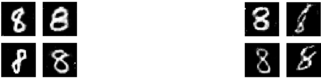N$_step$ <- 16 (number of steps) \alpha <- \frac{\varepsilon N_{step} } { (step)} x$_0 ~ $N_{0,1} ) for i = 0 to N$_step - 1 do \ifcase C \circ G$_8(x_i)[3] then return x_0 ( $\varepsilon -realistic adversarial example) ``` realistic images by adding noise or modifying pixels, while with our definition the realistic adversarial examples are images produced by the generative model, hence potentially more realistic. See Figure 3 for some examples. ## On the Dependence on the Generative Model Both global correctness and robustness notions are defined with respect to a generative model. This raises a question: how much does it depend on the choice of the generative model? To answer this question we trained two GANs using the exact same training procedure but with two disjoint training sets, and used the two GANs to evaluate several image classifiers. The outcome is that the two GANs yield sensibly the same results against all image classifiers. This suggests that the global correctness indeed does not depend dramatically on the choice of the generative model, provided that it is reasonably good and well-trained. We refer to the Github repository for a complete exposition of the results. Since the training set of the MNIST dataset contains 6,000 images of each digit, splitting it in two would not yield two large enough training sets. Hence we used the extended MNIST (EMNIST) dataset Cohen et al. (2017), which provided us with (roughly) 34,000 images of each digit, hence two disjoint datasets of about 17,000 images. ## On the Influence of Data Augmentation Data augmentation is a classical technique for increasing the size of a training set, it consists in creating new training data by applying a set of mild transformations to the existing training set. In the case of digit images, common transformations include rotations, shear, and shifts. Unsurprisingly, crossing the two training sets, e.g. using the standard training set for the image classifier and an augmented one for the generative model yields worse results than when using the same training set. More interestingly, the robust networks M¸ adry et al. (2018); Papernot et al. (2016), which are trained using an improved procedure but based on the standard training set, perform well against generative models trained on the augmented training set. In other words, one outcome of the improved training procedure is to better capture the natural image transformations, even if they were never used in training. ## 5 Conclusions We defined two notions: global correctness and global robustness, based on generative models, aiming at quantifying the usability of an image classifier. We performed some experiments on the MNIST dataset to understand the merits and limits of our definitions. An important challenge lies ahead: to make the verification of global robustness doable in a reasonable amount of time and computational effort. ## Bibliography Dan Ciregan, Ueli Meier, and Juergen Schmidhuber. Multi-column deep neural networks for image classification. In IEEE Conference on Computer Vision and Pattern Recognition (CCVPR) , pages 3642-3649, June 2012. doi: 10.1109/CVPR. 2012.6248110. URL https://ieeexplore.ieee. org/document/6248110 . Gregory Cohen, Saeed Afshar, Jonathan Tapson, and Andr´ e van Schaik. EMNIST: an extension of MNIST to handwritten letters. CoRR , abs/1702.05373, 2017. URL http://arxiv.org/abs/1702.05373 . Timon Gehr, Matthew Mirman, Dana DrachslerCohen, Petar Tsankov, Swarat Chaudhuri, and Martin T. Vechev. AI2: safety and robustness certification of neural networks with abstract interpretation. In IEEE Symposium on Security and Privacy (SP) , pages 3-18, 2018. doi: 10.1109/SP.2018.00058. URL https://doi.org/10.1109/SP.2018.00058 . Ian J. Goodfellow, Jean Pouget-Abadie, Mehdi Mirza, Bing Xu, David Warde-Farley, Sherjil Ozair, Aaron C. Courville, and Yoshua Bengio. Generative adversarial nets. In Conference on Neural Information Processing Systems (NIPS) , pages 26722680, 2014. URL http://papers.nips.cc/paper/ 5423-generative-adversarial-nets . Divya Gopinath, Guy Katz, Corina S. Pasareanu, and Clark Barrett. Deepsafe: A data-driven approach for assessing robustness of neural networks. In Symposium on Automated Technology for Verification and Analysis (ATVA) , pages 3-19, 2018. Figure 3: Examples of realistic adversarial examples. On the left hand side, against the smallest net, and on the right hand side, against M¸ adry et al. (2018) <details> <summary>Image 2 Details</summary>  ### Visual Description ## Handwritten Digit Classification Examples ### Overview The image displays a 2x4 grid of eight handwritten digit samples on a black background. The digits are rendered in white, with variations in stroke thickness and curvature. No additional labels, axes, or legends are present. ### Components/Axes - **Grid Structure**: - 2 rows (top and bottom) - 4 columns (left to right) - **Digit Representation**: - All digits are handwritten, with no standardized font or style. - Background: Solid black (no grid lines or separators). - **Color Scheme**: - Digits: White (high contrast against black background). - No other colors or annotations. ### Detailed Analysis 1. **Top Row (Left to Right)**: - **Position 1 (Top-Left)**: Digit "8" with a closed loop and two horizontal strokes. - **Position 2 (Top-Middle-Left)**: Digit "8" with a slightly open lower loop. - **Position 3 (Top-Middle-Right)**: Digit "8" with a thicker upper stroke. - **Position 4 (Top-Right)**: Digit "8" with a more angular, less curved form. 2. **Bottom Row (Left to Right)**: - **Position 5 (Bottom-Left)**: Digit "8" with a minimalist, almost circular shape. - **Position 6 (Bottom-Middle-Left)**: Digit "8" with a pronounced diagonal stroke. - **Position 7 (Bottom-Middle-Right)**: Digit "8" with a wavy, irregular lower loop. - **Position 8 (Bottom-Right)**: Digit "6" with a single loop and a short tail. ### Key Observations - **Dominance of "8"**: Seven out of eight digits are "8", emphasizing its prevalence in the dataset. - **Single "6" Anomaly**: The bottom-right digit ("6") is the only non-"8", suggesting a focus on distinguishing similar shapes. - **Handwriting Variability**: Significant differences in stroke thickness, curvature, and closure (e.g., open vs. closed loops in "8"). ### Interpretation This image likely serves as a test case for handwritten digit recognition systems. The variations in "8" demonstrate challenges in normalizing handwriting styles, while the inclusion of a "6" highlights the importance of distinguishing visually similar digits. The lack of standardization in stroke patterns suggests real-world data complexity, where models must account for human variability rather than rigid templates. The single "6" may act as a stress test for algorithms trained primarily on "8"-dominated datasets. </details> doi: 10.1007/978-3-030-01090-4 \ 1. URL https: //doi.org/10.1007/978-3-030-01090-4\_1 . Xiaowei Huang, Marta Kwiatkowska, Sen Wang, and Min Wu. Safety verification of deep neural networks. In Computer-Aided Verification (CAV) , pages 3-29, 2017. doi: 10.1007/ 978-3-319-63387-9 \ 1. URL https://doi.org/10. 1007/978-3-319-63387-9\_1 . Tero Karras, Samuli Laine, and Timo Aila. A stylebased generator architecture for generative adversarial networks. CoRR , abs/1812.04948, 2018. URL http://arxiv.org/abs/1812.04948 . Guy Katz, Clark W. Barrett, David L. Dill, Kyle Julian, and Mykel J. Kochenderfer. Reluplex: An efficient SMT solver for verifying deep neural networks. In Computer-Aided Verification (CAV) , pages 97-117, 2017. doi: 10.1007/ 978-3-319-63387-9 \ 5. URL https://doi.org/10. 1007/978-3-319-63387-9\_5 . Guy Katz, Derek A. Huang, Duligur Ibeling, Kyle Julian, Christopher Lazarus, Rachel Lim, Parth Shah, Shantanu Thakoor, Haoze Wu, Aleksandar Zeljic, David L. Dill, Mykel J. Kochenderfer, and Clark W. Barrett. The marabou framework for verification and analysis of deep neural networks. In ComputerAided Verification (CAV) , pages 443-452, 2019. doi: 10.1007/978-3-030-25540-4 \ 26. URL https: //doi.org/10.1007/978-3-030-25540-4\_26 . Aleksander M¸ adry, Aleksandar Makelov, Ludwig Schmidt, Dimitris Tsipras, and Adrian Vladu. Towards deep learning models resistant to adversarial attacks. In International Conference on Learning Representations (ICLR) , 2018. URL https: //openreview.net/forum?id=rJzIBfZAb . Matthew Mirman, Timon Gehr, and Martin T. Vechev. Differentiable abstract interpretation for provably robust neural networks. In International Conference on Machine Learning (ICML) , pages 3575-3583, 2018. URL http://proceedings.mlr. press/v80/mirman18b.html . Nicolas Papernot, Patrick D. McDaniel, Xi Wu, Somesh Jha, and Ananthram Swami. Distillation as a defense to adversarial perturbations against deep neural networks. In IEEE Symposium on Security and Privacy (SP) , pages 582-597, 2016. doi: 10.1109/SP.2016.41. URL https://doi.org/10. 1109/SP.2016.41 . Christian Szegedy, Wojciech Zaremba, Ilya Sutskever, Joan Bruna, Dumitru Erhan, Ian J. Goodfellow, and Rob Fergus. Intriguing properties of neural networks. In International Conference on Learning Representations (ICLR) , 2014. URL http: //arxiv.org/abs/1312.6199 . Leslie G. Valiant. A theory of the learnable. Communications of the ACM , 27(11):1134-1142, 1984. doi: 10.1145/1968.1972. URL https://doi.org/ 10.1145/1968.1972 . Li Wan, Matthew Zeiler, Sixin Zhang, Yann Le Cun, and Rob Fergus. Regularization of neural networks using dropconnect. In International Conference on Machine Learning (ICML) , volume 28, pages 1058-1066, 2013. URL http://proceedings.mlr. press/v28/wan13.html . Tsui-Wei Weng, Huan Zhang, Hongge Chen, Zhao Song, Cho-Jui Hsieh, Luca Daniel, Duane S. Boning, and Inderjit S. Dhillon. Towards fast computation of certified robustness for relu networks. In International Conference on Machine Learning (ICML) , pages 5273-5282, 2018. URL http://proceedings. mlr.press/v80/weng18a.html . Chaowei Xiao, Bo Li, Jun-Yan Zhu, Warren He, Mingyan Liu, and Dawn Song. Generating adversarial examples with adversarial networks. In Proceedings of the Twenty-Seventh International Joint Conference on Artificial Intelligence (IJCAI) , pages 3905-3911, 2018. doi: 10.24963/ijcai.2018/ 543. URL https://doi.org/10.24963/ijcai. 2018/543 . Han Xiao, Kashif Rasul, and Roland Vollgraf. Fashion-MNIST: a novel image dataset for benchmarking machine learning algorithms. CoRR , abs/1708.07747, 2017. URL http://arxiv.org/ abs/1708.07747 .