1912.06101v1

## The PlayStation Reinforcement Learning Environment (PSXLE) ## Carlos Purves, C˘ at˘ alina Cangea, Petar Veliˇ ckovi´ c Department of Computer Science and Technology University of Cambridge {cp614, catalina.cangea, petar.velickovic}@cst.cam.ac.uk ## Abstract We propose a new benchmark environment for evaluating Reinforcement Learning (RL) algorithms: the PlayStation Learning Environment (PSXLE), a PlayStation emulator modified to expose a simple control API that enables rich game-state representations. We argue that the PlayStation serves as a suitable progression for agent evaluation and propose a framework for such an evaluation. We build an action-driven abstraction for a PlayStation game with support for the OpenAI Gym interface and demonstrate its use by running OpenAI Baselines . ## 1 Introduction Reinforcement Learning (RL) describes a form of machine learning in which an agent learns how to interact with an environment through the acquisition of rewards that are chosen to encourage good behaviours and penalise harmful ones. The environment is described to the agent at each point in time by a state encoding . A well-trained agent should use this encoding to select its next action as one that maximises its long-term cumulative reward. This model of learning has proved effective in many real-world environments, including in self-driving cars [1], traffic control [2], advertising [3] and robotics [4]. An important advance in RL research came with the development of Deep Q-Networks (DQN), in which agents utilise deep neural networks to interpret complex state spaces. Increased attention towards RL in recent years has led to further advances such as Double DQN [5], Prioritised Experience Replay [6] and Duelling Architectures [7] bringing improvements over DQN. Policy-based methods such as A3C have brought further improvements [8] and asynchronous methods to RL. In order to quantify the success of these learning algorithms and to demonstrate improvements in new approaches, a common evaluation methodology is needed. Computer games are typically used to fulfil this role, providing practical advantages over other types of environments: episodes are reproducible , due to the lack of uncontrollable stochasticity; they offer comparatively low-dimensional state encodings; and the notion of a 'score' translates naturally into one of a 'reward'. The use of computer games also serves a more abstract purpose: to court public interest in RL research. Describing the conclusions of research in terms of a player's achievement in a computer game makes the work more approachable and improves its comprehensibility, as people can utilise their own experience of playing games as a baseline for comparison. In 2015, Mnih et al. [9] used the Atari-2600 console as an environment in which to evaluate DQN. Their agent outperformed human expert players in 22 out of the 49 games that were used in training. In 2016, OpenAI announced OpenAI Gym [10], which allows researchers and developers to interface with games and physical simulations in a standardised way through a Python library. Gym now represents the de-facto standard evaluation method for RL algorithms [11]. It includes, amongst others [12], several Atari-2600 games which utilise Arcade Learning Environment (ALE) [13] to interface with a console emulation. One of the most important considerations in developing successful RL methods in complex environments is the choice of state encoding . This describes the relationship between the state of an environment and the format of the data available to the agent. For a human playing a game, 'state' can mean many things, including: the position of a character in a world, how close enemies are, the remaining time on a clock or the set of previous actions. While these properties are easy for humans to quantify, RL environments usually do not encode them explicitly for two reasons. Firstly, doing so would simplify the problem too much, permitting reliance on a human understanding of the environment-something which should ideally be approximated through learning. Secondly, it does not allow agents to generalise, since each game's state will be described by different properties. Rather, game-based RL environments typically consider the 'state' to be an element of some common state space . Common examples of such spaces are the set of a console's possible display outputs or its RAM contents. Until now, RL research has seen little exploration of the use of sound effects in state encodings. This is clearly not due to a lack of methods for processing audio data; there is substantial research precedent in the areas of speech recognition [14], audio in affective computing [15] and unsupervised approaches to music genre detection [16]. A discussion about richer state encodings is particularly pertinent given the success of existing RL approaches within conventional environments. A significant gap exists between the richness and complexity of such environments and those representing the eventual goal of RL: real-world situations with naturally many-dimensional state spaces. To help narrow this gap, this paper introduces the PlayStation Reinforcement Learning Environment (PSXLE): a toolkit for training agents to play Sony PlayStation 1 games. PSXLE is designed to follow from the standard set by ALE and enable RL research using more complex environments and state encodings. It increases the complexity of the games that can be used within a framework such as OpenAI Gym, due to the significant hardware differences between the consoles. PSXLE utilises this additional complexity by exposing raw audio output from the console alongside RAM and display contents. We implement an OpenAI Gym interface for the PlayStation game Kula World and use OpenAI Baselines to evaluate the performance of two popular RL algorithms with it. 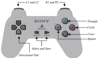## 2 PlayStation Figure 1: The PlayStation controller, highlighting its 14 buttons. <details> <summary>Image 1 Details</summary>  ### Visual Description \n ## Diagram: PlayStation Controller Layout ### Overview The image is a diagram illustrating the layout of a PlayStation controller. It depicts a top-down view of the controller, with labels pointing to various buttons and components. The diagram is primarily for identifying the location and names of the controller's features. ### Components/Axes The diagram labels the following components: * **L1 and L2**: Located on the left shoulder of the controller. * **R1 and R2**: Located on the right shoulder of the controller. * **Triangle**: A blue triangle-shaped button. * **Circle**: A red circle-shaped button. * **Cross**: A blue cross-shaped button. * **Square**: A pink square-shaped button. * **Directional Pad**: Located on the left side of the controller. * **Select and Start**: Two buttons located centrally, below the PlayStation logo. * **PlayStation Logo**: Centrally located on the controller face. * **SONY**: Brand name located above the PlayStation logo. ### Detailed Analysis or Content Details The diagram provides a static representation of the controller's layout. There are no numerical values or trends to analyze. The labels are directly associated with the corresponding buttons/components on the controller image. * **Shoulder Buttons:** L1 and L2 are positioned on the upper-left, while R1 and R2 are on the upper-right. * **Face Buttons:** The Triangle, Circle, Cross, and Square buttons are arranged in a diamond pattern on the right side of the controller. * **Central Buttons:** The Select and Start buttons are positioned below the PlayStation logo. * **Directional Pad:** The directional pad is located on the left side of the controller. ### Key Observations The diagram clearly identifies all the major buttons and components of a standard PlayStation controller. The layout is symmetrical, with the shoulder buttons and face buttons mirroring each other. The PlayStation logo and brand name are prominently displayed. ### Interpretation The diagram serves as a visual guide for understanding the physical layout of a PlayStation controller. It is useful for new users learning the controller's functions or for reference when discussing controller configurations. The diagram does not provide any information about the controller's functionality or technical specifications, only its physical arrangement. The diagram is a simple, direct representation of the controller's design, intended for easy identification of its components. </details> The Sony PlayStation 1 (sometimes PSX or PlayStation ) is a console first released by Sony Computer Entertainment in 1994. It has 2 megabytes of RAM, 16.7 million displayable colours and a 33.9 MHz CPU, which contrasts with the Atari-2600's 128 bytes of RAM, 128 displayable colours and a 1.19MHz CPU. Since its launch, the number of titles available for the PlayStation has grown to almost 8000 worldwide, more than the 500 that are available for the Atari-2600 console. PlayStation games are controlled using a handheld controller, shown in Figure 1. The controller has 14 buttons, with Start typically used to pause a game. 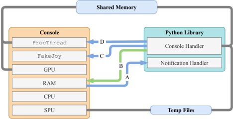Figure 2: A visualisation of the Inter-Process Communication used in PSXLE. Pipes are coloured green, FIFO queues are coloured blue and Unix fopen calls are coloured grey. A is used to notify the PSXLE Python library that parts of memory have changed and that events like load\_state and save\_state have completed. B , representing standard input stdin , is used to communicate which regions of memory the console should watch. C is used to send simulated button presses to the console. D sends instructions to the console, such as loading and saving state or loading an ISO. <details> <summary>Image 2 Details</summary>  ### Visual Description \n ## Diagram: System Architecture - Console and Python Library Interaction ### Overview The image depicts a system architecture diagram illustrating the interaction between a "Console" component and a "Python Library" component. Data flow is represented by colored arrows, and the diagram also shows connections to "Shared Memory" and "Temp Files". The diagram appears to be a high-level overview of how the console interacts with a Python library for handling console operations and notifications. ### Components/Axes The diagram consists of the following components: * **Console (Peach-colored rectangle):** Contains the following sub-components: * ProcThread * FakeJoy * GPU * RAM * CPU * SPU * **Python Library (Light Blue rectangle):** Contains the following sub-components: * Console Handler * Notification Handler * **Shared Memory (Light Blue rounded rectangle):** Located at the top of the diagram. * **Temp Files (Light Blue rounded rectangle):** Located at the bottom of the diagram. * **Arrows:** Represent data flow, labeled A, B, C, and D. The arrows are colored: Green, Blue, and a combination of Green and Blue. ### Detailed Analysis or Content Details The diagram shows the following data flow: * **Arrow A (Green):** Originates from the RAM component within the Console and connects to the Console Handler within the Python Library. * **Arrow B (Blue):** Originates from the CPU component within the Console and connects to the Notification Handler within the Python Library. * **Arrow C (Green):** Originates from the FakeJoy component within the Console and connects to the Console Handler within the Python Library. * **Arrow D (Blue):** Originates from the ProcThread component within the Console and connects to the Console Handler within the Python Library. Both the Console and the Python Library are connected to "Shared Memory" and "Temp Files" via gray lines, indicating a broader system-level interaction. The connections to Shared Memory and Temp Files are not labeled with specific data flow indicators. ### Key Observations The diagram highlights a clear separation of concerns between the Console and the Python Library. The Console appears to handle low-level hardware interactions (GPU, RAM, CPU, SPU), while the Python Library provides higher-level handling of console operations and notifications. The use of different colored arrows suggests different types of data or operations being handled by each connection. The Console's components are listed vertically, while the Python Library's components are listed horizontally. ### Interpretation This diagram likely represents a system where a console application interacts with a Python-based backend for handling console-related tasks. The Console provides the raw input and hardware access, while the Python Library processes this input and manages notifications. The use of Shared Memory and Temp Files suggests that data is being exchanged between the Console and the Python Library outside of the direct connections shown by the colored arrows. The diagram suggests a modular architecture, where the Console and Python Library can be developed and maintained independently. The specific data flow indicated by the arrows (A, B, C, D) likely represents different types of console events or commands being processed by the Python Library. For example, RAM data might be sent to the Console Handler for rendering, while CPU events might trigger notifications. The "FakeJoy" component suggests the system may be simulating joystick input, sending this data to the Console Handler. The "ProcThread" component likely handles process-related tasks, sending information to the Console Handler. The diagram does not provide quantitative data or specific details about the data being exchanged, but it offers a valuable overview of the system's architecture and the relationships between its key components. 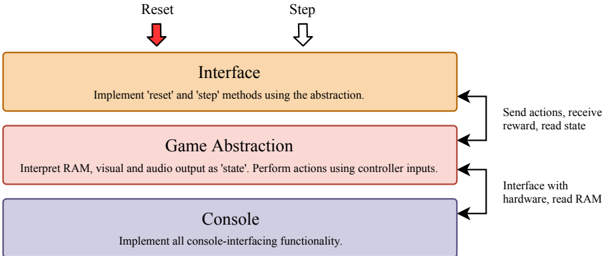</details> ## 3 Implementation PSXLE is built using a fork of PCSX-R 1 , an open-source emulator created in 2009. We made modifications to the source of PCSX-R by adding simple Inter-Process Communication (IPC) toolsthe structure of which is shown in Figure 2-to simulate controller inputs and read console output through an external interface. The PSXLE Python library uses these tools to provide a simple, game-agnostic PlayStation console interface. To specialise the environment to a certain game and implement an interface such as OpenAI Gym, a customised environment stack can be created that abstracts console-level functions across two layers. Figure 3 visualises the structure of such a stack. Specialisation to individual games occurs within the 'game abstraction' component, which uses the Console API to translate game actions (such as 'move forwards') into console functions (such as 'press up'). The Console API supports four primary forms of interaction: ## · General: - -run and kill control the executing process of the emulator; - -freeze and unfreeze will freeze and unfreeze the emulator's execution, respectively; - -speed is a property of Console which, when set, will synchronously set the speed of execution of the console, expressed as a percentage relative to default speed. ## · Controller: - -hold\_button and release\_button simulate a press down and release of a given controller button-referred to here as control events ; - -touch\_button holds, pauses for a specified amount of time and then releases a button; - -delay\_button adds a (millisecond-order) delay between successive control events ## · RAM: - -read\_bytes and write\_byte directly read from and write to console memory; - -add\_memory\_listener and clear\_memory\_listeners control which parts of the console's memory should have asynchronous listeners attached when the console runs; - -sleep\_memory\_listener and wake\_memory\_listener tell the console which listeners are active. - Audio/Visual: 1 Available at https://github.com/pcsxr/PCSX-Reloaded/ - -start\_recording\_audio and stop\_recording\_audio control when the console should record audio and when it should stop; - -get\_screen synchronously returns an np.array of the console's instantaneous visual output. Example usage of the PSXLE interface can be found in Appendix A. Figure 3: The proposed architecture for PlayStation RL environments includes three components: the interface , which allows agents to perform actions and receive feedback; the game abstraction , which translates game actions into controller inputs and console state (visual, audio and RAM) into state representations; and the console , which handles communication with the emulator. <details> <summary>Image 3 Details</summary>  ### Visual Description \n ## Diagram: System Architecture - Interface, Game Abstraction, and Console ### Overview The image depicts a layered system architecture diagram illustrating the interaction between an Interface, a Game Abstraction layer, and a Console layer. Arrows indicate the flow of control and data between these layers. The diagram appears to represent a software or system design, likely related to game development or simulation. ### Components/Axes The diagram consists of three rectangular blocks stacked vertically, representing the three layers: * **Interface:** (Top layer, light orange color) * **Game Abstraction:** (Middle layer, light red color) * **Console:** (Bottom layer, light blue color) Two arrows are positioned above the Interface layer: * **Reset:** (Red arrow pointing downwards) * **Step:** (Grey arrow pointing downwards) Text labels are associated with each layer, describing their function. Arrows connecting the layers indicate data flow and are labeled with descriptions of the interaction. ### Detailed Analysis or Content Details The diagram shows a hierarchical structure with information flowing downwards and upwards. * **Interface Layer:** * Text: "Implement 'reset' and 'step' methods using the abstraction." * Receives input from "Reset" and "Step" actions. * Sends actions, receives reward, and reads state to the "Game Abstraction" layer. * **Game Abstraction Layer:** * Text: "Interpret RAM, visual and audio output as 'state'. Perform actions using controller inputs." * Receives actions, reward, and state from the "Interface" layer. * Interfaces with hardware and reads RAM to the "Console" layer. * **Console Layer:** * Text: "Implement all console-interfacing functionality." * Receives hardware interface and RAM read requests from the "Game Abstraction" layer. The arrows connecting the layers are labeled as follows: * Interface to Game Abstraction: "Send actions, receive reward, read state" * Game Abstraction to Console: "Interface with hardware, read RAM" ### Key Observations The diagram emphasizes a clear separation of concerns between the layers. The "Interface" layer provides the high-level control (reset and step), the "Game Abstraction" layer handles the game logic and state, and the "Console" layer manages the low-level hardware interaction. The flow of control is primarily top-down, with the Interface initiating actions and the Console providing the underlying functionality. ### Interpretation This diagram illustrates a common architectural pattern used in game development and simulation environments. The separation into these layers allows for modularity, reusability, and easier testing. The "Interface" layer acts as an abstraction, allowing different interfaces (e.g., a human player, an AI agent) to interact with the game without needing to know the details of the underlying implementation. The "Game Abstraction" layer encapsulates the game logic and state, while the "Console" layer handles the platform-specific details. The "Reset" and "Step" actions suggest a discrete-time simulation or game loop. "Reset" likely initializes the game to a starting state, while "Step" advances the simulation by one time step. The flow of data (actions, rewards, state) between the layers is crucial for the game to function correctly. The diagram suggests a system where the Interface provides commands, the Game Abstraction processes them and updates the state, and the Console provides the necessary hardware support. </details> ## 4 Game abstraction OpenAI Gym environments expose three methods: reset , which restarts an episode and returns the initial state; step , which takes an action as an argument and performs it within the environment; and render , which renders the current state to a window, or as text. The step function takes an integer representing an action and returns a tuple containing: state , which is the value of the state of the system after an action has taken place; reward , which gives the reward gained by performing a certain action; done , which is a Boolean value indicating whether the episode has finished; and info , which gives extra information about the environment. Gym requires that these methods return synchronously. There are two possible approaches to deriving this synchrony with PlayStation games. Firstly, the environment could exercise granular control over the execution of the console, choosing how many frames to skip for each move. This approach is common and is used to implement the <details> <summary>Image 4 Details</summary>  ### Visual Description \n ## Diagram: State Transitions with Value Changes ### Overview The image depicts a linear sequence of states, each represented by a rectangular block. Arrows indicate transitions between these states, accompanied by a numerical value "+4" or "-4". The diagram illustrates a system undergoing changes in state, with each transition involving a modification of a value. ### Components/Axes The diagram consists of the following components: * **States:** Represented by rectangular blocks. Three states are explicitly labeled. * **Transitions:** Represented by curved arrows connecting the states. * **Value Change:** Each transition arrow is labeled with either "+4" or "-4", indicating the change in value during the transition. * **Labels:** The word "State" appears three times, labeling sections of the diagram. ### Detailed Analysis or Content Details The diagram shows a series of states connected by transitions. The transitions alternate between adding 4 and subtracting 4. * The first state consists of 5 blocks. The transition from the first block to the second is labeled "+4". * The second state consists of 5 blocks. The transition from the second block to the third is labeled "-4". * The third state consists of 5 blocks. The transition from the third block to the fourth is labeled "+4". * This pattern of "+4" and "-4" transitions continues across the entire diagram. * The diagram shows a total of 15 blocks representing states. ### Key Observations The diagram demonstrates a cyclical pattern of value changes. The transitions alternate between adding and subtracting a constant value (4). The diagram does not provide any initial or final state values, only the changes between states. ### Interpretation The diagram likely represents a simplified model of a system where a value is repeatedly incremented and decremented. This could represent a counter, a signal strength, or any other measurable quantity. The "states" could represent discrete time steps or distinct configurations of the system. The consistent "+4" and "-4" transitions suggest a predictable and controlled process. The diagram does not provide information about the underlying mechanism driving these changes, or the purpose of the state transitions. It is a purely visual representation of a value fluctuating between states. 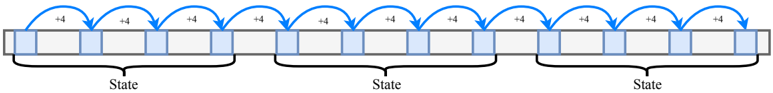</details> (a) A visualisation of frame skip and frame stacking. In [9], only every fourth frame is considered and of those, every four frames are combined (stacked) into a single state representation. New frames are requested by the Python library upon each action, making this approach synchronous. <details> <summary>Image 5 Details</summary>  ### Visual Description Icon/Small Image (771x51) </details> (b) An asynchronous approach to frame skipping. In environments where actions are long or have variable length, the state transition occurs asynchronously. The transition ends once the immediate effects of the associated action have ceased. Figure 4: A comparison of the state-delimiting techniques used in [9] and those used in this paper. Atari-2600 environments in Gym. In cases where a simple snapshot of the environment would leave ambiguity (such as when the motion of an object could be in several directions), consecutive frames may be stacked to produce a corresponding state encoding. Frame skipping works well for simple games, but is not always suitable if moves can take a variable amount of time to finish. If the skip is less than the number of frames a move takes to finish, the agent may choose its next action before a previous move has finished. In many games, this would lead to the chosen action not being completed properly. If the environment was to skip significantly more frames than required, the agent would unnecessarily incur a delay in making moves. A second approach would be to allow the console to run asynchronously for the duration of each move, with an associated condition that signifies the move being over. For example, a move that involves collecting a valuable item might be 'finished' once a player's score has changed. To the agent, the move would begin when step was called and end as soon as the score had increased. This approach is easy to implement with PSXLE, using memory listeners that respond to changes in RAM. These approaches are contrasted in Figure 4. ## 5 Kula World Kula World is a game developed by Game Design Sweden A.B. and released in 1998. It involves controlling a ball within a world that contains a series of objects. The world consists of a platform on which the ball can move. An object can be a coin, a piece of fruit or a key, each of which are collected when a player moves into them. The ball is controlled through the use of the directional pad and the cross button shown in Figure 1. Pressing the right or left directional button rotates the direction of view 90 degrees clockwise or anti-clockwise about the line perpendicular to the platform. Pressing the up directional button moves the player forwards on the platform, in the direction that the camera is facing. Pressing the cross button makes the ball jump, this can be pressed simultaneously with the forward directional button to make the ball jump forwards . Jumping forwards moves the player two squares forwards, over the square in front of it. If the player jumps onto a square that doesn't exist, the game will end. ## 5.1 Actions The definition of the action space for Kula World is relatively simple. We omitted the jump action since this served no purpose within the levels that were tested. In total, the action space is given by: <!-- formula-not-decoded --> There is a clock on each level, which counts down in seconds from a level-specific start value. To complete a level, the player must pick up all of the keys and move to a goal square before the clock reaches zero. Collecting objects gains points, which are added to the player's score for the level. It is not suitable to employ frame skipping in Kula World, since moves can vary in length. A jump, for example, takes roughly a second longer than a camera rotation. The duration of moves can also depend on the specific state of a level; for example, moving forwards to collect a coin takes longer than moving forwards without collecting a coin. This is a problem since a move cannot be carried out while another is taking place. Further, since the logic for the game takes place within the CPU of the console, it is not possible in general to predict the duration of a move prior to it finishing. Instead, the asynchronous approach described earlier is used. We did not use any kind of frame stacking since a snapshot of the console's display does not contain any ambiguous motion. ## 5.2 Rewards There are several ways of 'losing the game' in Kula World: falling off the edge of the platform, being 'spiked' by an object in the game or running out of time. We consider these to be identical events in terms of their reward, although the abstraction supports assigning different values to each way of losing. It also supports adding the player's remaining time to the state encoding, to ensure that agents aren't misled by time running out in the level. If the remaining time of a level is low, agents will learn that moves are likely to yield negative rewards and modify their behaviour appropriately. A constant negative value is added to the reward incurred by all actions in order to discourage agents from making moves that do not lead to timely outcomes. A user of this abstraction specifies a function score\_to\_reward , which takes a score change (such as 250 for a coin, 1000 for a key and 0 for a non-scoring action) and returns the instantaneous reward. In addition, they specify fixed rewards for winning and losing the game. While they can choose score\_to\_reward arbitrarily, most implementations will ensure that: the instantaneous reward increases for increasing changes in score, the reward of a non-scoring action is a small negative value and the discounted sum of these rewards is always bounded, to aid stability in learning. ## 5.3 State The abstraction does not prescribe a state encoding, instead it returns a tuple of relevant data after each move has finished. 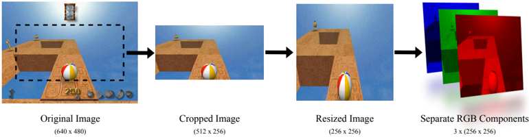The contents of the tuple are: - visual : an RGB array derived using the process shown in Figure 5. - reward : the value of instantaneous reward resulting from the move that has just been executed. - playing : a value indicating whether the player is still 'alive'. - clock : the number of seconds that remain in which the player must complete the level. - sound : one of either: None , if the practitioner has not instructed the abstraction to record the sound of moves; an array of Mel-frequency Cepstral Coefficients (MFCCs), if the abstraction was instantiated with use\_mfcc set to True ; or an array describing the raw audio output of the console over the duration of the move, otherwise. - duration\_real : the amount of time the move took to complete. - duration\_game : the amount of the player's remaining time that the move took to complete, relative to the in-game clock. - score : the score that the player has achieved so far in the current episode . When a move does not make a sound, sound will be an empty array. When a move makes a sound with a duration shorter than that of the move, silence from the recording will be removed from both its start and end. If a move's sound lasts longer than the duration of the move, the game will continue running until either the audio has ceased or the maximum recording time has been exceeded. The result of these features is that the audio output of moves is succinct, as shown in Appendix B, but that moves may take longer to execute when the abstraction is recording audio. Figure 5: Frame processing used for complex state representations. Images have their red, green and blue (RGB) channels separated. <details> <summary>Image 6 Details</summary>  ### Visual Description \n ## Diagram: Image Processing Steps ### Overview This diagram illustrates a sequence of image processing steps applied to an original image. The steps include cropping, resizing, and separating the image into its Red, Green, and Blue (RGB) color components. The diagram shows the visual result of each step. ### Components/Axes The diagram consists of four panels, arranged horizontally from left to right. Each panel is labeled with the name of the processing step and the resulting image dimensions. * **Original Image:** (640 x 480) * **Cropped Image:** (512 x 256) * **Resized Image:** (256 x 256) * **Separate RGB Components:** 3 x (256 x 256) The original image contains a beach scene with a ball, a small structure, and a dashed rectangle indicating the cropping area. A number "240" is visible in the bottom-left corner of the original image. ### Detailed Analysis or Content Details 1. **Original Image:** The image depicts a beach scene with a blue sky and water. A striped beach ball is prominently featured. A small, yellow structure is visible in the upper portion of the image. A dashed white rectangle outlines the area that will be cropped in the next step. The number "240" is present in the bottom-left corner. 2. **Cropped Image:** This image shows the portion of the original image within the dashed rectangle. The dimensions are 512 x 256 pixels. The beach ball and the yellow structure are still visible. 3. **Resized Image:** The cropped image has been resized to 256 x 256 pixels. The beach ball is now more centrally located. 4. **Separate RGB Components:** This panel displays three separate images, each representing one of the RGB color channels. * **Red Component:** Shows the image with only red color information. The beach ball appears as a bright area. * **Green Component:** Shows the image with only green color information. The beach and some parts of the ball are visible. * **Blue Component:** Shows the image with only blue color information. The sky and water are visible. ### Key Observations * The cropping step reduces the image size from 640x480 to 512x256. * The resizing step further reduces the image size to 256x256. * Separating the image into RGB components allows for individual analysis of each color channel. * The number "240" in the original image is not present in the subsequent images, suggesting it was within the cropped area. ### Interpretation This diagram demonstrates a basic image processing pipeline. The steps shown are common preprocessing techniques used in computer vision and image analysis. Cropping isolates a region of interest, resizing reduces computational complexity, and separating into RGB components allows for color-based analysis or manipulation. The diagram effectively illustrates how an image can be transformed through these operations. The presence of the number "240" in the original image, and its subsequent disappearance, suggests it was a metadata element or annotation that was removed during the cropping process. 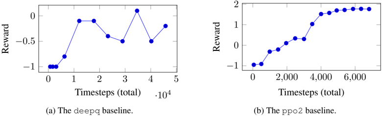</details> ## 6 Evaluation Appendix A gives example usage of both the game abstraction and the OpenAI Gym interface. The Kula-v1 Gym environment supports Kula World levels from 1 up to 10, uses the console's screen as its state encoding and (by default) uses the reward function described in Table 1. This environment was used with deepq and ppo2 from OpenAI Baselines 2 . The ppo2 baseline is an implementation of Proximal Policy Optimization Algorithms from Schulman et al. [17]. The results of these are shown in Figures 8a and 8b. 2 Available at https://github.com/openai/baselines Table 1: Reward function. | Event | Score change | Reward | |---------------|----------------|----------| | Coin collect | +250 | 0.2 | | Key collect | +1000 | 0.4 | | Fruit collect | +2500 | 0.6 | | Win level | - | 1 | | Lose level | - | -1 | <details> <summary>Image 7 Details</summary>  ### Visual Description \n ## Image: Collection of Game Screenshots ### Overview The image presents a 3x4 grid of screenshots, seemingly from a 3D computer game. Each screenshot depicts a different level or scene within the game, featuring a spherical character (a ball) navigating a complex, geometrically-structured environment. The environments appear to be desert-themed with various obstacles and structures. There is no explicit data or chart-like information present; it's a visual collection of game scenes. ### Components/Axes There are no axes, legends, or scales present in the image. The components are the individual screenshots themselves, each representing a distinct game level. Each screenshot contains: * A spherical character (ball) with varying color schemes (green/white, blue/white, red/white, yellow/white, purple/white, pink/white). * A geometrically complex environment constructed from blocks, platforms, and structures. * Background elements suggesting a desert landscape, including sand, rock formations, and water features. * Various obstacles and interactive elements within the levels. ### Detailed Analysis or Content Details The screenshots show the following: * **Row 1, Column 1:** Green and white ball on a tan platform with a building in the background. * **Row 1, Column 2:** Blue and white ball on a tan platform with a blue water feature and a pyramid-like structure. * **Row 1, Column 3:** Purple and white ball on a tan platform with a red structure resembling a tower. * **Row 1, Column 4:** Red and white ball on a tan platform with a blue water feature and a tall, thin structure. * **Row 2, Column 1:** Green and white ball on a tan platform with a building and a ramp. * **Row 2, Column 2:** Yellow and white ball on a tan platform with a hole and a ramp. * **Row 2, Column 3:** Beige ball on a tan platform with a maze-like structure. * **Row 2, Column 4:** Pink and white ball on a tan platform with a red and black structure. * **Row 3, Column 1:** Purple and white ball on a tan platform with a complex structure. * **Row 3, Column 2:** Blue and white ball on a tan platform with a blue water feature and a bridge. * **Row 3, Column 3:** Yellow and white ball on a tan platform with a desert background. * **Row 3, Column 4:** Blue and white ball on a tan platform with a structure. ### Key Observations The game appears to focus on navigating a spherical character through challenging, geometrically-designed levels. The color of the ball varies between screenshots, potentially indicating different characters or stages. The environments are consistently desert-themed, but with varying structures and obstacles. There is no numerical data or quantifiable information present. ### Interpretation The image showcases a 3D puzzle or platforming game. The levels are designed to test the player's spatial reasoning and problem-solving skills. The varying ball colors might represent different playable characters with unique abilities, or simply different levels of difficulty. The consistent desert theme suggests a unified setting for the game. The screenshots demonstrate a variety of level designs, indicating a potentially large and diverse game world. The lack of a user interface or score display in the screenshots suggests that the game focuses on the core gameplay experience of navigation and puzzle-solving rather than competitive scoring. The game appears to be visually simple, with a focus on geometric shapes and basic textures. It is difficult to determine the game's mechanics or objectives without further information. </details> (a) Starting locations, as used in training. (b) The evaluation episode start location. <details> <summary>Image 8 Details</summary>  ### Visual Description \n ## Screenshot: Marble Madness-Style Game Level ### Overview The image depicts a screenshot from a 3D computer game, reminiscent of the classic "Marble Madness". The scene shows a game level constructed from textured platforms, with a marble in motion. The overall aesthetic is stylized and somewhat dated, suggesting an older game. There is no chart or diagram to analyze, but rather a visual representation of a game environment. ### Components/Axes There are no axes or legends in this image. The visible components include: * **Platforms:** Two main platforms are visible, separated by a chasm. They are textured to resemble stone or wood with carved patterns. * **Marble:** A spherical object with red and white stripes, representing the player-controlled marble. * **Obstacles:** Various obstacles are present on the platforms, including a small tower, a triangular hole, a red "X" shaped barrier, and a circular hole. * **Collectibles:** Several collectible items are scattered around the platforms, including coins, bananas, and other unidentified objects. * **Hourglass:** An hourglass is positioned above the chasm, likely representing a time limit. * **Score Display:** A numerical display at the bottom center of the screen shows a score of "1000". * **Control Icon:** A small icon resembling a joystick or control pad is located in the bottom-left corner. ### Detailed Analysis or Content Details The scene is viewed from a slightly elevated perspective. The marble is positioned in the center of the image, appearing to be in motion. The platforms are decorated with carved patterns. The collectibles are scattered around the platforms, presumably to be collected by the marble. The hourglass suggests a time constraint for completing the level. The score display indicates the player's current score. * **Platform 1 (Left):** Contains a triangular hole, a red "X" shaped barrier, and a tower. * **Platform 2 (Right):** Contains a circular hole. * **Collectibles:** There are approximately 6-8 visible collectibles, including: * 3 gold coins * 2 grey objects (shape unclear) * 2 bananas * 1 yellow object (shape unclear) ### Key Observations The game appears to be focused on navigating a marble through a complex level, avoiding obstacles, and collecting items within a time limit. The visual style is reminiscent of early 3D games. The presence of an hourglass and a score display suggests a competitive element. ### Interpretation The image represents a level from a skill-based game where the player controls a marble. The objective is likely to navigate the marble through the level, avoiding obstacles and collecting items to earn points. The time limit adds a sense of urgency and challenge. The game's design suggests a focus on precision and timing. The overall aesthetic evokes a sense of nostalgia for classic arcade games. The level design appears to be intentionally challenging, requiring the player to carefully control the marble's movement. The scattered collectibles encourage exploration and reward skillful play. The image does not provide any factual data beyond the score of 1000. It is a visual representation of a game environment and its core gameplay elements. 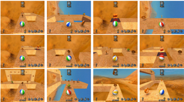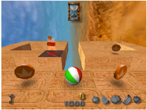</details> Figure 6: Screenshots from Kula World showing each possible start position. This approach to training is not particularly interesting, since the agent is presented with the same situation in each episode. As a result, the agent simply learns a set of moves which will result in it winning that level in the shortest time and with the highest score. To make the problem more challenging, we propose varying the player's start position within the level and the use of multiple levels. The game does not offer this feature by default, but it can be implemented using the tools available in PSXLE. To add an additional starting position for a player, simply save a PSXLE state with it at the desired position. We chose to limit the time available to complete each level to 80 seconds, rather than the usual 100, so that each starting state allowed the same amount of time to complete the level. The environment Kula-random-v1 takes this approach. It presents the agent with one of four different starting position in each of the first three levels of the game. There is an additional starting position within Level 2 that is reserved for use in validation episodes in which no learning takes place and the agent picks moves from its learned policy. Each of the starting positions are shown in Figure 6. 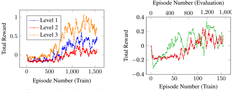We implemented a simple DQN agent based on the network presented in Mnih et al. [9], for use with Kula-random-v1 . The results are summarised in Figure 7a and Figure 7b. Surprisingly, the agent was most successful in learning how to play Level 3, despite it being the most complex for human players. This may be due to Level 3 introducing new physics that are not intuitive to humans, but are easier to navigate for the agent. Level 2 requires players jump between islands, meaning a jump can either be very profitable for a player (in that it gains access to more coins) or very bad (because the player falls off the platform). This discrepancy means that agents must disambiguate a jump that is required for it to reach the goal square from one that will end the game. By comparison, Level 3 does not require any jumps to complete. The agent performs similarly from the reserved start position as it did from the other available locations in Level 2. It is promising that the agent did not perform notably worse when given an unseen start state, it is also worth noting that the performance of the agent was fairly lacklustre on Level 2 in general. 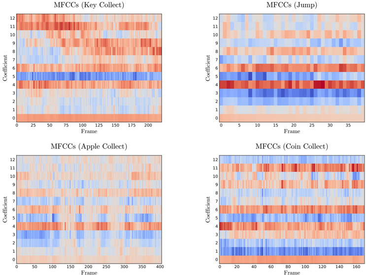In order to leverage the audio recording features of PSXLE, we developed another environment: Kula-audio-v1 . This environment includes a representation of the audio output from each move within its state encoding. The state encoding is the richest yet, containing visual output, audio output, time remaining on the level and score. Since MFCCs have been successful in machine learning contexts for classifying audio data, they are used here to represent the audio output of a move. The MFCC outputs for some moves are shown in Appendix B. Finally, since the agent starts each episode from a specified state, the states in its memory are dominated by those that occur at the start of the level. For PlayStation games, which are usually quite complex and have long levels, this can result in lenghtly training times. Prioritised experience replay [6] attempts to combat this by replaying state transitions that the agent learned the most from. We propose a modification to this, prioritised state replay , in which an agent can resume play from a state which it has previously visited, allowing the agent to perform a different action. This can be trivially implemented using the save\_state and load\_state methods in PSXLE and could help to reduce the time required to learn complex games. No agents have been trained using this approach. <details> <summary>Image 9 Details</summary>  ### Visual Description ## Line Chart: Training and Evaluation Reward Curves ### Overview The image presents two line charts displaying the total reward obtained during training and evaluation across three levels. The left chart shows the reward during the training phase, while the right chart shows the reward during the evaluation phase. Both charts use episode number as the independent variable and total reward as the dependent variable. ### Components/Axes * **Left Chart:** * X-axis: "Episode Number (Train)" ranging from 0 to 1500, with tick marks at 0, 500, 1000, and 1500. * Y-axis: "Total Reward" ranging from -0.2 to 1.0, with tick marks at 0, 0.2, 0.4, 0.6, 0.8, and 1.0. * Legend: Located in the top-left corner, with labels "Level 1" (blue line), "Level 2" (red line), and "Level 3" (orange line). * **Right Chart:** * X-axis: "Episode Number (Train)" ranging from 0 to 150, with tick marks at 0, 50, 100, and 150. * Y-axis: "Total Reward" ranging from -0.4 to 0.4, with tick marks at -0.4, -0.2, 0, 0.2, and 0.4. * Legend: No explicit legend is present, but the lines are colored as follows: green, red, and blue. * **Header:** "Episode Number (Evaluation)" with tick marks at 0, 400, 800, 1200, and 1600. This is positioned above the right chart. ### Detailed Analysis or Content Details * **Left Chart (Training Reward):** * **Level 1 (Blue):** Starts around -0.1 at episode 0, increases gradually to approximately 0.5 around episode 500, fluctuates between 0.3 and 0.7, and reaches a maximum of approximately 0.8 around episode 1300, finishing at approximately 0.5. * **Level 2 (Red):** Starts around -0.1 at episode 0, increases to approximately 0.3 around episode 500, fluctuates between 0.1 and 0.5, and reaches a maximum of approximately 0.6 around episode 1200, finishing at approximately 0.2. * **Level 3 (Orange):** Starts around -0.1 at episode 0, increases to approximately 0.4 around episode 500, fluctuates between 0.2 and 0.8, and reaches a maximum of approximately 0.9 around episode 1000, finishing at approximately 0.3. * **Right Chart (Evaluation Reward):** * **Green Line:** Starts around 0.1 at episode 0, increases to approximately 0.25 around episode 50, fluctuates between 0 and 0.3, and finishes at approximately 0.2. * **Red Line:** Starts around 0 at episode 0, decreases to approximately -0.2 around episode 20, fluctuates between -0.3 and 0.1, and finishes at approximately -0.1. * **Blue Line:** Starts around 0 at episode 0, decreases to approximately -0.3 around episode 20, fluctuates between -0.4 and 0, and finishes at approximately -0.2. ### Key Observations * The training reward (left chart) generally increases with the episode number for all levels, indicating learning progress. Level 3 consistently achieves the highest reward during training. * The evaluation reward (right chart) shows more variability and generally lower rewards compared to the training reward. * Level 2 and Level 3 show a negative reward during the initial evaluation episodes. * The evaluation reward for Level 1 (green line) is consistently positive, while the evaluation rewards for Level 2 (red line) and Level 3 (blue line) are mostly negative. ### Interpretation The charts demonstrate the learning process of an agent across three levels of complexity. The increasing training rewards suggest that the agent is improving its performance as it interacts with the environment. However, the evaluation rewards indicate a potential gap between training and generalization performance. The negative evaluation rewards for Levels 2 and 3 suggest that the agent may be overfitting to the training environment or struggling to adapt to unseen scenarios. The consistent positive evaluation reward for Level 1 suggests that the agent is able to generalize well to new situations in this level. The difference between the training and evaluation rewards highlights the importance of evaluating the agent's performance on a separate dataset to assess its true capabilities. The higher rewards achieved by Level 3 during training suggest that it is the most challenging level, but also the one where the agent has the greatest potential for improvement. </details> - (b) The green line shows a moving average over 5 validation episodes for the reserved location, the red line is the same as in Figure 7a. - (a) Agent proficiency on each level during training. Start locations within each level are chosen uniformly at random from those shown in Figure 6. The line shows a moving average over 10 training episodes. Figure 7: Evaluation of a simple DQN implementation for Kula-random-v1 . <details> <summary>Image 10 Details</summary>  ### Visual Description \n ## Line Chart: Reward vs. Timesteps for Baseline Algorithms ### Overview The image presents two line charts comparing the reward achieved by two reinforcement learning algorithms, `deepq` and `ppo2`, over time (measured in timesteps). Both charts plot Reward (y-axis) against Timesteps (total) (x-axis). ### Components/Axes * **Chart 1 (Left):** * **Title:** (a) The deepq baseline. * **X-axis Label:** Timesteps (total) * **X-axis Scale:** 0 to 5, with a secondary scale indicating `.10^4` at the end. * **Y-axis Label:** Reward * **Y-axis Scale:** -1 to 0. * **Chart 2 (Right):** * **Title:** (b) The ppo2 baseline. * **X-axis Label:** Timesteps (total) * **X-axis Scale:** 0 to 6,000. * **Y-axis Label:** Reward * **Y-axis Scale:** -1 to 2. * **Data Series:** Both charts have a single data series represented by blue circles connected by a blue line. ### Detailed Analysis or Content Details **Chart 1: deepq baseline** The line representing the `deepq` baseline shows a fluctuating reward pattern. The line initially slopes upward, then fluctuates. * Timestep 0: Reward ≈ -0.95 * Timestep 0.5: Reward ≈ -0.8 * Timestep 1: Reward ≈ -0.3 * Timestep 2: Reward ≈ -0.6 * Timestep 3: Reward ≈ 0.2 * Timestep 4: Reward ≈ -0.5 * Timestep 5: Reward ≈ -0.2 **Chart 2: ppo2 baseline** The line representing the `ppo2` baseline shows a consistently increasing reward pattern. The line slopes upward throughout the entire duration. * Timestep 0: Reward ≈ -1.0 * Timestep 1,000: Reward ≈ -0.2 * Timestep 2,000: Reward ≈ 0.2 * Timestep 3,000: Reward ≈ 0.8 * Timestep 4,000: Reward ≈ 1.4 * Timestep 5,000: Reward ≈ 1.8 * Timestep 6,000: Reward ≈ 1.9 ### Key Observations * The `ppo2` baseline consistently achieves higher rewards than the `deepq` baseline. * The `deepq` baseline exhibits significant fluctuations in reward, indicating instability in the learning process. * The `ppo2` baseline demonstrates a clear upward trend, suggesting stable and effective learning. * The `deepq` baseline appears to plateau at a lower reward level. ### Interpretation The data suggests that the `ppo2` algorithm is more effective at learning the task than the `deepq` algorithm, as evidenced by its consistently higher and increasing reward. The fluctuations observed in the `deepq` baseline may indicate sensitivity to hyperparameters or the stochastic nature of the environment. The consistent upward trend of the `ppo2` baseline suggests a more robust and stable learning process. The difference in performance highlights the importance of algorithm selection in reinforcement learning tasks. The `deepq` baseline's performance is relatively low and unstable, while the `ppo2` baseline demonstrates a clear ability to learn and improve over time. This comparison provides valuable insights into the strengths and weaknesses of each algorithm in this specific context. </details> Figure 8: A plot of the average reward over 100 episodes, as given by OpenAI Baselines, against the number of timesteps that the agent had played. The agents were trained on Level 1 of Kula World using a visual state encoding. ## 7 Conclusion The results from deepq and ppo2 baselines show how two different RL algorithms can perform to a vastly different standard within the Kula World environment. From this, it is clear that PlayStation games can represent suitable environments in which to evaluate the effectiveness of RL algorithms. The approach shown in this paper for Kula World can be customised to work with many different PlayStation games. The design of PSXLE makes it simple to build abstractions that support interfaces like OpenAI Gym. Armed with such abstractions, researchers will be able to apply existing RL implementations on more complex environments with richer state spaces. The challenges that the audio and complex visual rendering in PlayStation games present to RL could help us to close the gap between what we want agents to achieve and the methodology that we use to evaluate them. ## Appendices ## A Library usage To demonstrate the functionality of the work presented in this paper, example scripts are shown below. These are chosen to show how practitioners can interact with the environment at each level of abstraction. ## A.1 Console This script creates a console running Kula World, loads Level 1 and moves the player forwards two steps. ``` ``` ## A.2 Game abstraction This script creates a Game object for Kula World and plays it randomly. ``` ``` ## A.3 Interface This script uses the OpenAI Gym implementation of Kula World to play randomly. Note that the methods being used are entirely game-agnostic. 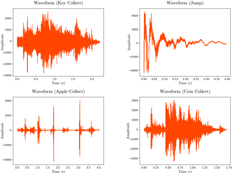``` ``` ``` ``` ## B Audio outputs Figure 9: Raw audio output for a selection of moves within Kula World, obtained using PSXLE's audio recording feature. The abstraction employs cropping and extended move times to ensure that the full audio waveform for each move is captured. <details> <summary>Image 11 Details</summary>  ### Visual Description \n ## Charts: Waveform Analysis - Sound Event Detection ### Overview The image presents four separate waveform plots, each representing the amplitude of a sound signal over time. Each plot is labeled with the type of sound event it depicts: "Key Collect", "Jump", "Apple Collect", and "Coin Collect". The plots are arranged in a 2x2 grid. The y-axis represents Amplitude, and the x-axis represents Time (in seconds). ### Components/Axes * **X-axis:** Time (s) - Ranges vary per plot. * **Y-axis:** Amplitude - Ranges vary per plot, approximately from -4000 to 4000. * **Titles:** Each plot has a title indicating the sound event: "Waveform (Key Collect)", "Waveform (Jump)", "Waveform (Apple Collect)", "Waveform (Coin Collect)". * **Data Series:** Each plot contains a single orange line representing the waveform. ### Detailed Analysis or Content Details **1. Waveform (Key Collect):** * **Time Range:** 0.0 to 2.2 seconds. * **Trend:** The waveform is highly variable, exhibiting numerous peaks and troughs. It appears to be a relatively noisy signal with no clear repeating pattern. * **Amplitude:** Fluctuates rapidly between approximately -3000 and 3000. * **Notable Points:** Multiple peaks around 0.2s, 0.7s, 1.3s, 1.8s, with amplitudes around 2000-3000. Multiple troughs around 0.5s, 1.0s, 1.6s, 2.0s, with amplitudes around -2000 to -3000. **2. Waveform (Jump):** * **Time Range:** 0.0 to 0.4 seconds. * **Trend:** The waveform starts with a large positive spike, followed by a rapid decay and then smaller oscillations. * **Amplitude:** Initial spike reaches approximately 4000, then decays to around 1000-2000. * **Notable Points:** A large peak at approximately 0.02 seconds with an amplitude of around 4000. The signal then quickly drops to around 1000-2000 and oscillates around that level. **3. Waveform (Apple Collect):** * **Time Range:** 0.0 to 4.2 seconds. * **Trend:** The waveform consists of several distinct, relatively sharp peaks separated by periods of lower amplitude. The peaks are somewhat periodic. * **Amplitude:** Peaks reach approximately 3000-4000, troughs reach approximately -4000. * **Notable Points:** Peaks are observed around 0.3s, 1.0s, 1.8s, 2.6s, 3.4s, with amplitudes around 3000. Troughs are observed between the peaks. **4. Waveform (Coin Collect):** * **Time Range:** 0.0 to 1.75 seconds. * **Trend:** The waveform exhibits a series of closely spaced, high-frequency oscillations, followed by a more gradual decay. * **Amplitude:** Oscillations range from approximately -3000 to 3000. * **Notable Points:** A dense series of peaks and troughs within the first 0.75 seconds. The amplitude then decreases. ### Key Observations * The "Jump" waveform has a very distinct initial spike, unlike the others. * The "Apple Collect" waveform shows a more periodic pattern of peaks than the "Key Collect" waveform. * The "Coin Collect" waveform has the highest frequency of oscillations. * The "Key Collect" waveform appears to be the most chaotic and least structured. ### Interpretation These waveforms likely represent audio recordings of the corresponding sound events. The differences in the waveforms reflect the distinct acoustic characteristics of each event. The "Jump" waveform's sharp initial spike suggests a sudden impact or change in sound pressure. The "Apple Collect" waveform's periodic peaks could be related to the repetitive nature of collecting apples (e.g., the sound of each apple being picked up). The "Coin Collect" waveform's high-frequency oscillations are characteristic of metallic impacts. The "Key Collect" waveform's complexity suggests a more varied and less predictable sound. These waveforms could be used for sound event detection or classification tasks. Analyzing the features of these waveforms (e.g., peak amplitude, frequency content, temporal patterns) could allow a machine learning model to identify and categorize these sounds automatically. The differences in the waveforms suggest that these events are readily distinguishable based on their acoustic properties. </details> Figure 10: MFCCs derived from the waveforms in Figure 9. <details> <summary>Image 12 Details</summary>  ### Visual Description ## Heatmaps: MFCCs Coefficient Variation Across Frames ### Overview The image presents four heatmaps, each visualizing the variation of MFCCs (Mel-Frequency Cepstral Coefficients) across different frames for four distinct actions: "Key Collect", "Jump", "Apple Collect", and "Coin Collect". The heatmaps display the coefficient value (ranging from approximately 0 to 12) on the y-axis against the frame number on the x-axis. Color intensity represents the coefficient value, with red indicating higher values and blue indicating lower values. ### Components/Axes Each heatmap shares the following components: * **X-axis:** "Frame" - Represents the frame number in the video sequence. The scales vary for each action: * "Key Collect": 0 to 200 * "Jump": 0 to 35 * "Apple Collect": 0 to 400 * "Coin Collect": 0 to 160 * **Y-axis:** "Coefficient" - Represents the MFCC coefficient number, ranging from 0 to 12. * **Color Scale:** A diverging color scale where red represents high coefficient values, blue represents low coefficient values, and white/light shades represent values near zero. * **Titles:** Each heatmap has a title indicating the action being analyzed (e.g., "MFCCs (Key Collect)"). ### Detailed Analysis or Content Details **1. MFCCs (Key Collect)** * The heatmap spans frames 0 to 200 and coefficients 0 to 12. * The overall trend shows a dynamic pattern of coefficient variation. * Initially (frames 0-25), coefficients 6-12 exhibit relatively high values (approximately 8-12, indicated by red color). * From frames 25-75, there's a transition with coefficients 0-5 increasing in value while the higher coefficients decrease. * Between frames 75-150, the pattern becomes more complex, with fluctuating values across all coefficients. * From frames 150-200, coefficients 0-5 show a decrease in value, while coefficients 6-12 increase again. **2. MFCCs (Jump)** * The heatmap spans frames 0 to 35 and coefficients 0 to 12. * The initial frames (0-10) show relatively low coefficient values (approximately 0-4, indicated by blue color). * A rapid increase in coefficient values (6-12) occurs between frames 10-20, peaking around a value of 10-12 (red color). * From frames 20-35, the coefficients gradually decrease, returning to lower values. **3. MFCCs (Apple Collect)** * The heatmap spans frames 0 to 400 and coefficients 0 to 12. * The initial frames (0-50) show a relatively stable pattern with coefficients 6-12 having moderate values (approximately 4-8). * From frames 50-200, there's a significant increase in coefficient variation, with fluctuating values across all coefficients. * Between frames 200-300, the pattern stabilizes again, with coefficients 0-5 showing higher values (approximately 6-10). * From frames 300-400, the coefficients gradually decrease. **4. MFCCs (Coin Collect)** * The heatmap spans frames 0 to 160 and coefficients 0 to 12. * The initial frames (0-20) show low coefficient values (approximately 0-4, indicated by blue color). * A rapid increase in coefficient values (6-12) occurs between frames 20-60, peaking around a value of 8-12 (red color). * From frames 60-120, the coefficients fluctuate with moderate values. * Between frames 120-160, the coefficients gradually decrease. ### Key Observations * The "Jump" action exhibits the most distinct and rapid change in MFCC coefficients, with a clear peak around frames 10-20. * "Key Collect" and "Apple Collect" show more gradual and complex variations in coefficients over longer frame durations. * "Coin Collect" shows a similar pattern to "Jump" but with a slightly slower and more sustained increase in coefficients. * The higher-order coefficients (6-12) generally exhibit greater variation than the lower-order coefficients (0-5). ### Interpretation These heatmaps demonstrate how MFCCs, which represent the spectral envelope of a sound, change over time during different actions. The variations in coefficients reflect the dynamic characteristics of the sounds associated with each action. The distinct patterns observed for each action suggest that MFCCs can be used as features for action recognition. The rapid change in coefficients during the "Jump" action likely corresponds to the impact sound and the associated changes in vocalization or body movement. The more gradual changes in "Key Collect" and "Apple Collect" may reflect the continuous nature of these actions and the subtle variations in sounds produced during their execution. The differences in the heatmap patterns highlight the potential for using machine learning algorithms to classify actions based on their MFCC profiles. The outliers and trends observed in the data can provide insights into the specific acoustic features that are most discriminative for each action. The varying frame lengths suggest that the duration of each action differs, which could also be a useful feature for classification. </details> ## References - [1] S. Wang, D. Jia, and X. Weng, 'Deep Reinforcement Learning for Autonomous Driving,' arXiv e-prints , p. arXiv:1811.11329, Nov 2018. - [2] I. Arel, C. Liu, T. Urbanik, and A. G. Kohls, 'Reinforcement learning-based multi-agent system for network traffic signal control,' IET Intelligent Transport Systems , vol. 4, pp. 128-135, June 2010. - [3] J. Jin, C. Song, H. Li, K. Gai, J. Wang, and W. Zhang, 'Real-Time Bidding with Multi-Agent Reinforcement Learning in Display Advertising,' arXiv e-prints , p. arXiv:1802.09756, Feb 2018. - [4] S. Levine, C. Finn, T. Darrell, and P. Abbeel, 'End-to-End Training of Deep Visuomotor Policies,' arXiv e-prints , p. arXiv:1504.00702, Apr 2015. - [5] H. van Hasselt, A. Guez, and D. Silver, 'Deep Reinforcement Learning with Double Q-Learning,' AAAI Conference on Artificial Intelligence , 2016. - [6] T. Schaul, J. Quan, I. Antonoglou, and D. Silver, 'Prioritized Experience Replay,' arXiv e-prints , p. arXiv:1511.05952, Nov 2015. - [7] Z. Wang, T. Schaul, M. Hessel, H. Hasselt, M. Lanctot, and N. Freitas, 'Dueling Network Architectures for Deep Reinforcement Learning,' Proceedings of The 33rd International Conference on Machine Learning , vol. 48, pp. 1995-2003, 20-22 Jun 2016. - [8] V. Mnih, A. P. Badia, M. Mirza, A. Graves, T. Lillicrap, T. Harley, D. Silver, and K. Kavukcuoglu, 'Asynchronous Methods for Deep Reinforcement Learning,' Proceedings of The 33rd International Conference on Machine Learning , vol. 48, pp. 1928-1937, 20-22 Jun 2016. - [9] V. Mnih, K. Kavukcuoglu, D. Silver, A. A. Rusu, J. Veness, M. G. Bellemare, A. Graves, M. Riedmiller, A. K. Fidjeland, G. Ostrovski, S. Petersen, C. Beattie, A. Sadik, I. Antonoglou, H. King, D. Kumaran, D. Wierstra, S. Legg, and D. Hassabis, 'Human-level control through deep reinforcement learning,' Nature , vol. 518, pp. 529 EP -, Feb 2015. - [10] G. Brockman and J. Schulman, 'OpenAI Gym Beta.' https://openai.com/blog/ openai-gym-beta/ . Accessed: 2019-01-12. - [11] D. T. Behrens, 'Deep Reinforcement Learning and Autonomous Driving.' https:// ai-guru.de/deep-reinforcement-learning-and-autonomous-driving/ . Accessed: 2019-03-04. - [12] OpenAI, 'OpenAI Gym Environments.' https://gym.openai.com/envs/ . Accessed: 2019-01-12. - [13] M. G. Bellemare, Y. Naddaf, J. Veness, and M. Bowling, 'The Arcade Learning Environment: An Evaluation Platform for General Agents,' arXiv e-prints , p. arXiv:1207.4708, Jul 2012. - [14] G. Hinton, L. Deng, D. Yu, G. E. Dahl, A. Mohamed, N. Jaitly, A. Senior, V. Vanhoucke, P. Nguyen, T. N. Sainath, and B. Kingsbury, 'Deep Neural Networks for Acoustic Modeling in Speech Recognition: The Shared Views of Four Research Groups,' IEEE Signal Processing Magazine , vol. 29, pp. 82-97, Nov 2012. - [15] Z. Zeng, J. Tu, B. M. Pianfetti, and T. S. Huang, 'Audio-Visual Affective Expression Recognition Through Multistream Fused HMM,' IEEE Transactions on Multimedia , vol. 10, pp. 570577, June 2008. - [16] Xi Shao, Changsheng Xu, and M. S. Kankanhalli, 'Unsupervised classification of music genre using hidden Markov model,' in 2004 IEEE International Conference on Multimedia and Expo (ICME) (IEEE Cat. No.04TH8763) , vol. 3, pp. 2023-2026 Vol.3, June 2004. - [17] J. Schulman, F. Wolski, P. Dhariwal, A. Radford, and O. Klimov, 'Proximal Policy Optimization Algorithms,' arXiv e-prints , p. arXiv:1707.06347, Jul 2017.