2005.00341v1

# Jukebox: A Generative Model for Music **Authors**: Prafulla Dhariwal, Heewoo Jun, Christine Payne, Jong Wook Kim, Alec Radford, Ilya Sutskever ## Jukebox: A Generative Model for Music Prafulla Dhariwal * 1 Heewoo Jun * 1 Christine Payne * 1 Jong Wook Kim 1 Alec Radford 1 Ilya Sutskever 1 ## Abstract We introduce Jukebox, a model that generates music with singing in the raw audio domain. We tackle the long context of raw audio using a multiscale VQ-VAE to compress it to discrete codes, and modeling those using autoregressive Transformers. We show that the combined model at scale can generate high-fidelity and diverse songs with coherence up to multiple minutes. We can condition on artist and genre to steer the musical and vocal style, and on unaligned lyrics to make the singing more controllable. We are releasing thousands of non cherry-picked samples, along with model weights and code. ## 1. Introduction Music is an integral part of human culture, existing from the earliest periods of human civilization and evolving into a wide diversity of forms. It evokes a unique human spirit in its creation, and the question of whether computers can ever capture this creative process has fascinated computer scientists for decades. We have had algorithms generating piano sheet music (Hiller Jr & Isaacson, 1957; Moorer, 1972; Hadjeres et al., 2017; Huang et al., 2017), digital vocoders generating a singer's voice (Bonada & Serra, 2007; Saino et al., 2006; Blaauw & Bonada, 2017) and also synthesizers producing timbres for various musical instruments (Engel et al., 2017; 2019). Each captures a specific aspect of music generation: melody, composition, timbre, and the human voice singing. However, a single system to do it all remains elusive. The field of generative models has made tremendous progress in the last few years. One of the aims of generative modeling is to capture the salient aspects of the data and to generate new instances indistinguishable from the true data The hypothesis is that by learning to produce the data we can learn the best features of the data 1 . We are surrounded by highly complex distributions in the visual, audio, and text domain, and in recent years we have devel- * Equal contribution 1 OpenAI, San Francisco. Correspondence to: <jukebox@openai.com>. oped advances in text generation (Radford et al.), speech generation (Xie et al., 2017) and image generation (Brock et al., 2019; Razavi et al., 2019). The rate of progress in this field has been rapid, where only a few years ago we had algorithms producing blurry faces (Kingma & Welling, 2014; Goodfellow et al., 2014) but now we now can generate high-resolution faces indistinguishable from real ones (Zhang et al., 2019b). Generative models have been applied to the music generation task too. Earlier models generated music symbolically in the form of a pianoroll, which specifies the timing, pitch, velocity, and instrument of each note to be played. (Yang et al., 2017; Dong et al., 2018; Huang et al., 2019a; Payne, 2019; Roberts et al., 2018; Wu et al., 2019). The symbolic approach makes the modeling problem easier by working on the problem in the lower-dimensional space. However, it constrains the music that can be generated to being a specific sequence of notes and a fixed set of instruments to render with. In parallel, researchers have been pursuing the nonsymbolic approach, where they try to produce music directly as a piece of audio. This makes the problem more challenging, as the space of raw audio is extremely high dimensional with a high amount of information content to model. There has been some success, with models producing piano pieces either in the raw audio domain (Oord et al., 2016; Mehri et al., 2017; Yamamoto et al., 2020) or in the spectrogram domain (Vasquez & Lewis, 2019). The key bottleneck is that modeling the raw audio directly introduces extremely long-range dependencies, making it computationally challenging to learn the high-level semantics of music. A way to reduce the difficulty is to learn a lower-dimensional encoding of the audio with the goal of losing the less important information but retaining most of the musical information. This approach has demonstrated some success in generating short instrumental pieces restricted to a set of a few instruments (Oord et al., 2017; Dieleman et al., 2018). In this work, we show that we can use state-of-the-art deep generative models to produce a single system capable of generating diverse high-fidelity music in the raw audio domain, with long-range coherence spanning multiple minutes. Our approach uses a hierarchical VQ-VAE architecture (Razavi 1 Richard Feynmann famously said, 'What I cannot create, I do not understand' et al., 2019) to compress audio into a discrete space, with a loss function designed to retain the maximum amount of musical information, while doing so at increasing levels of compression. We use an autoregressive Sparse Transformer (Child et al., 2019; Vaswani et al., 2017) trained with maximum-likelihood estimation over this compressed space, and also train autoregressive upsamplers to recreate the lost information at each level of compression. We show that our models can produce songs from highly diverse genres of music like rock, hip-hop, and jazz. They can capture melody, rhythm, long-range composition, and timbres for a wide variety of instruments, as well as the styles and voices of singers to be produced with the music. We can also generate novel completions of existing songs. Our approach allows the option to influence the generation process: by swapping the top prior with a conditional prior, we can condition on lyrics to tell the singer what to sing, or on midi to control the composition. We release our model weights and training and sampling code at https://github.com/openai/jukebox. ## 2. Background We consider music in the raw audio domain represented as a continuous waveform x ∈ [ -1 , 1] T , where the number of samples T is the product of the audio duration and the sampling rate typically ranging from 16 kHz to 48 kHz. For music, CD quality audio, 44.1 kHz samples stored in 16 bit precision, is typically enough to capture the range of frequencies perceptible to humans. As an example, a fourminute-long audio segment will have an input length of ∼ 10 million, where each position can have 16 bits of information. In comparison, a high-resolution RGB image with 1024 × 1024 pixels has an input length of ∼ 3 million, and each position has 24 bits of information. This makes learning a generative model for music extremely computationally demanding with increasingly longer durations; we have to capture a wide range of musical structures from timbre to global coherence while simultaneously modeling a large amount of diversity. ## 2.1. 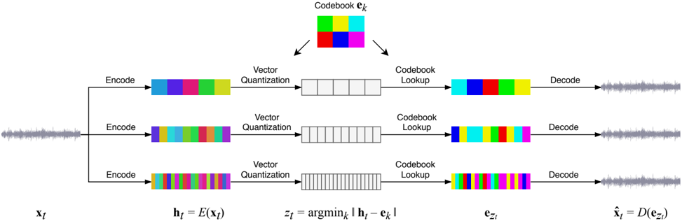VQ-VAE To make this task feasible, we use the VQ-V AE (Oord et al., 2017; Dieleman et al., 2018; Razavi et al., 2019) to compress raw audio to a lower-dimensional space. A one-dimensional VQ-VAE learns to encode an input sequence x = 〈 x t 〉 T t =1 using a sequence of discrete tokens z = 〈 z s ∈ [ K ] 〉 S s =1 , where K denotes the vocabulary size and we call the ratio T/S the hop length. It consists of an encoder E ( x ) which encodes x into a sequence of latent vectors h = 〈 h s 〉 S s =1 , a bottleneck that quantizes h s ↦→ e z s by mapping each h s to its nearest vector e z s from a codebook C = { e k } K k =1 , and a decoder D ( e ) that decodes the embedding vectors back to the input space. It is thus an auto-encoder with a discretization bottleneck. The VQ-VAE is trained using the following objective: $$\begin{aligned} & L = L _ { recons } + L _ { codeb } \\ & = \beta L _ { commit } ( 1 )$$ $$L _ { r e c o n s } = \frac { 1 } { t } \sum _ { t } ^ { L } || x _ { t } - D ( e _ { z } ) || ^ { 2 }$$ $$\sum _ { s } ^ { 1 } \sum _ { g } ^ { 1 } | S g | h$$ $$\sum _ { s = 1 } ^ { \infty } \sum _ { h = 1 } ^ { \infty } - g [ e _ { x _ { s } } ] ^ { 2 }$$ where sg denotes the stop-gradient operation, which passes zero gradient during backpropagation. The reconstruction loss L recons penalizes for the distance between the input x and the reconstructed output ̂ x = D ( e z ) , and L codebook penalizes the codebook for the distance between the encodings h and their nearest neighbors e z from the codebook. To stabilize the encoder, we also add L commit to prevent the encodings from fluctuating too much, where the weight β controls the amount of contribution of this loss. To speed up training, the codebook loss L codebook instead uses EMA updates over the codebook variables. Razavi et al. (2019) extends this to a hierarchical model where they train a single encoder and decoder but break up the latent sequence h into a multi-level representation [ h (1) , · · · , h ( L ) ] with decreasing sequence lengths, each learning its own codebook C ( l ) . They use non-autoregressive encoder-decoders and jointly train all levels with a simple mean-squared loss. ## 3. Music VQ-VAE Inspired by the results from the hierarchical VQ-V AE model (Razavi et al., 2019) for images, we consider applying the same technique to model raw audio using three different levels of abstraction, as illustrated in Figure 1. At each level, we use residual networks consisting of WaveNet-style noncausal 1-D dilated convolutions, interleaved with downsampling and upsampling 1-D convolutions to match different hop lengths. A detailed description of the architecture is provided in Appendix B.1. We make a number of modifications to our VQ-VAE compared to the ones in (Oord et al., 2017; Razavi et al., 2019), as described in the following subsections. ## 3.1. Random restarts for embeddings VQ-VAEs are known to suffer from codebook collapse, wherein all encodings get mapped to a single or few embedding vectors while the other embedding vectors in the codebook are not used, reducing the information capacity of the bottleneck. To prevent this, we use random restarts: when the mean usage of a codebook vector falls below a threshold, we randomly reset it to one of the encoder outputs from the current batch. This ensures all vectors in the Figure 1. We first train three separate VQ-V AE models with different temporal resolutions. At each level, the input audio is segmented and encoded into latent vectors h t , which are then quantized to the closest codebook vectors e z t . The code z t is a discrete representation of the audio that we later train our prior on. The decoder takes the sequence of codebook vectors and reconstructs the audio. The top level learns the highest degree of abstraction, since it is encoding longer audio per token while keeping the codebook size the same. Audio can be reconstructed using the codes at any one of the abstraction levels, where the least abstract bottom-level codes result in the highest-quality audio, as shown in Figure 4. For the detailed structure of each component, see Figure 7. <details> <summary>Image 1 Details</summary>  ### Visual Description ## Diagram: Multi-scale Vector Quantization Process ### Overview This diagram illustrates a multi-scale vector quantization (VQ) architecture, commonly used in signal processing (such as audio or image compression). The process takes an input signal ($x_t$) and processes it through three parallel branches of increasing resolution (coarse to fine). Each branch encodes the signal, quantizes it using a shared codebook ($e_k$), and subsequently decodes it to reconstruct the signal ($\hat{x}_t$). ### Components/Axes The diagram is organized into three horizontal processing branches, with a shared codebook component at the top center. * **Input/Output:** * **Left:** $x_t$ (Input signal waveform). * **Right:** $\hat{x}_t = D(e_{z_t})$ (Reconstructed output signal waveform). * **Mathematical Notations (Bottom Row):** * $h_t = E(x_t)$: The encoded representation of the input. * $z_t = \text{argmin}_k || h_t - e_k ||$: The quantization step, selecting the nearest codebook vector. * $e_{z_t}$: The quantized representation (the codebook vectors selected). * **Central Component:** * **Codebook $e_k$:** Located at the top-center, represented as a 2x3 grid of colored blocks (Yellow, Cyan, Red, Blue, Green, Magenta). * **Processing Steps (Left to Right):** * **Encode:** Transforms input into a latent representation. * **Vector Quantization:** A white box with vertical dividers representing the selection process. * **Codebook Lookup:** Maps the quantized index to the actual codebook vector. * **Decode:** Reconstructs the signal from the quantized vectors. ### Detailed Analysis The diagram is segmented into three parallel horizontal branches, representing different scales of quantization: 1. **Top Branch (Coarse Scale):** * **Encoded Representation ($h_t$):** Contains 5 distinct colored segments. * **Vector Quantization:** The white box contains 4 vertical dividers (creating 5 slots). * **Codebook Lookup ($e_{z_t}$):** Produces 5 colored segments, matching the input $h_t$ pattern. 2. **Middle Branch (Medium Scale):** * **Encoded Representation ($h_t$):** Contains 10 distinct colored segments. * **Vector Quantization:** The white box contains 9 vertical dividers (creating 10 slots). * **Codebook Lookup ($e_{z_t}$):** Produces 10 colored segments, matching the input $h_t$ pattern. 3. **Bottom Branch (Fine Scale):** * **Encoded Representation ($h_t$):** Contains 20 distinct colored segments. * **Vector Quantization:** The white box contains 19 vertical dividers (creating 20 slots). * **Codebook Lookup ($e_{z_t}$):** Produces 20 colored segments, matching the input $h_t$ pattern. ### Key Observations * **Resolution Scaling:** There is a clear progression in resolution. The top branch is the "coarsest" (lowest number of segments), while the bottom branch is the "finest" (highest number of segments). * **Shared Codebook:** The arrows originating from the "Codebook $e_k$" block point to all three "Vector Quantization" stages, indicating that the same codebook is utilized across all scales. * **Reconstruction Fidelity:** The output $\hat{x}_t$ on the right shows a waveform that visually resembles the input $x_t$ on the left, demonstrating the reconstruction capability of the system. * **Mathematical Logic:** The formula $z_t = \text{argmin}_k || h_t - e_k ||$ explicitly defines the quantization process as finding the codebook vector ($e_k$) that minimizes the Euclidean distance to the encoded input ($h_t$). ### Interpretation This diagram represents a **Residual Vector Quantization (RVQ)** or a **Multi-scale VQ** system. * **Functionality:** The system decomposes the input signal into hierarchical layers. The top layer captures the most significant, low-frequency, or "coarse" information, while the lower layers capture increasingly granular, high-frequency, or "fine" details. * **Efficiency:** By using a shared codebook ($e_k$) across different scales, the model can efficiently represent complex signals using a limited set of learned patterns. * **Process Flow:** The "Vector Quantization" block acts as a bottleneck or a decision point. It forces the continuous encoded signal ($h_t$) to be mapped to discrete values from the codebook. The "Codebook Lookup" then retrieves these discrete values ($e_{z_t}$), which are then passed to the decoder to reconstruct the signal. * **Significance:** This architecture is fundamental in modern neural audio codecs (like EnCodec or SoundStream), where high-fidelity audio must be compressed into a low-bitrate discrete representation and then reconstructed with minimal perceptual loss. </details> codebook are being used and thus have a gradient to learn from, mitigating codebook collapse. ## 3.2. Separated Autoencoders When using the hierarchical VQ-VAE from (Razavi et al., 2019) for raw audio, we observed that the bottlenecked top level is utilized very little and sometimes experiences a complete collapse, as the model decides to pass all information through the less bottlenecked lower levels. To maximize the amount of information stored at each level, we simply train separate autoencoders with varying hop lengths. Discrete codes from each level can be treated as independent encodings of the input at different levels of compression. ## 3.3. Spectral Loss When using only the sample-level reconstruction loss, the model learns to reconstruct low frequencies only. To capture mid-to-high frequencies, we add a spectral loss which is defined as $$C _ { 4 } H _ { 8 } = 1 1 S F T ( x ) - 1 1 S F T ( x ) h _ { 2 }$$ It encourages the model to match the spectral components without paying attention to phase which is more difficult to learn. This is similar to the use of power loss (Oord et al., 2018) and spectral convergence (Arık et al., 2018b) when training parallel decoders for raw audio. One difference between the latter approach and ours is that we are no longer optimizing the spectral signal-to-noise ratio; dividing by the magnitude of the signal results in numerical instability for mostly silent inputs. To prevent the model from overfitting to a particular choice of the STFT parameters, we use the sum of the spectral losses L spec calculated over multiple STFT parameters that trade-off time and frequency resolutions (Yamamoto et al., 2020). ## 4. 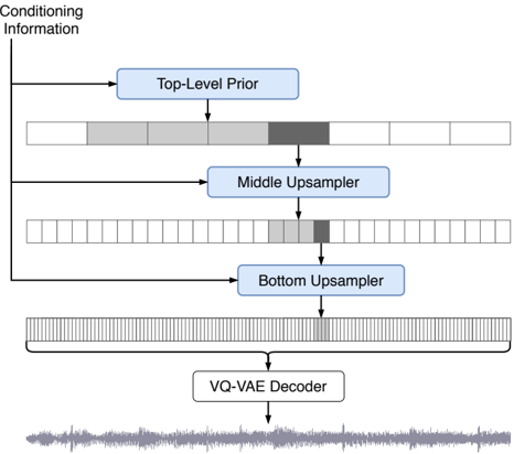Music Priors and Upsamplers After training the VQ-VAE, we need to learn a prior p ( z ) over the compressed space to generate samples. We break up the prior model as $$\frac { 1 } { p ( z ) } = p ( z ^ { top } , z ^ { middle } , z ^ { bottom } )$$ $$= p ( z ^ { top } ) p ( z _ { middle } | z ^ { top } ) p$$ and train separate models for the top-level prior p ( z top ) , and upsamplers p ( z middle | z top ) and p ( z bottom | z middle , z top ) . Each of these is an autoregressive modeling problem in the discrete token space produced by the VQ-VAE. We use Transformers with sparse attention (Vaswani et al., 2017; Child et al., 2019) as they are currently the SOTA in autoregressive modeling. We propose a simplified version which we call the Scalable Transformer, that is easier to implement and scale (see Appendix A for details). For the upsamplers, we need to provide the autoregressive Transformers with conditioning information from the codes of the upper levels. To do so, we use a deep residual WaveNet (Xie et al., 2017) followed by an upsampling strided convolution and a layer norm (Ba et al., 2016), and add the output as extra positional information to the embeddings of the current level. We condition the lower levels only on the chunk of upper level codes that correspond to the same segment of raw audio. At each level, we use Transformers over the same context length of discrete codes, which correspond to increasing the raw audio length with larger hop lengths, and modeling longer temporal dependencies at the higher levels while keeping the same computational footprint for training each level. As our VQ-VAE is convolutional, we can use the same VQ-VAE to produce codes for arbitrary lengths of audio. ## 4.1. Artist, Genre, and Timing Conditioning Our generative model can be made more controllable by providing additional conditioning signals while training. For our first models, we provide artist and genre labels for the songs. This has two advantages: first, it reduces the entropy of the audio prediction, so the model is able to achieve better quality in any particular style. Second, at generation time, we are able to steer the model to generate in a style of our choosing. Additionally, we attach a timing signal for each segment at training time. This signal includes the total duration of the piece, the start time of that particular sample and how much fraction of the song that has elapsed. This allows the model to learn audio patterns that depend on the overall structure, such as spoken or instrumental introductions and applause at the end of a piece. ## 4.2. Lyrics Conditioning While the conditioned models above are able to generate songs of diverse genres and artistic styles, singing voices generated by those models, while often sung in a compelling melody, are mostly composed of babbling, rarely producing recognizable English words. In order to be able to control the generative model with lyrics, we provide more context at training time by conditioning the model on the lyrics corresponding to each audio segment, allowing the model to produce singing simultaneosly with the music. Lyrics-to-singing (LTS) task : The conditioning signal only includes the text of the lyrics, without timing or vocalisation information. We thus have to model the temporal alignment of lyrics and singing, the artists voice and also the diversity of ways one can sing a phrase depending on the pitch, melody, rhythm and even genre of the song. The conditioning data isn't precise as the lyrics data often contains textual references to repeated sections like 'chorus' or mismatching portions of lyrics with the corresponding music. There is also no separation between lead vocals, accompanying vocals and the background music in target audio. This makes the Lyrics-to-singing (LTS) task significantly more challenging than the corresponding Text-to-speech (TTS) task. Providing lyrics for chunks of audio : Our dataset includes song-level lyrics, but to make the task easier we train on shorter (24 sec) chunks of audio. To provide the lyrics cor- <details> <summary>Image 2 Details</summary>  ### Visual Description ## Diagram: Hierarchical Generative Model Architecture ### Overview The image illustrates a hierarchical generative model architecture, likely designed for audio synthesis. The diagram depicts a flow where "Conditioning Information" is injected into three sequential processing stages (Top-Level Prior, Middle Upsampler, and Bottom Upsampler). These stages progressively increase the resolution of latent representations, which are then processed by a VQ-VAE (Vector Quantized Variational Autoencoder) Decoder to produce a final audio waveform. ### Components/Axes * **Input Source:** "Conditioning Information" (represented by a vertical line on the far left). * **Processing Blocks (Blue Rectangles):** * **Top-Level Prior:** Located at the top. * **Middle Upsampler:** Located in the center. * **Bottom Upsampler:** Located below the middle section. * **Latent Representation Bars (Horizontal):** * **Top Bar:** Low resolution (8 segments). * **Middle Bar:** Medium resolution (24 segments). * **Bottom Bar:** High resolution (dense grid, approximately 64+ segments). * **Output Block (White Rectangle):** "VQ-VAE Decoder" (bottom center). * **Final Output:** Audio waveform (bottom). ### Detailed Analysis The diagram follows a top-down flow, with specific interactions between the components: 1. **Conditioning Information:** This input is distributed horizontally to all three processing blocks (Top-Level Prior, Middle Upsampler, and Bottom Upsampler). 2. **Top-Level Prior:** * Receives "Conditioning Information." * Outputs to the first horizontal bar (8 segments). * The bar contains a highlighted region (one dark grey segment followed by three light grey segments). 3. **Middle Upsampler:** * Receives input from the "Top-Level Prior" (via the first bar) and "Conditioning Information." * Outputs to the second horizontal bar (24 segments). * The highlighted region from the top bar is propagated and expanded here (one dark grey segment followed by three light grey segments). 4. **Bottom Upsampler:** * Receives input from the "Middle Upsampler" (via the second bar) and "Conditioning Information." * Outputs to the third horizontal bar (dense grid). * The highlighted region is further propagated and expanded here. 5. **VQ-VAE Decoder:** * Takes the final, high-resolution latent representation from the third bar. * Produces the final audio waveform shown at the very bottom. ### Key Observations * **Resolution Scaling:** There is a clear hierarchical increase in resolution. The top bar has 8 segments, the middle has 24 (3x increase), and the bottom has a significantly higher density, suggesting a factor-of-3 or factor-of-4 upsampling at each stage. * **Information Propagation:** The specific pattern of shading (one dark grey cell followed by three light grey cells) acts as a visual marker for a specific latent feature or "token" being tracked and refined through the hierarchy. * **Global Conditioning:** The "Conditioning Information" is applied globally, meaning the model uses the same external context (e.g., text, class labels, or style) to guide the generation at every level of the hierarchy. ### Interpretation This diagram represents a **Hierarchical VQ-VAE** or a similar autoregressive audio generation model (such as Jukebox). * **The Logic:** The model separates the generation task into different temporal scales. The "Top-Level Prior" models the coarse, long-term structure of the audio (low resolution). The "Upsamplers" then fill in the details (medium and high resolution) based on the coarse structure and the conditioning information. * **Why it matters:** This architecture is necessary because generating raw audio (which has a very high sample rate, e.g., 44.1kHz) directly is computationally prohibitive. By compressing the audio into discrete latent codes (the bars) and generating them hierarchically, the model can maintain long-term coherence while efficiently generating high-fidelity audio. * **The "Reading Between the Lines":** The highlighted grey segments suggest that the model is not generating the entire sequence at once, but rather refining a specific "window" or "token" of information as it moves down the hierarchy, ensuring that the high-resolution output remains consistent with the low-resolution "plan" established by the Top-Level Prior. </details> - (a) Ancestral sampling : Priors for the VQ-VAE codes are trained using a cascade of Transformer models, shown in blue. Each model takes conditioning information such as genre, artist, timing, and lyrics, and the upsampler models are also conditioned on the codes from the upper levels. To generate music, the VQ-VAE codes are sampled from top to bottom using the conditioning information for control, after which the VQ-VAE decoder can convert the bottom-level codes to audio. 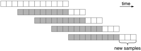- (b) Windowed sampling : To generate music longer than the model's context length (12 in this figure), we repeatedly sample continuations at each level, using overlapping windows of previous codes as the context. The overlap amount is a hyperparameter, and the figure shows an example of 75% overlap with hop length 3. 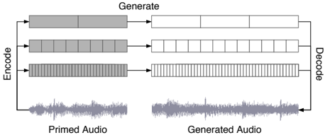- (c) Primed sampling : The model can generate continuations of an existing audio signal by converting it into the VQ-V AE codes and sampling the subsequent codes in each level. <details> <summary>Image 3 Details</summary>  ### Visual Description ## Diagram: Sliding Window Buffer Update ### Overview The image is a schematic diagram illustrating a temporal data processing mechanism, specifically a "sliding window" or buffer update process. It visualizes how a fixed-size data buffer is updated over five discrete time steps, where new data is shifted into the buffer while old data is discarded. ### Components/Axes * **Data Rows:** There are five horizontal rows, each containing 12 rectangular boxes. * **Shading:** * **White Boxes:** Represent new or unpopulated data slots. * **Grey Boxes:** Represent existing, processed, or populated data. * **Labels:** * **"time"**: Located at the top right, accompanied by an arrow pointing to the right, indicating the direction of temporal progression. * **"new samples"**: Located at the bottom right, with a bracket spanning the final four boxes of the bottom-most row. ### Detailed Analysis The diagram displays a consistent, staggered progression from top to bottom. Each row represents a subsequent time step. * **Row 1 (Top):** Contains 12 white boxes. This represents the initial state or an empty buffer. * **Row 2:** Contains 8 grey boxes followed by 4 white boxes. The row is shifted to the right by 3 units relative to Row 1. * **Row 3:** Contains 8 grey boxes followed by 4 white boxes. The row is shifted to the right by 3 units relative to Row 2 (or 6 units relative to Row 1). * **Row 4:** Contains 8 grey boxes followed by 4 white boxes. The row is shifted to the right by 3 units relative to Row 3 (or 9 units relative to Row 1). * **Row 5 (Bottom):** Contains 8 grey boxes followed by 4 white boxes. The row is shifted to the right by 3 units relative to Row 4 (or 12 units relative to Row 1). * **"New Samples" Bracket:** This bracket is positioned under the final 4 white boxes of the bottom row, explicitly identifying these as the incoming data points for that time step. ### Key Observations * **Consistent Window Size:** The total number of boxes in each row remains constant at 12. * **Fixed Update Rate:** The buffer shifts by exactly 3 units (or 25% of the total buffer size) at each time step. * **Overlap:** The grey (processed) data persists across rows, shifting position, which is characteristic of overlapping window processing (e.g., in Short-Time Fourier Transforms or audio signal processing). ### Interpretation This diagram demonstrates a **sliding window buffer update mechanism**. In technical contexts, this is used to process continuous data streams in chunks. The "grey" area represents the data currently held in memory or the processing window. As time progresses (moving down the rows), the oldest data is dropped from the left, and new data (the "new samples") is shifted in from the right. The specific overlap (3 units of shift for a 12-unit window) suggests a 75% overlap between consecutive processing windows. This technique is commonly employed in digital signal processing (DSP) to ensure continuity in data analysis, preventing edge artifacts or data loss that might occur if windows were processed without overlap. </details> <details> <summary>Image 4 Details</summary>  ### Visual Description ## Diagram: Hierarchical Audio Generation Process ### Overview This diagram illustrates a multi-scale, hierarchical audio generation process. It depicts how input audio ("Primed Audio") is encoded into discrete representations at varying levels of granularity, transformed through a generation process, and subsequently decoded back into an audio waveform ("Generated Audio"). The diagram highlights a feedback loop, suggesting an autoregressive or iterative generation mechanism. ### Components/Axes * **Top Center:** "Generate" (Label indicating the transformation process from grey to white blocks). * **Left Side:** "Encode" (Vertical label with a bracket encompassing the three rows of grey blocks). * **Right Side:** "Decode" (Vertical label with a bracket encompassing the three rows of white blocks). * **Bottom Left:** "Primed Audio" (Label for the input waveform). * **Bottom Right:** "Generated Audio" (Label for the output waveform). * **Visual Elements:** * **Grey Blocks (Left):** Represent the encoded state of the primed audio. * **White Blocks (Right):** Represent the generated state of the audio. * **Waveforms:** Visual representations of audio signals at the bottom. * **Arrows:** Indicate the flow of data from input to output, and a feedback loop from output back to input. ### Detailed Analysis The diagram is structured into three distinct horizontal rows, representing different levels of temporal resolution or semantic hierarchy: * **Row 1 (Top):** * **Input (Grey):** 2 blocks. * **Output (White):** 3 blocks. * **Trend:** Represents the coarsest level of representation. * **Row 2 (Middle):** * **Input (Grey):** 8 blocks. * **Output (White):** 9 blocks. * **Trend:** Represents an intermediate level of detail. * **Row 3 (Bottom):** * **Input (Grey):** High density (approx. 30+ blocks). * **Output (White):** High density (approx. 30+ blocks). * **Trend:** Represents the finest level of detail (likely sample-level or high-resolution acoustic features). **Flow and Connectivity:** 1. **Input:** The "Primed Audio" waveform is processed by the "Encode" stage, resulting in the three rows of grey blocks. 2. **Transformation:** The "Generate" process maps the grey blocks to the white blocks across all three hierarchical levels. 3. **Output:** The "Decode" stage converts the white blocks into the "Generated Audio" waveform. 4. **Feedback Loop:** A line connects the "Generated Audio" back to the input of the "Encode" stage, indicating that the output is fed back into the system, likely to continue the generation process (autoregression). ### Key Observations * **Hierarchical Granularity:** The diagram explicitly demonstrates a "coarse-to-fine" or "multi-scale" approach. The top row has the fewest blocks, while the bottom row has the most, suggesting the model processes audio at different temporal resolutions simultaneously. * **Feedback Mechanism:** The loop-back arrow is critical; it implies that the generation is not a single-pass operation but an iterative one where the model conditions its next step on its previous output. * **Symmetry:** The "Encode" and "Decode" processes are visually symmetrical, suggesting a standard encoder-decoder architecture (such as a VQ-VAE or similar neural audio codec). ### Interpretation This diagram represents the architecture of a **hierarchical neural audio generation model** (similar to AudioLM or SoundStream). * **Why it matters:** By breaking audio into hierarchical levels (coarse to fine), the model can capture long-term structure (the top rows) and fine-grained acoustic detail (the bottom row) more efficiently than processing raw audio samples directly. * **Reading between the lines:** The feedback loop indicates this is an **autoregressive model**. The system generates a small chunk of audio, appends it to the "Primed Audio," and feeds it back into the encoder to generate the next chunk. This is the standard mechanism for generating long-form, coherent audio (like speech or music) where the model must "remember" what it just generated to maintain consistency. The discrepancy in block counts between the grey and white rows (e.g., 2 vs 3) suggests the model may be performing upsampling or temporal expansion during the generation phase. </details> Figure 2. Sampling methods for generating music responding to the audio during training, we began with a simple heuristics of aligning the characters of the lyrics to linearly span the duration of each song, and pass a fixed-side window of characters centered around the current segment during training. While this simple strategy of linear alignment worked surprisingly well, we found that it fails for certain genres such as hip-hop with fast lyrics. To address this, we use Spleeter (Hennequin et al., 2019) to extract vocals from each song and run NUS AutoLyricsAlign (Gupta et al., 2020) on the extracted vocals to obtain a word-level alignments of the lyrics, allowing us to more accurately provide the lyrics for a given chunk of audio. We choose a large enough window so that the actual lyrics have a high probability of being inside the window. 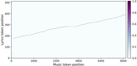Encoder-decoder model : We use an encoder-decoder style model to condition on the characters of the lyrics, with the encoder producing features from the lyrics which are attended to by the decoder which produces the top level music tokens. The lyrics encoder is a Transformer with an autoregressive modeling loss for lyrics, and its last level is used as features of the lyrics. In the music decoder, we interleave a few additional layers with encoder-decoder attention where the queries from the music tokens are only allowed to attend to keys and values from the lyrics tokens. These layers attend on the activation from the last layer of the lyrics encoder (see Figure 8c). In Figure 3, we see that the attention pattern learned by one of these layers corresponds to the alignment between the lyrics and the singing. ## 4.3. Decoder Pretraining To reduce computation required to train the lyrics conditional model, we use a pretrained unconditional top-level prior as our decoder and introduce the lyrics encoder using model surgery (Berner et al., 2019). We initialize the output projection weights in the MLP and the attention layers of these residual blocks to zeros (Zhang et al., 2019a), so that the added layers perform the identity function at initialization. Thus, at initialization the model behaves identically as the pretrained decoder, but there is still a gradient with respect to the encoder state and parameters 2 , allowing the model to learn to use the encoder. ## 4.4. Sampling After we have trained our VQ-VAE, upsamplers, and top level priors, we can then use them to sample novel songs. Ancestral sampling : We first generate the top level codes one token at a time by the usual ancestral sampling process (see Figure 2a): generating the first token, then passing all 2 The gradient also needs to break symmetry with the encoder output features, which is the case here since the weights of the input projections in the attention are not zero. Figure 3. Lyrics-singing alignment learned by one of the encoderdecoder attention layers. The x -axis is the position of music queries, and the y -axis is the position of lyric keys. The positions attended to by the decoder correspond to the characters being sung. <details> <summary>Image 5 Details</summary>  ### Visual Description ## Heatmap: Music Token Position vs. Lyrics Token Position Alignment ### Overview This image is a 2D heatmap visualization, likely representing an attention map or alignment matrix from a machine learning model (such as a Transformer-based architecture). It plots the relationship between "Music token position" (x-axis) and "Lyrics token position" (y-axis). The visualization demonstrates how the model aligns specific segments of music with corresponding lyrical content over time. ### Components/Axes * **X-Axis (Horizontal):** Labeled "Music token position". The scale ranges from 0 to 8000, with major tick marks at 0, 1600, 3200, 4800, 6400, and 8000. * **Y-Axis (Vertical):** Labeled "Lyrics token position". The scale ranges from 0 to 500, with major tick marks at 0, 100, 200, 300, 400, and 500. * **Legend (Right side):** A vertical color bar representing the intensity of the alignment/attention score. * **0.0 (White):** Indicates no or minimal alignment/attention. * **1.0 (Dark Purple):** Indicates high alignment/attention. * **Main Plot Area:** A central region displaying a diagonal line of varying intensity (light blue to dark purple) against a near-white background. ### Detailed Analysis * **Trend Verification:** The primary data series is a continuous, slightly jagged diagonal line that slopes upward from the bottom-left quadrant toward the top-right quadrant. This indicates a monotonic, positive correlation: as the music token position increases, the lyrics token position also increases. * **Data Points (Approximate):** * **Start Point:** The alignment begins at approximately (x=200, y=180). * **End Point:** The alignment terminates at approximately (x=8200, y=400). * **Slope:** The line covers a range of ~8000 music tokens for ~220 lyrics tokens (400 - 180). This indicates a significantly higher density of music tokens compared to lyrics tokens. * **Visual Characteristics:** * The line is not perfectly smooth; it exhibits small, step-like discontinuities. * There are faint, scattered artifacts (low-intensity noise) visible off the main diagonal, particularly in the lower-left and mid-right regions, suggesting minor, non-primary attention weights. ### Key Observations * **Asymmetry:** The x-axis (8000) is significantly longer than the y-axis (500), indicating that the music sequence is roughly 16 times longer in terms of token count than the lyrics sequence. * **Discontinuities:** The "steps" in the diagonal line suggest that the alignment is not strictly linear. These breaks likely correspond to structural changes in the audio (e.g., instrumental breaks, chorus/verse transitions, or pauses) where the lyrics do not progress at a constant rate relative to the music. * **Intensity:** The line is generally light-to-medium purple, suggesting that while there is a clear alignment, the attention is distributed rather than highly concentrated on single points. ### Interpretation This visualization demonstrates the temporal alignment between a music sequence and its corresponding lyrics. * **Model Behavior:** The diagonal structure confirms that the model has successfully learned the temporal progression of the song. It understands that later music tokens correspond to later lyrics tokens. * **Structural Insights:** The discontinuities in the diagonal are the most significant feature. In a musical context, these likely represent sections where the lyrics are sparse or absent (instrumental sections), causing the "Lyrics token position" to plateau while the "Music token position" continues to advance. * **Peircean Investigative Note:** The presence of faint, off-diagonal noise suggests that the model is not perfectly confident in its alignment at all times, or that there is a degree of "soft attention" where the model considers multiple potential alignments simultaneously. The overall trend is highly robust, indicating a successful training outcome for sequence alignment. </details> previously generated tokens into the model as inputs and outputting the next token conditioned on all previous tokens. We then run our conditioning wavenet on the top level codes to produce the conditioning information for the middle level and sample ancestrally from it too, and do the same for the bottom level. Windowed sampling : To sample segments longer than the context length, we use windowed sampling, where we move ahead our sampling window by half our context and continue sampling conditioned on this half context (See Figure 2b). We can trade off speed for quality by using a smaller hop length here. Primed sampling : Instead of sampling the entire token sequence from the model, we can also run a forward pass of the VQ-VAE to obtain the top, middle, and bottom level codes corresponding to a segment from an actual song, as shown in Figure 2c. We can use these as the initial tokens in our ancestral sampling process and continue sampling from these to produce novel completions of the song. ## 5. Experiments ## 5.1. Dataset We scraped a new dataset of 1.2 million songs (600k of which in English), paired with the lyrics and metadata from LyricWiki (LyricWiki). The metadata includes artist, album, genre, and year of the release, along with common moods or playlist keywords associated with each song. We train on 32 bit, 44.1 kHz raw audio and perform data augmentation by randomly downmixing the right and left channels to produce mono channel audio. ## 5.2. Training Details For the music VQ-VAE, we use 3 levels of bottlenecks compressing 44 kHz audio in dimensionality by 8x, 32x, and 128x respectively, with a codebook size of 2048 for each level. The VQ-VAE has 2 million parameters and is trained on 9-second audio clips on 256 V100 for 3 days. We used exponential moving average to update the codebook following Razavi et al. (2019). For our prior and upsampler models, we use a context of 8192 tokens of VQ-VAE codes, which corresponds to approximately 24, 6, and 1.5 seconds of raw audio at the top, middle, and bottom level, respectively. The upsamplers have one billion parameters and are trained on 128 V100s for 2 weeks, and the top-level prior has 5 billion parameters and is trained on 512 V100s for 4 weeks. We use Adam with learning rate 0 . 00015 and weight decay of 0 . 002 . For lyrics conditioning, we reuse the prior and add a small encoder, after which we train the model on 512 V100s for 2 weeks. The detailed hyperparameters for our models and training are provided in Appendix B.3. ## 5.3. Samples We trained a sequence of models with increasing sample quality. Our first model was trained on the MAESTRO dataset using 22 kHz VQ-VAE codes and relatively small prior models. We observed that this could generate high fidelity classical music samples with piano and occasional violin. We then collected a larger and more diverse dataset of songs with genre and artist labels. The same model when trained on this new dataset was able to produce diverse samples other than classical music, and demonstrated musicality and coherence over more than a minute. Despite the novelty of being able to generate generally high fidelity and coherent songs, sample quality was still limited by a number of factors. First, the use of 22 kHz sampling rate along with small upsamplers introduced noise both in the upsampling and decoding steps, which we hear as grainy texture. We improved fidelity by using 44 kHz VQ-VAE and 1B parameter upsamplers in all subsequent experiments at the expense of longer rendering time. Second, the 1B top-level prior was not big enough to produce singing and diverse musical timbres. We first explored increasing the model size to 5 billion parameters. Larger capacity allowed better modeling of the broader distribution of songs, resulting in samples with better musicality, longer coherence and initial singing. While there is an overall qualitative improvement, the unconditional model still struggled to sing recognizable words. Training a seq2seq model with lyric conditioning and limiting the dataset only to songs primarily in English made singing both intelligible and controllable. The final model, which we call Jukebox, uses all these improvements. Because everyone experiences music differently, it is generally tricky and not very meaningful to evaluate samples by the mean opinion score or FID-like metrics. We manually evaluate coherence, musicality, diver- sity, and novelty of generated samples. The links to curated examples are embedded in text. Coherence: We find the samples stay very coherent musically through the context length of the top-level prior (approximately 24 seconds), and they maintain similar harmonies and textures as we slide the window to generate longer samples. However, because the top-level does not have the context of the entire song, we do not hear long term musical patterns, and we would never hear choruses or melodies that repeat. The generations progress through beginnings of songs (for example applause or slow instrumental warm-ups), through sections that sound chorus-like, through instrumental interludes, and then fading or otherwise wrapping up at the end. The top-level prior always knows what fraction of the song is complete time-wise, so it is able to imitate appropriate beginnings, middles and ends. Musicality: The samples frequently imitate familiar musical harmonies and the lyrics are usually set in ways that are very natural. Frequently the highest or longest notes of the melody match words that a human singer would choose to emphasize, and the lyrics are almost always rendered in ways that capture the prosody of the phrases. This is noticeable in hip hop generations, where the model reliably captures the rhythm of spoken text. We do find that the generated melodies are usually less interesting than human composed melodies. In particular, we do not hear the antecedent and consequent pattern familiar to many human melodies, and we rarely hear choruses that are melodically memorable. Diversity: Likelihood training encourages covering of all modes, so we expect the model to produce diverse samples. - Re-renditions: Wegenerate multiple samples conditioned on artist and lyrics combinations that exist in our training data. While occasionally drum and bass lines or melodic intervals echo the original versions, we find that none of the generated samples is noticeably similar to the original songs. We also generate multiple songs conditioned on the same artist and lyrics as Sample 1 to obtain Samples 9-12. All five sound interesting in their own ways with different moods and melodies with Sample 10 playing a harmonic at 00:14 as part of a blues riff, showing that the model has learned a wide range of singing and playing styles. - Completions: We prime the model with 12 seconds of existing songs and ask it to complete them in the same styles. When the priming samples include singing, the continuations are more likely to imitate the original tunes and rhythms. Songs primed with more generic or common intros tend to be more diverse. Even generated samples that are close to the originals early on deviate completely into new musical material after about 30 seconds. Re-renditions and completions are interesting and diverse, but overall, there is still room for improvement in music quality compared to the original songs. - Full tree: To understand diversity in a more systematic way, we generate multiple continuations from the same segment. We start with a one-minute sample and independently sample four times per one-minute extension. By the three minute mark, there are 16 completions. We can think of this branching tree as exploring different possibilities obtained by ancestral sampling. In the generated songs in the link, we hear diversity in singing and development even when the same initial segment is used. We note that this particular sample follows the lyrics more successfully than many. For certain genres like hip hop and rap, where linearly moving the window does not yield good lyrics alignment, the chance of obtaining plausible singing is lower. Novelty: With the ability to condition on various styles, lyrics, and raw audio, we would like Jukebox to be a useful tool for both professional musicians and music enthusiasts alike. In this section, we are interested in exploring capabilities and applications of Jukebox. - Novel styles: We generate songs in an unusual genre typically not associated with an artist. In general, we find that it is fairly difficult to generalize to a novel style of singing while using the same voice as the artist embedding overpowers other information. In Joe Bonamassa and Frank Sinatra samples, we hear a modest variation in instrumentation, energy, and ambience depending on the genre embedding. However, our attempts to mix country singer Alan Jackson with unusual genres like hip hop and punk did not seem to move the samples away from a country style in meaningful ways. - Novel voices: Wepick artists whose voices are reproduced reasonably well by the model, and interpolate their style embeddings to synthesize new voices. Some blending, for instance, between Frank Sinatra and Alan Jackson in Sample 4, still sounds similar to Frank Sinatra. In most cases, the model renders in a vaguely recognizable but distinct voice that preserves different vocal attributes. Samples 1 and 2 conditioned on the Céline Dion embeddings divided by two have slightly different timbre and tone but capture her unique vibrato. We also experiment with changing the style embedding in the middle of a song to create a duet (Sample 7). This is another way of guiding generation during sampling. Continuing in another voice works best when the segment ends in an interlude; otherwise, the model blends voices in the middle of a word or a sentence. - Novel lyrics: We ask Jukebox to sing poems and novel verses generated by GPT-2 (Radford et al.) to demonstrate that it can indeed sing new lyrics. While the training data consists of song lyrics with limited vocabulary and constrained structure, the model has learned to follow along most prompts and sing even new words that are reasonably pronounceable (including technical terms from the deep learning literature). To get the best results, however, we find that it is useful to spell out difficult words or acronyms as they are spoken. The generations are noticeably higher quality if the text matches the distribution of lyrics for the given artist, both in terms of length, and of rhyming or rhythmic qualities. For example, hip hop lyrics tend to be longer than most other genres, and the commonly emphasized syllables easily form clear rhythms. - Novel riffs: Another useful application of Jukebox is the ability to record an incomplete idea and explore various continuations without ever needing to tabulate in symbolic representations, which would lose details of timbre and mood. We curate recordings of novel riffs by our in-house musicians and prime the model during sampling. Sample 6 starts with a musical style not widely used in Elton John's songs. The model still carries out the tune and develops it further. Similarly, the beginning of Sample 1 is a progressive jazz piece with a 5/4 polymeter, which has never been used in hip hop. Despite this novelty, the rhythm persists throughout the song and is incorporated naturally with rapping. ## 5.4. VQ-VAE Ablations Table 1. Reconstruction fidelity degrades with higher compression. Restarting dead codes near random encoder outputs mitigates learning suboptimal codes. | | | Spectral convergence (dB) | Spectral convergence (dB) | |------------|------------|-----------------------------|-----------------------------| | Level | Hop length | Without restart | With restart | | Bottom | 8 | - 21 . 1 | - 23 . 0 | | Middle Top | 32 | - 12 . 4 | - 12 . 4 | | | 128 | - 8 . 3 | - 8 . 3 | Table 2. Bottom-level VQ-VAE reconstruction results with different codebook sizes. Using larger codebooks helps reconstruction because it allows more information to be encoded at the bottleneck layers. Removing the bottleneck entirely yields almost perfect reconstruction. | Codebook size | Spectral convergence (dB) | |-----------------|-----------------------------| | 256 | - 15 . 9 | | 2048 | - 23 . 0 | | No quantization | - 40 . 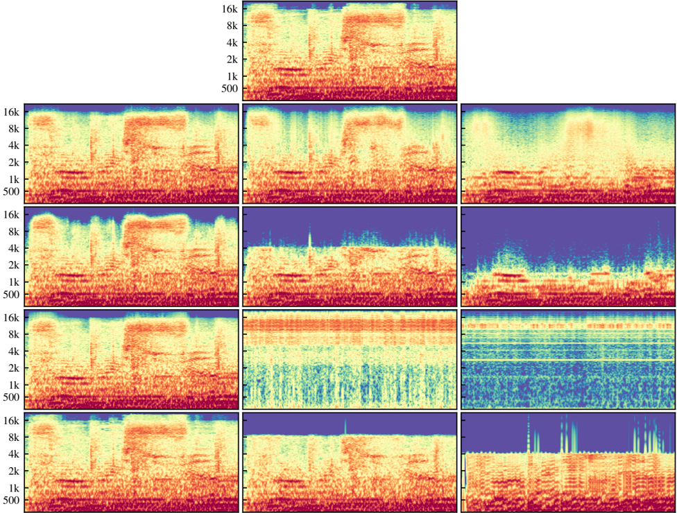5 | Figure 4. Comparison of reconstructions from different VQ-VAEs, x-axis is time and y-axis is frequency. The columns from left to right are bottom-, middle-, and top-level reconstructions at hop lengths 8, 32, and 128 respectively, visualized as Mel spectrograms. The first row is the ground-truth, and the second row shows the spectrograms of audio outputs from our VQ-VAE. In the third row, we remove the spectral loss, and see that the middle and top level lose high-frequency information. In the fourth row, we use a hierarchical VQ-VAE (Razavi et al., 2019) instead of separate auto-encoders (Figure 1), and we see the middle and top levels are not used for encoding pertinent information. Finally, the fifth row shows a baseline with the Opus codec that encodes audio at constant bitrates comparable to our VQ-VAE. It also fails to capture higher frequencies and adds noticeable artifacts at the highest level of compression. <details> <summary>Image 6 Details</summary>  ### Visual Description ## Spectrogram Grid: Audio Signal Processing Comparison ### Overview This image displays a grid of 13 spectrograms, likely representing a comparison of audio signal processing techniques, generative model outputs, or noise reduction algorithms. The top row contains a single spectrogram, while the subsequent four rows each contain three spectrograms. The leftmost column (Rows 2–5) appears to be a consistent reference signal (Ground Truth), while the middle and right columns display various processed versions of that signal, exhibiting different spectral characteristics, filtering effects, and artifacts. ### Components/Axes * **Y-Axis (Frequency):** Logarithmic scale, labeled with the following markers (from bottom to top): 500, 1k, 2k, 4k, 8k, 16k. * **X-Axis (Time):** Unlabeled, representing the temporal progression of the audio signal. * **Color Mapping:** The heat map uses a standard spectrogram color scale: * **Dark Blue/Purple:** Low energy/silence. * **Red/Orange:** Moderate energy. * **Yellow/White:** High energy/peaks. ### Detailed Analysis The grid is organized into a 5-row structure. We will define the positions as (Row, Column). **Row 1:** * **(1, 1):** The reference spectrogram. It shows a full-spectrum signal with significant energy across the 500Hz to 16kHz range. **Row 2:** * **(2, 1):** Matches the reference signal in (1, 1). * **(2, 2):** Similar to the reference, but with slightly reduced high-frequency energy above 12kHz. * **(2, 3):** Exhibits a clear low-pass filter effect; energy is significantly attenuated above 8kHz. **Row 3:** * **(3, 1):** Matches the reference signal. * **(3, 2):** Shows a sharp spectral cutoff at approximately 4kHz. * **(3, 3):** Significant signal degradation. The signal is mostly confined below 2kHz, with high-frequency noise or "hiss" artifacts visible above 2kHz. **Row 4:** * **(4, 1):** Matches the reference signal. * **(4, 2):** Displays distinct horizontal spectral lines (harmonic artifacts) across the entire frequency range, suggesting a reconstruction or quantization error. * **(4, 3):** Very sparse spectral content. It shows horizontal lines (tones) and a lack of the complex, broadband structure seen in the reference. **Row 5:** * **(5, 1):** Matches the reference signal. * **(5, 2):** Shows a sharp cutoff at approximately 8kHz, with some vertical transient artifacts. * **(5, 3):** Shows a sharp cutoff at approximately 4kHz, with distinct vertical "chirp" or transient artifacts extending into the higher frequencies. ### Key Observations * **Reference Consistency:** The leftmost column (Rows 2–5) is identical to the top row, serving as the control or "Ground Truth" signal. * **Spectral Filtering:** Several plots (e.g., 3,2; 5,3) demonstrate aggressive low-pass filtering, effectively removing information above 4kHz. * **Artifact Generation:** Plots (4,2) and (4,3) show evidence of harmonic distortion or "spectral lines," which are common artifacts in lossy compression or generative audio models. * **Energy Distribution:** The reference signal is broadband, whereas the processed signals show varying degrees of "spectral holes" (missing frequency bands) and noise floor elevation. ### Interpretation This image is characteristic of a figure from a technical paper evaluating audio synthesis or enhancement models (e.g., GANs, Diffusion models, or Vocoders). * **What the data demonstrates:** The grid illustrates how different models or processing parameters affect the frequency content of an audio signal. The leftmost column provides the target, while the other columns show the "reconstruction" quality of various methods. * **Why it matters:** In audio engineering and machine learning, preserving the full frequency spectrum (up to 16kHz+) is critical for high-fidelity audio. The variations in the middle and right columns highlight specific failure modes: * **Low-pass filtering:** Loss of "air" or high-frequency detail. * **Spectral lines:** Audible metallic or robotic artifacts. * **Noise floor elevation:** Audible hiss or background interference. * **Peircean Investigative Note:** The progression from the top-left reference to the increasingly degraded signals in the bottom-right suggests a comparative study where the models are ranked or categorized by their ability to reconstruct the original signal without introducing the artifacts observed in the rightmost column. </details> Table 3. Top-level codes are generally difficult to train well without spectral loss or with a single hierarchical autoencoder. Resulting reconstructions may lose some to most of information. | Ablation | Spectral convergence (dB) | |-------------------------|-----------------------------| | None | - 8 . 3 | | Without spectral loss | - 6 . 3 | | With single autoencoder | 2 . 9 | We compare raw audio VQ-VAEs when trained with varying compression ratios, objectives, and architectures. As we use nonautoregressive decoders with continuous representation for output, we report spectral convergence (Sturmel & Daudet, 2011), which measures the amount of spectral error relative to signal, as test error and proxy for reconstruction fidelity. We evaluate on 5000 held-out 3-second audio segments and report the average in decibels. All models in this section are trained with a batch size of 32, 3-second audio clips sampled at 44 kHz. As before, we use hop lengths of 8, 32, and 128 for the bottom, middle and top level respectively. In Table 1, we see that increasing the hop size results in higher reconstruction error. Figure 4 indeed shows that a significant amount of information, especially higher frequencies, is missing at middle and top levels across all ablations we ran. 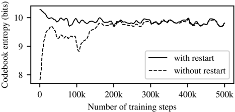This is expected as audio is compressed more with Figure 5. Entropy of codebook with 2048 codes, i.e 11 bits, over training. Reviving dead codes near random encoder outputs ensures good codebook utilization from the start of training. <details> <summary>Image 7 Details</summary>  ### Visual Description ## Line Chart: Codebook Entropy vs. Training Steps ### Overview This image displays a line chart comparing the "Codebook entropy (bits)" over the course of 500,000 training steps for two distinct experimental conditions: "with restart" and "without restart." The chart illustrates how the entropy of the codebook evolves during the training process, highlighting a significant divergence in early training stages followed by convergence. ### Components/Axes * **Y-Axis:** Labeled "Codebook entropy (bits)". The scale ranges from 8 to 10, with tick marks at 8, 9, and 10. * **X-Axis:** Labeled "Number of training steps". The scale ranges from 0 to 500k, with major tick marks at 0, 100k, 200k, 300k, 400k, and 500k. * **Legend:** Positioned in the middle-right area of the chart. * **Solid line:** Represents "with restart". * **Dashed line:** Represents "without restart". ### Detailed Analysis The chart tracks two data series across 500,000 steps: **1. Solid Line ("with restart")** * **Trend:** The line begins at a high entropy value of approximately 10.3 at step 0. It exhibits a rapid downward trend until approximately 50k steps, where it reaches a value of roughly 9.9. From 50k steps through 500k steps, the line remains relatively stable, oscillating within a narrow band between 9.7 and 9.9. **2. Dashed Line ("without restart")** * **Trend:** The line begins at a very low entropy value of approximately 7.8 at step 0. It rises sharply between 0 and 40k steps, reaching a local peak of approximately 9.6. Following this, it experiences a period of instability: * It dips to approximately 9.3 around 60k steps. * It drops further to a local minimum of approximately 8.8 at 100k steps. * It then rises sharply between 100k and 150k steps, recovering to approximately 9.7. * From 200k steps to 500k steps, the dashed line tracks very closely with the solid line, oscillating in the same 9.7–9.9 range. ### Key Observations * **Early Divergence:** There is a stark difference in behavior between the two models before the 200k step mark. The "with restart" model maintains high entropy from the start, whereas the "without restart" model starts with low entropy and undergoes a significant "dip" (collapse) around 100k steps. * **Convergence:** By the 200k step mark, both models converge to a similar entropy level. * **Stability:** The "with restart" model demonstrates higher stability in the early phases of training compared to the "without restart" model. ### Interpretation This data is characteristic of training dynamics in vector quantization models (such as VQ-VAEs). * **Codebook Collapse:** The low entropy at the start of the "without restart" line (and the dip at 100k) suggests that the model is suffering from "codebook collapse," where only a small subset of the available codebook vectors are being utilized. * **The Role of "Restart":** The "with restart" mechanism appears to be a technique designed to prevent this collapse. By resetting the codebook or the model state, the system forces the model to utilize a wider variety of codes early on, maintaining higher entropy. * **Long-term Equivalence:** The fact that both lines converge after 200k steps suggests that while the "restart" mechanism is crucial for avoiding early-stage failure or poor initialization, it may not significantly alter the final capacity or entropy limit of the model once it has successfully stabilized. The "restart" is essentially a "safety net" for the initial training phase. </details> larger hop sizes. To mitigate codebook collapse, we restart dead codes near random encoder embeddings. In Figure 5, we see that this yields higher codebook usage even from early on in training. Models trained without random restarts can converge to the same test error and codebook usage but require more training steps. With poor initialization, these models sometimes end up with suboptimal codes hurting reconstruction fidelity. Codebook size also matters, as it sets a limit on channel capacity through the bottleneck layers. In Table 2, we find that reconstruction error increases considerably when the codebook size is reduced from 2048 to 256. We also compare with a model that uses continuous representations without vector quantization. We can think of this model as using a vastly large codebook with all encoder embeddings. This achieves almost perfect reconstruction with negligible spectral error. When the model is trained with L2 loss only, reconstructions tend to sound muddy from missing high frequencies, and this problem is exacerbated as hop size is increased. In Figure 4, we see that top-level codes trained without spectral loss do not capture much information beyond 2 kHz, and obtain worse reconstructions (Table 3). However, we observe that while spectral loss helps encode more information, it also adds distortion artifacts which we hear as scratchy noise. Lastly, we train a raw audio hierarchical VQ-VAE (Razavi et al., 2019) and find that it is generally difficult to push information to higher levels. This model is trained twice as long as the previous models, but middle and top-level reconstructions as shown in Figure 4 are not capturing much. It is possible that higher level codes may have collapsed before bottom level starts to reconstruct the audio well. Making the bottom layers explicitly model residuals pushed more information to the top. But, we found separate autoencoders to be cleaner and more effective. ## 6. Related Work Generative modeling in deep learning: Generative models aim to learn the distribution of data by either explicitly by modeling the distribution or implicitly by constructing means to sample from it (Goodfellow, 2016). Modeling the interdependency within high-dimensional data was traditionally considered extremely difficult, but starting with Deep Boltzmann Machines (Salakhutdinov & Hinton, 2009), various kinds of deep generative models have been introduced. Generative Adversarial Networks (GANs) (Goodfellow et al., 2014) use generator and discriminator networks that contest each other to make the generated samples as indistinguishable as possible from the data, and they are renowned for their ability to generate high-quality pictures (Zhang et al., 2019b; Brock et al., 2019). Autoregressive generative models such as NADE (Uria et al., 2016), PixelCNN (Van den Oord et al., 2016), and Transformers (Vaswani et al., 2017) use the chain rule of probability to factorize the joint distribution of data into a product of simpler distributions, and flow-based models (Dinh et al., 2015; 2017; Rezende & Mohamed, 2015; Kingma & Dhariwal, 2018) learn a series of invertible transformations that maps the data distribution with a simpler one such as a Gaussian distribution. Autoregressive flows (Papamakarios et al., 2017; Kingma et al., 2016) combine the two ideas to achieve faster density estimation or data generation. Variational autoencoders (VAEs) (Rezende et al., 2014; Kingma & Welling, 2014) impose a Gaussian prior on the latent code in an encoder-decoder setup from which data can be sampled. Generative models for music: Generative modeling of symbolic music dates back to more than half a century, when Hiller Jr & Isaacson (1957) introduced the first computergenerated music based on Markov chains. There exists a variety of earlier approaches using rule-based systems (Moorer, 1972), chaos and self-similarity (Pressing, 1988), cellular automata (Beyls, 1989), concatenative synthesis (Jehan, 2005), and constraint programming (Anders & Miranda, 2011). More recent data-driven approaches include DeepBach (Hadjeres et al., 2017) and Coconet (Huang et al., 2017) which use Gibbs sampling to produce notes in the style of Bach chorals, MidiNet (Yang et al., 2017) and MuseGAN (Dong et al., 2018) which use generative adversarial networks, MusicVAE (Roberts et al., 2018) and HRNN (Wu et al., 2019) which use hierarchical recurrent networks, and Music Transformer (Huang et al., 2019a) and MuseNet (Payne, 2019) which use Transformers to autoregressively predict MIDI note events. There also have been a number of approaches for synthesizing music conditioned on symbolic music information, such as NSynth (Engel et al., 2017) which uses WaveNet-style autoencoder, Mel2Mel (Kim et al., 2019) and Wave2Midi2Wave (Hawthorne et al., 2019) which synthesize music using WaveNet conditioned on a piano roll representation, and GanSynth (Engel et al., 2019) which uses generative adversarial networks to produce magnitude spectrograms together with instananeous frequencies for easier spectrogram inversion. Generative models for music can also be used for music style transfer, as seen in Midi-V AE (Brunner et al., 2018) which uses a variational autoencoder to transfer styles between classical and jazz music, LakhNES (Donahue et al., 2019) which uses a Transformer architecture to generate chiptune music, and Universal Music Translator Network (Mor et al., 2019) which uses a denoising autoencoder that can disentangle musical style and content. Sample-level generation of audio: In recent years, a variety of generative models for raw audio have been introduced. WaveNet (Oord et al., 2016) performs autoregressive sampleby-sample probabilistic modeling of raw waveform using a series of dilated convolutions to exponentially increase the context length. It can produce realistic audio either unconditionally or by conditioning on acoustic features or spectrograms. The autoregressive nature of WaveNet makes the sampling notoriously slow, and it uses a categorical distribution for audio samples which introduces quantization noise. Parallel WaveNet (Oord et al., 2018) improves upon this by instead using a mixture of logistics distribution, a continuous probability distribution, and performing probability density distillation which learns a parallel feed-forward network from a pre-trained autoregressive model, allowing faster sampling of high fidelity audio. ClariNet (Ping et al., 2019) achieves similar audio quality using a simple Gaussian distribution instead and thus having a closed-form loss function, eliminating the need for Monte-Carlo sampling. SampleRNN (Mehri et al., 2017) uses a multi-scale, hierarchical recurrent neural network with convolutional upsampling to model long-range complex structures. WaveRNN (Kalchbrenner et al., 2018) uses recurrent neural networks that operate separately on the most significant and the least significant bytes, which can be efficiently deployed in mobile devices while having comparable audio quality to WaveNet. WaveGlow (Prenger et al., 2019) is a flow-based model for parallel sample-level audio synthesis, which can be trained with a straightforward maximum-likelihood estimation and thus is advantageous to the two-stage training process needed for distillation. Parallel WaveGAN (Yamamoto et al., 2020) and MelGAN (Kumar et al., 2019) are GAN-based approaches directly modeling audio waveforms, achieving similar quality as WaveNet and WaveGlow models with significantly fewer parameters. While the approaches above serve as sophisticated generative models for raw audio to be conditioned on a compact and controllable representation of audio such as Mel spectrograms, MelNet (Vasquez & Lewis, 2019) takes a different approach of hierarchically generating accurate high-resolution Mel spec- trograms, after which a simple gradient-based optimization can produce high-fidelity audio. VQ-VAE: Oord et al. (2017) introduced VQ-VAE, an approach of downsampling extremely long context inputs to a shorter-length discrete latent encoding using a vector quantization, and they showed that it can generate both highquality images and audio, as well as learn unsupervized representations of phonemes. Razavi et al. (2019) extended the above model by introducing a hierarchy of discrete representations for images and showed that the resulting model can learn to separate high-level semantics into the highest level of discrete codes which have the largest receptive field, while capturing local features like textures in the lower levels with smaller receptive fields. They used the hierarchical model to generate high-diversity and high-fidelity images for the conditional ImageNet and FFHQ datasets. Dieleman et al. (2018) tried variants of this approach where instead of a single encoder there are successive encoders that each further compress the lossy discrete encodings from the previous levels. A downside of this approach is that information is lost at each step and requires separate training for each VQ-VAE level, and it leads to a hierarchy collapse problem. De Fauw et al. (2019) used AR decoders which are known to cause the problem of ignoring the latent variables, and they suggested ways to mitigate it. The feed-forward decoders from (Razavi et al., 2019) do not suffer from this issue, and thus we use their approach. Speech synthesis: Producing natural human voice entails an understanding of linguistic features, mapping of sounds, and steerability of expression. Many text-to-speech (TTS) systems rely on highly engineered features (Klatt, 1980), carefully curated sound segments (Hunt & Black, 1996), statistical parametric modeling (Zen et al., 2009), and often complex pipelines as described in (Arık et al., 2017). These approaches are fairly involved and produce unnatural or inarticulate voices. More recent works like Deep Voice 3 (Ping et al., 2018), Tacotron 2 (Shen et al., 2018), and Char2Wav (Sotelo et al., 2017) learn speech synthesis endto-end using sequence-to-sequence architecture (Sutskever et al., 2014). The design space is vast, but in general, typical approaches comprise of a bidirectional encoder, a decoder, and a vocoder to build text representations, audio features, and the final raw waveforms. To generate multiple voices, text-to-speech models can also condition on the speaker identity (Oord et al., 2016; Gibiansky et al., 2017; Jia et al., 2018) as well as text prompt. By learning and manipulating auxiliary embeddings, models can mimic a new voice (Arık et al., 2018a; Taigman et al., 2018) at test time. These methods, however, require labeled data. Ideas like clustering (Dehak et al., 2011), priming (Wang et al., 2018), and variational autoencoders (Hsu et al., 2019; Akuzawa et al., 2018) have been used to learn broader styles of speech and control expressivity in an unsupervised way. There are also works on synthesizing singing by additionally controlling pitch and timbre. Similar to TTS literature, early works use concatenative methods (Bonada & Serra, 2007) that join short segments of curated singing, and statistical parametric methods (Saino et al., 2006; Oura et al., 2010) which allow modeling of timbre from training data. Both approaches impose fairly strong assumptions resulting in noticeable artifacts. (Blaauw & Bonada, 2017) train a neural TTS model with a parametric vocoder to separate pitch and timbre which can be controlled at generation time. ## 7. Future work While our approach represents a step forward in the ability to generate coherent long raw audio music samples, we recognize several directions for future work. Great music generation should be high quality over all time scales: it should have a developing musical and emotional structure across the entire piece, local notes and harmonies that always make sense, nuanced and appropriate small timbral and textural details, and audio recording quality that balances and blends the multiple voices well, and without unwanted noise. We view our current model as stronger on the mid-range time scales: often the model generates samples that locally sound very good, with interesting and diverse harmonies, rhythms, instruments, and voices. We have frequently been very impressed how the melody and rhythm generated suits a particular lyric extremely well. However, while the samples stay consistent over longer time scales, we notice they don't have traditional larger music structures (such as choruses that repeat, or melodies that have a question and answer form). Additionally, on the smallest scale, we sometimes hear audio noise or scratchiness. Beyond the quality of the samples, we also would look to diversify the languages and styles the model is able to generate. Our current model has been trained only on songs whose primary language as detected by (Sites, 2013) is English. In the future, we would look to include other languages and artists. We believe this will be of interest both for generating strictly in those styles, and because historically we have seen much creativity and development coming from unusual blends of existing musical styles. Finally, we consider it very important that computer music generation also serves as a tool for human musicians, and increasingly those interested in music but without formal training. While we are able to steer our current model somewhat through lyric and midi conditioning, we can imagine many other possible ways for humans to influence the generations, including indicating the mood or dynamic at various sections, or controlling when drums, singers, or other instruments should play. The current model takes around an hour to generate 1 minute of top level tokens. The upsampling process is very slow, as it proceeds sequentially through the sample. Currently it takes around 8 hours to upsample one minute of top level tokens. We can create a human-in-the-loop co-composition process at the top level only, using the VQ-VAE decoders to get a fast upsampling of the top level tokens to hear a very rough sense of what the model generates. The top-level model generates multiple samples, the person picks a favorite (listening to the rough VQ-V AE decoding), and then the model continues generating multiple samples continuing the favorite. This process would be significantly improved with faster generation and Transformer upsampling steps. Our models have fast parallel evaluation of likelihood but slow autoregressive sampling. We can instead use a model with fast parallel sampling but slow autoregressive likelihood evaluation (Kingma et al., 2016), and distill the information from our current model into it (Oord et al., 2018). The distillation works by generating samples from the parallel sampler and evaluating it likelihood and entropy using the parallel likelihood evaluator, and then optimising the sampler by minimising the KL divergence of it from our current model. ## 8. Conclusion We have introduced Jukebox, a model that generates raw audio music imitating many different styles and artists. We can condition this music on specific artists and genres, and can optionally specify the lyrics for the sample. We laid out the details necessary to train a Hierarchical VQ-V AE to compress the music effectively into tokens. While previous work has generated raw audio music in the 20-30 second range, our model is capable of generating pieces that are multiple minutes long, and with recognizable singing in natural-sounding voices. ## 9. Acknowledgement We would like to thank John Schulman and Will Guss for producing and performing novel riffs for our sampling experiments, and Rewon Child, Aditya Ramesh, Ryan Lowe and Jack Clark for providing feedback for initial drafts of this paper. ## References Akuzawa, K., Iwasawa, Y., and Matsuo, Y. Expressive speech synthesis via modeling expressions with variational autoencoder. In INTERSPEECH , 2018. Anders, T. and Miranda, E. R. Constraint programming systems for modeling music theories and composition. ACM Computing Surveys (CSUR) , 43(4):1-38, 2011. - Arık, S. Ö., Chrzanowski, M., Coates, A., Diamos, G., Gibiansky, A., Kang, Y., Li, X., Miller, J., Ng, A., Raiman, J., Sengupta, S., and Shoeybi, M. Deep Voice: Real-time neural text-to-speech. In International Conference on Machine Learning , pp. 195-204, 2017. - Arık, S. Ö., Chen, J., Peng, K., Ping, W., and Zhou, Y. Neural voice cloning with a few samples. In Advances in Neural Information Processing Systems , pp. 1001910029. 2018a. - Arık, S. Ö., Jun, H., and Diamos, G. Fast spectrogram inversion using multi-head convolutional neural networks. IEEE Signal Processing Letters , 26(1):94-98, 2018b. - Ba, J. L., Kiros, J. R., and Hinton, G. E. Layer normalization. arXiv preprint arXiv:1607.06450 , 2016. - Berner, C., Brockman, G., Chan, B., Cheung, V., D˛ ebiak, P., Dennison, C., Farhi, D., Fischer, Q., Hashme, S., Hesse, C., et al. Dota 2 with large scale deep reinforcement learning. arXiv preprint arXiv:1912.06680 , 2019. - Beyls, P. The musical universe of cellular automata. In International Computer Music Conference , pp. 34-41, 1989. - Blaauw, M. and Bonada, J. A neural parametric singing synthesizer. In INTERSPEECH , 2017. - Bonada, J. and Serra, X. Synthesis of the singing voice by performance sampling and spectral models. IEEE signal processing magazine , 24(2):67-79, 2007. - Brock, A., Donahue, J., and Simonyan, K. Large scale GANtraining for high fidelity natural image synthesis. In International Conference on Learning Representations , 2019. - Brunner, G., Konrad, A., Wang, Y., and Wattenhofer, R. MIDI-VAE: modeling dynamics and instrumentation of music with applications to style transfer. In International Society for Music Information Retrieval Conference , pp. 747-754, 2018. - Child, R., Gray, S., Radford, A., and Sutskever, I. Generating long sequences with sparse transformers. arXiv preprint arXiv:1904.10509 , 2019. - De Fauw, J., Dieleman, S., and Simonyan, K. Hierarchical autoregressive image models with auxiliary decoders. arXiv preprint arXiv:1903.04933 , 2019. - Dehak, N., Kenny, P. J., Dehak, R., Dumouchel, P., and Ouellet, P. Front-end factor analysis for speaker verification. IEEE Transactions on Audio, Speech, and Language Processing , 19(4):788-798, 2011. - Dieleman, S., van den Oord, A., and Simonyan, K. The challenge of realistic music generation: modelling raw audio at scale. In Advances in Neural Information Processing Systems , pp. 7989-7999, 2018. - Dinh, L., Krueger, D., and Bengio, Y. NICE: Non-linear independent components estimation. In International Conference in Learning Representations , Workshop, 2015. - Dinh, L., Sohl-Dickstein, J., and Bengio, S. Density estimation using Real NVP. In International Conference in Learning Representations , 2017. - Donahue, C., Mao, H. H., Li, Y. E., Cottrell, G. W., and McAuley, J. J. LakhNES: Improving multi-instrumental music generation with cross-domain pre-training. In International Society for Music Information Retrieval Conference , pp. 685-692, 2019. - Dong, H.-W., Hsiao, W.-Y., Yang, L.-C., and Yang, Y.-H. MuseGAN: Multi-track sequential generative adversarial networks for symbolic music generation and accompaniment. In Thirty-Second AAAI Conference on Artificial Intelligence , 2018. - Engel, J., Resnick, C., Roberts, A., Dieleman, S., Norouzi, M., Eck, D., and Simonyan, K. Neural audio synthesis of musical notes with wavenet autoencoders. In International Conference on Machine Learning , pp. 1068-1077, 2017. - Engel, J., Agrawal, K. K., Chen, S., Gulrajani, I., Donahue, C., and Roberts, A. GANSynth: Adversarial neural audio synthesis. In International Conference on Learning Representations , 2019. - Gibiansky, A., Arık, S. Ö., Diamos, G., Miller, J., Peng, K., Ping, W., Raiman, J., and Zhou, Y. Deep Voice 2: Multispeaker neural text-to-speech. In Advances in neural information processing systems , pp. 2962-2970, 2017. - Goodfellow, I. NIPS 2016 tutorial: Generative adversarial networks. In Neural Information Processing Systems , Tutorial, 2016. - Goodfellow, I., Pouget-Abadie, J., Mirza, M., Xu, B., Warde-Farley, D., Ozair, S., Courville, A., and Bengio, Y. Generative adversarial nets. In Advances in neural information processing systems , pp. 2672-2680, 2014. - Gupta, C., Yılmaz, E., and Li, H. Automatic lyrics transcription in polyphonic music: Does background music help? In International Conference on Acoustics, Speech, and Signal Processing , 2020. - Hadjeres, G., Pachet, F., and Nielsen, F. Deepbach: a steerable model for bach chorales generation. In International Conference on Machine Learning , pp. 1362-1371. JMLR. org, 2017. - Hawthorne, C., Stasyuk, A., Roberts, A., Simon, I., Huang, C.-Z. A., Dieleman, S., Elsen, E., Engel, J., and Eck, D. Enabling factorized piano music modeling and generation with the MAESTRO dataset. In International Conference on Learning Representations , 2019. - Hennequin, R., Khlif, A., Voituret, F., and Moussallam, M. Spleeter: A fast and state-of-the art music source separation tool with pre-trained models. Late-Breaking/Demo ISMIR 2019, November 2019. Deezer Research. - Hiller Jr, L. A. and Isaacson, L. M. Musical composition with a high speed digital computer. In Audio Engineering Society Convention 9 . Audio Engineering Society, 1957. - Ho, J., Kalchbrenner, N., Weissenborn, D., and Salimans, T. Axial attention in multidimensional transformers. arXiv preprint arXiv:1912.12180 , 2019. - Hsu, W.-N., Zhang, Y., Weiss, R. J., Zen, H., Wu, Y., Wang, Y., Cao, Y., Jia, Y., Chen, Z., Shen, J., Nguyen, P., and Pang, R. Hierarchical generative modeling for controllable speech synthesis. In International Conference on Learning Representations , 2019. - Huang, C. A., Cooijmans, T., Roberts, A., Courville, A. C., and Eck, D. Counterpoint by convolution. In International Society for Music Information Retrieval Conference , pp. 211-218, 2017. - Huang, C.-Z. A., Vaswani, A., Uszkoreit, J., Shazeer, N., Simon, I., Hawthorne, C., Dai, A. M., Hoffman, M. D., Dinculescu, M., and Eck, D. Music Transformer: Generating music with long-term structure. In International Conference on Learning Representations , 2019a. - Huang, Y., Cheng, Y., Bapna, A., Firat, O., Chen, D., Chen, M., Lee, H., Ngiam, J., Le, Q. V., Wu, Y., et al. Gpipe: Efficient training of giant neural networks using pipeline parallelism. In Advances in Neural Information Processing Systems , pp. 103-112, 2019b. - Hunt, A. J. and Black, A. W. Unit selection in a concatenative speech synthesis system using a large speech database. In IEEE International Conference on Acoustics, Speech, and Signal Processing Conference , pp. 373-376, 1996. - Jehan, T. Creating music by listening . PhD thesis, Massachusetts Institute of Technology, School of Architecture and Planning, Program in Media Arts and Sciences, 2005. - Jia, Y., Zhang, Y., Weiss, R., Wang, Q., Shen, J., Ren, F., Chen, z., Nguyen, P., Pang, R., Lopez Moreno, I., and Wu, Y. Transfer learning from speaker verification to multispeaker text-to-speech synthesis. In Advances in Neural Information Processing Systems , pp. 4480-4490. 2018. - Kalchbrenner, N., Elsen, E., Simonyan, K., Noury, S., Casagrande, N., Lockhart, E., Stimberg, F., Oord, A., Dieleman, S., and Kavukcuoglu, K. Efficient neural audio synthesis. In International Conference on Machine Learning , pp. 2410-2419, 2018. - Kim, J. W., Bittner, R., Kumar, A., and Bello, J. P. Neural music synthesis for flexible timbre control. In IEEE International Conference on Acoustics, Speech and Signal Processing , pp. 176-180, 2019. - Kingma, D. P. and Dhariwal, P. Glow: Generative flow with invertible 1x1 convolutions. In Advances in Neural Information Processing Systems , pp. 10215-10224, 2018. - Kingma, D. P. and Welling, M. Auto-encoding variational bayes. In International Conference on Learning Representations , 2014. - Kingma, D. P., Salimans, T., Jozefowicz, R., Chen, X., Sutskever, I., and Welling, M. Improved variational inference with inverse autoregressive flow. In Advances in neural information processing systems , pp. 4743-4751, 2016. - Klatt, D. H. Software for a cascade/parallel formant synthesizer. Journal of the Acoustical Society of America , 67 (3):971-995, 1980. - Kumar, K., Kumar, R., de Boissiere, T., Gestin, L., Teoh, W. Z., Sotelo, J., de Brébisson, A., Bengio, Y., and Courville, A. C. MelGAN: Generative adversarial networks for conditional waveform synthesis. In Advances in Neural Information Processing Systems , pp. 1488114892, 2019. - LyricWiki. URL https://lyrics.fandom.com/ wiki/LyricWiki . - Mehri, S., Kumar, K., Gulrajani, I., Kumar, R., Jain, S., Sotelo, J., Courville, A., and Bengio, Y . SampleRNN: An unconditional end-to-end neural audio generation model. In International Conference on Learning Representations , 2017. - Moorer, J. A. Music and computer composition. Communications of the ACM , 15(2):104-113, 1972. - Mor, N., Wolf, L., Polyak, A., and Taigman, Y. Autoencoderbased music translation. In International Conference on Learning Representations , 2019. - Oord, A. v. d., Dieleman, S., Zen, H., Simonyan, K., Vinyals, O., Graves, A., Kalchbrenner, N., Senior, A., and Kavukcuoglu, K. WaveNet: A generative model for raw audio. arXiv preprint arXiv:1609.03499 , 2016. - Oord, A. v. d., Vinyals, O., and Kavukcuoglu, K. Neural discrete representation learning. In Neural Information Processing Systems , 2017. - Oord, A. v. d., Li, Y ., Babuschkin, I., Simonyan, K., Vinyals, O., Kavukcuoglu, K., van den Driessche, G., Lockhart, E., Cobo, L., Stimberg, F., Casagrande, N., Grewe, D., Noury, S., Dieleman, S., Elsen, E., Kalchbrenner, N., Zen, H., Graves, A., King, H., Walters, T., Belov, D., and Hassabis, D. Parallel WaveNet: Fast high-fidelity speech synthesis. In International Conference on Machine Learning , pp. 3918-3926, 2018. - Oura, K., Mase, A., Yamada, T., Muto, S., Nankaku, Y., and Tokuda, K. Recent development of the HMM-based singing voice synthesis system - Sinsy. 2010. - Papamakarios, G., Pavlakou, T., and Murray, I. Masked autoregressive flow for density estimation. In Advances in Neural Information Processing Systems , pp. 2338-2347, 2017. - Payne, C. Musenet. OpenAI blog , 2019. URL https: //openai.com/blog/musenet . - Ping, W., Peng, K., Gibiansky, A., Arik, S. O., Kannan, A., Narang, S., Raiman, J., and Miller, J. Deep Voice 3: 2000-speaker neural text-to-speech. In International Conference on Learning Representations , 2018. - Ping, W., Peng, K., and Chen, J. Clarinet: Parallel wave generation in end-to-end text-to-speech. In International Conference on Learning Representations , 2019. - Prenger, R., Valle, R., and Catanzaro, B. WaveGlow: A flow-based generative network for speech synthesis. In IEEE International Conference on Acoustics, Speech and Signal Processing , pp. 3617-3621, 2019. - Pressing, J. Nonlinear maps as generators of musical design. Computer Music Journal , 12(2):35-46, 1988. - Radford, A., Wu, J., Child, R., Luan, D., Amodei, D., and Sutskever, I. Language models are unsupervised multitask learners. - Razavi, A., van den Oord, A., and Vinyals, O. Generating diverse high-fidelity images with vq-vae-2. In Advances in Neural Information Processing Systems , pp. 1483714847, 2019. - Rezende, D. and Mohamed, S. Variational inference with normalizing flows. In International Conference on Machine Learning , pp. 1530-1538, 2015. - Rezende, D. J., Mohamed, S., and Wierstra, D. Stochastic backpropagation and approximate inference in deep generative models. In International Conference on Machine Learning , pp. 1278-1286, 2014. - Roberts, A., Engel, J., Raffel, C., Hawthorne, C., and Eck, D. A hierarchical latent vector model for learning longterm structure in music. In International Conference on Machine Learning , pp. 4364-4373, 2018. - Saino, K., Zen, H., Nankaku, Y., Lee, A., and Tokuda, K. An HMM-based singing voice synthesis system. In INTERSPEECH , 2006. - Salakhutdinov, R. and Hinton, G. Deep boltzmann machines. In Artificial intelligence and statistics , pp. 448-455, 2009. - Shen, J., Pang, R., Weiss, R. J., Schuster, M., Jaitly, N., Yang, Z., Chen, Z., Zhang, Y., Wang, Y., Skerrv-Ryan, R., Saurous, R. A., Agiomvrgiannakis, Y., and Wu, Y. Natural TTS synthesis by conditioning wavenet on mel spectrogram predictions. In IEEE International Conference on Acoustics, Speech and Signal Processing , pp. 4779-4783, 2018. - Sites, D. Compact language detector 2. 2013. URL https: //github.com/CLD2Owners/cld2 . - Sotelo, J., Mehri, S., Kumar, K., Santos, J. F., Kastner, K., Courville, A. C., and Bengio, Y. Char2Wav: End-toend speech synthesis. In International Conference on Learning Representations , 2017. - Sturmel, N. and Daudet, L. Signal reconstruction from stft magnitude: A state of the art. International Conference on Digital Audio Effects, DAFx , 2011. - Sutskever, I., Vinyals, O., and Le, Q. V. Sequence to sequence learning with neural networks. In Advances in neural information processing systems , pp. 3104-3112, 2014. - Taigman, Y., Wolf, L., Polyak, A., and Nachmani, E. VoiceLoop: Voice fitting and synthesis via a phonological loop. In International Conference on Learning Representations , 2018. - Uria, B., Côté, M.-A., Gregor, K., Murray, I., and Larochelle, H. Neural autoregressive distribution estimation. The Journal of Machine Learning Research , 17 (1):7184-7220, 2016. - Van den Oord, A., Kalchbrenner, N., Espeholt, L., Vinyals, O., Graves, A., et al. Conditional image generation with pixelcnn decoders. In Advances in neural information processing systems , pp. 4790-4798, 2016. - Vasquez, S. and Lewis, M. MelNet: A generative model for audio in the frequency domain. arXiv preprint arXiv:1906.01083 , 2019. - Vaswani, A., Shazeer, N., Parmar, N., Uszkoreit, J., Jones, L., Gomez, A. N., Kaiser, Ł., and Polosukhin, I. Attention is all you need. In Advances in Neural Information Processing Systems , pp. 5998-6008, 2017. - Wang, Y., Stanton, D., Zhang, Y., Skerry-Ryan, R., Battenberg, E., Shor, J., Xiao, Y ., Ren, F., Jia, Y ., and Saurous, R. A. Style Tokens: Unsupervised style modeling, control and transfer in end-to-end speech synthesis. In International Conference on Machine Learning , 2018. - Wu, J., Hu, C., Wang, Y., Hu, X., and Zhu, J. A hierarchical recurrent neural network for symbolic melody generation. IEEE Transactions on Cybernetics , 2019. - Xie, S., Girshick, R., Dollár, P., Tu, Z., and He, K. Aggregated residual transformations for deep neural networks. In IEEE Conference on Computer Vision and Pattern Recognition , pp. 1492-1500, 2017. - Yamamoto, R., Song, E., and Kim, J.-M. Parallel WaveGAN: A fast waveform generation model based on generative adversarial networks with multi-resolution spectrogram. In International Conference on Acoustics, Speech, and Signal Processing , 2020. - Yang, L., Chou, S., and Yang, Y. Midinet: A convolutional generative adversarial network for symbolic-domain music generation. In International Society for Music Information Retrieval Conference , pp. 324-331, 2017. - Zen, H., Tokuda, K., and Black, A. W. Review: Statistical parametric speech synthesis. Speech Communication , 51 (11):1039-1064, 2009. - Zhang, H., Dauphin, Y. N., and Ma, T. Fixup initialization: Residual learning without normalization. In International Conference on Machine Learning , 2019a. - Zhang, H., Goodfellow, I., Metaxas, D., and Odena, A. Self-attention generative adversarial networks. In International Conference on Machine Learning , 2019b. ## A. Scalable Transformer We make the Sparse Transformer (Child et al., 2019) more scalable and easier to implement by a few small changes. We implement a simpler attention pattern that has the same performance without needing custom kernels to implement. We simplify the initialization by using the same initalization scale in the whole model without rescaling the weights based on fan-in and depth, and we optimize the memory footprint with fully half-precision training, i.e. storing the model weights, gradients and the optimizer states in half precision and performing computations in half precision as well. To cope with the narrower dynamic range of the fp16 format, we use dynamic scaling of the gradient and Adam optimizer states. Axis-aligned attention patterns: The Sparse Transformer (Child et al., 2019) sparsifies the attention pattern by reshaping the input sequence into a 2-D sequence of shape ( blocks, block length ) to use factorized attention. They observe that the strided attention pattern works best for images and audio because it does not have the state bottleneck of the fixed attention. However, their implementation require specialized CUDA kernels. We can obtain a similar pattern by doing masked row, masked column, and unmasked previous-row attention. While the masked row captures the local context, the masked column and unmasked previous-row attention captures the context of all previous rows. We observe the same computational speed as well as training loss with this pattern. Each of these can be implemented directly as a dense attention by transposing or slicing the input sequence along appropriate axes, and thus do not require special CUDA kernels to implement. This can be easily extended to video too. Complementary to our work, a similar pattern was introduced in (Ho et al., 2019) where they also used axis-aligned attention but instead used a two-stream architecture. Half-precision parameters and optimizer state with dynamic scaling: To allow training large models, (Child et al., 2019) uses recompute with gradient checkpointing, performs computations using half precision activations and gradients, and uses dynamic loss scaling. While this speeds up training on Volta cores, one still has a high memory usage from storing the parameters and Adam state in full float precision. To scale our models further, we store our matmul parameters and their Adam state in half precision, thus halving our memory usage. We use a single parameter s to set the scale of all weights and initialize all matmul and input/output embeddings 3 to N (0 , s ) , and position embeddings to N (0 , 2 s ) . The initialization ensures all parameters are in a similar dynamic range, and allows us to train in half preci- 3 We share the input and output embedding (a) Three axis-aligned attention patterns are sparse attention patterns that allow autoregressive generative modeling while only using simple Python-level array manipulation. Masked row and column attention patterns use autoregressive masks, whereas unmasked previous-row attention is fully visible. 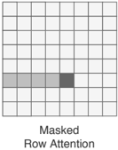<details> <summary>Image 8 Details</summary>  ### Visual Description ## Diagram: Masked Row Attention ### Overview The image displays a 7x7 grid visualization representing a "Masked Row Attention" mechanism, commonly used in Transformer-based machine learning models (such as GPT). The grid illustrates how a specific token in a sequence attends to previous tokens while being prevented from "seeing" future tokens. ### Components/Axes * **Grid Structure:** A 7x7 matrix of squares. * **Text Label:** Located directly below the grid, reading "Masked Row Attention." * **Visual Encoding:** * **White Squares:** Represent masked or ignored positions (future tokens). * **Light Gray Squares:** Represent attended positions (past tokens). * **Dark Gray Square:** Represents the current position (the query token). ### Detailed Analysis The diagram focuses on a single row (the 4th row from the top) to demonstrate the attention scope for a specific token. * **Grid Dimensions:** 7 columns by 7 rows. * **Active Row (Row 4):** * **Columns 1 through 4 (Left to Right):** Shaded in light gray. These represent the "past" context that the current token is allowed to attend to. * **Column 5:** Shaded in dark gray. This represents the current token position (the query). * **Columns 6 and 7:** Unshaded (white). These represent the "future" tokens, which are masked out to prevent information leakage during training. * **Inactive Rows:** All other rows (1-3 and 5-7) are entirely white, indicating that the diagram is isolating the attention behavior of a single token at a specific time step. ### Key Observations * **Asymmetry:** The shading is strictly left-aligned relative to the dark gray square, creating a triangular-like pattern of attention if this were applied to all rows. * **Causal Constraint:** The visual clearly demonstrates a "causal" constraint, where the model is restricted to looking backward in the sequence. * **Differentiation:** The use of two shades of gray (light vs. dark) distinguishes between the *context* (past tokens) and the *focus* (current token). ### Interpretation This diagram is a conceptual representation of **Causal Self-Attention** in Large Language Models (LLMs). * **Why it matters:** In autoregressive models, the goal is to predict the next token based on previous tokens. If the model were allowed to "see" the future tokens (the white squares to the right of the dark gray square) during training, it would simply copy the answer rather than learning to predict it. * **The "Mask":** The white squares represent the "mask" applied to the attention matrix. By setting the attention scores for these positions to negative infinity (before the Softmax function), the model effectively ignores them. * **Peircean Investigative Perspective:** * **The Sign:** The grid is an *icon* of the attention matrix. * **The Object:** The underlying mathematical operation is the masking of the upper-triangular portion of the attention matrix. * **The Interpretant:** The viewer understands this as a rule of sequence modeling: "You cannot know what comes next until you have processed what came before." The diagram serves as a visual proof of the model's inability to cheat during the training phase. 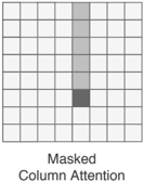</details> <details> <summary>Image 9 Details</summary>  ### Visual Description ## Diagram: Masked Column Attention ### Overview The image displays a 7x7 grid visualization representing a "Masked Column Attention" mechanism. It illustrates a specific attention pattern where only a single column is active, with varying degrees of shading applied to specific cells within that column. ### Components/Axes * **Grid Structure:** A 7x7 matrix of squares. * **Text Label:** "Masked Column Attention" positioned directly below the grid. * **Color/Shading Legend (Inferred):** * **White:** Unshaded/Inactive/Masked out. * **Light Gray:** Attended/Contextual region. * **Dark Gray:** The specific focus point or the "mask" anchor. ### Detailed Analysis The grid is organized into 7 rows and 7 columns. The attention pattern is isolated to the 5th column (counting from left to right). * **Columns 1, 2, 3, 4, 6, and 7:** All cells in these columns are white (unshaded). * **Column 5 (The Active Column):** * **Rows 1, 2, 3, and 4:** These four cells are filled with a light gray color. * **Row 5:** This cell is filled with a dark gray color. * **Rows 6 and 7:** These two cells are white (unshaded). ### Key Observations * **Vertical Isolation:** The attention mechanism is strictly vertical, affecting only one column out of the seven. * **Asymmetric Masking:** The shading is not uniform. There is a clear distinction between the light gray region (top four cells) and the dark gray cell (the fifth cell). * **Causal/Directional Flow:** The pattern suggests a directional dependency. The model attends to the four cells above the current position (Row 5), but ignores the two cells below it (Rows 6 and 7). ### Interpretation This diagram represents a **Masked Column Attention** mechanism, frequently used in Transformer-based architectures (such as those applied to image processing or specific sequence modeling). * **The Mechanism:** In this context, the dark gray square at Row 5, Column 5 likely represents the "query" or the current token/pixel being processed. * **The Context:** The light gray squares (Rows 1-4) represent the "key/value" pairs that the current position is allowed to attend to. This is a classic "causal" or "look-back" mask, where the model is restricted to seeing only the information that precedes the current position in a sequence or spatial scan. * **The Mask:** The white squares (Rows 6-7) represent the "future" or "masked" information that the model is prevented from seeing to avoid information leakage during training or inference. * **Significance:** This visualization demonstrates how a model maintains spatial awareness within a column while enforcing a strict directional constraint, ensuring that the prediction at any given point relies only on preceding data. 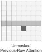</details> <details> <summary>Image 10 Details</summary>  ### Visual Description ## Diagram: Unmasked Previous-Row Attention Visualization ### Overview The image displays a 7x7 grid representing an attention mechanism matrix. It highlights specific patterns of connectivity between tokens or hidden states, labeled as "Unmasked Previous-Row Attention." ### Components/Axes * **Grid Structure:** A 7x7 square matrix. * **Text Label:** Located directly below the grid, reading: "Unmasked Previous-Row Attention". * **Visual Encoding (Color Legend):** * **White:** Represents no attention or masked connections. * **Light Gray:** Represents a row-wide attention connection. * **Dark Gray:** Represents a specific, localized attention connection. ### Detailed Analysis * **Grid Dimensions:** 7 rows by 7 columns. * **Row 4 (from top):** All 7 cells in this row are filled with light gray. This indicates that the attention mechanism is attending to the entire previous row simultaneously. * **Row 5 (from top):** Only the cell at Column 4 is filled with dark gray. This indicates a specific, point-to-point attention connection within the current row. * **Remaining Cells:** All other cells in the 7x7 grid are white, indicating no attention is being paid to those specific positions. ### Key Observations * **Asymmetry:** The pattern is not uniform. It combines a "global" row-level attention (the light gray horizontal band) with a "local" point-specific attention (the dark gray cell). * **Unmasked Nature:** The label "Unmasked" is significant. In standard Transformer architectures, attention is typically "masked" to prevent the model from looking at future tokens. This diagram illustrates a mechanism where that constraint is lifted for the previous row, allowing the model to access information from the entire previous row of hidden states. ### Interpretation This diagram is a schematic representation of a specific attention mechanism used in advanced neural network architectures, such as **Transformer-XL** or similar recurrent transformer models. * **Contextual Flow:** The "Previous-Row Attention" suggests that the model is processing data in segments or blocks. Instead of only attending to the current sequence, the model is designed to "look back" at the hidden states of the previous segment (the light gray row). * **Why it matters:** Standard Transformers have a fixed context window. By allowing "Unmasked" attention to the previous row, the model can maintain long-term dependencies across segment boundaries without needing to recompute the entire history. The dark gray cell likely represents the standard causal attention (attending to the current token or previous tokens in the current sequence), while the light gray row represents the recurrent memory mechanism. </details> (b) Combining two of the attention patterns, each position can attend to any of the previous positions, while not causing a state bottleneck as in fixed sparse attention (Child et al., 2019). 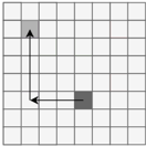<details> <summary>Image 11 Details</summary>  ### Visual Description ## Diagram: Grid Pathfinding Visualization ### Overview The image displays a 7x7 square grid containing two shaded cells and a directional path indicated by two arrows. The diagram illustrates a movement or relationship between two distinct points on a coordinate plane. There are no text labels, numbers, or legends present in the image. ### Components/Axes * **Grid Structure:** A 7x7 matrix composed of 49 equal-sized square cells. * **Shaded Cells:** * **Light Gray Square:** Located in the top-left quadrant of the grid. * **Dark Gray Square:** Located in the bottom-right quadrant of the grid. * **Arrows:** * **Horizontal Arrow:** A line segment with an arrowhead pointing left. * **Vertical Arrow:** A line segment with an arrowhead pointing up. ### Detailed Analysis To facilitate precise description, the grid is indexed using a 1-based coordinate system (Row, Column), where (1,1) is the top-left cell and (7,7) is the bottom-right cell. * **Grid Layout:** The grid consists of 7 rows and 7 columns. * **Positioning of Elements:** * **Light Gray Square:** Positioned at Row 2, Column 2. * **Dark Gray Square:** Positioned at Row 5, Column 5. * **Path Analysis:** * **Horizontal Segment:** The arrow originates at the center of the Dark Gray Square (5,5) and points left, terminating at the intersection of Row 5 and Column 3. * **Vertical Segment:** The arrow originates at the intersection of Row 5 and Column 3 (the "elbow" of the path) and points upward, terminating at the center of the Light Gray Square (2,2). * **Visual Trend:** The path describes a non-diagonal, rectilinear movement from the bottom-right shaded cell to the top-left shaded cell, moving first horizontally (left) and then vertically (up). ### Key Observations * **Rectilinear Movement:** The path strictly follows the grid lines, suggesting a constraint to orthogonal movement (up, down, left, right). * **Path Efficiency:** The path represents a "Manhattan distance" calculation, where the total distance is the sum of the absolute differences of the coordinates: |5-2| + |5-2| = 3 + 3 = 6 units of movement. * **Asymmetry:** The two shaded squares have different grayscale values, potentially indicating a hierarchy (e.g., Start vs. End, or Source vs. Destination). The darker square (5,5) acts as the source, and the lighter square (2,2) acts as the destination. ### Interpretation This diagram is a classic representation of **Manhattan Distance** (also known as Taxicab geometry) or a pathfinding algorithm visualization (such as A* or Dijkstra's algorithm) on a grid. * **What the data demonstrates:** It visualizes the concept that in a grid-based environment, the shortest path between two points is not a straight diagonal line, but a combination of horizontal and vertical steps. * **Peircean Investigative:** The use of arrows implies a temporal or causal sequence—a "flow" from the dark square to the light square. The "elbow" at (5,3) is a critical node, representing the point of decision where the path changes direction. * **Reading between the lines:** This image is likely a simplified model used in computer science or logistics to explain how agents (like robots or delivery vehicles) navigate a city grid or a digital matrix where diagonal movement is prohibited or impossible. The distinct shading suggests a clear distinction between the origin (darker) and the target (lighter). 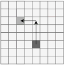</details> <details> <summary>Image 12 Details</summary>  ### Visual Description ## [Diagram]: Grid Path Visualization ### Overview The image displays a 7x7 square grid containing two distinct shaded cells connected by a directional path. The diagram illustrates a two-step movement pattern, likely representing a pathfinding algorithm, coordinate geometry, or a logic flow on a discrete grid. There is no text present in the image. ### Components/Axes * **Grid Structure:** A 7x7 matrix of equal-sized square cells. * **Start Point:** A dark gray square located at the intersection of the 5th row and 4th column (counting from the top-left as 1,1). * **End Point:** A light gray square located at the intersection of the 2nd row and 2nd column. * **Path Indicator:** A black arrow path originating from the center of the dark gray square, extending vertically upward, and turning 90 degrees to the left to terminate at the center of the light gray square. ### Detailed Analysis * **Grid Layout:** The grid is uniform, consisting of 49 total cells. * **Path Geometry:** * **Vertical Segment:** The path originates at (Row 5, Column 4) and travels vertically upward for 3 grid units, ending at (Row 2, Column 4). * **Horizontal Segment:** The path turns 90 degrees to the left at (Row 2, Column 4) and travels horizontally for 2 grid units, terminating at (Row 2, Column 2). * **Visual Hierarchy:** The start point is darker than the end point, suggesting a progression or a transition from a "source" state to a "destination" state. ### Key Observations * **Manhattan Distance:** The path represents the "Manhattan distance" (or taxicab geometry) between the two points, which is the sum of the absolute differences of their coordinates ($|5-2| + |4-2| = 3 + 2 = 5$ units). * **Movement Constraints:** The path implies a movement constraint where only vertical and horizontal movement is permitted (no diagonal movement). * **Directionality:** The arrowheads clearly define the sequence of movement: Vertical first, then Horizontal. ### Interpretation This diagram is a classic representation of pathfinding in a discrete 2D space. It demonstrates the shortest path between two points on a grid where diagonal movement is prohibited. * **Algorithmic Context:** This is a standard visualization for algorithms like A* (A-star) or Dijkstra’s algorithm, specifically in scenarios where the "cost" of movement is uniform across the grid. * **Logic Flow:** The transition from a darker shade to a lighter shade often signifies a "process" or "state change," where the darker cell represents the origin or current state, and the lighter cell represents the target or future state. * **Peircean Investigative Note:** The lack of labels suggests this is a generic instructional graphic intended to explain the *concept* of grid-based navigation rather than a specific dataset. The "L-shaped" path is the most efficient route, demonstrating the principle of least resistance in a constrained environment. 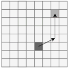</details> <details> <summary>Image 13 Details</summary>  ### Visual Description ## Diagram: Grid-Based Pathfinding Visualization ### Overview The image displays a 7x7 square grid containing two highlighted cells and a directional arrow indicating a path between them. This is a standard visual representation used in computer science and robotics to illustrate pathfinding algorithms or movement planning within a discrete environment. ### Components/Axes * **Grid Structure:** A 7x7 matrix of squares. * **Start Point:** A dark grey square located at coordinates (Row 5, Column 4), assuming a 1-based index starting from the top-left corner (1,1). * **End Point:** A light grey square located at coordinates (Row 2, Column 6). * **Path Indicator:** A two-segment arrow connecting the start and end points. ### Detailed Analysis The path is defined by two distinct segments: 1. **Segment 1:** Originates at the center of the dark grey square at (5, 4). The arrow extends diagonally upward and to the right, terminating at the center of the cell at (4, 5). 2. **Segment 2:** Originates at the center of the cell at (4, 5). The arrow extends vertically upward and slightly to the right, terminating at the center of the light grey square at (2, 6). ### Coordinate Mapping (Row, Column) | Point | Coordinates | Description | | :--- | :--- | :--- | | Start | (5, 4) | Dark Grey | | Intermediate Point | (4, 5) | N/A | | End | (2, 6) | Light Grey | ### Key Observations * **Non-Linear Path:** The path is not a straight line, indicating a deliberate change in direction at the intermediate point (4, 5). * **Movement Logic:** The path suggests a movement pattern that is not strictly Manhattan distance (which would require only horizontal and vertical moves) nor strictly diagonal. The first segment is diagonal, and the second segment is a steep diagonal/vertical hybrid. * **Visual Hierarchy:** The dark grey square acts as the origin (source), while the light grey square acts as the destination (target). ### Interpretation This diagram is a simplified model of **pathfinding or trajectory planning**. * **Context:** In a technical context, this likely represents an agent (the dark grey square) calculating a route to a goal (the light grey square) within a grid-based environment. * **Algorithmic Implication:** The bend in the arrow at (4, 5) suggests that the path was calculated to avoid an obstacle or to optimize for a specific cost function (e.g., minimizing distance or energy). Even though no obstacles are explicitly drawn, the deviation from a straight line implies that the "cost" of moving through the grid is not uniform, or that the movement rules of the agent are constrained (e.g., a robot that cannot move in a straight line to the target). * **Peircean Investigative Note:** The visual language is minimalist. The use of different shades of grey (dark vs. light) creates a clear hierarchy between the "source" and the "destination," allowing the viewer to immediately identify the direction of flow without needing labels. The arrow serves as the "interpretant," connecting the two states and defining the relationship between them as a sequence of actions. </details> Figure 6. Axis-aligned attention patterns sion completely without loss in training performance. For the Adam state tensors (m\_t, v\_t) we do dynamic scaling. For each iteration and for every parameter, we rescale its state tensors before casting so that their maximum corresponds to the maximum value of the float16 range, thus maximizing the use of the float16 range. Thus, we store the state m\_t as the tuple (scale, (m\_t/scale).half()) , where scale = m\_t.max()/float16.max() , and similarly for v\_t . The above lets us fit models of size 1 B parameters into memory for our large context of 8192 tokens. To train even larger models, we use GPipe (Huang et al., 2019b). ## B. Experimental details ## B.1. Music VQ-VAE We have three separate raw audio VQ-VAEs to produce discrete codes at varying hop sizes for the bottom, middle, and top priors. All autoencoders comprise non-causal, dilated 1-D convolutions, and are trained independently using nonautoregressive reconstruction losses. Basic building blocks in these networks share the same architecture, as shown in Figure 7. Each encoder block consists of a downsampling convolution, a residual network, and a 1D convolution with a kernel size of 3. Dilation is grown by a factor of 3 in these residual networks to increase the receptive field. The decoder block mirrors this exactly with a 1D convolution with the kernel size of 3, a residual network with dilation contracting across depth, and an upsampling transposed convolution. Here, all resampling convolutions use a kernel size of 4 and stride 2 so that each building block changes the hop length by a factor of 2. To get higher compression in time, we simply stack more of these blocks. For example, using seven blocks yields a hop length of 128 for the top level autoencoder. Each residual network has four residual blocks in the middle and top VQ-VAEs resulting in a receptive field of 120 ms and 480 ms for the respective discrete tokens. Because increasing the residual depth helped improve reconstruction quality slightly, we doubled the number of residual blocks for the bottom level. This dramatically increases the receptive field to about 2 seconds per code but the actual receptive field is mostly local. We also experimented with having a single decoder and modeling the residuals to separate out learned representations as in (Razavi et al., 2019), hoping upsampling priors would simply fill in local musical structure. However, pushing information to the top level was quite challenging as the bottommost level reconstructs almost perfectly early on in training. When we add auxiliary objectives to encourage the top to be used more, the top-level codes add serious distortions to the final output. A similar challenge is shown in (Dieleman et al., 2018). ## B.2. Music Priors and Upsamplers Architectural details of our music prior and upsampler models are depicted in Figure 8. They perform autoregressive modeling of tokens at each level, conditioned on information such as artist and genre, as well as the tokens from the upper level in the case of the upsamplers (Figure 8a). Each artist and genre are learned as embedding vectors, whose sum is provided as the very first token in each sequence. In addition, positional embedding is learned as a function of each position's absolute and relative timing in the duration of the song. 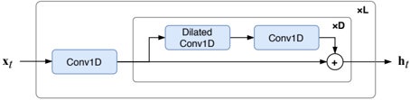In upsampler models, upper-level tokens <details> <summary>Image 14 Details</summary>  ### Visual Description ## Diagram: Neural Network Block Architecture ### Overview The image illustrates a modular neural network architecture block, commonly used in sequence modeling (such as WaveNet or Temporal Convolutional Networks). The diagram depicts a signal flow that incorporates an initial convolution, a residual branch containing a dilated convolution, and a summation operation. The structure is nested, indicating that specific components are repeated $D$ times and the entire block is repeated $L$ times. ### Components/Axes * **Input/Output:** * **$x_t$**: The input signal, entering from the left. * **$h_t$**: The output signal, exiting to the right. * **Processing Blocks (Blue Rectangles):** * **Conv1D (Left):** The initial 1D convolution layer. * **Dilated Conv1D (Top-Center):** A 1D convolution layer with dilation, located inside the inner box. * **Conv1D (Top-Right):** A standard 1D convolution layer, located inside the inner box, following the Dilated Conv1D. * **Operations:** * **$\oplus$ (Summation Node):** Located on the right side, this node adds the output of the processing path to the residual path. * **Containers/Multipliers:** * **Inner Box (labeled "xD"):** Encloses the "Dilated Conv1D" and the second "Conv1D" block. This indicates that this specific sequence of operations is repeated $D$ times. * **Outer Box (labeled "xL"):** Encloses the entire architecture, including the initial "Conv1D" and the "xD" box. This indicates that the entire block structure is repeated $L$ times. ### Detailed Analysis The flow of data through the diagram is as follows: 1. **Initial Processing:** The input $x_t$ enters the first "Conv1D" block. 2. **Branching:** Upon exiting the first "Conv1D" block, the signal path splits: * **Residual Path (Bottom):** A direct, horizontal line connects the output of the first "Conv1D" directly to the summation node ($\oplus$). This is a "skip connection." * **Processing Path (Top):** The signal enters the inner box ("xD"). It passes through the "Dilated Conv1D" block, then flows into the second "Conv1D" block. 3. **Recombination:** The output of the processing path (from the second "Conv1D") is directed downward into the summation node ($\oplus$), where it is added to the signal from the residual path. 4. **Output:** The result of the summation is the output $h_t$. ### Key Observations * **Residual Learning:** The presence of the direct line bypassing the "Dilated Conv1D" and "Conv1D" blocks indicates a residual connection, which is a standard technique to facilitate the training of deeper networks by allowing gradients to flow more easily. * **Receptive Field Expansion:** The use of "Dilated Conv1D" suggests the architecture is designed to increase the receptive field of the network (the amount of input data the network "sees" at once) without significantly increasing the number of parameters. * **Scalability:** The labels "xD" and "xL" explicitly define the scalability of the architecture. The network depth can be adjusted by changing $L$, and the complexity of the dilated processing can be adjusted by changing $D$. ### Interpretation This diagram represents a fundamental building block for deep temporal models. The architecture is designed to process sequential data ($x_t$) while maintaining the ability to learn long-range dependencies. The "Dilated Conv1D" is the critical component here; by skipping input values (dilation), the network can capture patterns over a longer time horizon than a standard convolution would allow with the same kernel size. The residual connection (the skip connection) is essential for the "xL" scaling—without it, stacking many layers (large $L$) would likely lead to vanishing gradients, making the model impossible to train. The structure suggests a highly efficient, hierarchical feature extractor where the model learns to combine local features (via the initial Conv1D) with broader temporal context (via the Dilated Conv1D). </details> (a) The encoder compresses the raw audio input into a sequence of embeddings. The length of this latent representation relative to the raw audio duration determines the amount of compression, and is an important factor for the trade-off between fidelity and coherence. 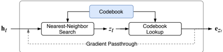<details> <summary>Image 15 Details</summary>  ### Visual Description ## Diagram: Vector Quantization Process Flow ### Overview The image is a schematic flow diagram illustrating the architecture of a Vector Quantization (VQ) layer, commonly used in machine learning models such as VQ-VAEs (Vector Quantized Variational Autoencoders). The diagram visualizes the forward pass of an input vector through a quantization process and the backward pass mechanism known as "Gradient Passthrough." ### Components/Axes The diagram is contained within a large, rounded rectangular bounding box. The components are arranged as follows: * **Input:** $\mathbf{h}_t$ (located at the far left). * **Processing Blocks:** * **Nearest-Neighbor Search:** A rectangular box located in the center-left. * **Codebook Lookup:** A rectangular box located in the center-right. * **Reference Component:** * **Codebook:** A blue-shaded rectangular box positioned at the top-center, connected to both processing blocks. * **Intermediate Variable:** $z_t$ (located on the arrow between the two processing blocks). * **Output:** $\mathbf{e}_{z_t}$ (located at the far right). * **Feedback Mechanism:** * **Gradient Passthrough:** A dashed line originating from the output $\mathbf{e}_{z_t}$ and looping back to the input $\mathbf{h}_t$. ### Detailed Analysis The flow of information proceeds as follows: 1. **Forward Pass:** * The input vector $\mathbf{h}_t$ enters the "Nearest-Neighbor Search" block. * The "Codebook" (blue box) provides reference data to the "Nearest-Neighbor Search" block to determine the closest match. * The result of this search is $z_t$, which represents the index or identifier of the nearest neighbor. * $z_t$ is passed to the "Codebook Lookup" block. * The "Codebook" also provides data to the "Codebook Lookup" block. * The "Codebook Lookup" block retrieves the actual vector $\mathbf{e}_{z_t}$ corresponding to the index $z_t$. * The final output is $\mathbf{e}_{z_t}$. 2. **Backward Pass (Gradient Flow):** * A dashed line labeled "Gradient Passthrough" connects the output $\mathbf{e}_{z_t}$ back to the input $\mathbf{h}_t$. This indicates that during backpropagation, the gradient is copied directly from the output to the input, bypassing the non-differentiable quantization operation. ### Key Observations * **Shared Resource:** The "Codebook" is positioned centrally above the processing chain, indicating it is a shared memory or lookup table accessed by both the search and lookup operations. * **Non-Differentiable Operation:** The distinction between the solid lines (forward pass) and the dashed line (gradient passthrough) highlights the architectural solution to the non-differentiability of the nearest-neighbor search. * **Modular Design:** The entire process is enclosed in a bounding box, suggesting this is a discrete, modular unit within a larger neural network architecture. ### Interpretation This diagram represents the core mechanism of Vector Quantization. The "Nearest-Neighbor Search" is a discrete operation (finding the closest vector in a codebook), which is mathematically non-differentiable. Because standard neural network training relies on backpropagation (calculus-based gradient descent), this operation would normally "break" the training process. The "Gradient Passthrough" is the critical component here. By treating the quantization operation as an identity mapping during the backward pass (copying the gradient from $\mathbf{e}_{z_t}$ directly to $\mathbf{h}_t$), the model allows the encoder (which produces $\mathbf{h}_t$) to learn how to produce vectors that are closer to the codebook entries, even though the forward pass involves a discrete selection. This allows the entire system to be trained end-to-end. </details> (b) The bottleneck takes the sequence of embeddings from the encoder and maps it into a sequence of code vectors from the codebook. This sequence of code indices is used as a discrete representation to be modeled by the priors. Larger codebooks improve fidelity but may be more difficult to compress. 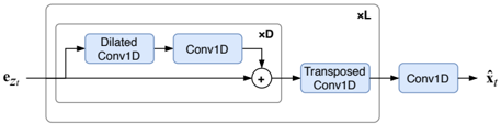<details> <summary>Image 16 Details</summary>  ### Visual Description ## Diagram: Neural Network Architecture Block ### Overview The image displays a block diagram representing a neural network architecture, likely a decoder or generator component used for processing sequential data (such as audio or time-series). The flow moves from left to right, transforming an input signal $e_{Z_t}$ into an output signal $\hat{x}_t$ through a series of convolutional operations, including a residual block structure. ### Components/Axes * **Input:** $e_{Z_t}$ (located at the far left). * **Output:** $\hat{x}_t$ (located at the far right). * **Processing Blocks (Light Blue Rectangles):** * **Dilated Conv1D:** A convolutional layer with dilation. * **Conv1D:** A standard 1D convolutional layer. * **Transposed Conv1D:** A 1D transposed convolutional layer (often used for upsampling). * **Conv1D:** A final standard 1D convolutional layer. * **Structural Containers:** * **xD:** An inner box containing the residual block (Dilated Conv1D and Conv1D). The "xD" label indicates this block is repeated $D$ times. * **xL:** An outer box containing the "xD" block and the "Transposed Conv1D" layer. The "xL" label indicates this entire structure is repeated $L$ times. * **Operators:** * **$\oplus$ (Addition):** A circle containing a plus sign, representing a residual (skip) connection summation. ### Detailed Analysis The diagram follows a sequential flow from left to right: 1. **Input Stage:** The signal $e_{Z_t}$ enters the system. 2. **Residual Block (Inner 'xD' container):** * The input signal splits into two paths. * **Upper Path:** The signal passes through a "Dilated Conv1D" layer, followed by a "Conv1D" layer. * **Lower Path:** The signal bypasses the convolutional layers (a skip connection). * **Merge:** The outputs of the upper and lower paths are combined at the addition operator ($\oplus$). 3. **Upsampling/Transformation (Outer 'xL' container):** * The output from the residual block enters a "Transposed Conv1D" layer. 4. **Final Output Stage:** * After exiting the "xL" container, the signal passes through a final "Conv1D" layer. * The process terminates at the output $\hat{x}_t$. ### Key Observations * **Residual Connection:** The presence of the $\oplus$ operator indicates a residual architecture, which is commonly used to mitigate vanishing gradient problems in deep networks. * **Dilated Convolution:** The use of "Dilated Conv1D" suggests the model is designed to capture long-range dependencies or a wider receptive field without significantly increasing the number of parameters. * **Hierarchical Structure:** The nesting of "xD" inside "xL" implies a hierarchical design where a specific residual block is repeated $D$ times, and that entire sequence is then repeated $L$ times, likely to increase the depth and representational capacity of the model. * **Upsampling:** The "Transposed Conv1D" layer suggests that the model is increasing the temporal resolution of the data as it passes through the "xL" blocks. ### Interpretation This diagram represents a standard architecture for generative models, such as those used in speech synthesis (e.g., WaveNet-style vocoders) or time-series forecasting. * **Data Flow:** The architecture takes a latent representation ($e_{Z_t}$) and progressively refines it. * **Functionality:** The "xD" block acts as a feature extractor that preserves information via the skip connection while learning complex patterns via the dilated convolutions. The "Transposed Conv1D" layer serves to expand the signal, likely increasing the sampling rate or temporal length. * **Peircean Investigative Note:** The notation "xD" and "xL" are standard shorthand in deep learning literature for "repeat $D$ times" and "repeat $L$ times." This indicates that the diagram is a simplified representation of a much deeper network. The final "Conv1D" layer acts as a projection head, mapping the high-level features learned by the "xL" blocks into the final output space $\hat{x}_t$. </details> (c) The decoder reconstructs the raw audio from latent representations. It is a mirror of the encoder where dilations constracts by a factor of 3 down to 1 at the last block. The final Conv1D projects to the desired number of audio channels and also acts as a smoothing operation after a sequence of transposed convolutions. Figure 7. Components of the VQ-VAE model are upsampled by the conditioner network, using WaveNetstyle dilated convolutions followed by a transposed 1-D convolutional layer (Figure 8b). When the model is trained on lyrics, the top-level prior takes lyrics data corresponding to each audio segment and uses them to train an encoder-decoder Transformer as shown in Figure 8c. All transformer stacks use sparse self-attention layers with the three factorized attention types (row, column, and previous-row) repeating, and encoder-decoder attention layers, when present, are interleaved with the other attention types. Each layer consists of residual connections of an attention and an MLP feedforward network, each prepended by layer normalization (see Figure 8d). 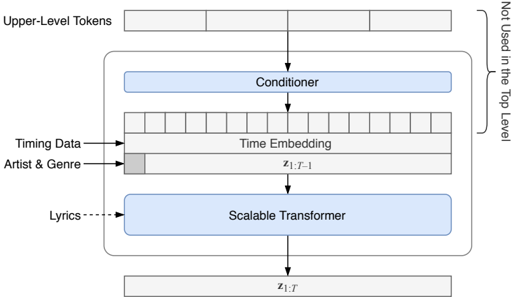<details> <summary>Image 17 Details</summary>  ### Visual Description ## Diagram: Hierarchical Transformer Architecture for Audio/Music Generation ### Overview This diagram illustrates the architecture of a neural network, likely a hierarchical transformer model designed for music or audio generation. The flow is top-down, showing how upper-level tokens and various conditioning inputs (Artist, Genre, Lyrics, Timing) are processed through a "Scalable Transformer" to produce a final sequence of tokens ($z_{1:T}$). ### Components/Axes The diagram is organized into a vertical stack enclosed within a main rounded rectangular container, with additional annotations on the periphery. **Main Components (Top to Bottom):** * **Upper-Level Tokens:** A row of four empty rectangular boxes at the very top. * **Conditioner:** A blue rectangular block located below the Upper-Level Tokens. * **Time Embedding:** A row of 12 small, light-grey boxes positioned above a horizontal bar. * **$z_{1:T-1}$:** A horizontal bar representing the input sequence. On the far left of this bar is a small, shaded grey box. * **Scalable Transformer:** A large blue rectangular block located below the $z_{1:T-1}$ bar. * **$z_{1:T}$:** A horizontal bar at the bottom of the diagram, representing the final output sequence. **Annotations and Labels:** * **Right Side:** A large curly bracket spans the "Conditioner," "Time Embedding," and "$z_{1:T-1}$" blocks, labeled "Not Used in the Top Level." * **Left Side (Arrows):** * **Timing Data:** A solid arrow pointing to the "Time Embedding" row. * **Artist & Genre:** A solid arrow pointing to the small grey box on the left side of the $z_{1:T-1}$ bar. * **Lyrics:** A dashed arrow pointing directly into the "Scalable Transformer" block. ### Detailed Analysis The diagram depicts a sequential data processing pipeline: 1. **Input Flow:** The process begins with "Upper-Level Tokens," which pass through a "Conditioner." 2. **Conditioning:** The output of the Conditioner influences the "Time Embedding" and the sequence $z_{1:T-1}$. 3. **Sequence Integration:** * The "Time Embedding" provides temporal context. * The $z_{1:T-1}$ bar represents the autoregressive input (the sequence generated so far). * The small grey box within $z_{1:T-1}$ explicitly injects "Artist & Genre" information into the sequence. 4. **Transformation:** The "Scalable Transformer" acts as the primary processing engine. It takes the conditioned sequence ($z_{1:T-1}$) and integrates "Lyrics" (via the dashed arrow) to perform the computation. 5. **Output:** The transformer outputs the final sequence $z_{1:T}$. ### Key Observations * **Hierarchical Nature:** The bracket on the right labeled "Not Used in the Top Level" strongly implies this is a sub-module of a larger, hierarchical system. The "Top Level" likely operates on a coarser resolution, while this module operates on a finer resolution. * **Multi-Modal Conditioning:** The model is highly conditioned. It integrates global context (Upper-Level Tokens), temporal context (Time Embedding), metadata (Artist & Genre), and semantic content (Lyrics). * **Autoregressive Structure:** The notation $z_{1:T-1}$ as input and $z_{1:T}$ as output is characteristic of autoregressive models, where the model predicts the next token in a sequence based on all previous tokens. ### Interpretation This architecture represents a sophisticated generative model, likely used for tasks such as singing voice synthesis or music generation with lyrics. * **The Role of the Conditioner:** The Conditioner serves as a bridge, translating the abstract, high-level representations ("Upper-Level Tokens") into a format that the lower-level Transformer can utilize. * **The Role of the Transformer:** By receiving both the previous sequence ($z_{1:T-1}$) and the lyrics, the "Scalable Transformer" is tasked with aligning the semantic content (lyrics) with the temporal and stylistic constraints (Artist, Genre, Timing) to generate the next segment of audio/music. * **Peircean Investigative Note:** The dashed arrow for "Lyrics" versus the solid arrows for other inputs suggests that the lyrics might be injected as a cross-attention mechanism or a separate conditioning input, rather than being part of the primary sequence embedding, distinguishing semantic content from the structural/temporal sequence. </details> - (a) The structure of our prior models, performing next-token prediction at each level. The Transformer takes the embeddings of the tokens z 1: T -1 prepended by the sum of the artist and genre embeddings, in addition to the time embedding that encodes relative and absolute timing of the segments in the duration of the song. The upsampler priors additionally take the tokens from the upper level, which are fed to the conditioner network and added to the input sequence. The top-level prior takes lyrics as conditioning information as well (see Figure 8c). Token Embedding + Transposed Conv1D - (b) The conditioner network takes the tokens from the upper level, and their embedding vectors go through non-causal WaveNet-like layers with increasingly dilated convolutions. The transposed 1-D convolution upsamples the sequence to the higher temporal resolution of the current level. - (d) Each Transformer layer is a residual attention block, which performs two residual operations, attention and MLP, each prepended with layer normalization. Depending on the layer's type, it uses either one of the three factorized attentions or encoder-decoder attention taking the lyrics features from the encoder. (c) The Scalable Transformer architecture, shown with the lyrics Transformer used in the top-level prior. The Transformer layers use the three factorized attention types alternatingly, i.e. repeating row, column, and previous-row attentions. In the top-level prior, the VQ Transformer additionally includes interleaved encoder-decoder attention layers that apply lyrics conditioning by attending on the activation of the last encoder layer. 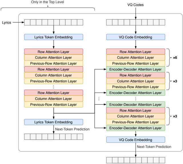<details> <summary>Image 18 Details</summary>  ### Visual Description ## Diagram: Neural Network Architecture for Lyrics and VQ Codes ### Overview The image displays a dual-stream neural network architecture designed for sequence generation, likely for music or audio synthesis. The architecture consists of two parallel processing streams: a "Lyrics" stream on the left and a "VQ Codes" (Vector Quantized Codes) stream on the right. The entire structure is enclosed within a bracket labeled "Only in the Top Level," suggesting this is a component of a larger, hierarchical model. The two streams interact via cross-attention mechanisms, allowing the VQ Code stream to condition its output on the Lyrics stream. ### Components/Axes The diagram uses a color-coded system to represent different types of neural network layers: * **Blue:** Embedding layers ("Lyrics Token Embedding", "VQ Code Embedding"). * **Red:** "Row Attention Layer". * **Orange:** "Column Attention Layer". * **Yellow:** "Previous-Row Attention Layer". * **Green:** "Encoder-Decoder Attention Layer". **Structural Elements:** * **Input/Output:** Represented by arrays of empty boxes at the top and bottom of each stream. * **Flow:** Indicated by vertical arrows connecting the layers. * **Multipliers:** Annotations like "x6" and "x3" indicate the repetition of specific layer blocks. * **Cross-Connection:** A horizontal arrow connects the output of the first set of attention layers in the Lyrics stream to the Encoder-Decoder layers in the VQ Codes stream. ### Detailed Analysis #### Left Stream (Lyrics) * **Input:** Starts with an input array labeled "Lyrics". * **Embedding:** Passes through a "Lyrics Token Embedding" layer. * **Processing Blocks:** A repeating sequence of [Row Attention Layer, Column Attention Layer, Previous-Row Attention Layer]. * **Output:** The stream concludes with a "Lyrics Token Embedding" layer, followed by a "Next-Token Prediction" step, leading to an output array. * **Connection:** A branch line exits the stream after the first set of attention layers and connects to the right stream. #### Right Stream (VQ Codes) * **Input:** Starts with an input array labeled "VQ Codes". * **Embedding:** Passes through a "VQ Code Embedding" layer. * **Top Block:** A stack of [Row Attention Layer, Column Attention Layer, Previous-Row Attention Layer] repeated **x6** times. * **Middle/Bottom Blocks:** * The stream incorporates "Encoder-Decoder Attention Layer" blocks. * The structure follows a pattern: [Encoder-Decoder Attention Layer] -> [Row, Column, Previous-Row] (repeated **x3** times) -> [Encoder-Decoder Attention Layer]. * An ellipsis (...) indicates this pattern repeats. * The bottom section mirrors the middle: [Encoder-Decoder Attention Layer] -> [Row, Column, Previous-Row] (repeated **x3** times) -> [Encoder-Decoder Attention Layer]. * **Output:** Concludes with a "VQ Code Embedding" layer, followed by a "Next-Token Prediction" step, leading to an output array. ### Key Observations * **Asymmetry:** The Lyrics stream is significantly simpler and lacks the Encoder-Decoder layers found in the VQ Codes stream. * **Conditioning:** The VQ Codes stream is the primary generator, which is conditioned on the Lyrics stream via the Encoder-Decoder Attention Layers. * **Hierarchical Attention:** The use of "Row," "Column," and "Previous-Row" attention layers suggests the model is processing data that has a 2D structure (like a spectrogram or a grid of audio tokens), allowing the model to attend to spatial relationships within the data. * **Repetition:** The "x6" and "x3" multipliers indicate a deep architecture, likely a Transformer-based variant designed to handle long-range dependencies in audio generation. ### Interpretation This architecture represents a conditional generative model. The "Lyrics" stream acts as an encoder that processes textual input, while the "VQ Codes" stream acts as a decoder that generates audio tokens (VQ codes). The "Encoder-Decoder Attention Layers" in the right stream are the critical interface; they allow the model to align the generated audio tokens with the specific lyrics provided. The "Row," "Column," and "Previous-Row" attention layers suggest that the VQ codes are arranged in a grid (likely representing time and frequency or temporal chunks), and the model uses these specific attention mechanisms to capture the structure of the audio signal effectively. The "Only in the Top Level" label implies that this diagram describes a specific stage of a multi-stage generation process, where this module is responsible for high-level or final-stage synthesis. 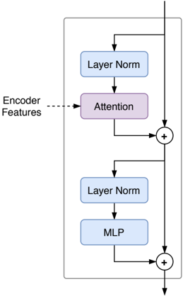</details> <details> <summary>Image 19 Details</summary>  ### Visual Description ## Diagram: Neural Network Block Architecture ### Overview The image displays a schematic block diagram of a neural network layer, characteristic of a Transformer decoder block. The diagram illustrates a sequential data flow through normalization, attention, and feed-forward (MLP) layers, incorporating residual connections (skip connections) at two distinct stages. ### Components/Flow The diagram is enclosed within a large rectangular container. The flow is primarily top-to-bottom. **Top Section (Attention Mechanism):** * **Input:** Data enters from the top of the container. * **Layer Norm:** A light blue rectangular block labeled "Layer Norm" processes the input. * **Attention:** A light purple rectangular block labeled "Attention" follows the first Layer Norm. * **External Input:** A dashed arrow points from the left, labeled "Encoder Features," indicating an external input into the "Attention" block. * **Residual Connection:** A vertical line runs down the right side of the container. At the output of the "Attention" block, this line meets the block's output at a circle containing a "+" symbol, indicating a summation (residual addition). **Bottom Section (Feed-Forward Mechanism):** * **Layer Norm:** The output from the first summation flows into a second light blue rectangular block labeled "Layer Norm." * **MLP:** This flows into a light blue rectangular block labeled "MLP" (Multi-Layer Perceptron). * **Residual Connection:** The vertical line on the right continues downward. At the output of the "MLP" block, it meets the block's output at a second circle containing a "+" symbol, indicating a second summation. * **Output:** The final result exits the container at the bottom. ### Detailed Analysis * **Color Coding:** * **Light Blue:** Used for "Layer Norm" and "MLP" blocks, representing standard processing layers. * **Light Purple:** Used for the "Attention" block, highlighting its distinct role compared to the other components. * **Structural Logic:** * The diagram follows a standard "Add & Norm" pattern common in deep learning architectures. * The presence of the "Encoder Features" input specifically identifies this as a **Cross-Attention** layer within a Transformer decoder. * The vertical line on the right acts as a "highway" for the residual connection, allowing the original input to bypass the transformation layers and be added back to the processed output. ### Key Observations * **Sequential Dependency:** The architecture is strictly sequential; the output of the top section (Attention) is the input for the bottom section (MLP). * **Residual Integration:** There are two distinct residual connections. The first bypasses the Layer Norm and Attention mechanism. The second bypasses the Layer Norm and MLP mechanism. * **External Dependency:** The "Attention" block is the only component that accepts an external input ("Encoder Features"), distinguishing it from the self-contained nature of the "MLP" block. ### Interpretation This diagram represents a **Transformer Decoder Cross-Attention Block**. * **Functionality:** The data flow demonstrates how a decoder integrates information from an encoder. The "Attention" block allows the decoder to focus on specific parts of the encoder's output (the "Encoder Features") relative to the current sequence being processed. * **Why it matters:** The residual connections (the "+" circles) are critical for training deep neural networks. They mitigate the "vanishing gradient" problem by providing a direct path for gradients to flow backward through the network during training, allowing for the construction of much deeper models. * **Peircean Investigative Note:** The visual distinction of the "Attention" block (purple) versus the "MLP" block (blue) suggests a functional separation: the purple block is dynamic and context-dependent (based on external encoder features), while the blue blocks are static, learned transformations applied to the data. The structure implies that the model first aligns its internal state with external information (Attention) and then refines that information through a feed-forward network (MLP). </details> Figure 8. Detailed architecture of the music prior and upsampler models Dilated Conv1D Conv1D ×D ## B.3. Hyperparameters For all Transformers' residual blocks, we use MLP blocks with the same width as the model width, and attention blocks with queries, keys, and values with width 0.25 times the model width. For all convolutional residual blocks, we use convolutions with same channels as the model width. | Sample rate | 44100 | |-------------------------------------|-----------------| | Sample length | 393216 | | Hop lengths | 8, 32, 128 | | Embedding width | 64 | | Residual block width | 64, 32, 32 | | Residual blocks (per 2x downsample) | 8, 4, 4 | | Conv filter size | 3 | | Conv channels | 32 | | Dilation growth rate | 3 | | Commit weight β | 0.02 | | Codebook EMA γ | 0.99 | | Codebook size | 2048 | | Spectral loss STFT bins | 2048, 1024, 512 | | Spectral loss STFT hop length | 240, 120, 50 | | Spectral loss STFT window size | 1200, 600, 240 | | Initialization scale | 0.02 | | Batch size | 256 | | Training steps | 384618 | | Learning rate | 0.0003 | Table 4. VQ-VAE hyperparameters | | 1B upsamplers | |----------------------------------|-----------------| | Sample length | 262144, 65536 | | Context length | 8192 | | Transformer width | 1920 | | Transformer layers | 72 | | Attention heads | 1 | | Factorized attention shape | (128, 64) | | Conditioner residual block width | 1024 | | Conditioner residual blocks | 16 | | Conditioner conv filter size | 3 | | Conditioner conv channels | 1024 | | Conditioner dilation growth rate | 3 | | Conditioner dilation cycle | 8 | | Initialization scale | 0.004, 0.008 | | Batch size | 192, 184 | | Training steps | 265000, 279000 | | Learning rate | 0.0003 | | Adam β 2 | 0.95 | | Weight decay | 0.01 | Table 5. Middle- and bottom-level upsampler hyperparameters Table 6. Top-level prior hyperparameters | | 5B prior | |-----------------------------------------|------------| | Sample length | 1048576 | | Context length | 8192 | | Transformer width | 4800 | | Transformer self-attention layers | 72 | | Attention heads | 8 | | Factorized attention shape | (128, 64) | | Lyrics encoder tokens | 512 | | Lyrics encoder width | 1280 | | Lyrics encoder layers | 18 | | Lyrics encoder attention heads | 4 | | Lyrics encoder factored attention shape | (32, 16) | | Encoder-Decoder attention layers | 7 | | Initialization scale | 0.002 | | Encoder initialization scale | 0.014 | | Batch size | 512 | | Training steps | 310500 | | Learning rate | 0.00015 | | Adam β 2 | 0.925 | | Weight decay | 0.002 | ## B.4. t -SNE Plot of Artists Figure 9. t -SNE of (artist, genre) embedding. The overall clustering shows very clearly how genres are related to one another. The broadest of all, pop, is situated in the middle of rock, country, blues, hip hop, and many more. Soundtrack and classical form their own island. Within a genre, we see a similar trend among artists. John Lennon, Paul McCartney, George Harrison and Ringo Starr are clustered around The Beatles. Cheap Trick which has a number of Beatles covers is also found near. Because we are showing only about 400 artists here, not all neighboring artists may be related. For an interactive version, we point to our blog post. 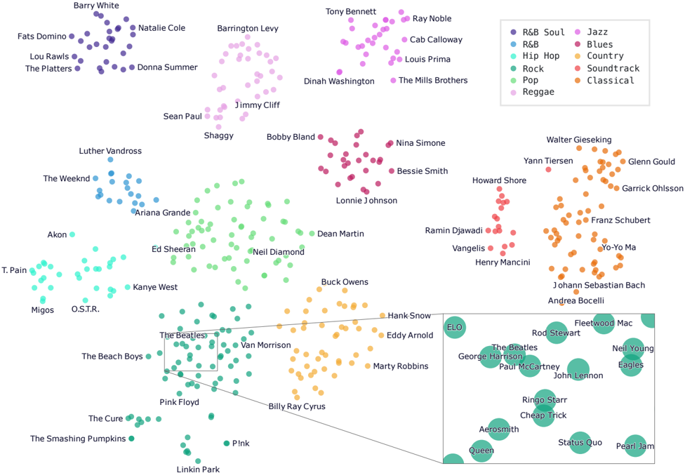<details> <summary>Image 20 Details</summary>  ### Visual Description ## Scatter Plot: Musical Artist Genre Clustering ### Overview The image is a two-dimensional scatter plot visualizing the relationships between various musical artists based on genre similarity. The plot uses color-coded clusters to represent ten distinct musical genres. A zoomed-in inset box at the bottom right provides a detailed view of the "Rock" cluster, highlighting specific artists within that group. ### Components/Axes * **Axes:** The plot does not have labeled axes, which is characteristic of dimensionality reduction visualizations (such as t-SNE or UMAP), where the X and Y coordinates represent relative similarity rather than specific quantitative metrics. * **Legend (Top Right):** * **R&B Soul:** Purple * **R&B:** Blue * **Hip Hop:** Teal * **Rock:** Green * **Reggae:** Light Purple * **Jazz:** Light Pink * **Blues:** Dark Pink * **Country:** Yellow/Orange * **Soundtrack:** Red * **Classical:** Orange * **Inset (Bottom Right):** A rectangular callout box magnifying a dense region of the "Rock" (Green) cluster. ### Detailed Analysis #### Cluster Distribution * **Top-Left (Purple - R&B Soul):** Contains Barry White, Natalie Cole, Fats Domino, Lou Rawls, The Platters, and Donna Summer. * **Top-Middle (Light Purple - Reggae):** Contains Barrington Levy, Sean Paul, Jimmy Cliff, and Shaggy. * **Top-Middle (Light Pink - Jazz):** Contains Tony Bennett, Ray Noble, Cab Calloway, Louis Prima, Dinah Washington, and The Mills Brothers. * **Middle-Left (Blue - R&B):** Contains Luther Vandross, The Weeknd, Ariana Grande, Akon, T. Pain, Migos, and O.S.T.R. * **Center/Bottom (Green - Rock):** A large, sprawling cluster containing Ed Sheeran, Neil Diamond, Dean Martin, The Beatles, Van Morrison, The Beach Boys, Pink Floyd, The Cure, The Smashing Pumpkins, P!nk, and Linkin Park. * **Middle (Dark Pink - Blues):** Contains Bobby Bland, Nina Simone, Bessie Smith, and Lonnie Johnson. * **Right (Red - Soundtrack):** Contains Howard Shore, Ramin Djawadi, Vangelis, and Henry Mancini. * **Right (Orange - Classical):** Contains Walter Gieseking, Yann Tiersen, Glenn Gould, Garrick Ohlsson, Franz Schubert, Yo-Yo Ma, Johann Sebastian Bach, and Andrea Bocelli. * **Bottom-Middle (Yellow/Orange - Country):** Contains Buck Owens, Hank Snow, Eddy Arnold, Marty Robbins, and Billy Ray Cyrus. #### Inset Analysis (Bottom Right) The inset provides a magnified view of the "Rock" cluster. It reveals that the model distinguishes between individual members of bands and the bands themselves. * **Artists/Bands identified:** ELO, Rod Stewart, Fleetwood Mac, Neil Young, Eagles, George Harrison, Paul McCartney, John Lennon, The Beatles, Ringo Starr, Cheap Trick, Aerosmith, Queen, Status Quo, Pearl Jam. ### Key Observations * **Genre Proximity:** The spatial arrangement reflects musical lineage. For example, the "Soundtrack" (Red) cluster is positioned directly adjacent to the "Classical" (Orange) cluster, likely due to shared orchestral instrumentation. Similarly, "R&B" (Blue) and "Hip Hop" (Teal) are clustered closely together. * **Granularity:** The inclusion of individual Beatles members (John Lennon, Paul McCartney, George Harrison, Ringo Starr) alongside the band "The Beatles" suggests the underlying data model is sensitive to individual artist discography versus group discography. * **Outliers:** Some placements are unconventional based on traditional genre definitions. For example, Dean Martin is placed within the "Rock" cluster, despite being primarily known for traditional pop and jazz standards. This suggests the model may be clustering based on specific features (e.g., production era, popularity, or collaborative networks) rather than strict genre labels. ### Interpretation This visualization is a classic example of a dimensionality reduction technique (likely t-SNE) applied to music metadata. The data demonstrates that musical genres are not isolated silos but exist on a continuous spectrum of similarity. The "gravity" of the clusters suggests that artists are positioned based on the "distance" between their musical styles. The proximity of the "Classical" and "Soundtrack" clusters indicates a high degree of overlap in their acoustic profiles. The inset highlights the model's ability to resolve high-density areas, showing that it can differentiate between the collective output of a band and the solo careers of its members, placing them in close proximity but as distinct data points. This suggests the model is likely trained on features derived from audio analysis or collaborative filtering (user listening habits) rather than manually assigned genre tags. </details>