## TOWARDS INTERVENTION-CENTRIC CAUSAL REASONING IN LEARNING AGENTS
Benjamin Lansdell Department of Bioengineering University of Pennsylvania Philadelphia, PA
## ABSTRACT
Interventions are central to causal learning and reasoning. Yet ultimately an intervention is an abstraction: an agent embedded in a physical environment (perhaps modeled as a Markov decision process) does not typically come equipped with the notion of an intervention - its action space is typically ego-centric, without actions of the form 'intervene on X'. Such a correspondence between ego-centric actions and interventions would be challenging to hard-code. It would instead be better if an agent learnt which sequence of actions allow it to make targeted manipulations of the environment, and learnt corresponding representations that permitted learning from observation. Here we show how a meta-learning approach can be used to perform causal learning in this challenging setting, where the actionspace is not a set of interventions and the observation space is a high-dimensional space with a latent causal structure. A meta-reinforcement learning algorithm is used to learn relationships that transfer on observational causal learning tasks. This work shows how advances in deep reinforcement learning and meta-learning can provide intervention-centric causal learning in high-dimensional environments with a latent causal structure.
## 1 INTRODUCTION
"...suppose that an individual ape ... for the first time observes the wind blowing a tree such that the fruit falls to the ground... we believe that most primatologists would be astounded to see the ape, just on the basis of having observed the wind make fruit fall ... create the same movement of the limb ... the problem is that the wind is completely independent of the observing individual and so causal analysis would have to proceed without references to the organism's own behavior." Tomasello and Call, 1997 (Tomasello and Call, 1997)
Learning causal relationships in an environment is necessary for flexible planning and problem solving. Humans are adept at learning the causal structure of an environment, not just from their own actions, but also through passive observation (Woodward, 2007). This includes imitating or taking cues from other animals (social learning), but also learning causal relationships in environments where no other agents are present. For instance, when a broom resting against a wall accidentally falls and hits a light switch, and a light subsequently turns on, we may infer that the switch causes the light to turn on. It has been argued that this ability is related to an intervention-centric view of causality, which makes us significantly more flexible observational learners and causal reasoners than other animals (Woodward, 2007; 2010).
According to the interventionist account of causality, a common view in statistics, philosophy and psychology (Gopnik and Schulz, 2007), a causal relationship exists between two events if intervening to make one occur results in the other occurring (Woodward, 2003). Importantly, an intervention is an abstract notion - it does not matter what is intervening, just as long as it is somehow external to the system being studied. In the light switch example, the accidentally-falling broom may be viewed as an intervention on the 'switch-light' system. Learning how to turn on the light by observing this scene can be achieved with the following things: first, by viewing the environment as one that has causal structure, that exists independently of the agent; second, understanding that some of the agent's
actions may be interventions that can exploit this structure; and, third, understanding that other objects/agents in the environment may also be able to intervene to exploit causal relationships. With these an agent could learn, just by observing the falling broom, that if it acts in a way to intervene on the light switch then the light will turn on. Since the notion of intervention is abstract - it could be the broom or the agent - this allows the agent to transfer what it observes to what will happen when it acts on the world in a very flexible manner (Figure 1a).
How else might causal relationships be learnt and exploited? Consider other ways an animal (or a more generic agent) might learn how to turn the light on. First, it could learn directly from its own experience, by turning the switch on itself. Any agent that learns through operant conditioning may exploit causal relationships in this manner (Gershman, 2017). And, second, it could learn by imitating or otherwise being directed to the switch by another animal (or agent). In fact these are the dominant forms of learning in the learning agent literature - reinforcement learning and imitation learning, respectively (Sutton and Barto, 2017; Edwards et al., 2018). While they may result in an agent learning to use the causal structure of the environment, they do not require the agent possess a sense of interventions. Thus such agents cannot learn from observation in the same way as the intervention-centric learner described above.
## 1.1 INTERVENTION-BASED CAUSAL LEARNING
What abilities are indicative of an intervention-centric notion of causal relationships? One telling ability is the ability to integrate information from observation and an agent's own actions into a single causal model of the environment, and to use this to execute novel actions in order to obtain some desired outcome. By being novel, the action could not have been learnt through operant conditioning, nor could it have been suggested by watching another agent. Instead, it must have come from predicting a desirable outcome based on an understanding that some observed relationships will also hold when the agent performs certain actions, that is, it must have come from predictions based on a causal model of the environment. In the animal kingdom, humans are superior tool users and observational causal learners. Corvids for instance, despite their cunning, seemingly are not able to create novel interventions from observation (Taylor et al., 2014; 2015). The notion of an intervention thus appears as a powerful and defining characteristic of human intelligence - it underlies our ability to understand and manipulate the world (Woodward, 2003). Yet tests of such abilities in the learning agent literature are largely lacking; the focus is instead typically on reinforcement learning or imitation learning. It remains relatively unexplored how this form of causal learning can be implemented in a learning agent setting.
Of course, one way is through an explicit causal model. For learning agents whose environment model is a causal Bayesian network (CBN) (Pearl, 2000), or structural causal model (SCM) (Peters et al., 2017), an intervention-centric sense of causality is hard-coded into the structure of the model and action space. That is, the environment factors into a network of cause-effect relationships, and the action space may straightforwardly be given as interventions on edges of that network. In these cases, observational learning is a very well explored problem with many different approaches (Pearl, 2000; Zhang and Bareinboim, 2016; Peters et al., 2017; Bareinboim et al., 2015; Bareinboim and Pearl, 2016; Zhang and Bareinboim, 2017). The problem is that SCMs are hard to scale to high-dimensional state spaces, perhaps with a latent causal structure, and thus they are hard to combine with modern deep-learning-based methods (though see Arjovsky et al. (2019) for interesting ideas). Thus we may want to look for other ways of constructing learning agents with intervention-centric learning abilities.
## 1.2 CONTRIBUTION
We focus on this problem in a reinforcement learning agent setting, i.e. with Markov decision processes (MDPs). We will break down our analysis into two Problems:
1. How can an agent learn a causal model from observation?
2. How can an agent learn which sequence of its actions constitute an intervention that can exploit the causal model it has learnt?
Here learning from observation means the agent observes only state transitions, o t , and not the actions that may have been taken by some other entity to generate them. In what sense does this get
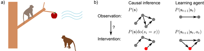
Figure 1: a) A causal relationship exists between the state of the branch and the state of the apple: if the branch is shaken, the apple can fall. By definition, it does not matter what intervenes on the branch to make it fall. This permits learning the causal relationship from a diverse range of sources: self action, another's action, or some other perturbation. b) Causal inference assumes an observational distribution, and asks when and how can we learn about what happens when intervening on the environment. Here, we argue the analogous setting in learning agents is to assume access to an observational distribution, and to study when and how this can be transferred to learn policies over action-conditioned distributions.
<details>
<summary>Image 1 Details</summary>
### Visual Description
\n
## Diagram: Causal Inference and Learning Agent
### Overview
The image presents a two-part diagram. Part (a) depicts a scenario with a monkey attempting to reach an apple suspended by a string. Part (b) illustrates the concepts of causal inference and a learning agent using graphical models. The diagram aims to visually connect a real-world problem (monkey reaching for an apple) with abstract concepts in machine learning and causal reasoning.
### Components/Axes
**Part (a):**
* **Elements:** A brown tree trunk, a branch, two monkeys (one on the branch, one on the ground), a string, an apple, wavy lines representing wind or movement.
* **Spatial Arrangement:** The monkey on the branch is reaching for the apple. The monkey on the ground is looking up. The apple is suspended by a string.
**Part (b):**
* **Sections:** Divided into two columns: "Causal Inference" and "Learning Agent". Each column has two rows: "Observation" and "Intervention".
* **Graphical Models:** Each section contains a graphical model represented by nodes (grey circles) and edges (lines connecting the nodes). One node in the "Intervention" section of the "Causal Inference" column is colored red.
* **Labels:**
* "Causal inference"
* "Learning agent"
* "Observation:"
* "Intervention:"
* "P(s)"
* "P(s | do(s₁ = x))"
* "P(sₜ₊₁ | sₜ)"
* "P(sₜ₊₁ | sₜ, aₜ)"
* A question mark ("?") between "Observation" and "Intervention" in the "Causal Inference" column.
### Detailed Analysis or Content Details
**Part (a):**
This section is a visual representation of a problem. There are no numerical values or specific data points. It depicts a monkey attempting to obtain an apple, potentially influenced by external factors like wind.
**Part (b):**
**Causal Inference Column:**
* **Observation:** The top graph shows a network of interconnected nodes (grey circles). The connections represent relationships between variables. The label "P(s)" is above this graph, likely representing the probability distribution of a state 's'.
* **Intervention:** The bottom graph shows a similar network, but with one node colored red. The label "P(s | do(s₁ = x))" is above this graph, indicating a probability distribution conditioned on an intervention where variable s₁ is set to x. The red node likely represents the variable being intervened upon.
**Learning Agent Column:**
* **Observation:** The top graph shows two nodes connected by a double-headed arrow. The label "P(sₜ₊₁ | sₜ)" is above this graph, representing the probability of the next state (sₜ₊₁) given the current state (sₜ).
* **Intervention:** The bottom graph shows three nodes connected in a triangular fashion. The label "P(sₜ₊₁ | sₜ, aₜ)" is above this graph, representing the probability of the next state (sₜ₊₁) given the current state (sₜ) and an action (aₜ).
### Key Observations
* The "Causal Inference" section uses graphical models to represent the concepts of observation and intervention. The red node in the "Intervention" graph highlights the variable being manipulated.
* The "Learning Agent" section uses graphical models to represent the transition probabilities in a Markov Decision Process (MDP). The inclusion of 'aₜ' (action) in the second graph indicates that the agent's actions influence the state transitions.
* The question mark in the "Causal Inference" section suggests a query or unknown relationship between observation and intervention.
* The diagram visually connects the real-world scenario in part (a) with the abstract concepts in part (b). The monkey's attempt to reach the apple can be seen as an intervention in a causal system.
### Interpretation
The diagram illustrates the relationship between causal inference and reinforcement learning. The monkey-apple scenario serves as an intuitive example of a problem that can be modeled using causal graphs and solved by a learning agent.
The "Causal Inference" section demonstrates how to reason about the effects of interventions in a system. By manipulating a variable (the red node), we can observe how it affects other variables.
The "Learning Agent" section shows how an agent can learn to make optimal decisions in an environment. The agent learns a policy that maps states to actions, maximizing its reward.
The diagram suggests that causal inference can be used to improve the performance of learning agents. By understanding the causal relationships in an environment, an agent can make more informed decisions and achieve better outcomes. The question mark highlights the challenge of identifying these causal relationships. The diagram is a conceptual illustration rather than a presentation of specific data. It aims to convey the underlying principles of causal reasoning and reinforcement learning.
</details>
at intervention-centric causal learning? By transferring from an observational setting to a setting where the agent is able to act on the environment, the agent exploits the fact that the observational and action phases share a common causal structure. This can be thought of as analogous to the typical problem in causal inference: how to transfer information from an observational distribution to candidate interventional ones (Figure 1b). While Problem 1 has been studied (Nair et al., 2019; Thomas et al., 2017; Sawada et al., 2018), to our knowledge Problem 2 has seen less attention. Yet arguably solutions to both are needed for a flexible learner that can fully exploit what it learns from observation and action.
We use a meta-reinforcement learning approach. The aim is that the agent learns for itself both what patterns of covariation indicate transferable relationships within the environment, and which of its actions may be able to exploit these relationships. In this way the agent performs causal learning in a flexible manner, without explicitly casting its environment into causal factors, and without having explicit labels that indicate when data is being drawn from different interventional distributions.
## 2 A MOTIVATING EXAMPLE
We start with a simple example. Consider a state space that factors into three variables: s t = ( s 1 t , s 2 t , s 3 t ) . Then suppose the environment has one of the two dynamic causal structures, where the differences between Model A and B is highlighted in bold :
- Model A (chain):
$$s _ { t } ^ { 1 } & = y _ { t } ^ { 1 } \\ s _ { t } ^ { 2 } & = y _ { t } ^ { 2 } + ( 1 - y _ { t } ^ { 2 } ) ( s _ { t - 1 } ^ { 1 } ) \\ s _ { t } ^ { 3 } & = y _ { t } ^ { 3 } + ( 1 - y _ { t } ^ { 3 } ) ( s _ { t - 1 } ^ { 2 } ) ,$$
<!-- formula-not-decoded -->
where y i t ∼ Bn ( p i ) denote Bernoulli random variables with probability of activation p i .
- And Model B (delayed fork):
<!-- formula-not-decoded -->
<!-- formula-not-decoded -->
Importantly, it is possible with certain parameter choices that, even though the models have a different causal structure, if all an agent observes is s t , it could not distinguish between Model A and Model B. It would have to interact with the system to tell the two apart. Consider then the task of learning which is the true causal structure. We will explore this problem using the meta-reinforcement learning approach of Wang et al. (2016), i.e. the same approach taken in Dasgupta et al. (2019) for causal inference through meta-RL, though they test their approach on static causal environments.
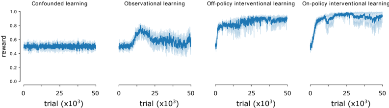
Figure 2: Average reward for meta-RL agent in simple causal inference environments. Curves show mean plus/minus standard error over n = 10 runs.
<details>
<summary>Image 2 Details</summary>
### Visual Description
## Line Chart: Learning Reward vs. Trial Number
### Overview
The image presents four line charts, each representing a different learning method: Confounded learning, Observational learning, Off-policy Interventional learning, and On-policy Interventional learning. Each chart plots the 'reward' on the y-axis against the 'trial' number (in thousands) on the x-axis. The charts visually compare the learning progress of each method over a series of trials.
### Components/Axes
* **X-axis Label:** "trial (x10³)" - Represents the number of trials, scaled in thousands. The scale ranges from 0 to 50 (representing 0 to 50,000 trials).
* **Y-axis Label:** "reward" - Represents the reward value. The scale ranges from 0.0 to 1.0.
* **Chart Titles:** Each chart has a title indicating the learning method: "Confounded learning", "Observational learning", "Off-policy interventional learning", "On-policy interventional learning".
* **Data Series:** Each chart contains a single blue line representing the reward over trials. The lines are accompanied by a shaded area representing the variance or standard deviation around the mean reward.
### Detailed Analysis
**1. Confounded Learning:**
* **Trend:** The line remains relatively flat throughout the trials, with minor fluctuations.
* **Data Points (approximate):**
* Trial 0: Reward ≈ 0.45
* Trial 25,000: Reward ≈ 0.48
* Trial 50,000: Reward ≈ 0.46
* The reward fluctuates between approximately 0.4 and 0.55.
**2. Observational Learning:**
* **Trend:** The line starts at a similar level as confounded learning, but exhibits a significant upward trend starting around trial 10,000, plateauing around trial 40,000.
* **Data Points (approximate):**
* Trial 0: Reward ≈ 0.45
* Trial 10,000: Reward ≈ 0.60 (start of upward trend)
* Trial 25,000: Reward ≈ 0.85
* Trial 50,000: Reward ≈ 0.90
* The reward increases from approximately 0.4 to 0.9.
**3. Off-policy Interventional Learning:**
* **Trend:** Similar to observational learning, the line shows an upward trend, but it begins earlier and reaches a higher plateau.
* **Data Points (approximate):**
* Trial 0: Reward ≈ 0.45
* Trial 5,000: Reward ≈ 0.65 (start of upward trend)
* Trial 25,000: Reward ≈ 0.95
* Trial 50,000: Reward ≈ 0.98
* The reward increases from approximately 0.4 to 0.98.
**4. On-policy Interventional Learning:**
* **Trend:** The line exhibits a rapid initial increase, followed by a plateau. The initial increase is steeper than the other methods.
* **Data Points (approximate):**
* Trial 0: Reward ≈ 0.45
* Trial 5,000: Reward ≈ 0.75 (start of upward trend)
* Trial 15,000: Reward ≈ 0.95
* Trial 50,000: Reward ≈ 0.98
* The reward increases from approximately 0.4 to 0.98.
### Key Observations
* Confounded learning shows minimal improvement over trials.
* Observational, Off-policy, and On-policy learning all demonstrate significant improvement in reward over trials.
* On-policy learning exhibits the fastest initial learning rate.
* Off-policy and On-policy learning achieve the highest final reward values.
* The shaded areas indicate variability in the reward, which appears consistent across all learning methods.
### Interpretation
The data suggests that interventional learning methods (Off-policy and On-policy) are significantly more effective than observational or confounded learning in maximizing reward. The faster learning rate of On-policy learning indicates that it may be more efficient in converging to an optimal policy. The minimal improvement in confounded learning suggests that it is unable to effectively learn from the environment due to underlying confounding factors. The variance in reward, represented by the shaded areas, indicates that the learning process is stochastic and subject to fluctuations. The charts provide a comparative analysis of different learning approaches, highlighting the benefits of interventional learning in achieving higher rewards. The differences in learning curves suggest that the methods have different exploration-exploitation trade-offs and sensitivities to the environment.
</details>
## 2.1 META-LEARNING AGENT ARCHITECTURE
The meta-reinforcement learning approach works as follows. A task, or trial, is sampled from some distribution D . Here, this just means one of Model A or B is chosen with probability p A = 0 . 5 . Within the trial, states are generated according to the appropriate model, for N steps. An LSTM network (Hochreiter and Schmidhuber, 1997) (with 48 hidden units) was used. At each time step the LSTM receives the vector ( s t , a t -1 , r t -1 ) as input, where s t is the observation, a t -1 is the previous action (as a one-hot vector) and r t -1 the reward (as a single real-value). The outputs are a linear function of the LSTM's state. A set of logits are output (with dimensionality equal to the number of available actions), plus a scalar baseline. A softmax is applied to the logits, and then sampled to give a selected action. Learning was by the asynchronous advantage actor-critic (A3C) (Mnih et al., 2016) algorithm. In this framework, the loss function consists of three terms: the policy gradient, the baseline cost and an entropy cost. The baseline cost was weighted by 0.05 relative to the policy gradient cost. Optimization was done by ADAM optimization with learning rate 10 -3 , β 1 = 0 . 9 , β 2 = 0 . 999 , = 10 -7 . What follows was implemented in TensorFlow.
## 2.2 TASK DETAILS
The agent is presented with N = 10 observations from a sequence s t generated according to either Model A or Model B. The agent is rewarded at the end of the trial for correctly identifying the true model. That is, the action space is A = { A,B } . If a N is the correct model, then reward r N = 1 is given. Otherwise r N = 0 . At all other times in the trial, the reward is zero. We compare performance of this meta-RL approach in four different settings, each providing different amount of information to the agent, and allowing different levels of interaction with the environment. The specific values for these models are provided in the supplementary material.
1. Confounded - the agent only observes s t , thus has insufficient information to solve the problem.
2. Observational - there are now perturbations of the environment, changing the distribution over s t , but these perturbations are unobserved. More specifically, z i t ∼ Bn ( p int i ) are 'intervention indicator' variables sampled at each time step. If z i t = 1 then y i t = 1 , otherwise it follows the same dynamics as before. For some cases, this may allow the agent to identify the true causal structure.
3. Off-policy interventional - the agent now observes the perturbations z t , concatenated onto s t . Now the correct structure is identifiable, provided the agent can learn which of z 2 and z 3 are associated with each node s 2 and s 3 .
4. On-policy interventional - now the action space of the agent is the perturbation-space z . In this case, the action space for the agent can be considered as interventions on the environment. Here the agent additionally observes a go cue, at the end of the trial, to indicate it should provide its response as to which is the correct underlying model.
## 2.3 RESULTS AND DISCUSSION
Though this is a very simple example, it captures different forms of causal learning. In the purely observational setting, in this case, no causal learning is possible. In the observational with perturbations setting, causal learning may be possible, and is akin to something like emulative learning with 'ghost conditions' in cognitive science (e.g. the wind blowing the branch thought experiment above) (Hopper, 2010). In the off-policy interventional setting, causal learning may again be possible, and may be aided by learning to exploit the additional observed cues that a variable is being perturbed from its default dynamics, z . Finally, in the on-policy interventional setting, the agent can learn the causal model directly through its own interventions - agent-centric causal learning possible through any reinforcement learning algorithm. The results using the meta-RL algorithm show both the onand off-policy interventional settings are indeed solvable after a few thousand trials (Figure 2).
This setup allowed us to explore causal learning under two significant Assumptions:
1. The causal relationships are expressed more or less directly between the observed variables, the causal structure is not latent. 1 Further, the variables indicating whether and which variable was being perturbed were also directly observed, at least in the relevant setting.
2. The action space is given as direct manipulations of the underlying causal variables.
These assumptions relate to Problems 1 and 2 described in the introduction. Thus, to extend current approaches, we consider ways in which these assumptions can be dropped.
## 3 DEALING WITH LATENT CAUSAL STRUCTURE
We can first study settings that relax Assumption 1. In fact this is very close to the problem tackled by Nair et al. (2019), except in their case the focus is on planning to reach a goal state. And in their case the actions can be taken as direct manipulations of the underlying causal variables, an assumption we will drop in the next section.
## 3.1 TASK DETAILS
To extend our simple example to this case, we consider an 8x8x3 observation space, denoted o t . Three pixels in this space correspond to the state of s 1 t , s 2 t , s 3 t , obeying the same dynamics as in the previous section. When active, the corresponding pixel is colored white, otherwise it is black. Then, to mix the state of these variables in the observations, a Gaussian blur is applied to the image. In the relevant conditions, the additional indicator variables z t are added in the same locations as s i , but are added only to the red channel. Further, the observed image at each frame t is a 50-50 mix of the previous frame o t -1 and the current one (the Gaussian blurred pixels corresponding to the state of the system at frame t ). This introduces some temporal blurring in the observed dynamics also (Figure 3a). Now the relationship between the variables y i and the observed images is less obvious. As before, reward r N = 1 , is given for correctly identifying the underlying model, and r N = 0 otherwise. The observed image o t is fed to the learning agent, instead of the underlying state s t
## 3.2 RESULTS
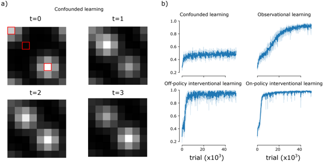
The meta-RL agent's architecture is modified to add a fully connected layer of size 64, with inputs over the flattened image, before being fed to the LSTM. With this change, the learner is able to quickly learn the correct model. In the interventional conditions, it can learn how to figure out the correct model after only a few thousand trials. The observational setting takes closer to fifty thousand trials to reach the same performance (Figure 3b). Nonetheless, the agent is able to learn the latent causal structure underlying the observations in all but the confounded case.
1 Technically, the delay introduces some degree of unobservedness.
Figure 3: Environment with latent causal structure. a) Four frames from the confounded environment condition. Three, blurred, flashing pixels indicate the state of the variables y t , obeying either chain or delayed fork dynamics between them. For illustration, these are highlighted in red, though this information isn't provided to the agent. The activated pixels decay over time. The other settings are similar, with additional flags to represent the state of z t , where relevant. b) Curves show mean reward plus/minus standard error over n = 10 runs.
<details>
<summary>Image 3 Details</summary>
### Visual Description
## Image Analysis: Learning Dynamics Visualization
### Overview
The image presents a visualization of learning dynamics under different learning paradigms. Part (a) shows a series of heatmaps representing the learned value function over time (t=0 to t=3) for "Confounded learning". A red square highlights a region of interest in the initial heatmap. Part (b) displays learning curves for four different learning methods: Confounded learning, Observational learning, Off-policy Interventional learning, and On-policy Interventional learning. The learning curves plot performance (y-axis, ranging from 0 to 1.0) against the number of trials (x-axis, in units of 10^3).
### Components/Axes
**Part (a): Confounded Learning Heatmaps**
* **Title:** "Confounded learning" (top-center)
* **Time Steps:** t=0, t=1, t=2, t=3 (labeled above each heatmap)
* **Heatmap Intensity:** Represents the value function, with lighter shades indicating higher values and darker shades indicating lower values.
* **Red Square:** Located in the top-left heatmap (t=0), indicating a specific region of interest.
**Part (b): Learning Curves**
* **Title:** Four subplots, each with a learning method title: "Confounded learning", "Observational learning", "Off-policy Interventional learning", "On-policy Interventional learning".
* **X-axis:** "trial (x10³)" ranging from approximately 0 to 45,000.
* **Y-axis:** A scale from 0.0 to 1.0, representing performance.
* **Data Series:** Each subplot contains a single blue line representing the learning curve, with a shaded area indicating the standard deviation.
### Detailed Analysis or Content Details
**Part (a): Confounded Learning Heatmaps**
* **t=0:** The heatmap shows a bright spot in the center and a red square in the top-left corner. The intensity is highest in the center.
* **t=1:** The bright spot has spread and become less focused. The intensity is still highest in the center, but the red square region has diminished in intensity.
* **t=2:** The bright spot continues to spread, becoming more diffuse. The intensity is still centered.
* **t=3:** The bright spot is now quite diffuse, with a broad area of moderate intensity. The intensity is still centered.
**Part (b): Learning Curves**
* **Confounded Learning:** The learning curve starts at approximately 0.2 and gradually increases to around 0.6, with significant fluctuations. It plateaus around 0.6.
* **Observational Learning:** The learning curve starts at approximately 0.2 and rapidly increases to around 0.95, with minimal fluctuations. It plateaus around 0.95.
* **Off-policy Interventional Learning:** The learning curve starts at approximately 0.2 and rapidly increases to around 0.85, with some fluctuations. It plateaus around 0.85.
* **On-policy Interventional Learning:** The learning curve starts at approximately 0.2 and rapidly increases to around 0.9, with minimal fluctuations. It plateaus around 0.9.
### Key Observations
* The "Confounded learning" heatmap shows how the learned value function spreads over time, potentially indicating a lack of precise localization.
* The "Confounded learning" learning curve exhibits slow and unstable learning, reaching a relatively low performance level.
* "Observational learning" and "On-policy Interventional learning" demonstrate fast and stable learning, achieving high performance levels.
* "Off-policy Interventional learning" shows fast learning, but plateaus at a slightly lower performance level than "Observational learning" and "On-policy Interventional learning".
### Interpretation
The image demonstrates the impact of different learning paradigms on learning dynamics and performance. The "Confounded learning" approach appears to suffer from a lack of precision in the learned value function (as seen in the spreading heatmap) and slow, unstable learning (as seen in the learning curve). This suggests that confounding factors hinder the agent's ability to accurately estimate the value of different states.
In contrast, "Observational learning" and the interventional learning methods exhibit faster and more stable learning, indicating that they are more effective at overcoming the challenges posed by confounding factors. The slight difference in performance between "Off-policy" and "On-policy" interventional learning might be due to the inherent biases associated with off-policy learning.
The red square in the initial heatmap (t=0) likely represents the initial focus of the learning agent. The subsequent spreading of the bright spot suggests that the agent is struggling to maintain its focus and is instead generalizing its value estimates across a broader range of states. This generalization could be a consequence of the confounding factors, which prevent the agent from accurately distinguishing between different states.
</details>
## 4 CAUSAL LEARNING IN AGENT-CENTRIC ACTION SPACES
We now focus on the setting that relaxes Assumption 2. That is, the action space is now ego-centric, and cannot be interpreted as a direct manipulation of the relevant causal variables underlying the model dynamics. To test causal learning in this setting, we use a simple grid-world environment.
## 4.1 TASK DETAILS
The task is an 'escape room' task. The environment consists of a 5x5 grid-world. On three edges of the grid are buttons. When anything overlaps with the pixel adjacent to the button, it is pushed. In a given trial of N steps, only one of the buttons (chosen uniformly at random) will activate/open the door on the fourth wall. This door will stay open for T time steps.
There are two phases to this environment. In the first observational phase, for N O steps, a white object bounces randomly between the three buttons, occasionally activating the door. The agent's actions are ineffective. In the second phase, the action phase, a green cue in the upper left corner indicates that the agent's actions now effect the environment - they move a separate (gray) object around the grid-world (Figure 4a). While the bouncing object can move one pixel in the cardinal directions, or one pixel diagonally, the agent can only move one pixel in the four cardinal directions. This phase lasts N A steps. The agent is rewarded if it moves to the pixel immediately adjacent to the open door. A reward of R d is administered.
We test the case that N A is too small for a valid policy to be the agent, in the action phase, tries each button sequentially to see which one opens the door - to solve the task it has to pay attention to the observation phase state transitions. Here N O = 20 , N A = 10 , the door is open for T = 5 time steps, and the reward is R d = 10 .
## 4.2 RESULTS
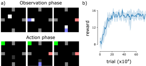
The same network architecture and algorithm as the previous section is used. With this, the meta-RL agent is able to learn to perform this causal learning task after about two hundred thousand trials (Figure 4b). The agent start location is randomly chosen, at the start of each action phase. It then successfully moves to the correct button, and then to the door for reward on a high proportion of trials. Thus this setup is able to successfully utilize information from the observation phase for use in the action phase. In doing so the agent is not mimicking the movement of the white box; it is
Figure 4: The escape-room environment. a) Task involves observation phase, in which the white box bounces randomly between the three buttons (all but the right). When the box is adjacent to the randomly chosen button that opens the door for that trial, it turns red. In the action phase, the agent moves the gray box around. It has to learn from the previous phase which button to go for to open the door and move to it in time to get reward. Some frames are skipped for simplicity in this illustration. b) Curves show mean reward plus/minus standard error over n = 5 runs.
<details>
<summary>Image 4 Details</summary>
### Visual Description
## Diagram & Chart: Reinforcement Learning Environment & Reward Curve
### Overview
The image presents a reinforcement learning environment visualized as a grid world, alongside a chart showing the reward received over training trials. The grid world is shown in two phases: Observation and Action. The chart displays the average reward as a function of the trial number.
### Components/Axes
**Diagram (a):**
* **Title:** "Observation phase" and "Action phase"
* **Grid:** A 6x6 grid with cells colored black, gray, white, blue, green, and red.
* **Agent Representation:** White (Observation), Blue (Observation), Green (Action), Red (Action).
* **Grid Cell States:** Black (empty), Gray (obstacle).
**Chart (b):**
* **Title:** None explicitly stated, but implied to be "Reward vs. Trial"
* **X-axis:** "trial (x10⁴)" - ranging from approximately 0 to 60 (in units of 10,000 trials).
* **Y-axis:** "reward" - ranging from approximately 6 to 16.
* **Data Series:** A single blue line representing the average reward, with a shaded region indicating the standard deviation or confidence interval.
### Detailed Analysis or Content Details
**Diagram (a): Observation Phase (Top Row)**
The observation phase shows the agent (represented by white and blue squares) navigating a grid with obstacles (gray squares). The sequence of states is as follows:
1. White square in the top-left corner.
2. Blue square moves one cell to the right.
3. Blue square moves one cell down.
4. Blue square moves one cell down, and a red square appears in the bottom-right corner.
**Diagram (a): Action Phase (Bottom Row)**
The action phase shows the agent (represented by green and red squares) taking actions in the same grid. The sequence of states is as follows:
1. Green square in the top-left corner.
2. Green square remains in the same position.
3. Red square moves one cell up.
4. Red square moves one cell up, and a blue square appears in the bottom-left corner.
**Chart (b): Reward Curve**
The reward curve shows a clear learning trend.
* **Initial Phase (0-20 x10⁴ trials):** The reward increases rapidly from approximately 7 to 14.
* **Plateau Phase (20-40 x10⁴ trials):** The reward plateaus around 15, with fluctuations.
* **Decline Phase (40-60 x10⁴ trials):** The reward decreases from approximately 15 to 12, with fluctuations.
Approximate data points (reading from the chart):
* Trial 0 x10⁴: Reward ≈ 7
* Trial 10 x10⁴: Reward ≈ 12
* Trial 20 x10⁴: Reward ≈ 14
* Trial 30 x10⁴: Reward ≈ 15
* Trial 40 x10⁴: Reward ≈ 15
* Trial 50 x10⁴: Reward ≈ 13
* Trial 60 x10⁴: Reward ≈ 12
### Key Observations
* The agent appears to observe its environment and then take actions based on that observation.
* The reward curve indicates successful learning initially, followed by a period of stabilization and then a slight decline in performance.
* The shaded region in the chart suggests variability in the reward obtained across different trials.
### Interpretation
The image demonstrates a reinforcement learning setup where an agent learns to navigate a grid world. The observation phase allows the agent to perceive its environment, while the action phase allows it to interact with it. The reward curve shows that the agent initially learns to maximize its reward, but its performance may degrade over time, potentially due to overfitting or changes in the environment. The decline in reward after 40 x10⁴ trials could indicate the need for further exploration or adjustments to the learning algorithm. The grid world setup is a simplified representation of a more complex environment, but it provides a useful framework for understanding the principles of reinforcement learning. The color coding of the grid cells (white, blue, green, red, gray, black) likely represents different states or features of the environment, such as the agent's position, obstacles, or goal locations.
</details>
not performing imitation learning. This transfer from observation to action is a key indicator of intervention-centric causal learning.
## 5 DISCUSSION
In essence here we proposed to take a step back from a causal formalism such as Pearl's (Pearl, 2000) and ask how behaviors that constitute interventions and observational learning as studied in cognitive science can be recapitulated in a learning agent. Interventions in this sense are a more vague notion than in a statistical causal model, which takes the exact mechanism of the intervention as given. But the human and animal cognitive science literature has studied interventions in many settings and stages of development. So we can better understand what behaviors constitute sophisticated causal reasoning by turning to these studies.
## 5.1 INSPIRATION FROM COGNITIVE SCIENCE
What notion of causality do we and other animals possess? Philosopher James Woodward (Woodward, 2010) argues that a notion of interventions is unique to humans. Other animals have either an egocentric notion of causality - they are only capable of learning causal relationships as they are revealed by and apply to the agent; or an agent-centric notion of causality, in which learning the structure of the world can also be achieved through reproducing another agent's actions.
Operant conditioning is of course ubiquitous among animals, and thus so is agent-centric causal learning. This type of learning can be quite sophisticated: tool-using animals demonstrate a nuanced understanding of the consequences of their actions (Schloegl and Fischer, 2017), and model-based reinforcement learning involves learning a causal model of the environment (Gershman, 2017). Yet such learning does not require a notion of an environment with structure independent of the agent's actions, and thus no sense in which actions are interventions on that environment.
Social learning amongst animals too can be quite complicated. In imitative learning, the actions of another agent are copied to achieve some goal. In emulative learning, an observed action is not necessarily reproduced, but an action is taken to reproduce a desired, observed outcome (Hopper, 2010). However, the causal learning that occurs in these cases may not be perfect: animals may not show an understanding of the relevant parts of another agent's actions to copy, leading to overimitation - performing a sub-optimal action simply because the demonstrator did, while control animals that only try the task for themselves learn the optimal action more quickly (Hopper, 2010). For these reasons, social learning is also not indicative of a full causal understanding of the environment either.
These can be contrasted with an intervention-centric notion of causality. The hallmarks of which are the ability to appropriately imitate and emulate others' actions to produce a desired goal, to not over-imitate, to not misuse tools or select the wrong tool for the job, to produce novel interventions
that are suggested by relationships learned from observation, and to learn and integrate relationships from a diverse range of sources (not just from others). Though animals such as primates and corvids, and children, can perform some of these (Tennie et al., 2010; Meltzoff et al., 2012; Bonawitz et al., 2010; Hopper et al., 2008; Schloegl and Fischer, 2017; Völter et al., 2016; Bonawitz et al., 2010; Taylor et al., 2015; 2014; Jelbert et al., 2014; Taylor et al., 2007), adult humans can most robustly perform each of these things.
## 5.2 RELATED WORK AND OUTLOOK
Here we focused on a notion of causal learning relatively unaddressed in the learning agent literature. We provided a simple environment that gets at this issue, and one simple meta-RL algorithm that can solve it. However we do not propose any algorithmic innovations: there may be better approaches, and these may be closely related to those already in use. It's thus useful to highlight related work.
The environment presented here requires the agent to take advantage of data drawn from an observational setting, in which the actions of the agent are ineffective. This is related to learning problems where the action labels generating the observed state sequences are not provided. This setting has been explored recently in imitation learning settings, known as imitation learning from observation (ILO) (Torabi et al., 2019b;a; Ho and Ermon, 2016; Zołna et al., 2019; Zolna et al., 2019; Torabi et al., 2018; Li et al., 2018; Liu et al., 2018; Wu et al., 2018; Edwards et al., 2018). But these methods do not solve the problem by themselves - they just imitate. Imitating for the sake of it, over-imitation, is a sign of a lack of causal understanding. Recent work combining imitation learning and reinforcement learning, or learning from imperfect demonstrations (Gao et al., 2018), address this to some extent (Zołna et al., 2019). RILO does so in a setting where action labels are not provided (Zołna et al., 2019). However such approaches, when no reward signal is available, will default to imitation learning. This may be a practical learning approach in the presence of an expert, but it does not get at causal learning. Though some version of these works may prove promising in the task domain we have tested here.
Alternatively we can approach the problem by eschewing imitation learning, and viewing the setting presented here as doing a form of off-policy reinforcement learning where action labels are not provided (similar to Borsa et al. (2017)). Some of the approaches used in ILO may prove still useful. For instance, models based on inverse dynamics models could take the observational data (Christiano et al., 2016; Pathak et al., 2017), use the inverse model to infer what action the agent could have taken, and then run an RL algorithm using the inferred actions. A sort of vicarious learning, evocative of agency theories of causation (Woodward, 2010). A comparison between this approach and that taken here is future work.
Acaveat is that here we have just focused on the idea of transferring what is learnt from observation to an action phase. But, in addition to this transferability, a key notion in intervention-based learning is that interventions are specific - they only act on a particular object. An algorithm's ability to parse the environment into a discrete set of objects, and to learn how these could be manipulated individually, was not tested. This problem relates to recent work on learning environment affordances and controllable factors (Thomas et al., 2017; Sawada et al., 2018). Methods like Recurrent Independent Mechanisms (Goyal et al., 2019) have proposed learning separable components of an environment with their own autonomous dynamics, which may relate to causal factors in the environment, and thus may prove useful in this regard.
Closely related to ideas of transferring from observational to action settings is work in the causal inference literature that learns causal models from unknown or uncertain interventions. In invariant causal prediction (Peters et al., 2016; Arjovsky et al., 2019), for instance, robustness to changes in environment are used as a cue for causal relations. These ideas has been explored in a meta-learning setting too (Bengio et al., 2019). Emerging ideas of the importance of invariance needs to be integrated with this intervention-centric notion used here (Arjovsky et al., 2019; Schölkopf, 2019). Finally, and perhaps most related to the work here is work on meta-learning causal learning algorithms (Dasgupta et al., 2019). This work differs from that here in that the environment is low-dimensional, almost fully observed, not dynamic, and the actions are taken as manipulations of the state variables in the causal graph. Thus there is a lot of progress in all of these related areas. A more explicit testing of these learning agents' causal learning abilities in the settings such as those tested here may prove useful in providing AI with a more human-like notion of causality.
## ACKNOWLEDGEMENTS
For many useful discussions, the author thanks Anna Leshinskaya and Anirudh Goyal.
## REFERENCES
- Martin Arjovsky, Leon Bottou, Ishaan Gulrajani, and David Lopez-Paz. Invariant Risk Minimization. ArXiv e-prints , pages 1-30, 2019.
- Elias Bareinboim and Judea Pearl. Causal inference and the data-fusion problem. Proceedings of the National Academy of Sciences , 113(27):7345-7352, 2016. ISSN 0027-8424. doi: 10.1073/pnas.1510507113. URL http://www.pnas.org/lookup/doi/10.1073/pnas.1510507113 .
- Elias Bareinboim, Andrew Forney, and Judea Pearl. Bandits with Unobserved Confounders: A Causal Approach. Advances in Neural Information Processing Systems , pages 1-9, 2015. ISSN 10495258.
- Yoshua Bengio, Tristan Deleu, Nasim Rahaman, Nan Rosemary Ke, Olexa Bilaniuk, Anirudh Goyal, and Christopher Pal. A meta-transfer objective for learning to disentangle causal mechanisms. ArXiv e-prints , pages 1-26, 2019.
- Elizabeth Baraff Bonawitz, Darlene Ferranti, Rebecca Saxe, Alison Gopnik, Andrew Meltzoff, James Woodward, and Laura E. Schulz. Just do it? Investigating the gap between prediction and action in toddlers' causal inferences. Cognition , 115(1):104-117, 2010. doi: 10.1016/j.cognition.2009.12.001.Just.
- Diana Borsa, Olivier Pietquin, Rémi Munos, and Bilal Piot. Observational Learning by Reinforcement Learning. ArXiv e-prints , 2017.
- Paul Christiano, Zain Shah, Igor Mordatch, Jonas Schneider, Trevor Blackwell, Joshua Tobin, Pieter Abbeel, and Wojciech Zaremba. Learning Deep Inverse Dynamics Model. ArXiv e-prints , 2016.
- Ishita Dasgupta, Jane Wang, Silvia Chiappa, Jovana Mitrovic, Pedro Ortega, David Raposo, Edward Hughes, Peter Battaglia, Matthew Botvinick, and Zeb Kurth-nelson. Causal Reasoning from Meta-reinforcement learning. ArXiv e-prints , 2019. URL https://openreview.net/forum?id=H1ltQ3R9KQ .
- Ashley D. Edwards, Himanshu Sahni, Yannick Schroecker, and Charles L. Isbell. Imitating Latent Policies from Observation. ArXiv e-prints , 2018. URL http://arxiv.org/abs/1805.07914 .
- Yang Gao, Huazhe, Xu, Ji Lin, Fisher Yu, Sergey Levine, and Trevor Darrell. Reinforcement Learning from Imperfect Demonstrations. ArXiv e-prints , 2018. ISSN 0004-6361. doi: 10.1051/0004-6361/201527329. URL http://arxiv.org/abs/1802.05313 .
- Samuel J Gershman. Reinforcement learning and causal models. In Oxford Handbook of Causal Reasoning , pages 1-32. Oxford university press, 2017.
- Alison Gopnik and Laura Schulz. Causal learning: Psychology, philosophy, and computation . Oxford University Press, 2007.
- Anirudh Goyal, Alex Lamb, Jordan Hoffmann, Shagun Sodhani, Sergey Levine, Yoshua Bengio, and Bernhard Schölkopf. Recurrent Independent Mechanisms. ArXiv e-prints , pages 1-33, 2019. URL http://arxiv. org/abs/1909.10893 .
- Jonathan Ho and Stefano Ermon. Generative Adversarial Imitation Learning. ArXiv e-prints , 2016.
- Sepp Hochreiter and Jurgen Schmidhuber. Long short-term memory. Neural Computation , 9(8):1-32, 1997. ISSN 0899-7667. doi: 10.1162/neco.1997.9.8.1735.
- Lydia M. Hopper. 'Ghost' experiments and the dissection of social learning in humans and animals. Biological Reviews , 85(4):685-701, 2010. ISSN 14647931. doi: 10.1111/j.1469-185X.2010.00120.x.
- Lydia M Hopper, Susan P Lambeth, Steven J Schapiro, and Andrew Whiten. Observational learning in chimpanzees and children studied through ' ghost ' conditions. Proceedings of the Royal Society B , 275 (January):835-840, 2008. doi: 10.1098/rspb.2007.1542.
- Sarah A Jelbert, Alex H Taylor, Lucy G Cheke, Nicola S Clayton, and Russell D Gray. Using the Aesop' s Fable Paradigm to Investigate Causal Understanding of Water Displacement by New Caledonian Crows. PLoS ONE , 9(3), 2014. doi: 10.1371/journal.pone.0092895.
- Guohao Li, Matthias Mueller, Vincent Casser, Neil Smith, Dominik L. Michels, and Bernard Ghanem. Teaching UAVs to Race With Observational Imitation Learning. ArXiv e-prints , 2018. URL http://arxiv.org/ abs/1803.01129 .
- Yuxuan Liu, Abhishek Gupta, Pieter Abbeel, Sergey Levine, and Computer Science. Imitation from Observation : Learning to Imitate Behaviors from Raw Video via Context Translation. ArXiv e-prints , 2018.
- Andrew N Meltzoff, Anna Waismeyer, and Alison Gopnik. Learning about causes from people: observational causal learning in 24-month-old infants. Dev Psychol. , 48(5):1215-1228, 2012. doi: 10.1037/a0027440. Learning.
- Volodymyr Mnih, Adrià Puigdomènech Badia, Mehdi Mirza, Alex Graves, Timothy P. Lillicrap, Tim Harley, David Silver, Koray Kavukcuoglu, Timothy P. Lillicrap, and David Silver. Asynchronous methods for deep reinforcement learning. ArXiv e-prints , 48:1-28, 2016. ISSN 1938-7228. URL http://arxiv.org/ abs/1602.01783 .
- Suraj Nair, Yuke Zhu, Silvio Savarese, and Li Fei-Fei. Causal induction from visual observations for goal directed tasks. ArXiv e-prints , pages 1-13, 2019.
- Deepak Pathak, Pulkit Agrawal, Alexei A. Efros, and Trevor Darrell. Curiosity-driven Exploration by Selfsupervised Prediction. ArXiv e-prints , 2017. ISSN 1938-7228. doi: 10.1109/CVPRW.2017.70. URL http://arxiv.org/abs/1705.05363 .
- Judea Pearl. Causality: models, reasoning and inference . Cambridge Univ Press, 2000.
- J Peters, D Janzing, and B Schölkopf. Elements of Causal Inference: Foundations and Learning Algorithms . MIT Press, Cambridge, MA, USA, 2017.
- Jonas Peters, Peter Bühlmann, and Nicolai Meinshausen. Causal inference using invariant prediction: identification and confidence intervals. Journal of the Royal Statistical Society: Series B (Statistical Methodology) , pages 1-42, 2016. URL http://arxiv.org/abs/1501.01332 .
- Yoshihide Sawada, Luca Rigazio, Koji Morikawa, Masahiro Iwasaki, and Yoshua Bengio. Disentangling Controllable and Uncontrollable Factors by Interacting with the World. Advances in Neural Information Processing Systems , 2018.
- Christian Schloegl and Julia Fischer. Causal Reasoning in Non-Human Animals. In Oxford Handbook of Causal Reasoning , pages 1-33. Oxford University Press, 2017. ISBN 9780199399550. doi: 10.1093/oxfordhb/ 9780199399550.013.36.
- Bernhard Schölkopf. Causality for Machine Learning. ArXiv e-prints , pages 1-20, 2019.
- Richard Sutton and Andrew Barto. Reinforcement Learning: An Introduction . The MIT Press, 2017. ISBN 0262193981. doi: 10.1016/S1364-6613(99)01331-5. URL http://linkinghub.elsevier.com/ retrieve/pii/S1364661399013315 .
- Alex H Taylor, Gavin R Hunt, C Holzhaider, and Russell D Gray. Spontaneous Metatool Use by New Caledonian Crows. Current Biology , 17:1504-1507, 2007. doi: 10.1016/j.cub.2007.07.057.
- Alex H Taylor, Lucy G Cheke, Anna Waismeyer, Andrew N Meltzoff, Rachael Miller, Alison Gopnik, Nicola S Clayton, Russell D Gray, and Alex H Taylor. Of babies and birds : complex tool behaviours are not sufficient for the evolution of the ability to create a novel causal intervention. Proceedings of the Royal Society B , 281, 2014.
- Alex H Taylor, Lucy G Cheke, Anna Waismeyer, Andrew Meltzoff, Rachael Miller, Alison Gopnik, Nicola S Clayton, Russell D Gray, Clayton Ns, Gray Rd, and Alex H Taylor. No conclusive evidence that corvids can create novel causal interventions. Proceedings of the Royal Society B , 282:6-8, 2015. doi: 10.1098/rspb.2014. 2504.
- Claudio Tennie, Kathrin Greve, and Heinz Gretscher. Two-year-old children copy more reliably and more often than nonhuman great apes in multiple observational learning tasks. Primates , 51:337-351, 2010. doi: 10.1007/s10329-010-0208-4.
- Valentin Thomas, Jules Pondard, Emmanuel Bengio, Marc Sarfati, Philippe Beaudoin, Marie-Jean Meurs, Joelle Pineau, Doina Precup, and Yoshua Bengio. Independently Controllable Factors. ArXiv e-prints , pages 1-13, 2017. URL http://arxiv.org/abs/1708.01289 .
- M Tomasello and J Call. Primate Cognition . Primate Cognition. Oxford University Press, 1997. ISBN 9780195106244. URL https://books.google.ca/books?id=bSYdl2ExJrEC .
- Faraz Torabi, Garrett Warnell, and Peter Stone. Behavioral Cloning from Observation. IJCAI , 2018. URL http://arxiv.org/abs/1805.01954 .
- Faraz Torabi, Garrett Warnell, and Peter Stone. Generative Adversarial Imitation from Observation. ArXiv e-prints , 2019a.
- Faraz Torabi, Garrett Warnell, and Peter Stone. Recent Advances in Imitation Learning from Observation. Joint Conference on Artificial Intelligence , (August), 2019b.
- Christoph J Völter, Inés Sentís, and Josep Call. Great apes and children infer causal relations from patterns of variation and covariation. Cognition , 155:30-43, 2016. doi: 10.1016/j.cognition.2016.06.009.
- Jane X Wang, Zeb Kurth-Nelson, Dhruva Tirumala, Hubert Soyer, Joel Z Leibo, Remi Munos, Charles Blundell, Dharshan Kumaran, and Matt Botvinick. Learning to reinforcement learn. ArXiv e-prints , pages 1-17, 2016. URL http://arxiv.org/abs/1611.05763 .
- James Woodward. Making things happen: A theory of causal explanation . Oxford university press, 2003.
- James F. Woodward. Agency and Interventionist Theories. In The Oxford Handbook of Causation , number May 2017, pages 1-30. Oxford University Press, 2010. ISBN 9780191577246. doi: 10.1093/oxfordhb/ 9780199279739.003.0012.
- Jim Woodward. Causation with a Human Face, 2007.
- Yueh-Hua Wu, Nontawat Charoenphakdee, Han Bao, Voot Tangkaratt, and Masashi Sugiyama. Imitation Learning from Imperfect Demonstration. ArXiv e-prints , pages 1-25, 2018. URL https://www. basketball-reference.com/leagues/NBA{\_}stats.html .
- Junzhe Zhang and Elias Bareinboim. Markov Decision Processes with Unobserved Confounders: A Causal Approach. Technical Report R-23, Purdue AI Lab , 2016.
- Junzhe Zhang and Elias Bareinboim. Transfer learning in multi-armed bandits: A Causal approach. IJCAI International Joint Conference on Artificial Intelligence , pages 1340-1346, 2017. ISSN 10450823.
- Konrad Zolna, Scott Reed, Alexander Novikov, Sergio Gomez Colmenarej, David Budden, Serkan Cabi, Misha Denil, Nando de Freitas, and Ziyu Wang. Task-Relevant Adversarial Imitation Learning. Advances in neural information processing - Deep Reinforcement Learning Workshop , pages 1-16, 2019. URL http://arxiv.org/abs/1910.01077 .
- Konrad Zołna, Negar Rostamzadeh, Yoshua Bengio, Sungjin Ahn, and Pedro Pinheiro. Reinforced Imitation in Heterogeneous Action Space. ArXiv e-prints , pages 1-17, 2019.
## A PARAMETERS FOR ENVIRONMENTS
## A.1 SIMPLE ENVIRONMENT PARAMETERS
Trial lasts N = 20 steps. The probability of a given trial having the chain structure is 0.5. Spontaneous rates of activation for s i : p 1 = 0 . 1 , p 2 = 0 . 01 , p 3 = 0 . 01 . For the off-policy settings with the 'interventional' variables ( z i ), these are activated with probabilities p int 2 = 0 . 1 , p int 3 = 0 . 1 . Only the second and third variables are perturbed - a perturbation of the parent node s 1 t will not help discriminate between the two Models.
## A.2 VISUAL ENVIRONMENT PARAMETERS
The underlying dynamics have the same parameters as the basic environments.
## A.3 AGENT-CENTRIC ENVIRONMENT PARAMETERS
The parameters of the environment are as follows. Observation and action phase lengths: N O = 20 , N A = 10 . Reward administered if successful: R d = 10 . Door open for T = 5 time steps.