2006.05649v2

Coherent Ising machines - Quantum optics and neural network perspectives - Y. Yamamoto 1 , T. Leleu 2,3 , S. Ganguli 4 , and H. Mabuchi 4 - 1 Physics & Informatics Laboratories, NTT Research, Inc., 1950 University Ave. #600, East Palo Alto, CA 94303, USA - 2 Institute of Industrial Science, The University of Tokyo, 4-6-1 Komaba, Meguro-ku, Tokyo 153-8505, Japan - 3 International Research Center for Neurointelligence, The University of Tokyo, 7-3-1 Hongo Bunkyo-ku, Tokyo 113-0033, JAPAN - 4 Department of Applied Physics, Stanford University, Stanford, CA94305, USA Author to whom correspondence should be addressed: yoshihisa.yamamoto@ntt-research.com ## ABSTRACT A coherent Ising machine (CIM) is a network of optical parametric oscillators (OPOs), in which the 'strongest' collective mode of oscillation at well above threshold corresponds to an optimum solution of a given Ising problem. When a pump rate or network coupling rate is increased from below to above threshold, however, the eigenvectors with a smallest eigenvalue of Ising coupling matrix [ 𝐽𝐽 𝑖𝑖𝑖𝑖 ] appear near threshold and impede the machine to relax to true ground states. Two complementary approaches to attack this problem are described here. One approach is to utilize squeezed/antisqueezed vacuum noise of OPOs below threshold to produce coherent spreading over numerous local minima via quantum noise correlation, which could enable the machine to access either true ground states or excited states with eigen-energies close enough to that of ground states above threshold. The other approach is to implement real-time error correction feedback loop so that the machine migrates from one local minimum to another during an explorative search for ground states. Finally, a set of qualitative analogies connecting the CIM and traditional computer science techniques are pointed out. In particular, belief propagation and survey propagation used in combinatorial optimization are touched upon. ## Introduction Recently, various heuristics and hardware platforms have been proposed and demonstrated to solve hard combinatorial or continuous optimization problems. The cost functions to be minimized in those problems are either Ising Hamiltonian, ℋ Ising = ∑𝐽𝐽𝑖𝑖𝑖𝑖 𝜎𝜎 𝑖𝑖 𝜎𝜎 𝑖𝑖 , for binary variables 𝜎𝜎 𝑖𝑖 = ±1 or XY Hamiltonian, ℋ XY = ∑𝐽𝐽𝑖𝑖𝑖𝑖 cos �𝜃𝜃 𝑖𝑖 -𝜃𝜃𝑖𝑖� , for continuous variables 𝜃𝜃 𝑖𝑖 = [0, 2 𝜋𝜋 ] , whic h is mapped to the energy landscape of classical spins, [1][2][3] quantum spins, [4][5] solid state devices [6][7][8] or neural networks. [9][10] Convergence to a ground state is assured for a slow enough decrease of the temperature in simulated annealing. [11] An alternative approach based on networks of optical parametric oscillators (OPOs) [12][13][14][15][16][17][18] and Bose-Einstein condensates [19][20] has been also actively pursued, in which the target function is mapped to a loss landscape. Intuitively, by increasing the gain of such an open-dissipative network with a slow enough speed by ramping an external pump source, a lowest-loss ground state is expected to emerge as a single oscillation/condensation mode. [13][21] In practice, ramping the gain of such a system results in a complex series of bifurcations that may guide or divert evolution towards optimal solution states. One of the unique theoretical advantages of the second approach, for instance in a coherent Ising machine (CIM), [12][13][14][15][16] is that quantum noise correlation formed among OPOs below oscillation threshold could in principle facilitate quantum parallel search across multiple regions of phase space. [22] Another unique advantage is that following the oscillation-threshold transition, exponential amplification of the amplitude of a selected ground state is realized in a relatively short time scale of the order of a photon lifetime. In a non-dissipative degenerate parametric oscillator, two stable states at above bifurcation point co-exist as a linear superposition state. [23][24] On the other hand, the network of dissipative OPOs [13][14][15][16][17] changes its character from a quantum analog device below threshold to a classical digital device above threshold. Such quantum-to-classical crossover behavior of CIM guarantees a robust classical output as a computational result, which is in sharp contrast to a standard quantum computer based on linear amplitude amplification realized by Grover algorithm and projective measurement. [25] A CIM based on coupled OPOs, however, has one serious drawback as an engine for solving combinatorial optimization problems: mapping of a cost function to the network loss landscape often fails due to the fundamentally analog nature of the constituent spins, i.e. , the possibility for constituent OPOs to oscillate with unequal amplitudes. This problem is particularly serious for a frustrated spin model. The network may spontaneously find an excited state of the target Hamiltonian with lower effective loss than a true ground state by self-adjusting oscillator amplitudes. [13] An oscillator configuration with frustration and thus higher loss may retain only small probability amplitude, while an oscillator configuration with no frustration and thus smaller loss acquires a large probability amplitude. In this way, an excited state can achieve a smaller overall loss than a ground state (see Fig. 6 of [13]). Recently, the use of an error detection and correction feedback loop has been proposed to suppress this amplitude heterogeneity problem [20] and the improved performance of such a feedback controlled CIM has been numerically confirmed. [26] The proposed system has a recurrent neural network configuration with asymmetric weights ( 𝐽𝐽 𝑖𝑖𝑖𝑖 ≠ 𝐽𝐽 𝑖𝑖𝑖𝑖 ) so that it is not a simple gradient-descent system any more. The machine can escape from a local minimum by a diverging error correction field and migrate from one local minimum to another. The ground state can be identified during such a random exploration of the machine. In this letter, we present several complementary perspectives for this computing machine, which are based on diverse, interdisciplinary viewpoints spanning quantum optics, neural networks and message passing. Along the way we will touch upon connections between the CIM and foundational concepts spanning the fields of statistical physics, mathematics, and computer science, including dynamical systems theory, bifurcation theory, chaos, spin glasses, belief propagation and survey propagation. We hope the bridges we build in this article between such diverse fields will provide the inspiration for future directions of interdisciplinary research that can benefit from the crosspollination of ideas across multifaceted classical, quantum and neural approaches to combinatorial optimization. ## Optimization dynamics in continuous variable space CIM studies today could well be characterized as experimentally-driven computer science, much like contemporary deep learning research and in contrast to the current scenario of mainstream quantum computing. Large-scale measurement feedback coupling coherent Ising machine (MFBCIM) prototypes constructed by NTT Basic Research Laboratories [15] are reaching intriguing levels of computational performance that, in a fundamental theoretical sense, we do not really understand. While we can thoroughly analyze some quantum-optical aspects of CIM component device behavior in the small size regime, [27][28][29] we lack a crisp understanding of how the physical dynamics of large CIMs relate to the computational complexity of combinatorial optimization. Promising experimental benchmarking results [30] are thus driving theoretical studies aimed at better elucidating fundamental operating principles of the CIM architecture and at enabling confident predictions of future scaling potential. We thus face complementary obstacles to those of mainstream quantum computing, in which we have long had theoretical analyses pointing to exponential speedups while even small-scale implementations have required sustained laboratory efforts over several decades. What is the effective search mechanism of large-scale CIM? Are quantum effects decisive for the performance of current and near-term MFB-CIM prototypes, and if not, could existing architectures and algorithms be generalized to realize quantum performance enhancements? Can we relate exponential gain (as understood from a quantum optics perspective) to features of the phase portraits of CIMs viewed as dynamical systems, and thereby rationalize its role in facilitating rapid evolution towards states with low Ising energy? Can we rationally design better strategies for varying the pump strength? Generally speaking, CIM may be viewed as an approach to mapping combinatorial (discrete variable) optimization problems into physical dynamics on a continuous variable space, in which the dynamics can furthermore be modulated to evolve/bifurcate the phase portrait during an individual optimization trajectory. The overarching problem of CIM algorithm design could thus be posed as choosing initial conditions for the phase-space variables together with a modulation scheme for the dynamics, such that we maximize the probability and minimize the time required to converge to states from which we can infer very good solutions to a combinatorial optimization problem instance encoded in parameters of the dynamics. While our initialization and modulation scheme obviously cannot require prior knowledge of what these very good solutions are, it should be admissible to consider strategies that depend upon inexpensive structural analyses of a given problem instance and/or real-time feedback during dynamic optimization. The structure of near-term-feasible CIM hardware places constraints on the practicable set of algorithms, while limits on our capacity to prove theorems about such complex dynamical scenarios generally restricts us to the development of heuristics rather than algorithms with performance guarantees. We may note in passing that in addition to lifting combinatorial problems into continuous variable spaces, analog physics-based engines such as CIMs generally also embed them in larger model spaces that can be traversed in real time. The canonical CIM algorithm implicitly transitions from a linear solver to a soft-spin Ising model, and a recently-developed generalized CIM algorithm with feedback control can access a regime of fixed-amplitude Ising dynamics as well. [26] Given the central role of the optical parametric amplifier (OPA) in the CIM architecture, it stands to reason that it could be possible to transition smoothly between XY-type and Ising-type models by adjusting hardware parameters that tune the OPA between non-degenerate and degenerate operation. [31] Analog physics-based engines thus motivate a broader study of relationships among the landscapes of Isingtype optimization problems with fixed coupling coefficients but different variable types, which could further help to inform the development of generalized CIM algorithms. The dynamics of a classical, noiseless CIM can be modeled using coupled ordinary differential equations (ODEs): $$\frac { d x _ { i } } { d t } = - x _ { i } ^ { 3 } + a x _ { i } - \sum J _ { i j } x _ { j } ,$$ where 𝑥𝑥 𝑖𝑖 is the (quadrature) amplitude of the 𝑖𝑖 𝑡𝑡ℎ OPO mode (spin), 𝐽𝐽 𝑖𝑖𝑖𝑖 are the coupling coefficients defining an Ising optimization problem of interest (here we will assume 𝐽𝐽 𝑖𝑖𝑖𝑖 = 0 ), and 𝑎𝑎 is a gain-loss parameter corresponding to the difference between the CIM's parametric (OPA) gain and its round-trip (passive linear) optical losses (e.g., [13][32]). We note that similar equations appear in the neuroscience literature for modeling neural networks ( e.g. , [33]). In the absence of couplings among the spins ( 𝐽𝐽 𝑖𝑖𝑖𝑖 → 0 ) each OPO mode independently exhibits a pitchfork bifurcation as the gainloss parameter 𝑎𝑎 crosses through zero (increasing from negative to positive value), corresponding to the usual OPO 'lasing' transition. With non-zero couplings however, the bifurcation set of the model is much more complicated. In the standard CIM algorithm the 𝐽𝐽 𝑖𝑖𝑖𝑖 matrix is chosen to be (real) symmetric, although current hardware architectures would easily permit asymmetric implementations. With 𝐽𝐽 𝑖𝑖𝑖𝑖 symmetric it is possible to view the overall CIM dynamics as gradient descent in a landscape determined jointly by the individual OPO terms and the Ising potential energy. Following recent practice in related fields, [33][34] we may assess generic behavior of the above model for large problem size (large number of spins, 𝑁𝑁 ) by treating 𝐽𝐽 𝑖𝑖𝑖𝑖 as a random matrix whose elements are drawn i.i.d. from a zero mean Gaussian with variance 1/ 𝑁𝑁 . This choice corresponds to the famous Sherrington-Kirkpatrick (SK) Ising spin glass model. [35] The origin 𝑥𝑥 𝑖𝑖 = 0 is clearly a fixed point of the dynamics for all parameter values, and in the loss-dominated regime ( 𝑎𝑎 negative, and less than the smallest eigenvalue of 𝐽𝐽 𝑖𝑖𝑖𝑖 matrix) it is the unique stable fixed point. Assuming 𝐽𝐽 𝑖𝑖𝑖𝑖 is symmetric as implemented, the first bifurcation as 𝑎𝑎 is increased (pump power is increased) necessarily occurs as 𝑎𝑎 crosses the smallest eigenvalue of 𝐽𝐽 𝑖𝑖𝑖𝑖 and results in destabilization of the origin, with a pair of local minima emerging along positive and negative directions aligned with the eigenvector of 𝐽𝐽 𝑖𝑖𝑖𝑖 corresponding to this lowest eigenvalue. If we assume that the CIM is initialized at the origin (all OPO modes in vacuum) and the pump is increased gradually from zero, we may expect the spin-amplitudes to adiabatically follow this bifurcation and thus take values such that the 𝑥𝑥 𝑖𝑖 are proportional to the eigenvector with a smallest eigenvalue of 𝐽𝐽 𝑖𝑖𝑖𝑖 just after 𝑎𝑎 crosses the smallest eigenvalue. The sign structure of this eigenvector is known to be a simple (although not necessarily very good) heuristic for a low-energy solution of the corresponding Ising optimization problem. For example, for the SK model, the spin configuration obtained from rounding the eigenvector with a smallest eigenvalue of 𝐽𝐽 𝑖𝑖𝑖𝑖 is thought to have a 16% higher energy density (energy per spin) than that of the ground state spin configuration. [36] In the opposite regime of high pump amplitude, 𝑎𝑎 ≫�𝐽𝐽𝑖𝑖𝑖𝑖 � , we can infer the existence of a set of fixed points determined by the independent OPO dynamics (ignoring the 𝐽𝐽 𝑖𝑖𝑖𝑖 terms) with each of the 𝑥𝑥 𝑖𝑖 assuming one of three possible values � 0, ± √𝑎𝑎� . The leading-order effect of the coupling terms can then be considered perturbatively, leading to the conclusion [37] that the subset of fixed points without any zero values among the 𝑥𝑥 𝑖𝑖 are local minima having energies $$E ( \overline { x } ) = - \frac { a ^ { 2 } } { 4 } + \sum _ { i , j } J _ { i j } \frac { \overline { x } _ { i } } { | \overline { x } _ { i } | } \frac { \overline { x } _ { j } } { | \overline { x } _ { j } | } + 0 ( a ^ { - 3 } ) ,$$ with energy-distance relation $$E ( \bar { x } ) = - \frac { 1 } { 4 } \sum _ { i } \bar { x } _ { i } ^ { 4 } .$$ Here the bar above 𝑥𝑥 means an ensemble average over many trajectories, when there exists stochastic noise in the system. It follows that the global minimum spin configuration for the Ising problem instance encoded by 𝐽𝐽 𝑖𝑖𝑖𝑖 can be inferred from the sign structure of the local minimum lying at greatest distance from the origin, and that very good solutions can similarly be inferred from local minima at large squaredradius. We may see in this some validation of the foundational physical intuition that in a network of OPOs coupled according to a set of 𝐽𝐽 𝑖𝑖𝑖𝑖 coefficients, the 'strongest' (largest amplitude, for a given pump strength) collective mode of oscillation should correspond somehow with an optimum solution (having minimum value of the 𝐽𝐽 𝑖𝑖𝑖𝑖 coupling term) of an Ising problem defined by these 𝐽𝐽 𝑖𝑖𝑖𝑖 . A big picture thus emerges in which initialization at the origin (all OPOs in vacuum) and adiabatic increase of the pump amplitude induces a transition between a low-pump regime in which the spin-amplitudes assume a sign structure determined by the minimum eigenvector of 𝐽𝐽 𝑖𝑖𝑖𝑖 , and a high-pump regime in which good Ising solutions are encoded in the sign structures of minima sitting at greatest distance from the origin [37] . Apparently, complex things happen in the intermediate regime. Qualitatively speaking, the gradual increase of 𝑎𝑎 in the above equations of motion induces a sequence of bifurcations that modify the phase portrait in which the CIM state evolves. In simple cases, the state variables 𝑥𝑥 𝑖𝑖 could follow an 'adiabatic trajectory' that connects the origin (at zero pump amplitude) to a fixed point in the high-pump regime (asymptotic in large 𝑎𝑎 ) whose sign structure yields a heuristic solution to the Ising optimization. In general, one observes that such adiabatic trajectories include sign flips relative to the first-bifurcated state proportional to the eigenvector with a smallest eigenvalue of 𝐽𝐽 𝑖𝑖𝑖𝑖 . In a non-negligible fraction of cases, as revealed by numerical characterization of the bifurcation set for randomly-generated 𝐽𝐽 𝑖𝑖𝑖𝑖 with 𝑁𝑁 ~10 2 , the adiabatic trajectory starting from the origin is at some point interrupted by a subcritical bifurcation that destabilizes the local minimum being followed without creating other local minima in the immediate neighborhood. (Indeed, some period of evolution along an unstable manifold would seem to be required for the observation of a lasing transition with exponential gain.) For such problem instances, a fiduciary evolution of the CIM state cannot be directly inferred from computation of fixed-point trajectories as a function of 𝑎𝑎 . Generally speaking, in the 'near-threshold' regime with 𝑎𝑎 ~0 we may expect the CIM to exhibit 'glassy' dynamics with pervasive marginally-stable local minima, and as a consequence the actual solution trajectory followed in a real experimental run could depend strongly on exogenous factors such as technical noise and instabilities. Hence it is not clear whether we should expect the type of adiabatic trajectory described above to occur commonly, in practice. Indeed, fluctuations could potentially induce accidental asymmetries in the implementation of the 𝐽𝐽 𝑖𝑖𝑖𝑖 coupling term, which could in turn induce chaotic transients that significantly affect the optimization dynamics. We note that the existence of a chaotic phase has been predicted [33] on the basis of mean-field theory (in the sense of statistical mechanics) for a model similar to the CIM model considered here, but with a fully random coupling matrix without symmetry constraint. Characterization of the phase diagram for near-symmetric 𝐽𝐽 𝑖𝑖𝑖𝑖 (nominally symmetric but with small asymmetric perturbations) seems feasible and is currently being studied. [38] It is tempting to ask whether a glassy phase portrait for the classical ODE model in the near-threshold regime could correspond in some way with non-classical behavior observed in full quantum simulations of optical delay line coupled coherent Ising machine (ODL-CIM) models near threshold, as reviewed in the next section. It seems natural to conjecture that quantum uncertainties associated with anti-squeezing below threshold could induce coherent spreading over a glassy landscape with numerous marginal minima, with associated buildup of quantum correlation among spin-amplitudes. The above picture calls attention to a need to understand the topological nature of the phase portrait and its evolution as the pump amplitude, 𝑎𝑎 , is varied. Indeed, we may restate in some sense the abstract formulation of the CIM algorithm design problem: Can we find a strategy for modulating the CIM dynamics in a way that enables us to predict (without prior knowledge of actual solutions) how to initialize the spin-amplitudes such that they are guided into the basin of attraction of the largest-radius minimum in the high pump regime? Or into one of the basins of attraction of a class of acceptably large-radius minima (corresponding to very good solutions)? Of course, an additional auxiliary design goal will be to guide the CIM state evolution in such a way that the asymptotic sign structure is reached quickly. In the near/below-threshold regime, we may anticipate at least two general features of the phase portrait that could present obstacles to rapid equilibration. One would be the afore-mentioned prevalence of marginal local minima (having eigenvalues with very small or vanishing real part), but another would be a prevalence of low-index saddle points. Trajectories within either type of phase portrait could display intermittent dynamics that impede gradient-descent towards states of lower energy. Focusing on the below-threshold regime in which the Ising-interaction energy term may still dominate the phase portrait topology, we might infer from works such as [39] that for large 𝑁𝑁 with 𝐽𝐽 𝑖𝑖𝑖𝑖 symmetric-random-Gaussian, fixed points lying well above the minimum energy could dominantly be saddles with strong correlation between the energy of a fixed point and its index (fraction of unstable eigenvalues), as discussed in [34]. If such features of the landscape for randomGaussian 𝐽𝐽 𝑖𝑖𝑖𝑖 generalize to instances of practical interest, as a gradient-descent trajectory approaches phase space regions of lower and lower energy, results from [34][39] suggest that the rate of descent could become limited by escape times from low-index saddles whose eigenvalues are not necessarily small, but whose local unstable manifold may have dimension small relative to 𝑁𝑁 . One wonders whether there might be CIM dynamical regimes in which the gradient-descent trajectory takes on the character of an 'instanton cascade' that visits (neighborhoods of) a sequence of saddle points with decreasing index, [40] leading finally to a local minimum at low energy. If such dynamics actually occurs in relevant operating regimes for CIM, we may speculate as to whether the overall gradient descent process including stochastic driving terms (caused by classical-technical or quantum noise) could reasonably be abstracted as probability (or quantum probability-amplitude) flow on a graph. Here the nodes of the graph would represent fixed points and the edges would represent heteroclinic orbits, with the precise structure of the graph of course determined by 𝑎𝑎 and 𝐽𝐽 𝑖𝑖𝑖𝑖 . If the graph for a given problem-instance exhibits loops, we could ask whether interference effects might lead to different transport rates for quantum versus classical flows (as in quantum random walks [41] ). Such effects, if they exist, would provide intriguing examples of ways in which limited transient entanglement (localized to the phase space-time volume of traversing a graph loop) could impact optimization dynamics in a computational architecture. 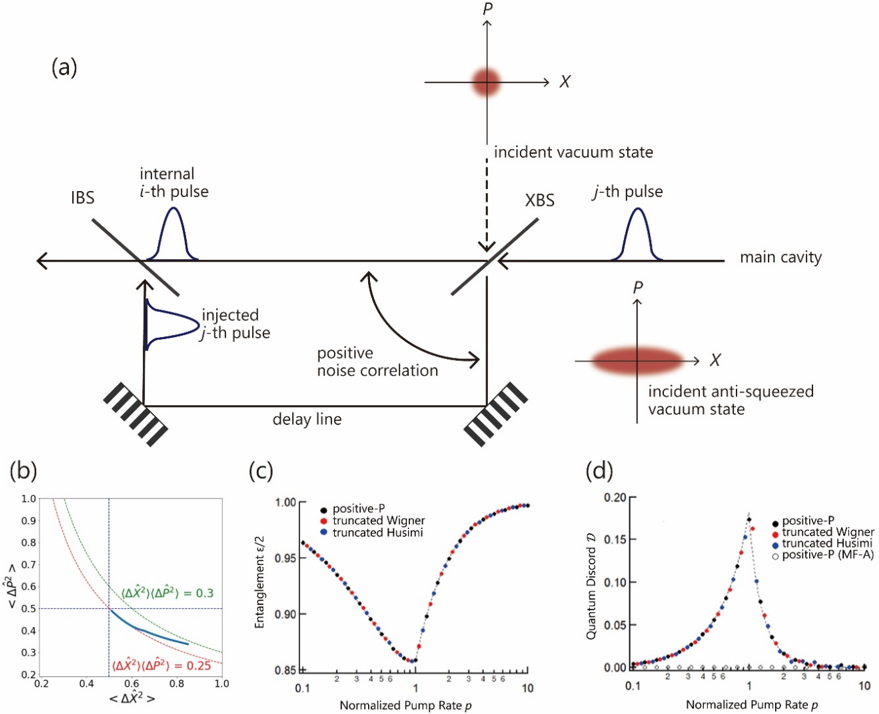## Quantum noise correlation for parallel search The first CIM demonstrated in 2014 uses ( 𝑁𝑁 1 ) optical delay lines to all-to-all couple N-OPO pulses circulating in a ring cavity according to the target Hamiltonian ℋ = ∑𝐽𝐽𝑖𝑖𝑖𝑖 𝑥𝑥 𝑖𝑖 𝑥𝑥 𝑖𝑖 , where 𝑥𝑥 𝑖𝑖 is the in-phase amplitude of ith OPO pulse (see Fig. 1 in [14]). A coupling field Ii is chosen as the gradient of the potential, 𝐼𝐼𝑖𝑖 ∝ -𝜕𝜕ℋ 𝜕𝜕𝑥𝑥 𝑖𝑖 / , where the analog (quadrature) amplitude xi represents the binary spin variable by 𝑥𝑥 𝑖𝑖 = 𝜎𝜎 𝑖𝑖 | 𝑥𝑥 𝑖𝑖 | . When an Ising coupling coefficient 𝐽𝐽 𝑖𝑖𝑖𝑖 between the i -th and j -th OPO pulses is positive (ferromagnetic coupling), an optical delay line realizes in-phase coupling between (internal) i -th and (externally injected) j -th OPO pulse amplitudes (see Fig. 1(a)). The OPO pulses incident upon an extraction beam splitter (XBS) carry anti-squeezed vacuum noise along a generalized coordinate x at below threshold, which produces a positive noise correlation between transmitted and reflected OPO pulses after XBS, while vacuum noise from the XBS open port is negligible compared to the anti-squeezed noise of incident OPO pulse. Positive noise correlation is similarly established between the i -th and j -th OPO pulses after combining the injected j -th OPO pulse and internal i -th OPO pulse at an injection beam splitter (IBS), as shown in Fig. 1(a). When the Ising coupling coefficient 𝐽𝐽 𝑖𝑖𝑖𝑖 is negative (anti-ferromagnetic coupling), the optical delay line realizes an out-of-phase coupling between the i -th and j -th OPO pulse amplitudes. This setup of the optical delay line results in the negative noise correlation between the two OPO pulse amplitudes. Below threshold, each OPO pulse is in an anti-squeezed vacuum state which can be interpreted as a linear superposition (not statistical mixture) of generalized coordinate eigenstates, ∑ 𝒄𝒄𝒏𝒏 | 𝒙𝒙 𝒏𝒏 ⟩ 𝒏𝒏 , if the decoherence effect by linear cavity loss is neglected. In fact, quantum coherence between different | 𝒙𝒙⟩ eigenstates is very robust against small linear loss. [23] Figure 1(b) shows the quantum noise trajectory in 〈∆𝑿𝑿 � 𝟐𝟐 〉 and 〈∆𝑷𝑷 � 𝟐𝟐 〉 phase space. The uncertainty product stays close to the Heisenberg limit, with a very small excess factor of less than 30%, during an entire computation process, which suggests the purity of an OPO state is well maintained. [42] Therefore, the above mentioned positive/negative noise correlation between two OPO pulses depending on ferromagnetic/anti-ferromagnetic coupling, implements a sort of quantum parallel search. That is, if the two OPO pulses couple ferromagnetically, the formed positive quantum noise correlation prefers ferromagnetic phase states | 𝟎𝟎⟩ 𝒊𝒊 | 𝟎𝟎⟩ 𝒊𝒊 and | 𝝅𝝅⟩ 𝒊𝒊 | 𝝅𝝅⟩ 𝒊𝒊 , where | 𝟎𝟎⟩ = ∫ 𝒄𝒄 𝑿𝑿 | 𝒙𝒙⟩𝐝𝐝𝐝𝐝 ∞ 𝟎𝟎 and | 𝝅𝝅⟩ = ∫ 𝒄𝒄 𝑿𝑿 | 𝒙𝒙⟩𝐝𝐝𝐝𝐝 𝟎𝟎 -∞ . If two OPO pulses couple anti- ferromagnetically, the formed negative quantum noise correlation prefers anti-ferromagnetic phase states | 𝟎𝟎⟩ 𝒊𝒊 | 𝝅𝝅⟩ 𝒊𝒊 and | 𝝅𝝅⟩ 𝒊𝒊 | 𝟎𝟎⟩ 𝒊𝒊 . Entanglement and quantum discord between two OPO pulses can be computed to demonstrate such quantum noise correlations. [27][28][29] Figure 1(c) and (d) show the degrees of entanglement and quantum discord versus normalized pump rate 𝒑𝒑 = 𝓔𝓔 𝓔𝓔 𝒅𝒅𝒕𝒕 / , whew 𝓔𝓔 is a pump field amplitude incident upon the nonlinear crystal and 𝓔𝓔 𝒅𝒅𝒕𝒕 is that at the oscillation threshold for a solitary OPO, for an ODL-CIM with N = 2 pulses. [29] In Fig. 1(c), it is shown that Duan-Giedke-Cirac-Zoller entanglement criterion [43] is satisfied at all pump rates. In Fig 1(d), it is shown that Adesso-Datta quantum discord criterion [44] is also satisfied at all pump rate. [29] Both results on entanglement and quantum discord demonstrate maximal quantum noise correlation formed at threshold pump rate p = 1. On the other hand, if a (fictitious) mean-field without quantum noise is assumed to couple two OPO pulses, there exists no quantum correlation below or above threshold, as shown by open circles FIG. 1. (a) An optical delay line couples two OPO pulses in ODL-CIM. [14] (b) Variances 〈∆𝑿𝑿 � 𝟐𝟐 〉 and 〈∆𝑷𝑷 � 𝟐𝟐 〉 in a MFB-CIM with 𝑵𝑵 = 𝟏𝟏𝟏𝟏 OPO pulses. The uncertainty product deviates from the Heisenberg limit by less than 30%. [42] (c) Duan-Giedke-Cirac-Zoller inseparability criterion ( 𝛆𝛆 / 𝟐𝟐 < 𝟏𝟏 ) vs. normalized pump rate 𝒑𝒑 = 𝓔𝓔 𝓔𝓔 𝒅𝒅𝒕𝒕 / . Numerical simulations are performed by the positiveP , truncated-Wigner and truncatedHusimi stochastic differential equations (SDE). The dashed line represents an analytical solution. [29] (d) AdessoDatta quantum discord criterion ( Ɗ > 0) vs. normalized pump rate p . The above three SDEs and the analytical result predict the identical quantum discord, while the mean-field coupling approximation (MF-A) predicts no quantum discord. [29] <details> <summary>Image 1 Details</summary>  ### Visual Description ## Composite Figure: Quantum Optics Experiment and Simulation Results ### Overview The image presents a composite figure comprising a schematic diagram of a quantum optics experiment and three plots comparing simulation results obtained using different theoretical approaches. The experiment involves interacting pulses in a main cavity, and the simulations explore entanglement and quantum discord as a function of normalized pump rate. ### Components/Axes **Figure (a): Schematic Diagram** * **Title:** None explicitly stated, but it represents the experimental setup. * **Components:** * IBS (Input Beam Splitter): Located on the top-left. * XBS (Output Beam Splitter): Located on the top-right. * Main Cavity: The central region where the pulses interact. * Delay Line: At the bottom, connecting the output of IBS to the input of XBS. * Mirrors: Represented by parallel lines. * Pulses: "internal *i*-th pulse" and "injected *j*-th pulse" are shown as Gaussian-like curves. * Incident vacuum state: Shown as a red circle at the top, with axes labeled P and X. * Incident anti-squeezed vacuum state: Shown as a red ellipse at the bottom, with axes labeled P and X. * Positive noise correlation: Indicated by a curved arrow. **Figure (b): Plot of Variance Product** * **X-axis:** `<ΔX²>` (Variance of X) - Ranges from 0.2 to 1.0. * **Y-axis:** `<ΔP²>` (Variance of P) - Ranges from 0.2 to 1.0. * **Curves:** * `(ΔX²)(ΔP²) = 0.3`: Represented by a green dashed line. * `(ΔX²)(ΔP²) = 0.25`: Represented by a blue line. **Figure (c): Plot of Entanglement** * **X-axis:** Normalized Pump Rate *p* - Logarithmic scale from 0.1 to 10. * **Y-axis:** Entanglement ε/2 - Linear scale from 0.85 to 1.00. * **Data Series (Legend - top-right):** * positive-P: Black dots. * truncated Wigner: Red dots. * truncated Husimi: Blue dots. **Figure (d): Plot of Quantum Discord** * **X-axis:** Normalized Pump Rate *p* - Logarithmic scale from 0.1 to 10. * **Y-axis:** Quantum Discord *D* - Linear scale from 0.00 to 0.20. * **Data Series (Legend - top-right):** * positive-P: Black dots. * truncated Wigner: Red dots. * truncated Husimi: Blue dots. * positive-P (MF-A): White dots. ### Detailed Analysis **Figure (a): Schematic Diagram** The diagram illustrates an experimental setup involving two beam splitters (IBS and XBS) and a main cavity. Pulses are injected and interact within the cavity. The delay line provides feedback, and the incident states are either vacuum or anti-squeezed vacuum states. **Figure (b): Plot of Variance Product** The plot shows the relationship between the variances of X and P. The curves represent constant values of the product of these variances. The blue line is below the green line. * The blue line representing `(ΔX²)(ΔP²) = 0.25` starts at approximately `<ΔX²>` = 0.2, `<ΔP²>` = 0.8 and ends at `<ΔX²>` = 0.8, `<ΔP²>` = 0.3. * The green line representing `(ΔX²)(ΔP²) = 0.3` starts at approximately `<ΔX²>` = 0.2, `<ΔP²>` = 0.9 and ends at `<ΔX²>` = 0.9, `<ΔP²>` = 0.3. **Figure (c): Plot of Entanglement** The plot shows how entanglement (ε/2) varies with the normalized pump rate *p*. All three data series (positive-P, truncated Wigner, and truncated Husimi) exhibit a similar trend: * Initially, entanglement is high (close to 1.0) at low pump rates (around 0.1). * As the pump rate increases, entanglement decreases, reaching a minimum around *p* = 1. * Beyond *p* = 1, entanglement increases again, approaching 1.0 at high pump rates (around 10). * The minimum entanglement value is approximately 0.86 at p=1. **Figure (d): Plot of Quantum Discord** The plot shows how quantum discord *D* varies with the normalized pump rate *p*. The data series exhibit the following trends: * All data series start near 0 at low pump rates (around 0.1). * As the pump rate increases, quantum discord increases sharply, reaching a maximum around *p* = 1. * Beyond *p* = 1, quantum discord decreases, approaching 0 at high pump rates (around 10). * The maximum quantum discord value is approximately 0.18 at p=1. ### Key Observations * The schematic diagram illustrates the experimental setup for generating and manipulating quantum states of light. * The variance product plot shows the uncertainty relationship between the variances of X and P. * The entanglement plot shows that entanglement is high at both low and high pump rates, with a minimum around *p* = 1. * The quantum discord plot shows that quantum discord is maximized around *p* = 1 and approaches zero at both low and high pump rates. * The different theoretical approaches (positive-P, truncated Wigner, truncated Husimi, and positive-P (MF-A)) yield similar results for both entanglement and quantum discord, especially at low and high pump rates. ### Interpretation The data suggests that the normalized pump rate *p* plays a crucial role in determining the entanglement and quantum discord of the system. The observed trends indicate that there is an optimal pump rate (around *p* = 1) for maximizing quantum discord, while entanglement is generally high except around this optimal pump rate. The agreement between the different theoretical approaches suggests that the results are robust and not strongly dependent on the specific approximation used. The experiment and simulations demonstrate the generation and manipulation of non-classical states of light, which are essential for quantum information processing and quantum communication. The dip in entanglement and peak in quantum discord around p=1 may indicate a transition in the system's behavior or a change in the dominant physical processes. </details> Note that vacuum noise incident from an open port of XBS (See Fig. 1(a)) creates an opposite noise correlation between the internal and external OPO pulses, so that it always degrades the preferred quantum noise correlation among the two OPO pulses after IBS. Thus, squeezing the vacuum noise at open port of XBS is expected to improve the quantum search performance of an ODL-CIM, which is indeed confirmed in the numerical simulation. 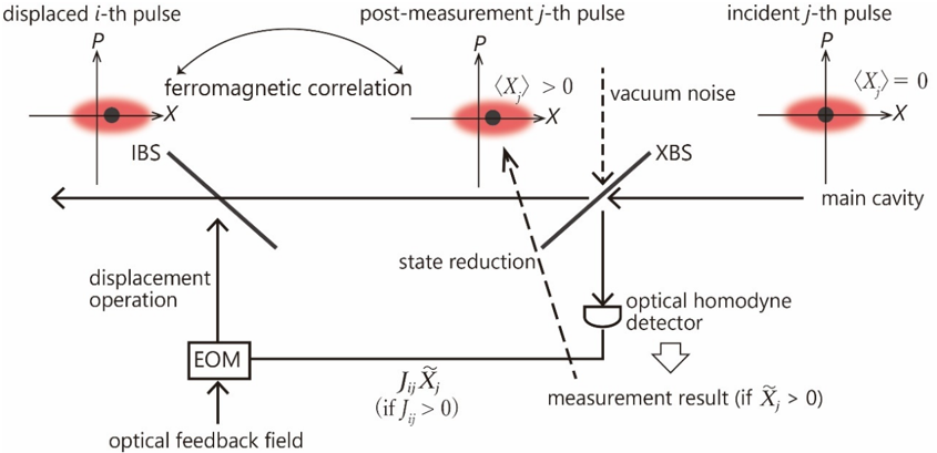[28] The second generation of CIM demonstrated in 2016 employs a measurement-feedback circuit to all-to-all couple the N-OPO pulses (see Fig. 1 of [16]). The (quadrature) amplitude 𝑥𝑥 𝑖𝑖 of a reflected OPO pulse j after XBS is measured by an optical homodyne detector and the measurement result (inferred amplitude) 𝑥𝑥 � 𝑖𝑖 is multiplied against the Ising coupling coefficient Jij and summed over all j pulses in electronic digital circuitry, which produces an overall feedback signal ∑ 𝐽𝐽𝑖𝑖𝑖𝑖 𝑥𝑥 � 𝑖𝑖 𝑖𝑖 for the i -th internal OPO pulse. This analog electrical signal is imposed on the amplitude of a coherent optical feedback signal, which is injected into the target OPO pulse 𝑖𝑖 by IBS. In this MFB-CIM operating below threshold, if a homodyne measurement result 𝑥𝑥 � 𝑖𝑖 is positive and incident vacuum noise from the open port of XBS is negligible, the average amplitude of the internal OPO pulse j is shifted (jumped) to a positive direction by the projection property of such an indirect quantum measurement [45] , as shown in Fig. 2. Depending on the value of a feedback signal 𝐽𝐽 𝑖𝑖𝑖𝑖 𝑥𝑥 � 𝑖𝑖 , we can introduce either positive or negative displacement for the center position of the target OPO pulse i . In this way, depending on the sign of 𝐽𝐽 𝑖𝑖𝑖𝑖 , we can implement either positive correlation or negative correlation between the two average amplitudes 〈𝑥𝑥 𝑖𝑖 〉 and 〈𝑥𝑥 𝑖𝑖 〉 for ferromagnetic or antiferromagnetic coupling, respectively. Note that a MFB-CIM does not produce entanglement among OPO pulses but generates quantum discord if the density operator is defined as an ensemble over many measurement records. [46] A normalized correlation function 𝑁𝑁 = 〈∆𝑋𝑋 � 1 ∆𝑋𝑋 � 2 〉 �〈∆𝑋𝑋 � 1 2 〉〈∆𝑋𝑋 � 2 2 〉 � is an appropriate metric for quantifying such measurement-feedback induced search performance, the degree of which is shown to govern final success probability of MFB-CIM more directly than the quantum discord. In general, a MFB-CIM has a larger normalized correlation function and higher success probability than an ODL-CIM. [46] FIG. 2. Formation of a ferromagnetic correlation between two OPO pulses in MFB-CIM. [15][16] This example illustrates the noise distributions of the two OPO pulses when the Ising coupling is ferromagnetic ( 𝑱𝑱 𝒊𝒊𝒊𝒊 > 𝟎𝟎 ) and the measurement result for the j -th pulse is 𝑿𝑿 � 𝒊𝒊 > 𝟎𝟎 . <details> <summary>Image 2 Details</summary>  ### Visual Description ## Diagram: Optical Feedback Loop with Measurement ### Overview The image is a schematic diagram illustrating an optical feedback loop with measurement, showing the evolution of a light pulse through different stages of interaction and measurement. It depicts the transformation of a displaced i-th pulse, its interaction with a ferromagnetic correlation, the post-measurement j-th pulse, and the incident j-th pulse within a main cavity. The diagram includes optical elements like beam splitters (IBS, XBS), an electro-optic modulator (EOM), and an optical homodyne detector. ### Components/Axes * **Axes:** Each pulse state is represented on a coordinate plane with axes labeled 'P' (vertical) and 'X' (horizontal). * **Pulses:** * "displaced i-th pulse": Located at the top-left. * "post-measurement j-th pulse": Located at the top-center. * "incident j-th pulse": Located at the top-right. * **Optical Elements:** * "IBS": Imbalanced Beam Splitter. * "XBS": Another Beam Splitter. * "EOM": Electro-Optic Modulator. * "optical homodyne detector": Measures the output signal. * **Labels:** * "ferromagnetic correlation": Describes the interaction between the pulses. * "vacuum noise": Indicates noise affecting the beam. * "main cavity": Indicates the location of the incident pulse. * "displacement operation": Describes the operation performed by the EOM. * "state reduction": Describes the effect of the measurement. * "optical feedback field": Indicates the feedback signal. * "measurement result (if X̃j > 0)": Indicates the output of the homodyne detector. * "Jij X̃j (if Jij > 0)": Describes the feedback signal strength. * **Expectation Values:** * "<Xj> > 0": Expectation value of X for the post-measurement pulse. * "<Xj> = 0": Expectation value of X for the incident pulse. ### Detailed Analysis 1. **Displaced i-th pulse (Top-Left):** * Axes: P (vertical), X (horizontal). * A red, roughly circular shape is centered slightly above and to the left of the origin. * A black dot is located near the center of the red shape. 2. **Post-measurement j-th pulse (Top-Center):** * Axes: P (vertical), X (horizontal). * A red, roughly circular shape is centered slightly above and to the right of the origin. * A black dot is located near the center of the red shape. * Label: "<Xj> > 0" indicates a positive expectation value for X. 3. **Incident j-th pulse (Top-Right):** * Axes: P (vertical), X (horizontal). * A red, roughly circular shape is centered at the origin. * A black dot is located at the origin. * Label: "<Xj> = 0" indicates a zero expectation value for X. 4. **Optical Elements and Flow:** * The "displaced i-th pulse" interacts with the "IBS" (Imbalanced Beam Splitter). * An arrow labeled "displacement operation" points from the "EOM" (Electro-Optic Modulator) to the "IBS". * The "post-measurement j-th pulse" interacts with the "XBS". * A dashed arrow labeled "vacuum noise" points towards the "XBS". * A dashed arrow labeled "state reduction" connects the "XBS" to the "optical homodyne detector". * An arrow points from the "optical homodyne detector" to "measurement result (if X̃j > 0)". * An arrow labeled "optical feedback field" points from the "optical homodyne detector" to the "EOM". * The "incident j-th pulse" is located in the "main cavity". * A curved arrow labeled "ferromagnetic correlation" connects the "displaced i-th pulse" to the "post-measurement j-th pulse". ### Key Observations * The diagram illustrates a closed-loop system where the measurement result influences the input pulse via optical feedback. * The expectation value of X changes from zero in the incident pulse to positive after measurement. * The ferromagnetic correlation plays a role in the transformation of the pulse. ### Interpretation The diagram depicts a quantum feedback loop where the state of a light pulse is manipulated and measured. The "displaced i-th pulse" represents an initial state. The interaction with the "IBS" and the "ferromagnetic correlation" modifies the pulse. The "XBS" and "optical homodyne detector" perform a measurement, resulting in "state reduction". The "optical feedback field" then adjusts the "EOM" to influence the subsequent pulses, closing the feedback loop. The change in the expectation value of X from 0 to >0 indicates a change in the pulse's quadrature amplitude due to the measurement and feedback. The condition "if X̃j > 0" suggests that the feedback is conditional on the measurement outcome. This setup could be used for various quantum control and measurement applications, such as squeezing, entanglement generation, or quantum error correction. 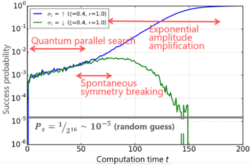</details> In both ODL-CIM and MFB-CIM, anti-squeezed noise below threshold makes it possible to search for a lowest-loss ground state as well as low-loss excited states before the OPO network reaches threshold. The numerical simulation result shown in Fig. 3 demonstrates the three step computation of CIM. [28] We study a 𝑁𝑁 = 16 one-dimensional lattice with a nearest-neighbor antiferromagnetic coupling and periodic boundary condition ( 𝑥𝑥1 = 𝑥𝑥17 ) , for which the two degenerate ground states are |0 ⟩ 1 | 𝜋𝜋⟩2⋯⋯ |0 ⟩ 15 | 𝜋𝜋⟩ 16 and | 𝜋𝜋⟩ 1 |0 ⟩2⋯⋯ | 𝜋𝜋⟩ 15 |0 ⟩ 16 . Before a pump field ℰ is switched on ( 𝑡𝑡 ≤ 0 i n Fig. 3), all OPOs are in vacuum states, for which optical homodyne measurement results provide a simple random guess for each spin and the corresponding success rate is 𝑃𝑃 𝑠𝑠 = 1 2 16 / ∼ 10 -5 as shown by the horizontal solid line in Fig. 3. We assume that vacuum noise incident from the open port of XBS is squeezed by 10 dB in ODL-CIM. When the external pump rate is linearly increased from below to above threshold, the probability of finding the two degenerate ground states is increased by two orders of magnitude above the initial success probability. This enhanced success probability stems from the formation of quantum noise correlation among 16 OPO pulses at below threshold. The probability of finding high-loss excited states, which are not shown in Fig. 3, is deceased to below the initial value. This 'quantum preparation' is rewarded at the threshold bifurcation point. When the pump rate reaches threshold, one of the ground states ( |0 ⟩ 1 | 𝜋𝜋⟩2⋯⋯ | 𝜋𝜋⟩ 16 ) in the case of Fig. 3 is selected as a single oscillation mode, while the other ground state ( | 𝜋𝜋⟩ 1 |0 ⟩2⋯⋯ |0 ⟩ 16 ) as well as all excited states are not selected. This is not a standard single oscillator bifurcation but a collective phenomenon among 𝑁𝑁 = 16 OPO pulses due to the existence of anti-ferromagnetic noise correlation. Above threshold, the probability of finding the selected ground state is exponentially increased, while those of finding the unselected ground state as well as all excited states are exponentially suppressed in a time scale of the order of signal photon lifetime. Such exponential amplification and attenuation of the probabilities is a unique advantage of a gain-dissipative computing machine, which is absent in a standard (unitary gate based) quantum computing system. For example, the Grover search algorithm utilizes a unitary rotation of state vectors and can amplify the target state amplitude only linearly. [25] However, this difference does not mean the computational time of CIM is sub-exponential for hard instances. Recent numerical studies suggest that CIM has an improved but still exponentially scaling time. [30] Note that if we stop increasing the pump rate just above threshold, the probability of finding either one of the ground states is less than 1%. Pitchfork bifurcation followed by exponential amplitude amplification plays a crucial role in realizing high success probability in a short time. For hard instances of combinatorial optimization problems, in which excited states form numerous local minima, the above quantum search alone is not sufficient to guarantee a high success probability. [30] In the next section, another CIM with error correction feedback is introduced to cope with such hard instances. [26] An alternative approach has been recently proposed. [42] If a pump rate is held just below threshold (corresponding to 𝑡𝑡 ∽ 60 in Fig. 3), the lowest-loss ground states and lowloss excited states (fine solutions) have enhanced probabilities while high-loss excited states have suppressed probabilities. By using a MFB-CIM, the optimum as well as good sub-optimal solutions are selectively sampled through an indirect measurement in each round trip of the OPO pulses. This latter approach is particularly attractive if the computational goal is to sample not only optimum solutions but also semi-optimum solutions. FIG. 3. The probabilities of finding two degenerate ground states in ODL-CIM for a one-dimension lattice with nearest-neighbor anti-ferromagnetic coupling and periodic boundary condition ( 𝒙𝒙 𝟏𝟏 = 𝒙𝒙 𝟏𝟏𝟏𝟏 ). [28] Many trajectories produced by the numerical simulation with truncated-Wigner SDE are post-selected by the final state | 𝟎𝟎⟩ 𝟏𝟏 | 𝝅𝝅⟩ 𝟐𝟐⋯⋯ | 𝟎𝟎⟩ 𝟏𝟏𝟏𝟏 | 𝝅𝝅⟩ 𝟏𝟏𝟏𝟏 and ensemble averaged. <details> <summary>Image 3 Details</summary>  ### Visual Description ## Line Chart: Success Probability vs. Computation Time ### Overview The image is a line chart comparing the success probability of two different configurations (sigma_I = up and sigma_I = down) over computation time. The y-axis represents the success probability on a logarithmic scale, and the x-axis represents the computation time. The chart also includes annotations highlighting different phases of the computation, such as "Quantum parallel search," "Exponential amplitude amplification," and "Spontaneous symmetry breaking." A horizontal line indicates the success probability of a random guess. ### Components/Axes * **Title:** Implicit, but the chart depicts "Success probability vs. Computation time." * **X-axis:** * Label: "Computation time t" * Scale: Linear, ranging from 0 to 200, with tick marks at intervals of 50 (0, 50, 100, 150, 200). * **Y-axis:** * Label: "Success probability" * Scale: Logarithmic (base 10), ranging from 10^-6 to 10^0, with tick marks at each power of 10 (10^-6, 10^-5, 10^-4, 10^-3, 10^-2, 10^-1, 10^0). * **Legend:** Located at the top-left of the chart. * Blue line: "σ_I = ↑ (ξ=0.4, r=1.0)" * Green line: "σ_I = ↓ (ξ=0.4, r=1.0)" * **Horizontal Line:** A gray horizontal line is present at approximately 10^-5, labeled "P_s = 1/2^16 ~ 10^-5 (random guess)". * **Annotations:** * "Quantum parallel search" (horizontal arrow, left side) * "Exponential amplitude amplification" (horizontal arrow, right side) * "Spontaneous symmetry breaking" (horizontal arrow, center) ### Detailed Analysis * **Blue Line (σ_I = ↑ (ξ=0.4, r=1.0)):** * Trend: Initially increases slowly during the "Quantum parallel search" phase, then exhibits a rapid, almost exponential increase during the "Exponential amplitude amplification" phase. * Data Points: * At t=0, Success Probability ≈ 10^-6 * At t=50, Success Probability ≈ 10^-3 * At t=100, Success Probability ≈ 10^-2 * At t=150, Success Probability ≈ 10^-1 * At t=200, Success Probability ≈ Approaching 10^0 * **Green Line (σ_I = ↓ (ξ=0.4, r=1.0)):** * Trend: Initially increases slowly during the "Quantum parallel search" phase, then peaks and decreases during the "Spontaneous symmetry breaking" phase. * Data Points: * At t=0, Success Probability ≈ 10^-6 * At t=50, Success Probability ≈ 2 * 10^-3 * At t=100, Success Probability ≈ 3 * 10^-3 * At t=150, Success Probability ≈ 10^-5 * At t=200, Success Probability ≈ 10^-6 * **Horizontal Line (Random Guess):** * Value: Approximately 10^-5. This represents the baseline success probability achieved by a random guess. ### Key Observations * The blue line (σ_I = ↑) shows a significantly higher success probability at later computation times compared to the green line (σ_I = ↓). * The green line (σ_I = ↓) exhibits a peak in success probability around t=100, followed by a decrease, indicating a "Spontaneous symmetry breaking" phenomenon. * Both lines start at the same initial success probability (approximately 10^-6). * The "Exponential amplitude amplification" phase is only evident in the blue line. * The success probability of the blue line surpasses the random guess probability around t=60, while the green line's success probability drops below the random guess probability after t=120. ### Interpretation The chart demonstrates the performance of two different configurations (σ_I = ↑ and σ_I = ↓) in a quantum computation task. The blue line represents a configuration that effectively utilizes "Exponential amplitude amplification" to achieve a high success probability. In contrast, the green line shows a "Spontaneous symmetry breaking" phenomenon, where the success probability decreases after reaching a peak. This suggests that the configuration represented by the blue line is more suitable for this particular computation task. The horizontal line representing the random guess probability provides a baseline for evaluating the effectiveness of the quantum computation. The fact that the blue line significantly exceeds this baseline indicates a successful quantum algorithm, while the green line's eventual drop below the baseline suggests a less effective or even detrimental configuration. </details> ## Destabilization of local minima The measurement-feedback coherent Ising machine has been previously described as a quantum analog device that finishes computation in a classical digital device, in which the amplitude of a selected low energy spin configuration is exponentially amplified. [22][23] During computation, the sign of the measured in-phase component, noted 𝑥𝑥 �𝑖𝑖 with 𝑥𝑥 �𝑖𝑖 ∈ ℝ , is associated with the boolean variable 𝜎𝜎 𝑖𝑖 of an Ising problem (whereas the quadrature-phase component decays to zero). A detailed model of the system's dynamics is given by the master equation of the density operator ρ that is conditioned on measurement results [47][48] which describes the processes of parametric amplification (exchange of one pump photon into two signal photons), saturation (signal photons are converted back into pump photons), wavepacket reduction due to measurement, and feedback injection that is used for implementing the Ising coupling. For the sake of computational tractability, truncated Wigner [28] or the positive-P representation [49] can be used with Itoh calculus for approximating the quantum state to a probability distribution 𝑃𝑃 ( 𝑥𝑥 𝑖𝑖 ) with 𝑃𝑃 ( 𝑥𝑥 𝑖𝑖 ) ≈ 𝑇𝑇𝑇𝑇 [| 𝑥𝑥 𝑖𝑖 ⟩⟨𝑥𝑥 𝑖𝑖 | 𝜌𝜌 ] from which the measured in-phase component 𝑥𝑥 �𝑖𝑖 can be calculated with 𝑥𝑥 �𝑖𝑖 = 〈𝑥𝑥 𝑖𝑖 〉 + 𝛾𝛾𝛾𝛾 𝑖𝑖 where 〈𝑥𝑥 𝑖𝑖 〉 = ∫ 𝑥𝑥 𝑖𝑖 𝑃𝑃 ( 𝑥𝑥 𝑖𝑖 )dx 𝑖𝑖 and 𝛾𝛾 𝑖𝑖 are uncorrelated increments with amplitude 𝛾𝛾 > 0 . Although gain saturation and dissipation can, in principle, induce squeezing and non-Gaussian states [50] that would justify describing the time-evolution of the higher moments of the probability distribution P, it is insightful to limit our description to its first moment (the average 〈𝑥𝑥 𝑖𝑖 〉 ) in order to explain computation achieved by the machine in the classical regime. This approximation is justified when the state of each OPO remains sufficiently close to a coherent state during the whole computation process. In this case, the effect of gain saturation and dissipation on the average 〈𝑥𝑥 𝑖𝑖 〉 can be modeled as a non-linear function 𝑥𝑥 ↦ 𝑓𝑓 ( 𝑥𝑥 ) and the feedback injection is given as 𝛽𝛽 𝑖𝑖 𝛴𝛴 𝑗𝑗 𝐽𝐽 𝑖𝑖𝑗𝑗 𝑔𝑔 ( 〈𝑥𝑥 𝑖𝑖 〉 + 𝛾𝛾𝛾𝛾 𝑗𝑗 ) where 𝑓𝑓 and 𝑔𝑔 are sigmoid functions, 𝐽𝐽 𝑖𝑖𝑗𝑗 the Ising couplings, and 𝛽𝛽 𝑖𝑖 represents the amplitude of the coupling. When the amplitudes | 〈𝑥𝑥 𝑖𝑖 〉 | of OPO signals are much larger that the noise amplitude 𝛾𝛾 , the system can be described by simple differential equations given as (d/dt) 〈𝑥𝑥 𝑖𝑖 〉 = 𝑓𝑓 ( 〈𝑥𝑥 𝑖𝑖 〉 ) + 𝛽𝛽𝛴𝛴 𝑖𝑖 𝑗𝑗 𝑖𝑖𝑖𝑖 𝑔𝑔�〈𝑥𝑥 𝑖𝑖 〉� for which we set 𝛽𝛽 𝑖𝑖 = 𝛽𝛽 , ∀𝑖𝑖 , and it can be shown that the time-evolution of the system is a motion in state space that seeks out minima of a potential function (or Lyapunov function) 𝑉𝑉 given as 𝑉𝑉 = 𝑉𝑉 𝑏𝑏 ( 𝒚𝒚 ) + 𝛽𝛽𝐻𝐻 ( 𝒚𝒚 ) where 𝑉𝑉 𝑏𝑏 is a bistable potential with 𝑉𝑉 𝑏𝑏 ( 𝒚𝒚 ) = -𝛴𝛴𝑖𝑖∫ 𝑓𝑓 ( 𝑔𝑔 -1 ( 𝑦𝑦 ))d 𝑦𝑦 and 𝐻𝐻 ( 𝒚𝒚 ) = - (1/2) 𝛴𝛴 𝑖𝑖𝑖𝑖 𝑗𝑗 𝑖𝑖𝑖𝑖 𝑦𝑦 𝑖𝑖 𝑦𝑦 𝑖𝑖 is the extension of the Ising Hamiltonian in the real space with 𝑦𝑦 𝑖𝑖 = 𝑔𝑔 ( 〈𝑥𝑥 𝑖𝑖 〉 ) . [21][51] The connection between such nonlinear differential equations and the Ising Hamiltonian has been used in various models such as in the 'soft' spin description of frustrated spin systems [52] or the Hopfield-Tank neural networks [51] for solving NPhard combinatorial optimization problems. Moreover, an analogy with the mean-field theory of spin glasses can be made by recognizing that the steady-states of these nonlinear equations correspond to the solution of the 'naive' Thouless-Anderson-Palmer (TAP) equations [53] which arise from the meanfield description of Sherrington-Kirkpatrick spin glasses in the limit of large number of spins 𝑁𝑁 and are given as 〈𝜎𝜎 𝑖𝑖 〉 = tanh((1/ 𝑇𝑇 ) 𝛴𝛴 𝑖𝑖 𝐽𝐽 𝑖𝑖𝑖𝑖 〈𝜎𝜎 𝑖𝑖 〉 ) with 〈𝜎𝜎 𝑖𝑖 〉 the thermal average at temperature 𝑇𝑇 of the Ising spin (by setting 𝑓𝑓 ( 𝑥𝑥 ) = 𝑎𝑎 tanh( 𝑥𝑥 ) and 𝑔𝑔 ( 𝑥𝑥 ) = 𝑥𝑥 ). This analogy suggests that the parameter 𝛽𝛽 can be interpreted as inverse temperature in the thermodynamic limit when the Onsager reaction term is discarded. [53] At 𝛽𝛽 = 0 ( 𝑇𝑇 → ∞ ) , the only stable state of the CIM is 〈𝑥𝑥 𝑖𝑖 〉 = 0 , for which any spin configuration is equiprobable, whereas at 𝛽𝛽 → ∞ ( 𝑇𝑇 = 0) , the state remains trapped for an infinite time in local minima. We will discuss in much more detail analogies between CIM dynamics and TAP equations, and also belief and survey propagation, in the special case of the SK model in the next section. 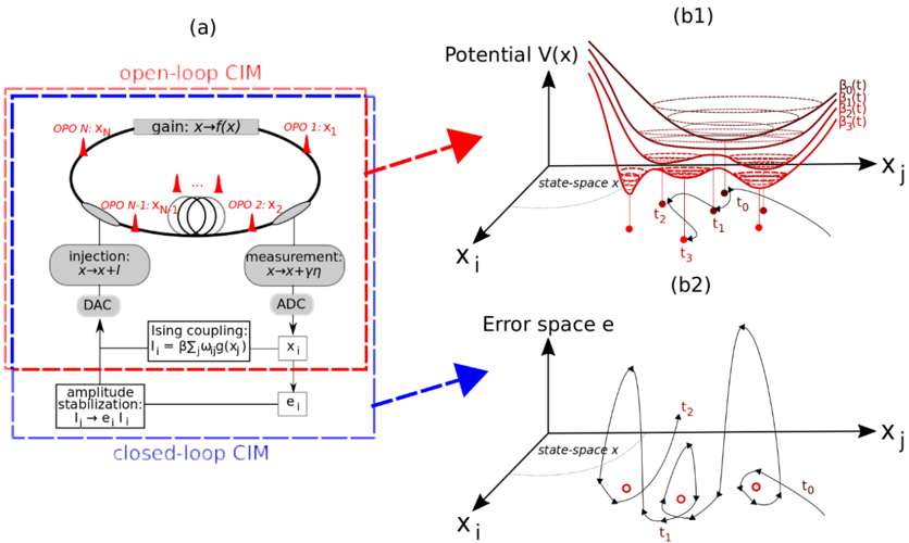In the case of spin glasses, statistical analysis of TAP equations suggests that the free energy landscape has an exponentially large number of solutions near zero temperature [54] and we can expect similar statistics for the potential 𝑉𝑉 when 𝛽𝛽 → ∞ . In order to reduce the probability of the CIM to get trapped in one of the local minima of 𝑉𝑉 , it has been proposed to gradually increase 𝛽𝛽 , the coupling strength, during computation. [16] This heuristic, that we call open-loop CIM in the following, is similar to mean-field annealing [55] and consists in letting the system seeks out minima of a potential 𝑦𝑦 𝑖𝑖 function 𝑉𝑉 that is gradually transformed from monostable to multi-stable (see Fig. 4(a) and (b1)). Contrarily to the quantum adiabatic theorem [56] or the convergence theorem of simulated annealing, [57] there is however no guarantee that a sufficiently slow deformation of 𝑉𝑉 will ensure convergence to the configuration of lowest Ising Hamiltonian. In fact, linear stability analysis suggests on the contrary that the first state other than vacuum state ( 〈𝑥𝑥 𝑖𝑖 〉 = 0 , ∀ 𝑖𝑖 ) to become stable as 𝛽𝛽 is increased does not correspond to the ground-state. Moreover, added noise 𝛾𝛾 𝑖𝑖 may not be sufficient for ensuring convergence: [58] it is possible to seek for global convergence to the minima of the potential 𝑉𝑉 by reducing gradually the amplitude of the noise 𝛾𝛾 (with 𝛾𝛾 ( 𝑡𝑡 ) 2 ~ 𝑐𝑐 /log(2 + 𝑡𝑡 ) and 𝑐𝑐 real constant sufficiently large, [59] but the global minima of the potential 𝑉𝑉 ( 𝑦𝑦 ) do not generally correspond to that of the Ising Hamiltonians 𝐻𝐻 ( 𝝈𝝈 ) at a fixed 𝛽𝛽 . [13][21] This discrepancy between the minima of the potential 𝑉𝑉 and Ising Hamiltonian H can be understood by noting that the field amplitudes 〈𝑥𝑥 𝑖𝑖 〉 are not all equal (or homogeneous) at the steady-state, that is 〈𝑥𝑥 𝑖𝑖 〉 = 𝜎𝜎 𝑖𝑖√𝑎𝑎 + 𝛿𝛿 𝑖𝑖 where 𝛿𝛿 𝑖𝑖 is the variation of the i -th OPO amplitude with 𝛿𝛿 𝑖𝑖 ≠ 𝛿𝛿 𝑖𝑖 and √𝑎𝑎 a reference amplitude defined such that 𝛴𝛴 𝑗𝑗 𝛿𝛿 𝑗𝑗 = 0 . Because of the heterogeneity in amplitude, the minima of 𝑉𝑉 ( 〈𝑥𝑥〉 ) = 𝑉𝑉 ( 𝝈𝝈√𝑎𝑎 + 𝜹𝜹 ) do not correspond to that of 𝐻𝐻 ( 𝝈𝝈 ) in general. Consequently, it is necessary in practice to run the open-loop CIM from multiple initial conditions in order to find the ground-state configuration. FIG. 4. (a) Schematic representation of the open- and closed-loop measurement-feedback coherent Ising machine which computational principle in the mean-field approximation are based on two different types of <details> <summary>Image 4 Details</summary>  ### Visual Description ## Diagram: Open-loop and Closed-loop CIM with Potential and Error Space Visualizations ### Overview The image presents a schematic diagram of both open-loop and closed-loop Coherent Ising Machines (CIMs), accompanied by visualizations of the potential landscape and error space associated with the system's dynamics. The diagram is divided into three main sections: (a) showing the CIM configurations, (b1) illustrating the potential V(x), and (b2) illustrating the error space e. ### Components/Axes #### Section (a): CIM Configurations * **Title:** (a) * **Sub-title:** open-loop CIM (enclosed in a dashed red box) * **Sub-title:** closed-loop CIM (enclosed in a dashed blue box) * **Components within the Open-loop CIM:** * A circular loop representing the optical path. * OPO N: XN (Optical Parametric Oscillator N, with output XN) * gain: x→f(x) (Gain element, transforming input x to f(x)) * OPO 1: X1 (Optical Parametric Oscillator 1, with output X1) * OPO N-1: XN/1 (Optical Parametric Oscillator N-1, with output XN/1) * OPO 2: X2 (Optical Parametric Oscillator 2, with output X2) * injection: x→x+l (Injection element, adding l to input x) * measurement: x→x+γη (Measurement element, transforming input x to x+γη) * DAC (Digital-to-Analog Converter) * ADC (Analog-to-Digital Converter) * Ising coupling: Ii = βΣjωijg(xj) (Ising coupling element, calculating Ii based on coupling strength β, weights ωij, and function g(xj)) * **Components within the Closed-loop CIM:** * amplitude stabilization: Ii→eiIi (Amplitude stabilization element, transforming Ii to eiIi) * ei (Error signal) #### Section (b1): Potential V(x) * **Title:** (b1) * **Graph Title:** Potential V(x) * **Axes:** * Vertical axis: Potential V(x) * Horizontal axis: Xj * Depth axis: Xi * state-space x (label near the Xj and Xi axes) * **Curves:** * Multiple potential energy curves, resembling potential wells, in red. * Dashed lines representing different energy levels: β0(t), β1(t), β2(t), β3(t) * Trajectory of a particle moving through the potential landscape, marked with points t0, t1, t2, t3. #### Section (b2): Error space e * **Title:** (b2) * **Graph Title:** Error space e * **Axes:** * Vertical axis: e (Error space) * Horizontal axis: Xj * Depth axis: Xi * state-space x (label near the Xj and Xi axes) * **Curves:** * Trajectory of the system in error space, showing oscillations and convergence. * Points t0, t1, t2, t3 along the trajectory. * Red circles indicating stable points. ### Detailed Analysis or ### Content Details #### Section (a): CIM Configurations The open-loop CIM consists of a ring of optical parametric oscillators (OPOs) with gain, injection, and measurement components. The closed-loop CIM adds amplitude stabilization and feedback based on an error signal. The Ising coupling element calculates the interaction between the oscillators. #### Section (b1): Potential V(x) The potential energy landscape shows multiple potential wells, representing different energy states. The particle trajectory illustrates how the system evolves over time, moving between these states. The energy levels β0(t), β1(t), β2(t), β3(t) represent different energy thresholds. The trajectory starts at t0, moves to t1, t2, and then t3. #### Section (b2): Error space e The error space visualization shows the system's trajectory as it converges towards stable points. The trajectory starts at t0, moves to t1, t2, and then t3. The red circles indicate stable states where the error is minimized. ### Key Observations * The open-loop CIM lacks feedback control, while the closed-loop CIM incorporates feedback for amplitude stabilization. * The potential energy landscape in (b1) illustrates the energy states and transitions of the system. * The error space visualization in (b2) shows how the system converges towards stable solutions. ### Interpretation The diagram illustrates the fundamental principles of Coherent Ising Machines (CIMs) and their dynamics. The open-loop CIM represents a basic configuration, while the closed-loop CIM incorporates feedback control to improve stability and performance. The potential energy landscape provides a visual representation of the system's energy states and transitions, while the error space visualization shows how the system converges towards stable solutions. The addition of feedback in the closed-loop CIM allows for better control and stabilization of the system, leading to improved performance in solving optimization problems. </details> dynamical systems: gradual deformation of a potential function 𝑽𝑽 (b1) and chaotic-like dynamics (b2), respectively. Because the benefits of using an analog state for finding the ground-state spin configurations of the Ising Hamiltonian is offset by the negative impact of its improper mapping to the potential function 𝑉𝑉 , we have proposed to utilize supplementary dynamics that are not related to the gradient descent of a potential function but ensure that the global minima of 𝐻𝐻 are reached rapidly. In Ref [26], an error correction feedback loop has been proposed whose role is to reduce the amplitude heterogeneity 𝛿𝛿 𝑖𝑖 by forcing squared amplitudes 〈𝑥𝑥 𝑖𝑖 〉 2 to become all equal to a target value 𝑎𝑎 , thus forcing the measurement-feedback coupling { 𝛴𝛴 𝑖𝑖 𝐽𝐽 𝑖𝑖𝑖𝑖 𝑔𝑔 ( 〈𝑥𝑥 𝑖𝑖 〉 )} 𝑖𝑖 to be colinear with the Ising internal field 𝒕𝒕 with ℎ𝑖𝑖 = 𝛴𝛴 𝑖𝑖 𝐽𝐽 𝑖𝑖𝑖𝑖 𝜎𝜎 𝑖𝑖 . This can notably be achieved by introducing error signals, noted 𝑒𝑒 𝑖𝑖 with 𝑒𝑒 𝑖𝑖 ∈ ℝ , that modulate the coupling strength 𝛽𝛽 𝑖𝑖 (or 'effective' inverse temperature) of the i -th OPO such that 𝛽𝛽 𝑖𝑖 = 𝛽𝛽𝑒𝑒 𝑖𝑖 ( 𝑡𝑡 ) and the time-evolution of 𝑒𝑒 𝑖𝑖 given as (d/dt) 𝑒𝑒 𝑖𝑖 = -𝜉𝜉 ( 𝑔𝑔 ( 〈𝑥𝑥 𝑖𝑖 〉 ) 2 -𝑎𝑎 ) 𝑒𝑒 𝑖𝑖 where 𝜉𝜉 is the rate of change of error variables with respect to the signal field. This mode of operation is called closed-loop CIM and can be realized experimentally by simulating the dynamics of the error variables 𝑒𝑒 𝑖𝑖 using the FPGA used in the measurement-feedback CIM for calculation of the Ising coupling [16] (see Fig. 4(a)). Note that the concept of amplitude heterogeneity error correction has also been recently proposed in [20] and extended to other systems such as the XY model. 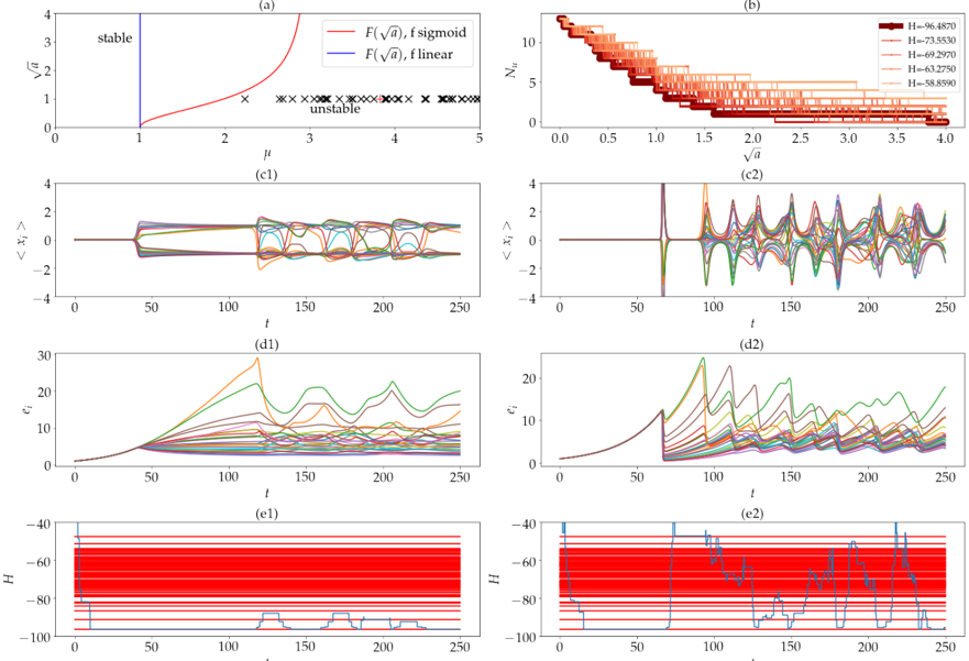[20][60][61] In the case of the closed-loop CIM, the system exhibits steady-states only at the local minima of 𝐻𝐻 . [26] The stability of each local minima can be controlled by setting the target amplitude a as follows: the dimension of the unstable manifold 𝑁𝑁 𝑢𝑢 (where 𝑁𝑁 𝑢𝑢 is the number of unstable directions) at fixed points corresponding to local minima 𝝈𝝈 of the Ising Hamiltonian is equal to the number of eigenvalues 𝜇𝜇 𝑖𝑖 ( 𝝈𝝈 ) that are such that 𝜇𝜇 𝑖𝑖 ( 𝝈𝝈 ) > 𝐹𝐹 ( 𝑎𝑎 ) where 𝜇𝜇 𝑖𝑖 ( 𝝈𝝈 ) are the eigenvalues of the matrix { 𝐽𝐽 𝑖𝑖𝑖𝑖 /| ℎ𝑖𝑖 |} 𝑖𝑖 (with internal field ℎ𝑖𝑖 = 𝛴𝛴 𝑖𝑖 𝐽𝐽 𝑖𝑖𝑖𝑖 𝜎𝜎 𝑖𝑖 ) and 𝐹𝐹 a function shown in Fig. 5(a). The parameter 𝑎𝑎 can be set such that all local minima (including the ground-state) are unstable such that the dynamics cannot become trapped in any fixed point attractors. The system then exhibits chaotic dynamics that explores successively local minima. Note that the use of chaotic dynamics for solving Ising problems has been discussed previously, [24][62] notably in the context of neural networks, and it has been argued that chaotic fluctuations may possess better properties than Brownian noise for escaping from local minima traps. In the case of the closed-loop CIM, the chaotic dynamics is not merely used as a replacement to noise. Rather, the interaction between nonlinear gain saturation and error-correction allows a greater reduction of the unstable manifold dimension of states associated with lower Ising Hamiltonian (see Fig. 5(b)). Comparison between Fig. 5(c1,d1,e1) and (c2,d2,e2) indeed shows that the dynamics of closed-loop CIM samples more efficiently from lower-energy states when the gain saturation is nonlinear compared to the case without nonlinear saturation, respectively. <details> <summary>Image 5 Details</summary>  ### Visual Description ## Chart/Diagram Type: Multi-Panel Figure ### Overview The image is a multi-panel figure consisting of six subplots, arranged in a 3x2 grid. The subplots display various relationships between parameters, including stability analysis, population dynamics, and energy levels. The figure explores the behavior of a system under different conditions, likely related to a physical or biological model. ### Components/Axes **Panel (a): Stability Diagram** * **X-axis:** μ (mu), ranging from 0 to 5. * **Y-axis:** √a (square root of a), ranging from 0 to 4. * **Curves:** * Red line: F(√a), f sigmoid * Blue line: F(√a), f linear * **Regions:** * "stable" region to the left of the blue line (μ ≈ 1). * "unstable" region indicated by black 'x' marks to the right of the red line. **Panel (b): Population Dynamics** * **X-axis:** √a (square root of a), ranging from 0 to 4. * **Y-axis:** N_u, ranging from 0 to 12. * **Curves:** Multiple lines representing different values of H (energy), ranging from -96.4870 to -58.8590. The lines are colored in shades of brown, with darker shades representing lower H values. * H = -96.4870 (darkest brown) * H = -73.5530 * H = -69.2970 * H = -63.2750 * H = -58.8590 (lightest brown) **Panel (c1) and (c2): Time Series of <x_i>** * **X-axis:** t (time), ranging from 0 to 250. * **Y-axis:** <x_i>, ranging from -4 to 4. * **Curves:** Multiple lines, each representing a different instance or component of the system. **Panel (d1) and (d2): Time Series of e_i** * **X-axis:** t (time), ranging from 0 to 250. * **Y-axis:** e_i, ranging from 0 to 30. * **Curves:** Multiple lines, each representing a different instance or component of the system. **Panel (e1) and (e2): Time Series of H** * **X-axis:** t (time), ranging from 0 to 250. * **Y-axis:** H (energy), ranging from -100 to -40. * **Curves:** * Multiple red lines clustered around -60. * A single blue line showing fluctuations in energy. ### Detailed Analysis or ### Content Details **Panel (a): Stability Diagram** * The blue line (F(√a), f linear) is a vertical line at μ ≈ 1, indicating a sharp transition to instability. * The red line (F(√a), f sigmoid) curves upward, showing that the system becomes unstable at lower √a values as μ increases. * The region to the left of the blue line is labeled "stable," while the region to the right of the red line is marked with "x" symbols and labeled "unstable." **Panel (b): Population Dynamics** * The number of populations, N_u, decreases as √a increases. * The different H values (energy levels) influence the rate of decrease in N_u. Lower H values (darker brown lines) show a steeper decrease in N_u as √a increases. * The lines show a step-wise decrease, suggesting discrete population levels. **Panel (c1) and (c2): Time Series of <x_i>** * In panel (c1), the lines start at approximately 0 and then diverge around t=50, oscillating before settling to a value between -2 and 2. * In panel (c2), the lines start at approximately 0 and then diverge around t=50, oscillating with larger amplitudes than in (c1). **Panel (d1) and (d2): Time Series of e_i** * In both panels, the lines start at approximately 0 and then increase rapidly around t=50. * The lines in panel (d1) show a more gradual increase and then oscillate. * The lines in panel (d2) show a more rapid increase and larger oscillations. **Panel (e1) and (e2): Time Series of H** * In both panels, there are multiple red lines clustered around -60. * The blue line in panel (e1) shows a few drops in energy around t=125 and t=175. * The blue line in panel (e2) shows more frequent and larger fluctuations in energy. ### Key Observations * Panel (a) shows the stability of the system based on parameters μ and √a, with a clear distinction between stable and unstable regions. * Panel (b) illustrates how the population dynamics (N_u) are affected by √a and the energy level (H). * Panels (c1) and (c2) show the time evolution of <x_i> under two different conditions. * Panels (d1) and (d2) show the time evolution of e_i under two different conditions. * Panels (e1) and (e2) show the time evolution of H under two different conditions. ### Interpretation The figure presents a comprehensive analysis of a system's behavior, exploring its stability, population dynamics, and energy levels. The stability diagram in panel (a) defines the conditions under which the system remains stable or becomes unstable. Panel (b) shows how the population dynamics are influenced by the system's parameters. Panels (c), (d), and (e) show the time evolution of different variables under two different conditions, allowing for a comparison of the system's behavior. The differences between the left and right columns (c1/c2, d1/d2, e1/e2) likely represent different parameter settings or initial conditions, leading to distinct dynamic behaviors. The clustering of red lines in panels (e1) and (e2) suggests a common energy level, while the blue line indicates fluctuations or transitions in the system's energy state. </details> t FIG. 5. (a) Stability of local minima in the space { √𝒂𝒂 , 𝝁𝝁 } in the case of f sigmoid and linear, i.e., with and without gain saturation, respectively. The red and black crosses correspond to the maximum values of 𝝁𝝁 𝒊𝒊 ( 𝝈𝝈 ) for the ground-state and excited states, respectively, of an example spin-glass instance with 𝑵𝑵 = 𝟐𝟐𝟏𝟏 spins. (b) Dimension of the unstable manifold vs. the target amplitude √𝒂𝒂 for the various local minima with Ising Hamiltonian H shown by the color gradient in the case of f sigmoid. (c1), (d1), and (e1) show the time-evolution of in-phase components 〈𝒙𝒙 𝒊𝒊 〉 , error variables 𝒆𝒆 𝒊𝒊 , and Ising Hamiltonian in the case of f sigmoid. (c2,d2,e2) same as (c1,d1,e1) in the case of f linear. In (e1,e2), the red lines show the Ising Hamiltonian of the local minima. Generally, the asymmetric coupling between in-phase components and error signals possibly results in the creation of limit cycles or chaotic attractors that can trap the dynamics in a region that does not include the global minima of the Ising Hamiltonian. A possible approach to prevent the system from getting trapped in such non-trivial attractors is to dynamically modulate the target amplitude such that the rate of divergence of the velocity vector field remains positive. [26] This implies that volumes along the flow never contract which, in turn, prevents the existence of any attractor. 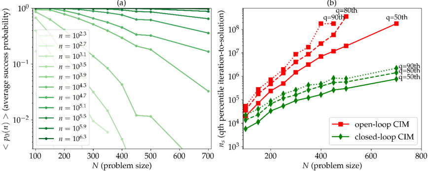Figure 6(a) shows that the closed-loop CIM can find the ground-states of Sherrington- Kirkpatrick spin glass problems with high success probability using a single run even for larger system size. Moreover, the correction of amplitude heterogeneity allows for a significant decrease in the time-to-solution compared to the open-loop case which is evaluated by calculating the number of cavity round-trip of the OPO pulses, called number of iterations and noted 𝑛𝑛 𝑠𝑠 , to find the groundstate configurations with 99% success probability (see Fig. 6(b)). Because there is no theoretical guarantee that the system will find configuration with Ising Hamiltonian at a ratio of the ground-state after a given computational time and the closed-loop CIM is thus classified as a heuristic method. In order to compare it with other state-of-the-art heuristics, the proposed scheme has been applied to solving instances of standard benchmarks (such as the G-set) by comparing time-to-solutions for reaching a predefined target such as the ground-state energy, if it is known, or the smallest energy known (i.e., published), otherwise. The amplitude heterogeneity error correction scheme can in particular find lower energy configurations of MAXCUT problems from the G-set of similar quality as the state-of-the-art solver, called BLS [63] (see the supplementary material of ref [26] for details). Moreover, the averaged time-to-solution obtained using the proposed scheme are similar to the ones obtained using BLS when simulated on a desktop computer, but are expected to be 100-1000 times smaller in the case of an implementation on the coherent Ising machine. FIG. 6. (a) Success probability 〈𝒑𝒑 𝟎𝟎 ( 𝒏𝒏 ) 〉 of finding the ground-state configuration after 𝒏𝒏 iterations of a single run averaged over 100 randomly generated Sherrington-Kirkpatrick spin glass instances and (b) 50th, 80th, and 90th percentiles of the iteration-to-solution distribution where ns of a given instance is given as 𝒏𝒏 𝒔𝒔 = 𝐦𝐦𝐦𝐦𝐦𝐦 𝐦𝐦 { 𝒏𝒏 𝒔𝒔 ( 𝒏𝒏 )} and 𝒏𝒏 𝒔𝒔 ( 𝒏𝒏 ) = 𝒏𝒏 𝐥𝐥𝐥𝐥𝐥𝐥 ( 𝟏𝟏 - 𝟎𝟎 . 𝟗𝟗𝟗𝟗 ) / 𝐥𝐥𝐥𝐥𝐥𝐥 ( 𝟏𝟏 - 𝒑𝒑 𝟎𝟎 ( 𝒏𝒏 )) for the open-loop (in red) and closed-loop CIM (in green). <details> <summary>Image 6 Details</summary>  ### Visual Description ## Chart: Success Probability and Iteration-to-Solution vs. Problem Size ### Overview The image presents two plots side-by-side, labeled (a) and (b). Plot (a) shows the average success probability as a function of problem size for different values of 'n'. Plot (b) shows the qth percentile iteration-to-solution as a function of problem size for open-loop and closed-loop CIM. ### Components/Axes **Plot (a):** * **Title:** (a) * **X-axis:** N (problem size), linear scale from 100 to 700 in increments of 100. * **Y-axis:** <p₀(n)> (average success probability), logarithmic scale from 10⁻² to 10⁰. * **Legend:** Located on the left side of the plot. Each line represents a different value of 'n': * Lightest Green: n = 10²·³ * n = 10²·⁷ * n = 10³·¹ * n = 10³·⁵ * n = 10³·⁹ * n = 10⁴·³ * n = 10⁴·⁷ * n = 10⁵·¹ * n = 10⁵·⁵ * n = 10⁵·⁹ * Darkest Green: n = 10⁶·³ **Plot (b):** * **Title:** (b) * **X-axis:** N (problem size), linear scale from 0 to 800 in increments of 200. * **Y-axis:** nₛ (qth percentile iteration-to-solution), logarithmic scale from 10³ to 10⁸. * **Legend:** Located at the bottom of the plot. * Red squares: open-loop CIM * Green diamonds: closed-loop CIM * **Percentiles:** q = 50th, 80th, 90th are marked for both open-loop and closed-loop CIM. ### Detailed Analysis **Plot (a): Average Success Probability** The plot shows the average success probability decreases as the problem size (N) increases. The rate of decrease varies depending on the value of 'n'. * **n = 10²·³:** The success probability starts near 1 and decreases gradually to approximately 0.01 as N increases from 100 to 700. * **n = 10²·⁷:** The success probability starts near 1 and decreases gradually to approximately 0.005 as N increases from 100 to 700. * **n = 10³·¹:** The success probability starts near 1 and decreases gradually to approximately 0.002 as N increases from 100 to 700. * **n = 10³·⁵:** The success probability starts near 1 and decreases gradually to approximately 0.001 as N increases from 100 to 700. * **n = 10³·⁹:** The success probability starts near 1 and decreases gradually to approximately 0.0005 as N increases from 100 to 700. * **n = 10⁴·³:** The success probability starts near 1 and decreases gradually to approximately 0.0002 as N increases from 100 to 700. * **n = 10⁴·⁷:** The success probability starts near 1 and decreases gradually to approximately 0.0001 as N increases from 100 to 700. * **n = 10⁵·¹:** The success probability starts near 1 and decreases gradually to approximately 0.00005 as N increases from 100 to 700. * **n = 10⁵·⁵:** The success probability starts near 1 and decreases gradually to approximately 0.00002 as N increases from 100 to 700. * **n = 10⁵·⁹:** The success probability starts near 1 and decreases gradually to approximately 0.00001 as N increases from 100 to 700. * **n = 10⁶·³:** The success probability remains close to 1 across the entire range of N values. **Plot (b): Qth Percentile Iteration-to-Solution** The plot shows the qth percentile iteration-to-solution increases as the problem size (N) increases. Open-loop CIM generally requires more iterations than closed-loop CIM for the same problem size and percentile. * **Open-loop CIM (Red):** * q = 50th (solid line): Increases from approximately 10⁴ at N=100 to approximately 2 * 10⁶ at N=700. * q = 80th (dashed line): Increases from approximately 2 * 10⁴ at N=100 to approximately 6 * 10⁶ at N=500. * q = 90th (dotted line): Increases from approximately 3 * 10⁴ at N=100 to approximately 10⁷ at N=500. * **Closed-loop CIM (Green):** * q = 50th (solid line): Increases from approximately 10⁴ at N=100 to approximately 2 * 10⁵ at N=700. * q = 80th (dashed line): Increases from approximately 2 * 10⁴ at N=100 to approximately 3 * 10⁵ at N=500. * q = 90th (dotted line): Increases from approximately 3 * 10⁴ at N=100 to approximately 4 * 10⁵ at N=500. ### Key Observations * In plot (a), as 'n' increases, the average success probability becomes less sensitive to changes in problem size (N). * In plot (b), the number of iterations required to reach a solution increases with problem size for both open-loop and closed-loop CIM. * Open-loop CIM generally requires significantly more iterations than closed-loop CIM to reach a solution. * Higher percentiles (q = 80th, 90th) require more iterations than lower percentiles (q = 50th). ### Interpretation The plots demonstrate the trade-offs between success probability and the number of iterations required to solve a problem using different CIM approaches. Plot (a) shows that for larger values of 'n', the success probability remains high even for larger problem sizes. However, plot (b) shows that closed-loop CIM generally requires fewer iterations to reach a solution compared to open-loop CIM, suggesting it is more efficient. The choice between open-loop and closed-loop CIM, and the selection of 'n', would depend on the specific requirements of the problem, balancing the need for high success probability with the desire for efficient computation. </details> ## Qualitative parallels between the CIM, belief propagation and survey propagation As we have noted above, the CIM approach to solving combinatorial optimization problems over binary valued spin variables 𝜎𝜎 𝑖𝑖 = ±1 can be understood in terms of two key steps. First, in the classical limit of the CIM, the binary valued spin variables 𝜎𝜎 𝑖𝑖 are promoted to analog variables 𝑥𝑥 𝑖𝑖 reflecting the (quadrature) amplitude of the 𝑖𝑖 𝑡𝑡ℎ OPO mode and the classical CIM dynamics over the variables 𝑥𝑥 𝑖𝑖 can be described by a nonlinear differential equation (Eq. 1). Second, in a more quantum regime, the CIM implements a quantum parallel search over this space that focuses quantum amplitudes on the ground state. A qualitatively similar two step approach of state augmentation and then parallel search has also been pursued in statistics and computer science based approaches to combinatorial optimization, specifically in the forms of algorithms known as belief propagation (BP) [64] and survey propagation (SP). [65] Here we outline similarities and differences between CIM, BP and SP. Forming a bridge between these fields can help progress through the cross-pollination of ideas in two distinct ways. First, our theoretical understanding of BP and SP may provide further tools, beyond the dynamical systems theory approaches described above, to develop a theoretical understanding of CIM dynamics. Second, differences between CIM dynamics and BP and SP dynamics may provide further inspiration for the rational engineering design of modified CIM dynamics that could lead to improved performance. Indeed there is a rich literature connecting BP and SP to other ideas in statistical physics, such as the Bethe approximation, the replica method, the cavity method, and TAP equations. [66][67][68][69][70] It may also be interesting to explore connections between these ideas and the theory of CIM dynamics. We begin by discussing BP, which is a general method for computing the marginal distribution 𝑃𝑃 ( 𝜎𝜎 𝑖𝑖 ) = ∑ 𝑃𝑃 ( 𝜎𝜎1 , … , 𝜎𝜎 / 𝑖𝑖 𝜎𝜎 𝑁𝑁 ) from a complex joint distribution over N variables 𝜎𝜎 𝑖𝑖 for 𝑗𝑗 = 1… 𝑁𝑁 . Here the sum over 𝜎𝜎 / 𝑖𝑖 denotes a sum over all variables 𝜎𝜎 𝑖𝑖 for 𝑗𝑗 ≠ 𝑖𝑖 . For binary spin variables 𝜎𝜎 𝑖𝑖 = ±1 , and for general joint distributions 𝑃𝑃 ( 𝜎𝜎1 , … 𝜎𝜎 𝑁𝑁 ) , the computation of this marginal distribution is intractable, as it involves a sum over 𝑂𝑂 (2 𝑁𝑁 ) spin configurations. However, consider the case where the joint distribution 𝑃𝑃 ( 𝜎𝜎1 , … 𝜎𝜎 𝑁𝑁 ) has a locally factorizable structure of the form 𝑃𝑃 ( 𝜎𝜎1 , … 𝜎𝜎 𝑁𝑁 ) = 1 𝑍𝑍 ∏ 𝜓𝜓 𝑎𝑎 𝑃𝑃 𝑎𝑎=1 ( 𝜎𝜎 𝑎𝑎 ). Here we have 𝑃𝑃 interaction terms indexed by 𝑎𝑎 = 1, … , 𝑃𝑃 , and each interaction term, or factor 𝜓𝜓 𝑎𝑎 depends on a subset of the spins denoted by 𝜎𝜎 𝑎𝑎 . Note that a parameter 'a' represents an interaction term in this section, while it means a target intensity in the previous section. For example, in the case of Ising spin systems with pairwise interactions at inverse temperature 𝛽𝛽 , each subset 𝑎𝑎 corresponds to a pair of spins 𝑎𝑎 = { 𝑖𝑖 , 𝑗𝑗 } , the corresponding factor is given by 𝜓𝜓 𝑎𝑎 ( 𝜎𝜎 𝑎𝑎 ) = 𝑒𝑒 𝛽𝛽𝐽𝐽 𝑖𝑖𝑖𝑖 𝜎𝜎 𝑖𝑖 𝜎𝜎 𝑖𝑖 , and Z is the usual partition function that normalizes the distribution. The structure of the joint distribution in equation (3) below can be visualized as a factor graph, with 𝑁𝑁 circular nodes denoting the variables 𝜎𝜎 𝑖𝑖 and 𝑃𝑃 square factor nodes denoting the interactions 𝜓𝜓 𝑎𝑎 (Fig. 7(a)). A variable node 𝑖𝑖 is connected to a factor node 𝑎𝑎 if and only if variable 𝑖𝑖 belongs to the subset 𝑎𝑎 , or equivalently if the interaction term 𝜓𝜓 𝑎𝑎 depends on 𝜎𝜎 𝑖𝑖 . FIG 7 . (a) A factor graph representation of a joint probability distribution where each square is a factor node encoding an interaction 𝜓𝜓 𝑎𝑎 ( 𝜎𝜎 𝑎𝑎 ). Each factor node is connected to a subset 𝑎𝑎 of variable nodes (circles) where each variable 𝜎𝜎 𝑖𝑖 is connected to factor 𝑎𝑎 if and only if 𝑖𝑖 ∈ 𝑎𝑎 , or equivalently if variable 𝜎𝜎 𝑖𝑖 participates in the interaction 𝜓𝜓 𝑎𝑎 . (b) The flow of messages contributing to the BP update of the message 𝑀𝑀 𝑖𝑖→𝑎𝑎 𝑡𝑡+1 ( 𝜎𝜎 𝑖𝑖 ). (c) For the special case of binary Ising variables 𝜎𝜎 𝑖𝑖 , the BP messages 𝑀𝑀 𝑖𝑖→𝑏𝑏 𝑡𝑡 ( 𝜎𝜎 𝑖𝑖 ) and 𝑀𝑀 𝑏𝑏→𝑖𝑖 𝑡𝑡+1 ( 𝜎𝜎 𝑖𝑖 ) can be parameterized in terms of the magnetizations 𝑚𝑚 𝑖𝑖→𝑏𝑏 𝑡𝑡 and 𝑚𝑚 𝑏𝑏→𝑖𝑖 𝑡𝑡+1 . Furthermore, in the special case of pairwise interactions, 𝑚𝑚 𝑏𝑏→𝑖𝑖 𝑡𝑡+1 is solely a function of 𝑚𝑚 𝑖𝑖→𝑏𝑏 𝑡𝑡 (in addition to the coupling constant 𝐽𝐽 𝑖𝑖𝑖𝑖 and the temperature), so we can write the BP updates solely in terms of 𝑚𝑚 𝑖𝑖→𝑏𝑏 𝑡𝑡 , which we rename to 𝑚𝑚 𝑖𝑖→𝑖𝑖 𝑡𝑡 , which can be thought of as the magnetization of spin 𝜎𝜎 𝑖𝑖 in a cavity system with the coupling 𝐽𝐽 𝑖𝑖𝑖𝑖 removed. (d) The flow of messages contributing to the BP update of the cavity magnetization 𝑚𝑚 𝑖𝑖→𝑖𝑖 𝑡𝑡+1 in Eq. 3, again specialized to the case of Ising spins with pairwise interactions. 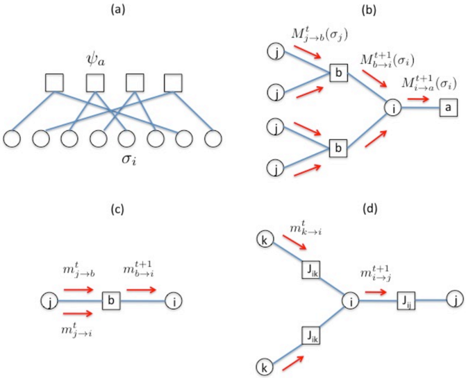<details> <summary>Image 7 Details</summary>  ### Visual Description ## Diagram: Factor Graph and Message Passing ### Overview The image presents four diagrams (a, b, c, d) illustrating factor graphs and message passing algorithms. Diagram (a) shows a factor graph with variable nodes and factor nodes. Diagrams (b), (c), and (d) depict message passing between nodes in different configurations. ### Components/Axes * **(a) Factor Graph:** * Variable nodes: Represented by circles, labeled as "σi". There are 6 variable nodes. * Factor nodes: Represented by squares, labeled as "ψa". There are 4 factor nodes. * Edges: Blue lines connecting variable nodes to factor nodes. * **(b) Message Passing (Complex):** * Nodes: Circles labeled "j", "i", and a square labeled "a", and squares labeled "b". * Messages: Red arrows indicating the direction of message passing. * Message labels: "Mjt→b(σj)", "Mb→i(σi)t+1", "Mi→a(σi)t+1". * **(c) Message Passing (Simple):** * Nodes: Circles labeled "j" and "i", and a square labeled "b". * Messages: Red arrows indicating the direction of message passing. * Message labels: "mjt→b", "mjt→i", "mbt→i+1". * **(d) Message Passing (with J nodes):** * Nodes: Circles labeled "k", "i", and "j", and squares labeled "Jik" and "Jij". * Messages: Red arrows indicating the direction of message passing. * Message labels: "mkt→i", "mit→j+1". ### Detailed Analysis or Content Details * **(a) Factor Graph:** The factor graph shows the relationship between variables σi and factors ψa. Each variable node is connected to one or more factor nodes, indicating that the factor depends on those variables. * **(b) Message Passing (Complex):** Messages are passed from variable nodes "j" to factor nodes "b", then from "b" to variable node "i", and finally from "i" to factor node "a". The messages are functions of the variables σj and σi, and they are updated iteratively (indicated by the superscripts t and t+1). * **(c) Message Passing (Simple):** Messages are passed from variable node "j" to factor node "b", and then from "b" to variable node "i". The messages are updated iteratively. * **(d) Message Passing (with J nodes):** Messages are passed from variable nodes "k" to intermediate nodes "Jik", then to variable node "i", and finally to node "Jij" and variable node "j". The messages are updated iteratively. ### Key Observations * The diagrams illustrate different configurations of nodes and message passing schemes. * The messages are updated iteratively, suggesting an iterative algorithm for inference or optimization. * The factor graph provides a graphical representation of the dependencies between variables and factors. ### Interpretation The diagrams depict the core concepts of factor graphs and message passing algorithms, which are widely used in probabilistic inference, machine learning, and signal processing. The factor graph provides a clear representation of the dependencies between variables and factors, while the message passing algorithms provide a way to efficiently compute marginal probabilities or optimize objective functions. The different configurations of nodes and message passing schemes illustrate the flexibility of these techniques in handling various types of problems. The iterative nature of the message passing algorithms suggests that they can converge to a solution after multiple iterations. </details> BP can then be viewed as an iterative dynamical algorithm for computing a marginal 𝑃𝑃 ( 𝜎𝜎 𝑖𝑖 ) by passing messages along the factor graph. In the case of combinatorial optimization, we can focus on the zero temperature 𝛽𝛽→∞ limit. We will first describe the BP algorithm intuitively, and later give justification for it. BP employs two types of messages: one from variables to factors and another from factors to variables. Each message is a probability distribution over a single variable. We denote by 𝑀𝑀 𝑖𝑖→𝑏𝑏 𝑡𝑡 ( 𝜎𝜎 𝑖𝑖 ) the message from variable 𝑗𝑗 to factor 𝑏𝑏 at iteration time 𝑡𝑡 . It can be thought of intuitively as an approximation to the marginal distribution of 𝜎𝜎 𝑖𝑖 induced by all other interactions 𝑎𝑎 ≠ 𝑏𝑏 . Thus 𝑀𝑀 𝑖𝑖→𝑏𝑏 𝑡𝑡 ( 𝜎𝜎 𝑖𝑖 ) models the distribution over 𝜎𝜎 𝑖𝑖 in a cavity system in which interaction 𝑏𝑏 has been removed. Furthermore, we denote by 𝑀𝑀 𝑏𝑏→𝑖𝑖 𝑡𝑡 ( 𝜎𝜎 𝑖𝑖 ) the message from factor 𝑏𝑏 to variable 𝑖𝑖 at iteration time 𝑡𝑡 . Intuitively, we can think of 𝑀𝑀 𝑏𝑏→𝑖𝑖 𝑡𝑡 ( 𝜎𝜎 𝑖𝑖 ) as the distribution on 𝜎𝜎 𝑖𝑖 induced by the direct influence of interaction 𝑏𝑏 . These messages are called beliefs, as they indicate various probabilities that different interactions believe a single variable should assume. The BP equations amount to updating these beliefs to make them self-consistent with each other. For example, the (unnormalized) update equation for messages from factors to variables (see Fig. 7b) takes the form 𝑀𝑀 𝑏𝑏→𝑖𝑖 𝑡𝑡+1 ( 𝜎𝜎 𝑖𝑖 ) = ∑ 𝜓𝜓 𝑏𝑏 ( 𝜎𝜎 𝑏𝑏 ) 𝜎𝜎 𝑏𝑏 / 𝑖𝑖 ∏ 𝑀𝑀 𝑖𝑖→𝑏𝑏 𝑡𝑡 ( 𝜎𝜎 𝑖𝑖 ) 𝑖𝑖 ∈ 𝑏𝑏 / 𝑖𝑖 . Here, 𝑏𝑏 / 𝑖𝑖 denotes the set of all variables in set 𝑏𝑏 with variable 𝑖𝑖 removed. Intuitively, the direct influence 𝑀𝑀 𝑏𝑏→𝑖𝑖 𝑡𝑡+1 ( 𝜎𝜎 𝑖𝑖 ) of interaction 𝑏𝑏 on variable 𝑖𝑖 is computed by integrating out of the factor 𝜓𝜓 𝑏𝑏 ( 𝜎𝜎 𝑏𝑏 ) all variables 𝑗𝑗 participating in interaction 𝑏𝑏 other than 𝑖𝑖 , supplemented by accounting for the effect of all other interactions besides 𝑏𝑏 by the product of beliefs 𝑀𝑀 𝑖𝑖→𝑏𝑏 𝑡𝑡 ( 𝜎𝜎 𝑖𝑖 ) over all variables 𝑗𝑗 ∈ 𝑏𝑏 / 𝑖𝑖 . This product structure essentially encodes an implicit assumption that the variables 𝑗𝑗 ∈ 𝑏𝑏 would be independent of each other if interaction 𝑏𝑏 were removed. This would be exactly true if the factor graph were a tree with no loops. Similarly, the messages from variables to factors are updated via 𝑀𝑀 𝑖𝑖→𝑎𝑎 𝑡𝑡+1 ( 𝜎𝜎 𝑖𝑖 ) = ∏ 𝑀𝑀 𝑏𝑏→𝑖𝑖 𝑡𝑡+1 ( 𝜎𝜎 𝑖𝑖 ) 𝑏𝑏 ∈ 𝑖𝑖 / 𝑎𝑎 (see Fig. 7b). Intuitively, the belief 𝑀𝑀 𝑖𝑖→𝑎𝑎 𝑡𝑡+1 ( 𝜎𝜎 𝑖𝑖 ) on variable 𝑖𝑖 induced by all other interactions besides 𝑎𝑎 is simply the product of the direct influences 𝑀𝑀 𝑏𝑏→𝑖𝑖 𝑡𝑡+1 ( 𝜎𝜎 𝑖𝑖 ) of all interactions 𝑏𝑏 that involve variable 𝑖𝑖 besides interaction 𝑎𝑎 (this set of interactions is denoted by 𝑖𝑖 / 𝑎𝑎 ). Belief propagation involves randomly initializing the messages and repeating these iterations until convergence. If the messages converge, the marginal distribution of any variable can be computed as P( 𝜎𝜎 𝑖𝑖 ) = ∏ 𝑀𝑀 𝑎𝑎→𝑖𝑖 𝑡𝑡 ( 𝜎𝜎 𝑖𝑖 ) 𝑎𝑎 ∈ 𝑖𝑖 . In essence the marginal is the product of all direct influences 𝑀𝑀 𝑎𝑎→𝑖𝑖 𝑡𝑡 ( 𝜎𝜎 𝑖𝑖 ) over all interactions 𝑎𝑎 that contain variable 𝑖𝑖 . For a general factor graph, there is no guarantee that the BP update equations will converge in finite time, and even if they do, there is no guarantee the converged messages will yield accurate marginal distributions. However, if the factor graph is a tree, then it can be proven that the BP update equations do indeed converge, and moreover they converge to the correct marginals. [64] Moreover, even in graphs with loops, the fixed points of the BP update equations were shown to be in one to one correspondence with extrema of a certain Bethe free energy approximation to the true free energy associated with the factor graph distribution. [71] This observation yielded a seminal connection between BP in computer science, and the Bethe approximation in statistical physics. The exactness of BP on tree graphs, as well as the variational connection between BP and Bethe free energy on graphs with loops, motivated the further study of BP updates in sparsely connected random factor graphs in which loops are of size O(log N). In many such settings BP updates converge and yield good approximate marginals. [66] In particular, if correlations between variables 𝑖𝑖 ∈ 𝑎𝑎 adjacent to a factor 𝑎𝑎 are weak upon removal of that factor, then BP is thought to work well. Now specializing to the case of Ising spins in which each variable 𝜎𝜎 = ±1 , every message 𝑀𝑀 ( 𝜎𝜎 ) is a distribution over a single spin, and can be uniquely characterized by a field ℎ via the relation 𝑀𝑀 ( 𝜎𝜎 ) ∝ 𝑒𝑒 𝛽𝛽ℎ or equivalently through the magnetization 𝑚𝑚 = 𝑡𝑡𝑎𝑎𝑛𝑛ℎ ( 𝛽𝛽ℎ ). Thus the BP update equations for the beliefs 𝑀𝑀 𝑖𝑖→𝑏𝑏 𝑡𝑡 ( 𝜎𝜎 𝑖𝑖 ) and 𝑀𝑀 𝑏𝑏→𝑖𝑖 𝑡𝑡 ( 𝜎𝜎 𝑖𝑖 ) can be viewed as a discrete time dynamical system on a collection of real valued fields ℎ𝑖𝑖→𝑏𝑏 𝑡𝑡 and ℎ𝑏𝑏→𝑖𝑖 𝑡𝑡 or equivalent magnetizations 𝑚𝑚 𝑖𝑖→𝑏𝑏 𝑡𝑡 and 𝑚𝑚 𝑏𝑏→𝑖𝑖 𝑡𝑡 . Furthermore, in the case of pairwise interactions, where between any pair of spins there is at most one interaction, we can further simplify the BP equations. For instance, along any directed edge from spin 𝜎𝜎 𝑖𝑖 to spin 𝜎𝜎 𝑖𝑖 passing through an interaction 𝑏𝑏 with coupling constant 𝐽𝐽 𝑖𝑖𝑖𝑖 , BP maintains two messages, parameterized by 𝑚𝑚 𝑖𝑖→𝑏𝑏 𝑡𝑡 and 𝑚𝑚 𝑏𝑏→𝑖𝑖 𝑡𝑡+1 where 𝑚𝑚 𝑏𝑏→𝑖𝑖 𝑡𝑡+1 is solely a function of 𝑚𝑚 𝑖𝑖→𝑏𝑏 𝑡𝑡 , 𝐽𝐽 𝑖𝑖𝑖𝑖 , and 𝛽𝛽 (Fig. 7(c)). Thus we can write the BP update equations for Ising systems solely in terms of one of the messages, which we rename to be 𝑚𝑚 𝑖𝑖→𝑖𝑖 𝑡𝑡 ≡ 𝑚𝑚𝑖𝑖→𝑏𝑏 𝑡𝑡 . Thus for each connection in the Ising system, there are now two magnetizations: 𝑚𝑚 𝑖𝑖→𝑖𝑖 𝑡𝑡 and 𝑚𝑚 𝑖𝑖→𝑖𝑖 𝑡𝑡 corresponding to messages flowing along the two directions of the connection. Intuitively, 𝑚𝑚 𝑖𝑖→𝑖𝑖 𝑡𝑡 is the magnetization of spin 𝜎𝜎 𝑖𝑖 in a cavity system where the coupling 𝐽𝐽 𝑖𝑖𝑖𝑖 has been removed. Similarly, 𝑚𝑚 𝑖𝑖→𝑖𝑖 𝑡𝑡 is the magnetization of spin 𝜎𝜎 𝑖𝑖 in the same cavity system with coupling 𝐽𝐽 𝑖𝑖𝑖𝑖 removed. Some algebra reveals [66][68] that the BP equations in terms of the cavity magnetizations 𝑚𝑚 𝑖𝑖→𝑖𝑖 𝑡𝑡 are given by $$m _ { i \rightarrow j } ^ { t + 1 } \, = \, \tanh \left [ \sum _ { k \in i / j } \tanh ^ { - 1 } \{ \tanh \left ( \beta J _ { i k } \right ) m _ { k \rightarrow i } ^ { t } \} \right ] .$$ Here the sum over 𝑘𝑘 ∈ 𝑖𝑖 / 𝑗𝑗 denotes a sum over all neighbors of spin 𝑖𝑖 other than spin 𝑗𝑗 . See Fig. 7d for a visualization of the flow of messages underlying Eq. 3. These BP equations maintain two magnetizations associated with each connection in the Ising system, corresponding to the two directions of flow across each edge. The messages are initialized randomly and updated according to equation (3), with the magnetizations thus flowing bi-directionally through the Ising network, hopefully converging to a set of fixed point magnetizations. The marginal of a spin 𝜎𝜎 𝑖𝑖 at iteration 𝑡𝑡 is then given by the magnetization 𝑚𝑚 𝑖𝑖 𝑡𝑡 = tanh �∑ tanh -1 � tanh ( 𝛽𝛽𝐽𝐽 𝑖𝑖𝑖𝑖 ) 𝑚𝑚 𝑖𝑖→𝑖𝑖 𝑡𝑡 � 𝑖𝑖 ∈ 𝑖𝑖 � . While this dynamics promotes the spin variables to analog variables, like the classical CIM dynamics in Eq. 1, it also bears three salient differences from the CIM dynamics: it operates in discrete time, maintains two analog variables per edge, rather than one analog variable per spin, and uses a different nonlinearity. Of course, the specialized BP dynamics are expected to work well specifically for classes of sparsely connected tree-like Ising systems in which removing an interaction 𝐽𝐽 𝑖𝑖𝑖𝑖 from the system makes the spins 𝜎𝜎 𝑖𝑖 and 𝜎𝜎 𝑖𝑖 approximately independent, but are not guaranteed to yield accurate marginals in more general settings. The BP equations for Ising systems can also be used to derive the famous TAP equations [72] for the Sherrington Kirkpatrick (SK) model, [35] where each coupling constant 𝐽𝐽 𝑖𝑖𝑖𝑖 is chosen i.i.d from a zero mean Gaussian distribution with variance 1/ 𝑁𝑁 . Because the couplings are now 𝑂𝑂 (1/ √𝑁𝑁 ) , we can Taylor expand Eq. 3 to obtain 𝑚𝑚 𝑖𝑖→𝑖𝑖 𝑡𝑡+1 = tanh �∑ 𝛽𝛽𝐽𝐽 𝑖𝑖𝑖𝑖 𝑚𝑚 𝑖𝑖→𝑖𝑖 𝑡𝑡 𝑖𝑖 ∈ 𝑖𝑖 / 𝑖𝑖 � . Now this update equation is written in terms of cavity magnetizations 𝑚𝑚 𝑖𝑖→𝑖𝑖 𝑡𝑡+1 in a system in which a single coupling 𝐽𝐽 𝑖𝑖𝑖𝑖 is removed. Because the SK model connectivity is dense with each individual coupling 𝑂𝑂 (1/ √𝑁𝑁 ) , each cavity magnetization 𝑚𝑚 𝑖𝑖→𝑖𝑖 𝑡𝑡+1 with 𝐽𝐽 𝑖𝑖𝑖𝑖 removed, is close to the actual magnetization 𝑚𝑚 𝑖𝑖 𝑡𝑡+1 when 𝐽𝐽 𝑖𝑖𝑖𝑖 is present. By Taylor expanding in the small difference between 𝑚𝑚 𝑖𝑖→𝑖𝑖 𝑡𝑡+1 and 𝑚𝑚 𝑖𝑖 𝑡𝑡+1 , one can write the BP update equations for the case of dense mean field connectivity solely in terms of the variables 𝑚𝑚 𝑖𝑖 𝑡𝑡+1 (see [68] for a derivation of the TAP equations from this BP perspective): $$m _ { i } ^ { t + 1 } \, = \, \tanh \left [ \sum _ { j } \beta J _ { i j } \, m _ { j } ^ { t } \, - \, \beta ^ { 2 } \, m _ { i } ^ { t - 2 } \, \sum _ { j } J _ { i j } ^ { 2 } \{ 1 - ( m _ { j } ^ { t - 1 } ) ^ { 2 } \} \right ]$$ This achieves a dramatic simplification in the dynamics of Eq. 3 from tracking 2 𝑁𝑁 2 variables to only tracking N variables, and as such is more similar to the CIM dynamics in Eq. 1. Again there are still several differences: the dynamics in Eq. 4 is discrete time, uses a different nonlinearity, and has an interesting structured history dependence extending over two time steps. Remarkably, although BP was derived with the setting of sparse random graphs in mind, the particular form of the approximate BP equations for the dense mean field SK model can be proven to converge to the correct magnetizations as long as the SK model is outside of the spin glass phase. [73] So far, we have seen a set of analog approaches to solving Ising systems in specialized cases (sparse random and dense mean field connectivities). However, these local update rules do not work well when such connectivities exhibit spin glass behavior. It is thought that the key impediment to local algorithms working well in the spin glass regime is the existence of multiple minima in the free energy landscape over spin configurations. [66] This multiplicity yields a high reactivity of the spin system to the addition or flip of a single spin. For example, if a configuration is within a valley with low free energy, and one forces a single spin flip, this external force might slightly raise the energy of the current valley and lower the energy of another valley that is far away in spin configuration space but nearby in energy levels, thereby making these distant spin configurations preferable from an optimization perspective. In such a highly reactive situation, flipping one spin at a time will not enable one to jump from valleys that were optimal (lower energy) before the spin flip, to a far away valley that is now more optimal (even lower energy) after the spin flip. This physical picture of multiple valleys that are well separated in spin configuration space, but whose energies are near each other, and can therefore reshuffle their energy orders upon the flips of individual spins, motivated the invention of alternative algorithms that extend belief propagation to survey propagation. The key idea, in the context of an Ising system, is that the magnetizations 𝑚𝑚𝑖𝑖→𝑖𝑖 of BP now correspond to the magnetizations of spin configurations in a single free energy valley (still in a cavity system with the coupling 𝐽𝐽 𝑖𝑖𝑖𝑖 removed). SP goes beyond this to keep track of the distribution of BP messages across all the free energy valleys. We denote this distribution at iteration 𝑡𝑡 by 𝑃𝑃 𝑡𝑡 ( 𝑚𝑚𝑖𝑖→𝑖𝑖 ) . The distribution over BP beliefs is called a survey . SP propagates these surveys, or distributions over the BP messages across different valleys, taking into account changes in the free energy of the various valleys before and after the addition of a coupling 𝐽𝐽 𝑖𝑖𝑖𝑖 . This more nonlocal SP algorithm can find solutions to hard constraint satisfaction problems in situations where the local BP algorithm fails. [65] Furthermore, recent work going beyond SP, but specialized to the SK model, yields message passing equations that can probably find near ground state spin configurations of the SK model (under certain widely believed assumptions about the geometry of the SK model's free energy landscape) but with a time that grows with the energy gap between the found solution and the ground state. [36] Interestingly, the promotion of the analog magnetizations 𝑚𝑚 𝑖𝑖→𝑖𝑖 𝑡𝑡+1 of BP to distributions 𝑃𝑃 𝑡𝑡 ( 𝑚𝑚𝑖𝑖→𝑖𝑖 ) over these magnetizations is qualitatively reminiscent of the promotion of the classical analog variables of the CIM to quantum wavefunctions over these variables. However this is merely an analogy to be used as a potential inspiration for both understanding and augmenting current quantum CIM dynamics. Moreover, the SP picture cannot account for quantum correlations. Overall, much further theoretical and empirical work needs to be done in obtaining a quantitative understanding the behavior of the CIM in the quantum regime, and the behavior of SP for diverse combinatorial Ising spin systems beyond the SK model, as well as potential relations between the two approaches. An intriguing possibility is that the quantum CIM dynamics enables a nonlocal parallel search over multiple free energy valleys in a manner that may be more powerful than the SP dynamics due to the quantum nature of the CIM. ## Future Outlook While current MFB-CIM hardware implementations would not seem capable of sustaining even limited transient entanglement because of their continual projection of each spin-amplitude on each round trip, it is possible that near-term prototypes could probe quantum-perturbed CIM dynamics at least in the small𝑁𝑁 regime. A recent analysis [74] of a modified MFB-CIM architecture utilizing entanglement swapping-type measurements shows that it should be possible to populate entangled states (of specific structure determined by the measurement configuration) of the spin-amplitudes, if the round-trip optical losses can be made sufficiently small. This type of setup could be used to enable certain entanglement structures to be created by transient non-local flow of quantum states through phase space, or to create specific entangled initial states for future CIM algorithms that exploit quantum interference in some more directed way. One may speculate that the impact of quantum phenomena could become more pronounced in CIMs with extremely low pump threshold, for which quantum uncertainties could potentially be larger relative to the scale of topological structures in the mean-field (in a quantum-optical sense) phase space in the critical near-threshold regime. Prospects for realizing such low-threshold CIM hardware have recently been boosted by progress towards the construction of optical parametric oscillators using dispersion-engineered nanophotonic lithium niobate waveguides and ultra-fast pump pulses. [75] For methods that rely on the relaxation of a potential function, either a Lyapunov function for dynamical systems or free energy landscape for Monte Carlo simulations, it is generally believed that the exponential increase in the number of local minima is responsible for the difficulty in finding the ground-states. It has been suggested that the presence of an even greater number of critical points may prevent the dynamics from descending rapidly to lower energy states. [76] On the other hand, several recently proposed methods that rely on chaotic dynamics instead of a potential function have achieved good performance in solving hard combinatorial problems, [24][26][62][77][78][79] but the theoretical description of the number of non-trivial traps (limit-cycles or chaotic attractors) in their dynamics is lacking. It is of great interest to extend the study of complexity [76] (that is, the enumeration of local minima and critical points) to the case of chaotic dynamics for identifying the mechanisms that prevent these heuristics to find optimal solutions of combinatorial optimization problems and to derive convergence theorems and guarantees of returning solutions within a bounded ratio of the ground-state energy. The closed-loop CIM has been proposed for improving the mapping of the Ising Hamiltonian when the time-evolution of the system is approximated to the first moment of the in-phase component distribution. Because the CIM has the potential of quantum parallel search [22] if dissipation can be reduced experimentally, it is important to extend the description of the closed-loop CIM to higher moments in order to identify possible computational benefits of squeezed or non-Gaussian states. In order to investigate this possibility but abstain from the difficulties of reaching a sufficiently low dissipation experimentally, the simulation of the CIM in digital hardware is necessary. Another interesting prospect of the CIM is its extension to neuroscience research. One possibility is about merged quantum and neural computing concept. In the quantum theory of CIM, we start with a density operator master equation which takes into account a parametric gain, linear loss, gain saturation (or back conversion loss) and dissipative mutual coupling. By expanding the density operator with either a positive P -function (off-diagonal coherent state expansion), truncated Wigner-function or Husimi-function, we can obtain the quantum mechanical Fokker-Planck equations. Using the Ito rule in the Fokker-Planck equations, we finally derive the c -number stochastic differential equations (c-SDE). [27][28][49] We can use them for numerical simulation of the CIM on classical digital computers. This phase space method of quantum optics can be readily modified for numerical simulation of an open-dissipative classical neural network embedded in thermal reservoirs, where vacuum noise is replaced by thermal noise. We note that an ensemble average over many identical classical neural networks driven by independent thermal noise can reproduce the analog of quantum dynamics (entanglement and quantum discord) across bifurcation point. This scenario suggests a potential 'quantum inspired computation' might be already implemented in the brain. Using the c-SDE of CIM as heuristic algorithm in classical neural network platform, we can perform a virtual quantum parallel search in cyber space. In order to compute the dynamic evolution of the density operator, we have to generate numerous trajectories by c -SDE. This can be done by ensemble averaging or time averaging. However, what we need in the end is only the CIM final state, which is one of degenerate ground states, and in such a case, producing just one trajectory by c-SDE is enough. This is the unique advantage of the CIM approach and provided by the fact that this system starts computation as a quantum analog device and finishes it as a classical digital device. It is an interesting open question if the classical neural network in the brain implements such c-SDE dynamics driven by thermal reservoir noise. One of the important challenges in theoretical neuro-science is to answer how large number of neurons collectively interact to produce a macroscopic and emergent order such as decision making, cognition and consciousness via noise injected from thermal reservoirs and critical phenomena at phase transition point. [80][81][82][83] The quantum theory of the CIM may shed a light on this interesting frontier at physics and neuro-science interface. Above we also reviewed a set of qualitative analogies connecting the CIM approach to combinatorial optimization with other approaches in computer science. In particular, we noted that just as the CIM dynamics involves a promotion of the original binary spin variables to classical analog variables and then quantum wave functions associated with these classical variables, computer science based approaches to combinatorial optimization also involve a promotion of the spin variables to analog variables (cavity magnetizations in BP for sparse random connectivities and magnetizations in TAP for dense mean field connectivities), and then distributions over magnetizations in SP. These analogies form a bridge between two previously separate strands of intellectual inquiry, and the crosspollination of ideas between these strands could yield potential insights in both fields. In particular such cross-pollination may both advance the scientific understanding of and engineering improvements upon CIM dynamics. For example, can convergence proofs of BP or TAP equations for special classes of Ising systems shed light on CIM dynamics in these same systems? Can differences between BP, TAP or SP dynamics and CIM dynamics suggest the rational design of better hardware modifications to the CIM, and would such modifications yield improved performance in Ising systems where BP, TAP and SP are known to converge? How would such modifications fare in more difficult settings where BP/TAP and even SP do not converge? Can the success of the CIM in problems other than random Ising systems for which BP, TAP and SP are specialized, suggest more general algorithms that work in other classes of Ising systems? Can the success of the CIM motivate other types of annealing schedules to the energy landscape that could serve as improvements on existing BP, TAP or SP algorithms? Overall the parallels and differences between BP, TAP, SP and CIM thus motivate many intriguing directions for future research that are as of yet completely unexplored. Recently, a variety of different experimental platforms have been proposed and demonstrated for the implementation of Ising spin models. [84][85][86][87][88][89][90] It is expected that theoretical and experimental studies of coherent Ising machines mutually motivate and accelerate the advancement of the field synchronously. More generally, we hope this article provides a sense of the rich possibilities for future interdisciplinary research focused around a multifaceted theoretical and experimental approach to combinatorial optimization uniting perspectives from statistics, computer science, statistical physics, and quantum optics, and making contact with diverse topics like dynamical systems theory, chaos, spin glasses, and belief and survey propagation. ## ACKOWLEDGEMENTS The authors wish to thank Z. Toroczkai, R. L. Byer, M. Fejer, B. Lev, A. Safavi-Naeini, A. Marandi, P. McMahon, D. Englund, W. Oliver, E. Rieffel, P. Ronagh, P. Drummond and M. Reid for their useful discussions. ## DATA AVAILABILITY The data that support the finding of this study are available from the correspondi ng author upon reasonable request. ## REFERENCES - [1] S. Kirkpatrick, C. D. Gelatt, and M. P. Vecchi, Science 220 , 671 (1983). - [2] W. Wang, J. Machta, and H. G. Katzgraber, Phys. Rev. E 92 , 013303 (2015). - [3] G. Zaránd, F. Pázmándi, K. F. Pál, and G. T. Zimányi, Phys. Rev. Lett. 89 , 150201 (2002). - [4] E. Farhi, J. Goldstone, S. Gutmann, J. Lapan, A. Lundgren, and D. Preda, Science 292 , 472 (2001). - [5] T. Kadowaki and H. Nishimori, Phys. Rev. E 58 , 5355 (1998). - [6] T. Wang and J. Roychowdhury, arXiv:1709.08102 (2017). - [7] G. Csaba, A. Raychowdhury, S. Datta, and W. Porod, in 2018 IEEE International Symposium on Circuits and Systems (2018) pp. 1-5. - [8] F. Cai, S. Kumar, T. Van Vaerenbergh, R. Liu, C. Li, S. Yu, Q. Xia, J. J. Yang, R. Beausoleil, W. Lu, and J. P. Strachan, arXiv:1903.11194 (2019). - [9] J. J. Hopfield and D. W. Tank, Biol. Cybern. 52 , 141 (1985). - [10] M. Mezard and A. Montanari, Information, physics, and computation (Oxford University Press, 2009). - [11] S. Geman and D. Geman, IEEE Trans. Pattern Anal. Mach. Intell., 721 (1984). - [12] S. Utsunomiya, K. Takata, and Y. Yamamoto, Optics Express 19 , 18091 (2011). - [13] Z. Wang, A. Marandi, K. Wen, R. L. Byer, and Y. Yamamoto, Phys. Rev. A 88 , 063853 (2013). - [14] A. Marandi, Z. Wang, K. Takata, R. L. Byer, and Y. Yamamoto, Nature Photonics 8 , 937 (2014). - [15] T. Inagaki, Y . Haribara, K. Igarashi, T. Sonobe, S. Tamate, et el., Science 354 , 603 (2016). - [16] P. L. McMahon, A. Marandi, Y. Haribara, R. Hamerly, C. Langrock, S. Tamate, T. Inagaki, H. Takesue, S. Utsunomiya, K. Aihara, et al., Science 354 , 614 (2016). - [17] Y. Takeda, S. Tamate, Y. Yamamoto, H. Takesue, T. Inagaki, and S. Utsunomiya, Quantum Science and Technology 3 , 014004 (2017). - [18] M. Nixon, E. Ronen, A. A. Friesem, and N. Davidson, Phys. Rev. Lett. 110 , 184102 (2013). - [19] N. G. Berloff, M. Silva, K. Kalinin, A. Askitopoulos, J. D. Töpfer, P. Cilibrizzi, W. Langbein, and P. G. Lagoudakis, Nature Materials 16 , 1120 (2017). - [20] K. P. Kalinin and N. G. Berloff, New Journal of Physics 20 , 113023 (2018). - [21] T. Leleu, Y. Yamamoto, S. Utsunomiya, and K. Aihara, Phys. Rev. E 95 , 022118 (2017). - [22] Y. Yamamoto, K. Aihara, T. Leleu, K. Kawarabayashi, S. Kako, M. Fejer, K. Inoue, and H. Takesue, npj Quantum Inf. 3 , 49 (2017). - [23] A. Yamamura, K. Aihara, and Y. Yamamoto, Phys. Rev. A 96 , 053834 (2017). - [24] H. Goto, K. Tatsumura, and A. R. Dixon, Science advances 5 , eaav2372 (2019). - [25] L. K. Grover, Phys. Rev. Lett. 79 , 325 (1997). - [26] T. Leleu, Y. Yamamoto, P. L. McMahon, and K. Aihara, Phys. Rev. Lett. 122 , 040607 (2019). - [27] K. Takata, A. Marandi, and Y . Yamamoto, Phys. Rev. A 92 , 043821 (2015). - [28] D. Maruo, S. Utsunomiya, and Y. Yamamoto, Phys. Scr. 91 , 083010 (2016). - [29] Y. Inui and Y. Yamamoto, arXiv:1905.12348 (2019) - [30] R. Hamerly, T. Inagaki, P. L. McMahon, D. Venturelli, A. Marandi, T. Onodera, E. Ng, C. Langrock, K. Inaba, T. Honjo et al., Science advances 5 , eaau0823 (May 2019). - [31] N. Tezak and H. Mabuchi, EPJ Quantum Technology 2 , 10 (2015). - [32] H. Goto, J. Phys. Soc. Jpn. 88 , 061015 (2019). - [33] M. Stern, H. Sompolinsky, and L. F. Abbott, Phys. Rev. E 90 , 062710 (2014). - [34] Y. N. Dauphin, R. Pascanu, C. Gulcehre, K. Cho, S. Ganguli, and Y . Bengio, in Advances in Neural Information Processing Systems 27 (2014). - [35] D. Sherrington and S. Kirkpatrick, Phys. Rev. Lett. 35 , 1792 (1975). - [36] A. Montanari, Symposium on Foundations of Computer Science (FOCS), 1417 (2019). - [37] A. Yamamura and H. Mabuchi, in preparation. - [38] D. Wennberg, S. Ganguli and H. Mabuchi, in preparation. - [39] A. J. Bray and D. S. Dean, Phys. Rev. Lett. 98 , 150201 (2007). - [40] M. Di Ventra, F. L. Traversa, and I. V . Ovchinnikov, Ann. Phys. (Berlin) 529 , 1700123 (2017). - [41] J. Kempe, Contemporary Physics 44 , 307 (2003). - [42] S. Kako, T. Leleu, Y . Inui, F. Khoyratee, and Y . Yamamoto, Advanced Quantum Technologies (2020). - [43] L-M. Duan, G. Giedke, J. I. Cirac, and P. Zoller, Phys. Rev. Lett. 84 , 2722 (2000). - [44] G. Adesso and A. Datta, Phys. Rev. Lett. 105 , 030501 (2001). - [45] V. B. Braginsky, F. Y . Khalili, and K. S. Thorne, Quantum Measurement (Cambridge University Press, 1992). - [46] Y. Inui and Y. Yamamoto, in preparation. - [47] H. Carmichael, S. Singh, R. Vyas, and P. Rice, Phys. Rev. A 39 , 1200 (1989). - [48] H. M. Wiseman and G. J. Milburn, Phys. Rev. A 47 , 642 (1993). - [49] P. Drummond, K. McNeil, and D. Walls, Journal of Modern Optics 28 , 211 (1981). - [50] S. D. Bartlett, B. C. Sanders, S. L. Braunstein, and K. Nemoto, Phys. Rev. Lett. 88 , 097904 (2002). - [51] J. J. Hopfield and D. W. Tank, Biol. Cybern. 52 , 141 (1985). - [52] H. Sompolinsky and A. Zippelius, Phys. Rev. Lett. 47 , 359 (1981). - [53] D. J. Thouless, P. W. Anderson, and R. G. Palmer, Philosophical Magazine 35 , 593 (1977). - [54] F. Tanaka and S. Edwards, Journal of Physics F: Metal Physics 10 , 2769 (1980). - [55] G. Bilbro, R. Mann, T. K. Miller, W. E. Snyder, D. E. van den Bout, and M. White, in Advances in Neural Information Processing Systems 1 (1988), pp. 91-98. - [56] E. Farhi, J. Goldstone, S. Gutmann, and M. Sipser, arXiv preprint quant-ph/0001106 (2000). - [57] V. Granville, M. Krivanek, and J.-P. Rasson, IEEE Transactions on Pattern Analysis and Machine Intelligence 16 , 652 (1994). - [58] D. Pierangeli, G. Marcucci, D. Brunner, and C. Conti, arXiv:2004.02208 (2020). - [59] S. Geman, and C. R. Hwang, SIAM Journal on Control and Optimization 24 , 1031 (1986). - [60] I. Gershenzon, G. Arwas, S. Gadasi, C. Tradonsky, A. Friesem, O. Raz, and N. Davidson, arXiv:2003.14312 (2020). - [61] K. P. Kalini and N. G. Berloff, Scientific Reports 8 , 17791 (2018). - [62] S. Kumar, J. P. Strachan, and R. S. Williams, Nature 548 , 318 (2017). - [63] U. Benlic, and J.-K. Hao, Eng. Appl. Artif. Intell. 26 , 1162 (2013). - [64] J. Pearl, 'Probabilistic reasoning in intelligent systems: networks of plausible inference,' Morgan Kaufmann Pub. (1988). - [65] A. Braunstein and M. Mézard, and R. Zecchina, Random Struct. Algorithms 27 , 201 (2005), - [66] M. Mézard, and A. Montanari, 'I nformation, physics, and computation,' Oxford University Press, USA (2009). - [67] M. Advani, S. Lahiri, and S. Ganguli, J. Stat. Mech: Theory Exp. 2013 , 030134 (2013). - [68] L. Zdeborová and F. Krzakala, Advances in Physics 65 , 453 (2016). - [69] M. Advani and S. Ganguli, Phys. Rev. X 6 , 031034 (2016). - [70] Y. Bahri, J. Kadmon, J. Pennington, S. S. Schoenholz, J. Sohl-Dickstein, and S. Ganguli, Annual Review of Condensed Matter Physics 11 , 501 (2020), - [71] J. S. Yedidia, W. T. Freeman, and Y. Weiss, IEEE Trans. Inf. Theory 51 , 2282 (2005). - [72] D. J. Thouless, P. W. Anderson, and R. G. Palmer, Philosophical Magazine 35 , 593 (1977). - [73] E. Bolthausen, Communications in Mathematical Physics 325 , 333 (2014) - [74] R. Yanagimoto, P. L. McMahon, E. Ng, T. Onodera and H. Mabuchi, arXiv:1906.04902. - [75] T. Onodera, E. Ng, N. Lorch, A. Yamamura, R. Hamerly, P. L. McMahon, A. Marandi, and H. Mabuchi, arxiv:1811.10583. - [76] G. Biroli, Journal of Physics A: Mathematical and General 32 , 8365 (1999). - [77] M. Ercsey-Ravasz, and Z. Toroczkai, Nature Physics, 7 , 966 (2011). - [78] M. Ercsey-Ravasz and Z. Toroczkai, Sci. Rep. 2 , 725 (2012). - [79] B. Molnár, F. Molnár, M. Varga, Z. Toroczkai, and M. Ercsey-Ravasz, Nature Commun. 9 , 4864 (2018). - [80] A. Levina, J. M. Herrman, and T. Geisel, Nature Physics 3 , 857 (2007). - [81] D. R. Chialvo, Nature Physics 6 , 744 (2010). - [82] T. Mora and W. Bialek, J. Statistical Physics 144 , 268 (2011). - [83] J. Beggs, Phys. Rev. Lett. (Editorial) 114 , 220001 (2015). - [84] M. Babaeian, D. T. Nguyen, V. Demir, M. Akbulut, P-A Blanche, Y. Kaneda, S. Guha, M. A. Neifeld, and N. Peyghambarian, Nat. Commun. 10, 3516 (2019). - [85] D. Pierangeli, G. Marcucci, and C. Conti, Phys. Rev. Lett. 122, 213902 (2019). - [86] F. Böhm, G. Verschaffelt, and G. Van der Sande, Nat. Commun. 10, 3538 (2019). - [87] Y. Okawachi, M. Yu, J. K. Jang, X. Ji, Y . Zhao, B. Y , Kim, M. Lipson, and A. L. Gaeta, arXiv:2003.11583 (2020). - [88] F. Cai, S. Kumar, T. Van Vaerenbergh, X. Sheng, R. Liu, C. Li, Z. Liu, M. Foltin, S. Yu, Q. Xia, et al., Nat. Electron. 3, 409 (2020). - [89] C. Roques-Carmes, Y. Shen, C. Zanoci, M. Prabhu, F. Atieh, L. Jing, T. Dubček, C. Mao, M. R. Johnson, V. Čeperić, et al., Nat. Commun. 11, 249 (2020). - [90] M. Prabhu, C. Roques-Carmes, Y. Shen, N. Harris, L. Jing, J. Carolan, R. Hamerly, T. Baehr-Jones, M. Hochberg, V. Čeperić, et al., Optica 7, 551 (2020).