## Streaming Computations with Region-Based State on SIMD Architectures
Stephen Timcheck and Jeremy Buhler
Washington University in St. Louis One Brookings Dr., St. Louis, MO 63130, USA { stimcheck,jbuhler } @wustl.edu
Abstract. Streaming computations on massive data sets are an attractive candidate for parallelization, particularly when they exhibit independence (and hence data parallelism) between items in the stream. However, some streaming computations are stateful, which disrupts independence and can limit parallelism. In this work, we consider how to extract data parallelism from streaming computations with a common, limited form of statefulness. The stream is assumed to be divided into variably-sized regions , and items in the same region are processed in a common context of state. In general, the computation to be performed on a stream is also irregular , with each item potentially undergoing different, data-dependent processing.
This work describes mechanisms to implement such computations efficiently on a SIMD-parallel architecture such as a GPU. We first develop a low-level protocol by which a data stream can be augmented with control signals that are delivered to each stage of a computation at precise points in the stream. We then describe an abstraction, enumeration and aggregation , by which an application developer can specify the behavior of a streaming application with region-based state. Finally, we study an implementation of our ideas as part of the MERCATOR system [5] for irregular streaming computations on GPUs, investigating how the frequency of region boundaries in a stream impacts SIMD occupancy and hence application performance. 1
Keywords: signal · control message · SIMD · irregular · streaming
## 1 Introduction
Streaming computations are integral to high-impact applications such as biological sequence analysis [1], astrophysics [13], and decision cascades in machine learning [14]. These computations operate on a long stream of data items, each of which must be processed through a pipeline of computational stages. When items can be processed independently and identically, extracting data parallelism is straightforward, particularly on SIMD-parallel architectures such as GPUs.
1 Presented at 13th Int'l Wkshp. on Programmability and Architectures for Heterogeneous Multicores, Bologna, Italy, Jan 2020 . Copyright c © 2020 by Stephen Timcheck and Jeremy Buhler. All rights reserved.
A greater challenge lies in supporting streaming computations whose behavior deviates from the above ideal. Deviations can occur in two ways. First, items may not be processed identically; in particular, some stages of the pipeline may produce a variable, data-dependent amount of output for each input item. Such computations - which include all the examples cited above as well as applications in, e.g., particle simulation [2] and network packet processing [10] are said to exhibit irregular data flow, which complicates the lock-step execution model of a SIMD-parallel processor. Our prior work on the MERCATOR system [5] describes a way to support such irregular computations on GPUs.
A second deviation, which is the subject of the present work, arises when items in a stream cannot be processed independently; that is, the computation is stateful. To avoid the need for full serialization, we focus on a common scenario in which the input stream is divided into variably-sized regions . Items in one region are processed independently of each other but in a common context. For example, a stream of characters may be grouped into lines or network packets; a stream of edges in a graph may be grouped by their source vertex; or a stream of measurements may be grouped by a common time window or event trigger. Region boundaries are state-change events for the stream - items after a boundary must be processed differently than items before it.
In this work, we investigate mechanisms to support streaming computations with region-based contextual state on SIMD-parallel platforms. Our contributions are threefold. First, we describe a low-level mechanism for precise delivery of control signals between pipeline stages of a streaming application. This mechanism, unlike those described in some prior work (e.g. [12]), supports irregular dataflow. Second, we use this mechanism to construct an abstraction, enumeration and aggregation , that lets application developers express region-based contextual state as part of a streaming application. Finally, we implement our designs in MERCATOR to investigate the performance implications of regional context, exposing a SIMD-specific performance tradeoff between alternate ways of implementing this behavior in applications. The two strategies we examine trade off between SIMD occupancy and representation overhead.
The remainder of this paper is organized as follows. Section 2 describes the application and architectural models in which we formulate our work and considers related work in other streaming models. Section 3 describes our protocol for synchronizing control signals with a data stream. Section 4 describes the developer-facing abstraction of enumeration and aggregation, which we implement in terms of signals. Section 5 investigates the performance of our designs, while Section 6 concludes and considers future work.
## 2 Background and Related Work
## 2.1 Application Model
A streaming application consists of a pipeline of compute nodes connected by fixed-sized data queues . A node consumes a stream of data items from its input
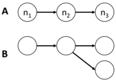
queue and produces a stream of data items (perhaps of a different type) at its output that are queued for processing by the next node downstream in the pipeline. When a node is executed to consume one or more inputs, we say that the node fires . Each input data item consumed by a node causes it to produce zero or more outputs. The number of outputs may vary for each input consumed, up to some node-dependent maximum, and is not known prior to execution. Figure 1a shows a simple application pipeline with three nodes. While we mainly discuss linear pipelines in this work, our contributions also apply to tree-structured topologies like those in Figure 1b.
Fig. 1. (a) Streaming computation pipeline with three compute nodes; (b) Pipeline with a tree topology.
<details>
<summary>Image 1 Details</summary>
### Visual Description
\n
## Diagram: Network Flow Representations
### Overview
The image presents two diagrams, labeled 'A' and 'B', illustrating different network flow structures. Both diagrams use nodes connected by directed arrows to represent the flow. Diagram A shows a linear, sequential flow, while Diagram B depicts a branching flow.
### Components/Axes
The diagrams consist of nodes (circles) and directed edges (arrows).
- **Diagram A:** Contains three nodes labeled n1, n2, and n3. Arrows point from n1 to n2, and from n2 to n3.
- **Diagram B:** Contains four nodes. Arrows point from the first node to the second, from the second to the third, and from the second to the fourth.
### Detailed Analysis or Content Details
**Diagram A:**
- Node n1 is positioned on the left.
- Node n2 is positioned in the center.
- Node n3 is positioned on the right.
- The flow proceeds linearly from n1 -> n2 -> n3.
**Diagram B:**
- The first node is positioned on the left.
- The second node is positioned in the center.
- The third node is positioned on the right.
- The fourth node is positioned below the second node.
- The flow splits from the second node, going to both the third and fourth nodes.
### Key Observations
- Diagram A represents a simple, unidirectional flow through a series of nodes.
- Diagram B represents a flow that diverges, indicating a branching or decision point.
- The diagrams do not contain any numerical data or scales. They are purely structural representations.
### Interpretation
The diagrams likely represent simplified models of processes or systems where elements are connected by directional relationships. Diagram A could represent a sequential process, like a manufacturing line, or a simple chain of events. Diagram B could represent a decision tree, a network with multiple pathways, or a system where a single input can lead to multiple outputs. The absence of quantitative data suggests the diagrams are intended to illustrate the *structure* of the flow rather than its magnitude or rate. The diagrams are conceptual and do not provide specific data points for analysis. They are illustrative examples of network topologies.
</details>
We do not consider DAG-structured topologies because the semantics associated with convergent edges are complex under irregular dataflow, even in the absence of stateful execution [9]. Topologies with cycles have clearer streaming semantics, but in the presence of irregularity, items in the stream can be reordered if they take different numbers of trips around a cycle. For such topologies, Maintaining precisely ordered control boundaries in the stream requires aggressive reordering that is beyond the scope of this work.
An application is provided with an initial stream of inputs to its source node . When the application executes, a global scheduler repeatedly chooses a node with one or more pending inputs to fire. Because of our architectural mapping below, we assume that only one node fires at a time and that a node cannot be preempted while firing. The scheduler continues to select and fire nodes until no node has any inputs remaining.
A signal is a control message generated by a node for consumption by its downstream neighbor. When a node receives a signal it can change its state and may also generate additional signals to the next node downstream. Signals must be delivered precisely with respect to the stream of data items. Formally, suppose we have two successive nodes n 1 and n 2 in a pipeline. If n 1 emits a data item d , followed by a signal s , followed by another data item d ′ , then n 2 must receive s after processing d but before processing d ′ .
## 2.2 Target Architecture and Mapping
Our work targets wide-SIMD multiprocessors. While many general-purpose processors support SIMD instructions, we realize our designs on NVIDIA GPUs due to their robust CUDA tool chain and their popularity as accelerators.
A GPU may be viewed as a collection of SIMD processors sharing a common memory. Each processor has a fixed SIMD width w , which is the number of concurrent SIMD lanes that it can execute 2 . SIMD lanes execute computations
2 We treat the CUDA block size as the effective SIMD width, ignoring CUDA's virtualization of an underlying, smaller width (the warp size).
in lock-step; hence, divergent behavior such as nonuniform branches, or lack of inputs to some SIMD lanes, causes some lanes to sit idle while others execute.
Mapping a streaming computational pipeline onto a GPU entails moving the input stream from the host system to the GPU's memory, executing a GPU kernel to process the data through the pipeline, and finally transferring the output stream back to the host. Our work focuses on efficient processing on the GPU, rather than the orthogonal task of host/GPU data transfer.
GPU runtimes offer little support for interprocessor synchronization other than via control transfer back to the host. To avoid excessive host-device control overhead, we therefore instantiate the pipeline separately on each processor of the GPU, then let all processors' pipelines compete to consume data from a common input stream. This approach requires atomic operations but no locking. The GPU kernel does not return control to the host until the entire stream is consumed. Each processor on the GPU independently implements the sequential, non-preemptively scheduled computation described above. However, a node now consumes not a single input per firing but rather a variably-sized ensemble of inputs, up to the processor's SIMD width, which are processed in parallel.
Our performance goal is to maximize throughput, or equivalently to minimize time for the GPU to process an entire input stream. A secondary goal that promotes high throughput is to maximize SIMD occupancy , the fraction of SIMD lanes doing useful work at any step of the computation. In particular, we want the sizes of ensembles presented to each node to achieve the full SIMD width. However, we will show that region-based state can be in tension with the goal of maximizing SIMD occupancy, creating a challenge for performance optimization.
## 2.3 Related work
Several systems and languages have been developed to express streaming dataflow computations. One of the most influential such systems is StreamIt [11], which implements the synchronous data flow (SDF) abstraction [8]. StreamIt assumes a fixed number of outputs per input to a compute node. This assumption allows StreamIt to offer a powerful abstraction, teleport messaging [12], in which signals can flow both forward and backward in a pipeline. StreamIt can also schedule a signal to be delivered to an arbitrary destination node at some precise future time, rather than forcing the signal to flow through the pipeline.
Many capabilities of teleport messaging rely on the underlying SDF model. In contrast, our model does not assume a fixed number of outputs per input and so requires a different design to ensure precise signaling. Our work therefore extends precise signaling capabilities from regular to irregular streaming applications. Like StreamIt, we choose to send signals 'out of band,' in our case via parallel control edges, rather than attempt to enqueue them together with data items.
Other streaming systems, such as Ptolemy [6] and Auto-Pipe [4], support a variety of dataflow semantics, including multiple, differently-typed dataflow edges between a pair of nodes. This support is in principle sufficient to implement a control channel for signals. However, except in restricted cases like SDF, the
systems do not specify how multiple channels between the same two nodes are synchronized and so do not by themselves support precise signaling.
Our work is influenced by a control messaging protocol developed by Li et al. [9]. That work, however, incurs additional complexity to support asynchronous streaming dataflow and to impose well-defined semantics on convergent dataflow edges in an DAG-structured irregular application. We preserve their idea of a credit protocol for synchronizing data and control streams but realize this idea in a way that is efficient for our target model and architecture.
The idea of processing part of a stream of items in a common context is similar to facilities present in Apache Spark [16]. Spark streams consist of a sequence of RDDs [15], which are discrete data sets, processed as a unit, that may contain multiple elements. Our abstraction supports some operations semantically similar to Spark's but realizes them in the context of a single wide-SIMD processor rather than the multicore and distributed systems that Spark targets.
Other frameworks supporting streaming-like behavior, such as CnC-CUDA [7], utilize an 'in-band' approach with control collections that mix control and data into a single stream. Control collections are analogous to our regions of items with a common context. Their implementation requires a tag for each item to track the region associated with it. In contrast, our implementation keeps region boundaries synchronized with the data stream without the need for tagging. We compare these two approaches in Section 5.
## 3 A Mechanism for Precise Signaling
In this section, we describe how to synchronize data and control signals between two successive nodes in a streaming pipeline. The mechanism bears some similarities to control flow in networking. We state the correctness properties of our design but relegate their proofs to the appendix.
## 3.1 Credit Protocol for Synchronizing Signals
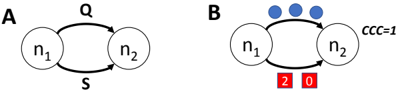
Let n 1 and n 2 be successive nodes in a pipeline, connected by data queue Q . We add a separate, finite-sized signal queue S between the nodes, as in Figure 2a. Data items are moved from n 1 to n 2 on Q , while signals are moved on S .
We must ensure that, although data and signals move on separate queues, their movement is synchronized so as to ensure precise signal delivery. For this purpose, we introduce a credit protocol between n 1 and n 2 . Each signal created by n 1 is assigned an non-negative integer amount of credit , which is transmitted along with the signal on S . Credit records a number of data items that n 2 must process before it can receive the signal.
When n 1 emits a signal s , it uses two rules to set the credit associated with s . (1) If no signal is currently queued on S , then s gets an amount of credit equal to the number of data items queued on Q . (2) If one or more signals are queued on S , let s ′ be the signal at the tail of S . Then s gets an amount of credit equal to the number of data items emitted by n 1 since s ′ was enqueued. Node
n 1 maintains a counter of emitted data items, which is reset each time it emits a signal, that is used to implement the second rule.
The downstream node n 2 maintains a current credit counter , initially set to 0, that tracks the number of items that can safely be consumed before processing the next signal. Node n 2 uses the following two rules to determine whether to process data or a signal when it fires. (1) If no signal is queued on S , n 2 may freely consume any available data items on Q without regard to the counter. Otherwise (i.e., a signal is queued on S ), (2a) if the current credit counter is non-zero, n 2 may consume only a number of data items less than or equal to the value of this counter, which is decremented once for each data item consumed. (2b) If instead the current credit counter is 0, let s be the signal at the head of queue S . If s carries more than 0 credit, that credit is removed from s and added to the current credit counter. Otherwise, n 2 consumes s .
Figure 2b illustrates how the credit carried in the signals and in the receiving node's credit counter synchronizes the two queues.
Lemma 1. A signal s emitted by n 1 is received by n 2 precisely when n 2 has consumed all data items emitted by n 1 prior to s .
## 3.2 Scheduling Applications with Signals
A firing of a node n proceeds in two phases: a data phase and a signal phase . In the data phase, n consumes as many queued data items as it can. The number of items consumed is limited to the minimum of three values: the number of queued items, the amount of space in n 's downstream queue, and (if a signal is pending for n ) the value of n 's current credit counter. Once n can consume no more data, if its current credit counter is 0, it enters the signal phase, in which it consumes as many queued signals as it can. Signal processing ends when no queued signals remain, or when n 's current credit counter becomes > 0 (and hence data must be consumed prior to the next queued signal).
A node is fireable if it has either data or a signal pending, and if there is sufficient space in its output queue to hold any outputs from the firing. The maximum number of output data items per input item is known a priori for each node, so the scheduler can determine whether at least one data item can
<details>
<summary>Image 2 Details</summary>
### Visual Description
\n
## Diagram: State Transition Diagram
### Overview
The image presents two state transition diagrams, labeled A and B, depicting relationships between two states, n1 and n2. Diagram A shows a simple bidirectional transition, while Diagram B includes additional elements representing a constraint and numerical values associated with the transitions.
### Components/Axes
* **Diagram A:**
* States: n1, n2 (represented as circles)
* Transitions: Bidirectional arrows connecting n1 and n2.
* Labels: "Q" above the transition from n1 to n2, "S" below the transition from n2 to n1.
* **Diagram B:**
* States: n1, n2 (represented as circles)
* Transitions: Bidirectional arrows connecting n1 and n2.
* Constraint: Three blue circles positioned above the transition arrows.
* Numerical Values: "2" below n1 and "0" below n2, enclosed in red boxes.
* Label: "CCC=1" to the right of n2.
### Detailed Analysis or Content Details
* **Diagram A:** The diagram shows a simple bidirectional relationship between states n1 and n2. The transition from n1 to n2 is labeled "Q", and the transition from n2 to n1 is labeled "S". There are no numerical values or constraints indicated.
* **Diagram B:** This diagram also shows a bidirectional relationship between n1 and n2. However, it includes a constraint represented by three blue circles above the arrows. The state n1 is associated with the value "2", and n2 is associated with the value "0". The label "CCC=1" suggests a constraint or condition related to the system.
### Key Observations
* Diagram B introduces numerical values and a constraint not present in Diagram A.
* The numerical values "2" and "0" are directly associated with states n1 and n2, respectively.
* The constraint "CCC=1" might represent a condition that must be met for the transitions to occur or a property of the system.
* The blue circles above the arrows in Diagram B could represent a condition or a set of possible transitions.
### Interpretation
These diagrams likely represent a simplified model of a system with two states. Diagram A shows a basic interaction, while Diagram B adds complexity with constraints and numerical values. The values "2" and "0" could represent quantities, probabilities, or other relevant parameters. The constraint "CCC=1" suggests a specific condition that governs the system's behavior. The blue circles could represent possible states or events that influence the transitions between n1 and n2.
Without further context, it's difficult to determine the exact meaning of these diagrams. However, they likely represent a system where the transition between states is influenced by a constraint and is associated with specific numerical values. The diagrams could be used to model a chemical reaction, a biological process, or a computational system. The "Q" and "S" labels could represent specific actions or events that trigger the transitions.
</details>
S
Fig. 2. (a) Two nodes with data and signal queues Q and S between them; (b) A possible state of the signal protocol, showing the credit associated with each signal (lower edge) and the current credit counter (right). n 2 may consume one data item from Q before the first signal, then another two before the second signal.
be consumed given the available space on n 's downstream data queue. The maximum number of signals emitted per data item or signal input is also known a priori , so a similar determination can be made given n 's downstream signal queue. The scheduler repeatedly chooses some fireable node and fires it until no node has queued data or signals remaining.
Lemma 2. Under the given firing/scheduling policy, an application pipeline always finishes execution in finite time and so cannot deadlock.
## 3.3 SIMD Extensions
The above description assumes that nodes process input data items one at a time. However, on a SIMD-parallel processor, a node may process an ensemble of multiple items at once. Because a signal updates the state of the receiving node, we must ensure that items appearing before and after a signal in the stream are not processed in the same input ensemble . Hence, if a signal is queued for a node, the system must limit the size of the node's input ensemble to the value of its current credit counter. This requirement may adversely impact SIMD occupancy if signals occur frequently; we study its impact in Section 5.
## 4 Regional Context via Enumeration and Aggregation
We now describe a developer-facing abstraction, enumeration and aggregation , that allows application developers to describe streaming computations in which regions of a stream must be processed in a common context. We have implemented this abstraction as an extension to our MERCATOR system, building on the work of the previous section.
Our abstraction assumes that regions of a stream with a common context are represented as composite objects , similar to the RDDs of Apache Spark [16]. The actual input provided to the application is a stream of such objects. Each object may contain zero or more elements of a common data type. For example, an object could be a line of text whose elements are characters, or a vertex whose elements are its adjacent edges, or a list whose elements are numbers. Objects may contain different numbers of elements.
At a given point in the application's pipeline, the developer may choose to 'open' the stream of composite objects to create a stream of all their elements. We call this opening process enumeration of the objects. The enumerated element stream becomes the input to the next node in the pipeline. In this and subsequent nodes, the developer may access the parent object that gave rise to an input item to obtain context needed for its processing.
The opposite of enumeration is aggregation , which 'closes' the context associated with a parent object. The developer may choose to emit a stream of results derived from individual elements, stripped of their parent context, or to aggregate values computed from the elements of each parent object (e.g. by summing them) and emit a single result per parent. Either way, the stream of results continues down the pipeline.
## 4.1 Developer Interface
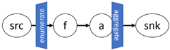
To make these ideas concrete, consider the simple application whose topology is sketched in Figure 3. A stream of objects of type Blob , each containing a collection of numbers, flows from the source node. The Blobs' elements are enumerated, and node f does some computation on each number in the element stream, producing a (possibly shorter) output stream of numbers. These results are passed to node a , which sums the results from each Blob and sends a stream of per-Blob sums to a sink node.
Fig. 3. A pipeline with enumeration and aggregation. The computation enumerates composite objects drawn from an input source, acts on their elements with a filtering node f , aggregates the filtered values in an accumulator node a , and writes the accumulated value from each object to an output sink.
<details>
<summary>Image 3 Details</summary>
### Visual Description
\n
## Diagram: Data Flow
### Overview
The image depicts a simple data flow diagram with four components connected by directed edges. The diagram illustrates a sequential process where data flows from a source ("src") through intermediate stages ("f" and "a") to a sink ("snk"). Two "enumerate" operations are applied between the components.
### Components/Axes
The diagram consists of the following components:
* **src:** Represents the data source.
* **f:** An intermediate processing stage.
* **a:** Another intermediate processing stage.
* **snk:** Represents the data sink or destination.
* **enumerate:** A processing operation applied between "src" and "f", and between "f" and "a". The text "enumerate" is vertically oriented and placed alongside the connecting arrows.
### Detailed Analysis or Content Details
The diagram shows a linear data flow:
1. Data originates at "src".
2. An "enumerate" operation is applied to the data as it flows from "src" to "f".
3. The data is processed by "f".
4. Another "enumerate" operation is applied to the data as it flows from "f" to "a".
5. The data is processed by "a".
6. The data reaches the final destination, "snk".
The arrows indicate the direction of data flow. The "enumerate" operations are visually represented as blue rectangular blocks positioned perpendicular to the data flow arrows.
### Key Observations
The diagram is very simple and does not contain any numerical data or complex relationships. The primary focus is on the sequential flow of data and the application of the "enumerate" operation at two points in the process.
### Interpretation
This diagram likely represents a simplified data pipeline or processing workflow. The "enumerate" operation suggests that the data is being processed in a sequence or indexed in some way. The diagram could be a high-level representation of a data transformation process, a stream processing pipeline, or a similar data-centric operation. The lack of detail suggests it's an abstract illustration of a concept rather than a specific implementation. Without further context, it's difficult to determine the exact nature of the data or the purpose of the "enumerate" operation.
</details>
The listing of Figure 4 specifies the application's topology. For each node, we specify the types of its input and output streams. The enumerate keyword at the input to node f indicates that Blobs are to be enumerated starting there; subsequent data types in the enumeration region of the pipeline are labeled from Blob , indicating that items are to be processed in the context of their parent Blobs. Aggregation occurs at the output of node a , where the aggregate keyword indicates that a produces (up to) one double value per parent object rather than per element.
Figure 5 shows code to implement the application. For each node, there is a run() function that processes items in the node's input stream. Output from a node is generated via the push() function; because the application is irregular, not every input might produce an output.
The listing shows several functions specific to enumeration and aggregation. findCount() is called once per parent object to determine how many elements it contains. The begin() and end() functions, which may be defined for each node receiving enumerated inputs, are executed before and after the region of the stream associated with each parent object, respectively. The parent object associated with a node's current input is accessible via getParent() .
Enumeration produces a stream of sequential indices of elements in each parent object. However, the application developer is responsible for providing code to extract the elements from an object. This design allows MERCATOR to remain ignorant of how objects are organized internally.
## 4.2 Implementation
The MERCATOR system takes in an application topology, as shown in Figure 4, and produces stubs for all the functions shown in Figure 5. The user then fills in the function bodies with the actual code of the application.
We note that the code shown is CUDA, not C++ ; hence, the run() functions are actually called not with a single input but with a SIMD ensemble of items in multiple threads, which execute the function body in parallel for each item. (The
```
```
Fig. 4. Application topology specification illustrating enumeration and aggregation.
```
```
Fig. 5. Application code, with stubs generated from topology and developer-supplied function bodies.
accumulation in node a would in practice be implemented atomically or with a SIMD-parallel reduction.) MERCATOR provides the runtime infrastructure needed to transfer data from one node to the next and to schedule nodes.
The signaling mechanism of the previous section is key to enabling enumeration and aggregation. At the point of enumeration, the runtime generates a data stream of element indices together with signals indicating the start and end of each parent object's elements. Downstream nodes intercept these signals in order to update their current parent object and to call the begin() and end() stubs at the right times. Because data before and after a signal is never processed in the same SIMD ensemble, operations on different parent objects' elements always happen in separate calls to a node's run() function, and the result of getParent() is the same for all items in an ensemble.
## 5 Results
We implemented both our precise signaling infrastructure and the enumeration and aggregation abstraction as extensions to our MERCATOR framework and studied their performance on several benchmark computations. All experiments were conducted on an NVIDIA GTX 1080Ti GPU (28 processors), using as many active blocks as could fit on the device and a SIMD width of 128 threads per block. Code was compiled using CUDA v10 under Linux. The abstraction penalty of the new features was verified to be negligible in MERCATOR applications that do not use them.
Cost of Regional Context Abstraction To characterize the performance impact of regional context, we began with two simple benchmark computations. Each benchmark operates on a large array of integers in GPU memory, and each divides this array into a series of regions. The computation enumerates each region, sums its elements, and produces a stream of per-region sums. In the first benchmark, the regions are of uniform size; in the second, the size of each region is chosen uniformly at random between 0 and a specified maximum.
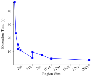
Fig. 6. Execution time vs. region size for sum app with fixed-size regions.
<details>
<summary>Image 4 Details</summary>
### Visual Description
\n
## Line Chart: Execution Time vs. Region Size
### Overview
The image presents a line chart illustrating the relationship between Region Size and Execution Time. The chart shows a decreasing trend in execution time as the region size increases, with a steep initial drop followed by a gradual leveling off.
### Components/Axes
* **X-axis:** Region Size (labeled at the bottom). Scale ranges from approximately 256 to 2048, with markers at 256, 512, 768, 1024, 1280, 1536, 1792, and 2048.
* **Y-axis:** Execution Time (s) (labeled on the left). Scale ranges from approximately 0 to 45, with markers at 0, 10, 20, 30, and 40.
* **Data Series:** A single blue line representing the execution time for different region sizes.
* **No Legend:** There is no explicit legend, but the single line is the sole data representation.
### Detailed Analysis
The blue line starts at approximately 43 seconds at a region size of 256. The line then exhibits a steep downward slope, reaching approximately 24 seconds at a region size of 512. The slope continues to decrease, but at a slower rate, reaching approximately 12 seconds at a region size of 768. The line continues to descend, reaching approximately 8 seconds at a region size of 1024. From 1024 to 1536, the line decreases to approximately 7 seconds. Between 1536 and 1792, the line decreases to approximately 6 seconds. Finally, from 1792 to 2048, the line decreases to approximately 5 seconds.
Here's a more detailed breakdown of approximate data points:
* Region Size: 256, Execution Time: ~43 s
* Region Size: 512, Execution Time: ~24 s
* Region Size: 768, Execution Time: ~8 s
* Region Size: 1024, Execution Time: ~8 s
* Region Size: 1280, Execution Time: ~6 s
* Region Size: 1536, Execution Time: ~7 s
* Region Size: 1792, Execution Time: ~6 s
* Region Size: 2048, Execution Time: ~5 s
### Key Observations
* The most significant reduction in execution time occurs with smaller region sizes (256 to 768).
* As the region size increases beyond 1024, the decrease in execution time becomes marginal.
* The curve appears to be approaching an asymptote, suggesting that further increases in region size will yield diminishing returns in terms of execution time reduction.
### Interpretation
The data suggests that increasing the region size generally improves execution performance, but there's a point of diminishing returns. The initial steep decline indicates that smaller region sizes are significantly less efficient. This could be due to overhead associated with processing smaller regions, such as increased context switching or memory access costs. As the region size grows, these overheads become less significant, leading to a more gradual improvement in execution time. The leveling off of the curve suggests that the benefits of further increasing the region size are minimal, and may even be offset by other factors, such as increased memory usage or cache misses. This information is valuable for optimizing the performance of systems that process data in regions, as it helps determine the optimal region size to balance execution time and resource consumption. The chart implies that a region size of around 1024 or greater provides a good balance between performance and efficiency.
</details>
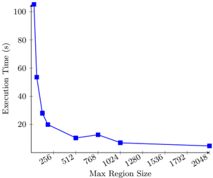
Fig. 7. Execution time vs. max region size for sum app with variable regions.
<details>
<summary>Image 5 Details</summary>
### Visual Description
\n
## Line Chart: Execution Time vs. Max Region Size
### Overview
The image presents a line chart illustrating the relationship between "Max Region Size" and "Execution Time". The chart shows a steep decrease in execution time as the max region size increases, followed by a leveling off. The chart appears to be evaluating the performance of an algorithm or process as a function of the size of the regions it operates on.
### Components/Axes
* **X-axis:** "Max Region Size" with values: 256, 512, 768, 1024, 1280, 1536, 1792, 2048.
* **Y-axis:** "Execution Time (s)" with a scale ranging from 0 to 100+, incrementing by 20.
* **Data Series:** A single blue line representing the execution time.
* **No Legend:** The chart does not have a legend, but the single line is clearly associated with the relationship between the two axes.
### Detailed Analysis
The blue line starts at approximately 104 seconds at a Max Region Size of 256. The line then exhibits a steep downward trend.
* At Max Region Size 256, Execution Time is approximately 104 seconds.
* At Max Region Size 512, Execution Time is approximately 54 seconds.
* At Max Region Size 768, Execution Time is approximately 22 seconds.
* At Max Region Size 1024, Execution Time is approximately 15 seconds.
* At Max Region Size 1280, Execution Time is approximately 12 seconds.
* At Max Region Size 1536, Execution Time is approximately 11 seconds.
* At Max Region Size 1792, Execution Time is approximately 10 seconds.
* At Max Region Size 2048, Execution Time is approximately 9 seconds.
The trend is a rapid decrease in execution time from a Max Region Size of 256 to 1024, after which the decrease slows significantly, approaching a plateau around 9-12 seconds.
### Key Observations
The most significant observation is the dramatic reduction in execution time as the Max Region Size increases from 256 to 1024. Beyond 1024, the gains in performance become marginal. This suggests that there is a threshold for the Max Region Size beyond which increasing it further does not yield substantial improvements in execution time.
### Interpretation
The data suggests that the algorithm or process being evaluated benefits significantly from larger region sizes, up to a certain point. This could be due to factors such as reduced overhead, improved data locality, or better utilization of parallel processing capabilities. The leveling off of the curve beyond a Max Region Size of 1024 indicates that the benefits of increasing the region size are diminishing, potentially due to other limiting factors such as memory constraints or the inherent complexity of the algorithm. The optimal Max Region Size appears to be around 1024, as it provides a good balance between execution time and potential overhead. This chart is likely demonstrating the impact of block size or chunk size on the performance of a data processing algorithm.
</details>
Figures 6 and 7 show the time to process an array of 512 million integers in each benchmark as a function of the region size (fixed in the first figure, maximum in the second). Focusing first on the test with fixed-sized regions, we see that execution time decreases sharply as the region size grows from 32 to the SIMD width of 128, then decreases more gradually for larger sizes. This decrease reflects the lower frequency of region boundary signals relative to the data stream as the region size increases. For region sizes on the order of several hundred of elements or more, the abstraction overhead is small relative to the total cost of execution.
A second phenomenon observable in Figure 6 is that the overhead incurred by region boundaries changes non-monotonically with region size. In particular, overhead is locally minimized for region sizes equal to a multiple of the SIMD width and then jumps sharply for slightly larger sizes. This behavior reflects the impact of region boundaries on SIMD occupancy. Recall that signals prevent elements in two regions from being combined in the same SIMD ensemble, which is required to ensure that each element contributes only to its own region's sum. Region sizes that do not evenly divide the SIMD width therefore require that nodes run with non-full input ensembles at least once per region. This loss of SIMD occupancy appears as reduced application throughput. For region sizes less than the SIMD width, every ensemble becomes non-full, which explains the large performance impacts seen at region sizes below 128.
Figure 7 shows a much-reduced impact of small size variations on throughput. Unlike the previous benchmark, but more typically of real-world irregular applications, the region size is not fixed. The sharp peaks of reduced throughput for worst-case region sizes are therefore smoothed out, but the dominant effect remains: larger region sizes incur less abstraction overhead.
Comparison of Mechanisms for Communicating Context For our second experiment, we implemented a real-world application taken from the DIBS benchmark set [3], a suite of applications representative of data integration workloads. The application, which DIBS calls tstcsv-> csv but we refer to hereafter as 'taxi,'
processes a sequence of lines of text, each of which contains a tag, a variablelength list of GPS locations specified as real-valued coordinate pairs, and other data. The goal is to parse each coordinate pair, swap the elements of the pair, and emit the pair together with the tag corresponding to its source line.
Our initial implementation of the taxi application operates on the raw text in GPU memory. It takes as input a stream of line start indices and line lengths. For each line, the first stage of the application enumerates the line's individual characters as a stream, checks them in parallel, and retains only those character positions (identified by an open-brace character) that likely mark the start of a coordinate pair. The second stage verifies, again in parallel, that each open-brace indeed marks a coordinate pair and, if so, parses the pair's coordinates. Each line's tag is parsed once when the line is first enumerated and is then used to mark each parsed coordinate pair for that line.
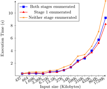
The first series of Figure 8 (square points) shows the execution time of the taxi app as a function of its input size. Larger file sizes were obtained by replicating the input file from DIBS multiple times. Mindful of the relationship between abstraction penalty and region size, we then investigated how the input data in the taxi app determined SIMD occupancy. Input lines have an average length of 1397 characters, so regions corresponding to each line in the stage 1 are large, and the penalty to occupancy is expected to be low. In contrast, lines contain on average only 45 coordinate pairs, less than the SIMD width, and so would be expected to incur a large penalty to occupancy in stage 2, whose region size is determined by the number of pairs per line. Indeed, we found that stage 1 was fired with full SIMD ensembles 91% of the time, while stage 2 had full ensembles only 9% of the time.
When regional context changes frequently relative to the SIMD width, the occupancy cost to performance of our implementation may exceed the cost (mainly extra memory accesses) of replicating this context along with every data item. We therefore developed a second version of the taxi app that used enumeration to provide context in stage 1 but explicitly marked each open-brace with its line's tag before sending it to stage 2. The latter stage does not utilize the enumeration abstraction and so can process items from multiple lines in one ensemble, achieving essentially full SIMD occupancy. The second series in Figure 8 (triangular points) shows that improved occupancy results in lower total execution time. However, using the same strategy to tag each character of each line in stage 1, while it slightly improves occupancy by avoiding enumeration entirely, incurs substantially more overhead due to the much greater number of elements to be tagged per region. The third series (x points) shows that, at the largest input size tested, a pure tagging implementation is roughly 30% slower than one that judiciously uses either tagging or our design as appropriate for each stage.
We conclude that the best way to provide regional context to streaming applications on a SIMD architecture depends strongly on the performance tradeoff between reduced SIMD occupancy and reduced representation overhead. Each stage of a pipeline may represent a different point in this tradeoff, and the highest-performing implementation (dense or sparse) for regional context may
Fig. 8. Execution time vs input size for three versions of the taxi app.
<details>
<summary>Image 6 Details</summary>
### Visual Description
\n
## Line Chart: Execution Time vs. Input Size
### Overview
This line chart depicts the relationship between execution time (in seconds) and input size (in kilobytes) for three different enumeration strategies. The chart shows how the execution time increases with increasing input size for each strategy.
### Components/Axes
* **X-axis:** Input size (Kilobytes). Marked with values: 437, 864, 1.69K, 3.38K, 6.75K, 13.5K, 27K, 5.4K, 108K, 216K, 432K, 864K, 1728K.
* **Y-axis:** Execution Time (s). Scale ranges from approximately 0 to 10 seconds.
* **Legend:** Located in the top-left corner. Contains three lines with corresponding labels:
* "Both stages enumerated" (Blue squares)
* "Stage 1 enumerated" (Red triangles)
* "Neither stage enumerated" (Orange diamonds)
### Detailed Analysis
* **Both stages enumerated (Blue):** The line starts at approximately 0.8s at 437KB, increases slowly until around 216KB, then rises sharply to approximately 9.2s at 1728KB. The trend is generally upward, with a steeper slope at larger input sizes.
* 437KB: ~0.8s
* 864KB: ~1.1s
* 1.69K: ~1.2s
* 3.38K: ~1.4s
* 6.75K: ~1.6s
* 13.5K: ~1.8s
* 27K: ~2.1s
* 5.4K: ~2.2s
* 108K: ~2.8s
* 216K: ~3.3s
* 432K: ~4.6s
* 864K: ~6.3s
* 1728K: ~9.2s
* **Stage 1 enumerated (Red):** The line starts at approximately 0.7s at 437KB, increases steadily to approximately 4.4s at 432KB, and then increases rapidly to approximately 8.3s at 1728KB. The trend is also upward, but generally slower than the "Both stages enumerated" line until around 432KB.
* 437KB: ~0.7s
* 864KB: ~0.9s
* 1.69K: ~1.1s
* 3.38K: ~1.3s
* 6.75K: ~1.6s
* 13.5K: ~1.9s
* 27K: ~2.3s
* 5.4K: ~2.4s
* 108K: ~3.1s
* 216K: ~3.8s
* 432K: ~4.4s
* 864K: ~6.7s
* 1728K: ~8.3s
* **Neither stage enumerated (Orange):** The line starts at approximately 0.6s at 437KB, increases gradually to approximately 3.8s at 432KB, and then increases very rapidly to approximately 11.3s at 1728KB. This line consistently shows the highest execution times, especially at larger input sizes.
* 437KB: ~0.6s
* 864KB: ~0.8s
* 1.69K: ~0.9s
* 3.38K: ~1.1s
* 6.75K: ~1.3s
* 13.5K: ~1.6s
* 27K: ~1.9s
* 5.4K: ~2.1s
* 108K: ~2.8s
* 216K: ~3.4s
* 432K: ~3.8s
* 864K: ~5.8s
* 1728K: ~11.3s
### Key Observations
* The execution time increases with input size for all three enumeration strategies.
* "Neither stage enumerated" consistently exhibits the longest execution times, particularly as the input size grows.
* "Both stages enumerated" and "Stage 1 enumerated" have similar performance for smaller input sizes, but "Both stages enumerated" becomes more efficient at larger input sizes.
* The increase in execution time appears to be exponential for all strategies as input size increases beyond 432KB.
### Interpretation
The data suggests that enumerating stages in the process significantly impacts execution time, especially for larger input sizes. The strategy of enumerating neither stage is the least efficient, indicating that enumeration provides a performance benefit. The fact that "Both stages enumerated" outperforms "Stage 1 enumerated" at larger input sizes suggests that enumerating both stages provides a more scalable solution. The exponential increase in execution time with input size indicates a potential bottleneck or algorithmic complexity that becomes more pronounced as the input grows. This could be due to the overhead of enumeration becoming more significant with larger datasets, or due to the underlying algorithm's time complexity. The chart highlights the importance of choosing an appropriate enumeration strategy to optimize performance, particularly when dealing with large input sizes. The data points suggest that the performance difference between the strategies is negligible for very small inputs, but becomes substantial as the input size increases.
</details>
therefore vary between stages. Ultimately, this choice should be made transparently to the application developer based on profile-guided feedback.
## 6 Conclusion and Future Work
We have described an abstraction, enumeration and aggregation, to support stateful streaming computation based on regional contexts. We presented an implementation of this abstraction for irregular streaming computations on SIMDparallel architectures such as GPUs. Our abstraction relies on a sparse implementation of precise signal delivery between computational stages.
We characterized the cost of the abstraction on benchmark computations and demonstrated that the best strategy for realizing it may depend on the relationship between region size and the architecture's SIMD width. Future work will include more careful modeling and/or empirical measurement of the costs of alternative implementations, with an eye toward allowing the MERCATOR runtime to transparently choose between strategies based on the typical number of elements per region.
Another direction for future work will investigate how to lower the abstraction penalty of precise signaling for SIMD occupancy. When the effects of a signal on a node's state are limited and well-defined (e.g. changing the parent object pointer), the node may be able to compute the correct state (pre- or post-signal) to expose to the item in each SIMD lane separately. Computing the correct state per item in each node, rather than storing it with items in the queues between nodes, would offer the same efficient representation of state as in our design while eliminating signals' cost to SIMD occupancy.
## Acknowledgments
This work was supported by NSF CISE awards CNS-1763503 and CNS-1500173.
## References
1. Altschul, S., Gish, W., Miller, W., Myers, E., Lipman, D.: Basic local alignment search tool. J. Molecular Biology 215 (3), 403-10 (1990)
2. Barnes, J., Hut, P.: A hierarchical o(n log n) force-calculation algorithm. Nature 324 (6096), 446 (1986)
3. Cabrera, A.M., Faber, C.J., Cepeda, K., Derber, R., Epstein, C., Zheng, J., Cytron, R.K., Chamberlain, R.D.: DIBS: A data integration benchmark suite. In: 2018 ACM/SPEC Int'l Conf. Performance Engineering. pp. 25-28 (2018)
4. Chamberlain, R., Franklin, M., Tyson, E., Buckley, J., et al.: Auto-Pipe: streaming applications on architecturally diverse systems. Computer 43 (3), 42-49 (2010)
5. Cole, S., Buhler, J.: MERCATOR: A GPGPU framework for irregular streaming applications. In: 2017 Int'l Conf. High Performance Computing and Simulation. pp. 727-36 (2017)
6. Eker, J., Janneck, J., Lee, E.A., Liu, J., Ludvig, J., Sachs, S., , Xiong, Y.: Taming heterogeneity - the Ptolemy approach. Proc. IEEE 91 (1), 127-44 (2003)
7. Grossman, M., Simion Sbˆ ırlea, A., Budimli´ c, Z., Sarkar, V.: CnC-CUDA: Declarative programming for GPUs. In: Cooper, K., Mellor-Crummey, J., Sarkar, V. (eds.) Languages and Compilers for Parallel Computing. pp. 230-245. Springer Berlin (2011)
8. Lee, E., Messerschmitt, D.: Synchronous data flow. Proc. IEEE 75 (9), 1235-245 (1987)
9. Li, P., Agrawal, K., Buhler, J., Chamberlain, R.: Orchestrating safe streaming computations with precise control. In: 4th Int'l Workshop on Extreme Scale Computing Application Enablement - Modeling and Tools. pp. 1017-22 (2014)
10. Roesch, M., et al.: Snort: Lightweight intrusion detection for networks. In: Proc. 13th Systems Administration Conf. (LISA). pp. 229-238 (1999)
11. Thies, W., Karczmarek, M., Amaransinghe, S.: StreamIt: A language for streaming applications. In: 11th Int'l Conf. Compiler Construction. pp. 179-96 (2002)
12. Thies, W., Karczmarek, M., Sermulins, J., Rabbah, R., Amaransinghe, S.: Teleport messaging for distributed stream programs. In: 10th ACM SIGPLAN Symp. Principles and Practice of Parallel Programming. pp. 224-35 (2005)
13. Tyson, E., Buckley, J., Franklin, M., Chamberlain, R.D.: Acceleration of atmospheric Cherenkov telescope signal processing to real-time speed with the AutoPipe design system. Nuclear Instruments and Methods in Physics Research Sec. A: Accelerators, Spectrometers, Detectors and Associated Equipment 595 (2), 474-9 (2008)
14. Viola, P., Jones, M.: Rapid object detection using a boosted cascade of simple features. In: Proc. IEEE Comp. Soc. Conf. Computer Vision and Pattern Recognition (2001)
15. Zaharia, M., Chowdhury, M., Das, T., Dave, A., et al.: Resilient distributed datasets: A fault-tolerant abstraction for in-memory cluster computing. In: 9th USENIX Conf. Networked Systems Design and Implementation. p. 2 (2012)
16. Zaharia, M., Xin, R., Wendell, P., Das, T., Armbrust, M., Dave, A., Meng, X., Rosen, J., Venkataraman, S., Franklin, M., Ghodsi, A., Gonzalez, J., Shenker, S., Stoica, I.: Apache Spark: a unified engine for big data processing. Communications of the ACM 59 (11), 56-65 (2016)
## 7 Appendix: Proofs Omitted in Text
## 7.1 Proof of Lemma 1
Proof. We proceed by induction on the number of signals already on the signal queue S when s is emitted.
Suppose S is empty when n 1 emits s . All items emitted by n 1 prior to s either have been consumed by n 2 or are present on Q . The protocol assigns s an amount of credit equal to the size of Q . This amount is then added to n 2 's current credit counter, which was previously 0. Finally, n 2 consumes s precisely when its current credit counter returns to 0, which happens once n 2 consumes the items that were present on Q when s was emitted.
Now suppose s is emitted when S is not empty. s receives a number of credits equal to the number of items added to Q since the prior signal s ′ . We know inductively that n 2 consumes s ′ precisely when all data items emitted prior to s ′ have been consumed. At this point, the only items on Q must be those emitted after s ′ but before s , and n 2 's current credit counter is 0 since it just consumed a signal. Conclude that n 2 will transfer the credit in s to its current credit counter and will then consume exactly those data items emitted after s ′ but before s before it consumes s itself.
## 7.2 Proof of Lemma 2
Proof. Our proof of deadlock-freedom relies on the following two claims.
Claim. A node cannot have a current credit counter > 0 without a pending data item.
Proof of claim : Suppose that a node's current credit counter is > 0. The credit in the current counter was transferred from the signal s currently at the head of the signal queue; it cannot remain from prior signals because the node did not even check for s until its current credit counter last became 0. Hence, this credit was assigned to s to cover data items that were enqueued at the time that s was issued. Since not all credit has yet been consumed, at least one of these items is still enqueued.
Claim. If a node n has either pending data or a pending signal, one of the following holds: (1) n can consume a data item; (2) n can consume a signal; (3) n is blocked due to insufficient space in its downstream queues.
Proof of claim : The node either has credit or not. If it has credit, then by the previous claim it has pending data that can be consumed. If it has no credit but has a pending signal, then either the signal can be consumed, or credit can be transferred from the signal; in the latter case, there must again be data corresponding to this credit. If there is no credit and no pending signal, then there must be pending data, which can be consumed without credit in the absence of pending signals. In all cases, the node can consume some input unless its downstream queues lack sufficient space.
We now proceed to prove the original lemma. If any node in the pipeline has pending data or a signal, then let n be the last such node. Either n 's downstream queues are empty (else its successor would have pending data or signals), or n has no successor, i.e., it is the last node in the pipeline, which has unbounded output space and cannot block. Hence, node n is not blocked on its downstream queues and so, by the second claim, can be fired to consume input.
We conclude that the application terminates only when all nodes have exhausted their inputs.