## Explainable Automated Reasoning in Law using Probabilistic Epistemic Argumentation
Inga Ibs 1 , Nico Potyka 2
1 Technical University of Darmstadt 2 University of Stuttgart inga.ibs@tu-darmstadt.de, nico.potyka@ipvs.uni-stuttgart.de
## Abstract
Applying automated reasoning tools for decision support and analysis in law has the potential to make court decisions more transparent and objective. Since there is often uncertainty about the accuracy and relevance of evidence, non-classical reasoning approaches are required. Here, we investigate probabilistic epistemic argumentation as a tool for automated reasoning about legal cases. We introduce a general scheme to model legal cases as probabilistic epistemic argumentation problems, explain how evidence can be modeled and sketch how explanations for legal decisions can be generated automatically. Our framework is easily interpretable, can deal with cyclic structures and imprecise probabilities and guarantees polynomial-time probabilistic reasoning in the worstcase.
## 1 Introduction
Legal reasoning problems can be addressed from different perspectives. From a lawyer's perspective, a trial may be best modeled as a strategic game. In a criminal trial, for example, the prosecutor may try to convince the judge or jury of the defendant's guilt while the defense attorney tries the opposite. The problem is then to interpret the law and the evidence in a way that maximizes the agent's utility. From this perspective, a legal reasoning problem is best modeled using tools from decision and game theory (Hanson, Hanson, and Hart 2014; Prakken and Sartor 1996; Riveret et al. 2007).
Our focus here is not on strategic considerations, but on the decision process that leads to the final verdict in a legal process like a trial. Given different pieces of evidence and beliefs about their authenticity and relevance, how can we merge them to make a plausible and transparent decision? Different automated reasoning tools have been applied in order to answer similar questions, for example, casebased reasoning (Bench-Capon and Sartor 2003; McCarty 1995), argumentation frameworks (Dung and Thang 2010; Prakken et al. 2013) or Bayesian networks (Fenton, Neil, and Lagnado 2013). Since lawyers and judges often struggle with the interpretation of Bayesian networks, recent work also tries to explain Bayesian networks by argumentation tools (Vlek et al. 2016).
Here, we investigate the applicability of the probabilistic epistemic argumentation framework developed in (Hunter
2013; Hunter, Polberg, and Thimm 2018; Hunter and Thimm 2016; Thimm 2012). As opposed to classical argumentation approaches, this framework allows expressing uncertainty by means of probability theory. In particular, we can compute reasoning results in polynomial time when we restrict the language (Potyka 2019). As it turns out, the resulting fragment is sufficiently expressive for our purpose, so that our framework is computationally more efficient than many other probabilistic reasoning approaches that suffer from exponential runtime in the worst-case. At the same time, the graphical structure is easily interpretable and allows to automatically generate explanations for the final degrees of belief (probabilities) as we will explain later.
While we can incorporate objective probabilities in our framework, our probabilistic reasoning is best described as subjective in the sense that we basically merge beliefs about pieces of evidence and hypotheses (probabilities that can be either objective or subjective). In order to define the beliefs about pieces of evidence from objective evidence and statistical information, another approach like Bayesian networks or more general tools from probability theory may be better suited. Our framework can then be applied on top of these tools. In this sense, our framework can be seen as a complement rather than a replacement of alternative approaches.
The remainder of this paper is structured as follows: Section 2 explains the necessary basics. We will introduce a basic legal argumentation framework in Section 3 and discuss more sophisticated building blocks in Section 4. We will discuss and illustrate the explainability capabilities of our approach as we proceed, but explain some more general ideas in Section 5. Finally, we add some discussion about related work, the pros and cons of our framework and future work in Sections 6 and 7.
## 2 Probabilistic Epistemic Argumentation Basics
Our legal reasoning approach builds up on the probabilistic epistemic argumentation approach developed in (Thimm 2012; Hunter 2013; Hunter and Thimm 2016; Hunter, Polberg, and Thimm 2018). In this approach, we assign degrees of belief in the form of probabilities to arguments using probability functions over possible worlds. A possible world basically interprets every argument as either accepted or rejected. In order to restrict to probability functions that respect prior beliefs and the structure of the argumentation graph, different constraints can be defined. Afterwards, we can assign a probability interval to every argument based on these constraints. We will restrict to a fragment of the constraint language here that allows polynomial-time computations (Potyka 2019).
Formally, we represent arguments and their relationships in a directed edge-weighted graph ( A , E , w) . A is a finite set of arguments, E ⊆ A×A is a finite set of directed edges between the arguments and w : E → Q assigns a rational number to every edge. If there is an edge ( A,B ) ∈ E , we say that A attacks B if w (( A,B )) < 0 and A supports B if w (( A,B )) > 0 . We let Att( A ) = { B ∈ A | ( B,A ) ∈ E , w (( A,B )) < 0 } be the set of attackers of an argument A and Sup( A ) = { B ∈ A | ( B,A ) ∈ E , w (( A,B )) > 0 } be the set of supporters.
A possible world is a subset of arguments ω ⊆ A . Intuitively, ω contains the arguments that are accepted in a particular state of the world. Beliefs about the true state of the world are modeled by rational-valued probability functions P : 2 A → [0 , 1] ∩ Q such that ∑ ω ∈ 2 A P ( ω ) = 1 . The restriction to probabilities from the rational numbers is for computational reasons only. In practice, it does not really mean any loss of generality because implementations usually use finite precision arithmetic. We denote the set of all probability functions over A by P A . The probability of an argument A ∈ A under P is defined by adding the probabilities of all worlds in which A is accepted, that is, P ( A ) = ∑ ω ∈ 2 A ,A ∈ ω P ( ω ) . P ( A ) can be understood as a degree of belief, where P ( A ) = 1 means complete acceptance and P ( A ) = 0 means complete rejection.
The meaning of attack and support relationships can be defined by means of constraints in probabilistic epistemic argumentation. For example, the Coherence postulate in (Hunter and Thimm 2016) intuitively demands that the belief in an argument is bounded from above by the belief of its attackers. Formally, a probability function P respects Coherence iff P ( A ) ≤ 1 -P ( B ) for all B ∈ Att( A ) . A more general constraint language has recently been introduced in (Hunter, Polberg, and Thimm 2018). Here, we will restrict to a fragment of this language that allows solving our reasoning problems in polynomial time (Potyka 2019). A linear atomic constraint is an expression of the form
$$c _ { 0 } + \sum _ { i = 1 } ^ { n } c _ { i } \cdot \pi ( A _ { i } ) \leq d _ { 0 } + \sum _ { i = 1 } ^ { m } d _ { i } \cdot \pi ( B _ { i } ) ,$$
where A i , B i ∈ A , c i , d i ∈ Q , n, m ≥ 0 (the sums can be empty) and π is a syntactic symbol that can be read as 'the probability of'. For example, the Coherence condition above can be expressed by a linear atomic constraint with m = n = 1 , c 0 = 0 , c 1 = 1 , A 1 = A , d 0 = 1 , d 1 = -1 and B 1 = B . However, we can also define more complex constraints that take the beliefs of more than just two arguments into account. Usually, the arguments that occur in a constraint are neighbors in the graph and the coefficients c i , d i will often be based on the weight of the edges between the arguments. We will see many examples later.
A probability function P satisfies a linear atomic constraint iff c 0 + ∑ n i =1 c i · P ( A i ) ≤ d 0 + ∑ m i =1 d i · P ( B i ) . P satisfies a set of linear atomic constraints C , denoted as P | = C , iff it satisfies all constraints c ∈ C . If this is the case, we call C satisfiable .
We are interested in two reasoning problems here that have been introduced in (Hunter and Thimm 2016). First, the satisfiability problem is, given a graph ( A , E , w) and a set of constraints C over this graph, to decide if the constraints are satisfiable. This basically allows us to check that our modelling assumptions are consistent. Second, the entailment problem is, given a graph ( A , E , w) , a set of satisfiable constraints C and an argument A , to compute lower and upper bounds on the probability of A based on the probability functions that satisfy the constraints. For example, suppose we have A = { A,B,C } , E = { ( A,B ) , ( B,C ) } , w(( A,B )) = 1 , w(( B,C )) = -1 . We encode the meaning of the support relationship ( A,B ) by w (( A,B )) · π ( A ) ≤ π ( B ) (a supporter bounds the belief in the argument from below) and the meaning of the attack relationship ( B,C ) by π ( C ) ≤ 1 + w (( B,C )) · P ( B ) (an attacker bounds the belief in the argument from above). Say, we also tend to accept C and model this by the constraint 0 . 5 ≤ π ( C ) . Then our constraints are satisfiable and the entailment results are P ( A ) ∈ [0 , 0 . 5] , P ( B ) ∈ [0 , 0 . 5] , P ( C ) ∈ [0 . 5 , 1] . To understand the reasoning, let us consider the upper bound for A . If we had P ( A ) > 0 . 5 , we would also have P ( B ) > 0 . 5 because of the support constraint. But then, we would have P ( C ) < 0 . 5 because of the attack constraint. However, this would violate our constraint for C . Hence, we must have P ( A ) ≤ 0 . 5 . In particular, if we would add the constraint 1 ≤ π ( A ) (accept A ), our constraints would become unsatisfiable. Both the satisfiability and the entailment problem can be automatically solved by linear programming techniques. In general, the linear programs can become exponentially large. However, both problems can be solved in polynomial time when we restrict to linear atomic constraints (Potyka 2019).
## 3 Basic Legal Argumentation Framework
Legal reasoning problems can occur in many forms and an attempt to capture all of them at once would most probably result in a framework that is hardly more concrete than a general abstract argumentation framework. We will therefore focus on a particular scenario, where the innocence of a defendant has to be decided. Modeling a single case may not be sufficient to illustrate the general applicability of probabilistic epistemic argumentation. We will therefore try to define a reasoning framework that can be instantiated for different cases, while still being easily comprehensible. As with every formal model, there are some simplifying assumptions about the nature of a trial. However, we think that our framework is sufficient to illustrate how real cases can be modeled and structured by means of probabilistic epistemic argumentation. We will make some additional comments about this as we proceed.
Following (Fenton, Neil, and Lagnado 2013), we regard a legal case roughly as a collection of hypotheses and pieces of evidence that support the hypotheses. We model both as
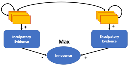
Figure 1: Meta-Graph for our Legal Reasoning Framework.
<details>
<summary>Image 1 Details</summary>
### Visual Description
\n
## Diagram: Causal Loop Diagram - Evidence and Innocence
### Overview
The image presents a causal loop diagram illustrating the relationship between inculpatory evidence, exculpatory evidence, and a belief in innocence. The diagram uses rounded rectangles to represent variables and arrows to indicate causal relationships, with "+" and "-" signs denoting positive and negative influences, respectively. The central variable is "Innocence," with "Max" written above it.
### Components/Axes
The diagram consists of the following components:
* **Innocence:** A large, oval-shaped node in the center, colored blue.
* **Inculpatory Evidence:** A rectangular node on the left, colored blue.
* **Exculpatory Evidence:** A rectangular node on the right, colored blue.
* **Evidence Stacks:** Two stacks of smaller, rectangular nodes colored yellow, positioned above "Inculpatory Evidence" and "Exculpatory Evidence" respectively. These represent the accumulation of evidence.
* **Arrows:** Black arrows indicating causal relationships.
* **Signs:** "+" and "-" signs along the arrows, indicating positive and negative influences.
* **Text:** "Max" positioned above the "Innocence" node.
### Detailed Analysis / Content Details
The diagram shows the following causal relationships:
1. **Inculpatory Evidence -> Innocence:** A negative influence ("-") indicates that an increase in inculpatory evidence *decreases* belief in innocence.
2. **Exculpatory Evidence -> Innocence:** A positive influence ("+") indicates that an increase in exculpatory evidence *increases* belief in innocence.
3. **Innocence -> Inculpatory Evidence:** A positive influence ("+") indicates that a stronger belief in innocence *increases* the search for or interpretation of inculpatory evidence.
4. **Innocence -> Exculpatory Evidence:** A negative influence ("-") indicates that a stronger belief in innocence *decreases* the search for or interpretation of exculpatory evidence.
5. **Evidence Stacks -> Inculpatory/Exculpatory Evidence:** Arrows from the yellow evidence stacks to the respective evidence nodes indicate that the accumulation of evidence influences the amount of that type of evidence.
6. **Loops:** There are two feedback loops:
* A reinforcing loop between Innocence, Inculpatory Evidence, and back to Innocence.
* A balancing loop between Innocence, Exculpatory Evidence, and back to Innocence.
### Key Observations
The diagram illustrates a system where belief in innocence can be self-reinforcing (through seeking out inculpatory evidence) or self-correcting (through seeking out exculpatory evidence). The presence of "Max" above "Innocence" suggests a potential upper limit or threshold for the belief in innocence. The diagram highlights the potential for confirmation bias, where existing beliefs influence the interpretation of evidence.
### Interpretation
This diagram represents a simplified model of how evidence influences perceptions of guilt or innocence. The positive feedback loop involving inculpatory evidence suggests that once a belief in guilt begins to form, it can be reinforced by selectively attending to evidence that supports that belief. Conversely, the balancing loop involving exculpatory evidence suggests that a strong belief in innocence can lead to a search for evidence that confirms that belief, potentially mitigating the impact of incriminating evidence. The "Max" label implies that there is a limit to how strongly someone can believe in innocence, even in the face of overwhelming evidence. This model is relevant to understanding biases in legal proceedings, investigations, and everyday decision-making. The diagram is a conceptual model and does not provide quantitative data. It is a qualitative representation of causal relationships.
</details>
abstract arguments, that is, as something that can be accepted or rejected to a certain degree by a legal decision maker like a judge, the jury or a lawyer. To begin with, we introduce three meta hypotheses that we model by three arguments E inc (the defendant should be declared guilty because of the inculpatory evidence), E ex (the defendant should be declared innocent because of the exculpatory evidence) and Innocence (the defendant is innocent). We regard Innocence as the ultimate hypothesis that is to be decided within the trial. In general, it may be necessary to consider several ultimate hypotheses that may correspond to different qualitative degrees of legal liability (e.g. intent vs. accident vs. innocent). If necessary, these can be incorporated by adding additional ultimate hypotheses in an analogous way. E inc and E ex are supposed to merge hypotheses and pieces of evidence that speak against ( E inc ) or for ( E ex ) the defendant's innocence as illustrated in Figure 1. Support relationships are indicated by a plus and attack relationships by a minus sign. There can also be attack and support relationships between pieces of evidence and additional hypotheses.
Intuitively, as our belief in E inc increases, our belief in Innocence should decrease. As our belief in E ex increases, our belief in Innocence should increase. From a classical perspective, accepting E inc , should result in rejecting Innocence and accepting E ex , should result in accepting Innocence . In particular, we should not accept E ex and E inc at the same time. Of course, in general, both the inculpatory evidence and the exculpatory evidence can be convincing to a certain degree. Probabilities are one natural way to capture this uncertainty. Intuitively, our basic framework is based on the following assumptions that we will make precise in the subsequent definition.
Inculpatory Evidence (IE): The belief in Innocence is bounded from above by the belief in E inc .
Exculpatory Evidence (EE): The belief in Innocence is bounded from below by the belief in E ex .
Supporting Evidence (SE): The belief in E inc and E ex is bounded from below by the belief in their supporting pieces of evidence.
Presumption of Innocence (PI): The belief in Innocence is the maximum belief that is consistent with all assumptions.
The following definition gives a more formal description of our framework. Our four main assumptions are formalized in items 4 and 5.
Definition 1 (Basic Legal Argumentation Framework (BLAF)) . A BLAF is a quadruple ( A , E , w , C ) , where A is a finite set of arguments, E is a finite set of directed edges between the arguments, w : E → Q is a weighting function and C is a set of linear atomic constraints over A such that:
1. A = A M A S A E is partitioned into a set of metahypotheses A M = { Innocence , E inc , E ex } , a set of subhypotheses A S and a set of pieces of evidence A E .
2. E = E M E S E E is partitioned into a set of meta edges E M = { (E inc , Innocence) , (E ex , Innocence) } , a set of support edges E S ⊆ ( A S ∪ A E ) ×{ E inc , E ex } and a set of evidential edges E E ⊆ ( A S ∪ A E ) × ( A S ∪ A E ) .
3. w((E inc , Innocence)) = -1 and w((E ex , Innocence)) = 1 . Furthermore, 0 ≤ w( e ) ≤ 1 for all e ∈ E S
4. C contains at least the following constraints:
5. IE: π (Innocence) ≤ 1+w((E inc , Innocence)) · π (E inc ) ,
6. EE: w((E ex , Innocence)) · π (E ex ) ≤ π (Innocence) ,
7. SE: w(( E,H )) · π ( E ) ≤ π ( H ) for all ( E,H ) ∈ E S .
5. For all A ∈ A , we call B ( A ) = min P | = C P ( A ) the lower belief in A and B ( A ) = max P | = C P ( A ) the upper belief in A . The belief in Innocence in is defined as
$$P I \colon \mathcal { B } ( I n n o c e n c e ) = \mathcal { B } ( A ) .$$
and the belief in the remaining A ∈ A \ { Innocence } is the interval B ( A ) = [ B ( A ) , B ( A )] .
Items 1-3 basically give a more precise description of the graph illustrated in Figure 1. Item 4 encodes our first three main assumptions as linear atomic constraints. The general form of our basic constraints is π ( B ) ≤ 1 + w (( A,B )) · P ( A ) for attack relations ( A,B ) (note that for w (( A,B )) = -1 , this is just the coherence constraint from (Hunter and Thimm 2016)) and w (( A,B )) · π ( A ) ≤ π ( B ) for support relations. Intuitively, attacker bound beliefs from above and supporter bound beliefs from below. Item 5 defines lower and upper beliefs in arguments as the minimal and maximal probabilities that are consistent with our constraints. Following our fourth assumption (presumption of innocence), the belief in Innocence is defined by the upper bound. The beliefs in the remaining arguments is the interval defined by the lower and upper bound. The following proposition summarizes some consequences of our basic assumptions.
Proposition 1. For every BLAF ( A , E , w , C ) , we have
1. B (E inc ) ≤ 1 -B (E ex ) and B (E ex ) ≤ 1 -B (E inc ) .
2. For all support edges ( a, E ) ∈ E S , we have
- B (E ex ) ≤ 1 -w(( a, E inc )) · B ( a ) if E = E inc ,
- B (E inc ) ≤ 1 -w(( a, E ex )) · B ( a ) if E = E ex .
Proof. 1. We prove only the first statement, the second one follows analogously. Consider an arbitrary P ∈ P A that satisfies C . Then P (E inc ) ≤ P (Innocence) ≤ 1 -P (E ex ) ≤ 1 - B (E ex ) . The first inequality follows from EE and the second from IE (Def. 1, item 4) along with the conditions
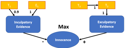
Figure 2: BLAF for Example 1.
<details>
<summary>Image 2 Details</summary>
### Visual Description
\n
## Diagram: Evidence and Innocence Model
### Overview
This diagram illustrates a model relating different types of evidence (incriminating and exculpatory) to a conclusion of innocence. It uses boxes to represent evidence categories and an oval to represent the outcome (innocence). Arrows indicate relationships and are labeled with numerical values representing the strength of the connection. The diagram appears to be a simplified representation of a Bayesian network or similar probabilistic reasoning model.
### Components/Axes
The diagram consists of the following components:
* **T1:** A yellow box labeled "T1".
* **E1:** A yellow box labeled "E1".
* **T2:** A yellow box labeled "T2".
* **T3:** A yellow box labeled "T3".
* **Incriminating Evidence:** A blue rectangle labeled "Incriminating Evidence".
* **Exculpatory Evidence:** A blue rectangle labeled "Exculpatory Evidence".
* **Innocence:** A blue oval labeled "Innocence".
* **Max:** Text label "Max" positioned centrally between the "Incriminating Evidence" and "Exculpatory Evidence" boxes.
* **Arrows:** Arrows connecting the boxes and oval, with numerical labels indicating the strength of the relationship.
* **"+" and "-":** Symbols indicating positive and negative influence on "Innocence".
### Detailed Analysis or Content Details
The diagram shows the following relationships:
* An arrow connects "T1" to "Incriminating Evidence" with a label of "0.9".
* An arrow connects "E1" to "Incriminating Evidence" with a label of "1".
* An arrow connects "T2" to "T3" with a label of "1".
* An arrow connects "T3" to "Exculpatory Evidence" with a label of "1".
* An arrow connects "Incriminating Evidence" to "Innocence" with a "-" symbol, indicating a negative influence.
* An arrow connects "Exculpatory Evidence" to "Innocence" with a "+" symbol, indicating a positive influence.
### Key Observations
The diagram suggests that incriminating evidence (formed from T1 and E1) decreases the likelihood of innocence, while exculpatory evidence (formed from T2 and T3) increases it. The numerical labels suggest that E1 has a stronger influence on incriminating evidence than T1 (1 vs 0.9). The connections between T2, T3, and Exculpatory Evidence are all at maximum strength (1).
### Interpretation
This diagram represents a simplified model of how evidence contributes to a determination of innocence. The "Max" label suggests a maximization process, potentially indicating that the model aims to maximize the probability of innocence given the available evidence. The diagram implies that the strength of the evidence (represented by the numerical labels) directly impacts the conclusion of innocence. The model is a conceptual illustration and does not provide specific quantitative details about how the evidence is combined or how the final determination of innocence is made. The diagram is a visual representation of a logical argument, where the presence of incriminating evidence weakens the case for innocence, and the presence of exculpatory evidence strengthens it. The values assigned to the connections suggest a degree of confidence or weight given to each piece of evidence.
</details>
on w (Def. 1, item 3). The third inequality follows because B (E ex ) ≤ P (E ex ) by definition of B .
2. Again, we prove only the first statement. Note that SE (Def. 1, item 4) implies P (E inc ) ≥ w(( a, E inc )) · P ( a ) for all P ∈ P A that satisfy C . Therefore, P (E ex ) ≤ 1 -P (E inc ) ≤ 1 -w(( a, E inc )) · P ( a ) ≤ 1 -w(( a, E inc )) ·B ( a ) , where the first and third inequalities can be derived like in 1.
Intuitively, item 1 says that our upper belief that the defendant should be declared guilty because of the inculpatory evidence is bounded from above by our lower belief that the defendant should be declared innocent because of the exculpatory evidence and vice versa. By rearranging the equations, we can see that the lower belief in E inc is also bounded from above by the upper belief in E ex and vice versa. Item 2 explains that every argument a that directly contributes to inculpatory (exculpatory) evidence E gives an upper bound for the belief in E ex ( E inc ) that is based on our lower belief B ( a ) and the relevance w(( a, E )) of this argument. In a similar way, we could bound the beliefs in contributors to E inc by the belief in contributors to E ex by taking their respective weights into account. However, the general description becomes more and more difficult to comprehend. Therefore, we just illustrate the interactions by means of a simple example.
Example 1. Let us consider a simple case of hit-and-run driving. The defendant is accused of having struck a car while parking at a shopping center. The plaintiff witnessed the accident from afar and denoted the registration number from the licence plate when the car left ( T 1 ). The defendant denies the crime and testified that he was at home with his girlfriend at the time of the offence ( T 2 ). His girlfriend confirmed his alibi ( T 3 ). However, a security camera at the parking space recorded a person that bears strong resemblance to the defendant at the time of the crime ( E 1 ). We consider a simple formalization shown in Figure 2. We designed the graph in a way that allows illustrating the interactions in our framework. One may also want to regard T 3 as a supporter of exculpatory evidence and consider attack relationships between E 1 and T 1 and T 3 . We do not introduce such edges because we want to illustrate the indirect interactions between arguments. In this example, we may weigh all edges with 1 and control the uncertainty only about the degrees of belief. However, we assign a weight of 0 . 9 to the edge from T 1 in order to illustrate the effect of the weight. This may capture the uncertainty that the plaintiff may have written down the wrong registration number, for example. The
Table 1: Beliefs under additional assumptions for Example 1 (rounded to two digits). Directly constrained beliefs are highlighted in bold.
| A | B 1 | B 2 | B 3 |
|-----------|--------|------------|------------|
| Innocence | 1 | 1 | 0.1 |
| E inc | [0, 1] | [0, 0.3] | [0.9, 1] |
| E ex | [0, 1] | [0.7, 1] | [0, 0.1] |
| T 1 | [0, 1] | [0, 0.33] | [0, 1] |
| T 2 | [0, 1] | [0.7, 1] | [0, 0.1] |
| T 3 | [0, 1] | [ 0.7 , 1] | [0, 0.1] |
| E 1 | [0, 1] | [0, 0.3] | [ 0.9 , 1] |
probability for T 1 , T 2 and T 3 is our degree of belief that the corresponding testimonies are true. The probability of E 1 is our degree of belief that the camera does indeed show the defendant and not just another person. Without additional assumptions, we can only derive that our degree of belief in Innocence is 1 (presumption of innocence) as shown in the second column ( B 1 ) of Table 1. We could now start adding assumptions and looking at the consequences. For example, let us assume that the statement of the defendant's girlfriend was very convincing. We could incorporate this by adding the constraint π ( T 3 ) ≥ 0 . 7 . The consequences are shown in the third column ( B 2 ) of Table 1. However, if the person on the camera bears strong resemblance to the defendant, we may find that the upper belief in E 1 is too low. This means that our assumption is too strong and needs to be revised. Let us just delete the constraint π ( T 3 ) ≥ 0 . 7 and instead impose a constraint on E 1 . Let us assume that there is hardly any doubt that the camera shows the defendant. We could incorporate this by adding the constraint π ( E 1 ) ≥ 0 . 9 . The consequences are shown in the fourth column ( B 3 ) of Table 1.
The choice of probabilities (degrees of belief), weights (relevance) and additional attack or support relations is, of course, subjective. However, arguably, every court decision is subjective in that the decision maker(s) have to weigh the plausibility and the relevance of the evidence in one way or another. By making these assumptions explicit in a formal framework, the decision process can become more transparent. Furthermore, by computing probabilities while adding assumptions, possible inconsistencies can be detected and resolved early. Since we restrict to linear atomic constraints, computing probabilities can be done within a second even when there are thousands of arguments.
Let us note that our framework also allows defining some simple rules that allow deriving explanations for the verdict automatically. For example, the belief in Innocence can be explained directly from the beliefs in E inc and E ex . If both B (E inc ) ≤ 0 . 5 and B (E ex ) ≤ 0 . 5 . our system may report that the defendant is found innocent because of lack of evidence. If B (E ex ) > 0 . 5 , it could report that the defendant is found innocent because the exculpatory evidence is more plausible than the inculpatory evidence (recall from Proposition 1 that B (E inc ) ≤ 1 -B (E ex ) ). Finally, if B (E inc ) is sufficiently large, it could report that the defendant is found guilty because of the inculpatory evidence. The belief in E inc and E ex can then be further explained based on the belief in supporting hypotheses and pieces of evidence. The influence of supporting arguments can be measured by their lower belief bounds and their weight. To illustrate this, consider again Table 1. For B 1 , the system could report that the defendant is innocent because of lack of convincing evidence, while, for B 2 , it can explain that there is convincing exculpatory evidence. If desired, it can then further report T 2 as the direct explanation and, going backwards, T 3 as an additional explanation. Similarly, for B 3 , the system could report that the defendant is probably not innocent because of the inculpatory evidence. Again, the system could give further explanations by going backwards in the graph. We will discuss the idea in more general form in Section 5.
## 4 Adding Additional Structure to BLAFs
BLAFs can capture a wide variety of cases. However, it is often desirable to add additional structure that captures recurring patterns in legal reasoning. From a usability perspective, this makes the graph more easily comprehensible and allows modeling different cases in a consistent and standardized way. From an automated reasoning perspective, it allows adding additional general rules that can automatically derive explanations for decisions.
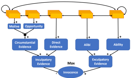
Two natural subsets of inculpatory evidence are direct ( E d ) and circumstantial ( E c ) inculpatory evidence. While direct evidence provides direct inculpatory evidence, circumstantial evidence involves indirect evidence that requires multiple inferential steps (Fenton, Neil, and Lagnado 2013). For example, a camera that recorded the defendant while committing the crime can be seen as direct evidence, while a camera that recorded the defendant close to the crime scene like in Example 1 can be seen as a piece of circumstantial evidence. Two prominent categories of circumstantial evidence are motive (the defendant had a reason to commit the crime) and opportunity (the defendant had the opportunity to commit the crime). Figure 3 shows a refined BLAF. As indicated by the join of their support edges, the beliefs in pieces of circumstantial evidence are merged and not considered independently. Only if both a motive and the opportunity (and perhaps some additional conditions) were present, the defendant should be found guilty. In contrast, pieces of direct evidence are standalone arguments for the defendant's guilt.
Two recurring patterns of exculpatory evidence are alibi and ability . While an alibi indicates that the defendant has not been at the crime scene at the time of the crime, ability can contain pieces of evidence that indicate that the defendant could not have committed the crime, for example, due to lack of physical strength. Figure 3 shows an extended BLAF with six additional meta-hypotheses. As before, we allow edges between all pieces of evidence and subhypotheses, but do not draw all possible direct connections in order to keep the graph comprehensible. The meaning of the support edges pointing to inculpatory and exculpatory evidence is already defined by SE in Definition 1, item 4. That is the corresponding support relations ( A,B ) are
Figure 3: Refined BLAF with additional meta-hypotheses.
<details>
<summary>Image 3 Details</summary>
### Visual Description
\n
## Diagram: Evidence and Innocence Model
### Overview
The image presents a diagram illustrating the relationship between various types of evidence (Motive, Opportunity, Circumstantial Evidence, Direct Evidence, Alibi, Ability, Inculpatory Evidence, Exculpatory Evidence) and the concept of Innocence. The diagram uses a flow-based structure with positive (+) and negative (-) indicators to show how each element influences the others. It appears to be a causal loop diagram, representing a system of reinforcing and balancing feedback loops.
### Components/Axes
The diagram consists of the following components:
* **Top Row:** Five yellow rectangular boxes labeled: "Motive", "Opportunity", "Direct Evidence", "Alibi", "Ability".
* **Middle Row:** Two blue rectangular boxes labeled: "Circumstantial Evidence", "Direct Evidence".
* **Bottom Row:** Two blue rectangular boxes labeled: "Inculpatory Evidence", "Exculpatory Evidence".
* **Central Box:** A blue circular box labeled: "Innocence".
* **Label:** "Max" positioned above the "Innocence" box.
* **Arrows:** Arrows connecting the boxes, with "+" signs indicating a positive influence (increase) and no explicit negative signs, implying a negative influence (decrease).
* **Loops:** A curved arrow looping back from the last yellow box to the first, and another looping from "Innocence" to "Motive".
### Detailed Analysis / Content Details
The diagram shows the following relationships:
1. **Motive** positively influences **Circumstantial Evidence**.
2. **Opportunity** positively influences **Circumstantial Evidence** and **Direct Evidence**.
3. **Circumstantial Evidence** positively influences **Inculpatory Evidence**.
4. **Direct Evidence** positively influences **Inculpatory Evidence**.
5. **Alibi** positively influences **Exculpatory Evidence**.
6. **Ability** positively influences **Exculpatory Evidence**.
7. **Inculpatory Evidence** positively influences **Innocence** (but the diagram suggests this is a negative influence, as it reduces innocence).
8. **Exculpatory Evidence** positively influences **Innocence**.
9. A feedback loop exists from **Motive** to **Opportunity** to the other yellow boxes, and back to **Motive**.
10. A feedback loop exists from **Innocence** to **Motive**.
The "+" signs indicate that an increase in the preceding element leads to an increase in the following element. The absence of "-" signs suggests that an increase in the preceding element leads to a decrease in the following element.
### Key Observations
* The diagram highlights the interplay between different types of evidence in determining innocence.
* The feedback loops suggest that the system can be self-reinforcing (e.g., more motive leads to more circumstantial evidence, which further reinforces the motive) or self-correcting (e.g., exculpatory evidence increases innocence, potentially reducing the need for further investigation).
* The "Max" label above "Innocence" suggests a maximum level of innocence that can be established.
* The diagram does not provide quantitative data, but rather a qualitative representation of relationships.
### Interpretation
This diagram appears to be a conceptual model used in legal or investigative contexts. It illustrates how various pieces of evidence contribute to or detract from a person's presumed innocence. The positive and negative influences represent the strength and direction of the relationship between these elements.
The loops suggest that the system is dynamic and interconnected. For example, a strong motive can lead to the discovery of circumstantial evidence, which can further strengthen the motive. Conversely, strong exculpatory evidence can increase innocence, potentially leading to a re-evaluation of the initial motive.
The "Max" label suggests that there is a limit to how much innocence can be established, even with strong exculpatory evidence. This could be due to factors such as the burden of proof or the inherent uncertainty in legal proceedings.
The diagram is a simplified representation of a complex system, but it provides a useful framework for understanding the relationships between evidence and innocence. It could be used to guide investigations, evaluate evidence, or communicate the complexities of a case to others. The diagram is not providing facts or data, but a model of how these concepts relate.
</details>
associated with the constraint w (( A,B )) · π ( A ) ≤ π ( B ) . This constraint could also be naturally used for the evidential edges that point to direct evidence, alibi and ability. However, the circumstantial evidence patterns motive and opportunity should not act independently, but complement each other. Neither a motive, nor the opportunity alone, are a good reason to find the defendant guilty. However, if both a good motive and the opportunity are present, this may be a good reason. We say that both items together provide collective support for the guilt of the defendant. To formalize collective support , we can consider a constraint w((Motive , E c )) · π (Motive) + w((Opportunity , E c )) · π (Opportunity) ≤ π (E c ) such that w((Motive , E c )) + w((Opportunity , E c )) ≤ 1 . For example, we could set w((Motive , E c )) = w((Opportunity , E c )) = 0 . 4 . Then the presence of a strong motive or the opportunity alone cannot decrease the belief in the defendant's innocent by more than 0 . 4 and both together cannot decrease the belief by more than 0 . 8 . Opportunity is indeed considered a necessary requirement for the defendant's guilt in the legal reasoning literature and motive is, at least, widely accepted as such (Fenton, Neil, and Lagnado 2013). Collective support is an interesting pattern in general, so that we give a more general definition here. Given arguments A 1 , . . . , A n (pieces of evidence or sub-hypotheses) that support another argument B such that ∑ n i =1 w(( A i , B )) ≤ 1 , the collective support constraint is defined as
$$\begin{array} { r l } { c s \colon \sum _ { i = 1 } ^ { n } w ( ( A _ { i } , B ) ) \cdot \pi ( A _ { i } ) \leq \pi ( B ) . } \end{array}$$
The following example illustrates how the additional structure can be applied.
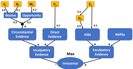
Example 2. Let us consider a simple robbery case. The defendant D is accused of having robbed the victim V . The extended BLAF is shown in Figure 4. Before the crime, D and V met in a bar and had a fight about money that V owed D . V testified that D threatened to get the money one way or another ( V 1 ). D acknowledged the fight, but denied the threat ( D 1 ). While D's testimony still contains a motive for the crime, it is now significantly weaker. This can be reflected in the weights. We could consider a more fine-grained view distinguishing the fight and the threat and add an attack between the contradicting statements, but in order to keep things simple, we refrain from doing so. V testified that he got robbed at 23:30 by a masked person
Figure 4: Extended BLAF for Example 2.
<details>
<summary>Image 4 Details</summary>
### Visual Description
## Diagram: Evidence and Innocence Model
### Overview
The image presents a causal loop diagram illustrating the relationship between various types of evidence (Motive, Opportunity, Direct Evidence, Alibi, Ability) and the concepts of Innocence, Circumstantial Evidence, Incultpatory Evidence, and Exculpatory Evidence. The diagram uses arrows to indicate causal relationships, with "+" signs indicating positive (reinforcing) relationships and the absence of a sign implying a negative (balancing) relationship. Numerical values are associated with some arrows, representing the strength of the causal link.
### Components/Axes
The diagram consists of the following components:
* **Variables:** V1, D1, W1, V2, E1, D2. These are represented by yellow boxes.
* **Concepts:** Motive, Opportunity, Circumstantial Evidence, Direct Evidence, Alibi, Ability, Incultpatory Evidence, Exculpatory Evidence, Innocence, Max. These are represented by blue boxes.
* **Causal Links:** Arrows connecting the variables and concepts, with associated numerical values.
* **Polarity:** "+" signs indicating positive causal relationships.
### Detailed Analysis
The diagram can be divided into two main sections: a left side focusing on evidence leading towards guilt and a right side focusing on evidence leading towards innocence.
**Left Side (Guilt):**
* **Motive:** V1 (0.9) influences Motive. Motive (0.3) and Opportunity (0.3) combine to form Circumstantial Evidence.
* **Opportunity:** D1 (0.1) influences Opportunity. W1 (0.2) influences Opportunity.
* **Circumstantial Evidence:** Positively influences Incultpatory Evidence.
* **Direct Evidence:** V2 (0.2) influences Direct Evidence. Direct Evidence positively influences Incultpatory Evidence.
* **Incultpatory Evidence:** Positively influences Innocence.
**Right Side (Innocence):**
* **Alibi:** E1 (0.3) influences Alibi. D2 (0.9) influences Alibi. Alibi positively influences Exculpatory Evidence.
* **Ability:** Ability positively influences Exculpatory Evidence.
* **Exculpatory Evidence:** Positively influences Innocence.
**Final Stage:**
* **Innocence:** Both Incultpatory Evidence and Exculpatory Evidence positively influence Innocence.
* **Max:** The "Max" label is positioned above the connection between Incultpatory Evidence and Exculpatory Evidence to Innocence.
**Numerical Values (Causal Link Strengths):**
* V1 -> Motive: 0.9
* D1 -> Opportunity: 0.1
* W1 -> Opportunity: 0.2
* V2 -> Direct Evidence: 0.2
* E1 -> Alibi: 0.3
* D2 -> Alibi: 0.9
* Motive + Opportunity -> Circumstantial Evidence: 0.3
* Circumstantial Evidence -> Incultpatory Evidence: +
* Direct Evidence -> Incultpatory Evidence: +
* Alibi -> Exculpatory Evidence: +
* Ability -> Exculpatory Evidence: +
* Incultpatory Evidence -> Innocence: +
* Exculpatory Evidence -> Innocence: +
### Key Observations
* The diagram highlights the interplay between different types of evidence in determining a conclusion of innocence or guilt.
* The strength of the causal links varies significantly. For example, V1 has a strong influence on Motive (0.9), while V2 has a weaker influence on Direct Evidence (0.2).
* The diagram suggests that both incriminating and exonerating evidence contribute to the overall assessment of innocence.
* The "Max" label suggests a point of culmination or maximum impact of the evidence on the final determination of innocence.
### Interpretation
This diagram represents a simplified model of how evidence is evaluated in a legal or investigative context. It demonstrates that establishing innocence or guilt is not a simple linear process but rather a complex interplay of various factors. The diagram suggests that a strong motive (V1) is a significant driver of the perception of guilt, while a strong alibi (D2) is a significant driver of the perception of innocence. The positive signs indicate that increasing the strength of incriminating or exonerating evidence will reinforce the corresponding conclusion. The diagram is a conceptual tool for understanding the dynamics of evidence and its impact on the determination of innocence. The numerical values provide a relative measure of the importance of each factor, but it's important to note that these values are likely subjective and based on assumptions. The diagram does not provide any factual data, but rather a theoretical framework for analyzing evidence.
</details>
and that he recognized the defendant based on his voice and stature ( V 2 ). This can be seen as direct evidence for the crime, but since the accused is of average stature, it should have only a small weight. A waiter working at the bar testified that the defendant left the bar at about 23:00 ( W 1 ). This may have allowed the defendant hypothetically to commit the crime, but he could have went anywhere, so the weight should be again low. The defendant testified that he went to the movie theater and watched a movie that started at 23:15 ( D 2 ). If true, this is a strong alibi and should therefore have a large weight. An employee at the movie theater testified that the defendant is a frequent guest and that he recalled him buying a drink ( E 1 ). However, he did not recall the exact time. So the alibi is somewhat weak and should not have too much weight. We weigh Motive and Opportunity equally with w((Motive , Innocence)) = w((Opportunity , Innocence)) = 0 . 3 . The influence of the belief in motive and opportunity on circumstantial evidence is defined by the collective support constraint that we described above. All evidential edges ( E,A ) that originate from a piece of evidence E are associated with the constraint w (( E,A )) · π ( E ) ≤ π ( A ) . Figure 4 shows the final graph structure and edge weights.
Having defined the structure of the graph and the meaning of the edges, we can start to assign beliefs to pieces of evidence. Again, without making any assumptions about the beliefs, we can only infer that the degree of belief in Innocence is 1. This is shown in the second column of Table 2. To begin with, we assume that the testimonies given by the cinema employee and the waiter of the bar are true ( π ( E 1) = 1 , π ( W 1) = 1 ). The third column of Table 2 shows the consequences of these assumptions. We can see, for example, that the alibi E 1 provides a lower bound for the belief in the exculpatory evidence and thus an upper bound for the beliefs in the inculpatory evidence and the related hypotheses. It seems also safe to assume that the defendant did not lie about his participation in the fight, so we the constraint π ( D 1) = 1 next. The fourth column in Table 2 shows the resulting belief intervals. The new support for motive adds to the support of the circumstantial evidence and the lower bound on the belief in the inculpatory evidence is raised. This lowers the belief in the innocence of the accused slightly. Note again that it also decreases the upper bound on the belief in exculpatory evidence indirectly. Fi-
Table 2: Belief in Innocence and entailment results under additional assumptions for Example 2 (rounded to two digits). Directly constrained beliefs are highlighted in bold.
| A | Basic | W 1 , E 1 | W 1 , E 1 , D 1 | W 1 , E 1 , D 1 , V 2 |
|-------------|---------|-------------|-------------------|-------------------------|
| Innocence | [0, 1] | 0.94 | 0.91 | 0.8 |
| E inc | [0, 1] | [0.06, 0.7] | [0.09, 0.7] | [0.2, 7] |
| E ex | [0, 1] | [0.3, 0.94] | [0.3, 0.91] | [0.3, 0.8] |
| E c | [0, 1] | [0.06, 0.7] | [0.09, 0.7] | [0.09, 0.7] |
| E d | [0, 1] | [0, 0.7] | [0, 0.7] | [0.2, 0.7] |
| Alibi | [0, 1] | [0.3, 0.94] | [0.3, 0.91] | [0.3, 0.8] |
| Ability | [0, 1] | [0, 0.94] | [0, 0.91] | [0, 0.8] |
| Motive | [0, 1] | [0, 1] | [0.1, 1] | [0.1, 1] |
| Opportunity | [0, 1] | [0.2, 1] | [0.2, 1] | [0.2, 1] |
| V 1 | [0, 1] | [0, 1] | [0, 1] | [0, 1] |
| V 2 | [0, 1] | [0, 1] | [0, 1] | 1 |
| D 1 | [0, 1] | [0, 1] | 1 | 1 |
| D 2 | [0, 1] | [0.3, 1] | [0.3, 1] | [0.3, 0.89] |
| W 1 | [0, 1] | 1 | 1 | 1 |
| E 1 | [0, 1] | 1 | 1 | 1 |
nally, let us assume that the defendant does not lie about having recognized the defendant ( π ( V 2) = 1 ) (recall that the uncertainty about the recognition reliability is incorporated in the edge weight). The fifth column in Table 2 shows the new beliefs. We can see that the belief in the defendant's innocence decreases significantly. If we notice that a larger or smaller change is more plausible, we could take account of this by adapting the edge weight. In this way, legal cases can be analyzed in a systematic way and the plausibility of assumptions can be checked on the fly by looking at their ramifications.
In addition to the previously introduced additional categories of meta-hypotheses, another recurring pattern in legal cases are mutually dependent pieces of evidence. One way to model this in our framework, is to define a meta-argument that is influenced by the dependent pieces of evidence. The collective support constraint CS is well suited to capture this relationship accurately. We illustrate this with an example from (Fenton, Neil, and Lagnado 2013, pp.82-84).
Example 3. Let us assume that a person was recorded by two video cameras from different perspectives at a crime scene. If the person is the defendant, the defendant should resemble the person on both images. In the BLAF, we can incorporate the two camera observations as pieces of evidence Camera1 , Camera2 supporting a meta-hypothesis Camera that says that the defendant was at the crime scene because of camera evidence. Note that if we use the SE constraint for the evidential edges from Camera1 , Camera2 , each of the two cameras would independently determine a lower bound for Camera which seems to strong in this example. Instead, we can use the CS constraint that we already used to capture the relationship between opportunity and motive. In this example, the CS constraint becomes w((Camera1 , Camera)) · π (Camera1) + w((Camera2 , Camera)) · π (Camera2) ≤
π (Camera) , where w((Camera1 , Camera)) + w((Camera2 , Camera)) ≤ 1 . For example both camera weights could be set to w((Camera1 , Camera)) = w((Camera2 , Camera)) = 0 . 5 to give equal relevance to both. Then, if the person resembles the defendant only from one perspective, say we have π (Camera1) = 1 and π (Camera2) = 0 , the induced lower bound on the belief in Camera will be only 0 . 5 . Only if the belief in both cameras is larger than 0 . 5 , the lower bound can be larger than 0 . 5 . For example, if we have π (Camera1) = 0 . 7 and π (Camera2) = 0 . 9 , the induced lower bound is 0 . 8 .
## 5 Automated Explanation Generation
As we already illustrated at the end of Section 3, the structure of our framework allows generating explanations for decisions automatically. In general, explaining the metahypotheses Innocence , E inc and E ex is easier than explaining the beliefs in other arguments because of their restricted form.
Note first that the only direct neighbors of Innocence are E inc and E ex and we know that E inc is an attacker and E ex is a supporter. Therefore, we can basically distinguish three cases that we already described at the end of Section 3.
1. B (E inc ) ≤ T and B (E ex ) ≤ 0 . 5 : The defendant is found innocent due to lack of evidence.
2. B (E ex ) > 0 . 5 : the defendant is found innocent because the exculpatory evidence is more plausible than the inculpatory evidence.
3. B (E inc ) > T : the defendant is found guilty because of the inculpatory evidence.
Here, T is a threshold that should usually be chosen from the open interval (0 . 5 , 1) . 0 . 5 is sometimes regarded as the acceptance threshold, but in a legal setting, it may be more appropriate to choose a larger threshold like T = 0 . 75 .
After having received a high-level explanation of the verdict, the user may be interested in more details and ask for reasons that explain the plausibility of inculpatory or exculpatory evidence. Explaining E inc and E ex is more complicated already because we have an unknown number of neighbors in the graph now. However, the only neighbors can be supporters (parents) and Innocence (child). By Definition 1, item 4, their meaning is encoded by the SE -constraint. Assuming that the user did not add additional constraints about the relationships between E inc , E ex and Innocence , we can again define some simple rules. If additional constraints on E inc and E ex are desirable, these rules may need to be refined, of course. Otherwise, we can distinguish two cases. If the user asks for an explanation for the lower belief, we can reason as follows: a non-trivial lower bound ( > 0 ) can only result from a supporter with non-trivial lower bound. So in this case, we can go through the supporters, collect those supporters that induce the maximum lower bound and report them as an explanation.
The user may also ask for an explanation for the upper belief. A non-trivial upper bound ( < 1 ) can only result from a non-trivial bound on the belief in Innocence . Let us assume that we want to explain a non-trivial upper bound on
E inc . From the IE -constraint in Definition 1, item 4, we can see that this must be caused by a non-trivial lower bound on Innocence . This lower bound, in turn, must be caused by a non-trivial lower bound on E ex by our assumptions. We could now report the lower bound on E ex as an explanation. A more meaningful explanation would be obtained by also explaining the lower bound on E ex . This can be done as explained before by looking at the supporters of E ex . A non-trivial upper bound on E ex can be explained in a symmetrical manner.
Generating automatic explanations for the remaining subhypotheses and pieces of evidence is most challenging, but can be done as long as we can make assumptions about the constraints that are involved. For example, often the SE -constraint gives a natural meaning to support edges and the weighted Coherence constraint gives a natural meaning to attack edges. Intuitively, they cause a lower/upper bound on the belief in an argument based on their own lower belief. If these are the only constraints that are employed, explanations for lower bounds can again be generated by collecting the supporters that induce the largest lower bound. For explaining the upper bound, we now have to consider two factors. The first factor are attackers with a non-trivial lower bound. The second factor are other arguments that are supported and have a non-trivial upper bound (then a too large belief in the supporting argument would cause an inconsistency). Therefore, we do not only collect the attacking arguments that induce the largest lower bound, but we also collect supported arguments. We can order the supported arguments by their upper belief multiplied by the weight of the support edge. If the smallest upper bound from the supported arguments is U and the largest lower bound from the attacking arguments is L , we report the collected supported arguments as an explanation if 1 -U > L , the collected attacking arguments as an explanation if 1 -U < L or both if it happens that 1 -U = L .
For additional constraints, we may have to refine these rules again. One important constraint that we discussed is the CS -constraint. In this case, we have to to treat the supporters involved in this constraint differently since they all contribute to the induced lower bound. When collecting supporters for explaining lower bounds (the supporters are parents), supporting edges that belong to one CS -constraint have to be considered jointly and not independently. If they induce a lower bound that is larger than all lower bounds caused by an SE -constraint, they can be reported collectively as an explanation. When collecting supporters for explaining upper bounds (the supporters are children), the reasoning becomes more complicated because there can be various interactions between the beliefs in the involved arguments. We leave an analysis of this case and more general cases for future work.
## 6 Related Work
Our legal reasoning framework allows explicit formalization of uncertainty in legal decision making. Other knowledge representation and reasoning formalisms have been applied for this purpose. Studies of different game-theoretical tools can be found in (Prakken and Sartor 1996; Riveret et al.
2007; Roth et al. 2007). (Dung and Thang 2010) proposed a probabilistic argumentation framework where the beliefs of different jurors are represented by individual probability spaces. Intuitively, the jurors weigh the evidence and decisions can be made based on criteria like majority voting or belief thresholds. One particularly popular approach for probabilistic legal reasoning are Bayesian networks. (Fenton, Neil, and Lagnado 2013) provide a set of idioms used for the construction of Bayesian networks based on legal argument patterns and apply and discuss their framework for a specific case in (Fenton et al. 2019). (Timmer et al. 2017) developed an algorithm to extract argumentative information from a Bayesian network with an intermediate structure, a support graph and analyze their approach in a legal case study. (Vlek et al. 2016) propose a method to model different scenarios about crimes with Bayesian networks using scenario scheme idioms and to extract information about the scenario and the quality of the scenario.
Determining the weights and beliefs for the edges and items of evidence poses a problem for our framework as well as for other symbolic approaches. For some items of evidence the weights as well as the probabilities can be elicited based on statistical analysis and forensic evidence (Kwan et al. 2011; Fenton and Neil 2012; Zhang and Thai 2016). To test the robustness of Bayesian networks with respect to minor changes in subjective beliefs, (Fenton, Neil, and Lagnado 2013) propose to apply sensitivity analysis on the nodes in question. In our framework, the impact of subjective beliefs can be analysed in a similar manner, by altering the beliefs which are associated with the evidence or the weights associated with the edges. The automated explanation generation outlined in Section 5 can then provide information about the influence that differing beliefs have on hypotheses and subhypotheses in the framework. With this the perspective of different agents can be modeled, for example the defense and prosecution perspectives. The clear structure of argumentation frameworks is well suited for generating explanations automatically and related explanation ideas have been considered recently in (Cocarascu, Rago, and Toni 2019; ˇ Cyras et al. 2019; Zeng et al. 2018), for example.
In Bayesian networks, inconsistency is usually not an issue because of the way how they are defined. In contrast, in our framework, inconsistencies can easily occur. For example, if a forensic expert judges both the accuracy of an alibi and the relevance of a direct piece of evidence with 1 , our constraints become inconsistent. While this may be inconvenient, this inconsistency is arguably desirable. This is because the modeling assumptions are inconsistent and this should be recognized and reported by the system. If automated merging of the inconsistent beliefs is desirable, this can be achieved by different tools. One possibility is to apply inconsistency measures for probabilistic logics in order to evaluate the severity of conflicts (De Bona and Finger 2015; Potyka 2014; Thimm 2013). In order to determine the sources of the inconsistency and their impact, Shapley values can be applied (Hunter and Konieczny 2010). Alternatively, we could replace our exact probabilistic reasoning algorithms with inconsistency-tolerant reasoning approaches that resolve inconsistencies by minimizing conflicts (Adamcik 2014; Mui˜ no 2011; Potyka and Thimm 2015) or based on priorities (Potyka 2015). This would be more convenient for the knowledge engineer, but the resulting meaning of the probabilities becomes less clear.
## 7 Conclusions and Future Work
We proposed a probabilistic abstract argumentation framework for automated reasoning in law based on probabilistic epistemic argumentation (Hunter and Thimm 2016; Hunter, Polberg, and Thimm 2018). Our framework is best suited for merging beliefs in pieces of evidence and sub-hypotheses. Computing an initial degree of belief for particular pieces of evidence based on forensic evidence can often be better accomplished by applying Bayesian networks or a conventional statistical analysis. Our framework can then be applied on top in order to merge the different beliefs in pieces of evidence and subhypotheses in a transparent and explainable way. In particular, point probabilities are not required, but imprecise probabilities in the form of belief intervals are supported as well.
It is also interesting to note that the worst-case runtime of our framework is polynomial (Potyka 2019). Bayesian networks also have polynomial runtime guarantees in some special cases, for example, when the Bayesian network structure is a polytree (i.e., it does not contain cycles when ignoring the direction of the edges). The polynomial runtime in probabilistic epistemic argumentation is guaranteed by restricting to a fragment of the full language. This fragment is sufficient for many cases and is all that we used in this work. However, sometimes it may be necessary to extend the language. For example, instead of talking only about the probabilities of single pieces of evidence and subhypotheses, we may want to talk about the probabilities of logical combinations. Similarly, one may want to merge beliefs not only in a linear, but in a non-linear way. Both extensions are difficult to deal with, in general. However, it seems worthwhile to study such cases in more detail in order to identify some other tractable special cases.
Another interesting aspect for future work is extending the automated support tools for designing and querying our legal argumentation frameworks. As explained in Section 5, the basic framework can be explained well automatically. However, when beliefs are merged in more complicated ways like by the collective support constraint, a deeper analysis is required. We will study explanation generation for collective support and other interesting merging patterns in more detail in future work. For the design of the framework, it may also be helpful to generate explanations for the sources of inconsistency. As explained in the related work section, a combination of inconsistency measures for probabilistic logics and Shapley values seems like a promising approach that we will study. It is also interesting to apply different approaches for inconsistency-tolerant reasoning in order to avoid inconsistencies altogether. However, while these approaches usually can give some meaningful analytical guarantees, it is important to study empirically if these guarantees are sufficient in order to guarantee meaningful results in legal or other applications.
Adamcik, M. 2014. Collective reasoning under uncertainty and inconsistency . Ph.D. Dissertation, Manchester Institute for Mathematical Sciences, The University of Manchester.
Bench-Capon, T., and Sartor, G. 2003. A model of legal reasoning with cases incorporating theories and values. Artificial Intelligence 150(1-2):97-143.
Cocarascu, O.; Rago, A.; and Toni, F. 2019. Extracting dialogical explanations for review aggregations with argumentative dialogical agents. In International Conference on Autonomous Agents and Multiagent Systems (AAMAS) , 12611269. International Foundation for Autonomous Agents and Multiagent Systems.
ˇ Cyras, K.; Letsios, D.; Misener, R.; and Toni, F. 2019. Argumentation for explainable scheduling. In AAAI Conference on Artificial Intelligence (AAAI) , volume 33, 2752-2759.
De Bona, G., and Finger, M. 2015. Measuring inconsistency in probabilistic logic: rationality postulates and dutch book interpretation. Artificial Intelligence 227:140-164.
Dung, P. M., and Thang, P. M. 2010. Towards (probabilistic) argumentation for jury-based dispute resolution. International Conference on Computational Models of Argument (COMMA) 216:171-182.
Fenton, N., and Neil, M. 2012. Risk assessment and decision analysis with Bayesian networks . Crc Press.
Fenton, N.; Neil, M.; Yet, B.; and Lagnado, D. 2019. Analyzing the simonshaven case using bayesian networks. Topics in cognitive science .
Fenton, N.; Neil, M.; and Lagnado, D. A. 2013. A general structure for legal arguments about evidence using bayesian networks. Cognitive science 37(1):61-102.
Hanson, J.; Hanson, K.; and Hart, M. 2014. Game theory and the law. In Game Theory and Business Applications . Springer. 233-263.
Hunter, A., and Konieczny, S. 2010. On the measure of conflicts: Shapley inconsistency values. Artificial Intelligence 174(14):1007-1026.
Hunter, A., and Thimm, M. 2016. On partial information and contradictions in probabilistic abstract argumentation. In International Conference on Principles of Knowledge Representation and Reasoning (KR) , 53-62. AAAI Press.
Hunter, A.; Polberg, S.; and Thimm, M. 2018. Epistemic graphs for representing and reasoning with positive and negative influences of arguments. ArXiv .
Hunter, A. 2013. A probabilistic approach to modelling uncertain logical arguments. International Journal of Approximate Reasoning 54(1):47-81.
Kwan, M.; Overill, R.; Chow, K.-P.; Tse, H.; Law, F.; and Lai, P. 2011. Sensitivity analysis of bayesian networks used in forensic investigations. In International Conference on Digital Forensics (IFIP) , 231-243. Springer.
McCarty, L. T. 1995. An implementation of eisner v. macomber. In International Conference on Artificial Intelligence and Law (ICAIL) , volume 95, 276-286.
Mui˜ no, D. P. 2011. Measuring and repairing inconsistency in probabilistic knowledge bases. International Journal of Approximate Reasoning 52(6):828-840.
Potyka, N., and Thimm, M. 2015. Probabilistic reasoning with inconsistent beliefs using inconsistency measures. In International Joint Conference on Artificial Intelligence (IJCAI) .
Potyka, N. 2014. Linear programs for measuring inconsistency in probabilistic logics. In International Conference on Principles of Knowledge Representation and Reasoning (KR) .
Potyka, N. 2015. Reasoning over linear probabilistic knowledge bases with priorities. In International Conference on Scalable Uncertainty Management (SUM) , 121136. Springer.
Potyka, N. 2019. A polynomial-time fragment of epistemic probabilistic argumentation. International Journal of Approximate Reasoning 115(1):265-289.
Prakken, H., and Sartor, G. 1996. A dialectical model of assessing conflicting arguments in legal reasoning. In Logical models of legal argumentation . Springer. 175-211.
Prakken, H.; Wyner, A.; Bench-Capon, T.; and Atkinson, K. 2013. A formalization of argumentation schemes for legal case-based reasoning in aspic+. Journal of Logic and Computation 25(5):1141-1166.
Riveret, R.; Rotolo, A.; Sartor, G.; Bram, R.; and Prakken, H. 2007. Success chances in argument games: a probabilistic approach to legal disputes. Conference on Legal Knowledge and Information Systems (JURIX) .
Roth, B.; Riveret, R.; Rotolo, A.; and Governatori, G. 2007. Strategic argumentation: a game theoretical investigation. In International Conference on Artificial Intelligence and Law , 81-90. ACM.
Thimm, M. 2012. A probabilistic semantics for abstract argumentation. In European Conference on Artificial Intelligence (ECAI) , volume 12, 750-755.
Thimm, M. 2013. Inconsistency measures for probabilistic logics. Artificial Intelligence 197:1-24.
Timmer, S. T.; Meyer, J.-J. C.; Prakken, H.; Renooij, S.; and Verheij, B. 2017. A two-phase method for extracting explanatory arguments from bayesian networks. International Journal of Approximate Reasoning 80:475-494.
Vlek, C. S.; Prakken, H.; Renooij, S.; and Verheij, B. 2016. A method for explaining bayesian networks for legal evidence with scenarios. Artificial Intelligence and Law 24(3):285-324.
Zeng, Z.; Fan, X.; Miao, C.; Leung, C.; Jih, C. J.; and Soon, O. Y. 2018. Context-based and explainable decision making with argumentation. In International Conference on Autonomous Agents and Multiagent Systems (AAMAS) , 11141122. International Foundation for Autonomous Agents and Multiagent Systems.
Zhang, G., and Thai, V. V. 2016. Expert elicitation and bayesian network modeling for shipping accidents: A literature review. Safety science 87:53-62.