## FastSecAgg: Scalable Secure Aggregation for Privacy-Preserving Federated Learning
Swanand Kadhe, Nived Rajaraman, O. Ozan Koyluoglu, and Kannan Ramchandran
University of California Berkeley
Department of Electrical Engineering and Computer Sciences f swanand.kadhe,nived,ozan.koyluoglu,kannanr g @berkeley.edu
## ABSTRACT
Recent attacks on federated learning demonstrate that keeping the training data on clients' devices does not provide sufficient privacy, as the model parameters shared by clients can leak information about their training data. A secure aggregation protocol enables the server to aggregate clients' models in a privacy-preserving manner. However, existing secure aggregation protocols incur high computation/communication costs, especially when the number of model parameters is larger than the number of clients participating in an iteration - a typical scenario in federated learning.
subset of clients, and sends them the current global model. Each client runs several steps of mini-batch stochastic gradient descent, and communicates its model update-the difference between the local model and the received global model-to the server. The server aggregates the model updates from the clients to obtain an improved global model, and moves to the next iteration.
In this paper, we propose a secure aggregation protocol, FastSecAgg, that is efficient in terms of computation and communication, and robust to client dropouts. The main building block of FastSecAgg is a novel multi-secret sharing scheme, FastShare, based on the Fast Fourier Transform (FFT), which may be of independent interest. FastShare is information-theoretically secure, and achieves a trade-off between the number of secrets, privacy threshold, and dropout tolerance. Riding on the capabilities of FastShare, we prove that FastSecAgg is (i) secure against the server colluding with any subset of some constant fraction (e.g. 10%) of the clients in the honest-but-curious setting; and (ii) tolerates dropouts of a random subset of some constant fraction (e.g. 10%) of the clients. FastSecAgg achieves significantly smaller computation cost than existing schemes while achieving the same (orderwise) communication cost. In addition, it guarantees security against adaptive adversaries, which can perform client corruptions dynamically during the execution of the protocol.
## CCS CONCEPTS
· Security and privacy ! Privacy-preserving protocols;
## KEYWORDS
secret sharing, secure aggregation, federated learning, machine learning, data sketching, privacy-preserving protocols
## 1 INTRODUCTION
Federated Learning (FL) is a distributed learning paradigm that enables a large number of clients to coordinate with a central server to learn a shared model while keeping all the training data on clients' devices. In particular, training a neural net in a federated manner is an iterative process. In each iteration of FL, the server selects a
A shorter version of this paper has been accepted in ICML Workshop on Federated Learning for User Privacy and Data Confidentiality, July 2020, and CCS Workshop on Privacy-Preserving Machine Learning in Practice, November 2020.
Secure aggregation protocols can be used to provide strong privacy guarantees in FL. At a high level, secure aggregation is a secure multi-party computation (MPC) protocol that enables the server to compute the sum of clients' model updates without learning any information about any client's individual update [9]. Secure aggregation can be efficiently composed with differential privacy to further enhance privacy guarantees [9, 22, 45].
FL ensures that every client keeps their local data on their own device, and sends only model updates that are functions of their dataset. Even though any update cannot contain more information than the client's local dataset, the updates may still leak significant information making them vulnerable to inference and inversion attacks [17, 19, 33, 40]. Even well-generalized deep models such as DenseNet can leak a significant amount of information about their training data [33]. In fact, certain neural networks (e.g., generative text models) trained on sensitive data (e.g., private text messages) can memorize the training data [13].
The secure aggregation problem for securely computing the summation has received significant research attention in the past few years, see [22] for a survey. However, the FL setup presents unique challenges for a secure aggregation protocol [8, 28]:
- (1) Massive scale: Up to 10,000 users can be selected to participate in an iteration.
- (3) Dropouts: Clients are mobile devices which can drop out at any point. The percentage of dropouts can go up to 10%.
- (2) Communication costs: Model updates can be high-dimensional vectors, e.g., the ResNet model consists of hundreds of millions of parameters [23].
- (4) Privacy: It is crucial to provide strongest possible privacy guarantees since malicious servers can launch powerful attacks by using sybils [14], wherein the adversary simulates a large number of fake client devices [18].
Due to these challenges, existing secure aggregation protocols for FL [3, 9, 43, 45, 47] either incur heavy computation and communication costs or provide only weaker forms of privacy guarantees, which limits their scalability (see Table 1).
Secret sharing [2] is an elegant primitive that is used as a building block in a large number of secure summation (and in general secure MPC) protocols, see, e.g., [15, 22]. Secret sharing based secure aggregation protocols are often more efficient than other approaches such as homomorphic encryption and Yao's garbled
Table 1: Comparison of the proposed FastSecAgg with SecAgg [9], TurboAgg [43], and SecAgg+ [3]. Here N is the total number of clients and L is the length of model updates (i.e., client inputs). An adaptive adversary can choose which clients to corrupt during the protocol execution, whereas the corruptions happen before the protocol execution starts for a non-adaptive adversary. Worst-case (resp. average-case) dropout guarantee ensures that any (resp. a random) subset of clients of a bounded size may drop out without affecting the correctness and security. TurboAgg requires at least log N rounds, which increases the overheads. The protocols in [45, 47] assume a trusted third party for key distribution (see Sec. 5.3 for details).
| Protocol | Computation (Server) | Communication (Server) | Computation (Client) | Communication (Client) | Adversary | Dropouts |
|---------------|------------------------------------------|------------------------------|-----------------------------------------|--------------------------|--------------|--------------|
| SecAgg [9] | O LN 2 | O LN + N 2 | O LN + N 2 | O' L + N ' | Adaptive | Worst-case |
| TurboAgg [43] | O L log N log 2 log N | O' LN log N ' | O L log N log 2 log N | O' L log N ' | Non-adaptive | Average-case |
| SecAgg+ [3] | O LN log N + N log 2 N | O' LN + N log N ' | O L log N + log 2 N | O' L + log N ' | Non-adaptive | Average-case |
| FastSecAgg | O' L log N ' | O LN + N 2 | O' L log N ' | O' L + N ' | Adaptive | Average-case |
circuits [1, 11, 22]. However, na¨ ıvely using the popular Shamir's secret sharing scheme [39] for aggregating lengthL updates from N clients incurs O LN 2 communication and computation cost, which is intractable at the envisioned scale of FL.
Using FastShare as a building block, we propose FastSecAgg - a scalable secure aggregation protocol for FL that has low computation and communication costs and strong privacy guarantees (see Table 1 for a comparison of costs). FastSecAgg achieves low costs by riding on the capabilities of FastShare and leveraging the following unique attribute of FL. Privacy breaches in FL are inflicted by malicious/adversarial actors (e.g., a server using sybils), requiring worst-case guarantees; whereas dropouts occur due to non-adversarial/natural causes (e.g., system dynamics and wireless outages) [8], making statistical or average-case guarantees sufficient. FastShare achieves O' N log N ' computation cost by relaxing the dropout constraint from worst-case to random.
In this paper, we propose FastShare-a novel secret sharing scheme based on a finite-field version of the Fast Fourier Transform (FFT)-that is designed to leverage the FL setup. FastShare is a multi-secret sharing scheme, which can simultaneously share S secrets to N clients such that (i) it is information-theoretically secure against a collusion of any subset of some constant fraction (e.g. 10%) of the clients; and (ii) with overwhelming probability, it is able to recover the secrets with O' N log N ' complexity even if a random subset of some constant fraction (e.g. 10%) of the clients drop out. In general, FashShare can achieve a trade-off between the security and dropout parameters (see Theorem 3.3); thresholds of 10% are chosen to be well-suited in the FL setup. We note that a larger number of arbitrary (or even adversarial) dropouts does not affect security, and may only result in a failure to recover the secrets (i.e, affects only correctness). FastShare uses ideas from sparsegraph codes [27, 29, 38] and crucially exploits insights derived from a spectral view of codes [6, 34], which enables us to prove strong privacy guarantees.
For N clients, each having a lengthL update vector, FastSecAgg requires O' L log N ' computation and O LN + N 2 communication at the server, and O' L log N ' computation and O' L + N ' communication per client. We compare the costs and setups with existing protocols in Table 1 (see Sec. 5.3 for details). We point out that the computation cost at the server was observed to be the key barrier to scalability in [8, 9]. FastSecAgg significantly reduces the computation cost at the server as compared to prior works. When the length of model updates L is larger than the number of clients N , FastSecAgg achieves the same (order-wise) communication cost as the prior works. We note that, in typical FL applications, the number of model parameters ' L ' is in millions, whereas the number of clients ' N ' is up to tens of thousands [8, 32]. In addition, FastSecAgg guarantees security against an adaptive adversary, which can corrupt clients adaptively during the execution of the protocol. This is in contrast with the protocols in [3, 43], which are secure only against non-adaptive (or static) adversaries, wherein client corruptions happen before the protocol executions begins.
We note that, although FastShare secret sharing scheme is inspired from the federated learning setup, it may be of independent interest. In fact, FastShare is a cryptographic primitive that can be used for secure aggregation (and secure multi-party computation in general) in wide applications including smart meters [26], medical data collection [12], and syndromic surveillance [46].
## 2 PROBLEM SETUP AND PRELIMINARIES
## 2.1 Federated Learning
We consider the setup in which a fixed set of M clients, each having their local dataset, coordinate with the server to jointly train a model. The i -th client's data is sampled from a distribution D i . The federated learning problem can be formalized as minimizing a sum of stochastic functions defined as
<!-- formula-not-decoded -->
where ' i ' w ' = E ζ D i » ' i ' w ; ζ '… is the expected loss of the prediction on the i -th client's data made with model parameters w .
Federated Averaging (FedAvg) is a synchronous update scheme that proceeds in rounds of communication [32]. At the beginning of each round (called iteration), the server selects a subset C of N clients (for some N M ). Each of these clients i 2 C copies the current model parameters w t i ; 0 = w t , and performs T steps of (minibatch) stochastic gradient descent steps to obtain its local model w t i ; T ; each local step k is of the form w t i ; k w t i ; k 1 η l д t i ; k 1 , where д t i ; k 1 is an unbiased stochastic gradient of ' i at w t i ; k 1 ,
and η l is the local step-size. 1 Then, each client i 2 C sends their update as ∆ w t i = w t i ; L w t . At the server, the clients' updates ∆ w t i are aggregated to form the new server model as w t + 1 = w t + 1 j C j ˝ i 2C ∆ w t i .
Our focus is on one iteration of FedAvg and we omit the explicit dependence on the iteration t hereafter. We assume that each client potentially compresses and suitably quantizes their model update ∆ w t i 2 R d to obtain u i 2 Z L R , where L d . Our goal is to design a protocol that enables the server to securely compute ˝ i 2C u i . We describe the threat model and the objectives in the next section.
## 2.2 Threat Model
Federated learning can be considered as a multi-party computation consisting of N parties (i.e., the clients), each having their own private dataset, and an aggregator (i.e., the server), with the goal of learning a model using all of the datasets.
Honest-but-curious model: The parties honestly follow the protocol, but attempt to learn about the model updates from other parties by using the messages exchanged during the execution of the protocol. The honest-but-curious (aka semi-honest) adversarial model is commonly used in the field of secure MPC, including prior works on secure federated learning [9, 43, 45].
Colluding parties: In every iteration of federated averaging, the server first samples a set C of clients. The server may collude with any set of up to T clients from C . The server can view the internal state and all the messages received/sent by the clients with whom it colludes. We refer to the internal state along with the messages received/sent by colluding parties (including the server) as their joint view . (see Sec. 5.1 for details)
Dropouts: Arandom subset of up to D clients may drop out at any point of time during the execution of secure aggregation.
Objective: Our objective is to design a protocol to securely aggregate clients' model updates such that the joint view of the server and any set of up to T clients must not leak any information about the other clients' model updates, besides what can be inferred from the output of the summation. In addition, even if a random set of up to D clients drop out during an iteration, the server with high probability should be able to compute the sum of model updates (of the surviving clients) while maintaining the privacy. We refer to T as the privacy threshold and D as the dropout tolerance .
## 2.3 Cryptographic Primitives
2.3.1 Key Agreement. A key agreement protocol consists of three algorithms (KA.param, KA.gen, KA.agree). Given a security parameter λ , the parameter generation algorithm pp KA.param ' λ ' generates some public parameters, over which the protocol will be parameterized. The key generation algorithm allows a client i to generate a private-public key pair ' pk i ; sk i ' KA.gen ' pp ' . The key agreement procedure allows clients i and j to obtain a private shared key k i ; j KA.agree ' sk i ; pk j ' . Correctness requires that, for any key pairs generated by clients i and j
1 In practice, clients can make multiple training passes (called epochs) over its local dataset with a given step size. Further, typically client datasets are of different size, and the server takes a weighted average with weight of a client proportional to the size of its dataset. See [32] for details.
(using KA.gen with the same parameters pp ), KA.agree ' sk i ; pk j ' = KA.agree ' sk j ; pk i ' . Security requires that there exists a simulator Sim KA, which takes as input an output key sampled uniformly at random and the public key of the other client, and simulates the messages of the key agreement execution such that the simulated messages are computationally indistinguishable from the protocol transcript.
2.3.2 Authenticated Encryption. An authenticated encryption allows two parties to communicate with data confidentially and data integrity. It consists of an encryption algorithm AE.enc that takes as input a key and a message and outputs a ciphertext, and a decryption algorithm AE.dec that takes as input a ciphertext and a key and outputs the original plaintext, or a special error symbol ? . For correctness, we require that for all keys k i 2 f 0 ; 1 g λ and all messages m , AE.dec '' k i ; AE.enc ' k i ; m '' = m . For security, we require semantic security under a chosen plaintext attack (INDCPA) and ciphertext integrity (IND-CTXT) [4].
## 3 FASTSHARE: FFT BASED SECRET SHARING
In this section, we present a novel, computationally efficient multisecret sharing scheme FastShare which forms the core of our proposed secure aggregation protocol FastSecAgg (described in the next section).
A multi-secret sharing scheme splits a set of secrets into shares (with one share per client) such that coalitions of clients up to certain size have no information on the secrets, and a random 2 set of clients of large enough size can jointly reconstruct the secrets from their shares. In particular, we consider information-theoretic (perfect) security. A secret sharing scheme is said to be linear if any linear combination of valid share-vectors result in a valid share-vector of the linear combination applied to the respective secret-vectors. We summarize this in the following definition.
Definition 3.1 (Multi-secret Sharing). Let F q be a finite field, and let S , T , D and N be positive integers such that S + T + D < N q . A linear multi-secret sharing scheme over F q consists of two algorithms Share and Recon. The sharing algorithm f' i ; » s … i 'g i 2C Share ' s ; C' is a probabilistic algorithm that takes as input a set of secrets s 2 F S q and a set C of N clients (client-IDs), and produces a set of N shares, each in F q , where share » s … i is assigned to client i in C . For a set D C , the reconstruction algorithm f s ; ?g Recon f' i ; » s … i 'g i 2CnD takes as input the shares corresponding to C n D , and outputs either a set of S field elements s or a special symbol ? . The scheme should satisfy the following requirements.
- (1) T -Privacy: For all s ; s 0 2 F S q and every P C of size at most T , the shares of s and s 0 restricted to P are identically distributed.
- (2) D -Dropout-Resilience: For every s 2 F S q and any random set D C of size at most D , Recon f' i ; » s … i 'g i 2CnD = s with probability at least 1 poly ' N ' .
2 Secret sharing [2] and multi-secret sharing [7, 16] schemes conventionally consider worst-case dropouts. We consider random dropouts to exploit the FL setup.
<details>
<summary>Image 1 Details</summary>
### Visual Description
## Diagram: Secret Sharing Scheme using DFT and Peeling Decoder
### Overview
The image illustrates a secret sharing scheme using Discrete Fourier Transform (DFT) and a Peeling Decoder. The scheme involves encoding a secret with random masks using DFT, distributing shares, and then reconstructing the secret using a Peeling Decoder and Inverse Discrete Fourier Transform (IDFT).
### Components/Axes
The diagram consists of the following components:
* **DFT Block:** A rounded rectangle labeled "DFT".
* **IDFT Block:** A rounded rectangle labeled "IDFT".
* **Peeling Decoder Block:** A rounded rectangle labeled "Peeling Decoder".
* **Input/Output Variables:**
* *x*: Represents the secret combined with random masks and careful zero padding.
* *X*: Represents the shares generated by the DFT.
* *X<sub>v</sub>*: Represents a random subset of shares.
* **Arrows:** Red arrows indicating the flow of data.
* **Text Labels:**
* "Secret + random masks with careful zero padding" near the input *x* to the DFT.
* "Shares" near the output *X* of the DFT.
* "Random subset of shares" near the input *X<sub>v</sub>* to the Peeling Decoder.
* "All shares" near the input *X* to the IDFT.
* "Secret + random masks" near the output *x* of the IDFT.
### Detailed Analysis
The diagram can be divided into two main stages: encoding and decoding.
**Encoding (Top Row):**
1. The secret *x*, combined with random masks and careful zero padding, is input to the DFT block.
2. The DFT block transforms the input *x* into *X*, which represents the shares.
3. The shares *X* are distributed.
**Decoding (Bottom Row):**
1. A random subset of shares, *X<sub>v</sub>*, is input to the Peeling Decoder block.
2. The Peeling Decoder processes the subset of shares and outputs *X*, representing all shares.
3. All shares *X* are input to the IDFT block.
4. The IDFT block transforms the shares back into *x*, which represents the reconstructed secret combined with random masks.
### Key Observations
* The DFT is used to encode the secret into shares.
* A subset of shares is sufficient for the Peeling Decoder to reconstruct all shares.
* The IDFT is used to reconstruct the secret from the shares.
* Random masks are used to protect the secret during encoding and decoding.
### Interpretation
The diagram illustrates a secret sharing scheme that leverages the properties of DFT and a Peeling Decoder. The DFT allows for the distribution of the secret into multiple shares, while the Peeling Decoder enables the reconstruction of all shares from a subset. This scheme provides a level of security, as the secret cannot be recovered without a sufficient number of shares. The use of random masks further enhances the security by obscuring the secret during encoding and decoding. The scheme is robust, as it can tolerate the loss of some shares without compromising the ability to reconstruct the secret.
</details>
of shares
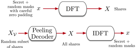
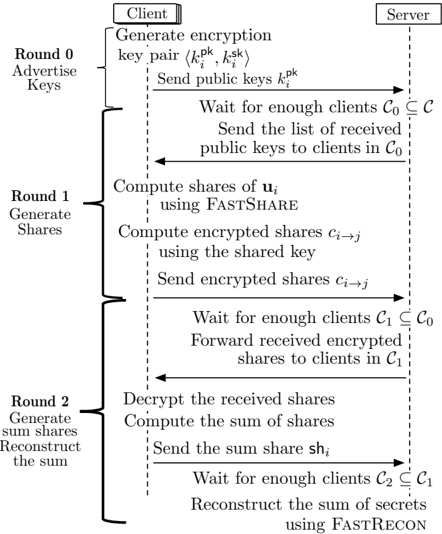
Figure 1: FastShare to generate shares, and FastRecon to recover the secrets from a subset of shares.
- (3) Linearity: If f' i ; » s 1 … i 'g i 2C and f' i ; » s 2 … i 'g i 2C are sharings of s 1 and s 2, then f' i ; a » s 1 … i + b » s 2 … i 'g i 2C is a sharing of a s 1 + b s 2 for any a ; b 2 F q .
Next, we describe FastShare which can achieve a trade-off between S , T , and D for a given N . We begin with setting up the necessary notation. FastShare leverages the finite-field Fourier transform and Chinese Remainder Theorem. Towards this end, let f n 0 ; n 1 g be co-prime positive integers of the same order, such that n 0 n 1 divides ' q 1 ' . Without loss of generality, assume that n 0 < n 1. E.g., n 0 = 10, n 1 = 13, and q = 131. We consider N of the form N = n 0 n 1, and choose the field size q as a power of a prime such that N divides q 1. By the co-primeness of n 0 and n 1, applying the Chinese Remainder Theorem, any number j 2 f 0 ; ; n 1 g can be uniquely represented in a 2-dimensional (2D) grid as a tuple ' a ; b ' where a = j mod n 0 and b = j mod n 1.
## 3.1 FastShare to Generate Shares
The sharing algorithm f' i ; » s … i 'g i 2C FastShare ' s ; C' is a probabilistic algorithm that takes as input a set of secrets s 2 F S q , and a set C of N clients (client-IDs), and produces a set of N shares, each in F q , where share » s … i is assigned to client i . At a high level, FastShare consists of two stages. First, it constructs a lengthN 'signal' consisting of the secrets and random masks with zeros placed at judiciously chosen locations. Second, it takes the fast Fourier transform of the signal to generate the shares (see Fig. 1). The shares can be considered as the 'spectrum' of the signal constructed in the first stage.
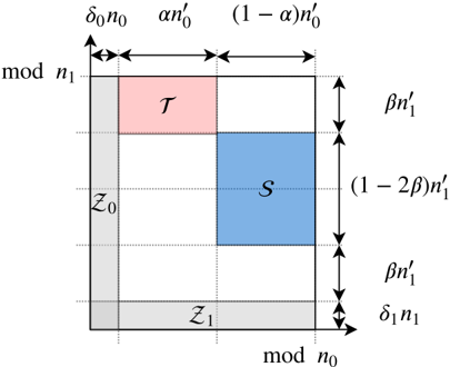
In particular, the 'signal' is constructed as follows. Given fractions δ 0 ; δ 1 ; α 2 ' 0 ; 1 ' and β 2 ' 0 ; 1 2 ' , we define the sets of tuples Z 0, Z 1, S , and T using the grid representation as depicted in Fig. 2. We give the formal definitions below. Here, we round any real number to the largest integer no larger than it, i.e., round x to b x c , and omit the floor sign for the sake of brevity.
<!-- formula-not-decoded -->
<!-- formula-not-decoded -->
S
=
f'
a
δ
;
b
n
'
:
δ
+
β
n
'
+
δ
α
'
'
n
δ
b
'
n
δ
a
n
+
n
'
β
;
''
δ
'
n
g
;
(4)
<!-- formula-not-decoded -->
We place zeros at indices in Z 0 and Z 1, and secrets at indices S . Each of the remaining indices is assigned a uniform random mask from F q (independent of other masks and the secrets). We use T
Figure 2: Indices assigned to a grid using the Chinese remainder theorem, and sets Z 0 , Z 1 , S , and T . Here, we define n 0 i = ' 1 δ i ' n i for i 2 f 0 ; 1 g . Set S is used for secrets, and sets Z 0 and Z 1 are used for zeros, and the remaining locations are used for random masks. Set T is used in our privacy proof.
<details>
<summary>Image 2 Details</summary>
### Visual Description
## Diagram: Modular Arithmetic Representation
### Overview
The image is a diagram representing modular arithmetic concepts, likely related to number theory or cryptography. It visualizes relationships between different parameters and their modular representations. The diagram uses a square grid to represent the modular space, with labeled regions and dimensions.
### Components/Axes
* **X-axis:** Labeled "mod n₀" (modulo n₀). The axis is divided into three segments with lengths δ₀n₀, αn'₀, and (1-α)n'₀.
* **Y-axis:** Labeled "mod n₁" (modulo n₁). The axis is divided into four segments with lengths δ₁n'₁, βn'₁, (1-2β)n'₁, and βn'₁.
* **Regions:**
* Region labeled "T" (red). Located in the top-left corner.
* Region labeled "S" (blue). Located in the center.
* Region labeled "Z₀" (gray). Located on the left side.
* Region labeled "Z₁" (gray). Located on the bottom.
### Detailed Analysis
* **X-axis segments:**
* The first segment has a length of δ₀n₀.
* The second segment has a length of αn'₀.
* The third segment has a length of (1-α)n'₀.
* **Y-axis segments:**
* The first segment has a length of βn'₁.
* The second segment has a length of (1-2β)n'₁.
* The third segment has a length of βn'₁.
* The fourth segment has a length of δ₁n'₁.
* **Region T (red):** A rectangle in the top-left corner with width δ₀n₀ and height βn'₁.
* **Region S (blue):** A square in the center with width (1-α)n'₀ and height (1-2β)n'₁.
* **Region Z₀ (gray):** A rectangle on the left side with width δ₀n₀ and height (1-2β)n'₁.
* **Region Z₁ (gray):** A rectangle on the bottom with width αn'₀ and height δ₁n'₁.
### Key Observations
* The diagram represents a modular space with dimensions related to n₀ and n₁.
* The parameters α, β, δ₀, and δ₁ define the proportions of the segments along the axes.
* The regions T, S, Z₀, and Z₁ represent different subsets or properties within the modular space.
### Interpretation
The diagram likely illustrates a mathematical concept related to modular arithmetic, possibly in the context of error-correcting codes, cryptography, or number theory. The regions T, S, Z₀, and Z₁ likely represent different sets or conditions within the modular space defined by n₀ and n₁. The parameters α, β, δ₀, and δ₁ control the relative sizes and positions of these regions. The specific meaning of these regions and parameters would depend on the context in which this diagram is used. The diagram is a visual aid to understand the relationships between these parameters and their modular representations.
</details>
in our privacy proof. Let x denote the resulting lengthN vector, which we refer to as the 'signal'. (See Fig. 3 for a toy example.)
Let ω be a primitive N -th root of unity in F q . FastShare computes the (fast) Fourier transform X of the signal x generated by ω . 3 The coefficients of X represent shares of s , i.e., » s … i = X i . The details are given in Algorithm 1.
## 3.2 FastRecon to Reconstruct the Secrets
Let D C denote a random subset of size at most D . The reconstruction algorithm f s ; ?g FastRecon f' i ; » s … i 'g i 2CnD takes as input the shares corresponding to C n D , and outputs either a set of S field elements s or a special symbol ? . At a high level, FastRecon consists of two stages. First, it iteratively recovers all the missing shares by leveraging a linear-relationship between the shares (as described next). Second, it takes the inverse Fourier transform of the shares (i.e., the 'spectrum') to obtain the 'signal', which contains the secrets at appropriate locations (see Fig. 1).
The key ingredient of FastRecon is a computationally efficient iterative algorithm, rooted in the field of coding theory, to recover the missing shares. Towards this end, we show that the shares satisfy certain 'parity-check' constraints, which are induced by the careful placement of zeros in x . (See Fig. 3 for a toy example.)
Lemma 3.2. Let f X j g N 1 j = 0 denote the shares produced by the FastShare scheme for an arbitrary secret s . Then, for each i 2 f 0 ; 1 g , for every c 2 f 0 ; 1 ; : : : ; N n i g and v 2 f 0 ; 1 ; : : : ; δ i n i 1 g , it holds that
<!-- formula-not-decoded -->
3 See Appendix A for a brief overview of the finite field Fourier transform.
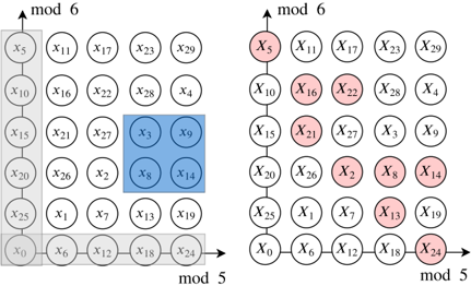
Figure 3: Example with ' = 4 secrets, and co-prime integers n 0 = 5 , n 1 = 6 , yielding N = n 0 n 1 = 30 . Zeros are placed at gray locations, and the secrets at blue locations. Careful zero padding induces parity checks on the shares in each row and column due to aliasing , i.e., » X 0 + X 5 + + X 25; X 1 + + X 26; ; X 4 + + X 29 … = » 0 ; ; 0 … and » X 0 + X 6 + + X 24; ; X 5 + + X 29 … = » 0 ; ; 0 … . Any one missing share in a row or column can be recovered using the parity-check structure. E.g., dropped out red shares can be recovered by iteratively decoding the missing shares in rows and columns.
<details>
<summary>Image 3 Details</summary>
### Visual Description
## Diagram: Modular Arithmetic Visualization
### Overview
The image presents two diagrams illustrating modular arithmetic concepts. Both diagrams are arranged as 6x5 grids, with each cell containing a variable labeled 'x' with a subscript. The left diagram highlights specific elements with gray and blue shading, while the right diagram highlights different elements with red shading. The diagrams are labeled with "mod 6" on the vertical axis and "mod 5" on the horizontal axis.
### Components/Axes
* **Axes:**
* Vertical Axis (both diagrams): Labeled "mod 6".
* Horizontal Axis (both diagrams): Labeled "mod 5".
* **Grid:** Both diagrams consist of a 6x5 grid of cells.
* **Cells:** Each cell contains a variable 'x' with a subscript ranging from 0 to 29.
* **Shading (Left Diagram):**
* Gray: Highlights the leftmost column (x5, x10, x15, x20, x25, x0) and the bottom row (x0, x6, x12, x18, x24).
* Blue: Highlights a 2x2 square in the center (x3, x9, x8, x14).
* **Shading (Right Diagram):**
* Red: Highlights specific cells: x5, x16, x22, x21, x2, x8, x14, x13, x24.
### Detailed Analysis
**Left Diagram:**
* **Grid Structure:** A 6x5 grid with 'x' variables in each cell.
* **Gray Highlight:**
* Column: x5, x10, x15, x20, x25, x0.
* Row: x0, x6, x12, x18, x24.
* **Blue Highlight:**
* Square: x3, x9, x8, x14.
**Right Diagram:**
* **Grid Structure:** Identical 6x5 grid to the left diagram.
* **Red Highlight:**
* x5 (top-left)
* x16
* x22
* x21
* x2
* x8
* x14
* x13
* x24 (bottom-right)
### Key Observations
* The left diagram highlights modular arithmetic sequences along the axes and a central square.
* The right diagram highlights a seemingly arbitrary set of cells.
* Both diagrams share the same grid structure and variable assignments.
### Interpretation
The diagrams likely illustrate modular arithmetic principles. The left diagram visually represents the remainders when dividing by 5 (horizontal axis) and 6 (vertical axis). The gray shading emphasizes the elements that are congruent to 0 mod 5 and 0 mod 6. The blue square might represent a specific calculation or property within the modular system. The right diagram could be showing the result of a specific modular operation or a set of elements that satisfy a particular modular condition. Without additional context, the exact meaning of the red highlighted cells in the right diagram is unclear, but it likely represents a specific set of solutions or outcomes within the modular arithmetic system being visualized.
</details>
The proof essentially follows from the subsampling and aliasing properties of the Fourier transform and is deferred to Appendix B.
Remark 1. When translated in coding theory parlance, the above lemma essentially states that the shares form a codeword of a product code with Reed-Solomon component codes [31]. In particular, when the shares are represented on a 2D-grid using the Chinese remainder theorem, each row (resp. column) forms a codeword of a Reed-Solomon code with block-length n 0 (resp. n 1 ) and dimension ' 1 δ 0 ' n 0 (resp. ' 1 δ 1 ' n 1 ). In other words, ¯ X c = h X c X N n i + c X ' n i 1 ' N n i + c i is a codeword of an ' n i ; ' 1 δ i ' n i ' Reed-Solomon code for every c = 0 ; 1 ; : : : ; N n i 1 . To see this, observe that when the constraints in (6) , for a fixed c , are written in a matrix form, the resulting matrix is a Vandermonde matrix, and it is straightforward to show that ¯ X c corresponds to the evaluations of a polynomial of degree ' 1 δ i ' n i 1 at ω uN n i for u = 0 ; 1 ; : : : ; n i 1 . We present a comparison with the Shamir's scheme in Appendix F.
These parity-check constraints on the shares make it possible to iteratively recover missing shares from each row and column until all the missing shares can be recovered. We present a toy example for this in Fig. 3. It is worth noting that this way of recovering the missing symbols of a codeword is known in coding theory as an iterative (bounded distance) decoder [27, 38].
In particular, codewords of a Reed-Solomon code with blocklength n i and dimension ' 1 δ i ' n i are evaluations of a polynomial of degree at most ' 1 δ i ' n i 1. Therefore, any δ i fraction of erasures can be recovered via polynomial interepolation. Therefore, if a row (resp. column) has less than δ 0 n 0 (resp. δ 1 n 1) missing shares, then they can be recovered. This process is repeated for a fixed number if iterations, or until all the missing shares are recovered.
## Algorithm 1 FastShare Secret Sharing
procedure FastShare( s ; C ) parameters: finite field F q of size q , a primitive root of unity ω in F q , privacy threshold T , dropout resilience D inputs: secret s 2 F L q , set of N clients C (client-IDs) initialize: sets Z 0, Z 1, S as per (2), (2), (4), respectively; an arbitrary bijection σ : S ! f 0 ; 1 ; : : : ; S 1 g for j = 0 to n 1 do if j 2 Z 0 [ Z 1 then x j 0 else if j 2 S then x j s σ ' j ' . s i is the i -th coordinate of s else x j $ F q end if end for X FFT ω ' x ' Output: f' i ; » s … i 'g i 2C f' i ; X i 'g N 1 i = 0 end procedure procedure FastRecon( f' i ; » s … i 'g i 2R ) parameters: finite field F q of size q , a primitive root of unity ω in F q , privacy threshold T , dropout resilience D , number of iterations J , bijection σ and set S used in FastShare input: subset of shares with client-IDs f' i ; » s … i 'g i 2R for iterations j = 1 to J do for rows r = 0 to n 1 1 in parallel do if r has fewer than δ 0 n 0 missing shares then Decode the missing share values by polynomial interpolation end if end for for columns c = 0 to n 0 1 in parallel do if c has fewer than δ 1 n 1 missing shares then Decode the missing share values by polynomial interpolation end if end for end for if any missing share then Output: ? else x I F FT ω ' X ' Output: s X ' σ 'S'' end if end procedure
Putting things together, FastRecon first uses an iterative decoder to obtain the missing shares. If the peeling decoder fails, it outputs ? , and declares failure. Otherwise, it takes the inverse (fast) Fourier transform of X (generated by ω ) to obtain x . Finally, it output the coordinates of x indexed by S (in the 2D-grid representation) as the secret. The details are given in Algorithm 1.
## 3.3 Analysis of FastShare
First, we analyze the security and correctness of FastShare in the honest-but-curious setting. We defer the proof to Appendix C.
Theorem 3.3. Given fractions δ 0 ; δ 1 ; α 2 ' 0 ; 1 ' and β 2 ' 0 ; 1 2 ' , FastShare generates N shares from S = ' 1 α '' 1 2 β '' 1 δ 0 '' 1 δ 1 ' N secrets such that it satisfies
- (1) T -privacy for T = αβ ' 1 δ 0 '' 1 δ 1 ' N ,
- (2) D -dropout resilience for D = ' 1 ' 1 δ 0 '' 1 δ 1 '' N 2 , and
- (3) linearity.
For example, choosing α = 1 2, β = 1 4, δ 0 = δ 1 = 1 10, yields S = 0 : 2 N , T = 0 : 1 N , and D = 0 : 095 N .
Computation Cost: FastShare runs in O' N log N ' time, since constructing the signal takes O' N ' time and the Fourier transform can be computed in O' N log N ' time using a Fast Fourier Transform (FFT). FastRecon also runs in O ' N log N ' time, when computations are parallelized. Specifically, recovering the missing shares in a row or column of shares (when arranged in the 2D-grid) can be done in O n 2 i = O' N ' complexity by leveraging that rows and columns are Reed-Solomon codewords, which are evaluations of a degree-' n i δ i n i 1 ' polynomial. Since all rows and columns can be decoded in parallel, and decoding is carried out for a constant number of iterations, the iterative decoder runs in O' N ' time. The second step is the inverse Fourier transform, which can be computed in O' N log N ' time using an FFT.
Next, we present the computation cost in terms of the number of (basic) arithmetic operations in F q .
Note that in practical FL scenarios, the number of clients typically scales up to ten thousand [8]. Therefore, in order to gain full parallelism, one needs to have p N 100 processors/cores. In the next section, we present a variant of FastShare that removes the requirement of parallelism for sufficiently large N . Moreover, this variant also allows us to achieve a more favorable trade-off between the number of shares, privacy threshold, and dropout tolerance.
## 3.4 Improving the Performance for Large Number of Clients
FastShare ensures that when the shares are arranged in a 2Dgrid using the Chinese remainder theorem, each row and column satisfies certain parity-check constraints (cf. Remark 1). As we show next, when N is sufficiently large, it suffices to ensure that only rows (or columns) satisfy the parity-check constraints. In this case, the FastShare algorithm remains the same as before except for the placement of secrets, zeros, and random masks changes slightly.
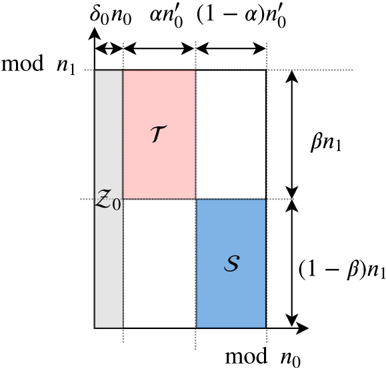
Let q be a power of a prime, and let N be a positive integer such that N divides q 1. Let c 1 be a constant. We consider N of the form N = n 0 n 1 such that n 0 = c log N . Given fractions δ 0 ; α ; β 2 ' 0 ; 1 ' , we define the sets of tuples Z 0, S , and T using the grid representation determined by the Chinese remainder theorem, as depicted in Fig. 4. We give the formal definitions below. Note that we round any rational number x to b x c , and omit the floor sign for the sake of brevity.
<!-- formula-not-decoded -->
<!-- formula-not-decoded -->
Figure 4: Indices assigned to a grid, and sets Z , S , and T . Here, we define n 0 0 = ' 1 δ 0 ' n 0 . Set S is used for secrets, Z 0 is used for zeros, and the remaining locations are used for random masks. Set T is used in our privacy proof.
<details>
<summary>Image 4 Details</summary>
### Visual Description
## Diagram: Modular Space Partitioning
### Overview
The image is a diagram illustrating the partitioning of a modular space. It shows a rectangular area divided into sections, labeled with mathematical expressions related to modular arithmetic. The diagram includes axes labeled "mod n₀" and "mod n₁", and regions marked as "T" and "S".
### Components/Axes
* **X-axis:** Labeled "mod n₀" at the bottom. The axis is divided into three segments with lengths δ₀n₀, αn'₀, and (1-α)n'₀.
* **Y-axis:** Labeled "mod n₁" on the left. The axis is divided into two segments with lengths βn₁ and (1-β)n₁.
* **Regions:**
* A gray region on the left, spanning the entire height of the rectangle and having a width of δ₀n₀.
* A pink region labeled "T" in the top-center. Its width is αn'₀ and its height is βn₁.
* A blue region labeled "S" in the bottom-center. Its width is αn'₀ and its height is (1-β)n₁.
* **Point:** A point labeled "Z₀" is located at the intersection of the gray region and the horizontal line dividing the pink and blue regions.
### Detailed Analysis or ### Content Details
* **X-axis segments:**
* Segment 1 (left): δ₀n₀
* Segment 2 (center): αn'₀
* Segment 3 (right): (1-α)n'₀
* **Y-axis segments:**
* Segment 1 (top): βn₁
* Segment 2 (bottom): (1-β)n₁
* **Region T:**
* Color: Pink
* Width: αn'₀
* Height: βn₁
* Position: Top-center
* **Region S:**
* Color: Blue
* Width: αn'₀
* Height: (1-β)n₁
* Position: Bottom-center
* **Gray Region:**
* Color: Gray
* Width: δ₀n₀
* Height: βn₁ + (1-β)n₁ = n₁
* Position: Left
* **Point Z₀:**
* Position: At the intersection of the top of the "S" region and the right edge of the gray region.
### Key Observations
* The diagram represents a modular space divided into regions based on parameters α, β, δ₀, n₀, and n₁.
* The regions T and S have the same width but different heights.
* The gray region's width is determined by δ₀n₀.
* The point Z₀ seems to be a reference point within this modular space.
### Interpretation
The diagram likely illustrates a concept in number theory or cryptography, possibly related to modular arithmetic or lattice-based cryptography. The partitioning of the space into regions T and S, along with the parameters α, β, δ₀, n₀, and n₁, likely represent different sets or conditions within the modular space. The point Z₀ could be a specific element or a reference point used in some algorithm or proof. The diagram visualizes how the modular space "mod n₀ x mod n₁" is partitioned based on the given parameters.
</details>
<!-- formula-not-decoded -->
<!-- formula-not-decoded -->
We construct the signal by placing zeros at indices in Z 0, and secrets at indices in S . Each of the remaining indices is assigned a uniform random mask from F q (independent of other masks and the secrets). We then take the Fourier transform (generated by a primitive N -th root of unity in F q ) of the signal to obtain the shares.
Using the same arguments as in the proof of Lemma 3.2, it is straightforward to show that, for every c 2 f 0 ; : : : ; n 1 1 g and v 2 f 0 ; 1 ; : : : ; δ 0 n 0 1 g , it holds that
<!-- formula-not-decoded -->
When translated in coding theory parlance, the above condition states that when the shares are represented in a 2D-grid using the Chinese remainder theorem, then each row forms a codeword of a Reed-Solomon code with block-length n 0 and dimension ' 1 δ 0 ' n 0. 4
FastRecon first recovers the missing shares by decoding each row. If every row has less than δ 0 fraction of erasures, then it recovers all the missing shares. Otherwise, it outputs ? , and declares failure. Next, it takes the inverse (fast) Fourier transform of the shares to obtain the signal. The coordinates of the signal indexed by S (in the 2D-grid representation) gives the secrets.
Security and Correctness: Given fractions δ 0 ; α ; β 2 ' 0 ; 1 ' , this variant of FastShare generates N shares from
<!-- formula-not-decoded -->
4 We note that this variant of FastShare is related to a class of erasure codes called Locally Recoverable Codes (LRCs) (see [21, 37, 44], and references therein). See Appendix F for details.
secrets such that it satisfies T -privacy for
<!-- formula-not-decoded -->
D -dropout-resilience for
<!-- formula-not-decoded -->
and linearity. (The proof is similar to Theorem 3.3, and is omitted.) Observe that this variant achieves a better trade-off between S , T , and D . For instance, choosing δ 0 = 1 10, α = 1 2, and β = 1 2, yields S = 0 : 225 N , T = 0 : 225, and D = 0 : 1.
Computation Cost: In this case, FastShare also has O' N log N ' computational cost, since constructing the signal takes O' N ' time and the Fourier transform can be computed in O' N log N ' time using an FFT. FastRecon has O' N log N ' computational cost without requiring any parallelism. In particular, recovering the missing shares in a row (when arranged in the 2D-grid) can be done in O n 2 0 = O log 2 N complexity by leveraging that the rows are Reed-Solomon codewords, which are evaluations of a degree-' n 0 δ 0 n 0 1 ' polynomial. Since there are O' N log N ' rows, the decoder to recover the missing shares has O' N log N ' complexity. The second step is the inverse FFT, which also has O' N log N ' complexity.
## 4 FASTSECAGG BASED ON FASTSHARE
In this section, we present our proposed protocol FastSecAgg, which allows the server to securely compute the summation of clients' model updates. We begin with a high-level overview of FastSecAgg (see Fig. 5). Each client generates shares for its lengthL input (by breaking it into a sequence of d L S e vectors, each of length at most S , and treating each vector as S secrets) using FastShare, and distributes the shares to N clients. Since all the communication in FL is mediated by the server, clients encrypt their shares before sending it to the server to prevent the server from reconstructing the secrets. Each client then decrypts and sums the shares it receives from other clients (via the server). The linearity property of FastShare ensures that the sum of shares is a share of the sum of secret vectors (i.e., client inputs). Each client then sends the sum-share to the server (as a plaintext). The server can then recover the sum of secrets (i.e., client inputs) with high probability as long as it receives the shares from a random set of clients of sufficient size. We note that FastSecAgg uses secret sharing as a primitive in a standard manner, similar to several secure aggregation protocols [5, 11, 22].
Round 0 consists of generating and advertising encryption keys. Specifically, each client i uses the key agreement protocol to generate a public-private key pair ' pk i ; sk i ' KA.gen ' pp ' , and sends their public key pk i to the server. The server waits for at least N D clients (denoted as C 0 C ), and forwards the received public keys to clients in C 0.
FastSecAgg is a three round interactive protocol. See Fig. 5 for a high-level overview, and Algorithm 2 for the detailed protocol. Recall that the model update for client i 2 C is assumed to be u i 2 Z L R , for some R q . In practice, this can be achieved by appropriately quantizing the updates.
Round 1 consists of generating secret shares for the updates. Each client i partitions their update u i into d L S e vectors, u 1 , u 2 , : : : ,
i
i
Figure 5: High-lever overview of FastSecAgg protocol.
<details>
<summary>Image 5 Details</summary>
### Visual Description
## Sequence Diagram: Secure Summation Protocol
### Overview
The image depicts a sequence diagram illustrating a secure summation protocol between a client and a server. The protocol is divided into three rounds: advertising keys, generating shares, and generating sum shares/reconstructing the sum. The diagram outlines the steps involved in each round, including key generation, share computation, encryption, decryption, and summation.
### Components/Axes
* **Entities:**
* Client (located at the top-left)
* Server (located at the top-right)
* **Rounds:**
* Round 0: Advertise Keys (left side)
* Round 1: Generate Shares (left side)
* Round 2: Generate sum shares/Reconstruct the sum (left side)
* **Messages:** Arrows indicate the flow of messages between the client and the server.
* **Processes:** Text descriptions detail the actions performed by each entity.
### Detailed Analysis or ### Content Details
**Round 0: Advertise Keys**
* **Client:**
* Generates an encryption key pair (k<sub>i</sub><sup>pk</sup>, k<sub>i</sub><sup>sk</sup>).
* Sends public keys k<sub>i</sub><sup>pk</sup> to the server.
* **Server:**
* Waits for enough clients C<sub>0</sub> ⊆ C.
* Sends the list of received public keys to clients in C<sub>0</sub>.
**Round 1: Generate Shares**
* **Client:**
* Computes shares of u<sub>i</sub> using FASTSHARE.
* Computes encrypted shares c<sub>i→j</sub> using the shared key.
* Sends encrypted shares c<sub>i→j</sub> to the server.
* **Server:**
* Waits for enough clients C<sub>1</sub> ⊆ C<sub>0</sub>.
* Forwards received encrypted shares to clients in C<sub>1</sub>.
**Round 2: Generate sum shares/Reconstruct the sum**
* **Client:**
* Decrypts the received shares.
* Computes the sum of shares.
* Sends the sum share sh<sub>i</sub> to the server.
* **Server:**
* Waits for enough clients C<sub>2</sub> ⊆ C<sub>1</sub>.
* Reconstructs the sum of secrets using FASTRECON.
### Key Observations
* The protocol involves three rounds of communication between the client and the server.
* Encryption and decryption are used to secure the shares.
* FASTSHARE and FASTRECON are used for share generation and reconstruction, respectively.
* The server waits for a sufficient number of clients in each round before proceeding.
* The sets of clients C<sub>0</sub>, C<sub>1</sub>, and C<sub>2</sub> are nested, with C<sub>2</sub> ⊆ C<sub>1</sub> ⊆ C<sub>0</sub> ⊆ C.
### Interpretation
The sequence diagram illustrates a secure summation protocol where a client distributes shares of a secret value to a server. The server aggregates these shares and reconstructs the sum without revealing the individual secret values. The use of encryption and specialized algorithms like FASTSHARE and FASTRECON ensures the privacy and security of the data during the process. The nested client sets (C<sub>0</sub>, C<sub>1</sub>, C<sub>2</sub>) suggest a progressive filtering or selection of clients involved in each round, potentially for efficiency or security reasons. The protocol is designed to allow the server to compute the sum of secret values held by multiple clients without learning the individual values themselves.
</details>
u d L S e i , such that the last vector has length at most S and all others have length S . Treating each u ' i as S secrets, the client computes N shares as f' j ; u ' i j 'g j 2C FastShare ' u ' i ; C' for 1 ' d L S e . For simplicity, we denote client i 's share for client j as sh i ! j = ' u 1 i j j u 2 i j j j j » u d L S e … ' .
j i The server waits for at least N D clients to respond (denoted as C 1 C 0). 5 Then, the server sends to each client i 2 C 1, all ciphertexts encrypted for it: f c j ! i g j 2C 1 nf i g .
j j i j In addition, every client receives the list of public keys from the server. Client i generates a shared key k i ; j KA.agree ' sk i ; pk j ' for each j 2 C 0 n f i g , and encrypts sh i ! j using the shared key k i ; j as c i ! j AE.enc k i ; j ; sh i ! j . The client then sends all the encrypted shares f c i ! j g 2C 0 nf g to the server.
Round 2 consists of generating sum-shares and reconstructing the approximate sum. Every surviving client receives the list of encrypted shares from the server. Each client i then decrypts the ciphertexts c j ! i using the shared key k j ; i to obtain the shares sh j ! i , i.e., sh j ! i AE.dec ' k j ; i ; c j ! i ' where k j ; i KA.agree ' sk j ; pk i ' . Then, each client i computes the sum (over F q ) of all the shares including its own share as: sh i = ˝ j 2C 1 sh j ! i . Each client i sends the sum-share sh i to the server (as a plaintext).
The server waits for at least N D clients to respond (denoted as C 2 C 1). Let sh ' i denote the ' -th coefficient of sh i for 1 ' d L S e . The server computes f z ' ; ?g FastRecon f' i ; sh ' i 'g i 2C 2 ,
5 For simplicity, we assume that a client does not drop out after initiating communication with the server, i.e., while sending or receiving messages from the server. The same assumption is also made in [3, 9, 43]. This is not a critical assumption, and the protocol and the analysis can be easily adapted if it does not hold.
## Algorithm 2 FastSecAgg Protocol
- Parties: Clients 1 ; 2 ; : : : ; N and the server
- Input: u i 2 Z L (for each client i )
- Public Parameters: Update length L , input domain Z R , key agreement parameter pp KA.param ' λ ' , finite field F q for FastShare secret sharing with primitive N -th root of unity ω
- R Output: z 2 Z L (for the server)
R
- Round 0 (Advertise Keys)
- -Generate key pairs ' pk ; sk i ' KA.gen ' pp '
Client i :
- i -Send pk to the server and move to the next round
i
- -Wait for at least N D clients to respond (denote this set as C 0 C ); otherwise, abort
## Server:
- -Send to all clients in C 0 the list f' i ; pk i 'g i 2C 0 , and move to the next round
Client i :
## Round 1 (Generate shares)
- -Receive the list f' j ; pk j 'g j 2C 0 from the server; Assert that jC 0 j N D , otherwise abort
- -Compute N shares by treating each u ' i as S secrets as f' j ; u ' i j 'g j 2C FastShare ' u ' i ; C' for 1 ' d L S e (by using independent private randomness for each ' ); Denote client i 's share for client j as sh i ! j = u 1 j j u 2 j j j j » u d L S e …
- -Partition the input u i 2 Z L R into d L S e vectors, u 1 i , u 2 i , : : : , u d L S e i , such that u d L S e i has length at most S and all others have length S
i
i
- -Send all the ciphertexts f c i ! j g 2C 0 nf g to the server by adding the addressing information i ; j as metadata
- j j j -For each client j 2 C 0 n f i g , compute encrypted share: c i ! j AE.enc ' k i ; j ; i j j j j j sh i ! j ' , where k i ; j = KA.agree ' sk i ; pk j '
- j i -Store all the messages received and values generated in this round and move to the next round
- -Wait for at least N D clients to respond (denote this set as C 1 C 0)
## Server:
- -Send to each client i 2 C 1, all ciphertexts encrypted for it: c j ! i 2C 1 nf g , and move to the next round
Client i :
- Round 2 (Recover the aggregate update)
- -Receive from the server the list of ciphertexts c j ! i j 2C 1 nf i g
- -Compute the sum of shares over F q as sh i = ˝ j 2C 1 sh j ! i
- -Decrypt the ciphertext ' i 0 j j j 0 j j sh j ! i ' Dec ' sk i ; c j ! i ' for each client j 2 C 1 n f i g , and assert that ' i = i 0 ' ^ ' j = j 0 '
- -Send the share sh i to the server
- -Wait for at least N D clients to respond (denote this set as C 2 C 1)
i
## Server:
- -Run the reconstruction algorithm to obtain z ' ; ? FastRecon ' n ' i ; sh ' i ' o i 2C 2 ' for 1 ' d L S e , where sh ' i is the ' -th coefficient of sh ; Denote z = » z 1 z 2 z d L S e …
- -Output the aggregate result z
- -If the reconstruction algorithm returns ? for any ' , then abort
for 1 ' d L S e . If the reconstruction fails (i.e., outputs ? ) for any ' , then the server aborts the current FL iteration and moves to the next one. Otherwise, it outputs z = » z 1 z 2 z d L S e … .
## 5 ANALYSIS
## 5.1 Correctness and Security
First we state the correctness of FastSecAgg, which essentially follows from the linearity and D -dropout tolerance of FastShare. The proof is given in D.
Theorem 5.1 (Correctness). Let f u i g i 2C denote the client inputs for FastSecAgg. If a random set of at most D clients drop out during the execution of FastSecAgg, i.e., jC 2 j N D , then the server does not abort and obtains z = ˝ i 2C 1 u i with probability at least 1 1 poly N , where the probability is over the randomness in dropouts.
Next, we show that FastSecAgg is secure against the server colluding with up to T clients in the honest-but-curious setting, irrespective of how and when clients drop out. Specifically, we prove that the joint view of the server and any set of clients of bounded size does not reveal any information about the updates of the honest clients, besides what can be inferred from the output of the summation.
We will consider executions of FastSecAgg where FastShare has privacy threshold T , and the underlying cryptographic primitives are instantiated with security parameter λ . We denote the server (i.e., the aggregator) as A , and the set of of N clients as C .
j
i
i
Clients may drop out (or, abort) at any point during the execution, and we denote with C i the subset of the clients that correctly sent their message to the server in round i . Therefore, we have C C 0 C 1 C 2. For example, the set C 0 n C 1 are the clients that abort before sending the message to the server in Round 1, but after sending the message in Round 0. Let u i 2 Z L R denote the model update of client i (i.e., u i the i -th client's input to the secure aggregation protocol), and for any subset C 0 C , let u C 0 = f u i g i 2C 0 .
In such a protocol execution, the view of a participant consists of their internal state (including their update, encryption keys, and randomness) and all messages they received from other parties. Note that the messages sent by the participant are not included in the view, as they can be determined using the other elements of their view. If a client drops out (or, aborts), it stops receiving messages and the view is not extended past the last message received.
Given any subset M C , let REAL C ; T ; λ M ' u C ; C 0 ; C 1 ; C 2 ' be a random variable representing the combined views of all parties in M[f A g in an execution of FastSecAgg, where the randomness is over the internal randomness of all parties, and the randomness in the setup phase. We show that for any such set M of honest-butcurious clients of size up to T , the joint view of M[f A g can be simulated given the inputs of the clients in M , and only the sum of the values of the remaining clients.
Theorem 5.2 (Security). There exists a probabilistic polynomial time (PPT) simulator SIM such that for all C , u C , C 0 , C 1 , C 2 , and M such that M C , jMj T , C C 0 C 1 C 2 , the output of SIM is computationally indistiguishable from the joint view REAL C ; T ; λ M of the server and the corrupted clients M , i.e.,
<!-- formula-not-decoded -->
where
<!-- formula-not-decoded -->
The security and correctness of FastSecAgg critically relies on the guarantees provided by FastShare proved in Theorem 3.3. We present the proofs of the above theorem in Appendices E.
## 5.2 Computation and Communication Costs
We assume that the addition and multiplication operations in F q are O' 1 ' each.
Computation Cost at a Client: O' max f L ; N g log N ' . Each client's computation cost can be broken as computing shares using FastShare which is O'd L S e N log N ' = O' max f L ; N g log N ' ; encrypting and decrypting shares, which is O'd L S e N ' ; and adding the received shares, which is O'd L S e N ' = O' max f L ; N g' .
CommunicationCostataClient: O' max f L ; N g' . Each client sends and receives N 1 shares (each having d L S e elements in F q ), resulting in O'd L S e N ' = O' max f L ; N g' communication. In addition, each client sends the sum-share consisting of d L S e elements in F q .
Computation Cost at the Server: O' max f L ; N g log N ' . The server first recovers missing sum-shares using FastRecon, each has d L S e elements in F q . This results in O'd L S e N log N ' complexity.
The second step is the inverse FFT on N shares, each has of d L S e elements in F q , resulting in O'd L S e N log N ' complexity.
Communication Cost at the Server: O' N max f L ; N g' . The server communicates N times of what each client communicates.
## 5.3 Comparison with Prior Works
Bonawitz et al. [9] presented the first secure aggregation protocol SecAgg for FL, wherein clients use a key exchange protocol to agree on pairwise additive masks to achieve privacy. SecAgg, in the honest-but-curious setting, can achieve T = αN for any α 2 ' 0 ; 1 ' and D = N T 1, and provides worst-case dropout resilience, i.e., it can tolerate any D users dropping out. However, SecAgg incurs significant computation cost of O LN 2 at the server. This limits its scalability to several hundred clients as observed in [8].
The scheme by So et al. [43], which we call TurboAgg, uses additive secret sharing for security combined with erasure codes for dropout tolerance. TurboAgg allows T = D = αN for any α 2 ' 0 ; 1 2 ' . However, it has two main drawbacks. First, it divides N clients into N log N groups, and each client in a group needs to communicate to every client in the next group. This results in per client communication cost of O' L log N ' . Moreover, processing in groups requires at least log N rounds. Second, it can tolerate only non-adaptive adversaries, i.e., client corruptions happen before the clients are partitioned into groups. On the other hand, FastSecAgg results in O' L ' communication per client, runs in 3 rounds, and is robust against an adaptive adversary which can corrupt clients during the protocol execution.
Truex et al. [45] uses threshold homomorphic encryption and Xu et al. [47] uses functional encryptionto perform secure aggregation. However, these schemes assume a trusted third party for key distribution, which typically does not hold in the FL setup.
Recently, Bell et al. [3] proposed an improved version of SecAgg, which we call SecAgg+. Their key idea is to replace the complete communication graph of SecAgg by a sparse random graph to reduce the computation and communication costs. FastSecAgg achieves smaller computation cost than SecAgg+ at the server and the same (orderwise) communication cost per client as SecAgg+ when L = Ω ' N ' . Moreover, FastSecAgg is robust against adaptive adversaries, whereas SecAgg+ can mitigate only non-adaptive adversaries where client corruptions happen before the protocol execution starts. On the other hand, SecAgg+ achieves smaller communication cost in absolute numbers than FastSecAgg.
There are several recent works [24, 35, 42] which consider secure aggregation when a fraction of clients are Byzantine. Our focus, on the other hand, is on honest-but-curious setting, and we leave the case of Byzantine clients as a future work.
The performance comparison between FastSecAgg and SecAgg [9], TurboAgg [43], and SecAgg+ [3] is summarized in Table 1.
## ACKNOWLEDGEMENTS
Swanand Kadhe was introduced to the secure aggregation problem in the Decentralized Security course by Raluca Ada Popa in Fall 2019. He would like to thank Raluca for an excellent course. Swanand would like to thank Mukul Kulkarni for immensely helpful discussions and for providing feedback on drafts of this paper.
This work is supported in part by the National Science Foundation grant CNS-1748692.
## REFERENCES
- [1] Gergely ´ Acs and Claude Castelluccia. 2011. I Have a DREAM! Differentially Private Smart Metering. In Proceedings of the 13th International Conference on Information Hiding (IH'11) . Springer-Verlag, Berlin, Heidelberg, 118-132.
- [3] James Bell, K. A. Bonawitz, Adri` a Gasc´ on, Tancr` ede Lepoint, and Mariana Raykova. 2020. Secure Single-Server Aggregation with (Poly)Logarithmic Overhead. Cryptology ePrint Archive, Report 2020/704. (2020). https://eprint.iacr. org/2020/704.
- [2] Amos Beimel. 2011. Secret-Sharing Schemes: A Survey. In Coding and Cryptology , Yeow Meng Chee, Zhenbo Guo, San Ling, Fengjing Shao, Yuansheng Tang, Huaxiong Wang, and Chaoping Xing (Eds.). Springer Berlin Heidelberg, Berlin, Heidelberg, 11-46.
- [4] Mihir Bellare and Chanathip Namprempre. 2000. Authenticated Encryption: Relations among Notions and Analysis of the Generic Composition Paradigm. In Advances in Cryptology - ASIACRYPT 2000 , Tatsuaki Okamoto (Ed.). 531-545.
- [6] R. E. Blahut. 1979. Transform Techniques for Error Control Codes. IBM Journal of Research and Development 23, 3 (1979), 299-315.
- [5] Michael Ben-Or, Shafi Goldwasser, and Avi Wigderson. 1988. Completeness Theorems for Non-Cryptographic Fault-Tolerant Distributed Computation. In Proceedings of the Twentieth Annual ACM Symposium on Theory of Computing (STOC '88) . Association for Computing Machinery, New York, NY, USA, 1-fi/question\_exclam10. https://doi.org/10.1145/62212.62213
- [7] Carlo Blundo, Alfredo De Santis, Giovanni Di Crescenzo, Antonio Giorgio Gaggia, and Ugo Vaccaro. 1994. Multi-Secret Sharing Schemes. In Advances in Cryptology - CRYPTO '94 , Yvo G. Desmedt (Ed.). Springer Berlin Heidelberg, Berlin, Heidelberg, 150-163.
- [9] Keith Bonawitz, Vladimir Ivanov, Ben Kreuter, Antonio Marcedone, H. Brendan McMahan, Sarvar Patel, Daniel Ramage, Aaron Segal, and Karn Seth. 2017. Practical Secure Aggregation for Privacy-Preserving Machine Learning. In Proceedings of the 2017 ACM SIGSAC Conference on Computer and Communications Security (CCS '17) . 1175-1191.
- [8] Keith Bonawitz, Hubert Eichner, Wolfgang Grieskamp, Dzmitry Huba, Alex Ingerman, Vladimir Ivanov, Chlo M Kiddon, Jakub Koneff\_hn, Stefano Mazzocchi, Brendan McMahan, Timon Van Overveldt, David Petrou, Daniel Ramage, and Jason Roselander. 2019. Towards Federated Learning at Scale: System Design. In Proceedings of the 2nd SysML Conference .
- [10] A. Borodin and R. Moenck. 1974. Fast modular transforms. J. Comput. System Sci. 8, 3 (1974), 366 - 386. https://doi.org/10.1016/S0022-0000(74)80029-2
- [12] B. Cakici, K. Hebing, M Grunewald, P. Saretok, and A. Hulth. 2010. CASE: a framework for computer supported outbreak detection. In BMC Medical Information and Decision Making .
- [11] Martin Burkhart, Mario Strasser, Dilip Many, and Xenofontas Dimitropoulos. 2010. SEPIA: Privacy-Preserving Aggregation of Multi-Domain Network Events and Statistics. In Proceedings of the 19th USENIX Conference on Security (USENIX Security'10) . USENIX Association, USA, 15.
- [13] Nicholas Carlini, Chang Liu, ´ Ulfar Erlingsson, Jernej Kos, and Dawn Song. 2019. The Secret Sharer: Evaluating and Testing Unintended Memorization in Neural Networks. In 28th USENIX Security Symposium (USENIX Security 19) . 267-284.
- [15] David Evans, Vladimir Kolesnikov, and Mike Rosulek. 2018. A Pragmatic Introduction to Secure Multi-Party Computation. Foundations and Trends in Privacy and Security 2 (2018), 70-246.
- [14] John R. Douceur. 2002. The Sybil Attack. In Peer-to-Peer Systems . Springer Berlin Heidelberg, Berlin, Heidelberg, 251-260.
- [16] Matthew Franklin and Moti Yung. 1992. Communication Complexity of Secure Computation (Extended Abstract). In Proceedings of the Twenty-Fourth Annual ACM Symposium on Theory of Computing . 699-710.
- [18] Clement Fung, Chris J. M. Yoon, and Ivan Beschastnikh. 2018. Mitigating Sybils in Federated Learning Poisoning. CoRR abs/1808.04866 (2018). arXiv:1808.04866 http://arxiv.org/abs/1808.04866
- [17] Matt Fredrikson, Somesh Jha, and Thomas Ristenpart. 2015. Model Inversion Attacks That Exploit Confidence Information and Basic Countermeasures. In Proceedings of the 22nd ACM SIGSAC Conference on Computer and Communications Security . 1322-1333.
- [19] Karan Ganju, Qi Wang, Wei Yang, Carl A. Gunter, and Nikita Borisov. 2018. Property Inference Attacks on Fully Connected Neural Networks Using Permutation Invariant Representations. In Proceedings of the 2018 ACM SIGSAC Conference on Computer and Communications Security . 619-633.
- [21] P. Gopalan, Cheng Huang, H. Simitci, and S. Yekhanin. 2012. On the Locality of Codeword Symbols. Information Theory, IEEE Transactions on 58, 11 (Nov 2012), 6925-6934.
- [20] Joachim Von Zur Gathen and Jurgen Gerhard. 2003. Modern Computer Algebra (2 ed.). Cambridge University Press, USA.
- [22] S. Goryczka and L. Xiong. 2017. A Comprehensive Comparison of Multiparty Secure Additions with Differential Privacy. IEEE Transactions on Dependable and Secure Computing 14, 5 (2017), 463-477.
- [24] Lie He, Sai Praneeth Karimireddy, and Martin Jaggi. 2020. Secure ByzantineRobust Machine Learning. (2020). arXiv:cs.LG/2006.04747
- [23] K. He, X. Zhang, S. Ren, and J. Sun. 2016. Deep Residual Learning for Image Recognition. In 2016 IEEE Conference on Computer Vision and Pattern Recognition (CVPR) . 770-778.
- [25] Ellis Horowitz. 1972. A fast method for interpolation using preconditioning. Inform. Process. Lett. 1, 4 (1972), 157 - 163. https://doi.org/10.1016/0020-0190(72) 90050-6
- [27] J. Justesen. 2011. Performance of Product Codes and Related Structures with Iterated Decoding. IEEE Transactions on Communications 59, 2 (2011), 407-415.
- [26] Marek Jawurek, Martin Johns, and Florian Kerschbaum. 2011. Plug-In Privacy for Smart Metering Billing. In Privacy Enhancing Technologies , Simone Fischer-H¨ ubner and Nicholas Hopper (Eds.). Springer Berlin Heidelberg, Berlin, Heidelberg, 192-210.
- [28] Peter Kairouz, H. Brendan McMahan, Brendan Avent, Aur´ elien Bellet, Mehdi Bennis, Arjun Nitin Bhagoji, Keith Bonawitz, Zachary Charles, Graham Cormode, Rachel Cummings, Rafael G. L. D'Oliveira, Salim El Rouayheb, David Evans, Josh Gardner, Zachary A. Garrett, Adri` a Gasc´ on, Badih Ghazi, Phillip B. Gibbons, Marco Gruteser, Za¨ ıd Harchaoui, Chaoyang He, Lie He, Zhouyuan Huo, Ben Hutchinson, Justin Hsu, Martin Jaggi, Tara Javidi, Gauri Joshi, Mikhail Khodak, Jakub Konecn´ y, Aleksandra Korolova, Farinaz Koushanfar, Oluwasanmi Koyejo, Tancr` ede Lepoint, Yang Liu, Prateek Mittal, Mehryar Mohri, Richard Nock, Ayfer ¨ Ozg¨ ur, Rasmus Pagh, Mariana Raykova, Hang Qi, Daniel Ramage, Ramesh Raskar, Dawn Xiaodong Song, Weikang Song, Sebastian U. Stich, Ziteng Sun, Ananda Theertha Suresh, Florian Tram` er, Praneeth Vepakomma, Jianyu Wang, Li Xiong, Zheng Xu, Qiang Yang, Felix X. Yu, Han Yu, and Sen Zhao. 2019. Advances and Open Problems in Federated Learning. ArXiv abs/1912.04977 (2019).
- [30] M. G. Luby, M. Mitzenmacher, M. A. Shokrollahi, and D. A. Spielman. 2001. Efficient erasure correcting codes. IEEE Transactions on Information Theory 47, 2 (2001), 569-584.
- [29] M. G. Luby, M. Amin Shokrolloahi, M. Mizenmacher, and D. A. Spielman. 1998. Improved low-density parity-check codes using irregular graphs and belief propagation. In Proceedings. 1998 IEEE International Symposium on Information Theory . 117-121.
- [31] F.J. MacWilliams and N.J.A. Sloane. 1978. The Theory of Error-Correcting Codes (2nd ed.). North-holland Publishing Company.
- [33] M. Nasr, R. Shokri, and A. Houmansadr. 2019. Comprehensive Privacy Analysis of Deep Learning: Passive and Active White-box Inference Attacks against Centralized and Federated Learning. In 2019 IEEE Symposium on Security and Privacy (SP) . 739-753.
- [32] Brendan McMahan, Eider Moore, Daniel Ramage, Seth Hampson, and Blaise Aguera y Arcas. 2017. Communication-Efficient Learning of Deep Networks from Decentralized Data. In Proceedings of the 20th International Conference on Artificial Intelligence and Statistics . 1273-1282.
- [34] S. Pawar and K. Ramchandran. 2018. FFAST: An Algorithm for Computing an Exactly k -Sparse DFT in O ' k log k ' Time. IEEE Transactions on Information Theory 64, 1 (2018), 429-450.
- [36] John M. Pollard. 1971. The fast Fourier transform in a finite field. Math. Comp. 25 (1971), 365-374.
- [35] Krishna Pillutla, Sham M. Kakade, and Zaid Harchaoui. 2019. Robust Aggregation for Federated Learning. (2019). arXiv:stat.ML/1912.13445
- [37] N. Prakash, G.M. Kamath, V. Lalitha, and P.V. Kumar. 2012. Optimal linear codes with a local-error-correction property. In Information Theory Proceedings (ISIT), 2012 IEEE International Symposium on . 2776-2780.
- [39] Adi Shamir. 1979. How to Share a Secret. Commun. ACM 22, 11 (Nov. 1979), 612-613.
- [38] T. J. Richardson and R. L. Urbanke. 2001. The capacity of low-density parity-check codes under message-passing decoding. IEEE Transactions on Information Theory 47, 2 (2001), 599-618.
- [40] R. Shokri, M. Stronati, C. Song, and V. Shmatikov. 2017. Membership Inference Attacks Against Machine Learning Models. In 2017 IEEE Symposium on Security and Privacy (SP) . 3-18.
- [42] Jinhyun So, Basak Guler, and A. Salman Avestimehr. 2020. Byzantine-Resilient Secure Federated Learning. (2020). arXiv:cs.CR/2007.11115
- [41] D. Silva and F. R. Kschischang. 2011. Universal Secure Network Coding via Rank-Metric Codes. IEEE Transactions on Information Theory 57, 2 (Feb. 2011), 1124-1135.
- [43] Jinhyun So, Basak Guler, and Amir Salman Avestimehr. 2020. Turbo-Aggregate: Breaking the Quadratic Aggregation Barrier in Secure Federated Learning. CoRR abs/2002.04156 (2020). https://arxiv.org/abs/2002.04156
- [45] Stacey Truex, Nathalie Baracaldo, Ali Anwar, Thomas Steinke, Heiko Ludwig, Rui Zhang, and Yi Zhou. 2019. A Hybrid Approach to Privacy-Preserving Federated Learning. In Proceedings of the 12th ACM Workshop on Artificial Intelligence and
- [44] I. Tamo and A. Barg. 2014. A Family of Optimal Locally Recoverable Codes. Information Theory, IEEE Transactions on 60, 8 (Aug 2014), 4661-4676.
Security . 1-11.
- [47] Runhua Xu, Nathalie Baracaldo, Yi Zhou, Ali Anwar, and Heiko Ludwig. 2019. HybridAlpha: An Efficient Approach for Privacy-Preserving Federated Learning. In Proceedings of the 12th ACM Workshop on Artificial Intelligence and Security (AISec'19) . Association for Computing Machinery, New York, NY, USA, 13-fi/question\_exclam23. https://doi.org/10.1145/3338501.3357371
- [46] Michael M. Wagner. 2006. CHAPTER 1 - Introduction. In Handbook of Biosurveillance , Michael M. Wagner, Andrew W. Moore, and Ron M. Aryel (Eds.). Academic Press, Burlington, 3 - 12. https://doi.org/10.1016/B978-012369378-5/50003-X
## A FINITE FIELD FOURIER TRANSFORM
Here, we review the basics of the finite field Fourier transform, for details, see, e.g., [36]. Let q be a power of a prime, and consider a finite field F q of order q . Let N be a positive integer such that N divides ' q 1 ' and ω be a primitive N -th root of unity in F q . The discrete Fourier transform (DFT) of length N generated by ω is a mapping from F N q to F N q defined as follows. Let x = » x 0 x 1 : : : x N 1 … be a vector over F q . Then, the DFT of x generated by ω , denoted as DFT ω ' x ' , is the vector over F q , X = » X 0 X 1 : : : X N 1 … , given by
<!-- formula-not-decoded -->
The inverse DFT (IDFT), denoted as I DFT ω ' X ' , is given by
<!-- formula-not-decoded -->
where 1 N denotes the reciprocal of the sum of N ones in the field F q . We refer to x as the 'time-domain signal' and index i as time, and X as the 'frequency-domain signal' or the 'spectrum' and j as frequency.
If a signal is subsampled in the time-domain, its frequency components mix together, i.e., alias , in a pattern that depends on the sampling procedure. In particular, let n be a positive integer that divides N . Let x '# n ' denote the subsampled version of x with period n , i.e., x '# n ' = f x ni : 0 i N n 1 g . Then, ' N n ' -length DFT of x '# n ' , X '# n ' , (generated by ω n ) is related to the N -length DFT of x , X , (generated by ω ) as
<!-- formula-not-decoded -->
where 1 n is the reciprocal of the sum of n ones in F q .
A circular shift in the time-domain results in a phase shift in the frequency-domain. Given a signal x , consider its circularly shifted version x ' 1 ' defined as x ' 1 ' i = x ' i + 1 ' mod N . Then, the DFTs of x ' 1 ' and x (both generated by ω ) are related as X ' 1 ' j = ω j X j . In general, a circular shift of t results in
<!-- formula-not-decoded -->
## B PROOF OF LEMMA
Proof of Lemma 3.2. For i 2 f 0 ; 1 g , for v 2 f 0 ; 1 ; : : : ; δ i n i 1 g , let us denote x ' v ''# n i ' as x circularly shifted (in advance) by v and then subsampled by n i . That is, x ' v ''# n i ' j = x ' jn i + v ' mod n i for j = 0 ; 1 ; : : : ; N n i 1. Let X ' v ''# n i ' denote the DFT of x ' v ''# n i '
generated by ω n i . Now, from the aliasing property (18), it holds that
<!-- formula-not-decoded -->
for v = 0 ; 1 ; : : : ; δ i n i 1 and c = 0 ; 1 ; : : : ; N n i 1 : However, from the circular shift property (19), we have X ' v ' j = ω vj X j for j = 0 ; 1 ; : : : ; N 1. Thus, we have
<!-- formula-not-decoded -->
for v = 0 ; 1 ; : : : ; δ i n i 1, and c = 0 ; 1 ; : : : ; N n i 1. Note that, by construction, x ' v ''# n i ' is a length-' N n i ' zero vector for v = 0 ; 1 ; : : : ; δ i n i 1 for each i 2 f 0 ; 1 g . Therefore, X ' v ''# n i ' is also a length-' N n i ' zero vector for v = 0 ; 1 ; : : : ; δ i n i 1 for each i 2 f 0 ; 1 g . Hence, from (21), we get
<!-- formula-not-decoded -->
for v = 0 ; 1 ; : : : ; δ i n i 1, and c = 0 ; 1 ; : : : ; N n i 1. Simplifying the above, we get
<!-- formula-not-decoded -->
for u = 0 ; 1 ; : : : ; n i 1, v = 0 ; 1 ; : : : ; δ i n i 1, and c = 0 ; 1 ; ; : : : ; N n i 1.
## C ANALYSIS OF FASTSHARE
We first focus on the correctness, i.e., dropout tolerance. To prove that FastShare has a dropout tolerance of D , we need to show that FastRecon can recover the secrets from a random subset of N D shares. This is equivalent to showing that the iterative peeling decoder of FastRecon can recover all the shares from a random subset of N D shares. Note that the shares generated by FastShare form a codeword of a product code. From the density evolution analysis of the iterative peeling decoder of product codes in [27, 34], it follows that, when D ' 1 ' 1 δ 0 '' 1 δ 1 '' N 2 , the decoder recovers all the shares from a random subset of N D shares with probability at least 1 poly N . Therefore, FastShare has the dropout tolerance of D = ' 1 ' 1 δ 0 '' 1 δ 1 '' N 2 .
First, we show that the information-theoretic security condition is equivalent to a specific linear algebraic condition. To this end, we first observe that the vector of N shares can be written as,
To prove the privacy threshold of T , we consider the informationtheoretic equivalent of the security definition [7]. In particular, we need to show the following: for any P C such that jPj T , it holds that H ' s j f» s … i g i 2P ' = H ' s ' , where H denotes the Shannon entropy. For simplicity, let us denote » s … i = X i for all i . In the remainder of the proof, we denote random variables by boldface letters.
<!-- formula-not-decoded -->
where s 2 F ' q is the vector of secrets, m 2 F K ' q is a vector with each element chosen independently and uniformly from F q , and G is a particular submatrix of the DFT matrix whose formal definition we defer later on. We then show that information theoretic security is equivalent to a particular linear algebraic condition on submatrices of G . To prove this condition we leverage the fact that G is derived from a DFT matrix and consider an alternate representation based on the Chinese Remainder theorem (CRT). We furnish more details while formally discussing the lemmas.
Recall that n 0 and n 1 are co-prime. By the CRT, we may conclude that any number j 2 f 0 ; ; N 1 g can be uniquely represented in a 2D-grid as a tuple ' a ; b ' where a = j mod n 0 and b = j mod n 1. First, define the set of indices
<!-- formula-not-decoded -->
Similarly, define
<!-- formula-not-decoded -->
<!-- formula-not-decoded -->
For a pictorial representation of these indices, refer to Fig. 2. These sets correspond to points in the grid, and by the CRT map back to integers in the range f 0 ; ; N 1 g .
Remark 2. In Theorem 3.3, the number of secrets ' , is chosen to be equal to ' 1 α '' 1 2 β '' 1 δ 0 '' 1 δ 1 ' n 0 n 1 . By design this coincides with the size of S .
With these definition, we next describe the construction of the matrix G is obtained by starting with the N N DFT matrix, removing the columns corresponding to Z 0 [ Z 1, and permuting the remaining columns so that the columns corresponding to S are ordered as the first ' columns in S (in arbitrary sequence).
The proof is similar to Lemma 6 in [41], and thus omitted.
Having defined the matrix G , in the following lemma we show that information theoretic security can be guaranteed by a particular rank condition satisfied by submatrices of G . In particular, In addition, define K = N jZ 0 [ Z 1 j .
Lemma C.1. Let s 2 F ' q , m 2 F k ' q , and X = G » s m … T be random variables representing the secrets, random masks, and shares, respectively. Let X P be an arbitrary set of shares corresponding to the indices in P f 1 ; 2 ; : : : ; N g . Let G P denote the sub-matrix of G corresponding to the rows indexed by P . Let G P = » G 1 G 2 … , where G 1 consists of the first ' columns of G P and G 2 consists of the last K ' columns of G P . If m is uniform over F K ' q , then it holds that
<!-- formula-not-decoded -->
Now, to prove the information-theoretic security, it suffices to prove that for any P of size at most T = αβ ' 1 δ 0 '' 1 δ 1 ' N , rank ' G 2 ' = rank ' G P ' . We prove this by showing that, for any D with jPj T , the columns of G 1 lie in the span of the columns of G 2. Note that columns of G 1 are the columns of the DFT matrix indexed by S .
Proof of rank ' G P ' = rank ' G 2 ' : Assume that f ω @ : @ 2 Pg are the set of primitive elements generating the rows of G P . For the rest of the proof we are guided by the grid representation of fig. 2 - the Chinese remainder theorem (CRT) furnishes a representation of the columns of G P , indexed by f 0 ; ; n 1 g as points on a 2D-grid, f' p 0 ; p 1 ' : p 0 2 f 0 ; ; n 0 1 g ; p 1 2 f 0 ; ; n 1 1 gg .
Notation: In the grid representation, consider the set of points T in fig. 2. Formally,
<!-- formula-not-decoded -->
Define G 2 'T' as the matrix G 2 only populated by the columns whose indices belong to T . Henceforth, we use the terminology 'points' to refer to a column of G P in its representation as a tuple in the 2D-grid. Moreover we use the terminology 'span' and 'rank' of the points to indicate the span and rank of the corresponding columns. Consider a column index p 2 f 0 ; ; n 1 g and ∆ 2 f 0 ; ; n 1 g where p 7!' p 0 ; p 1 ' and ∆ 7!' ∆ 0 ; ∆ 1 ' under the CRT bijection. Then, the notation ' p 0 ; p 1 ' + ' ∆ 0 ; ∆ 1 ' returns the point '' p 0 + ∆ 0 ' mod n 0 ; ' p 1 + ∆ 1 ' mod n 1 ' .
Observe that P + ∆ corresponds to multiplying the columns indexed by P by a full-rank matrix. Then, using the structure of G P inherited from the DFT (Vandermonde) matrix structure, we get the following result immediately.
Since G P is derived from a DFT matrix, this in fact corresponds to multiplying the column corresponding to p by the matrix diag '' ω ∆ @ : @ 2 P'' . The notations (i) p + ∆ , (ii) p + ' ∆ 0 ; ∆ 1 ' are defined analogously. We also use the terminology 'shift p horizontally by ∆ 0' and 'shift p vertically by ∆ 1' to respectively denote p + ' ∆ 0 ; 0 ' and p + ' 0 ; ∆ 1 ' . Given a set of points P , we overload notation and use P + ∆ as the set of points f p + ∆ : p 2 Pg .
Lemma C.2. If p 2 span 'P' for some set of points P , then for any ∆ 2 f 0 ; ; n 1 g , p + ∆ 2 span 'P + ∆ ' .
Proof. If p 2 span 'P' this implies that there exists weights f α q : q 2 Pg such that for each @ 2 P , ω p @ = ˝ q 2P α q ω q @ . Fixing any @ 2 P , and multiplying both sides by ω ∆ ,
@
<!-- formula-not-decoded -->
Since this is true for each @ 2 P the proof follows immediately.
By construction of the set, observe that the number of points in T equals αβ ' 1 δ 0 '' 1 δ 1 ' n 0 n 1. Moreover, recalling the choice of the privacy threshold T in Theorem 3.3, observe that jT j = T . By this fact, we have that rank ' G P ' T . This implies two possibilities:
Case I. If rank ' G 2 'T'' = rank ' G P ' , then the remaining columns in G 1 must lie in the span of G 2 'T' , and the proof concludes.
Case II. If not, then the columns of G 2 'T' must have at least one column dependent on the others.
We can identify one such column by the following procedure: starting at the top left corner of T in the grid, sequentially collect the points in T in a top-to-bottom, left-to-right sequence. Stop at the first point y = ' y 0 ; y 1 ' which lies in the span of the previously collected points (by assumption, such a point must exist as we are in Case II). Figure 6 illustrates this procedure where we collect the black points sequentially until the yellow point is reached which is the first point that lies in the span of the previously collected points. Let B be defined as the set of black points which are enumerated
Figure 6: Enumerating the columns in the bottom-right sequence until the first column (yellow) is reached which lies in the span of the previous columns
<details>
<summary>Image 6 Details</summary>
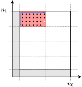
### Visual Description
## Diagram: Grid with Highlighted Region
### Overview
The image is a diagram of a grid, with a specific rectangular region highlighted in red. Black dots are distributed within this red region, and a single yellow dot is also present. Blue arrows indicate a path along the perimeter of the red region. The axes are labeled n0 and n1.
### Components/Axes
* **X-axis:** Labeled "n0" at the bottom-right corner.
* **Y-axis:** Labeled "n1" at the top-left corner.
* **Grid:** The grid consists of dashed lines, dividing the space into equal squares.
* **Highlighted Region:** A rectangular region in the top-left quadrant is highlighted in red.
* **Dots:** Multiple black dots are distributed within the red region. A single yellow dot is also present within the red region.
* **Arrows:** Blue arrows trace a path along the top and left edges of the red region.
* **Grey Shading:** The bottom-right corner and the bottom-left corner are shaded in grey.
### Detailed Analysis
* The red highlighted region spans approximately 2 grid units along the n0 axis and 2 grid units along the n1 axis.
* The black dots are arranged in a grid-like pattern within the red region. There are approximately 6 rows and 5 columns of black dots.
* The yellow dot is located near the bottom-right corner of the red region.
* The blue arrows indicate a path starting from the bottom-left corner of the red region, moving right along the top edge, and then down along the left edge.
### Key Observations
* The diagram emphasizes a specific rectangular region within a larger grid.
* The distribution of black dots within the red region suggests a structured arrangement.
* The yellow dot may represent a specific point of interest within the highlighted region.
* The blue arrows indicate a specific traversal path along the perimeter of the highlighted region.
### Interpretation
The diagram likely represents a concept related to grid-based data or algorithms. The highlighted region could represent a subset of data being processed, and the dots could represent individual data points. The yellow dot might represent a specific data point being analyzed or a target location. The blue arrows could represent the steps of an algorithm operating on the data within the highlighted region. The grey shading in the corners might represent areas outside the scope of the current operation. The diagram could be used to illustrate concepts in image processing, data analysis, or algorithm design.
</details>
until y is found. By definition, this implies that there exist (not necessarily unique) weights f α b g b 2B such that,
<!-- formula-not-decoded -->
This implies that y ' 0 ; 1 ' 2 span 'B ' 0 ; 1 '' . Define Y as the set of points,
<!-- formula-not-decoded -->
Note that the set of points Y implicitly depends on the location of point y . Next, we define L and C to be the set of points,
<!-- formula-not-decoded -->
<!-- formula-not-decoded -->
In addition, we define Q to be the set of points,
<!-- formula-not-decoded -->
Pictorially these points are represented in Figs 7 and 8.
Claim 1. Y span 'C' .
Proof. We prove this result by induction sequentially iterating over all the points from top to bottom in Y . Clearly B C , therefore the induction holds for the first point in Y , which is y = ' y 0 ; y 1 ' .
Suppose for some k 1 that for each t k 1 the point y ' 0 ; t ' lies in span 'C' . Then we show that y ' 0 ; k ' 2 span 'C' as long as k y 1 n 1 ' 1 δ 1 '' 1 β ' + 1. Indeed, observe first that,
<!-- formula-not-decoded -->
The key observation is that B ' 0 ; k ' is always C[f y ' 0 ; t ' : 0 t k 1 g (unless k > y 1 n 1 ' 1 δ 1 '' 1 β ' + 1, in which case B' 0 ; k ' shifts far enough down that it includes points in Z 1 - this has null intersection with C and Y so the assertion is clearly false). For a pictorial presentation of this fact, refer to Fig. 9. By the induction hypothesis, for each t k 1, y ' 0 ; t ' 2 span 'C' . Therefore, span 'B ' 0 ; k '' span 'C' . Plugging into eq. (36) completes the proof of the claim.
Claim 2. L span 'Q' .
Proof. Recall that L = [ n 0 y 0 1 k = 0 'Y + ' k ; 0 '' . Wefollow a similar proof by induction strategy as Claim 1 to result in the assertion. In particular, for k = 0 the statement follows directly from the fact that C Q and using Claim 1 to claim that Y span 'C' . Assuming the induction hypothesis that for all 0 t k 1, Y + ' t ; 0 ' span 'Q' we show that Y + ' k ; 0 ' span 'Q' as long as k n 0 y 0 1. In particular, observe that from Claim 1,
<!-- formula-not-decoded -->
Next observe that unless k > n 0 y 0 1,
<!-- formula-not-decoded -->
if k > n 0 y 0 1, then C + ' k ; 0 ' shifts far enough that it wraps around and include points in Z 0 - this has null intersection with Q and Y + ' t ; 0 ' for any t n 0 y 0 1 and the assertion becomes false. A pictorial representation of this fact is provided in Fig. 10. By the induction hypothesis for each 0 t k 1, Y + ' t ; 0 ' span 'Q' . Combining this fact with eqs. (37) and (38) implies that Y + ' 0 ; k ' span 'Q' and completes the induction step for k .
Recall from eq. (33) that L is defined as the set of points, [ n 0 y 0 1 k = 0 'Y + ' k ; 0 '' . More explicitly, noting that the set of points Y is defined as f' y 0 ; θ ' : y 1 n 1 ' 1 δ 1 '' 1 β ' + 1 θ y 1 g ,
<!-- formula-not-decoded -->
Claim 3. The set of points S L irrespective of the location of the point y = ' y 0 ; y 1 ' (note that the set of points L is a function of y 0 and y 1 ).
Proof. Before furnishing the details of the proof, note that a pictorial representation of this statement is provided in Fig. 10. First recall that y = ' y 0 ; y 1 ' is a point in the set T . Therefore, δ 0 n 0 y 0 δ 0 n 0 + α ' 1 δ 0 ' n 0 1 and n 1 β ' 1 δ 1 ' n 1 y 1 n 1 1. In particular, this means that for any y ,
<!-- formula-not-decoded -->
Furthermore, we see that (i) y 1 n 1 β ' 1 δ 1 ' n 1, and (ii) y 1 n 1 ' 1 δ 1 '' 1 β ' + 1 n 1 n 1 ' 1 δ 1 '' 1 β ' = n 1 δ 1 + β ' 1 δ 1 ' n 1. Therefore, we have that,
:
;
<!-- formula-not-decoded -->
: ; The LHS is exactly the definition of S in eq. (25).
From Claims 2 and 3 and the definition of L in eq. (33), we see that S span 'Q' . In particular this implies that the each column indexed by points in S can be expressed as a linear combination of some set of remaining columns that do not belong to Z 0 or Z 1.
Figure 7: Definition of B ; Y and C
<details>
<summary>Image 7 Details</summary>
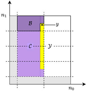
### Visual Description
## Diagram: Set Relationships
### Overview
The image is a diagram illustrating the relationships between sets B and C within a larger space. The diagram uses a coordinate system with axes labeled n0 and n1. The sets B and C are represented by shaded regions, and a vertical yellow bar intersects both sets. A point 'y' is marked at the intersection of the yellow bar and set B.
### Components/Axes
* **Axes:**
* Horizontal axis: n0
* Vertical axis: n1
* **Sets:**
* Set B: Represented by a purple shaded rectangle in the top-left region.
* Set C: Represented by a light purple shaded rectangle below set B.
* **Yellow Bar:** A vertical yellow bar intersecting both sets B and C.
* **Point y:** A black dot labeled 'y' at the intersection of the yellow bar and the top edge of set B.
* **Background:** A grid of dashed lines over a light gray background.
### Detailed Analysis or ### Content Details
* **Set B:** Located in the top-left corner, extending approximately from n0 = 0 to n0 = 0.5 and from n1 = 0.5 to n1 = 1.
* **Set C:** Located below set B, extending approximately from n0 = 0 to n0 = 0.5 and from n1 = 0 to n1 = 0.5.
* **Yellow Bar:** Positioned around n0 = 0.5, extending vertically from approximately n1 = 0 to n1 = 0.75.
* **Point y:** Located at the top of the yellow bar, at approximately n0 = 0.5 and n1 = 0.75.
### Key Observations
* Sets B and C are adjacent, with B above C.
* The yellow bar intersects both sets, indicating a relationship or connection between them.
* Point 'y' marks a specific location within set B, potentially highlighting a key element or boundary.
### Interpretation
The diagram visually represents the spatial relationships between sets B and C. The yellow bar suggests a shared attribute or connection between elements within these sets. Point 'y' could represent a specific element or condition related to both the yellow bar and set B. The diagram likely serves to illustrate a concept or relationship within a mathematical or logical context.
</details>
Figure 8: Definition of Q and L
<details>
<summary>Image 8 Details</summary>
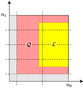
### Visual Description
## Diagram: Set Representation
### Overview
The image is a diagram representing two sets, Q and L, within a larger space defined by axes n0 and n1. The sets are visually distinguished by color (red for Q, yellow for L) and are positioned within a grid-like structure. The diagram illustrates the relationship and overlap between these sets.
### Components/Axes
* **Axes:**
* Horizontal axis: n0
* Vertical axis: n1
* **Sets:**
* Q: Represented by a red area.
* L: Represented by a yellow area.
* **Grid:** Dashed lines forming a grid structure.
* **Background:** Gray area representing the overall space.
### Detailed Analysis
* **Set Q:** The red area representing set Q occupies a significant portion of the space, primarily on the left side. It extends vertically from approximately 0.1 to 1 on the n1 axis and horizontally from approximately 0.1 to 0.6 on the n0 axis.
* **Set L:** The yellow area representing set L is positioned on the right side of the diagram. It extends vertically from approximately 0.3 to 0.9 on the n1 axis and horizontally from approximately 0.6 to 1 on the n0 axis.
* **Overlap:** There is a small region where the red and yellow areas overlap, indicating the intersection of sets Q and L. This overlap occurs approximately between 0.6 and 0.7 on the n0 axis and 0.3 and 0.9 on the n1 axis.
* **Grid:** The dashed grid lines provide a visual reference for the position and extent of the sets. The grid lines are spaced approximately equally along both axes.
### Key Observations
* Sets Q and L have a partial overlap, indicating some common elements.
* Set Q is positioned more towards the left side of the space, while set L is positioned more towards the right.
* The gray background defines the boundaries of the overall space.
### Interpretation
The diagram visually represents the relationship between two sets, Q and L, within a defined space. The overlap between the sets indicates a non-empty intersection, meaning there are elements that belong to both sets. The positioning of the sets relative to the axes and each other provides a spatial understanding of their distribution and relationship within the overall space. The grid helps to visualize the relative sizes and positions of the sets. The diagram is a visual aid to understand set theory concepts.
</details>
This implies that for any choice of P (note that we do not specify a particular choice of P in the proof as long as it has size T ) that rank ' G 2 ' = rank ' G P ' .
Moreover, we do not specify the particular choice of P in the proof, so it holds for all sets of size T .
## D CORRECTNESS OF FASTSECAGG
Correctness essentially follows from the correctness of key agreement and authenticated encryption protocols together with the linearity and D -dropout tolerance of FastShare.
Specifically, using the correctness of key agreement and authenticated encryption, it is straightforward to show that, in Round 2, each client i 2 C 1 computes and sends to the server the sum of shares it receives in Round 1 as follows
<!-- formula-not-decoded -->
«
‹
Figure 9: Showing that B' 0 ; k ' is a subset of the intersection of C and f y ' 0 ; t ' : 0 t k 1 g .
<details>
<summary>Image 9 Details</summary>
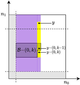
### Visual Description
## Diagram: Illustration of a Region in a 2D Space
### Overview
The image is a diagram illustrating a region within a two-dimensional space defined by axes labeled n0 and n1. The diagram includes several colored regions, points, and labels that define and describe the space.
### Components/Axes
* **Axes:**
* Horizontal axis: Labeled "n0" at the bottom-right.
* Vertical axis: Labeled "n1" at the top-left.
* **Regions:**
* Light gray region: Occupies the bottom and left sides of the diagram, extending to dashed lines.
* Purple region: A rectangular area in the center-left.
* Yellow region: A vertical strip to the right of the purple region.
* Overlapping region: A small area where the purple and yellow regions overlap, resulting in a darker color.
* **Points:**
* Point "y": Located in the upper-right part of the yellow region.
* Point "y-(0, k-1)": Located at the top of the overlapping region.
* Point "y-(0, k)": Located at the bottom of the overlapping region.
* **Labels:**
* "B-(0, k)": Label for the purple region.
### Detailed Analysis
* **Axes:** The axes n0 and n1 define a 2D space. The dashed lines indicate boundaries or limits within this space.
* **Regions:**
* The light gray region seems to represent a background or a broader space.
* The purple region, labeled "B-(0, k)", is a key area of interest. It is a rectangle.
* The yellow region is a vertical strip, possibly representing a specific range or condition along the n0 axis.
* The overlapping region indicates an intersection between the purple and yellow regions.
* **Points:**
* The point "y" is located within the yellow region.
* The points "y-(0, k-1)" and "y-(0, k)" are located at the top and bottom of the overlapping region, respectively. These points seem to be related to the purple region "B-(0, k)".
### Key Observations
* The diagram illustrates the spatial relationships between different regions and points within the n0-n1 space.
* The labels "B-(0, k)", "y-(0, k-1)", and "y-(0, k)" suggest a mathematical or algorithmic context, possibly related to iterative processes or transformations.
### Interpretation
The diagram likely represents a step or state within an iterative process or algorithm. The purple region "B-(0, k)" could represent a set or a state at iteration "k". The yellow region might represent a condition or a filter applied at that iteration. The points "y-(0, k-1)" and "y-(0, k)" could represent the state of "y" before and after applying the condition or filter at iteration "k". The diagram is a visual aid to understand the spatial relationships and transformations occurring within the algorithm.
</details>
Figure 10: Showing that C + ' k ; 0 ' is a subset of the intersection of Q and -k 1 t = 0 'Y + ' t ; 0 '' .
<details>
<summary>Image 10 Details</summary>
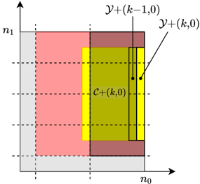
### Visual Description
## Diagram: Overlapping Regions
### Overview
The image is a diagram illustrating overlapping regions in a two-dimensional space, likely representing sets or areas of interest. The diagram uses different colors to distinguish the regions and includes labels to identify them. The axes are labeled as n0 and n1.
### Components/Axes
* **Axes:**
* Horizontal axis: n0
* Vertical axis: n1
* **Regions:**
* Gray region: Located in the bottom-left corner, partially covered by the red region.
* Red region: Overlaps the gray region and extends further towards the top-right.
* Yellow region: Located within the red region, towards the right side.
* Olive region: Overlaps the red and yellow regions, located on the right side.
* **Labels:**
* "y+(k-1,0)": Points to the top edge of the olive region.
* "C+(k,0)": Located within the yellow region.
* "y+(k,0)": Points to the right edge of the olive region.
### Detailed Analysis or ### Content Details
The diagram shows a series of nested and overlapping regions. The gray region is the base, with the red region overlapping it. The yellow region is contained within the red region, and the olive region overlaps both the red and yellow regions. The labels indicate that these regions are likely related to some parameter 'k'.
### Key Observations
* The regions are not perfectly aligned, indicating some degree of variation or change.
* The olive region is the smallest and most specific, located at the intersection of the red and yellow regions.
### Interpretation
The diagram likely represents a concept related to set theory, spatial analysis, or some other field where overlapping regions are used to represent relationships between different entities. The parameter 'k' suggests that this is part of a series or sequence of regions. The overlapping nature of the regions indicates that there are shared characteristics or properties between them. The diagram could be used to illustrate how a particular region (e.g., the olive region) is defined by the intersection of other regions.
</details>
The linearity property of FastShare ensures that the sum of shares is a share of the sum of secret vectors (i.e., client inputs). In other words, by linearity of FastShare, it holds that
<!-- formula-not-decoded -->
Recall that sh ' i denotes the ' -th coefficient of sh i . Therefore, from (43), it holds, for 1 ' d L S e , that
<!-- formula-not-decoded -->
Let C 2 be a random subset of at least N D clients that survive in Round 2, i.e., clients in C 2 send their sum-shares to the server. Now, from (44) and the D -dropout tolerance of FastShare, it holds that FastRecon f' i ; sh ' i 'g i 2C 2 = ˝ j 2C 1 u ' j with probability at least 1 1 poly N for all 1 ' d L S e . Note that we do not need to use a union bound here because if FastRecon succeeds (i.e., does not output ? ) for ' = 1, then it succeeds for each 1 ' d L S e ,
Figure 11: The S is indeed a subset of L . For the particular choice of y this figure shows that the inclusion is true. More generally we in construct S as the intersection of L over all the possible locations of y 2 T .
<details>
<summary>Image 11 Details</summary>
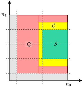
### Visual Description
## Diagram: Set Relationships
### Overview
The image is a diagram illustrating the relationships between three sets: Q, L, and S, within a larger space defined by axes n0 and n1. The diagram uses color-coding to distinguish the sets and their intersections.
### Components/Axes
* **Axes:**
* Horizontal axis: n0
* Vertical axis: n1
* **Sets:**
* Q: Represented by a red area.
* L: Represented by a yellow area.
* S: Represented by a green area.
* **Background:** A gray area represents the space outside the sets.
### Detailed Analysis
* **Set Q (Red):** Occupies a significant portion of the left side of the diagram.
* **Set L (Yellow):** Forms a vertical band on the right side of set Q and above and below set S.
* **Set S (Green):** Located in the intersection of sets Q and L.
* **Intersections:**
* The intersection of Q and L is partially occupied by S.
* The intersection of L and S is the set S.
* **Spatial Relationships:**
* Q is primarily on the left.
* L is primarily on the right.
* S is contained within the intersection of Q and L.
### Key Observations
* The diagram visually represents set inclusion and intersection.
* Set S is a subset of both Q and L.
* The sets are arranged in a way that highlights their overlapping regions.
### Interpretation
The diagram illustrates the relationships between three sets, Q, L, and S, where S is a subset of both Q and L. This type of diagram is commonly used in set theory and logic to visually represent relationships between different groups or categories. The spatial arrangement and color-coding make it easy to understand the inclusion and intersection of these sets. The diagram suggests that elements in set S possess characteristics of both sets Q and L.
</details>
since the locations of missing indices (among N ) of shares for every 1 ' d L S e are the same.
Hence, we get
<!-- formula-not-decoded -->
with probability at least 1 1 poly N . In other words, z = ˝ i 2C 1 u i with probability at least 1 1 poly N . This concludes the proof.
## E SECURITY OF FASTSECAGG
In FastSecAgg, each client i first partitions their input u i to d L S e vectors u 1 i , u 2 i , : : : , u d L S e i , each of length at most S , and computes shares for each u ' , 1 ' d L S e . In other words, we have
i
<!-- formula-not-decoded -->
where independent private randomness is used for each 1 ' d L S e . Let us denote the set of shares that client i generates for client j as » u i … j , i.e., we have
<!-- formula-not-decoded -->
It is straightforward to show that for any set of up to T clients P C , the shares f» u i … j g j 2P reveal no information about u i .
Lemma E.1. For every u i ; v i 2 F L q , for any P C such that jPj T , the distribution of f» u i … j g j 2P is identical to that of f» v i … j g j 2P .
Proof. Here we treat u i to be a random variable (with arbitrary distribution), and f» u i … j g j 2P to be a conditional random variable given a realization of u i . By slightly abusing the notation for simplicity, denote u i as a set u i = f u 1 ; u 2 ; : : : ; u d L S e g (instead of a
i
i
i
vector). Further, for simplicity, define
<!-- formula-not-decoded -->
Now, observe that, given u ' i , the distribution of u ' i P is conditionally independent of u i n f u ' i g and » u i … P n n u ' i P o . This is because, for the ' -th instantiation, 1 ' d L S e , FastShare takes only u ' i as its input and uses independent private randomness. Therefore, the distribution of » u i … P factors into the product of the distributions of u ' i P . The proof then follows by applying the T -privacy property for each instantiation of FastShare.
We prove Theorem 5.2 by a standard hybrid argument. We will present a sequence of hybrids starting that start from the real execution and transition to the simulated execution where each two consecutive hybrids are computationally indistinguishable. Hybrid 0 : This random variable is REAL C ; T ; λ M ' u C ; C 0 ; C 1 ; C 2 ' , the joint view of the parites M in the real execution of the protocol. Hybrid 1 : In this hybrid, we change the behavior of honest clients in C 1 nM so that instead of using KA.agree ' sk i ; pk j ' to encrypt and decrypt messages, we run the key agreement simulator Sim KA ' s i ; j ; pk j ' , where s i ; j is chosen uniformly at random. The security of the key agreement protocol guarantees that this hybrid is indistinguishable from the previous one.
Hybrid 3 : In this hybrid, for every client i 2 C 1 n M , we replace the shares of u i sent to the corrupt clients in M in Round 1 with shares of v i , which are chosen as follows depending on z . If z = ? , then f v i g i 2C 1 nM are chosen uniformly at random. Otherwise, f v i g i 2C 1 nM are chosen uniformly at random subject to ˝ i 2C 1 nM v i = z = ˝ i 2C 1 nM u i . The joint view of corrupt parties contains only jMj T shares of each v i . From Lemma E.1, it follows that this hybrid is identically distributed to the previous one.
Hybrid 2 : In this hybrid, for every client i 2 C 1 n M , we replace the shares of u i sent to other honest clients in Round 1 with zeros, which the adversary observes encrypted as c i ! j . Since only the contents of the ciphertexts are changed, the IND-CPA security of the encryption scheme guarantees that this hybrid is indistinguishable from the previous one.
If z = ? , then we do not need to consider the further hybrids, and let SIM is defined to sample from Hybrid 3 . This distribution can be computed from the inputs z , C 0, and C 1. In the following hybrids, we assume z , ? .
Hybrid 4 : Partition z into d L S e vectors, z 1 , z 2 , : : : , z d L S e , each of length at most S . In this hybrid, for every client i 2 C 2 nM and each 1 ' d L S e , we replace the share sh ' i with the i -th share of z ' + ˝ j 2M u ' j , i.e., h z ' + ˝ j 2M u ' j i . Since z = ˝ i 2C 1 nM u i , from (43)
i and (44), it follows that the distribution of n z + ˝ j 2M u j i o i 2C 2 is identical to that of f sh i g i 2C 2 . Therefore, this hybrid is identically distributed to the previous one.
We define a PPT simulator SIM to sample from the distribution described in the last hybrid. This distribution can be computed from the inputs z , u M , C 0, C 1, and C 2. The argument above proves that
the output of the simulator is computationally indistinguishable from the output of REAL , which concludes the proof.
## F COMPARISON OF FASTSHARE WITH SHAMIR'S SCHEME AND RELATION TO LOCALLY RECOVERABLE CODES
Comparison with the Shamir's scheme: Amulti-secret sharing variant of the Shamir's scheme can be constructed as follows (see, e.g., [16]). We consider the case of generating N shares (each in F q , q N ) from S secrets (each in F q ) such that the privacy threshold is T and dropout tolerance is N S T . Construct a polynomial of degree-' S + T 1 ' with the secrets and T random masks (each in F q ) as coefficients. Its evaluations on N distinct non-zero points in F q yield the N shares for the Shamir's scheme.
Since the shares generated by Shamir are evaluations of a degree-' S + T 1 ' polynomial on N distinct non-zero points, it is easy to see that the shares form a codeword of a Reed-Solomon code of blocklength N and dimension S + T . On the other hand, FastShare constructs a polynomial of degree-' N 1 ' , and evaluates it on primitive N -th roots of unity. The shares generated by FastShare form a codeword of a product code with Reed-Solomon codes as component codes (see Remark 1).
Note that it is possible to recover the secrets from any S + T shares via polynomial interpolation. Although there exist fast polynomial interpolation algorithms that can interpolate a degreen polynomial in O n log 2 n time (see, e.g., [10, 20, 25]), the actual complexity of these algorithms is typically large due to huge constants hidden by the big-Oh notation as noted in [10, 20, 30]. This limits the scalability of such fast interpolation algorithms.
Suppose we choose primitive N -th roots of unity as the evaluation points for the Shamir's multi-secret sharing scheme. Then, the Shamir's scheme essentially computes the Fourier transform of the 'signal' consisting of S secrets, concatenated with T random masks followed by N S T zeros. In contrast, in case of FastShare, we construct the signal by judiciously placing zeros, which ensures the product code structure on the shares.
Relation to LRCs: The variant of FastShare described in 3.4 is related to a class of erasure codes called Locally Recoverable Codes (LRCs) (see [21, 37, 44], and references therein). Specifically, consider LRCs with ' '; r ' locality [37] in which coordinates can be partitioned into several subsets of cardinality ' such that the coordinates in each subset form a maximum distance separable (MDS) code of length ' and dimension r . An efficient construction of such LRCs is presented in [44, Section V-C]. Note that the shares generated by FastShare (as described in 3.4) form codewods of an LRC with ' n 0 ; ' 1 δ 0 ' n 0 ' locality. Moreover, it is not difficult to show that FastShare as an evaluation code is isomorphic to the LRC constructed in [44, Section V-C] when the good polynomial is x ' (see [44, Sections III-A] for the definition of a good polynomial) and the evaluation points are primitive N -th roots of unity.