2102.06455v1

# Deep Sound Field Reconstruction in Real Rooms: Introducing the ISOBEL Sound Field Dataset **Authors**: Miklas Strøm Kristoffersen, Martin Bo Møller, Pablo Martínez-Nuevo, Jan Østergaard ## Deep Sound Field Reconstruction in Real Rooms: Introducing the ISOBEL Sound Field Dataset Miklas Strøm Kristoffersen, 1, 2 Martin Bo Møller, 1 Pablo Mart´ ınez-Nuevo, 1 and Jan Østergaard 2 1 Research Department, Bang & Olufsen a/s, Struer, Denmark 2 AI and Sound Section, Department of Electronic Systems, Aalborg University, Aalborg, Denmark Knowledge of loudspeaker responses are useful in a number of applications, where a sound system is located inside a room that alters the listening experience depending on position within the room. Acquisition of sound fields for sound sources located in reverberant rooms can be achieved through labor intensive measurements of impulse response functions covering the room, or alternatively by means of reconstruction methods which can potentially require significantly fewer measurements. This paper extends evaluations of sound field reconstruction at low frequencies by introducing a dataset with measurements from four real rooms. The ISOBEL Sound Field dataset is publicly available, and aims to bridge the gap between synthetic and real-world sound fields in rectangular rooms. Moreover, the paper advances on a recent deep learning-based method for sound field reconstruction using a very low number of microphones, and proposes an approach for modeling both magnitude and phase response in a U-Net-like neural network architecture. The complex-valued sound field reconstruction demonstrates that the estimated room transfer functions are of high enough accuracy to allow for personalized sound zones with contrast ratios comparable to ideal room transfer functions using 15 microphones below 150 Hz. The following article has been submitted to the Journal of the Acoustical Society of America. After it is published, it will be found at http://asa.scitation.org/journal/jas. ## I. INTRODUCTION The response of a sound system in a room primarily varies with the room itself, the position of the loudspeakers, and the listening position. In order to deliver the intended sound system behavior to listeners, it is necessary to know about and compensate for this effect. Applications include among others room equalization (Cecchi et al. , 2018; Karjalainen et al. , 2001; Radlovic et al. , 2000), virtual reality sound field navigation (Tylka and Choueiri, 2015), source localization (Nowakowski et al. , 2017), and spatial sound field reproduction over predefined or dynamic regions of space also referred to as sound zones (Betlehem et al. , 2015; Møller and Østergaard, 2020). An approach to achieve this, is to measure the loudspeaker response at the desired listening locations and adjust the sound system accordingly. However, the task of measuring impulse responses on a sufficiently fine-grained grid in an entire room, quickly poses as a time-consuming and extensive manual labor that is not desirable. Instead, methods have been developed for the purpose of estimating impulse responses in a room based on a limited number of actual measurements. These methods are also referred to as sound field reconstruction and virtual microphones. The task of reconstructing room impulse responses in positions that have not been measured directly, is an active research field which has been explored in several studies (Ajdler et al. , 2006; Antonello et al. , 2017; Fernandez-Grande, 2019; Mignot et al. , 2014; Verburg and Fernandez-Grande, 2018; Vu and Lissek, 2020). Machine learning, and in particular deep learning, is currently receiving widespread attention across scien- tific domains, and as an example within room acoustics, it has been used to estimate acoustical parameters of rooms (Genovese et al. , 2019; Yu and Kleijn, 2021). In recent work, deep learning-based methods were introduced to sound field reconstruction in reverberant rectangular rooms (Llu´ ıs et al. , 2020). This data-driven approach is able to learn sound field magnitude characteristics from large scale volumes of simulated data without prior information of room characteristics, such as room dimensions and reverberation time. The method is computationally efficient, and works with irregularly and arbitrarily distributed microphones for which there is no requirement of knowing absolute locations in the Euclidean space, in contrast to previous solutions. Furthermore, the reconstruction proves to work with a very low number of microphones, making real-world implementation feasible. To assess the issue of real-world sound field reconstruction, the method is evaluated using measurements in a single room (Llu´ ıs et al. , 2020). However, it is still unknown how much knowledge is transferred from the simulated to the real environment, as well as how well the model generalizes to different real rooms. This is a general problem in deep learning applications that rely on labor intensive data collections, which is our motivation for publishing an open access dataset of real-world sound fields in a diverse set of rooms. This paper studies sound field reconstruction at low frequencies in rectangular rooms with a low number of microphones. The main contributions are: - This paper introduces a sound field dataset, which is publicly available for development and evaluation of sound field reconstruction methods in four real rooms. It is our hope that the ISOBEL Sound Field dataset will help the community in benchmarking and comparing state-of-the-art results. - We assess the real-world performance of deep learning-based sound field magnitude reconstruction trained on simulated sound fields. For this purpose, we consider low frequencies, since lowfrequency room modes can significantly alter listening experience.Furthermore, we are interested in using a very low number of microphones. - Moreover, we extend the deep learning-based sound field reconstruction to cover complex-valued inputs, i.e. both the magnitude and the phase of a sound field. Evaluation is performed in both simulated and real rooms, where a performance gap is observed. We argue why complex sound field reconstruction may have more difficulties in transferring useful knowledge from synthetic to real data. - Lastly, we demonstrate the application of complexvalued sound field reconstruction within the field of sound zone control. Specifically, it is shown that sound fields reconstructed from as little as five microphones pose as valuable inputs to acoustic contrast control. The paper is organized as follows: Section II introduces the concept of sound field reconstruction. Details of measurements from real rooms are presented in Section III. In Section IV, we focus on the problem of reconstructing the magnitude of sound fields, while Section V extends the model to complex-valued sound fields. Finally, Section VI investigates the application of sound zones through sound field reconstruction. ## II. SOUND FIELD RECONSTRUCTION Our approach towards the sound field reconstruction problem is based on the observation that acoustic pressure in a room can be described using a three-dimensional regular grid of points defining a three-dimensional discrete function. The approach specifically for the purpose of magnitude reconstruction was introduced in (Llu´ ıs et al. , 2020). First, let R = [0 , l x ] × [0 , l y ] × [0 , l z ] denote a rectangular room, where l x , l y , l z > 0 are the length, width, and height of the room, respectively. Given such room, we define the grid as a discrete set of coordinates D o . However, for the sake of simplicity, we reduce the three-dimensional problem to a two-dimensional reconstruction on horizontal planes. The two-dimensional grid with a constant height z o is defined as <!-- formula-not-decoded --> for z o ∈ [0 , l z ], i = 0 , . . . , I -1, j = 0 , . . . , J -1, and integers I, J ≥ 2. Note, though, that the dataset collected for this study, which we will introduce in Section III, does in fact contain multiple horizontal planes at different heights. We keep the investigations of three-dimensional reconstruction for future work, and frame the core challenge of this paper as estimation of sound pressure in two-dimensional horizontal planes. The function that we seek to reconstruct on this grid is the Fourier transform of the sound field in a frequency band that covers the low frequencies. The complexvalued frequency-domain sound field calculated using the Fourier transform is given by <!-- formula-not-decoded --> where ω ∈ R is a given excitation frequency, and p ( r , t ) denotes the spatio-temporal sound field with r ∈ R . We refer to the real and imaginary parts of the sound field using s Re ( r , ω ) and s Im ( r , ω ), respectively. Note that s is defined as the magnitude of the Fourier transform in (Llu´ ıs et al. , 2020). Instead, for magnitude reconstruction, we introduce the magnitude of the sound field <!-- formula-not-decoded --> for ω ∈ R and r ∈ R . The procedure for reconstructing s ( r , ω ) on D o takes its starting point from actual observations of the sound field in select positions of the grid. We refer to the collected set of these available sample points as S o , which we further define to be a subset of the full grid. That is, S o ⊆ D o . The cardinality |S o | of the set S o is the number of available sample points, which we will also refer to as the number of microphones n mic in later experiments. We define the samples available to the reconstruction algorithm as <!-- formula-not-decoded --> An important aspect of these definitions is that the grid is unitless and positions can be defined in relative terms. That is, when sampling a point in the grid, only the relative position within the grid, and hence the room, needs to be known. This allows us to relax the data collection compared to alternative methods that require absolute locations. Another important element to consider is that the sampling pattern of S o can form any arrangement within D o as long as 1 ≤ |S o | ≤ |D o | . As an example, this means that sampled points can be irregularly distributed spatially in a room. Situations may arise where the sound field resolution, as defined by l x , I , l y , and J , is too coarse. As an example, consider rooms that are either very long, wide, or in general large. Another example includes applications where fine-grained variations within a sound field are of importance. To compensate for this effect, we allow the reconstruction to base its output on another grid than D o . Such domain will typically be an upsampling of the original grid, but similarly it can be defined with other transformations, e.g. downsampling. Specifically, we define the grid as <!-- formula-not-decoded --> where i = 0 , . . . , IL -1, j = 0 , . . . , J P -1, and L, P must be chosen such that IL, JP ∈ Z + . Note that a value larger than one for either L or P results in an upsampling in the respective dimension. The task of the sound field reconstruction is then to estimate the sound field on the grid D L,P o based on the sampled points S o . In particular, the objective of the reconstruction algorithm is to learn parameters w given <!-- formula-not-decoded --> where g w is an estimator and Ω = { ω k } K k =1 is the set of frequencies at which the sound field will be reconstructed. The remainder of the paper describes the procedure for learning parameters w using deep learning-based methods. ## A. Evaluation Metrics The successfulness of the estimator is quantitatively judged using normalized mean square error (NMSE) at each frequency point in { ω k } K k =1 <!-- formula-not-decoded --> The NMSE provides an average error over all positions in the grid between reconstructed and original sound fields for a single room at a single frequency. We also introduce an average NMSE, which is the NMSE performance averaged over all frequencies of interest as well as over all realizations from M trials, e.g. multiple rooms MNMSE = <!-- formula-not-decoded --> This measure serves as an overall indication of the accuracy of a model, whereas the NMSE k allows a deeper insight of model behaviors at different frequencies. Note that the M trials are specific to each experiment and will be described accordingly. ## III. THE ISOBEL SOUND FIELD DATASET A major contribution of this paper is the ISOBEL Sound Field dataset, which is released as open access alongside the manuscript. 1 The intended purpose is to use the measurements from real rooms for evaluation of sound field reconstruction in a diverse set of rooms. Note that the room-wide measurements of room impulse responses have several other use-cases that will not be further investigated in this paper, but we encourage the use outside sound field reconstruction as well. This section details the dataset and the measurement procedure. 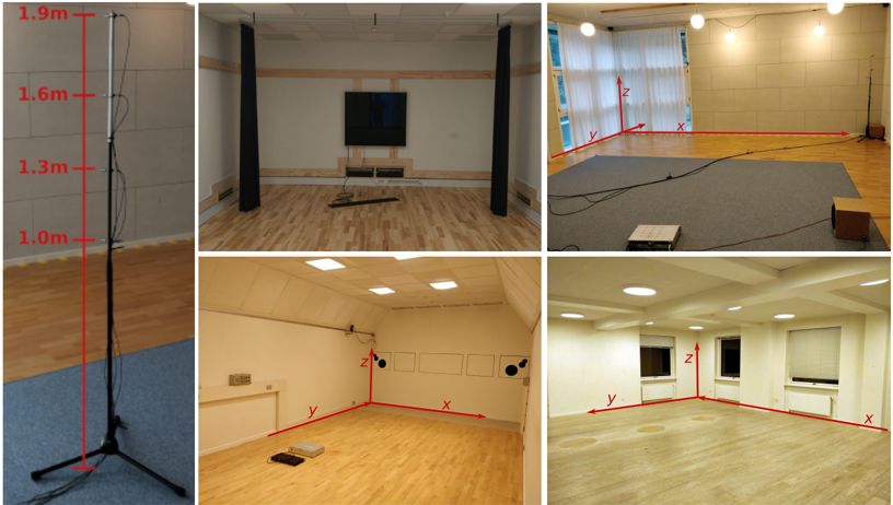The dataset consists of measurements from four different rooms as specified in Table I and depicted in Fig. 1. The data collection is an extension to the real room measured in (Llu´ ıs et al. , 2020), which is included in the ISOBEL Sound Field dataset as Room B for simple access to all measured rooms. The rooms are located at Aalborg University, Aalborg, Denmark, and Bang & Olufsen a/s, Struer, Denmark. The rooms have significantly different acoustic properties and also vary in size. Two types of measurements are conducted in each room: 1) Reverberation time; 2) Sound field. However, only the sound field measurements are released as part of the dataset. The reverberation times are measured in conformity with ISO 3382-2 (ISO 3382-2:2008, 2008) and calculated based on resulting impulse responses using backwards integration and least-squares best fit evaluation of the decay curves. 2 The reverberation times reported in the table are the arithmetic averages of 1/3 octave T 20 estimates in the frequency range 50-316 Hz. The sound field measurements are performed on a 32 by 32 grid with sample points distributed uniformly along the length and width of each room. That is, a total of 1024 positions are measured in each room if possible, but in some cases it is not feasible to measure all positions due to e.g. obstacles. 3 The horizontal grids are measured at four different heights: 1, 1.3, 1.6, and 1.9 meters above the floor. 4 This is achieved using the microphone rig depicted in Fig. 1. Two 10 inch loudspeakers are used to acquire sound fields from two different source positions in each room. Both loudspeakers are placed on the floor, one in a corner and one in an arbitrary position. The sound sources are kept in the same position, while the microphones are moved around the room to record impulse responses. For each microphone position in the grid, the two sources play logarithmic sine sweeps in the frequency range 0.1-24,000 Hz followed by a quiet tail, (Farina, 2000). We use a sampling frequency of 48,000 Hz. The equipment includes among others four G.R.A.S. 40AZ prepolarized free-field microphones connected to four G.R.A.S. 26CC CCP standard preamplifiers and an RME Fireface UFX+ sound card. The four microphones are level calibrated at 1,000 Hz using a Br¨ uel & Kjær sound calibrator type 4231 prior to the measurements. TABLE I. Room characteristics in the ISOBEL Sound Field dataset. The reverberation times are the arithmetic averages of 1/3 octave T 20 estimates in the frequency range 50-316Hz. | Room | Dim. [m] | Size [m 2 /m 3 ] | T 20 [s] | |------------|---------------------|--------------------|------------| | Room B | 4.16 x 6.46 x 2.30 | 27/ 62 | 0.39 | | VR Lab | 6.98 x 8.12 x 3.03 | 57/172 | 0.37 | | List. Room | 4.14 x 7.80 x 2.78 | 32/ 90 | 0.8 | | Prod. Room | 9.13 x 12.03 x 2.60 | 110/286 | 0.77 | FIG. 1. Left: Rig with four microphones. Rooms from top left to bottom right: Room B, VR Lab, Listening Room, and Product Room. <details> <summary>Image 1 Details</summary>  ### Visual Description ## Room Setup Photographs ### Overview The image presents a series of photographs depicting different room setups, likely for acoustic measurements or experiments. The photos showcase various room configurations, equipment placements, and coordinate axes. ### Components/Axes * **Photo 1 (Top Left):** Shows a microphone stand with height markers. * Height markers (from bottom to top): 1.0m, 1.3m, 1.6m, 1.9m. * **Photo 2 (Top Middle):** Shows a room with a TV screen, wooden paneling, and black acoustic panels. * **Photo 3 (Top Right):** Shows a room with a carpeted area, windows with curtains, and coordinate axes. * Coordinate axes: x, y, z. * **Photo 4 (Bottom Left):** Shows a room with acoustic treatment panels on the wall and coordinate axes. * Coordinate axes: x, y, z. * **Photo 5 (Bottom Right):** Shows a room with windows and coordinate axes. * Coordinate axes: x, y, z. ### Detailed Analysis * **Microphone Stand (Photo 1):** A black microphone stand is shown with red lines indicating specific heights. The heights are labeled as 1.0m, 1.3m, 1.6m, and 1.9m. The stand is placed on a blue carpet. * **Room with TV (Photo 2):** The room features a large TV screen mounted on the wall, surrounded by wooden paneling. Two tall, black acoustic panels are positioned on either side of the TV. The floor is made of wooden planks. * **Carpeted Room (Photo 3):** A room with a large gray carpet covering a portion of the floor. Windows with white curtains are visible. Red lines indicate the x, y, and z axes. A microphone stand is visible in the background. * **Acoustically Treated Room (Photo 4):** The room has white walls with several square acoustic panels. Red lines indicate the x, y, and z axes. Some equipment is placed on the floor. * **Room with Windows (Photo 5):** The room has windows with blinds. Red lines indicate the x, y, and z axes. The floor appears to be made of a light-colored material. ### Key Observations * The microphone stand in Photo 1 is used as a reference for height measurements. * Photos 3, 4, and 5 include coordinate axes (x, y, z), suggesting spatial measurements or acoustic analysis. * The rooms in Photos 2 and 4 are treated with acoustic panels, indicating a focus on sound control. ### Interpretation The images likely document different stages or setups of acoustic experiments or measurements in various rooms. The microphone stand provides a height reference, while the coordinate axes in other photos suggest spatial data collection. The presence of acoustic panels indicates a controlled environment for sound-related studies. The different room configurations may be used to analyze how room acoustics affect sound propagation and perception. </details> ## IV. SOUND FIELD MAGNITUDE RECONSTRUCTION In the previous sections we have introduced the problem of reconstructing sound fields on two-dimensional grids in rectangular rooms, as well as introduced a realworld dataset specifically for evaluation of estimators solving such problem. In recent work, (Llu´ ıs et al. , 2020) showed that the problem fits within the context of deep learning-based methods for image reconstruction. Specifically, the tasks of inpainting, (Bertalmio et al. , 2000; Liu et al. , 2018), and super-resolution, (Dong et al. , 2016; Ledig et al. , 2017), which can be paralleled to the tasks of filling in the grid points that are not measured in the sound fields D L,P o \S o , as well as upsampling the grid resolution to achieve fine-grained variations in sound fields. One realization is that these methods are designed to work with real-valued images. To accommodate this, (Llu´ ıs et al. , 2020) propose to reconstruct only the magnitude of the sound field, i.e. | s ( r , ω ) | , using a U-Net-like architecture, (Ronneberger et al. , 2015). To this end, the sampled grids are defined as tensors together with masks specifying which positions are measured (Llu´ ıs et al. , 2020). As an example, {| s ( r , ω k ) |} r ∈D L,P o ,k can be constructed as a tensor of the form S mag ∈ R IL × JP × K . The network is trained using a large number of simulated realizations of rooms, as will be described in the following section. For the experiments, we are interested in assessing the ability of the model to generalize to a wide range of real rooms. ## A. Simulation of Sound Fields for Training Data Green's function can be used to approximate sound fields in rectangular rooms that are lightly damped, (Ja- cobsen and Juhl, 2013). The function provides a solution as an infinite summation of room modes in the three dimensions of a room, x , y , and z . It is defined as follows <!-- formula-not-decoded --> where ∑ N = ∑ ∞ n x =0 ∑ ∞ n y =0 ∑ ∞ n z =0 , for compactness, denotes summation across modal orders in the three dimensions of the room, and similarly the triplet of integers ( n x , n y , n z ) are represented by N . Furthermore, V denotes the volume of the room, ω 2 N represents angular resonance frequency of a mode associated with a specific N , the shape of the mode is denoted ψ N ( · ), τ N is the time constant of the mode, and c is the speed of sound. Assuming rigid boundaries, the shape is determined using the expression (Jacobsen and Juhl, 2013) <!-- formula-not-decoded --> Here, Λ N = √ x y z are constants used for normalization with 0 = 1, 1 = 2 = · · · = 2. Using Sabine's equation, the absorption coefficient is calculated and used to determine time constants of each mode.This is done by assuming that surfaces of a room have uniform distribution of absorption. In the following experiments, two sets of training data are used. The first dataset is introduced in (Llu´ ıs et al. , 2020) and consists of 5,000 rectangular rooms. The room dimensions are sampled randomly in accordance with the recommendations for listening rooms in ITU-R BS.1116-3 (ITU-R BS.1116-3, 2015). The dataset uses a FIG. 2. NMSE in dB of U-Net-based magnitude reconstruction in the four measured rooms with n mic = 15 using the original pretrained model presented in (Llu´ ıs et al. , 2020). <details> <summary>Image 2 Details</summary>  ### Visual Description ## Line Chart: NMSE vs. Frequency for Different Rooms ### Overview The image is a line chart comparing the Normalized Mean Square Error (NMSE) in decibels (dB) across different frequencies for four different rooms: Room B, VR Lab, Listening Room, and Production Room. The chart displays how the NMSE varies with frequency for each room, providing insights into the acoustic characteristics of each space. ### Components/Axes * **X-axis:** Frequency (Hz), ranging from 30 to 300, with tick marks at approximately 30, 40, 50, 60, 70, 80, 90, 100, 200, and 300. * **Y-axis:** NMSE (dB), ranging from -25 to 0, with tick marks at -25, -20, -15, -10, -5, and 0. * **Legend:** Located in the bottom-right corner, identifying each line by room: * Blue: Room B * Green: VR Lab * Black: Listening Room * Red: Production Room ### Detailed Analysis * **Room B (Blue):** * Trend: Starts at approximately -14 dB at 30 Hz, drops sharply to around -16 dB at 42 Hz, then generally increases with frequency, reaching approximately -6 dB at 300 Hz. * Data Points: * 30 Hz: -14 dB * 42 Hz: -16 dB * 60 Hz: -11 dB * 100 Hz: -9 dB * 200 Hz: -8 dB * 300 Hz: -6 dB * **VR Lab (Green):** * Trend: Starts at approximately -9 dB at 30 Hz, drops to -11 dB at 40 Hz, then increases and stabilizes around -4 dB to -6 dB from 80 Hz to 300 Hz. * Data Points: * 30 Hz: -9 dB * 40 Hz: -11 dB * 60 Hz: -8 dB * 100 Hz: -4 dB * 200 Hz: -4 dB * 300 Hz: -6 dB * **Listening Room (Black):** * Trend: Starts at approximately -8 dB at 30 Hz, drops sharply to -16 dB at 42 Hz, then increases and stabilizes around -6 dB to -8 dB from 80 Hz to 300 Hz. * Data Points: * 30 Hz: -8 dB * 42 Hz: -16 dB * 60 Hz: -10 dB * 100 Hz: -7 dB * 200 Hz: -7 dB * 300 Hz: -6 dB * **Production Room (Red):** * Trend: Starts at approximately -6 dB at 30 Hz, remains relatively stable between -5 dB and -7 dB from 30 Hz to 300 Hz, with some fluctuations. * Data Points: * 30 Hz: -6 dB * 60 Hz: -7 dB * 100 Hz: -6 dB * 200 Hz: -6 dB * 300 Hz: -5 dB ### Key Observations * All rooms show a general trend of increasing NMSE with frequency, especially after the initial drop around 40 Hz. * The Production Room exhibits the most stable NMSE across the frequency range. * Room B and Listening Room show a significant dip in NMSE around 40 Hz. * VR Lab has a relatively higher NMSE at lower frequencies compared to Room B and Listening Room after 40 Hz. ### Interpretation The data suggests that the acoustic characteristics of each room vary significantly, especially at lower frequencies. The Production Room appears to have the most consistent performance across the frequency spectrum, indicating a more controlled acoustic environment. The dips in NMSE for Room B and the Listening Room around 40 Hz could indicate specific resonant frequencies or acoustic anomalies in those spaces. The VR Lab's higher NMSE at lower frequencies might be due to the specific design or equipment within that room. Overall, the chart provides valuable insights into the acoustic performance of each room, which could be used to optimize their design or usage for specific audio-related tasks. </details> FIG. 3. NMSE in dB of U-Net-based magnitude reconstruction in the four measured rooms with n mic = 15 using the model presented in (Llu´ ıs et al. , 2020) trained using the extended dataset. <details> <summary>Image 3 Details</summary>  ### Visual Description ## Line Chart: NMSE vs. Frequency for Different Rooms ### Overview The image is a line chart comparing the NMSE (dB) across different frequencies for four different rooms: Room B, VR Lab, Listening Room, and Production Room. The chart shows how the NMSE varies with frequency for each room. ### Components/Axes * **X-axis:** Frequency (Hz), with markers at 30, 40, 50, 60, 70, 80, 90, 100, 200, and 300. * **Y-axis:** NMSE (dB), ranging from -25 to -5, with markers at -25, -20, -15, -10, and -5. * **Legend (bottom-right):** * Blue: Room B * Green: VR Lab * Black: List. Room (Listening Room) * Red: Prod. Room (Production Room) ### Detailed Analysis * **Room B (Blue):** Starts at approximately -15.5 dB at 30 Hz, dips to around -14 dB at 40 Hz, then generally increases to approximately -6 dB at 300 Hz. * **VR Lab (Green):** Starts at approximately -11 dB at 30 Hz, dips to around -12 dB at 40 Hz, then generally increases to approximately -5.5 dB at 300 Hz. * **Listening Room (Black):** Starts at approximately -11 dB at 30 Hz, dips sharply to around -14 dB at 42 Hz, then generally increases to approximately -6 dB at 300 Hz. * **Production Room (Red):** Starts at approximately -9.5 dB at 30 Hz, dips to around -11 dB at 50 Hz, then generally increases to approximately -6 dB at 300 Hz. ### Key Observations * All four rooms show a general trend of increasing NMSE with increasing frequency. * The Listening Room experiences a sharp dip in NMSE around 42 Hz. * The VR Lab generally has a higher NMSE than the other rooms at lower frequencies. * At higher frequencies (around 300 Hz), the NMSE values for all four rooms converge to approximately -6 dB. ### Interpretation The chart illustrates the frequency response characteristics of the four different rooms in terms of NMSE. The general upward trend suggests that NMSE tends to increase with frequency across all rooms. The specific dips and variations in each room's curve indicate unique acoustic properties or measurement artifacts within each environment. The convergence of NMSE values at higher frequencies suggests that the rooms may exhibit similar behavior in that range. The sharp dip in the Listening Room's NMSE around 42 Hz could indicate a resonance or other acoustic phenomenon specific to that room. </details> constant reverberation time T 60 of 0.6 s and only includes room modes in the x and y dimensions, i.e. n z = 0. The second dataset consists of 20,000 rectangular rooms. Room dimensions are uniformly sampled with V ∼ U (50 , 300)m 3 , l x ∼ U (3 . 5 , 10)m, l z ∼ U (1 . 5 , 3 . 5)m, and l y = V/l x l z . Compared to the first dataset, the room dimensions span a larger range and allow us to represent e.g. the Product Room, which is not included in the original training data. The dataset uses reverberation times T 60 sampled from U (0 . 2 , 1 . 0)s and includes room modes in all three x -, y -, and z -dimensions. For both datasets, a grid D L,P o is defined with I = J = 8 and L = P = 4, which effectively divides a sound field into 32x32 uniformly-spaced microphone positions. Using this grid, the magnitude of the sound field is reconstructed at 1/12 octave center-frequencies resolution in the range [30, 300] Hz. Simulations are specified to include all room modes with a resonance frequency below 400 Hz, which means that there is a total of K = 40 frequency slices. ## B. 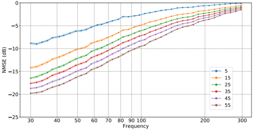Experiments on the ISOBEL Sound Field Dataset The U-Net-like architecture has shown promising results on simulated data and on measurements from a single real room (Llu´ ıs et al. , 2020). In the following experiments, we expose the model to the ISOBEL Sound Field dataset. We include results from the original model, as well as a model built around a similar architecture but using the extended training data with a larger range of room dimensions and reverberation characteristics. We investigate the performance of the model trained with the two different simulated datasets in the four rooms included in the real-world dataset. Special attention is paid to the number of available samples, i.e. the number of microphones n mic . We are mainly interested in settings with a very low number of microphones. In particular, we show results for 5, 15, and 25 microphones in the rooms with a total of 32 × 32 = 1024 available positions. In each room, a total of 40 different and randomly sampled realizations of microphone positions S o are used for each value of n mic . We report the average performance across the 40 realizations, and use the source located in one of the corners of each room. 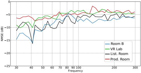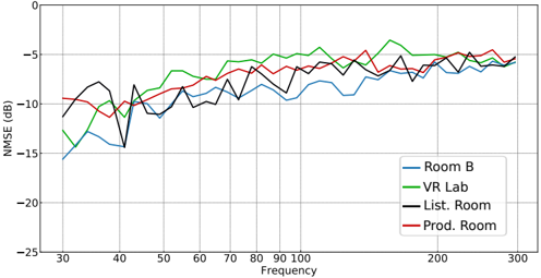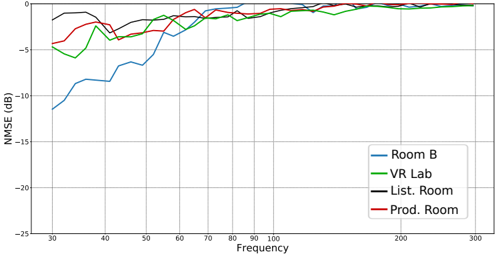Fig. 2 and Fig. 3 show NMSE k results for 15 microphones of model trained with the original and the extended datasets, respectively. It is clear that the model trained with the original dataset does not generalize well to all the rooms. This behavior is expected, since the training data are not designed to represent rooms that fall outside the recommendations for listening room dimensions. On the contrary, the extended training data are motivated in encompassing a wider selection of rooms, which also shows in the results for e.g. the Product Room. One important observation in this regard is that performance does not decrease in rooms that are already represented in the simulated data when more diverse simulated rooms are included, which can e.g. be seen from the performance in Room B. This result indicates that the capacity of the model is sufficient for generalizing to a wide range of diverse rooms and room TABLE II. MNMSE in dB with M = 40 different and randomly sampled realizations of S o for each room in the ISOBEL SF dataset. A lower score is better. | | | n mic | n mic | n mic | |------------|-------|---------|---------|---------| | Room | Model | 5 | 15 | 25 | | Room B | Orig. | -6.33 | -8.71 | -9.62 | | | Ext. | -6.27 | -8.84 | -10.25 | | VR Lab | Orig. | -4.01 | -5.08 | -5.63 | | | Ext. | -4.12 | -6.78 | -8.05 | | List. Room | Orig. | -4.38 | -6.92 | -7.94 | | | Ext. | -5 | -7.61 | -8.44 | | Prod. Room | Orig. | -3.89 | -4.91 | -5.55 | | | Ext. 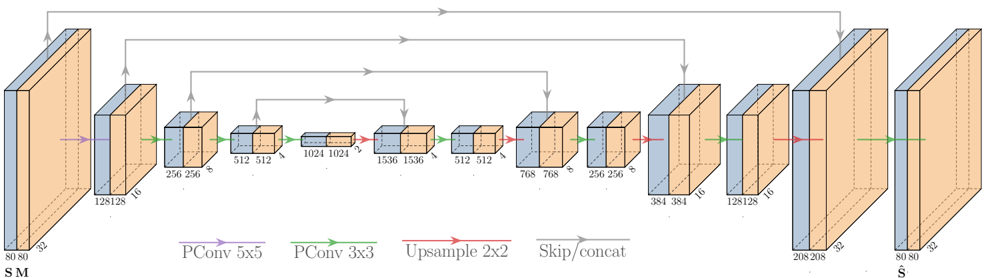| -5.18 | -6.67 | -7.73 | FIG. 4. Architecture of the U-Net-like convolutional neural network proposed for complex sound field reconstruction. S is the tensor with real and imaginary sound fields concatenated along the frequency-dimension, M is the mask tensor, and ˆ S is the reconstructed sound field tensor. <details> <summary>Image 4 Details</summary>  ### Visual Description ## Neural Network Architecture Diagram ### Overview The image is a diagram illustrating the architecture of a neural network, likely an autoencoder or a U-Net variant. It shows the flow of data through different layers, including convolutional layers, upsampling layers, and skip connections. The diagram uses cuboid shapes to represent feature maps, with dimensions indicated below each cuboid. Arrows indicate the direction of data flow and the type of operation performed. ### Components/Axes * **Input:** Labeled "S M" at the bottom-left. Dimensions are 80x80x32. * **Output:** Labeled "Ŝ" at the bottom-right. Dimensions are 80x80x32. * **Layers:** A series of cuboids representing feature maps. Each cuboid is split into two colors, light blue and light orange. * **Arrows:** Indicate data flow and operations. * Purple: PConv 5x5 * Green: PConv 3x3 * Red: Upsample 2x2 * Gray: Skip/concat * **Dimensions:** Numerical values below each cuboid indicate the dimensions of the feature maps. ### Detailed Analysis or ### Content Details **Encoding Path (Left to Right):** 1. **Input:** "S M" with dimensions 80x80x32. 2. **PConv 5x5 (Purple Arrow):** Feature map with dimensions 128x128x16. 3. **PConv 3x3 (Green Arrow):** Feature map with dimensions 256x256x8. 4. **PConv 3x3 (Green Arrow):** Feature map with dimensions 512x512x4. 5. **PConv 3x3 (Green Arrow):** Feature map with dimensions 1024x1024x2. 6. **PConv 3x3 (Green Arrow):** Feature map with dimensions 1536x1536x1. **Decoding Path (Right to Left):** 1. **Upsample 2x2 (Red Arrow):** Feature map with dimensions 512x512x2. 2. **Upsample 2x2 (Red Arrow):** Feature map with dimensions 768x768x4. 3. **Upsample 2x2 (Red Arrow):** Feature map with dimensions 256x256x8. 4. **Upsample 2x2 (Red Arrow):** Feature map with dimensions 384x384x16. 5. **PConv 3x3 (Green Arrow):** Feature map with dimensions 128x128x16. 6. **PConv 3x3 (Green Arrow):** Feature map with dimensions 208x208x32. 7. **PConv 3x3 (Green Arrow):** Output "Ŝ" with dimensions 80x80x32. **Skip Connections (Gray Arrows):** * From 128x128x16 to 128x128x16 * From 256x256x8 to 256x256x8 * From 512x512x4 to 512x512x2 * From 1536x1536x1 to 768x768x4 ### Key Observations * The diagram illustrates a U-Net-like architecture with skip connections. * The encoding path progressively reduces the spatial dimensions while increasing the number of channels. * The decoding path progressively increases the spatial dimensions while decreasing the number of channels. * Skip connections are used to concatenate feature maps from the encoding path to the decoding path, likely to preserve fine-grained details. * The dimensions of the feature maps are explicitly stated, providing a clear understanding of the network's structure. ### Interpretation The diagram represents a neural network architecture designed for tasks such as image segmentation or image-to-image translation. The U-Net structure with skip connections allows the network to capture both high-level contextual information and low-level details. The specific dimensions and operations (PConv, Upsample) suggest a tailored design for a particular application. The skip connections are crucial for transferring information from earlier layers to later layers, which helps to improve the accuracy and detail of the output. The consistent use of PConv layers indicates a focus on learning local features. </details> acoustic characteristics, given that the model is provided with ample training samples. Table II details MNMSE results, which are the NMSE results averaged across frequencies K = 40 and S o realizations M = 40. The MNMSE results for n mic = 15 are the condensed results shown for the NMSE k in Figs. 2 and 3. The scores in the table reiterate the observations from the figures, performance is improved with the extended training data for some rooms in particular, while performance is maintained in the other rooms. Interestingly, there seems to be a tendency of more pronounced improvements with a larger number of microphones. We attribute this effect to similar observations within classical methods that as the number of microphones increase, relative improvement for reconstruction is higher at low frequencies as opposed to the highfrequency range, (Ajdler et al. , 2006; Llu´ ıs et al. , 2020). In summary, the deep learning-based model is confirmed to possess the ability to generalize to a diverse set of real rooms for sound field magnitude reconstruction. Based solely on training with simulated data, these promising results motivate further investigations, e.g. of reconstructing the complex-valued sound fields. ## V. COMPLEX SOUND FIELD RECONSTRUCTION We propose to extend the U-Net-based model to work with complex-valued room transfer functions (RTFs). Reconstruction of both magnitude and phase of sound fields enable new opportunities, such as the application of sound zones. A topic, which we investigate in Section VI. The proposed model is based on the model designed to work with the magnitude of sound fields. Note that deep learning-based models that work directly on complex-valued inputs have been introduced, e.g. within Transformers (Kim et al. , 2020; Yang et al. , 2020), but in this paper we instead choose to process the sound fields such that the U-Net-based model receives real-valued inputs. Specifically, we present the model to real and imaginary parts of sound fields separately. That is, where the magnitude-based model receive as input {| s ( r , ω k ) |} r ∈D L,P o ,k in the tensor form S mag ∈ R IL × JP × K , the complex-based model instead receives a concatenation of the real and imaginary sound fields. Specifically, using the real sound field { s Re ( r , ω k ) } r ∈D L,P o ,k with the tensor form S Re ∈ R IL × JP × K , and similarly the imaginary sound field tensor S Im ∈ R IL × JP × K , we define the concatenated input: <!-- formula-not-decoded --> where S ∈ R IL × JP × 2 K is the resulting tensor with real and imaginary sound fields concatenated along the frequency-dimension. Note that the complex-valued sound field is easily recovered from this tensor form. In addition, we define a mask tensor M ∈ R IL × JP × 2 K computed from S o and D L,P o . We follow the pre- and postprocessing steps as described in (Llu´ ıs et al. , 2020), which entails completion, scaling, upsampling, mask generation, and rescaling based on linear regression. These steps are, however, adjusted such that they operate on a tensor that has doubled in size from K to 2 K in the third dimension. Furthermore, we have observed significant improvements by changing the min-max scaling of the input to a max scaling that takes into account both real and imaginary parts for each frequency slice. Specifically: <!-- formula-not-decoded --> <!-- formula-not-decoded --> for each ω k . Note that this alters the scaling operation from working in the range [0,1] to working in [-1,1]. The motivation in doing so, is that values can be negative, in contrast to the real values from the magnitude. By using max scaling we ensure that zero will not shift between realizations. The architecture of the proposed neural network, as illustrated in Fig. 4, is based on a U-Net (Ronneberger et al. , 2015). We employ partial convolutions (PConv) as proposed for image inpainting in (Liu et al. , 2018). In the encoding part of the U-Net, we use a stride of two in the partial convolutions in order to halve the feature maps, while doubling the number of kernels in each layer. The decoder part acts opposite with upsampling feature maps and reducing the number of kernels to reach an output tensor ˆ S with matching dimensions to the input tensor S . We use ReLU as activation function in the encoding part, and leaky ReLU with a slope coefficient of -0.2 in the decoder. We initialize the weights using the uniform Xavier method (Glorot and Bengio, 2010), initialize the biases as zero, and use the Adam optimizer (Kingma and Ba, 2014) with early stopping when performance on a validation set stops increasing. Due to the increased input and output sizes, we double the number of kernels in all layers compared to the U-Net for magnitude reconstruction. We also do not use a 1x1 convolution with sigmoid activation in the last layer, since the range of our output is not constrained to [0,1] but instead [-1,1]. We have not experienced any decreases in performance from not including this layer. ## A. Experiments In this section, we assess the complex-valued sound field reconstruction. The simulated extended dataset introduced in Section IV A is used to train the model. It is important to note that NMSE scores are not directly comparable between magnitude and complex reconstruction, for which reason it is not possible to scrutinize differences between the two types of models. That is, the results presented in the following experiments will stand on their own, and only indicative parallels can be drawn to the results from magnitude reconstruction. First, we test how the model performs on the simulated data associated with the training data, but held out specifically for evaluation. This test set consists of 190 simulated rooms, the validation set contains approximately 1,000 rooms, and the training set holds the remaining rooms from the 20,000 available rooms. In each room, three different realizations of S o are used for each value of n mic . Results in terms of NMSE are shown in Fig. 5. Some tendencies are similar to those observed for magnitude reconstruction, such as improvements in performance with an increasing number of available microphones. At the same time, as frequency increases, performance degrades. Next, we evaluate the complex reconstruction model on the ISOBEL Sound Field dataset. The approach is similar to the experiment in Section IV B, except the use of the complex-valued sound fields instead of the magnitude. As can be seen from the results in Fig. 6, per- FIG. 5. NMSE in dB for complex reconstruction of simulated sound fields in the test set with 190 different rooms and three realizations of S o in each room ( M = 570 for each value of n mic ). The solid lines indicate average NMSE k shown with 95% confidence intervals. Colors indicate different values of n mic in the range [5, 55]. <details> <summary>Image 5 Details</summary>  ### Visual Description ## Line Chart: NMSE vs. Frequency for Different Parameters ### Overview The image is a line chart showing the relationship between NMSE (Normalized Mean Squared Error) in dB and Frequency. There are six different lines, each representing a different parameter value (5, 15, 25, 35, 45, and 55). The chart illustrates how NMSE changes with frequency for each parameter. ### Components/Axes * **X-axis:** Frequency, ranging from approximately 30 to 300. Major tick marks are present at 30, 40, 50, 60, 70, 80, 90, 100, 200, and 300. * **Y-axis:** NMSE (dB), ranging from -25 to 0. Major tick marks are present at -25, -20, -15, -10, -5, and 0. * **Legend:** Located in the bottom-right corner. It identifies each line by its parameter value: * Blue: 5 * Orange: 15 * Green: 25 * Red: 35 * Purple: 45 * Brown: 55 ### Detailed Analysis * **Blue Line (5):** The NMSE starts at approximately -9 dB at a frequency of 30, then increases steadily to approximately -2 dB at a frequency of 300. * **Orange Line (15):** The NMSE starts at approximately -14 dB at a frequency of 30, then increases steadily to approximately -3 dB at a frequency of 300. * **Green Line (25):** The NMSE starts at approximately -16 dB at a frequency of 30, then increases steadily to approximately -4 dB at a frequency of 300. * **Red Line (35):** The NMSE starts at approximately -17 dB at a frequency of 30, then increases steadily to approximately -4.5 dB at a frequency of 300. * **Purple Line (45):** The NMSE starts at approximately -18 dB at a frequency of 30, then increases steadily to approximately -5 dB at a frequency of 300. * **Brown Line (55):** The NMSE starts at approximately -19 dB at a frequency of 30, then increases steadily to approximately -5.5 dB at a frequency of 300. ### Key Observations * All lines show an upward trend, indicating that NMSE increases with frequency. * The lines are generally parallel, suggesting a similar relationship between NMSE and frequency for all parameter values. * The NMSE values are lower for higher parameter values across the frequency range. * The rate of increase in NMSE decreases as frequency increases, with the lines appearing to flatten out towards the higher end of the frequency range. ### Interpretation The chart demonstrates the relationship between NMSE and frequency for different parameter values. The data suggests that increasing the frequency generally leads to a higher NMSE, regardless of the parameter value. However, higher parameter values result in lower NMSE across the frequency spectrum. The convergence of the lines at higher frequencies suggests that the impact of the parameter value on NMSE diminishes as frequency increases. This information could be valuable in optimizing system parameters to minimize NMSE at different operating frequencies. </details> FIG. 6. Average NMSE k in dB of complex reconstruction in the four measured rooms with n mic = 15. <details> <summary>Image 6 Details</summary>  ### Visual Description ## Line Chart: NMSE vs. Frequency for Different Rooms ### Overview The image is a line chart comparing the Normalized Mean Square Error (NMSE) in decibels (dB) against frequency for four different rooms: Room B, VR Lab, Listening Room, and Production Room. The chart shows how the NMSE changes with frequency for each room. ### Components/Axes * **X-axis:** Frequency, ranging from 30 to 300. Axis markers are present at approximately 30, 40, 50, 60, 70, 80, 90, 100, 200, and 300. * **Y-axis:** NMSE (dB), ranging from -25 to 0. Axis markers are present at 0, -5, -10, -15, -20, and -25. * **Legend:** Located in the bottom-right corner, identifying the lines by color: * Blue: Room B * Green: VR Lab * Black: List. Room (Listening Room) * Red: Prod. Room (Production Room) ### Detailed Analysis * **Room B (Blue):** The NMSE starts at approximately -11 dB at 30 Hz, increases sharply to about -8 dB at 40 Hz, then to -7 dB at 50 Hz, and then increases more gradually to approximately -2 dB at 70 Hz. It then plateaus around -1 dB to 0 dB from 80 Hz to 300 Hz. * **VR Lab (Green):** The NMSE starts at approximately -5 dB at 30 Hz, decreases to about -6 dB at 35 Hz, then increases to approximately -3 dB at 60 Hz. It then plateaus around -2 dB to 0 dB from 70 Hz to 300 Hz. * **Listening Room (Black):** The NMSE starts at approximately -2 dB at 30 Hz, decreases slightly to about -3 dB at 40 Hz, then increases to approximately -1 dB at 60 Hz. It then plateaus around -1 dB to 0 dB from 70 Hz to 300 Hz. * **Production Room (Red):** The NMSE starts at approximately -4 dB at 30 Hz, decreases slightly to about -4.5 dB at 40 Hz, then increases to approximately -1 dB at 60 Hz. It then plateaus around -1 dB to 0 dB from 70 Hz to 300 Hz. ### Key Observations * All rooms show a general trend of increasing NMSE with frequency up to around 70 Hz. * After 70 Hz, the NMSE for all rooms plateaus and remains relatively constant. * Room B has the lowest NMSE at lower frequencies (30-60 Hz) but catches up with the other rooms at higher frequencies. * The Listening Room and Production Room have very similar NMSE values across the entire frequency range. ### Interpretation The chart suggests that the acoustic performance, as measured by NMSE, improves with increasing frequency for all rooms, up to a certain point (around 70 Hz). After this point, the NMSE stabilizes, indicating that the rooms' acoustic characteristics become more consistent across higher frequencies. Room B exhibits a poorer performance at lower frequencies compared to the other rooms, potentially indicating issues with low-frequency response or noise. The similarity between the Listening Room and Production Room suggests they have similar acoustic properties, possibly due to similar design or treatment. The data could be used to identify frequency ranges where specific rooms require acoustic treatment or modifications to improve their performance. </details> formances in the real rooms are not comparable to those from simulated data. Moreover, although it is not possible to compare directly, performance seems worse than what is achieved with the magnitude-based reconstruction in the same rooms, see Fig. 3. That is, the complex reconstruction model is not transferring useful knowledge as successfully from the simulations-based training to the real world. Given that the network is able to reconstruct the simulated sound fields, it appears that the complex simulation model is a worse match for the real rooms than the magnitude simulation model. The outcome is that the framework is able to reconstruct sound fields which are close to fields included in the training data, it is indicated that the complex simulations are a poor match for the real rooms. Two apparent differences are the identical boundary conditions at all surfaces and perfectly rectangular geometry assumed in the simulations, but which are not true in the real rooms. To provide insights into how the network behaves relative to rooms which does not match the training data set we now present the following simulations. FIG. 7. NMSE in dB for complex reconstruction of simulated sound fields in rooms with no or small variations in the room dimensions. Rows: Training data. Columns: Test data. Four random realizations of S o are used in each of the 11 test rooms ( M = 44). The solid lines indicate average NMSE k shown with 95% confidence intervals. Colors indicate different n mic values, i.e., n mic = 5 (blue), n mic = 15 (orange), n mic = 25 (green), n mic = 35 (red), n mic = 45 (purple), and n mic = 55 (brown). <details> <summary>Image 7 Details</summary>  ### Visual Description ## Chart Type: NMSE vs. Frequency for Simulated List. Room ### Overview The image presents a series of line graphs arranged in a 3x3 grid. Each graph displays the Normalized Mean Square Error (NMSE) in dB as a function of frequency for a simulated listening room. The rows represent different spatial perturbations applied to the listening room's location, while the columns represent different training conditions. Each graph contains multiple lines, each representing a different number of training samples (5, 15, 25, 35, 45, 55). The shaded regions around each line indicate uncertainty. ### Components/Axes * **Title:** "Simulated List. Room" (with variations for spatial perturbation) * **X-axis:** Frequency (Hz), with markers at approximately 30, 40, 50, 60, 70, 80, 90, 100, 200, and 300. * **Y-axis:** NMSE (dB), with markers at 0, -5, -10, -15, -20, and -25. * **Legend:** Located in the top-left graph, indicating the number of training samples: * Blue: 5 * Green: 15 * Red: 25 * Yellow: 35 * Purple: 45 * Brown: 55 * **Spatial Perturbations (Rows):** * Row 1: "Simulated List. Room" * Row 2: "Simulated List. Room lx + U(-0.25, 0.25)m" * Row 3: "Simulated List. Room lx + U(-1.0, 1.0)m" * **Training Conditions (Columns):** * Column 1: Training condition not explicitly stated on the graph, but implied to be the base condition. * Column 2: "lx + U(-0.25, 0.25)m" * Column 3: "lx + U(-1.0, 1.0)m" * **Diagram Note:** In the top left of the image, there is a diagram with "Test ->" and "Train ↓" indicating the direction of testing and training. ### Detailed Analysis **Row 1: Simulated List. Room** * **Column 1:** * Blue (5): Starts at approximately -23 dB at 30 Hz, rises sharply to about -12 dB at 50 Hz, fluctuates, and then gradually increases to about -5 dB at 300 Hz. * Green (15): Starts at approximately -23 dB at 30 Hz, rises sharply to about -12 dB at 50 Hz, fluctuates, and then gradually increases to about -5 dB at 300 Hz. * Red (25): Starts at approximately -23 dB at 30 Hz, rises sharply to about -12 dB at 50 Hz, fluctuates, and then gradually increases to about -5 dB at 300 Hz. * Yellow (35): Starts at approximately -23 dB at 30 Hz, rises sharply to about -12 dB at 50 Hz, fluctuates, and then gradually increases to about -5 dB at 300 Hz. * Purple (45): Starts at approximately -23 dB at 30 Hz, rises sharply to about -12 dB at 50 Hz, fluctuates, and then gradually increases to about -5 dB at 300 Hz. * Brown (55): Starts at approximately -23 dB at 30 Hz, rises sharply to about -12 dB at 50 Hz, fluctuates, and then gradually increases to about -5 dB at 300 Hz. * **Column 2:** * Blue (5): Starts at approximately -23 dB at 30 Hz, rises sharply to about -10 dB at 50 Hz, fluctuates, and then gradually increases to about -4 dB at 300 Hz. * Green (15): Starts at approximately -23 dB at 30 Hz, rises sharply to about -10 dB at 50 Hz, fluctuates, and then gradually increases to about -4 dB at 300 Hz. * Red (25): Starts at approximately -23 dB at 30 Hz, rises sharply to about -10 dB at 50 Hz, fluctuates, and then gradually increases to about -4 dB at 300 Hz. * Yellow (35): Starts at approximately -23 dB at 30 Hz, rises sharply to about -10 dB at 50 Hz, fluctuates, and then gradually increases to about -4 dB at 300 Hz. * Purple (45): Starts at approximately -23 dB at 30 Hz, rises sharply to about -10 dB at 50 Hz, fluctuates, and then gradually increases to about -4 dB at 300 Hz. * Brown (55): Starts at approximately -23 dB at 30 Hz, rises sharply to about -10 dB at 50 Hz, fluctuates, and then gradually increases to about -4 dB at 300 Hz. * **Column 3:** * Blue (5): Starts at approximately -23 dB at 30 Hz, rises sharply to about -5 dB at 50 Hz, fluctuates, and then gradually increases to about -3 dB at 300 Hz. * Green (15): Starts at approximately -23 dB at 30 Hz, rises sharply to about -5 dB at 50 Hz, fluctuates, and then gradually increases to about -3 dB at 300 Hz. * Red (25): Starts at approximately -23 dB at 30 Hz, rises sharply to about -5 dB at 50 Hz, fluctuates, and then gradually increases to about -3 dB at 300 Hz. * Yellow (35): Starts at approximately -23 dB at 30 Hz, rises sharply to about -5 dB at 50 Hz, fluctuates, and then gradually increases to about -3 dB at 300 Hz. * Purple (45): Starts at approximately -23 dB at 30 Hz, rises sharply to about -5 dB at 50 Hz, fluctuates, and then gradually increases to about -3 dB at 300 Hz. * Brown (55): Starts at approximately -23 dB at 30 Hz, rises sharply to about -5 dB at 50 Hz, fluctuates, and then gradually increases to about -3 dB at 300 Hz. **Row 2: Simulated List. Room lx + U(-0.25, 0.25)m** * **Column 1:** * Blue (5): Starts at approximately -20 dB at 30 Hz, rises sharply to about -8 dB at 50 Hz, fluctuates, and then gradually increases to about -4 dB at 300 Hz. * Green (15): Starts at approximately -20 dB at 30 Hz, rises sharply to about -8 dB at 50 Hz, fluctuates, and then gradually increases to about -4 dB at 300 Hz. * Red (25): Starts at approximately -20 dB at 30 Hz, rises sharply to about -8 dB at 50 Hz, fluctuates, and then gradually increases to about -4 dB at 300 Hz. * Yellow (35): Starts at approximately -20 dB at 30 Hz, rises sharply to about -8 dB at 50 Hz, fluctuates, and then gradually increases to about -4 dB at 300 Hz. * Purple (45): Starts at approximately -20 dB at 30 Hz, rises sharply to about -8 dB at 50 Hz, fluctuates, and then gradually increases to about -4 dB at 300 Hz. * Brown (55): Starts at approximately -20 dB at 30 Hz, rises sharply to about -8 dB at 50 Hz, fluctuates, and then gradually increases to about -4 dB at 300 Hz. * **Column 2:** * Blue (5): Starts at approximately -20 dB at 30 Hz, rises sharply to about -8 dB at 50 Hz, fluctuates, and then gradually increases to about -4 dB at 300 Hz. * Green (15): Starts at approximately -20 dB at 30 Hz, rises sharply to about -8 dB at 50 Hz, fluctuates, and then gradually increases to about -4 dB at 300 Hz. * Red (25): Starts at approximately -20 dB at 30 Hz, rises sharply to about -8 dB at 50 Hz, fluctuates, and then gradually increases to about -4 dB at 300 Hz. * Yellow (35): Starts at approximately -20 dB at 30 Hz, rises sharply to about -8 dB at 50 Hz, fluctuates, and then gradually increases to about -4 dB at 300 Hz. * Purple (45): Starts at approximately -20 dB at 30 Hz, rises sharply to about -8 dB at 50 Hz, fluctuates, and then gradually increases to about -4 dB at 300 Hz. * Brown (55): Starts at approximately -20 dB at 30 Hz, rises sharply to about -8 dB at 50 Hz, fluctuates, and then gradually increases to about -4 dB at 300 Hz. * **Column 3:** * Blue (5): Starts at approximately -20 dB at 30 Hz, rises sharply to about -8 dB at 50 Hz, fluctuates, and then gradually increases to about -4 dB at 300 Hz. * Green (15): Starts at approximately -20 dB at 30 Hz, rises sharply to about -8 dB at 50 Hz, fluctuates, and then gradually increases to about -4 dB at 300 Hz. * Red (25): Starts at approximately -20 dB at 30 Hz, rises sharply to about -8 dB at 50 Hz, fluctuates, and then gradually increases to about -4 dB at 300 Hz. * Yellow (35): Starts at approximately -20 dB at 30 Hz, rises sharply to about -8 dB at 50 Hz, fluctuates, and then gradually increases to about -4 dB at 300 Hz. * Purple (45): Starts at approximately -20 dB at 30 Hz, rises sharply to about -8 dB at 50 Hz, fluctuates, and then gradually increases to about -4 dB at 300 Hz. * Brown (55): Starts at approximately -20 dB at 30 Hz, rises sharply to about -8 dB at 50 Hz, fluctuates, and then gradually increases to about -4 dB at 300 Hz. **Row 3: Simulated List. Room lx + U(-1.0, 1.0)m** * **Column 1:** * Blue (5): Starts at approximately -20 dB at 30 Hz, rises sharply to about -8 dB at 50 Hz, fluctuates, and then gradually increases to about -4 dB at 300 Hz. * Green (15): Starts at approximately -20 dB at 30 Hz, rises sharply to about -8 dB at 50 Hz, fluctuates, and then gradually increases to about -4 dB at 300 Hz. * Red (25): Starts at approximately -20 dB at 30 Hz, rises sharply to about -8 dB at 50 Hz, fluctuates, and then gradually increases to about -4 dB at 300 Hz. * Yellow (35): Starts at approximately -20 dB at 30 Hz, rises sharply to about -8 dB at 50 Hz, fluctuates, and then gradually increases to about -4 dB at 300 Hz. * Purple (45): Starts at approximately -20 dB at 30 Hz, rises sharply to about -8 dB at 50 Hz, fluctuates, and then gradually increases to about -4 dB at 300 Hz. * Brown (55): Starts at approximately -20 dB at 30 Hz, rises sharply to about -8 dB at 50 Hz, fluctuates, and then gradually increases to about -4 dB at 300 Hz. * **Column 2:** * Blue (5): Starts at approximately -20 dB at 30 Hz, rises sharply to about -8 dB at 50 Hz, fluctuates, and then gradually increases to about -4 dB at 300 Hz. * Green (15): Starts at approximately -20 dB at 30 Hz, rises sharply to about -8 dB at 50 Hz, fluctuates, and then gradually increases to about -4 dB at 300 Hz. * Red (25): Starts at approximately -20 dB at 30 Hz, rises sharply to about -8 dB at 50 Hz, fluctuates, and then gradually increases to about -4 dB at 300 Hz. * Yellow (35): Starts at approximately -20 dB at 30 Hz, rises sharply to about -8 dB at 50 Hz, fluctuates, and then gradually increases to about -4 dB at 300 Hz. * Purple (45): Starts at approximately -20 dB at 30 Hz, rises sharply to about -8 dB at 50 Hz, fluctuates, and then gradually increases to about -4 dB at 300 Hz. * Brown (55): Starts at approximately -20 dB at 30 Hz, rises sharply to about -8 dB at 50 Hz, fluctuates, and then gradually increases to about -4 dB at 300 Hz. * **Column 3:** * Blue (5): Starts at approximately -20 dB at 30 Hz, rises sharply to about -8 dB at 50 Hz, fluctuates, and then gradually increases to about -4 dB at 300 Hz. * Green (15): Starts at approximately -20 dB at 30 Hz, rises sharply to about -8 dB at 50 Hz, fluctuates, and then gradually increases to about -4 dB at 300 Hz. * Red (25): Starts at approximately -20 dB at 30 Hz, rises sharply to about -8 dB at 50 Hz, fluctuates, and then gradually increases to about -4 dB at 300 Hz. * Yellow (35): Starts at approximately -20 dB at 30 Hz, rises sharply to about -8 dB at 50 Hz, fluctuates, and then gradually increases to about -4 dB at 300 Hz. * Purple (45): Starts at approximately -20 dB at 30 Hz, rises sharply to about -8 dB at 50 Hz, fluctuates, and then gradually increases to about -4 dB at 300 Hz. * Brown (55): Starts at approximately -20 dB at 30 Hz, rises sharply to about -8 dB at 50 Hz, fluctuates, and then gradually increases to about -4 dB at 300 Hz. ### Key Observations * The NMSE generally decreases (improves) as the frequency increases. * Increasing the number of training samples (from 5 to 55) generally leads to a slight decrease in NMSE, but the effect is not dramatic. The lines are very close together. * The spatial perturbation "lx + U(-1.0, 1.0)m" generally results in a slightly lower NMSE compared to "lx + U(-0.25, 0.25)m" and the base "Simulated List. Room" condition. * There are noticeable fluctuations in NMSE across the frequency range, indicating resonances or other acoustic phenomena within the simulated room. ### Interpretation The data suggests that increasing the number of training samples has a limited impact on the NMSE for this particular simulated listening room scenario. The spatial perturbation of the listening room's location appears to have a more significant effect, with larger perturbations (U(-1.0, 1.0)m) leading to slightly better performance. The fluctuations in NMSE across the frequency range highlight the importance of considering the acoustic characteristics of the room when evaluating the performance of a system. The "Test ->" and "Train ↓" diagram suggests that the training and testing data are generated using different methods or conditions, which could explain the need for spatial perturbation to improve generalization. The U(-0.25, 0.25)m and U(-1.0, 1.0)m likely represent a uniform distribution of spatial offsets. </details> ## B. 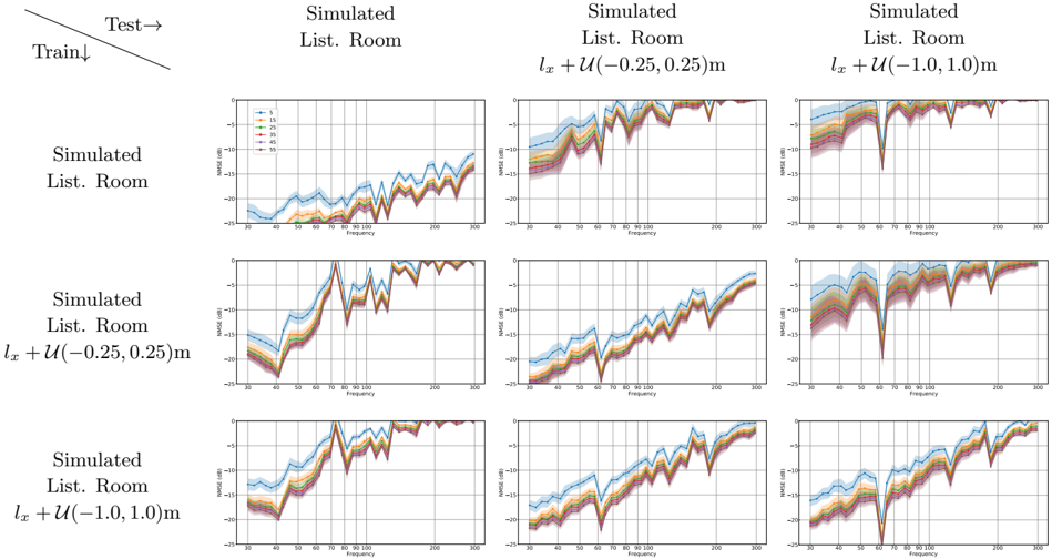Discussion of Experiments Several optimizations and fine-tuning approaches have been investigated for the complex reconstruction in real rooms without achieving notable improvements. Instead, we take another approach, and show what happens to the model, when it is exposed to data that are not represented in the training data. To this end, we are interested in assessing the performance of room specialized models. That is, if room dimensions and reverberation time are known, how well will a model trained specifically for that room perform. For this, we introduce new datasets each with 824 realizations for training, 165 for validation, and 11 for testing. Each simulated realization has a randomly positioned source. In total, three such datasets are generated according to the procedure described in Section IV A. The first dataset assumes that room characteristics are known perfectly, we use the parameters of the Listening Room. The second and third datasets introduce uncertainty in the room dimensions. In particular, we alter the length and width of rooms, while keeping the aspect ratio ( l x /l y ) of the room constant. We accomplish this by uniformly sampling an error, which is added to the length of a room, and correct the width to achieve the original aspect ratio. The two datasets sample errors in the range [-0.25, 0.25] m and [-1, 1] m, respectively. The results for the three models evaluated on each of the test sets are shown in Fig. 7. The first column shows how the three models perform on the dataset with no added uncertainties. Even with small variations of the 0.25 m scale, performance rapidly degrades with increasing frequency. On the diagonal, training data match test data, and once again high frequencies see a significant performance decrease with increasing uncertainty. In general, the models do not perform well on datasets with more variation than what is included in their own training data, which can be seen in the three upper right figures. Further experiments showed that the three models do not generalize to the real-world measurements of the Listening Room. This result indicates that the simplifications imposed during the simulations of rooms causes the simulated sound fields to not represent the exact real rooms we intend it to. That is, a model trained with simulated data generated using exact parameters of a real room will not be able to reconstruct the sound field accurately in the real room. As suggested by our results, neither will a model trained with ± 1 m uncertainty. This calls for inclusion of diverse room parameters when training a model with simulated data if the intended purpose is to use the reconstruction in real rooms. We showed in Section IV how magnitude reconstruction recovered performance in some of the real rooms by using an extended training dataset with more diverse simulated rooms. The same effect is not observed for complex reconstruction. We believe two factors are the main reasons: 1) the boundary conditions in the simulations assume nearly rigid walls and do not include e.g. phase shifts of real wall reflections; 2) the simulations assume perfectly rectangular rooms with a uniform dis- tribution of absorption. Thus, we hypothesize that the model does not see representative data during training, analogous to not having the correct room dimensions represented in the training data. ## VI. THE SOUND ZONES APPLICATION One potential application for the sound field reconstruction presented in this paper, is in the process of setting up sound zones. Sound zones generally refers to the scenario where multiple loudspeakers are used to reproduce individual audio signals to individual people within a room (Betlehem et al. , 2015). To control the sound field at the location of the listeners in the room, it is necessary to know the RTFs between each loudspeaker and locations sampling the listening regions. If the desired locations of the sound zones change over time, it becomes labor intensive to measure all the RTFs in situ. As an alternative, a small set of RTFs could be measured and used to extrapolate the RTFs at the positions of interest. ## 1. Setup For this example, we will explore the scenario where sound is reproduced in one zone (the bright zone) and suppressed in another zone (the dark zone). 5 The question posed in a sound zones scenario, is how the output of the available loudspeakers should be adjusted to achieve the desired scenario. A simple formulation of this problem in the frequency domain is typically denoted acoustic contrast control and relies on maximizing the ratio of mean square pressure in the bright zone relative to the dark zone (Choi and Kim, 2002). This ratio is termed as the acoustic contrast and can be expressed as <!-- formula-not-decoded --> where H B ( ω ) ∈ C M × L is a matrix of RTFs from L loudspeakers to M microphone positions in the bright zone and H D ( ω ) ∈ C M × L are the RTFs from the loudspeakers to points in the dark zone. The adjustment of the loudspeaker responses q ( ω ) ∈ C L can be determined as the eigenvector of ( H H D ( ω ) H D ( ω )+ λ D I ) -1 H H B ( ω ) H B ( ω ) which corresponds to the maximal eigenvalue (Elliott et al. , 2012), where · H denotes the Hermitian transpose. In this investigation, the regularization parameter is chosen as <!-- formula-not-decoded --> This choice is made to scale the regularization relative to the maximal singular value of H H D ( ω ) H D ( ω ), thereby, controlling the condition number of the inverted matrix. ## 2. Sparse Reconstruction method An alternative method for estimating the RTFs at positions of interest can be obtained by a sparse reconstruction problem inspired by (Fernandez-Grande, 2019). Here, the sound pressure observed at the physical microphone locations are modeled as a combination of impinging plane waves <!-- formula-not-decoded --> where s ( · , · ) is defined in (2), φ n ( r m ) = e j k T n r m is the candidate plane wave, propagating with wave number k n ∈ R 3 , to observation point r m ∈ R 3 , and b n ( ω ) ∈ C is the complex weight of the n th candidate plane wave. The candidate plane waves can be obtained by sampling the wave number domain in a cubic grid. Note that the eigenfunctions of the room used in Green's function can be expanded into a number of plane waves whose propagation directions in the wave number domain equals the characteristic frequency of the eigenfunction ( ‖ k n ‖ 2 2 = ( ω/c ) 2 ). This fact was used in (Fernandez-Grande, 2019) to regularize the sparse reconstruction problem as <!-- formula-not-decoded --> where λ ∈ R + and L ( ω ) ∈ R N × N is a diagonal matrix, where the diagonal elements express the distance between the characteristic frequency associated with the n th candidate plane wave and the angular excitation frequency ω as |‖ k N ‖ 2 2 -( ω/c ) 2 | . Note that the sparse reconstruction model is not directly comparable to the proposed sound field reconstruction. This is due to the sparse reconstruction relying on knowledge of the absolute locations of the microphone observations. The proposed algorithm, on the other hand, only requires the relative microphone locations on a unitless observation grid. ## 3. Experiments For the experiments, we use the simulated Listening Room from the previous section, with eight loudspeakers placed at the corners of the floor and halfway between the corners. We have two predefined zones in the middle of the room, which are bright and dark zone respectively. We now, sample random positions in the 32 by 32 x,ygrid 1 m above the floor and use those observations to estimate the RTFs within the zones. We compare the sparse reconstruction method to the deep learning-based model trained in the previous section. Specifically, the room specialized models are used. The resulting performance is evaluated in terms of the acoustic contrast over 50 random microphone samplings for each number of microphones. In Fig. 8 the results are based on evaluations using the true RTFs when the loudspeaker weights are determined using either the true RTFs, estimated RTFs based on the model trained with simulated room with no added uncertainties, or estimates based on the sparse reconstruction. 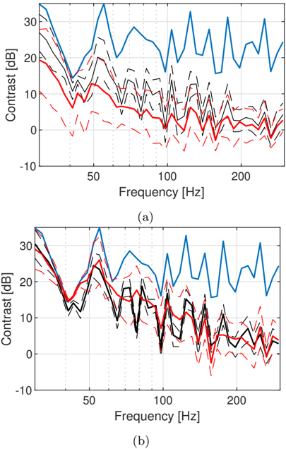It FIG. 8. Contrast results for the dataset with no added uncertainty to the simulated Listening Room (50 different observation masks). (blue): Perfectly known TFs. (black): Deep learning model. (red): Sparse reconstruction. (dashed): ± 1 standard deviation. <details> <summary>Image 8 Details</summary>  ### Visual Description ## Chart: Contrast vs. Frequency ### Overview The image presents two line charts, (a) and (b), each displaying the relationship between "Contrast [dB]" on the y-axis and "Frequency [Hz]" on the x-axis. Each chart contains four data series: a blue line, a red line, a black line, and two black dashed lines. The black line appears to represent the mean, while the dashed lines likely represent the standard deviation or confidence interval around the mean. The red and blue lines represent different conditions or data sets. ### Components/Axes * **Y-axis (Contrast):** Labeled "Contrast [dB]", ranges from -10 to 30 with tick marks at -10, 0, 10, 20, and 30. * **X-axis (Frequency):** Labeled "Frequency [Hz]", ranges from approximately 25 to 250 with tick marks at 50, 100, and 200. * **Data Series:** * Blue Line: Represents one condition or data set. * Red Line: Represents another condition or data set. * Black Line (solid): Represents the mean. * Black Dashed Lines: Represent the standard deviation or confidence interval. * **Subplot Labels:** (a) and (b) are placed below their respective charts. ### Detailed Analysis **Chart (a):** * **Blue Line:** Starts at approximately 32 dB at 25 Hz. It decreases to approximately 17 dB at 40 Hz, then increases sharply with high frequency oscillations, reaching peaks around 35 dB. * **Red Line:** Starts at approximately 20 dB at 25 Hz. It decreases to approximately 2 dB at 180 Hz, then increases slightly to approximately 3 dB at 250 Hz. * **Black Line (Mean):** Starts at approximately 28 dB at 25 Hz. It decreases to approximately 2 dB at 180 Hz, then increases slightly to approximately 3 dB at 250 Hz. * **Black Dashed Lines (Standard Deviation):** The dashed lines are positioned above and below the black mean line, indicating the variability in the data. **Chart (b):** * **Blue Line:** Starts at approximately 30 dB at 25 Hz. It decreases to approximately 15 dB at 40 Hz, then increases sharply with high frequency oscillations, reaching peaks around 35 dB. * **Red Line:** Starts at approximately 27 dB at 25 Hz. It decreases to approximately 12 dB at 40 Hz, then decreases to approximately 2 dB at 180 Hz, then increases slightly to approximately 3 dB at 250 Hz. * **Black Line (Mean):** Starts at approximately 29 dB at 25 Hz. It decreases to approximately 12 dB at 40 Hz, then decreases to approximately 2 dB at 180 Hz, then increases slightly to approximately 3 dB at 250 Hz. * **Black Dashed Lines (Standard Deviation):** The dashed lines are positioned above and below the black mean line, indicating the variability in the data. ### Key Observations * The blue line consistently exhibits higher contrast values, especially at higher frequencies, compared to the red line in both charts. * The red line and the black line (mean) are very similar in both charts. * The dashed lines indicate a wider spread of data at lower frequencies, suggesting greater variability in that region. * The two charts (a) and (b) show similar trends for all data series, but the red line in chart (b) starts at a higher contrast value than in chart (a). ### Interpretation The charts compare the contrast levels at different frequencies for two conditions represented by the blue and red lines. The blue line shows a higher contrast, especially at higher frequencies, suggesting that the condition it represents is more responsive or has a stronger signal at those frequencies. The red line shows a lower contrast, indicating a weaker signal or response. The black line represents the average contrast, and the dashed lines show the variability around that average. The similarity between the red line and the black line suggests that the red line condition is closer to the average. The differences between charts (a) and (b), particularly in the starting point of the red line, suggest that there might be slight variations in the experimental setup or conditions between the two measurements. Overall, the data suggests that the blue line condition is significantly different from the red line condition in terms of contrast response across the frequency spectrum. </details> is observed that the deep learning-based model performs better than the sparse reconstruction below 150 Hz for 5 and 15 microphones. Above 150 Hz, both models struggle to provide sufficiently accurate RTFs to create sound zones. In Fig. 9, the model specialized for the Listening Room with l x + U ( -1 . 0 , 1 . 0) m, is compared to the sparse reconstruction. As expected, the resulting performance is reduced for the model. However, it is observed that there is still a benefit when using 5 microphones. At 15 microphones, on the other hand, the performance is comparable for both methods. These results indicate that sound zones could be created based on sound fields extrapolated from very few microphone positions. However, at this stage it requires models which are specialized to the particular room or a narrow range of rooms. Alternatively, it would be required to increase the number of microphones to improve the accuracy of the estimated RTFs. ## VII. CONCLUSION In this paper, deep learning-based sound field reconstruction is evaluated using a new set of extensive mea- FIG. 9. Contrast results for the simulated Listening Room with l x + U ( -1 . 0 , 1 . 0) m (50 different observation masks). (blue): Perfectly known TFs. (black): Deep learning model. (red): Sparse reconstruction. (dashed): ± 1 standard deviation. <details> <summary>Image 9 Details</summary>  ### Visual Description ## Line Charts: Contrast vs. Frequency ### Overview The image contains two line charts, (a) and (b), each displaying the relationship between "Contrast [dB]" on the y-axis and "Frequency [Hz]" on the x-axis. Each chart contains multiple data series represented by lines of different colors and styles (solid, dashed). The charts appear to compare different conditions or measurements, with the blue line consistently showing the highest contrast across the frequency range. ### Components/Axes * **Y-axis (Contrast):** Labeled "Contrast [dB]". The scale ranges from -10 to 30 dB, with tick marks at -10, 0, 10, 20, and 30 dB. * **X-axis (Frequency):** Labeled "Frequency [Hz]". The scale ranges from approximately 20 to 240 Hz, with tick marks at 50, 100, and 200 Hz. * **Data Series:** Each chart contains a blue solid line, a red solid line, and several black dashed lines and a red dashed line. The exact meaning of each line is not specified in the image, but they likely represent different experimental conditions or statistical variations. * **Chart Labels:** The charts are labeled (a) and (b) below the x-axis. ### Detailed Analysis **Chart (a):** * **Blue Solid Line:** This line represents the highest contrast values. It starts at approximately 20 dB at 20 Hz, increases to approximately 35 dB around 60 Hz, and then fluctuates between 15 dB and 35 dB for the rest of the frequency range. * **Red Solid Line:** This line represents a lower contrast value. It starts at approximately 18 dB at 20 Hz, decreases to approximately 5 dB around 100 Hz, and then remains relatively stable between 0 dB and 5 dB for the rest of the frequency range. * **Black Dashed Lines:** These lines show a range of contrast values between the blue and red solid lines. They generally start around 20 dB at 20 Hz, decrease to between 0 dB and 10 dB around 100 Hz, and then fluctuate between 0 dB and 15 dB for the rest of the frequency range. * **Red Dashed Line:** This line represents the lowest contrast values. It starts at approximately 10 dB at 20 Hz, decreases to approximately -5 dB around 70 Hz, and then fluctuates between -5 dB and 5 dB for the rest of the frequency range. **Chart (b):** * **Blue Solid Line:** Similar to chart (a), this line represents the highest contrast values. It starts at approximately 20 dB at 20 Hz, increases to approximately 35 dB around 60 Hz, and then fluctuates between 15 dB and 35 dB for the rest of the frequency range. * **Red Solid Line:** This line represents a lower contrast value. It starts at approximately 25 dB at 20 Hz, decreases to approximately 10 dB around 100 Hz, and then remains relatively stable between 5 dB and 15 dB for the rest of the frequency range. * **Black Dashed Lines:** These lines show a range of contrast values between the blue and red solid lines. They generally start around 25 dB at 20 Hz, decrease to between 5 dB and 15 dB around 100 Hz, and then fluctuate between 0 dB and 15 dB for the rest of the frequency range. * **Red Dashed Line:** This line represents the lowest contrast values. It starts at approximately 15 dB at 20 Hz, decreases to approximately 0 dB around 70 Hz, and then fluctuates between -5 dB and 10 dB for the rest of the frequency range. ### Key Observations * In both charts, the blue line consistently exhibits the highest contrast across the frequency spectrum. * The red solid line and black dashed lines show a general decreasing trend in contrast as frequency increases, especially up to 100 Hz. * The red dashed line consistently shows the lowest contrast values in both charts. * The contrast values tend to fluctuate more at higher frequencies (above 100 Hz) compared to lower frequencies. * Chart (b) shows a slightly higher contrast for the red solid line and black dashed lines at lower frequencies compared to chart (a). ### Interpretation The charts likely represent the contrast performance of a system or device across different frequencies under different conditions. The blue line could represent an ideal or maximum performance scenario, while the red solid line and black dashed lines represent more typical or varied performance levels. The red dashed line might represent a worst-case scenario or a specific degraded condition. The data suggests that the system's contrast performance is generally better at lower frequencies, with a noticeable drop-off as frequency increases, especially up to 100 Hz. The fluctuations at higher frequencies could indicate increased noise or instability in the system's response. The difference between charts (a) and (b) suggests that there is a slight variation in the system's performance under different conditions, with chart (b) showing a slightly better contrast at lower frequencies for the red solid line and black dashed lines. This could be due to variations in experimental setup, environmental factors, or system parameters. </details> surements from real rooms, which are released alongside the paper. The focus of the work is threefold: examine performance of simulation-based learning of magnitude reconstruction in real rooms, extend reconstruction to complex-valued sound fields, and show a sound zone application taking advantage of the reconstructed sound fields. Experiments for each of the three directions indicate promising aspects of data-driven sound field reconstruction, even with a low number of arbitrarily placed microphones. In the future, it would be of interest to investigate whether transfer learning can help bridge the discrepancies between simulated and real data. With the addition of more rooms, some could be used in the training phase. Furthermore, three-dimensional reconstruction can be achieved using available convolutional models designed specifically to solve three-dimensional problems. ## ACKNOWLEDGMENTS This work is part of the ISOBEL Grand Solutions project, and is supported in part by the Innovation Fund Denmark (IFD) under File No. 9069-00038A. - 1 The data are collected under the Interactive Sound Zones for Better Living (ISOBEL) project, which aims to develop interactive sound zone systems, responding to the need for sound exposure control in dynamic real-world contexts, adapted to and tested in healthcare and homes. The ISOBEL Sound Field dataset can be accessed at https://doi.org/10.5281/zenodo.4501339 . - 2 Further details of the experimental setup and protocol, e.g. equipment, are available in the measurement reports included with the dataset. 3 See footnote 2. 4 Room B has measurements at a single height: 1 meter above the floor. - 5 The use case with multiple individual audio signals can be realized using superposition of this solution and one where the role of bright and dark zone are reversed. - Ajdler, T., Sbaiz, L., and Vetterli, M. ( 2006 ). 'The Plenacoustic Function and Its Sampling,' IEEE Transactions on Signal Processing 54 (10), 3790-3804, doi: 10.1109/TSP.2006.879280 . - Antonello, N., Sena, E. D., Moonen, M., Naylor, P. A., and van Waterschoot, T. ( 2017 ). 'Room Impulse Response Interpolation Using a Sparse Spatio-Temporal Representation of the Sound Field,' IEEE/ACM Transactions on Audio, Speech, and Language Processing 25 (10), 1929-1941, doi: 10.1109/TASLP.2017. 2730284 . - Bertalmio, M., Sapiro, G., Caselles, V., and Ballester, C. ( 2000 ). 'Image inpainting,' in Proceedings of the 27th Annual Conference on Computer Graphics and Interactive Techniques , SIGGRAPH '00, ACM Press/Addison-Wesley Publishing Co., USA, pp. 417-424, doi: 10.1145/344779.344972 . - Betlehem, T., Zhang, W., Poletti, M. A., and Abhayapala, T. D. ( 2015 ). 'Personal Sound Zones: Delivering interface-free audio to multiple listeners,' IEEE Signal Processing Magazine 32 (2), 81-91, doi: 10.1109/MSP.2014.2360707 . - Cecchi, S., Carini, A., and Spors, S. ( 2018 ). 'Room Response Equalization-A Review,' Applied Sciences 8 (1), 16, doi: 10. 3390/app8010016 . - Choi, J., and Kim, Y. ( 2002 ). 'Generation of an acoustically bright zone with an illuminated region using multiple sources,' Journal of the Acoustical Society of America 111 (4), 1695-1700. - Dong, C., Loy, C. C., He, K., and Tang, X. ( 2016 ). 'Image SuperResolution Using Deep Convolutional Networks,' IEEE Transactions on Pattern Analysis and Machine Intelligence 38 (2), 295307, doi: 10.1109/TPAMI.2015.2439281 . - Elliott, S. J., Cheer, J., Choi, J., and Kim, Y. ( 2012 ). 'Robustness and regularization of personal audio systems,' IEEE Transactions on Audio, Speech, and Language Processing 20 (7), 21232133. - Farina, A. ( 2000 ). 'Simultaneous Measurement of Impulse Response and Distortion with a Swept-Sine Technique,' in Proceedings of the Audio Engineering Society Convention 108 . - Fernandez-Grande, E. ( 2019 ). 'Sound field reconstruction in a room from spatially distributed measurements,' in 23rd International Congress on Acoustics , pp. 4961-68. - Genovese, A. F., Gamper, H., Pulkki, V., Raghuvanshi, N., and Tashev, I. J. ( 2019 ). 'Blind Room Volume Estimation from Singlechannel Noisy Speech,' in ICASSP 2019 - 2019 IEEE International Conference on Acoustics, Speech and Signal Processing (ICASSP) , pp. 231-235, doi: 10.1109/ICASSP.2019.8682951 . - Glorot, X., and Bengio, Y. ( 2010 ). 'Understanding the difficulty of training deep feedforward neural networks,' in Proceedings of the Thirteenth International Conference on Artificial Intelligence and Statistics , pp. 249-256. - ISO 3382-2:2008 ( 2008 ). 'Acoustics - Measurement of room acoustic parameters - Part 2: Reverberation time in ordinary rooms,' Standard. - ITU-R BS.1116-3 ( 2015 ). 'Methods for the subjective assessment of small impairments in audio systems,' Standard. - Jacobsen, F., and Juhl, P. M. ( 2013 ). Fundamentals of General Linear Acoustics (John Wiley & Sons). - Karjalainen, M., Makivirta, A., Antsalo, P., and Valimaki, V. ( 2001 ). 'Low-frequency modal equalization of loudspeaker-room responses,' in Audio Engineering Society Convention 111 . - Kim, J., El-Khamy, M., and Lee, J. ( 2020 ). 'T-GSA: Transformer with Gaussian-Weighted Self-Attention for Speech Enhancement,' in ICASSP 2020 - 2020 IEEE International Conference on Acoustics, Speech and Signal Processing (ICASSP) , pp. 6649-6653, doi: 10.1109/ICASSP40776.2020.9053591 . - Kingma, D. P., and Ba, J. ( 2014 ). 'Adam: A Method for Stochastic Optimization,' arXiv:1412.6980 [cs] . - Ledig, C., Theis, L., Huszar, F., Caballero, J., Cunningham, A., Acosta, A., Aitken, A., Tejani, A., Totz, J., Wang, Z., and Shi, W. ( 2017 ). 'Photo-realistic single image super-resolution using a generative adversarial network,' in Proceedings of the IEEE Conference on Computer Vision and Pattern Recognition (CVPR) . - Liu, G., Reda, F. A., Shih, K. J., Wang, T.-C., Tao, A., and Catanzaro, B. ( 2018 ). 'Image Inpainting for Irregular Holes Using Partial Convolutions,' in Computer Vision - ECCV 2018 , edited by V. Ferrari, M. Hebert, C. Sminchisescu, and Y. Weiss, Lecture Notes in Computer Science, Springer International Publishing, Cham, pp. 89-105, doi: 10.1007/978-3-030-01252-6\_6 . - Llu´ ıs, F., Mart´ ınez-Nuevo, P., Møller, M. B., and Shepstone, S. E. ( 2020 ). 'Sound field reconstruction in rooms: Inpainting meets super-resolution,' The Journal of the Acoustical Society of America 148 (2), 649-659, doi: 10.1121/10.0001687 . - Mignot, R., Chardon, G., and Daudet, L. ( 2014 ). 'Low Frequency Interpolation of Room Impulse Responses Using Compressed Sensing,' IEEE/ACM Transactions on Audio, Speech, and Language Processing 22 (1), 205-216, doi: 10.1109/TASLP. 2013.2286922 . - Møller, M. B., and Østergaard, J. ( 2020 ). 'A Moving Horizon Framework for Sound Zones,' IEEE/ACM Transactions on Audio, Speech, and Language Processing 28 , 256-265, doi: 10.1109/TASLP.2019.2951995 . - Nowakowski, T., de Rosny, J., and Daudet, L. ( 2017 ). 'Robust source localization from wavefield separation including prior information,' The Journal of the Acoustical Society of America 141 (4), 2375-2386, doi: 10.1121/1.4979258 . - Radlovic, B. D., Williamson, R. C., and Kennedy, R. A. ( 2000 ). 'Equalization in an acoustic reverberant environment: Robustness results,' IEEE Transactions on Speech and Audio Processing 8 (3), 311-319, doi: 10.1109/89.841213 . - Ronneberger, O., Fischer, P., and Brox, T. ( 2015 ). 'U-Net: Convolutional Networks for Biomedical Image Segmentation,' in Medical Image Computing and Computer-Assisted Intervention - MICCAI 2015 , edited by N. Navab, J. Hornegger, W. M. Wells, and A. F. Frangi, Lecture Notes in Computer Science, Springer International Publishing, Cham, pp. 234-241, doi: 10.1007/978-3-319-24574-4\_28 . - Tylka, J. G., and Choueiri, E. ( 2015 ). 'Comparison of techniques for binaural navigation of higher-order ambisonic soundfields,' in Audio Engineering Society Convention 139 . - Verburg, S. A., and Fernandez-Grande, E. ( 2018 ). 'Reconstruction of the sound field in a room using compressive sensing,' The Journal of the Acoustical Society of America 143 (6), 3770-3779, doi: 10.1121/1.5042247 . - Vu, T. P., and Lissek, H. ( 2020 ). 'Low frequency sound field reconstruction in a non-rectangular room using a small number of microphones,' Acta Acustica 4 (2), 5, doi: 10.1051/aacus/2020006 . - Yang, M., Ma, M. Q., Li, D., Tsai, Y. H., and Salakhutdinov, R. ( 2020 ). 'Complex Transformer: A Framework for Modeling Complex-Valued Sequence,' in ICASSP 2020 - 2020 IEEE International Conference on Acoustics, Speech and Signal Processing (ICASSP) , pp. 4232-4236, doi: 10.1109/ICASSP40776.2020. 9054008 . - Yu, W., and Kleijn, W. B. ( 2021 ). 'Room Acoustical Parameter Estimation From Room Impulse Responses Using Deep Neural Networks,' IEEE/ACM Transactions on Audio, Speech, and Language Processing 29 , 436-447, doi: 10.1109/TASLP.2020. 3043115 .