## A Deep and Wide Neural Network-based Model for Rajasthan Summer Monsoon Rainfall (RSMR) Prediction
Vikas Bajpai ∗ · Anukriti Bansal ∗
Received: date / Accepted: date
Abstract Importance of monsoon rainfall cannot be ignored as it affects round the year activities ranging from agriculture to industrial. Accurate rainfall estimation and prediction is very helpful in decision making in the sectors of water resource management and agriculture. Due to dynamic nature of monsoon rainfall, it's accurate prediction becomes very challenging task. In this paper, we analyze and evaluate various deep learning approaches such as one dimensional Convolutional Neutral Network, Multi-layer Perceptron and Wide Deep Neural Networks for the prediction of summer monsoon rainfall in Indian state of Rajasthan.For our analysis purpose we have used two different types of datasets for our experiments. From IMD grided dataset, rainfall data of 484 coordinates are selected which lies within the geographical boundaries of Rajasthan. We have also collected rainfall data of 158 rain gauge station from water resources department. The comparison of various algorithms on both these data sets is presented in this paper and it is found that Deep Wide Neural Network based model outperforms the other two approaches.
Keywords Deep learning · rainfall prediction · machine learning · wide and deep neural network · multilayer perceptron (MLP) · convolutional neural network (CNN) · Summer Monsoon Rainfall
∗ The authors contributed equally
V. Bajpai The LNM Institute of Information Technology Jaipur, Rajasthan, India
E-mail: vikas.bajpai87@gmail.com
A. Bansal
The LNM Institute of Information Technology
Jaipur, Rajasthan, India
E-mail: anukriti1107@gmail.com
## 1 Introduction
Understanding of rainfall characteristics is important for a variety of activities including efficient engineering, planning and management of water resources [27, 7]. In addition to this, rainfall play a major role in balancing of various activities such as, hydrologic cycle, water availability for terrestrial animals, agriculture and industrial processes. Rainfall and its estimation is not only important for India but is equally important for the entire globe [31, 72, 12, 19, 2, 35, 28, 40].
In India majority of the rain is received from the month of June to September (June-July-August-September) and that is why this period is called as Indian Summer Monsoon Rainfall (ISMR) or the Southwest monsoon rainfall. Cultivated land in India is majorly benefited by this ISMR [71] which makes this season highly important and ultimately prediction and estimation of rainfall for this period also becomes equally essential. India receives nearly 80 percent rainfall during summer monsoon period [46, 48, 45] only. This summer monsoon rainfall fuhrer helps in predicting food grain production [53] which ultimately contributes to country's GDP ∗ . Prediction and estimation of ISMR started way back from the year 1903 as people started believing on the importance of this monsoon rainfall [75].
In this work, our area of study is Rajasthan which is the largest state of India and the 60% of its area falls under the arid category which makes it very environmentally sensitive [17]. Even after being an arid to semi-arid zone, Rajasthan has observed several floods in the past [24, 77, 57]and also observed several droughts [34, 5, 23, 47, 52]. An early indication of the amount of monsoon rainfall a particular region is going to receive, can be very handy in terms of managing the water resource for the entire year. This early indication can give us an idea about the amount of availability of water in a particular reservoir. Now this reservoir which will cater to the needs of demand from people and industry in a particular area can be regulated and measures can be taken well in advance for proper water resource management for the monsoon and non-monsoon period.
There are several indicators on which rainfall depends, such as surface temperature, sea level, distance from sea, distance from mountain ranges etc. In this work, we propose a time series based approach for the prediction of rainfall for the months of June, July, August and September (summer monsoon months). For this we collected Indian Meteorological Department ( IMD hereafter) grided data of 118 years ( from the year 1901 to 2018) and station data of 61 years( from the year 1957 to 2017) from Water Resources Department, Rajasthan (WRD hereafter). In this work we design and analyze advance deep learning models to capture the patterns from this historical time series data for the prediction of Rajasthan summer monsoon rainfall (RSMR hereafter). For this we adapt and improve a model originally proposed by Cheng et al [10] in the field of recommender systems. We name our proposed model as Deep
∗ https://statisticstimes.com/economy/country/india-gdp-growth-sectorwise.php
and Wide Monsoon Rainfall Prediction Model (DWMRPM hereafter) and compared with advance deep-learning based models like multi-layer perceptron (MLP), one dimensional convolutional neural network (1D-CNN) based neural networks
## 1.1 Related Work
In past researchers have applied numerical[15] and statistical models[41, 44] for rainfall prediction. But with gaining popularity of artificial intelligence and increasing machine computation power, training abundant data using machine learning and deep learning models are becoming the center of attraction for researchers [78]. One of the major reasons of scientists switching from traditional numerical approaches to artificial intelligence based approaches is that the statistical and numerical models fail to capture the dynamic nature of rainfall [65] whereas neural networks are quiet smart in capturing the hidden trends and seasonality existing in time series rainfall data. The numerical and statistical models were used majorly for two to three decades but these methods lacked forecasting accuracy [21] resulting into failure in predicting major rainfall variations [33, 64]. There are evidences from the past where these numerical methods failed [20, 55] to predict the monsoon rainfall and severe droughts were observed.
Pritpal [68] has made an attempt to predict the ISMR using monthly monsoon rainfall values and applied fuzzy sets and artificial neural network (ANN). When the parameters on which the rainfall depends are very high then in order to predict ISMR, [60] used auto encoder [49] for reducing the number of parameter and then predicted the ISMR. [61] studied the climatic variables responsible for ISMR and used deep learning feature for monsoon rainfall prediction.This study also shows the monsoon deviation from long period average (LPA) rainfall. Johny et al used an adaptive Ensemble Model of ANN which was capable of capturing very low and very high rainfall in the Indian state of Kerala [32]. Dubey et. al [14] used three artificial neural network based algorithms ( feed-forward back propagation algorithm, layer recurrent algorithm and feed-forward distributed time delay algorithm) for rainfall prediction over the region of Pondicherry, India. Some amount of monsoon rainfall prediction is done by applying feed forward neural network [8, 62, 70].
Fluctuations in the summer monsoon rainfalls can't be captured efficiently by traditional linear statistical models [69, 13]. This motivated us to use Deep Learning based model which are efficient in capturing this non-linearity and dynamic nature of ISMR. As per IMD weather forecasting manual † , Indian rainfall is very well known for its variability in space and time. There is hardly any seasonal distribution of rainfall over entire India. At two different station locations which are a few miles apart, if we consider one day rainfall, we may observe that one station experiencing heavy rainfall whereas the other
† https://imdpune.gov.in/Weather/Forecasting Mannuals/IMD IV-13.pdf
station may go completely dry. This kind of variation is not only found in monsoon rainfall period(June to September) but also during post monsoon period (October to December) as well.
A good amount amount of work has been done in the field of ISMR as presented above but at present to the best of our knowledge, no work is done in the field of RSMR prediction, which attracted the authors of this paper to explore this untouched area. An attempt to predict the agricultural drought index in Rajasthan is done by Dutta et al [16] using standardized precipitation index. In this proposed work, an extensive study is done in predicting RSMR for the first time. The good thing about Rajasthan is the strong Rain Gauge network from IMD, Water Resource Department, Rajasthan and the Revenue Department which has resulted into the abundant supply of rainfall data for analysis and prediction.
Research work done in the field of Rainfall Prediction and Estimation for the state of Rajasthan is very less. Vikas et al [3] used the historical time-series data for daily rainfall prediction. However worked in analyzing the trends of rainfall in the state of Rajasthan[54, 76]. [6] made an effort to present the holocene variations of monsoon rainfall in Rajasthan. [42] made an attempt to explore the spatial and temporal differences to identify trends in monthly, seasonal and annual rainfall over the Rajasthan region. They observed the prevailing homogeneity of rainfall at various stations in the state. In another work [66] authors tried to estimate the one day maximum rainfall in Jhalrapatan, a city in the state of Rajasthan. Authors have done the probability analysis for this purpose. [39] studied the rainfall pattern in Chaksu, Rajasthan.
Our objective is to predict the RSMR which starts in the month of June and ends in the month of September. In this work we propose a time series based prediction model which depends on the fundamental of present and future time series data dependency on past time series data [67]. We adapt and improvise wide and deep learning model originally proposed by Cheng et al [10] for recommendations. Many authors h ave used this concept in different domains like regression analysis [36], quality prediction [58], rainfall prediction [3] etc. Wide networks are used for memorization and deep networks are used for generalization. In this work we propose a Deep and Wide Monsoon Rainfall Prediction Model (hereafter DWMRPM) to predict monsoon rainfall prediction in the Indian state of Rajasthan.
The rest of the paper is organized as follows. Section 2 explains the proposed model for summer monsoon rainfall in Rajasthan. Details of experimental evaluations, model training, results of rainfall prediction and comparison with other deep learning approaches is given in section 3. Finally we conclude the paper in Section 4 and provide avenues for future work.
## 1.2 Major Contributions
1. In this work, we propose a novel architecture based on deep and wide neural network for the purpose of summer monsoon rainfall using historical time-
- series data. The model efficiently captures the dynamic nature of monsoon rainfall and works well in its prediction. To the best of our knowledge, we are the first who have tried to solve this challenging problem.
2. We compare our work with various advanced deep learning algorithms for sequence prediction on two different types of datasets and have obtained very promising results.
3. The algorithms we designed has the generalization ability and can be used to predict summer monsoon rainfall for atmospherically different regions of Rajasthan.
## 2 Deep & Wide Monsoon Rainfall Prediction Model (DWMRPM)
This section first provides a brief overview of the proposed approach and subsequently explain various steps involved in the prediction of Rajasthan summer monsoon rainfall (RSMR, hereafter).
## 2.1 Overview
In this work we address the problem of summer monsoon rainfall in Rajasthan, which is the largest state of India and is located in the North-Western part of the country. Rajasthan has very distinct physiographic characteristics. On one side it has India's biggest desert area, called The Thar Dessert and on the other side this state has Eastern Plains and the ranges of Aravalli Hills [18]. These ranges are in the direction of South-west monsoon, which is responsible for rainfall in the region [59]. Atmospherically Rajasthan is divided into four zones: North West Desert Region, Central Aravalli Hill Region, Eastern Plains and South Eastern Plateau Region [73]. Details of the districts, which come under the respective zones are given below:
North-West Desert Region: Jaisalmer, Jodhpur, Hanumangarh, Shriganganagar, Barmer, Churu, Nagaur, Pali, Sikar, Bikaner and Jhunjhunu Central Aravalli Hill Region: Udaipur, Dungarpur, Sirohi, Jalore, Pali, Banswara, Bhilwara, Chittorgarh, Rajsamand and Ajmer
Eastern Plains: Alwar, Bharatpur, Tonk, Sawai Madhopur, Karauli, Jaipur, Dausa and Dhoulpur
South-Eastern Plateau Region: Kota, Bundi, Jhalawar and Baran
All these zones have different atmospheric and climatic conditions. The problem of predicting summer monsoon rainfall in Rajasthan is different from the prediction of Indian summer monsoon rainfall (ISMR, hereafter). Most of the time-series-based methods for predicting ISMR consider average monthly rainfall values by taking weighted average of the 306 well distributed raingauge stations in the non-hilly areas of Indian sub-continent [13, 69, 70, 62]. Rajasthan being a dry state lies in arid and semi-arid zones and characterized by low and uneven rainfall [38], therefore, a dedicated system is required which
can predict monsoon rainfall for different geographical regions separately. We use historical monthly rainfall data from two different sources to train and analyze the performance of our model in prediction of Rajasthan Summer Monsoon Rainfall. Details on the datasets are given in Section 2.2
For ISMR researchers used monthly rainfall values of June to September across all the years [13] or just have captured the dependency of months of a single year [68] In order to avoid loss of any information, we are using rainfall values of all the months of previous years for the prediction of rainfall for the months of June, July, August and September. For example in order to predict rainfall for the month of June 2019, we use rainfall values of all the months from May 2000 to May 2019.
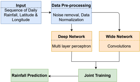
In this work, we propose a deep and wide monsoon rainfall prediction model (DWMRPM) for the prediction of the total monthly rainfall intensity for the summer monsoons months of Rajasthan. The wide network is used to extract low-dimensional features. Here, instead of using a sequence of monthly rainfall values directly, we are using features obtained after applying a convolutional layer, as it is very effective in learning spatial dependencies in and between the series of data [74]. High-dimensional features, on the other hand, are derived using Multi-layer perceptron (MLP) [51] in which a sequence of rainfall intensity values are passed on to a deep network. In order to incorporate a geographical generalization ability in the model, so that a single model can be used to make rainfall predictions in different geographical conditions, information of geographical parameters (latitude and longitude) is included at the time of training. The operational steps involved in the development of our proposed DWMRPM for the prediction of rainfall are shown in Figure 1.
Fig. 1: Overview of DWMRPM: The model takes sequence of monthly rainfall intensities and geographical parameters, namely latitude and longitude as input. After initial pre-processing, input is fed to a deep network, which is a multi-layer perceptron, and to a wide network, which is a convolutional network. The model is jointly trained considering the activation weights from both deep and wide networks simultaneously.
<details>
<summary>Image 1 Details</summary>
### Visual Description
## Diagram: Rainfall Prediction Model
### Overview
The image is a flowchart illustrating a rainfall prediction model. It outlines the steps from input data to the final rainfall prediction, incorporating data pre-processing, deep and wide networks, and joint training.
### Components/Axes
The diagram consists of several rectangular blocks representing different stages of the model. The blocks are connected by arrows indicating the flow of data. The blocks are colored in blue, orange, and green.
* **Input (Top-Left, Blue):** "Input" and "Sequence of Daily Rainfall, Latitude & Longitude"
* **Data Pre-processing (Top-Center, Blue):** "Data Pre-processing" and "Noise removal, Data Normalization"
* **Deep Network (Center-Left, Orange):** "Deep Network" and "Multi layer perceptron"
* **Wide Network (Center-Right, Orange):** "Wide Network" and "Convolutions"
* **Joint Training (Bottom-Center, Green):** "Joint Training"
* **Rainfall Prediction (Bottom-Left, Green):** "Rainfall Prediction"
### Detailed Analysis or Content Details
1. **Input:** The process begins with input data, which includes a sequence of daily rainfall, latitude, and longitude.
2. **Data Pre-processing:** The input data is then pre-processed. This involves noise removal and data normalization.
3. **Deep Network:** One branch of the model utilizes a deep network, specifically a multi-layer perceptron.
4. **Wide Network:** Another branch employs a wide network using convolutions.
5. **Joint Training:** The outputs from both the deep and wide networks are combined in a joint training stage.
6. **Rainfall Prediction:** Finally, the model produces a rainfall prediction based on the joint training.
The flow of data is as follows:
* Input -> Data Pre-processing
* Data Pre-processing -> Deep Network
* Data Pre-processing -> Wide Network
* Deep Network -> Joint Training
* Wide Network -> Joint Training
* Joint Training -> Rainfall Prediction
* Rainfall Prediction -> Joint Training (Feedback Loop)
### Key Observations
* The model uses both deep and wide networks, suggesting a hybrid approach to capture different aspects of the data.
* The joint training stage indicates that the outputs of the two networks are combined to improve prediction accuracy.
* There is a feedback loop from Rainfall Prediction to Joint Training.
### Interpretation
The diagram illustrates a machine learning model designed for rainfall prediction. The model leverages both deep learning (multi-layer perceptron) and wide learning (convolutions) techniques. The pre-processing step is crucial for cleaning and normalizing the input data, ensuring the model receives high-quality information. The joint training phase likely aims to integrate the strengths of both network types, potentially improving the overall accuracy and robustness of the rainfall prediction. The feedback loop from Rainfall Prediction to Joint Training suggests that the model is continuously learning and refining its predictions based on past results.
</details>
To evaluate the performance of the proposed method, we use two standard statistical metrics, namely mean absolute error (MAE) and root mean square error (RMSE). We compare our results with the advance deep learning models like MLP and one dimensional convolutional neural networks (1-DCNN) which are very popular for sequence based predictions.
## 2.2 Dataset description and pre-processing
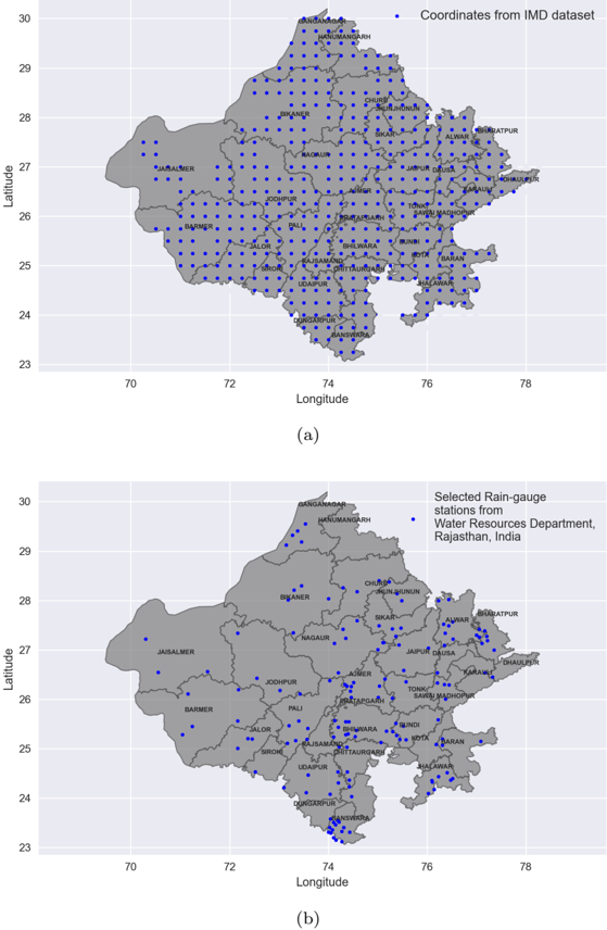
In this work we have used Water Resources Department dataset and Indian Meteorological Department (IMD) gridded rainfall data with a high spatial resolution of 0 . 25 ◦ × 0 . 25 ◦ [50]. From IMD data set, we selected the rainfall data of the Rajasthan meteorological sub-division ranging from 23 ◦ 3 . 5 ′ Nto 30 ◦ 14 ′ N latitude and 69 ◦ 27 ′ E to 78 ◦ 19 ′ E longitude, for the period of 118 years from the year 1901 to 2018. It gave the rainfall data for 1008 rain-gauge stations. We have also collected the rainfall data from Rajasthan's water resources department, for more than 500 rain-gauge stations, over a period of 61 years (from the year 1957 to 2017). The datasets were noisy in terms of negative and missing values. After initial level data pre-processing and cleansing steps, we selected 484 co-ordinates from IMD dataset of High Spatial Resolution of (0.25X0.25 degree) and 158 stations from Rajasthan's water resources data for our analysis. The distribution of the selected stations from water resources data, over 33 districts are depicted on the map of Rajasthan in Figure 2
In this paper, authors have made use of both the Station data (data collected from various Rain Gauge Stations in Rajasthan) and the Gridded data [50]. The idea behind using both the data sets is that when only the station data is used, for experimentation, one uses the data for single point of scale whereas when the gridded data is used the application of different meteorological data for a region is applied depending upon the resolution. In large catchment areas where less number of Rain Gauges are installed, modeling may not be that much accurate, on the other hand gridded data is more continuous and may prove better than single point estimates. Gridded data contains the data from stations or satellites (in our case, it's rain gauge station data) which undergoes interpolation over a grid. This interpolation needs careful analysis for biases and outliers [56, 50]. Station data on the other hand is unbiased single point data. For our study, we have used quality controlled data sets from both the categories. If someone has enough single point station in the region under study, then the station data can be easily utilized but since the rain gauge distribution is not uniform ( as shown in Raj WRD), specially in the dessert areas where the rain gauge station installation density is very low, combination of both the data set seems to be optimal. Another advantage of using gridded data is that it acts as a source of replacement to the data missing from the records of rain gauge stations[43]. Any area or zone where the observed station data (point data) is comparatively less, interpolated gridded data can work as a potential alternative means [4].
Fig. 2: Map of Rajasthan showing distribution of (a) selected 484 coordinates from IMD gridded dataset at high spatial resolution of . 25 ◦ × . 25 ◦ , (b) selected 158 rain-gauge stations from Water Resources Department, Rajasthan. The rainfall data obtained from these coordinates and rain-gauge stations are used for the prediction of Rajasthan summer monsoon rainfall (RSMR)
<details>
<summary>Image 2 Details</summary>
### Visual Description
## Map: Rajasthan Rain Gauge Locations
### Overview
The image presents two maps of Rajasthan, India, showing the locations of rain gauges. Map (a) displays coordinates from the IMD (India Meteorological Department) dataset, while map (b) shows selected rain-gauge stations from the Water Resources Department, Rajasthan. Both maps depict the state's outline, major cities, and the distribution of rain gauge locations as blue dots.
### Components/Axes
* **Map Outline:** The grey outline represents the state of Rajasthan, India.
* **Latitude Axis (Y-axis):** Ranges from approximately 23 to 30.
* **Longitude Axis (X-axis):** Ranges from approximately 70 to 78.
* **City Labels:** Names of cities are overlaid on the map.
* **Blue Dots:** Represent rain gauge locations.
* **Legends:**
* **(a):** "Coordinates from IMD dataset" (top-right)
* **(b):** "Selected Rain-gauge stations from Water Resources Department, Rajasthan, India" (top-right)
### Detailed Analysis
**Map (a): Coordinates from IMD dataset**
* The blue dots are distributed relatively evenly across the state, forming a grid-like pattern.
* The density of points appears higher in the eastern part of the state.
* The coordinates are spaced approximately 0.25 degrees apart in both latitude and longitude.
**Map (b): Selected Rain-gauge stations from Water Resources Department, Rajasthan, India**
* The blue dots are distributed unevenly, with clusters in certain regions and sparse coverage in others.
* There is a higher concentration of rain gauges in the southeastern and eastern parts of the state.
* The western part of the state has fewer rain gauges.
* The rain gauges appear to be located near cities and towns.
**City Locations (Both Maps):**
* Major cities labeled include: Ganganagar, Hanumangarh, Churu, Jhunjhunun, Bikaner, Sikar, Nagaur, Alwar, Bharatpur, Jaisalmer, Jaipur, Dausa, Dhaulpur, Jodhpur, Ajmer, Karauli, Barmer, Pali, Tonk, Sawai Madhopur, Bundi, Jalore, Sirohi, Bhilwara, Kota, Baran, Jhalawar, Udaipur, Chittaurgarh, Dungarpur, Banswara.
### Key Observations
* Map (a) provides a systematic grid of coordinates, likely for comprehensive data collection.
* Map (b) shows the actual locations of rain gauges managed by the Water Resources Department, which are not uniformly distributed.
* The eastern and southeastern regions of Rajasthan have a higher density of rain gauges in map (b) compared to the western region.
### Interpretation
The two maps provide different perspectives on rain gauge locations in Rajasthan. Map (a) represents a theoretical or planned distribution of data collection points, while map (b) shows the actual distribution of operational rain gauges. The difference in distribution suggests that the Water Resources Department may prioritize certain regions for monitoring, possibly due to higher rainfall, agricultural importance, or water resource management needs. The IMD dataset likely serves a broader purpose of weather monitoring and forecasting, hence the systematic grid. The clustering of rain gauges in the southeastern part of the state could indicate a region with higher rainfall variability or greater water resource demands.
</details>
These datasets contained daily rainfall values from which we calculated monthly rainfall values for January to December. In order to provide rainfall
pattern in Rajasthan, mean rainfall values for each month and the monsoon season (combined rainfall of June, July, August and September) from the year 1901-2018 for a randomly picked rain-gauge station is shown in Table 1. We also provide the minimum and maximum rainfall for each month and monsoon season, over the duration of 118 years. It can be observed that the significant amount of annual rainfall occurs in the monsoon months and the in the remaining months, the aggregate rainfall is very less.
Table 1: Statistical summary of monthly data for the IMD dataset and the dataset from the water resource department of Rajasthan (WRD). Mean, maximum and minimum rainfall fall values of IMD are shown for a randomly picked coordinate at 26 ◦ 0 ′ N and 74 ◦ 5 ′ E for a period of 118 years from 1901 to 2018. The rainfall statistics for WRD dataset for a randomly picked rain-gauge station, situated at 26 ◦ 04 ′ N and 75 ◦ 01 ′ E is shown for a period of 61 years from the year 1957 to 2017.
| Month | Mean (mm) | Mean (mm) | Maximum (mm) | Maximum (mm) | Minimum (mm) | Minimum (mm) |
|------------------|-------------|-------------|----------------|----------------|----------------|----------------|
| Month | IMD | WRD | IMD | WRD | IMD | WRD |
| Jan | 4.24 | 2.20 | 63.66 | 53.00 | 0 | 0 |
| Feb | 4.22 | 2.40 | 65.56 | 54.00 | 0 | 0 |
| Mar | 3.81 | 2.11 | 64.44 | 74.00 | 0 | 0 |
| Apr | 2.91 | 3.78 | 43.03 | 56.00 | 0 | 0 |
| May | 9.14 | 5.72 | 90.75 | 87.00 | 0 | 0 |
| Jun | 49.67 | 41.92 | 246.2 | 227.00 | 0 | 0 |
| Jul | 159.45 | 150.54 | 523.5 | 476.00 | 13.11 | 10 |
| Aug | 160.86 | 166.05 | 441 | 905.0 | 3.41 | 40.8 |
| Sep | 65.38 | 63.83 | 305.8 | 402.00 | 0 | 0 |
| Oct | 9.84 | 7.31 | 154.4 | 132.00 | 0 | 0 |
| Nov | 1.72 | 4.02 | 25.67 | 160.00 | 0 | 0 |
| Dec | 2.31 | 1.04 | 46.53 | 30.00 | 0 | 0 |
| Overall Accuracy | 868.63 | 460.05 | 1080.90 | 937.0 | 91.17 | 102.1 |
We have considered time-series values of monthly rainfall and geographical parameters like latitude and longitude for the prediction of rainfall during the monsoon months in different regions of Rajasthan. The rainfall intensity values ranges from 0 mm to more than 800 mm while coordinate values of latitude and longitude lies between 23 ◦ 3 . 5 ′ N to 30 ◦ 14 ′ N and 69 ◦ 27 ′ to 78 ◦ 19 ′ E, respectively. Since the data is of different dimensions and dimensional units, therefore we normalize the data to make it dimensionally uniform. When the magnitude of different parameters in a dataset is different, the parameters with higher values suppresses the role of the parameters with lower values in model training. To handle this issue, we use the min-max normalization method to convert all rainfall intensity values to number between 0 and 100 (latitude and longitude values are already in this range). The mathematical representation of the min-max normalization method is as follows:
<!-- formula-not-decoded -->
where, I ∗ is the normalized value of the monthly rainfall intensity value, I represents a value in the original dataset, I max and I min are the maximum and minimum intensity values, respectively. Normalization can also help in improving the learning capability of the model and in reducing the computational complexity [63].
## 2.3 Model Description
We use deep and wide neural network-based architecture [3] for the purpose of summer monsoon rainfall prediction in the Indian state of Rajasthan. The following paragraphs explains the major components of the model.
## 2.3.1 The Wide Component: Convolutions
The wide component is used to memorize certain combinations of monthly rainfall events, which is beyond the capabilities of the deep model. It is a generalized linear model of type y = w T x + b . In the model proposed by Cheng et al [9], cross-product feature transformations were used as the wide component. In this work we use convolutional network as wide component. The basic components of a general CNN consists of 2 types of layers, namely convolutional layer and pooling layer [25]. The convolutional layer is composed of several convolutional kernels, which capture and learn the correlation of spatial features by computing different feature maps. The output of one dimensional convolutional layer with input size N l is:
<!-- formula-not-decoded -->
where, l is the layer number, w l i,k is the kernel from the i th neuron at layer l -1 to the k th neuron at layer l , a ( l ) , b ( l ) activations, bias at l th layer.
Convolutional layer is followed by a pooling layer that is used to realize shift invariance by reducing the resolution of the feature maps. As demonstrated by [74], 1D CNN performs well in regression type of problems and can learn to find the correlation in between the series very efficiently. Therefore, instead of using raw features in the wide part of the network, we use a convolutional layer to capture such combinations. In addition to this, to make our model more generalized with respect to different atmospheric conditions, we are using geographical parameters namely, longitude and latitude while designing and developing our model (Figure 3).
## 2.3.2 The Deep Component: Multi-layer Perceptron
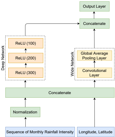
The deep component is a feed-forward neural network, specifically a multilayer perceptron, as shown in Figure 3. Sequence of monthly rainfall intensity
Fig. 3: Selected architecture of DWMRPM for prediction of Rajasthan Summer Monsoon Rainfall. There are two major components: 1.The Deep component consists of mainly an input layer and 3 ReLU layers. 2. The wide component consists of a convolutional layer followed by a global average pooling layer.A sequence of monthly rainfall intensity values after normalization and values are fed to deep and wide components separately
<details>
<summary>Image 3 Details</summary>
### Visual Description
## Diagram: Deep and Wide Neural Network Architecture
### Overview
The image presents a diagram of a deep and wide neural network architecture designed for processing rainfall intensity data along with location coordinates. The network combines a deep branch with multiple ReLU layers and a wide branch with a convolutional layer and a global average pooling layer. The outputs of these branches are concatenated before feeding into the final output layer.
### Components/Axes
* **Input Layers (Blue):**
* Sequence of Monthly Rainfall Intensity
* Longitude, Latitude
* **Green Blocks:** Represent concatenation and normalization operations.
* Normalization
* Concatenate (x2)
* Output Layer
* **Deep Network (Left):** A series of ReLU layers.
* ReLU (300)
* ReLU (200)
* ReLU (100)
* **Wide Network (Right):** A convolutional layer followed by a global average pooling layer.
* Convolutional Layer
* Global Average Pooling Layer
* **Arrows:** Indicate the flow of data through the network.
### Detailed Analysis
1. **Input:** The network takes two inputs: a sequence of monthly rainfall intensity and the longitude/latitude coordinates.
2. **Normalization:** The rainfall intensity sequence is first normalized.
3. **Concatenation (Initial):** The normalized rainfall intensity is concatenated with the longitude/latitude data.
4. **Deep Network:** The concatenated data is fed into a deep network consisting of three ReLU layers with 300, 200, and 100 units, respectively.
5. **Wide Network:** The concatenated data is also fed into a wide network consisting of a convolutional layer followed by a global average pooling layer.
6. **Concatenation (Final):** The outputs of the deep and wide networks are concatenated.
7. **Output Layer:** The concatenated output is fed into the final output layer.
### Key Observations
* The architecture combines a deep network to capture complex temporal patterns in rainfall intensity with a wide network to incorporate spatial information from the location coordinates.
* The use of ReLU activation functions in the deep network helps to mitigate the vanishing gradient problem.
* The global average pooling layer in the wide network reduces the spatial dimensions of the convolutional layer output, making the network more robust to variations in input size.
### Interpretation
This deep and wide neural network architecture is designed to leverage both temporal and spatial information for rainfall prediction or analysis. The deep network is likely intended to learn complex patterns in the rainfall time series, while the wide network incorporates location-specific features. The concatenation of the outputs allows the model to integrate both types of information for improved performance. The architecture is suitable for tasks such as rainfall forecasting, drought monitoring, or flood risk assessment.
</details>
values are given as input, which are then fed into hidden layers of a neural network in the forward pass. Typically, each hidden layer computes:
<!-- formula-not-decoded -->
where, l is the layer number and f is the activation function, rectified linear units (ReLUs) in our case, a ( l ) , b ( l ) , and w ( l ) are the activations, bias and model weights at l th layer.
## 2.3.3 Joint training of the model
The model is trained using the joint training approach that optimizes all parameters simultaneously by taking into account the output of the deep and wide components and their weighted sum. It helps in providing an overall prediction, which is based on aforementioned components, also depicted in Figure 3.
<!-- formula-not-decoded -->
where, y DWMRPM is the prediction, h cn , h d are the output vectors of two sub-models namely wide-convolutional model and deep model respectively, and k cn , k d are their respective weight vectors to be trained.
## 3 Experimental evaluations
## 3.1 Implementation details
All the experimental programs are coded using Keras [11] API of TensorFlow framework [1, 26]. The hardware setup includes computer processor from Intel with i7-8750H configuration supported by 32GB RAM. The upcoming sections and subsections describe the designing and implementation setup of proposed approach and baseline approaches followed by results obtained.
For prediction of monthly rainfall of monsoon season, we consider different training windows of lengths ranging from 2 years to 10 years. We found that 9 years training window gives most accurate prediction results for the monsoon months of June, July August and September.
## 3.1.1 Training, validation and test sets
We use two type of datasets, one from the Indian Meteorological Department (IMD) and the other from the Water Resource Department (WRD). In case of WRD, monthly rainfall values from the year 1957 to 1986 are considered for the purpose of training. Validation of the model is done on the dataset considering the years starting from 1987 to 1997 and finally we test the model on the dataset containing monthly rainfall values in the interval of the year 1998 to 2017. In case of IMD dataset, training is done by considering values from the year 1901 to 1980 and validation is done from the year 1981 to 1995 and finally testing is done on the rainfall intensity values from the year 1996 to 2018.
## 3.1.2 Evaluation metrics
As shown by [22] and [29], to evaluate the overall accuracy of predictions, we use root mean square error (RMSE) and mean absolute error (MAE) as the basic evaluation metrics. Low value of RMSE and MAE means better prediction accuracy of the model.
<!-- formula-not-decoded -->
<!-- formula-not-decoded -->
where, N represents the number of samples, y i is the actual rainfall of the ith sample and y i is the corresponding prediction.
## 3.1.3 Model Training
We optimize various hyper parameters like the batch size, number of hidden layers, number of neuron and the dropout rates using trial-and-error method. The network configuration of DWMRPM used in our experiments is shown in Figure 3. The input to the model is the normalized sequence of monthly rainfall intensity values and actual coordinate values (latitude and longitude). The deep part is a Multi-layer perceptron with an input layer; 3 hidden layers containing 300, 200 and 100 neural units with ReLU as the activation function; and finally a dense output layer.In order to prevent over-fitting of the model, dropout layers [ ? ] with dropout rate 0.3 are added after each hidden layer. The wide part contains a convolutional layer with 100 filters, each of size 1 x 5, followed by a global average pooling layer. The outputs of both the wide and deep networks are concatenated and the model is trained using the joint-training approach, as explained in Section 2.3.3. We use Adam optimizer [37] for training with Mean Square Error (MSE) as loss function, which is calculated as follows:
<!-- formula-not-decoded -->
Here, N represents the number of samples, y i is the actual rainfall of the ith sample and y i is the corresponding prediction. The goal of the model is to find optimized parameters that minimizes MSE
<!-- formula-not-decoded -->
where, θ is the total number of trainable parameters. Weights of the network are initialized using He initialization[30]. Model is trained for 200 epochs with batch size equals to 8.
## 3.1.4 Baseline approaches
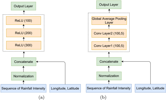
In order to establish the competence of our proposed approach, we have compared the results obtained from the proposed DWMRPM with the results of two advance deep learning approaches: MLP and 1-DCNN. These approaches are working well but not at par with our proposed approach. We have used the same sets of both the data sets for all the approaches in order to avoid any discrepancies that may arise by using different set of datasets for training and testing the models. The network architecture of the baseline approaches, which is selected (after experimenting with various hyper-parameters) for the comparative analysis with the proposed method is explained in the subsequent paragraphs. In all these approaches, we use Adam optimizer for training and MSE as loss function. Input sequence length is 108 (9 years). (Details in Figure 4)
Fig. 4: Architecture of the baseline approaches, selected after experimentation with various hyper-parameters. (a) Network configuration of multi-layer perceptron, and (b) Network configuration of CNN.
<details>
<summary>Image 4 Details</summary>
### Visual Description
## Diagram: Neural Network Architectures for Rainfall Prediction
### Overview
The image presents two distinct neural network architectures, labeled (a) and (b), designed for rainfall prediction. Both architectures take "Sequence of Rainfall Intensity" and "Longitude, Latitude" as inputs. They differ in their internal layer configurations, particularly in how they process the concatenated input data before producing the final output.
### Components/Axes
**General Components (Shared by both architectures):**
* **Input Layers:** "Sequence of Rainfall Intensity" and "Longitude, Latitude" (both in blue boxes).
* **Normalization Layer:** A green box labeled "Normalization".
* **Concatenate Layer:** A green box labeled "Concatenate".
* **Output Layer:** A green box labeled "Output Layer".
* **Arrows:** Indicate the flow of data through the network.
**Architecture (a) Specific Components:**
* **ReLU Layers:** Three orange boxes labeled "ReLU (300)", "ReLU (200)", and "ReLU (100)" stacked vertically within a dashed-line box.
**Architecture (b) Specific Components:**
* **Convolutional Layers:** Two orange boxes labeled "Conv Layer1 (100,5)" and "Conv Layer2 (100,5)" stacked vertically within a dashed-line box.
* **Global Average Pooling Layer:** An orange box labeled "Global Average Pooling Layer".
### Detailed Analysis
**Architecture (a):**
1. **Input:** "Sequence of Rainfall Intensity" and "Longitude, Latitude" are fed into the network.
2. **Normalization:** The inputs are normalized.
3. **Concatenation:** The normalized inputs are concatenated.
4. **ReLU Layers:** The concatenated data passes through three ReLU (Rectified Linear Unit) layers with 300, 200, and 100 units respectively.
5. **Output:** The final output is generated by the "Output Layer".
**Architecture (b):**
1. **Input:** "Sequence of Rainfall Intensity" and "Longitude, Latitude" are fed into the network.
2. **Normalization:** The inputs are normalized.
3. **Concatenation:** The normalized inputs are concatenated.
4. **Convolutional Layers:** The concatenated data passes through two convolutional layers, "Conv Layer1 (100,5)" and "Conv Layer2 (100,5)". The numbers (100,5) likely represent the number of filters and the kernel size, respectively.
5. **Global Average Pooling:** The output of the convolutional layers is fed into a "Global Average Pooling Layer".
6. **Output:** The final output is generated by the "Output Layer".
**Data Flow:**
* In both architectures, the "Longitude, Latitude" input bypasses the Normalization layer and is directly fed into the Concatenate layer.
* The arrows indicate a clear feedforward flow of data from the inputs to the output layer.
### Key Observations
* Both architectures share the same input and output structure, suggesting they are designed to solve the same rainfall prediction task.
* The primary difference lies in the internal processing of the concatenated input data. Architecture (a) uses a stack of ReLU layers, while architecture (b) employs convolutional layers followed by global average pooling.
* The numbers in parentheses after the layer names (e.g., ReLU (100), Conv Layer1 (100,5)) likely represent the number of units or filters and kernel size in each layer, respectively.
### Interpretation
The two architectures represent different approaches to feature extraction and processing for rainfall prediction. Architecture (a) uses fully connected ReLU layers, which can capture complex relationships between the input features but may be prone to overfitting. Architecture (b) uses convolutional layers, which are better suited for capturing spatial patterns in the data and are generally more robust to overfitting. The global average pooling layer in architecture (b) further reduces the dimensionality of the data and helps to prevent overfitting.
The choice between these architectures would depend on the specific characteristics of the rainfall data and the desired trade-off between accuracy and generalization performance. Architecture (b) is likely to be more effective if the rainfall patterns exhibit spatial correlations, while architecture (a) may be more suitable if the relationships between the input features are more complex and non-spatial.
</details>
Multi-layer perceptron (MLP): The network architecture for MLP is shown in Figure 4a.Sequence of rainfall is normalized and concatenated with latitude and longitude. It contains 3 hidden ReLU layers with 300, 200 and 100 units of neurons respectively.
Convolutional Neural Network (CNN): The network architecture selected for CNN is given in Figure 4b. Sequence of rainfall is normalized and concatenated with latitude and longitude. The setup has two convolutional layers with 100 filter size of 1x5 each followed by Global Average Pooling layer.
## 3.2 Results and discussion
In the following subsections, we present the results of experimental analysis and comparison of the proposed method with the baseline approaches described in Section 3.1.4.
## 3.2.1 Forecasting accuracy of DWMRPM
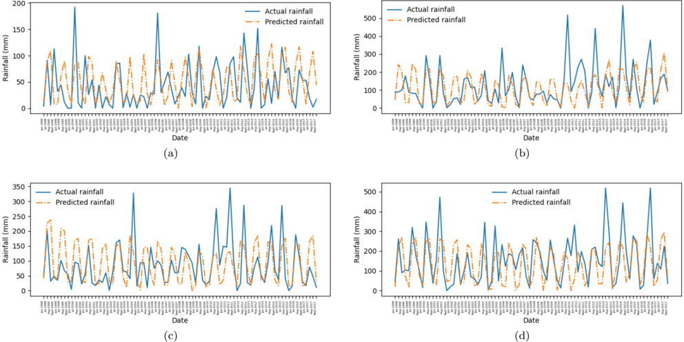
As mentioned in Section 2.1, Rajasthan is divided into four atmospheric zones, each of which having huge difference in their climatic and physiographic properties. To evaluate the effectiveness and accuracy of the proposed model, we apply it on each zone separately. The prediction results on one of the randomly picked rain-gauge stations from each zone is given in Table 2 and graphical representation is shown in Figure 5. Here we have used station data from WRD.
Table 2: Prediction results of DWMRPM on the four rain-gauge stations from WRDdataset. Each station is randomly picked from four different atmospheric zones.
| Zone Name | Latitude | Longitude | June | June | July | July | August | August | September | September |
|------------------------------|------------|-------------|--------|--------|--------|---------|----------|----------|-------------|-------------|
| Zone Name | Latitude | Longitude | MAE | RMSE | MAE | RMSE | MAE | RMSE | MAE | RMSE |
| North-West Desert | 29 ◦ 12'N | 73 ◦ 14'E | 2.4164 | 2.7660 | 5.1061 | 5.8879 | 4.8080 | 5.6060 | 2.8041 | 3.3493 |
| Central Aravalli | 26 ◦ 04'N | 74 ◦ 46'E | 3.1414 | 3.7925 | 7.7769 | 9.2311 | 11.5339 | 13.3020 | 4.7901 | 6.8593 |
| Hill Region Eastern Plain | 26 ◦ 41'N | 75 ◦ 14'E | 3.1223 | 3.7269 | 6.5146 | 7.8600 | 9.5284 | 10.7145 | 2.8730 | 3.4377 |
| South-Eastern Plateau Region | 25 ◦ 18'N | 75 ◦ 57'E | 6.2528 | 7.5165 | 8.3010 | 10.3782 | 9.0789 | 10.7850 | 5.0400 | 5.8975 |
Table 3: Comparison of the proposed DWMRPM with one Dimensional Convolutional Neural Networks (1-DCNN) and Multilayer Perceptron (MLP) on WRD dataset using for each month of the monsoon season.
| Month | MLP | MLP | 1-DCNN | 1-DCNN | DWMRPM | DWMRPM |
|------------------|---------|---------|----------|----------|----------|----------|
| Month | RMSE | MAE | RMSE | MAE | RMSE | MAE |
| June | 7.0382 | 5.8610 | 7.7567 | 5.2118 | 6.550 | 4.550 |
| July | 12.3831 | 9.2600 | 14.2568 | 10.3249 | 11.0974 | 8.7081 |
| August | 15.4046 | 12.3992 | 15.4564 | 10.4677 | 13.7013 | 10.4781 |
| September | 8.1199 | 9.5221 | 7.9481 | 5.9679 | 6.5770 | 5.0796 |
| Overall Accuracy | 10.2014 | 7.0106 | 11.8901 | 7.9931 | 9.9637 | 7.2052 |
IMD gridded data is not used in this case because the dataset is generated by interpolation which may have biases and outliers [56, 50].
## 3.2.2 Generalization ability of DWMRPM
In order to verify generalization ability of our model, we use it for monsoon rainfall prediction in each zone separately. The prediction results for each zone, on the basis of two evaluation criteria i.e., MAE and RMSE (Section 3.1.2) on WRD dataset are shown in Table 2 and Figure 5.
It can be observed that a single model is working well in rainfall forecasting for different geographical conditions ranging from plains and plateaus to desserts and hills.
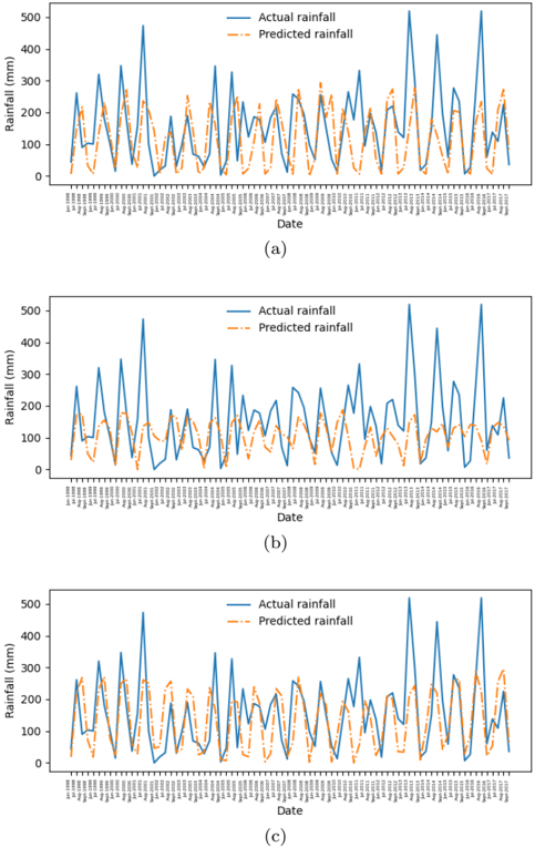
## 3.2.3 Comparison with baseline approaches
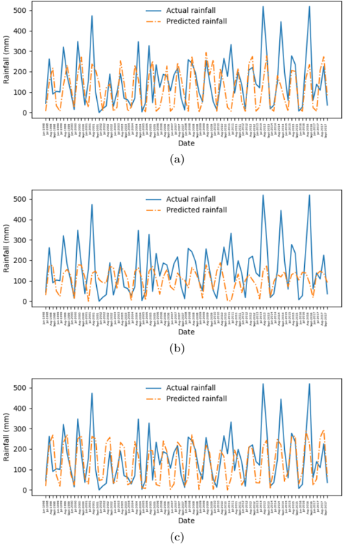
To establish the significance of present work, we compare the results of our model with the baseline approaches separately using the IMD gridded dataset and WRD station dataset.Table 3 and Table 4 show the comparison of the proposed DWMRPM with other approaches in the prediction of monsoon rainfall for the months of June, July, August and September on WRD and IMD datasets respectively. Overall accuracy of the model in the prediction of rainfall for the monsoon months is also given. Qualitative analysis for the comparison on different datasets is shown in Figure 6 and Figure 7
Fig. 5: Prediction results of DWMRPM for four rain-gauge stations, each picked from a different atmospheric zone (Section 3.2.2). Results are from year 2016 to 2017. (a) Prediction results of rain-gauge station situated at 29 ◦ 12'N, 73 ◦ 14'E in North-West dessert region, (b) Prediction results of raingauge station situated at 26 ◦ 04'N, 74 ◦ 46'E in Central Aravalli hill region, (c) Prediction results of rain-gauge station situated at 26 ◦ 41'N, 75 ◦ 14'E in Eastern plains region, and (d) Prediction results of rain-gauge station situated at 25 ◦ 18'N, 75 ◦ 57'E in South-Eastern plateau region.
<details>
<summary>Image 5 Details</summary>
### Visual Description
## Time Series Charts: Actual vs. Predicted Rainfall
### Overview
The image contains four time series charts, labeled (a), (b), (c), and (d), each displaying "Actual rainfall" and "Predicted rainfall" over time. The x-axis represents the date, and the y-axis represents rainfall in millimeters (mm). The charts show variations in rainfall patterns over a period of approximately 20 years.
### Components/Axes
* **Y-axis (Rainfall (mm))**:
* Chart (a): Scale from 0 to 200 mm, with markers at 0, 50, 100, 150, and 200.
* Chart (b): Scale from 0 to 500 mm, with markers at 0, 100, 200, 300, 400, and 500.
* Chart (c): Scale from 0 to 350 mm, with markers at 0, 50, 100, 150, 200, 250, 300, and 350.
* Chart (d): Scale from 0 to 500 mm, with markers at 0, 100, 200, 300, 400, and 500.
* **X-axis (Date)**: The x-axis represents time, with tick marks for each month, spanning from approximately January 1998 to September 2017.
* **Legend**: Located at the top of each chart.
* "Actual rainfall": Represented by a solid blue line.
* "Predicted rainfall": Represented by a dashed orange line.
* **Chart Labels**: Located at the bottom center of each chart: (a), (b), (c), and (d).
### Detailed Analysis
**Chart (a)**:
* **Actual Rainfall (Blue)**: The actual rainfall fluctuates, with several peaks. A notable peak occurs around 1998, reaching approximately 180 mm. The rainfall generally varies between 0 and 100 mm, with occasional spikes.
* **Predicted Rainfall (Orange)**: The predicted rainfall generally follows the trend of the actual rainfall but often underestimates the peak values. It also shows fluctuations, with values generally between 0 and 75 mm.
**Chart (b)**:
* **Actual Rainfall (Blue)**: The actual rainfall shows significant peaks, with one around 2002 reaching approximately 480 mm. The rainfall varies significantly, with values ranging from near 0 to almost 500 mm.
* **Predicted Rainfall (Orange)**: The predicted rainfall follows the general trend of the actual rainfall but tends to underestimate the higher peaks. It fluctuates between approximately 0 and 250 mm.
**Chart (c)**:
* **Actual Rainfall (Blue)**: The actual rainfall shows fluctuations, with peaks around 2000 and 2011, reaching approximately 320 mm and 280 mm, respectively. The rainfall varies between 0 and 320 mm.
* **Predicted Rainfall (Orange)**: The predicted rainfall follows the trend of the actual rainfall but often underestimates the peak values. It fluctuates between approximately 0 and 200 mm.
**Chart (d)**:
* **Actual Rainfall (Blue)**: The actual rainfall shows fluctuations, with peaks around 2002 and 2016, reaching approximately 480 mm and 450 mm, respectively. The rainfall varies between 0 and 500 mm.
* **Predicted Rainfall (Orange)**: The predicted rainfall follows the general trend of the actual rainfall but tends to underestimate the higher peaks. It fluctuates between approximately 0 and 300 mm.
### Key Observations
* The actual rainfall data exhibits significant variability across all four charts.
* The predicted rainfall generally follows the trend of the actual rainfall but often underestimates the peak values.
* The time period covered in each chart is approximately from January 1998 to September 2017.
* The y-axis scales differ across the charts, indicating potentially different regions or data sets.
### Interpretation
The charts compare actual rainfall data with predicted rainfall, likely from a predictive model. The consistent underestimation of peak rainfall values by the model suggests that the model may need refinement to better capture extreme weather events. The variations in rainfall patterns across the charts could be due to geographical differences or different data sources. The data suggests that while the model captures the general trend of rainfall, it struggles to accurately predict the magnitude of peak rainfall events. This could have implications for water resource management, flood prediction, and other related applications.
</details>
## 4 Conclusion and Future Work
This paper has presented a deep and wide neural network based model for the prediction of Rajasthan Summer Monsoon Rainfall (RSMR). Rainfall data is collected from Water Resource Department, Rajasthan and gridded data of resolution 0.25 X 0.25 degrees from Indian Meteorological Department (IMD). This model has the added advantage of exploiting the benefits from both the interpolated gridded data set and the unbiased single point station data set as well. Results obtained by DWRM are compared with baseline approaches like MLP and CNN. It is observed that for RSMR, the deep and wide model works better than other approaches. In future we may apply similar technique for the prediction of summer monsoon rainfall in other states in India as well
Table 4: Comparison of the proposed DWMRPM with one Dimensional Convolutional Neural Networks (1-DCNN) and Multi-layer Perceptron (MLP) on IMD dataset using for each month of the monsoon season.
| Month | MLP | MLP | 1-DCNN | 1-DCNN | DWMRPM | DWMRPM |
|------------------|---------|---------|----------|----------|----------|----------|
| Month | RMSE | MAE | RMSE | MAE | RMSE | MAE |
| June | 6.8156 | 5.7843 | 5.9660 | 5.0429 | 4.0239 | 3.1371 |
| July | 12.9685 | 9.9012 | 12.7962 | 8.5378 | 11.7024 | 7.8652 |
| August | 13.8754 | 12.8701 | 13.3874 | 12.6042 | 12.6878 | 12.1112 |
| September | 6.5700 | 5.8955 | 4.6474 | 4.52739 | 3.8953 | 4.0184 |
| Overall Accuracy | 11.5009 | 8.4529 | 9.5039 | 4.6780 | 9.0598 | 4.2830 |
as abroad. We plan to add more number of rainfall indicators and explore the possibilities of improving the accuracy of the current method.
## 5 Acknowledgments
This work is in collaboration with Water Resources, Government of Rajasthan. We are thankful to Indian Meteorological Department (IMD) and Special Project Monitoring Unit, National Hydrology Project, Water Resources Rajasthan, Jaipur, India for providing us the Rainfall data for this study.
## 6 Declaration
Funding:
Not Applicable
Conflicts of interest/Competing interests: The authors certify that they have NO affiliations with or involvement in any organization or entity with any financial interest or non-financial interest in the subject matter or materials discussed in this manuscript.
Availability of data and material: Available on request.
## References
1. Abadi M, Barham P, Chen J, Chen Z, Davis A, Dean J, Devin M, Ghemawat S, Irving G, Isard M, et al. (2016) Tensorflow: A system for largescale machine learning. In: 12th { USENIX } symposium on operating systems design and implementation ( { OSDI } 16), pp 265-283
2. Ancy S, Kumar R, Asokan R, Subhashini R (2014) Prediction of onset of south west monsoon using multiple regression. In: Proceedings of IEEE International Conference on Computer Communication and Systems ICCCS14, IEEE, pp 170-175
3. Bajpai V, Bansal A, Verma K, Agarwal S (2020) Prediction of rainfall in Rajasthan, India using deep and wide neural network. 2010.11787
Fig. 6: Comparison of DWMRPM and two deep-learning approaches on WRD dataset for a randomly selected rain-gauge station situated at 25 ◦ 18'N, 75 ◦ 57'E. The results are for the months of June, July, August and September of 20 years (June 1998 to September 2017) (a) Prediction results of MLP, (b) Prediction results of one dimensional CNN and, (d) Prediction results of the proposed DWMRPM.
<details>
<summary>Image 6 Details</summary>
### Visual Description
## Rainfall Prediction Comparison Charts
### Overview
The image presents three line charts, labeled (a), (b), and (c), comparing actual rainfall data with predicted rainfall data over time. Each chart spans a period from approximately January 1998 to September 2017. The y-axis represents rainfall in millimeters (mm), ranging from 0 to 500. The x-axis represents the date. The actual rainfall is represented by a solid blue line, while the predicted rainfall is represented by a dashed orange line.
### Components/Axes
* **Y-axis (Rainfall):**
* Label: "Rainfall (mm)"
* Scale: 0 to 500 mm, with implied increments of 100 mm.
* **X-axis (Date):**
* Label: "Date"
* Scale: Approximately January 1998 to September 2017. Tick marks are present for each month, but the month labels are only partially legible.
* **Legend:** Located in the top-right corner of each chart.
* "Actual rainfall" - Solid blue line
* "Predicted rainfall" - Dashed orange line
* **Chart Labels:** (a), (b), and (c) are located below each respective chart.
### Detailed Analysis
**Chart (a):**
* **Actual Rainfall (Blue):** The actual rainfall fluctuates significantly throughout the period. There are several peaks exceeding 400 mm, with the highest peak around 480 mm occurring around 2001. The trend is cyclical, with periods of high rainfall followed by periods of lower rainfall.
* **Predicted Rainfall (Orange):** The predicted rainfall generally follows the trend of the actual rainfall but with less extreme peaks and troughs. The predicted rainfall rarely exceeds 300 mm.
* **Data Points:**
* Jan 1998: Actual ~100 mm, Predicted ~50 mm
* 2001 Peak: Actual ~480 mm, Predicted ~250 mm
* Sept 2017: Actual ~150 mm, Predicted ~100 mm
**Chart (b):**
* **Actual Rainfall (Blue):** Similar to chart (a), the actual rainfall fluctuates significantly. A notable peak reaches approximately 470 mm around 2015.
* **Predicted Rainfall (Orange):** The predicted rainfall follows the general trend of the actual rainfall but with less intensity.
* **Data Points:**
* Jan 1998: Actual ~100 mm, Predicted ~50 mm
* 2015 Peak: Actual ~470 mm, Predicted ~250 mm
* Sept 2017: Actual ~150 mm, Predicted ~100 mm
**Chart (c):**
* **Actual Rainfall (Blue):** The actual rainfall shows similar fluctuations as in charts (a) and (b). A peak around 450 mm occurs around 2015.
* **Predicted Rainfall (Orange):** The predicted rainfall follows the trend of the actual rainfall, but the peaks are less pronounced.
* **Data Points:**
* Jan 1998: Actual ~100 mm, Predicted ~50 mm
* 2015 Peak: Actual ~450 mm, Predicted ~250 mm
* Sept 2017: Actual ~150 mm, Predicted ~100 mm
### Key Observations
* All three charts show similar patterns of actual and predicted rainfall.
* The predicted rainfall consistently underestimates the peak values of actual rainfall.
* The predicted rainfall generally captures the cyclical nature of the actual rainfall.
* The charts appear to represent different models or parameter settings for rainfall prediction.
### Interpretation
The charts illustrate the performance of rainfall prediction models. The models capture the overall trend of rainfall but struggle to accurately predict the magnitude of peak rainfall events. The differences between charts (a), (b), and (c) likely reflect variations in model parameters or model structure, leading to slightly different prediction outcomes. The consistent underestimation of peak rainfall suggests a limitation in the model's ability to capture extreme weather events. Further analysis would be needed to determine which model configuration (a, b, or c) provides the best overall performance based on metrics such as root mean squared error or correlation coefficient.
</details>
4. Bandyopadhyay A, Nengzouzam G, Singh WR, Hangsing N, Bhadra A (2018) Comparison of various re-analyses gridded data with observed data from meteorological stations over india. EPiC Series in Engineering 3:190198
Fig. 7: Comparison of DWMRPM and two deep-learning approaches on IMD dataset for a randomly coordinates situated at 25 ◦ 25'N, 75 ◦ 50'E. The results are for the months of June, July, August and September of 23 years (June 1996 to September 2018) (a) Prediction results of MLP, (b) Prediction results of one dimensional CNN and, (d) Prediction results of the proposed DWMRPM.
<details>
<summary>Image 7 Details</summary>
### Visual Description
## Time Series Chart: Actual vs. Predicted Rainfall
### Overview
The image presents three time series charts comparing actual rainfall to predicted rainfall over different time periods. Each chart displays two lines: a solid blue line representing the actual rainfall and a dashed orange line representing the predicted rainfall. The x-axis represents time (Date), and the y-axis represents rainfall in millimeters (mm). The three charts cover different time spans, with the first chart (a) spanning from approximately January 1998 to January 2011, the second chart (b) spanning from approximately January 2003 to January 2017, and the third chart (c) spanning from approximately January 1998 to January 2017.
### Components/Axes
* **Y-axis:** Rainfall (mm), ranging from 0 to 500 in all three charts.
* **X-axis:** Date, with varying start and end dates for each chart.
* Chart (a): Approximately Jan 1998 to Jan 2011
* Chart (b): Approximately Jan 2003 to Jan 2017
* Chart (c): Approximately Jan 1998 to Jan 2017
* **Legend:** Located in the top-right corner of each chart.
* Blue solid line: "Actual rainfall"
* Orange dashed line: "Predicted rainfall"
* **Titles:** Each chart is labeled with a letter in parentheses: (a), (b), and (c).
### Detailed Analysis
**Chart (a): Jan 1998 - Jan 2011**
* **Actual Rainfall (Blue):** The actual rainfall fluctuates significantly over time, with peaks reaching approximately 400-500 mm and troughs near 0 mm. There is a general cyclical pattern, suggesting seasonal variations.
* **Predicted Rainfall (Orange):** The predicted rainfall generally follows the trend of the actual rainfall but tends to underestimate the peak values. The predicted rainfall also shows a cyclical pattern, but the amplitude of the fluctuations is smaller than that of the actual rainfall.
* Example Data Points:
* Around 2001, Actual Rainfall peaks at approximately 400 mm, while Predicted Rainfall peaks at approximately 250 mm.
* Around 2008, Actual Rainfall peaks at approximately 350 mm, while Predicted Rainfall peaks at approximately 200 mm.
**Chart (b): Jan 2003 - Jan 2017**
* **Actual Rainfall (Blue):** Similar to chart (a), the actual rainfall fluctuates significantly, with peaks reaching approximately 400-500 mm and troughs near 0 mm.
* **Predicted Rainfall (Orange):** The predicted rainfall follows the trend of the actual rainfall but underestimates the peak values.
* Example Data Points:
* Around 2005, Actual Rainfall peaks at approximately 480 mm, while Predicted Rainfall peaks at approximately 200 mm.
* Around 2013, Actual Rainfall peaks at approximately 350 mm, while Predicted Rainfall peaks at approximately 250 mm.
**Chart (c): Jan 1998 - Jan 2017**
* **Actual Rainfall (Blue):** The actual rainfall fluctuates significantly, with peaks reaching approximately 400-500 mm and troughs near 0 mm.
* **Predicted Rainfall (Orange):** The predicted rainfall follows the trend of the actual rainfall but underestimates the peak values.
* Example Data Points:
* Around 2001, Actual Rainfall peaks at approximately 400 mm, while Predicted Rainfall peaks at approximately 250 mm.
* Around 2013, Actual Rainfall peaks at approximately 350 mm, while Predicted Rainfall peaks at approximately 250 mm.
### Key Observations
* The predicted rainfall consistently underestimates the actual rainfall peaks in all three charts.
* The cyclical pattern of rainfall is captured by the predicted rainfall, but the magnitude of the predicted rainfall variations is smaller than the actual rainfall variations.
* The charts show that the model used for prediction captures the general trend of rainfall but needs improvement in accurately predicting the peak rainfall values.
### Interpretation
The charts demonstrate the performance of a rainfall prediction model over different time periods. The model captures the overall trend and seasonality of rainfall but tends to underestimate the peak values. This could be due to various factors, such as limitations in the model's complexity, the quality of the input data, or the presence of unpredictable weather events. The underestimation of peak rainfall could have significant implications for applications such as flood forecasting and water resource management, where accurate prediction of extreme events is crucial. Further refinement of the prediction model is needed to improve its accuracy, particularly in predicting peak rainfall values. The similarity between the charts suggests that the model's performance is consistent across different time periods.
</details>
5. Bokil M (2000) Drought in rajasthan: In search of a perspective. Economic and Political Weekly pp 4171-4175
6. Bryson RA, Swain A (1981) Holocene variations of monsoon rainfall in rajasthan. Quaternary Research 16(2):135-145
7. Campling P, Gobin A, Feyen J (2001) Temporal and spatial rainfall analysis across a humid tropical catchment. Hydrological processes 15(3):359-
8. Chakraverty S, Gupta P (2008) Comparison of neural network configurations in the long-range forecast of southwest monsoon rainfall over india. Neural Computing and Applications 17(2):187-192
9. Cheng HT, Koc L, Harmsen J, Shaked T, Chandra T, Aradhye H, Anderson G, Corrado G, Chai W, Ispir M, Anil R, Haque Z, Hong L, Jain V, Liu X, Shah H (2016) Wide & deep learning for recommender systems. In: Proceedings of the 1st Workshop on Deep Learning for Recommender Systems, p 7-10
10. Cheng HT, Koc L, Harmsen J, Shaked T, Chandra T, Aradhye H, Anderson G, Corrado G, Chai W, Ispir M, et al. (2016) Wide & deep learning for recommender systems. In: Proceedings of the 1st workshop on deep learning for recommender systems, pp 7-10
11. Chollet F, et al. (2015) Keras. URL https://github.com/fchollet/ keras
12. Clift PD, Plumb RA (2008) The Asian monsoon: causes, history and effects, vol 288. Cambridge University Press Cambridge
13. Dash Y, Mishra SK, Sahany S, Panigrahi BK (2018) Indian summer monsoon rainfall prediction: a comparison of iterative and non-iterative approaches. Applied Soft Computing 70:1122-1134
14. Dubey AD (2015) Artificial neural network models for rainfall prediction in pondicherry. International Journal of Computer Applications 120(3)
15. Ducrocq V, Ricard D, Lafore JP, Orain F (2002) Storm-scale numerical rainfall prediction for five precipitating events over france: On the importance of the initial humidity field. Weather and Forecasting 17(6):12361256
16. Dutta D, Kundu A, Patel N (2013) Predicting agricultural drought in eastern rajasthan of india using ndvi and standardized precipitation index. Geocarto International 28(3):192-209
17. Dutta S, Chaudhuri G (2015) Evaluating environmental sensitivity of arid and semiarid regions in northeastern rajasthan, india. Geographical Review 105(4):441-461
18. Enzel Y, Ely LL, Mishra S, Ramesh R, Amit R, Lazar B, Rajaguru S, Baker V, Sandler A (1999) High-resolution holocene environmental changes in the thar desert, northwestern india. Science 284(5411):125-128
19. Fan L, Shin SI, Liu Q, Liu Z (2013) Relative importance of tropical sst anomalies in forcing east asian summer monsoon circulation. Geophysical Research Letters 40(10):2471-2477
20. Gadgil S, Srinivasan J, Nanjundiah RS, Kumar KK, Munot A, Kumar KR (2002) On forecasting the indian summer monsoon: the intriguing season of 2002. Current Science 83(4):394-403
21. Gadgil S, Rajeevan M, Nanjundiah R (2005) Monsoon prediction - why yet another failure? Current Science 88(9):1389-1400, URL http://www. jstor.org/stable/24110705
22. Glorot X, Bengio Y (2010) Understanding the difficulty of training deep feedforward neural networks. In: In Proceedings of the International Con-
- ference on Artificial Intelligence and Statistics (AISTATS'10). Society for Artificial Intelligence and Statistics, pp 249-256
23. Goel A, Singh R (2006) Climatic variability and drought in rajasthan. In: Advances in Geosciences: Volume 4: Hydrological Science (HS), World Scientific, pp 57-67
24. Goyal HR, Ghanshala KK, Sharma S (2021) Recommendation based rescue operation model for flood victim using smart iot devices. Materials Today: Proceedings
25. Gu J, Wang Z, Kuen J, Ma L, Shahroudy A, Shuai B, Liu T, Wang X, Wang G, Cai J, et al. (2018) Recent advances in convolutional neural networks. Pattern Recognition 77:354-377
26. Gulli A, Pal S (2017) Deep learning with Keras. Packt Publishing Ltd
27. Halbe J, Pahl-Wostl C, Sendzimir J, Adamowski J (2013) Towards adaptive and integrated management paradigms to meet the challenges of water governance. Water Science and Technology 67(11):2651-2660
28. He J, Wen M, Wang L, Xu H (2006) Characteristics of the onset of the asian summer monsoon and the importance of asian-australian 'land bridge'. Advances in Atmospheric Sciences 23(6):951-963
29. He K, Zhang X, Ren S, Sun J (2015) Delving deep into rectifiers: Surpassing human-level performance on imagenet classification. In: Proceedings of the 2015 IEEE International Conference on Computer Vision (ICCV), p 1026-1034
30. He K, Zhang X, Ren S, Sun J (2015) Delving deep into rectifiers: Surpassing human-level performance on imagenet classification. In: Proceedings of the IEEE international conference on computer vision, pp 1026-1034
31. Jang J, Han S (2011) Importance of monsoon rainfall in mass fluxes of filtered and unfiltered mercury in gwangyang bay, korea. Science of the total environment 409(8):1498-1503
32. Johny K, Pai ML, Adarsh S (2020) Adaptive eemd-ann hybrid model for indian summer monsoon rainfall forecasting. Theoretical and Applied Climatology pp 1-17
33. Kalsi S, Hatwar H, Jayanthi N, Subramanian S, Shyamala B, Rajeevan M, Jenamani R (2004) Various aspects of unusual behaviour of monsoon 2002. India Meteorol Dep Monogr 2:97
34. KARAN D (2016) An empirical study of impact of drought on agricultural produce and use of inputs in rajasthan. EIJFMR
35. Kerhoulas LP, Kolb TE, Koch GW (2017) The influence of monsoon climate on latewood growth of southwestern ponderosa pine. Forests 8(5):140
36. Kim M, Lee S, Kim J (2020) A wide & deep learning sharing input data for regression analysis. In: 2020 IEEE International Conference on Big Data and Smart Computing (BigComp), IEEE, pp 8-12
37. Kingma DP, Ba J (2014) Adam: A method for stochastic optimization. arXiv preprint arXiv:14126980
38. Kulshreshtha S, Sharma S, Sharma B (2013) The majestic rajasthan: an introduction. In: Faunal heritage of Rajasthan, India, Springer, pp 3-37
39. Lal Meena A, Bisht P, et al. (2020) Study of rainfall pattern in chaksu tehsil, jaipur, rajasthan, india
40. Lau KM, Li MT (1984) The monsoon of east asia and its global associations-a survey. Bulletin of the American Meteorological Society 65(2):114-125
41. Li M, Shao Q (2010) An improved statistical approach to merge satellite rainfall estimates and raingauge data. Journal of Hydrology 385(1-4):5164
42. Meena HM, Machiwal D, Santra P, Moharana PC, Singh D (2019) Trends and homogeneity of monthly, seasonal, and annual rainfall over arid region of rajasthan, india. Theoretical and Applied Climatology 136(3):795-811
43. Meher JK, Das L (2019) Gridded data as a source of missing data replacement in station records. Journal of Earth System Science 128(3):1-14
44. Montanari A, Grossi G (2008) Estimating the uncertainty of hydrological forecasts: A statistical approach. Water Resources Research 44(12)
45. Mooley D (1997) Variation of summer monsoon rainfall over india in eini˜ nos
46. Mooley D, Parthasarathy B (1984) Fluctuations in all-india summer monsoon rainfall during 1871-1978. Climatic change 6(3):287-301
47. Mundetia N, Sharma D, et al. (2015) Analysis of rainfall and drought in rajasthan state, india. Global Nest J 17(1):12-21
48. Naidu C, Durgalakshmi K, Muni Krishna K, Ramalingeswara Rao S, Satyanarayana G, Lakshminarayana P, Malleswara Rao L (2009) Is summer monsoon rainfall decreasing over india in the global warming era? Journal of Geophysical Research: Atmospheres 114(D24)
49. Ng A, et al. (2011) Sparse autoencoder. CS294A Lecture notes 72(2011):119
50. Pai D, Sridhar L, Rajeevan M, Sreejith O, Satbhai N, Mukhopadhyay B (2014) Development of a new high spatial resolution (0.25 × 0.25) long period (1901-2010) daily gridded rainfall data set over india and its comparison with existing data sets over the region. Mausam 65(1):1-18
51. Pal SK, Mitra S (1992) Multilayer perceptron, fuzzy sets, classifiaction
52. Parthasarathy B, Sontakke N, Monot A, Kothawale D (1987) Droughts/floods in the summer monsoon season over different meteorological subdivisions of india for the period 1871-1984. Journal of Climatology 7(1):57-70
53. Parthasarathy B, Munot A, Kothawale D (1988) Regression model for estimation of indian foodgrain production from summer monsoon rainfall. Agricultural and Forest Meteorology 42(2-3):167-182
54. Pingale SM, Khare D, Jat MK, Adamowski J (2014) Spatial and temporal trends of mean and extreme rainfall and temperature for the 33 urban centers of the arid and semi-arid state of rajasthan, india. Atmospheric Research 138:73-90
55. Preethi B, Revadekar J, Kripalani R (2011) Anomalous behaviour of the indian summer monsoon 2009. Journal of earth system science 120(5):783794
56. Rajeevan M, Bhate J, Kale J, Lal B (2005) Development of a high resolution daily gridded rainfall data for the indian region. Met Monograph Climatology 22:2005
57. Ray K, Pandey P, Pandey C, Dimri A, Kishore K (2019) On the recent floods in india. Current science 117(2):204-218
58. Ren L, Meng Z, Wang X, Lu R, Yang LT (2020) A wide-deep-sequence model-based quality prediction method in industrial process analysis. IEEE Transactions on Neural Networks and Learning Systems 31(9):37213731
59. Roy AB, Jakhar SR (2002) Geology of Rajasthan (Northwest India) precambrian to recent. Scientific Publishers
60. Saha M, Mitra P, Nanjundiah RS (2016) Autoencoder-based identification of predictors of indian monsoon. Meteorology and Atmospheric Physics 128(5):613-628
61. Saha M, Santara A, Mitra P, Chakraborty A, Nanjundiah RS (2021) Prediction of the indian summer monsoon using a stacked autoencoder and ensemble regression model. International Journal of Forecasting 37(1):5871
62. Sahai A, Soman M, Satyan V (2000) All india summer monsoon rainfall prediction using an artificial neural network. Climate dynamics 16(4):291302
63. Shanker M, Hu MY, Hung MS (1996) Effect of data standardization on neural network training. Omega 24(4):385-397
64. Sikka D (2003) Evaluation of monitoring and forecasting of summer monsoon over india and a review of monsoon drought of 2002. ProceedingsIndian National Science Academy Part A 69(5):479-504
65. Singh A, Kulkarni MA, Mohanty U, Kar S, Robertson AW, Mishra G (2012) Prediction of indian summer monsoon rainfall (ismr) using canonical correlation analysis of global circulation model products. Meteorological Applications 19(2):179-188
66. Singh B, Rajpurohit D, Vasishth A, Singh J (2012) Probability analysis for estimation of annual one day maximum rainfall of jhalarapatan area of rajasthan, india. Plant Archives 12(2):1093-1100
67. Singh P (2016) Applications of soft computing in time series forecasting. Springer
68. Singh P (2018) Indian summer monsoon rainfall (ismr) forecasting using time series data: A fuzzy-entropy-neuro based expert system. Geoscience Frontiers 9(4):1243-1257
69. Singh P (2018) Rainfall and financial forecasting using fuzzy time series and neural networks based model. International Journal of Machine Learning and Cybernetics 9(3):491-506
70. Singh P, Borah B (2013) Indian summer monsoon rainfall prediction using artificial neural network. Stochastic environmental research and risk assessment 27(7):1585-1599
71. Swaminathan M (1998) Padma bhusan prof. P Koteswaram First Memorial Lecture-23rd March pp 3-10
72. Tierney JE, Russell JM, Damst´ e JSS, Huang Y, Verschuren D (2011) Late quaternary behavior of the east african monsoon and the importance of the congo air boundary. Quaternary Science Reviews 30(7-8):798-807
73. Upadhyaya H (2014) Vulnerability and adaptation to climate change in the context of water resource with reference to rajasthan. PhD thesis, The IIS University
74. Van SP, Le HM, Thanh DV, Dang TD, Loc HH, Anh DT (2020) Deep learning convolutional neural network in rainfall-runoff modelling. Journal of Hydroinformatics 22(3):541-561
75. Walker GT (1933) Seasonal weather and its prediction
76. Yadav SK, Nath S, Gautam S (2018) Analysis of rainfall variability in western rajasthan, india. Journal of Pharmacognosy and Phytochemistry 7(4):1592-1595
77. Yadav SM, Mangukiya NK (2021) Semi-arid river basin flood: Causes, damages, and measures. In: Proceedings of the Fifth International Conference in Ocean Engineering (ICOE2019), Springer, pp 201-212
78. Zhang G, Eddy Patuwo B, Y Hu M (1998) Forecasting with artificial neural networks:: The state of the art. International Journal of Forecasting 14(1):35-62