## Generalized Planning as Heuristic Search
1 Javier Segovia-Aguas, 2 Sergio Jim´ enez and 1 Anders Jonsson
1 Dept. Information and Communication Technologies, Universitat Pompeu Fabra, Spain
2 VRAIN - Valencian Research Institute for Artificial Intelligence, Universitat Polit` ecnica de Val` encia, Spain javier.segovia@upf.edu, serjice@dsic.upv.es, anders.jonsson@upf.edu
## Abstract
Although heuristic search is one of the most successful approaches to classical planning, this planning paradigm does not apply straightforwardly to Generalized Planning (GP). Planning as heuristic search traditionally addresses the computation of sequential plans by searching in a grounded statespace. On the other hand GP aims at computing algorithmlike plans, that can branch and loop, and that generalize to a (possibly infinite) set of classical planning instances. This paper adapts the planning as heuristic search paradigm to the particularities of GP, and presents the first native heuristic search approach to GP. First, the paper defines a novel GP solution space that is independent of the number of planning instances in a GP problem, and the size of these instances. Second, the paper defines different evaluation and heuristic functions for guiding a combinatorial search in our GP solution space. Lastly the paper defines a GP algorithm, called Best-First Generalized Planning (BFGP), that implements a best-first search in the solution space guided by our evaluation/heuristic functions.
## Introduction
Heuristic search is one of the most successful approaches to classical planning (Bonet and Geffner 2001; Hoffmann 2001; Helmert 2006; Richter and Westphal 2010; Lipovetzky and Geffner 2017). Unfortunately, it is not straightforward to adopt state-of-the-art search algorithms and heuristics from classical planning to Generalized Planning (GP). The planning as heuristic search approach traditionally addresses the computation of sequential plans with a grounded state-space search. Generalized planners reason however about the synthesis of algorithm-like solutions that, in addition to action sequences, contain branching and looping constructs. Furthermore, GP aims to synthesize solutions that generalize to a (possibly infinite) set of planning instances (where the domain of variables may be large), making the grounding of classical planners unfeasible (Winner and Veloso 2003; Hu and Levesque 2011; Siddharth et al. 2011; Hu and De Giacomo 2013; Bonet, Frances, and Geffner 2019; Illanes and McIlraith 2019).
Copyright © 2021, Association for the Advancement of Artificial Intelligence (www.aaai.org). All rights reserved.
This paper adapts the planning as heuristic search paradigm to the particularities of GP, and presents the first native heuristic search approach to GP. Given a GP problem, that comprises an input set of classical planning instances from a given domain, our GP as heuristic search approach computes an algorithm-like plan that solves the full set of input instances. The contributions of the paper are three-fold:
1. A tractable solution space for GP . We leverage the computational models of the Random-Access Machine (Skiena 1998) and the Intel x86 FLAGS register (Dandamudi 2005) to define an innovative solution space that is independent of the number of input planning instances in a GP problem, and the size of these instances (i.e. the number of state variables and their domain size).
2. Grounding-free evaluation/heuristic functions for GP. We define several evaluation and heuristic functions to guide a combinatorial search in our GP solution space. Evaluating these functions does not require to ground states/actions in advance, so they allow to address GP problems where state variables have large domains (e.g. integers).
3. A heuristic search algorithm for GP . We present the BFGP algorithm that implements a best-first search in our GP solution space. Experiments show that BFGP significantly reduces the CPU-time required to compute and validate generalized plans, compared to the classical planning compilation approach to GP (Segovia-Aguas, Jim´ enez, and Jonsson 2019).
## Background
This section introduces the necessary notation to define our heuristic search approach to generalized planning.
## Classical Planning
Let X be a set of state variables , each x ∈ X with domain D x . A state is a total assignment of values to the set of state variables, i.e. 〈 x 0 = v 0 , . . . , x N = v N 〉 such that for every x i ∈ X then v i ∈ D x i . For a variable subset X ′ ⊆ X , let D [ X ′ ] = × x ∈ X ′ D x denote its joint domain. The state space is then S = D [ X ] . Given a state s ∈ S and a subset of variables X ′ ⊆ X , let s | X ′ = 〈 x i = v i 〉 x i ∈ X ′ be the projection of s onto X ′ i.e. the partial state defined by the values that s assigns to the variables in X ′ . The projection of s onto X ′ defines the subset of states { s | s ∈ S, s | X ′ ⊆ s } that are consistent with the corresponding partial state.
Let A be a set of deterministic lifted actions . A lifted action a ∈ A has an associated set of variables par ( a ) ⊆ X , called parameters , and is characterized by two functions: an applicability function ρ a : D [ par ( a )] → { 0 , 1 } , and a successor function θ a : D [ par ( a )] → D [ par ( a )] . Action a is applicable in a given state s iff ρ a ( s | par ( a ) ) equals 1 , and results in a successor state s ′ = s ⊕ a , that is built replacing the values that s assigns to variables in par ( a ) with the values specified by θ a ( s | par ( a ) ) . Lifted actions generalize actions with conditional effects . These actions are common in GP since their state-dependent outcomes allow to adapt generalized plans to different classical planning instances.
A classical planning instance is a tuple P = 〈 X,A,I,G 〉 , where X is a set of state variables, A is a set of lifted actions, I ∈ S is an initial state, and G is a goal condition on the state variables that induces the subset of goal states S G = { s | s /satisfies G,s ∈ S } . Given P , a plan is an action sequence π = 〈 a 1 , . . . , a m 〉 whose execution induces a trajectory τ = 〈 s 0 , a 1 , s 1 , . . . , a m , s m 〉 such that, for each 1 ≤ i ≤ m , a i is applicable in s i -1 and results in the successor state s i = s i -1 ⊕ a i . A plan π solves P if the execution of π in s 0 = I finishes in a goal state, i.e. s m ∈ S G . We say π is optimal if | π | = m is minimal among the plans that solve P .
## Generalized Planning
Generalized planning is an umbrella term that refers to more general notions of planning (Jim´ enez, Segovia-Aguas, and Jonsson 2019). This work builds on top of the inductive formalism for GP, where a GP problem is defined as a set of classical planning instances with a common structure.
Definition 1 (GP problem with shared state variables) . A GP problem is a finite and non-empty set of T classical planning instances P = { P 1 , . . . , P T } , where each classical planning instance P t ∈ P , 1 ≤ t ≤ T , shares the same sets of state variables X and lifted actions A , but may differ in the initial state and goals. Formally, P 1 = 〈 X,A,I 1 , G 1 〉 , . . . , P T = 〈 X,A,I T , G T 〉 .
The representations of GP solutions range from programs (Winner and Veloso 2003; Segovia-Aguas, Jim´ enez, and Jonsson 2019) and generalized policies (Mart´ ın and Geffner 2004; Franc` es Medina et al. 2019), to finite state controllers (Bonet, Palacios, and Geffner 2010; Segovia-Aguas, Jim´ enez, and Jonsson 2016), formal grammars or hierarchies (Nau et al. 2003; Ramirez and Geffner 2016; Segovia-Aguas, Jim´ enez, and Jonsson 2017). Each representation has its own expressiveness capacity, as well as its own validation/computation complexity. We can however define a common condition under which a generalized plan is considered a solution to a GP problem. First, let us define exec (Π , P ) = 〈 a 1 , . . . , a m 〉 as the sequential plan produced by the execution of a generalized plan Π , on a classical planning instance P = 〈 X,A,I,G 〉 .
Definition 2 (GP solution) . A generalized plan Π solves a GP problem P = { P 1 , . . . , P T } iff, for every classical plan-
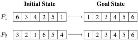
Figure 1: Classical planning instances for sorting the content of two six-element lists by swapping the list elements.
<details>
<summary>Image 1 Details</summary>
### Visual Description
\n
## Diagram: State Transition Illustration
### Overview
The image depicts a diagram illustrating the transition from an "Initial State" to a "Goal State" for two problems, labeled P1 and P2. Each problem is represented by a sequence of six numbered boxes, showing the arrangement of numbers within each state. An arrow indicates the transformation from the initial to the goal state.
### Components/Axes
The diagram is divided into two columns labeled "Initial State" and "Goal State". Each column contains two rows, labeled P1 and P2. Each row represents a problem instance. Within each row, there are six boxes representing the state of the problem. The boxes contain numerical values from 1 to 6. Arrows point from the initial state to the goal state.
### Detailed Analysis or Content Details
**Problem P1:**
* **Initial State:** The sequence of numbers is 6, 3, 4, 2, 5, 1.
* **Goal State:** The sequence of numbers is 1, 2, 3, 4, 5, 6.
**Problem P2:**
* **Initial State:** The sequence of numbers is 3, 2, 1, 6, 5, 4.
* **Goal State:** The sequence of numbers is 1, 2, 3, 4, 5, 6.
### Key Observations
Both problems (P1 and P2) share the same "Goal State" – a sequence of numbers arranged in ascending order from 1 to 6. The "Initial States" for both problems are different, representing different starting configurations. The diagram illustrates a transformation or a series of steps required to move from the initial disordered state to the final ordered state.
### Interpretation
This diagram likely represents a problem-solving scenario, potentially in the context of algorithms or search strategies. The "Initial State" represents the starting point of a problem, and the "Goal State" represents the desired solution. The arrow suggests a process or algorithm that transforms the initial state into the goal state. The fact that both problems converge to the same goal state suggests that the goal is well-defined and independent of the initial configuration. This could be a puzzle, a sorting problem, or a state-space search problem. The diagram doesn't provide information about *how* the transformation is achieved, only that it is possible. It is a visual representation of a before-and-after scenario.
</details>
ning instance P t ∈ P , 1 ≤ t ≤ T , it holds that exec (Π , P t ) solves P t .
We define the cost of a GP solution as the sum of the costs of the sequential plans that are produced for each of the classical planning instances in a GP problem. Formally, cost (Π , P ) = ∑ P t ∈P | exec (Π , P t ) | . A GP solution Π is optimal if cost (Π , P ) is minimal among the generalized plans that solve P .
Example . Figure 1 shows the initial state and goal of two instances, P 1 = 〈 X,A,I 1 , G 1 〉 and P 2 = 〈 X,A,I 2 , G 2 〉 , for sorting two six-element lists. Both instances share the set of state variables X = { x 1 , x 2 , x 3 , x 4 , x 5 , x 6 } that encode six integers. They also share the set of lifted actions A , with 6 × 5 2 swap ( x i , x j ) actions that swap the content of two list positions i < j . An example solution plan for P 1 is π 1 = 〈 swap ( x 1 , x 6 ) , swap ( x 2 , x 3 ) , swap ( x 2 , x 4 ) 〉 while π 2 = 〈 swap ( x 1 , x 3 ) , swap ( x 4 , x 6 ) 〉 is a solution for P 2 . The set P = { P 1 , P 2 } is an example GP problem. Sorting instances with different list sizes is made possible by including enough state variables to represent the elements of the longest list, and an extra state variable for the list length; e.g. length = l implies that list positions [0 , l -1] are valid.
## Planning Programs
In this work we represent GP solutions as planning programs (Segovia-Aguas, Jim´ enez, and Jonsson 2019). The execution of a planning program on a classical planning instance is a deterministic procedure that requires no variable matching; this is a useful property when implementing native heuristics for the space of GP solutions.
Formalization. A planning program is a sequence of n instructions Π = 〈 w 0 , . . . , w n -1 〉 , where each instruction w i ∈ Π is associated with a program line 0 ≤ i < n and is either:
- A planning action w i ∈ A .
- A goto instruction w i = go ( i ′ , ! y ) , where i ′ is a program line 0 ≤ i ′ < i or i +1 < i ′ < n , and y is a proposition.
- A termination instruction w i = end . The last instruction of a program Π is always w n -1 = end .
The execution model for a planning program is a program state ( s, i ) , i.e. a pair of a planning state s ∈ S and program counter 0 ≤ i < n . Given a program state ( s, i ) , the execution of a programmed instruction w i is defined as:
- If w i ∈ A , the new program state is ( s ′ , i + 1) , where s ′ = s ⊕ w i is the successor when applying w i in s .
- If w i = go ( i ′ , ! y ) , the new program state is ( s, i + 1) if y holds in s , and ( s, i ′ ) otherwise 1 . Proposition y can be the result of an arbitrary expression on state variables, e.g. high-level state features (Lotinac et al. 2016).
- If w i = end , program execution terminates.
To execute a planning program Π on a planning instance P = 〈 X,A,I,G 〉 , the initial program state is set to ( I, 0) , i.e. the initial state of P and the first program line of Π . A program Π solves P iff execution terminates in a program state ( s, i ) that satisfies the goal condition, i.e. w i = end and s ∈ S G . If a planning program fails to solve the instance, the only possible sources of failure are: (i) incorrect program , i.e. execution terminates in a program state ( s, i ) that does not satisfy the goal condition, i.e. ( w i = end ) ∧ ( s / ∈ S G ) ; (ii) inapplicable program , i.e. executing action w i ∈ A fails in program state ( s, i ) since w i is not applicable in s ; (iii) infinite program , i.e. execution enters into an infinite loop that never reaches an end instruction.
The space of planning programs. Given a maximum number of program lines n , where the last instruction is w n -1 = end , and defined the propositions of goto instructions as ( x = v ) atoms, where x ∈ X and v ∈ D x . The space of possible planning programs is compactly represented with three bit-vectors
1. The action vector of length ( n -1) × | A | , indicating whether action a ∈ A appears on line 0 ≤ i < n -1 .
2. The transition vector of length ( n -1) × ( n -2) , indicating whether go ( i ′ , ∗ ) appears on line 0 ≤ i < n -1 .
3. The proposition vector of length ( n -1) × ∑ x ∈ X | D x | , indicating if go ( ∗ , ! 〈 x = v 〉 ) appears on line 0 ≤ i < n -1 .
Aplanning program is encoded as the concatenation of these three bit-vectors. The length of the resulting vector is:
$$( n - 1 ) \left ( | A | + ( n - 2 ) + \sum _ { x \in X } | D _ { x } | \right ) . \quad ( 1 )$$
This encoding allows us to quantify the similarity of two planning programs (their Hamming distance ) and more importantly, to implement a combinatorial search in the space of planning programs with n lines. In fact, this is the encoding leveraged by the classical planning compilation approach to GP (Segovia-Aguas, Jim´ enez, and Jonsson 2019). Equation 1 reveals an important scalability limitation of this solution space that limits the applicability of the cited compilation to instances of small size: the number of planning programs with n lines depends on the number, and domain size, of the state variables.
## A Tractable Solution Space for GP
This section defines a scalable GP solution space of candidate planning programs , that is independent of the size of the input planning instances in a GP problem (i.e. the number of
1 We adopt the convention of jumping to line i ′ whenever y is false , inspired by jump instructions in the Random-Access Machine that jump when a register equals zero.
state variables and their domain size). Our approach is to extend the input classical planning instances of a GP problem with a general, and compact, feature language. This way the different classical planning instances in a given GP problem share a common set of features, even if their sets of states variables are actually different.
Our general and compact feature language leverages the computational model of the Random-Access Machine (RAM), an abstract computation machine that is polynomial-equivalent to a Turing machine (Boolos, Burgess, and Jeffrey 2002). The RAM machine enhances the counter machine with indirect memory addressing (Minsky 1961), and it allows augmented instruction sets and auxiliary dedicated registers, like the FLAGS register of the Intel x86 microprocessors (Dandamudi 2005).
## Classical Planning with Pointers
We extend the classical planning model with a RAM machine of | Z | + 2 registers: | Z | pointers that reference the original planning state variables, plus the zero and carry FLAGS (whose joint value will represent our common set of features for GP). Given a classical planning instance P = 〈 X,A,I,G 〉 , the extended classical planning instance with a RAM machine of | Z | + 2 registers is defined as P ′ Z = 〈 X ′ Z , A ′ Z , I ′ Z , G 〉 , where:
- The new set of state variables X ′ Z comprises:
- -The state variables X of the original planning instance.
- -Two Boolean variables Y = { y z , y c } , that play the role of the zero and carry FLAGS register.
- -The pointers Z , a non-empty set of extra state variables with finite domain [0 , . . . , | X | -1] .
- The new set of actions A ′ Z includes:
- -The planning actions A ′ that result from abstracting each original planning action a ∈ A into its corresponding action scheme. The abstraction is a two-step procedure that requires at least as many pointers as the largest arity of an action in A : (i), each action parameter is replaced with a pointer in Z (ii), its applicability/successor function is rewritten to refer to the state variables pointed by the action parameters. For instance, the 6 × 5 2 swap( x i , x j ) actions from the example of Figure 1, are abstracted into the action scheme { swap( z 1 , z 2 ) | z 1 , z 2 ∈ Z } using two pointers, Z = { z 1 , z 2 } .
- -The RAM actions that implement the following set of RAM instructions { inc ( z 1 ) , dec ( z 1 ) , cmp ( z 1 , z 2 ) , cmp ( ∗ z 1 , ∗ z 2 ) , set ( z 1 , z 2 ) | z 1 , z 2 ∈ Z } over the pointers in Z. Respectively, these RAM instructions increment/decrement a pointer, compare two pointers (or their content), and set the value of a pointer z 1 to another pointer z 2 . Each RAM action also updates the FLAGS Y = { y z , y c } , according to the result of the cor-
responding RAM instruction (denoted here by res ):
<!-- formula-not-decoded -->
The number of actions of a classical planning instance, extended with a RAM machine of | Z | +2 registers, is
$$| A _ { Z } ^ { \prime } | = 2 | Z | ^ { 2 } + | A ^ { \prime } | .$$
The increment / decrement instructions induce 2 | Z | actions, the set instructions over pointers induce | Z | 2 -| Z | actions, and comparison instructions induce | Z | 2 -| Z | actions; they can compare pointers or their content, but we only consider a single parameter ordering for symmetry breaking, i.e. cmp( z 1 , z 2 ) but not cmp( z 2 , z 1 ) .
- The new initial state I ′ Z is the initial state of the original planning instance, but extended with all pointers set to zero and FLAGS set to False . The goals are the same as those of the original planning instance.
Theorem 1. Given a classical planning instance P , its extension P ′ Z , with a RAM machine of | Z | + 2 registers, preserves the completeness and soundness of P .
Proof. ⇒ : Let π = 〈 a 1 , . . . , a m 〉 be a plan that solves P . For each action a i with parameter set par ( a i ) ⊆ X , A ′ contains an action scheme a ′ i that replaces the parameters in par ( a i ) with pointers in Z . For each such pointer z ∈ Z , repeatedly apply RAM actions inc( z ) , or dec( z ) , until it references the associated state variable in par ( a i ) , and then apply a ′ i . The resulting plan π ′ has exactly the same effect as π on the original planning state variables in X , and since the goal condition of P ′ Z is the same as that of P , it follows that π ′ solves P ′ Z .
⇐ : Let π ′ = 〈 a ′ 1 , . . . , a ′ m 〉 be a plan that solves P ′ Z . Identify each action in A ′ among those of π ′ , and execute π ′ to identify the assignment of variables to pointers when applying each action in A ′ . Construct a plan π corresponding to the subsequence of actions in A ′ from π ′ , replacing each action scheme a ′ i ∈ A ′ by an original action a i ∈ A and choosing as parameters of a i the state variables referenced by the pointers of a ′ i at the moment of execution. Hence a i has the same effect as a ′ i on the state variables in X , implying that π has the same effect as π ′ on X . Since the goal condition of P is the same as that of P ′ Z , it follows that π solves P .
## Generalized Planning with Pointers
Our extension of classical planning instances with a RAM machine of | Z | +2 registers allows us to define the following minimalist feature language.
Definition 3 (The feature language) . We define the feature language L = {¬ y z ∧¬ y c , y z ∧¬ y c , ¬ y z ∧ y c , y z ∧ y c } of the four possible joint values for the pair of Boolean variables Y = { y z , y c } .
We say that our feature language L is general, because it is independent of the number (and domain size) of the planning state variables. Different classical planning instances, that are extended with a RAM machine of | Z | +2 registers, share the features language L even if they actually have different sets of planning state variables. In this regard, we extend our previous GP problem definition to a set of classical planning instances that, as in (Hu and De Giacomo 2011), they share the same features and actions, but may actually have different state variables.
Definition 4 (GP problem with shared features) . A GPproblem with shared features is a finite and non-empty set of T classical planning instances P = { P 1 , . . . , P T } , where instances share the same set of actions A ′ Z , but may differ in the state variables, initial state, and goals. Formally, P 1 = 〈 X ′ 1 Z , A ′ Z , I ′ 1 Z , G 1 〉 , . . . , P T = 〈 X ′ T Z , A ′ Z , I ′ T Z , G T 〉 .
We leverage our minimalist feature language L to define a tractable solution space for GP; we represent GP solutions as planning programs where goto instructions are exclusively conditioned on a feature in L . Limiting the conditions of goto instructions to any of the four features in L reduces the number of planning programs with n lines, specially when state variables have large domains; the proposition vector required to encode a planning program becomes now a vector of only ( n -1) × 4 bits, one bit for each of the four features in L . Equation 1 simplifies then to:
$$( n - 1 ) \left ( | A _ { Z } ^ { \prime } | + ( n - 2 ) + 4 \right ) . \quad ( 3 )$$
As illustrated by Equation 3, the size of this new solution space for GP is independent of the number (and domain size) of the planning state variables. Equation 2 already showed that | A ′ Z | no longer grows with the number/ domain of the planning state variables, and that instead, it grows with the number of pointers | Z | . This means that this GP solution space scales to GP problems where state variables have large domains (e.g. integers). The solution space is still incomplete in the sense that either the given bound n on the maximum number of program lines, or the maximum number of pointers available | Z | , may be too small to accommodate a solution to a given GP problem.
Example. Figure 2 shows two example planning programs found by our BFGP algorithm for GP: (left) reversing a list; and (right) sorting a list. In both cases the programs generalize, no matter the list length or its content. In reverse , line 0 sets the pointer j to the last list element. Then, line 1 swaps the element pointed by i (initially set to zero) and the element pointed by j , pointer j is decremented, pointer i is incremented, and this sequence of instructions is repeated until the condition on line 5 becomes false, i.e, when pointers i and j meet, which means that reversing the list is finished. In sorting , pointers i and j are used for inner (lines 5-7) and outer (lines 8-11) loops respectively, and min to point to the minimum value in the inner loop (lines 3-4); ¬ y z ∧ ¬ y c on line 2 represents whether the content of j is less than the content of min , while y z ∧¬ y c on line 7 represents whether j == length (and respectively i == length on line 11).
Figure 2: Generalized plans : (left) for reversing a list; (right) for sorting a list with the selection-sort algorithm.
| 0. 1. 2. 3. 4. 5. 6. | 0. s e t ( min , i ) 1. cmp( * j , * min) 2. goto (5 , ¬ ( ¬ y z ∧¬ y c ) 3. s e t ( min , j ) 4. swap ( * i , * min) 5. inc ( j ) 6. cmp( length , j ) 7. goto (1 , ¬ ( y z ∧ ¬ y c ) ) 8. inc ( i ) 9. s e t ( j , i ) |
|------------------------|----------------------------------------------------------------------------------------------------------------------------------------------------------------------------------------------------------------------------|
## Generalized Planning as Heuristic Search
This section describes our heuristic search approach to GP; a best-first search in our space of candidate planning programs with at most n program lines, and | Z | pointers available. First, we describe the evaluation and heuristic functions and then, we describe the search algorithm.
## Evaluation and Heuristic Functions
We exploit two different sources of information to guide the search in the space of candidate planning programs:
- The program structure . These are evaluation functions, computed in linear time, traversing the bit-vector representation of a planning program Π .
- -f 1 (Π) , the number of goto instructions in Π .
- -f 2 (Π) , the number of undefined program lines in Π .
- -f 3 (Π) , the number of repeated actions in Π .
- The empirical performance of the program . These functions assess the performance of a planning program Π on a GP problem P , executing Π on each of the classical planning instances P t ∈ P , 1 ≤ t ≤ T :
- -h 4 (Π , P ) = n -PC MAX , where PC MAX is the maximum program line that is eventually reached after executing Π on all the classical planning instances in P .
- -h 5 (Π , P ) = ∑ P t ∈P h 5 (Π , P t ) , where
$$h _ { 5 } ( \Pi , P _ { t } ) = \sum _ { x \in X _ { t } } ( v _ { x } - G _ { t } ( x ) ) ^ { 2 } .$$
Here, v x ∈ D x is the value eventually reached, for the state variable x ∈ X t , after executing Π on the classical planning instance P t ∈ P , and G t ( x ) is the value for this same variable as specified in the goals of P t . Computing h 5 (Π , P t ) requires then that the goal condition of the classical planning instance P t is specified as a partial state. Note also that for Boolean variables the squared difference becomes a simple difference.
- -f 6 (Π , P ) = ∑ P t ∈P | exec (Π , P t ) | , is the cost of a GP solution, as defined in the Background section of the paper. That is exec (Π , P t ) is the sequence of actions
induced from executing the planning program Π on the planning instance P t .
All these functions are cost functions (i.e. smaller values are preferred). Functions h 4 (Π , P ) and h 5 (Π , P ) are costto-go heuristics ; they provide an estimate on how far a program is from solving the given GP problem. Functions h 4 (Π , P ) , h 5 (Π , P ) , and f 6 (Π , P ) aggregate several costs that could be expressed as a combination of different functions, e.g. sum , max , average, weighted average, etc.
Example . We illustrate how our evaluation/heuristic functions work on the program Π = 0. swap(*i, *j) 1. inc(i) 2. dec(j) 3... 4... 5. end , where only lines 0-2 are specified because lines 3-4 are not programmed yet. The value of the evaluation functions for this partially specified program is f 1 (Π) = 0 , f 2 (Π) = 5 -3 = 2 , f 3 (Π) = 0 . Given the GP problem P = { P 1 , P 2 } that comprises the two classical planning instances illustrated in Figure 1, and pointers i and j starting at the first and last memory register, respectively, we can compute h 4 and h 5 to evaluate how far Π is from solving the GP problem of sorting lists, and the accumulated cost f 6 . In this case h 4 (Π , P ) = 5 -3 = 2 , h 5 (Π , P ) = 32 and f 6 (Π , P ) = 3 + 3 = 6 .
## Best First Search for Generalized Planning
Here we provide the implementation details of our BFGP algorithm for generalized planning. This algorithm implements a Best-First Search (BFS) in the space of planning programs with n program lines, and a RAM machine of | Z | +2 registers.
The BFGP algorithm starts a BFS with an empty planning program, that is represented by the concatenation of the bit-vectors defined in the previous section, with all their bits set to False . To generate a tractable set of successor nodes, child nodes in the search tree are restricted to programs that result from programming the bits that correspond to the PC MAX line (i.e. the maximum line reached after executing the current program on the classical planning instances in P ). The planning program of a search node is then at Hamming distance 1 from its parent, when programming a planning action, or at Hamming distance 2, when programming a goto instruction. This procedure for successor generation guarantees that duplicate successors are not generated.
BFGP is a frontier search algorithm, meaning that, to reduce memory requirements, BFGP stores only the open list of generated nodes, but not the closed list of expanded nodes (Korf et al. 2005). BFS sequentially expands the best node in a priority queue (aka open list ) sorted by an evaluation/heuristic function. When evaluating the empirical performance of a program, e.g. computing heuristics h i (Π , P ) , if the execution of Π on a given instance P t ∈ P fails, this means that the search node corresponding to the planning program Π is a dead-end, and hence it is not added to the open list. If the planning program Π solves all the instances P t ∈ P , then search ends, and Π is a valid solution for the GP problem P . BFGP can compute optimal solutions when run in anytime mode . In this case we can use f 6 (Π , P ) to rank GP solutions (e.g. to prefer a sorting program with smaller computational complexity).
Table 1: We report the number of program lines n , and pointers | Z | per domain, and for each evaluation/heuristic function, CPU (secs), memory peak (MBs), and the numbers of expanded and evaluated nodes. TO stands for Time-Out ( > 1h of CPU).
| Domain | n, | Z | | f 1 | f 1 | f 1 | f 1 | f 2 | f 2 | f 2 | f 2 | f 3 | f 3 | f 3 | f 3 |
|-----------|----------------------|-------|-------|-------|-------|-------|-------|-------|-------|-------|-------|-------|-------|
| Domain | n, | Z | | Time | Mem. | Exp. | Eval. | Time | Mem. | Exp. | Eval. | Time | Mem. | Exp. | Eval. |
| T. Sum | 5, 2 | 0.24 | 4.2 | 4.8K | 5.8K | 0.30 | 3.8 | 6.4K | 6.4K | 0.13 | 3.9 | 2.2K | 2.8K |
| Corridor | 7, 2 | 3.04 | 6.6 | 12.4K | 26.7K | 0.41 | 3.8 | 2.2K | 2.2K | 3.66 | 4.2 | 24.2K | 25.9K |
| Reverse | 7, 3 | 82 | 61 | 0.28M | 0.57M | 181 | 4.0 | 0.95M | 0.95M | 170 | 23 | 0.75M | 0.84M |
| Select | 7, 3 | 198 | 110 | 0.83M | 1.10M | 27 | 3.9 | 0.12M | 0.12M | 76.49 | 11 | 0.34M | 0.38M |
| Find | 7, 3 | 195 | 175 | 0.50M | 1.36M | 271 | 4.0 | 1.46M | 1.46M | 86 | 12 | 0.41M | 0.45M |
| Fibonacci | 8, 3 | 496 | 922 | 2.48M | 6.79M | 1,082 | 3.9 | 11.8M | 11.8M | TO | - | - | - |
| Gripper | 8, 4 | TO | - | - | - | 3,439 | 4.1 | 19.9M | 19.9M | TO | - | - | - |
| Sorting | 9, 3 | TO | - | - | - | TO | - | - | - | 3,143 | 711 | 19.5M | 22.9M |
| Average | Average | 162 | 213 | 0.68M | 1.64M | 714 | 3.9 | 4.89M | 4.89M | 580 | 128 | 3.51M | 4.09M |
| Domain | n, | Z | | 4 | 4 | 4 | 4 | h 5 | h 5 | h 5 | h 5 | f 6 | f 6 | f 6 | f 6 |
| | | Time | Mem. | Exp. | Eval. | Time | Mem. | Exp. | Eval. | Time | Mem. | Exp. | Eval. |
| T. Sum | 5, 2 | 0.10 | 3.8 | 1.6K | 1.6K | 0.09 | 3.9 | 1.2K | 1.4K | 0.45 | 4.8 | 7.4K | 7.4K |
| Corridor | 7, 2 | 1.09 | 3.9 | 5.3K | 5.4K | 5.29 | 4.1 | 30.3K | 31.3K | 6.16 | 7.6 | 35.3K | 35.3K |
| Reverse | 7, 3 | 205 | 4.2 | 0.88M | 0.88M | 1.46 | 4.2 | 4.9K | 6.3K | 369 | 230 | 1.57M | 1.65M |
| Select | 7, 3 | 0.80 | 3.9 | 3.0K | 4.2K | 94 | 5.7 | 0.34M | 0.35M | 255 | 155 | 1.06M | 1.14M |
| Find | 7, 3 | 415 | 4.4 | 1.76M | 1.76M | 140 | 7.0 | 0.58M | 0.59M | 423 | 244 | 1.76M | 1.77M |
| Fibonacci | 8, 3 | TO | - | - | - | 1,500 | 120 | 11.3M | 11.8M | TO | - | - | - |
| Gripper | 8, 4 | TO | - | - | - | 83 | 5.5 | 0.34M | 0.35M | TO | - | - | - |
| Sorting | 9, 3 | TO | - | - | - | TO | - | - | - | TO | - | - | - |
| Average | Average | 125 | 4.0 | 0.53M | 0.53M | 260 | 21 | 1.80M | 1.88M | 211 | 128 | 0.89M | 0.92M |
## Evaluation
This section evaluates the empirical performance of our GP as heuristic search approach. All experiments are performed in an Ubuntu 20.04 LTS, with AMD® Ryzen 7 3700x 8-core processor × 16 and 32GB of RAM. We make fully available the compilation source code, evaluation scripts, and used benchmarks (Segovia-Aguas, Jim´ enez, and Jonsson 2021), so any experimental data reported in the paper is fully reproducible.
## Benchmarks
We report results in eight domains of two kinds ( numerical series and memory manipulation ). Numerical series compute the n th term of a math sequence. Memory manipulation domains include Reverse for reversing the content of a list, Select for choosing the minimum value in the list, Find for counting the number of occurrences of a specific value in a list, Corridor to move to any arbitrary location in a corridor starting from another arbitrary location, and Gripper to move all balls from one room to another. In the numerical series domains, the planning instances of a GP problem represent the computation of the first ten terms of the series. In the memory manipulation domains, the planning instances have initial random content, with list sizes ranging from two to twenty-one (besides gripper where all balls are initially in room A). The results of arithmetical operations is bounded to 10 2 in the synthesis of GP solutions, and to 10 9 in the validation of GP solutions.
All domains include the base RAM instructions { inc ( z 1 ) , dec ( z 1 ) , cmp ( z 1 , z 2 ) , cmp ( ∗ z 1 , ∗ z 2 ) , set ( z 1 , z 2 ) | z 1 , z 2 ∈ Z } . In addition, each domain also contains regular planning action schemes, that do not affect the FLAGS.
- Triangular Sum and Fibonacci include the action scheme
- add ( ∗ z 1 , ∗ z 2 ) for adding the referenced value of a pointer to the content of the other pointer.
- Select and Find only require the base RAM instructions. Reverse and Sorting include also the swap ( ∗ z 1 , ∗ z 2 ) action scheme. Corridor includes left ( ∗ z 1 ) and right ( ∗ z 1 ) schemes for moving left and right in the corridor, respectively, and Gripper includes the action schemes pick ( ∗ z 1 ) , drop ( ∗ z 1 ) , moveAB () , and moveBA () .
## Synthesis of GP Solutions
Table 1 summarizes the results of BFGP with our six different evaluation/heuristic functions (best results in bold): i) f 2 and h 5 exhibited the best coverage; ii) there is no clear dominance of a structure evaluation function, f 2 has the best memory consumption while f 3 is the only structural function that solves Sorting ; iii) the performance -based function h 5 dominates h 4 and f 6 .
Interestingly, the base performance of BFGP with a single evaluation/heuristic function is improved combining both structural and cost-to-go information; we can guide the search of BFGP with a cost-to-go heuristic function and break ties with a structural evaluation function, and vice versa. Table 2 shows the performance of BFGP ( f 1 , h 5 ) and its reversed configuration BFGP ( h 5 , f 1 ) which actually resulted in the overall best configuration solving all domains.
Figure 3 shows the programs computed by BFGP ( h 5 , f 1 ) . The state variables in Triangular Sum are two pointers ( a and b ) and two memory registers (v[0],v[1]). The program for Triangular Sum starts with a = 0 , b = 0 , v [0] = 0 and v [1] = n ; first it increases b by one, then iterates adding the content of v [1] to v [0] , and decreasing v [1] until it becomes 0 . The Corridor domain has a pointer i , which points to a register with the current
Table 2: For each domain we report, CPU time (secs), memory peak (MBs), num. of expanded and evaluated nodes. TO means time-out ( > 1h of CPU). Best results in bold.
| Dom. | BFGP ( f 1 ,h 5 ) / BFGP ( h 5 , f 1 ) | BFGP ( f 1 ,h 5 ) / BFGP ( h 5 , f 1 ) | BFGP ( f 1 ,h 5 ) / BFGP ( h 5 , f 1 ) | BFGP ( f 1 ,h 5 ) / BFGP ( h 5 , f 1 ) |
|--------|------------------------------------------|------------------------------------------|------------------------------------------|------------------------------------------|
| Dom. | T. | M. | Exp. | Eval. |
| T. Sum | 0.2/ 0.1 | 4.3/ 3.8 | 2.8K/ 1.1K | 4.8K/ 1.4K |
| Corr. | 3.2 /4.5 | 6.6/ 5.9 | 6.5K /26.0K | 21.6K /27.5K |
| Rev. | 63/ 1.4 | 52/ 4.7 | 81.9K/ 3.7K | 0.3M/ 7.7K |
| Sel. | 203/ 80 | 110/ 7.0 | 0.6M/ 0.3M | 0.9M/ 0.3M |
| Find | 313/ 162 | 176/ 14 | 0.9M/ 0.7M | 1.5M/ 0.7M |
| Fibo. | 528/ 22 | 828/ 32 | 1.4M/ 75K | 5.3M/ 0.2M |
| Grip. | TO/ 6.9 | -/ 10 | -/ 5.8K | -/ 37.3K |
| Sort. | TO/ 713 | -/ 730 | -/ 4.4M | -/ 4.5M |
location, and a constant pointer g i that accesses a memory register with the goal location. The solution moves the agent right in the corridor until the goal location is surpassed, then it moves the agent left until the goal is reached.
The Reverse , Select and Find domains have three pointers each, and one of these pointers is a constant pointer indicating the vector size. The Reverse solution is the same illustrated in Figure 2, that was already explained above. Select uses pointer a to iterate over the vector, compares each position with the content of b , and assigns a to b if the content of a is smaller than the content of b . The Find program requires a counter to accumulate the number of occurrences of the target element to be found; the Find program compares the content of a with a target content, and if they are equal, the counter is increased by one.
In Fibonacci there is a vector that stores the first n numbers of the Fibonacci sequence. The constant pointer n indicates the vector size, and pointers b and c are used to iterate over the vector (pointer c acts as F n , while b plays the role of F n -1 and F n -2 ). The solution program for Gripper only uses the left arm of the robot to pick a ball, then moves the robot to the next room, drops the ball, and moves the robot back to the initial room, repeating the entire process until the last object is processed. Sorting is solved by BFGP ( h 5 , f 1 ) with a succinct but more complex implementation of the selection-sort algorithm, where the first register is used as the selected element, and that requires many back and forth iterations until pointer i reaches the first element.
## Validation of the GP Solutions
Table 3 reports the CPU time, and peak memory, yield when running the solutions synthesized by BFGP ( h 5 , f 1 ) on a validation set. All the solutions synthesized by BFGP ( h 5 , f 1 ) were successfully validated. In the validation set the domain of the planning state variables equals the integer bounds ( 10 9 ). The solution for Triangular Sum is validated over 44 , 709 instances, the last one corresponding to the 44 , 720 th term in the sequence, i.e. the integer 999 , 961 , 560 . Fibonacci has a validation set of 33 instances, ranging from the 11 th Fibonacci term to the 43 rd , i.e. the integer 701 , 408 , 733 . The solutions for Reverse , Select , and Find domains, are validated on 50 instances each, with vector sizes ranging from 1 K to 50 K , and random integer elements bounded by 10 9 . Corridor validation in-
Table 3: Validation set, CPU-time (secs) and memory peak for program validation, with/out infinite program detection.
| Dom. | Inst. | Time ∞ | Mem ∞ | Time | Mem |
|--------|---------|----------|---------|--------|-------|
| T. Sum | 44,709 | 1,066.74 | 53MB | 574.08 | 47MB |
| Corr. | 1,000 | 0.23 | 5.0MB | 0.15 | 4.7MB |
| Rev. | 50 | 37.96 | 5.2GB | 2.7 | 0.3GB |
| Sel. | 50 | 144.75 | 19.6GB | 2.29 | 33MB |
| Find | 50 | 114.55 | 19.6GB | 2.12 | 33MB |
| Fibo. | 33 | 0.00 | 4.2MB | 0 | 3.9MB |
| Grip. | 1,000 | 2.71 | 0.1GB | 1.65 | 0.1GB |
| Sort. | 20 | 272.06 | 15.2GB | 52.04 | 3.8MB |
Table 4: Computing CPU-time (secs) for solving domains in the GP compilation approach (PP) and BFGP ( h 5 , f 1 ) .
| Domain | PP in sec. | BFGP ( h 5 , f 1 ) in sec. |
|----------------|--------------|------------------------------|
| Triangular Sum | 0.85 | 0.1 |
| Corridor | - | 4.5 |
| Reverse | 87.86 | 1.4 |
| Select | 204.20 | 80 |
| Find | 274.86 | 162 |
| Fibonacci | 3,570 | 22 |
| Gripper | 1 | 6.9 |
| Sorting | - | 713 |
stances range from corridor lengths of 12 to 1 , 011 , and Gripper is validated on 1 , 000 instances with up to 1 , 011 balls. Validation instances in Sorting are vectors with sizes ranging from 12 to 31 , and with random integer elements bounded by 10 9 . The largest CPU-times and memory peaks correspond to the configuration that implements the detection of infinite programs , which requires saving states to detect whether they are revisited during execution. Skipping this mechanism allows to validate non-infinite programs faster (Segovia-Aguas, Jim´ enez, and Jonsson 2020).
## Comparison with GP Compilation
Table 4 compares the performance of BFGP ( h 5 , f 1 ) , in terms of CPU-time, with PP, which stands for the compilation-based approach for GP (Segovia-Aguas, Jim´ enez, and Jonsson 2019), that computes planning programs with the LAMA-2011 setting (first solution) to solve the classical planning problems that result from the compilation. The Gripper domain is the only one where it is easier to compute a generalized plan following the classical planning compilation. In addition, the compilation-based approach reported no solution for the Corridor and Sorting domains. What is more, the compilation approach (PP) is unable to perform the previous validation; off-the-shelf planner cannot handle state variables with the reported domain sizes.
## Related Work
This work is the first full native heuristic search approach to GP, with a search space, evaluation/heuristic functions, and search algorithm, that are specially targeted to GP. Our GP as heuristic search approach is related to the classical planning compilation for
```
0. inc(b)
1. add(*a,*b)
2. dec(*b)
3. goto(1,~(yz^ ~yc))
4. end
5. goto(1,~(yz^ ~yc))
6. end
7. end
8. cmp(*target,*a)
0. icmp(*target,*a)
1. goto(3,~(yz^ ~yc))
2. inc(accumulator)
3. inc(a)
4. cmp(tail,a)
5. goto(0,~(yz^ ~yc))
6. end
7. end
8. icmp(*target,*a)
Figure 3: Solutions computed by BFGP (h$_{5}$ , f$_{1}$ ) for Tr. Sum, Corridor, Reverse, Select, Find, Fibonacci, Gripper and Sorting.
```
Figure 3: Solutions computed by BFGP ( h 5 , f 1 ) for Tr. Sum, Corridor, Reverse, Select, Find, Fibonacci, Gripper and Sorting.
GP (Segovia-Aguas, Jim´ enez, and Jonsson 2019). The paper showed that this compilation presented an important drawback; the size of the classical planning instance output by the compilation grows exponentially with the number and domain size of the state variables. In practice, this drawback limits the applicability of the cited compilation to planning instances of small size.
A related trend in GP represents generalized plans as lifted policies that are computed via a FOND planner (Bonet, Frances, and Geffner 2019; Illanes and McIlraith 2019). Instantiating a lifted policy for solving a specific classical planning instance requires a matching process over the objects in the instance. This instantiation requirement makes it difficult to define native heuristic functions for searching in the space of possible GP solutions with a classic heuristic search algorithm. On the other hand, our approach naturally suits a classic best-first search framework; the execution of a planning program on a classical planning instance is a matching-free process that enables the definition of effective evaluation/heuristic functions.
/negationslash
Our feature language is related to the ones used in Qualitative numeric planning (Srivastava et al. 2011; Bonet and Geffner 2020; Illanes and McIlraith 2019). Qualitative numeric planning leverages propositional variables to abstract the value of numeric state variables. In our work the value of FLAGS Y = { y z , y c } depends on the last executed action. Considering that only RAM instructions update the variables in Y , we have an observation space of 2 | Y | × 2 | Z | 2 state observations implemented with only | Y | Boolean variables. The four joint values of { y z , y c } can model a large space of observations, e.g. = 0, = 0, < 0 , > 0 , ≤ 0 , ≥ 0 as well as relations = , = , <, >, ≤ , ≥ on variable pairs. Our state observations may also refer to pointer contents; in the sorting program of Figure 2, cmp(*j,*min) is conditioned on the value of the variables referenced by two pointers, while cmp(length,j) is conditioned on the pointers themselves.
Last but not least, our GP solution representation can be understood as a program encoded in a minimalist programming language (i.e. with a lean instruction set). Furthermore, many GP benchmarks have solutions that are known to be polynomial algorithms. Previous work on generalized planning (Segovia-Aguas, Jim´ enez, and Jonsson 2019; Illanes and McIlraith 2019; Bonet et al. 2020) was already aware of the connection between GP and program synthesis (Gulwani et al. 2017; Lee et al. 2018; Alur et al. 2018). We believe this work builds a stronger connection between these two closely related areas.
## Conclusion
We presented the first native heuristic search approach for GP. Since we are approaching GP as a classic tree search, a wide landscape of effective techniques, coming from heuristic search and classical planning, may improve the base performance of our approach. We mention some of the more promising ones. Large open lists can be handled more effectively splitting them in several smaller lists (Helmert 2006). Delayed duplicate detection could be implemented to manage large closed lists with magnetic disk memory (Korf 2008). Further, once a search node is cancelled (e.g. because h i (Π , P ) identified that the planning program fails on a given instance), any program equivalent to this node should also be cancelled, e.g. any program that can be built with transpositions of the causally-independent instructions.
BFGP starts from the empty program but nothing prevents us from starting search from a partially specified planning program. In fact, local search approaches have already shown successful for planning (Gerevini, Saetti, and Serina 2003) and program synthesis (Solar-Lezama 2009; Gulwani et al. 2017). SATPLAN planners exploit multiplethread computing to parallelize search in solution spaces with different bounds (Rintanen 2012). This same idea could be applied to multiple searches for GP solutions with different program sizes. Last but not least, our goal-driven heuristic h 5 (Π , P t ) builds on top of the Euclidean distance ;
/negationslash better estimates may be obtained by building on top of better informed planning heuristics (Hoffmann 2003; Helmert 2006; Franc` es et al. 2017).
## Acknowledgments
Javier Segovia-Aguas is supported by TAILOR, a project funded by EU H2020 research and innovation programme no. 952215, an ERC Advanced Grant no. 885107, and grant TIN-2015-67959-P from MINECO, Spain. Sergio Jim´ enez is supported by the Ramon y Cajal program, RYC-2015-18009, the Spanish MINECO project TIN2017-88476-C2-1-R. Anders Jonsson is partially supported by Spanish grants PID2019-108141GB-I00 and PCIN-2017-082.
## References
- Alur, R.; Singh, R.; Fisman, D.; and Solar-Lezama, A. 2018. Search-based program synthesis. Communications of the ACM 61(12): 84-93.
- Bonet, B.; De Giacomo, G.; Geffner, H.; Patrizi, F.; and Rubin, S. 2020. High-Level Programming via Generalized Planning and LTL Synthesis. In KR , volume 17, 152-161.
- Bonet, B.; Frances, G.; and Geffner, H. 2019. Learning features and abstract actions for computing generalized plans. In AAAI , volume 33, 2703-2710.
- Bonet, B.; and Geffner, H. 2001. Planning as heuristic search. Artificial Intelligence 129: 5-33.
- Bonet, B.; and Geffner, H. 2020. Qualitative Numeric Planning: Reductions and Complexity. JAIR 69: 923-961.
- Bonet, B.; Palacios, H.; and Geffner, H. 2010. Automatic Derivation of Finite-State Machines for Behavior Control. In AAAI , volume 24.
- Boolos, G. S.; Burgess, J. P.; and Jeffrey, R. C. 2002. Computability and logic . Cambridge university press.
Dandamudi, S. P. 2005. Installing and using nasm. Guide to Assembly Language Programming in Linux .
Franc` es, G.; et al. 2017. Effective planning with expressive languages . Ph.D. thesis, Universitat Pompeu Fabra.
Franc` es Medina, G.; Corrˆ ea, A. B.; Geissmann, C.; and Pommerening, F. 2019. Generalized potential heuristics for classical planning. In IJCAI .
- Gerevini, A.; Saetti, A.; and Serina, I. 2003. Planning through stochastic local search and temporal action graphs in LPG. JAIR 20: 239-290.
- Gulwani, S.; Polozov, O.; Singh, R.; et al. 2017. Program synthesis. Foundations and Trends in Programming Languages .
Helmert, M. 2006. The Fast Downward Planning System. Journal of Artificial Intelligence Research 26: 191-246.
Hoffmann, J. 2001. FF: The fast-forward planning system. AI magazine 22(3): 57-57.
Hoffmann, J. 2003. The Metric-FF Planning System: Translating 'Ignoring Delete Lists' to Numeric State Variables. JAIR 20: 291-341.
Hu, Y.; and De Giacomo, G. 2011. Generalized planning: Synthesizing plans that work for multiple environments. In IJCAI , volume 22, 918-923.
Hu, Y.; and De Giacomo, G. 2013. A Generic Technique for Synthesizing Bounded Finite-State Controllers. In ICAPS .
Hu, Y.; and Levesque, H. J. 2011. A Correctness Result for Reasoning about One-Dimensional Planning Problems. In IJCAI , 2638-2643.
Illanes, L.; and McIlraith, S. A. 2019. Generalized planning via abstraction: arbitrary numbers of objects. In AAAI , volume 33, 7610-7618.
Jim´ enez, S.; Segovia-Aguas, J.; and Jonsson, A. 2019. A review of generalized planning. KER 34: 1-28.
- Korf, R. E. 2008. Linear-time disk-based implicit graph search. Journal of the ACM 55(6): 1-40.
- Korf, R. E.; Zhang, W.; Thayer, I.; and Hohwald, H. 2005. Frontier search. Journal of the ACM 52(5): 715-748.
- Lee, W.; Heo, K.; Alur, R.; and Naik, M. 2018. Accelerating search-based program synthesis using learned probabilistic models. ACM SIGPLAN Notices .
Lipovetzky, N.; and Geffner, H. 2017. Best-first width search: Exploration and exploitation in classical planning. In AAAI , volume 31.
Lotinac, D.; Segovia-Aguas, J.; Jim´ enez, S.; and Jonsson, A. 2016. Automatic generation of high-level state features for generalized planning. In IJCAI , 3199-3205.
Mart´ ın, M.; and Geffner, H. 2004. Learning generalized policies from planning examples using concept languages. Applied Intelligence 20: 9-19.
Minsky, M. L. 1961. Recursive unsolvability of Post's problem of 'tag' and other topics in theory of Turing machines. Annals of Mathematics .
Nau, D. S.; Au, T.-C.; Ilghami, O.; Kuter, U.; Murdock, J. W.; Wu, D.; and Yaman, F. 2003. SHOP2: An HTN planning system. JAIR 20: 379-404.
Ramirez, M.; and Geffner, H. 2016. Heuristics for Planning, Plan Recognition and Parsing. arXiv:1605.05807 .
Richter, S.; and Westphal, M. 2010. The LAMA planner: Guiding cost-based anytime planning with landmarks. JAIR 39: 127-177.
Rintanen, J. 2012. Planning as satisfiability: Heuristics. Artificial intelligence 193: 45-86.
Segovia-Aguas, J.; Jim´ enez, S.; and Jonsson, A. 2016. Hierarchical Finite State Controllers for Generalized Planning. In IJCAI , 3235-3241.
Segovia-Aguas, J.; Jim´ enez, S.; and Jonsson, A. 2017. Generating context-free grammars using classical planning. In IJCAI .
Segovia-Aguas, J.; Jim´ enez, S.; and Jonsson, A. 2019. Computing programs for generalized planning using a classical planner. Artificial Intelligence 272: 52-85.
Segovia-Aguas, J.; Jim´ enez, S.; and Jonsson, A. 2020. Generalized Planning with Positive and Negative Examples. In AAAI , volume 34, 9949-9956.
Segovia-Aguas, J.; Jim´ enez, S.; and Jonsson, A. 2021. Best First Generalized Planning. doi:10.5281/zenodo.4600833. https://doi.org/10.5281/zenodo.4600833.
Siddharth, S.; Neil, I.; Shlomo, Z.; and Tianjiao, Z. 2011. Directed Search for Generalized Plans Using Classical Planners. In ICAPS , volume 21.
Skiena, S. S. 1998. The algorithm design manual: Text , volume 1. Springer Science & Business Media.
Solar-Lezama, A. 2009. The sketching approach to program synthesis. In Asian Symposium on Programming Languages and Systems .
Srivastava, S.; Zilberstein, S.; Immerman, N.; and Geffner, H. 2011. Qualitative numeric planning. In AAAI , volume 25.
Winner, E.; and Veloso, M. 2003. DISTILL: Learning Domain-Specific Planners by Example. In ICML , 800-807.