## Generating Hypothetical Events for Abductive Inference
Debjit Paul
Research Training Group AIPHES Institute for Computational Linguistics Heidelberg University paul@cl.uni-heidelberg.de
## Abstract
Abductive reasoning starts from some observations and aims at finding the most plausible explanation for these observations. To perform abduction, humans often make use of temporal and causal inferences, and knowledge about how some hypothetical situation can result in different outcomes. This work offers the first study of how such knowledge impacts the Abductive α NLI task - which consists in choosing the more likely explanation for given observations. We train a specialized language model LM I that is tasked to generate what could happen next from a hypothetical scenario that evolves from a given event. We then propose a multi-task model MTL to solve the α NLI task , which predicts a plausible explanation by a) considering different possible events emerging from candidate hypotheses events generated by LM I - and b) selecting the one that is most similar to the observed outcome. We show that our MTL model improves over prior vanilla pre-trained LMs finetuned on α NLI. Our manual evaluation and analysis suggest that learning about possible next events from different hypothetical scenarios supports abductive inference.
## 1 Introduction
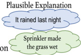
Abductive reasoning (AR) is inference to the best explanation. It typically starts from an incomplete set of observations about everyday situations and comes up with what can be considered the most likely possible explanation given these observations (Pople, 1973; Douven, 2017). One of the key characteristics that make abductive reasoning more challenging and distinct from other types of reasoning is its non-monotonic character (Strasser and Antonelli, 2019) i.e., even the most likely explanations are not necessarily correct. For example, in Figure 1, the most likely explanation for Observation 1: 'wet grass outside my house' is that 'it has been
Anette Frank
Research Training Group AIPHES Institute for Computational Linguistics Heidelberg University frank@cl.uni-heidelberg.de
Observation 1 :
The grass outside my house is wet
Observation 2 :
The sprinkler outside was switched on
Figure 1: Motivational example illustrating Abductive Reasoning and its non-monotonic character.
<details>
<summary>Image 1 Details</summary>
### Visual Description
## Diagram: Plausible Explanation
### Overview
The image is a simple diagram illustrating two **plausible explanations** for a phenomenon (e.g., wet grass). It uses two cloud-shaped elements to represent alternative hypotheses, with distinct colors and labels.
### Components/Axes
- **Title**: "Plausible Explanation" (top of the diagram).
- **Cloud 1 (Top)**:
- Color: Blue.
- Label: "It rained last night."
- **Cloud 2 (Bottom)**:
- Color: Green.
- Label: "Sprinkler made the grass wet."
- **No axes, legends, or numerical data** are present.
### Detailed Analysis
- The diagram visually separates two hypotheses using spatial positioning (top vs. bottom) and color differentiation (blue vs. green).
- No quantitative data, trends, or relationships between the elements are depicted.
- Text is explicitly embedded in the cloud shapes, with no additional annotations or contextual clues.
### Key Observations
1. The two explanations are presented as mutually exclusive or competing hypotheses.
2. Color coding (blue for rain, green for sprinkler) may imply categorical distinctions (e.g., natural vs. artificial causes).
3. No evidence of causality, probability, or interdependence between the explanations is provided.
### Interpretation
The diagram serves as a conceptual tool to contrast two possible causes for an observed outcome (e.g., wet grass). By isolating the explanations into distinct visual elements, it encourages critical evaluation of which hypothesis is more likely based on additional evidence (e.g., weather reports, sprinkler schedules). The absence of connecting lines or shared attributes suggests the explanations are independent, though real-world scenarios might involve overlapping factors (e.g., rain and sprinklers occurring simultaneously).
**Note**: This diagram lacks empirical data, so no statistical or numerical conclusions can be drawn. It is purely illustrative of logical reasoning frameworks.
</details>
raining' . However, when a new piece of information (observation or evidence) becomes available, the explanation must possibly be retracted, showing the defeasible character of abduction . With the new observation ( 'the sprinkler was switched on ') the most plausible explanation changes to 'Sprinkler caused the grass to be wet' . Humans, in such situations, could induce or validate such abductive inferences by performing hypothetical reasoning (such as 'What would happen if the sprinkler was switched on?' ) to arrive at a plausible explanation for 'wet grass outside my house' .
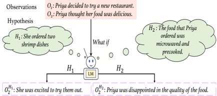
In this work, we focus on the α NLI task (Bhagavatula et al., 2020), where given two observations ( O 1 at time t 1 , O 2 at time t 2 , with t 1 < t 2 ) as an incomplete context, the task is to predict which of two given hypothesized events ( H 1 or H 2 ) is more plausible to have happened between O 1 and O 2 . Figure 2 illustrates this with an example: given observations O 1 :'Priya decided to try a new restaurant. ' and O 2 : 'Priya thought her food was delicious. ' , the task is to predict whether H 1 or H 2 is the more plausible explanation given observations O 1 and O 2 . Both H 1 and H 2 are different plausible hypothetical situations that can evolve from the same observation (premise) O 1 .
In this paper, we hypothesize that learning how different hypothetical scenarios ( H 1 and H 2 ) can result in different outcomes (e.g., O H j 2 , Fig. 2) can help in performing abductive inference. In order to decide which H i , is more plausible given observa-
Figure 2: Motivational example for α NLI : The top box (red) shows the observations and two callout clouds (green) contain the hypotheses. The implications ( O H i i ) - generated by the LM conditioned on each hypothesis and the observations - are given in pink colored boxes.
<details>
<summary>Image 2 Details</summary>
### Visual Description
## Diagram: Priya's Restaurant Experience Hypothesis Testing
### Overview
The diagram illustrates a logical reasoning process where observations about Priya's restaurant experience lead to two competing hypotheses (H₁ and H₂), each generating distinct outcomes (O^H₁ and O^H₂). A central "LM" (likely representing a logical model or decision node) connects the hypotheses to their outcomes.
### Components/Axes
- **Observations (Top)**:
- O₁: "Priya decided to try a new restaurant."
- O₂: "Priya thought her food was delicious."
- **Hypotheses (Middle)**:
- H₁: "She ordered two shrimp dishes."
- H₂: "The food that Priya ordered was microwaved and precooked."
- **Outcomes (Bottom)**:
- O^H₁: "She was excited to try them out."
- O^H₂: "Priya was disappointed in the quality of the food."
- **Central Node**:
- "LM" (Logical Model/Decision Node) with a question mark, linking hypotheses to outcomes.
### Detailed Analysis
- **Flow**:
Observations (O₁, O₂) → Hypotheses (H₁, H₂) → Outcomes (O^H₁, O^H₂).
Arrows indicate causal reasoning: hypotheses are derived from observations and lead to specific outcomes.
- **Textual Elements**:
All labels are in English. No non-English text is present.
### Key Observations
1. **Hypothesis Outcomes**:
- H₁ (shrimp dishes) → Positive outcome (excitement).
- H₂ (microwaved/precooked food) → Negative outcome (disappointment).
2. **Ambiguity in Observations**:
- O₂ ("food was delicious") conflicts with H₂'s negative outcome, suggesting H₂ may not align with Priya's actual experience.
3. **Central Node Role**:
- "LM" acts as a decision point, evaluating which hypothesis better explains the observations.
### Interpretation
The diagram models a **Peircean abductive reasoning process**:
- **Observations** (O₁, O₂) are facts to be explained.
- **Hypotheses** (H₁, H₂) are competing explanations.
- **Outcomes** (O^H₁, O^H₂) are predictions derived from each hypothesis.
**Key Insight**:
The conflict between O₂ ("delicious food") and H₂'s negative outcome (disappointment) implies H₂ may be less plausible. This suggests Priya's positive experience (O₂) is better explained by H₁ (enjoying shrimp dishes) rather than H₂ (poor food quality). The "LM" node highlights the need to test hypotheses against real-world outcomes to resolve ambiguity.
**Notable Pattern**:
The diagram emphasizes how subjective experiences (e.g., "delicious food") can be explained by multiple hypotheses, requiring further evidence to validate the most accurate explanation.
</details>
tions, we assume each H i to be true and generate a possible next event O H i 2 for each of them independently (e.g.: What will happen if Priya's ordered food was microwaved and precooked? ). We then compare the generated sentences ( O H 1 2 , O H 2 2 in Fig. 2) to what has been observed ( O 2 ) and choose as most plausible hypothesis the one whose implication is closest to observation O 2 .
We design a language model ( LM I ) which, given observations and a hypothesis, generates a possible event that could happen next, given one hypothesis. In order to train this language model, we use the TIMETRAVEL (TT) corpus (Qin et al., 2019) (a subpart of the ROCStories corpus 1 ). We utilize the LM I model to generate a possible next event for each hypothesis, given the observations. We then propose a multi-task learning model MTL that jointly chooses from the generated possible next events ( O H 1 2 or O H 2 2 ) the one most similar to the observation O 2 and predicts the most plausible hypothesis ( H 1 or H 2 ).
Our contributions are: i) To our best knowledge, we are the first to demonstrate that a model that learns to perform hypothetical reasoning can support and improve abductive tasks such as α NLI. We show that ii) for α NLI our multi-task model outperforms a strong BERT baseline (Bhagavatula et al., 2020).
Our code is made publicly available. 2
## 2 Learning about Counterfactual Scenarios
The main idea is to learn to generate assumptions, in a given situation, about 'What could have hap-
1 We ensure that α NLI testing instances are held out.
2 https://github.com/Heidelberg-NLP/ HYPEVENTS
<details>
<summary>Image 3 Details</summary>
### Visual Description
## Diagram: Sequential and Counterfactual Reasoning Models
### Overview
The image presents three interconnected diagrams (a, b, c) illustrating hypothetical reasoning processes involving observations (O), hypotheses (H), and states (S). Arrows represent causal or inferential relationships, with labels indicating specific reasoning mechanisms (e.g., "αNLI," "Counterfactual").
### Components/Axes
- **Nodes**:
- **Observations (O)**: Labeled as *O₁*, *O₂*, *O'₁*, *O'₂* (primed variants suggest counterfactual outcomes).
- **Hypotheses (H)**: Labeled as *H₁*, *H₂*, *Hᵢ* (subscript *i* implies variable indexing).
- **States (S)**: Labeled as *S₁*, *S₂*, *S₃*, *S'₂*, *S'₃* (primed variants denote altered states).
- **Arrows**:
- Solid arrows indicate direct causal/inferential links.
- Dashed arrows (e.g., in diagram b) represent counterfactual or hypothetical pathways.
- **Labels**:
- Diagram (a): "αNLI" (likely a reasoning method).
- Diagram (b): "Counterfactual" (explicitly labeled on a dashed arrow).
### Detailed Analysis
#### Diagram (a): αNLI
- **Flow**: *O₁* → *Hᵢ* → *O₂*.
- **Interpretation**: A standard inference chain where observation *O₁* leads to hypothesis *Hᵢ*, which in turn predicts observation *O₂*.
#### Diagram (b): Counterfactual Reasoning from TimeTravel
- **Flow**:
- *S₁* → *S₂* → *S₃* (primary causal path).
- *S₂* → *S'₃* (counterfactual path, dashed arrow).
- **Key Elements**:
- The counterfactual arrow from *S₂* to *S'₃* suggests exploring alternative outcomes if *S₂* were modified.
- *S'₂* and *S'₃* are primed states, indicating deviations from the original trajectory.
#### Diagram (c): Hypothesis Branching
- **Flow**:
- *O₁* branches to *H₁* and *H₂*.
- *H₁* → *O'₁*, *H₂* → *O'₂*.
- **Interpretation**: A bifurcated hypothesis space where *O₁* generates two hypotheses (*H₁*, *H₂*), each leading to distinct counterfactual outcomes (*O'₁*, *O'₂*).
### Key Observations
1. **Counterfactuality**: Diagrams (b) and (c) explicitly model alternative outcomes (*S'₃*, *O'₁*, *O'₂*), suggesting a focus on "what-if" scenarios.
2. **Hypothesis-Driven Inference**: All diagrams emphasize hypotheses (*Hᵢ*, *H₁*, *H₂*) as intermediaries between observations and outcomes.
3. **State Transitions**: Diagram (b) introduces state transitions (*S₁* → *S₂* → *S₃*), implying temporal or sequential reasoning.
### Interpretation
The diagrams collectively model a framework for **counterfactual reasoning** in natural language inference (NLI). Diagram (a) represents baseline inference, while (b) and (c) extend this to explore hypothetical scenarios. The use of primed states (*S'*, *O'*) and dashed arrows highlights deviations from observed reality, aligning with time-travel-inspired reasoning. This structure could underpin systems that evaluate the robustness of hypotheses under altered conditions, critical for tasks like anomaly detection or speculative analysis.
No numerical data or trends are present; the focus is on conceptual relationships and reasoning pathways.
</details>
(c) Learning to generate possible future event for each hypothesis
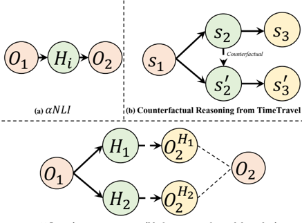
Figure 3: Different reasoning schemes and settings for our task and approach. The arrows denote the direction (temporal flow) of the reasoning chain. The dotted arrow in (b) denotes the derivation of a counterfactual situation s ′ 2 from a factual s 2 . In (c), the dotted arrows denote the learned inference; the dotted lines indicate the similarity between O 2 and O H i 2 .
pened (next) if we had done X?' or 'What could happen (next) if we do X?' (Bhatt and Flanagan, 2010). Figure 3(a) depicts the α NLI task framework. We hypothesize that getting to know what will happen (next) if any of two hypotheses occurs , will help us verifying which of them is more plausible (see Fig. 3(c)). Therefore, we encourage the model to learn how different hypothetical events (including counterfactual events) evolving from the same premise ( s 1 ) can lead to different or similar outcomes (see Fig. 3(b)).
Accordingly, we teach a pre-trained GPT-2 (Radford et al., 2019) language model how to generate a sequence of possible subsequent events given different hypothetical situations in a narrative setting. Training such a model on narrative texts encourages it to learn causal and temporal relations between events. We train a conditional language model, LM I , which generates a possible event that could happen next, given some counterfactual scenarios for a given story.
We train this model on the TIMETRAVEL (TT) dataset (Qin et al., 2019), by fine-tuning GPT-2 to learn about possible next events emerging from a situation in a story, given some alternative, counterfactual event. The TT dataset consists of fivesentence instances S =( s 1 , s 2 ,.., s 5 ) 3 from the ROCStories corpus 1 plus additional crowd-sourced sen-
3 s 1 = premise , s 2 = initial context , s 3:5 = original ending
O
1 : Dotty was being very grumpy. 2 : She felt much better afterwards. 1 : Dotty ate something bad. 2 Dotty call some close friends to chat. H 2 : She started to feel sick. : They all tried to make her happy.
O
H
H :
O 1
O H 2 2
Table 1: Example of generated possible next events O H j 2 using the LM I model. Bold hypothesis ( H 2 ) is more plausible.
tences s ′ 2:5 , where s ′ 2 is counterfactual 4 to s 2 from the original story 5 . There are two reasons for using the TT dataset for our purposes: a) the domains on which GPT-2 was pretrained are broad 6 and different from the domain of ROCStories, b) the model can see how alternative situations can occur starting from the same premise s 1 , resulting in similar or different outcomes. Note that, although intermediate situations may be counterfactual to each other, the future outcome can still be similar to the original ending due to causal invariance 7 .
Concretely, the language model LM I reads the premise ( s 1 ) and the alternative event(s) ( s 2 or s ′ 2 ), the masked token (serving as a placeholder for the missing possible next event(s) ( s 3: i or s ′ 3: i ), then the rest of the story ( s i +1:5 or s ′ i +1:5 ) and again the premise ( s 1 ). We train the model to maximize the log-likelihood of the missing ground-truth sentence(s) ( s 3: i ).
$$\mathcal { L } ^ { L M _ { \mathcal { I } } } ( \beta ) = \begin{array} { r l } & { t h e o u n d B E R T a t e o u n d e v e n s h o u l } \\ \log _ { p _ { \beta } } ( s _ { 3 ; i } | [ S ] s _ { 1 } , [ M ] , s _ { i + 1 ; 5 } , [ E ] , [ S ] , s _ { 1 } , s _ { 2 } ) & ( 1 ) } \end{array}$$
where i ∈ [3 , 4] , s i = { w s i 1 , .., w s i n } a sequence of tokens, [ S ] =start-of-sentence token, [ E ] =end-ofsentence token, [ M ] =mask token.
## 3 Generating Hypothetical Events to support the α NLI task
In this paper, we aim to investigate whether models perform better on the α NLI task when explicitly learning about events that could follow other events in a hypothetical scenario. We do so by introducing two methods LM I + BERTScore and LM I +
4 a counterfactual s ′ states something that is contrary to s
During our experiments we treat them as two separate S s S s s ′
5 instances: 1 =( 1:5 ) and 2 = ( 1 , 2:5 ).
6 GPT-2 was trained on the WebText Corpus.
7 the future events that are invariant under the counterfactual conditions (Qin et al., 2019)
MTL for unsupervised and supervised settings, respectively.
We first apply the trained model LM I on the α NLI task, where the given observations O 1 and O 2 , and alternative hypotheses H j are fed as shown in (2) below. 8
$$\begin{array} { r l } { v e n t s } & O _ { 2 } ^ { H _ { j } } = \beta ( [ S ] , O _ { 1 } , [ M ] , O _ { 2 } , [ E ] , [ S ] , O _ { 1 } , H _ { j } ) \quad ( 2 ) } \end{array}$$
We generate a possible next event for each hypothetical event H j , i.e., O H 1 2 and O H 2 2 (or: what will happen if some hypothesis H j occurs given the observations), where j ∈ [1 , 2] . Table 1 illustrates an example where different O H j 2 are generated using LM I . One of the challenges when generating subsequent events given a hypothetical situation is that there can be infinite numbers of possible next events. Therefore, to constrain this range, we chose to give future events ( O 2 ) as input, such that the model can generate subsequent events in a constrained context.
## 3.1 Unsupervised Setting
In this setting, we do not train any supervised model to explicitly predict which hypothesis is more plausible given the observations. Instead, we apply the fine-tuned LM I model to the α NLI data, generate possible next events O H j 2 given O 1 and H j , as described above, and measure the similarity between such possible next events ( O H j 2 ) and the observation ( O 2 ) in an unsupervised way, using BERTScore (BS) (Zhang et al., 2020) 9 . We evaluate our hypothesis that the generated possible next event O H j 2 given the more plausible hypothesis H j should be more similar to observation O 2 . Table 1 illustrates an example where H 2 is the more plausible hypothesis. We impose the constraint that for a correctly predicted instance BS( O 2 H + , O 2 ) > BS( O 2 H -, O 2 ) should hold, where H + , H -are the more plausible vs. implausible hypothesis, respectively.
## 3.2 Supervised Setting
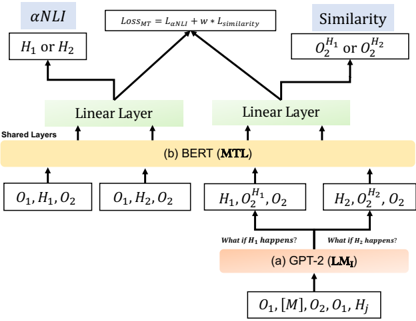
In this setting, displayed in Figure 4, we explore the benefits of training a multi-task MTL model that predicts i) the most plausible hypothesis and ii) which possible next event ( O H j 2 ) is more similar
8 For definition of placeholders see (1).
9 BERTScore is an automatic evaluation metric for text generation that leverages the pre-trained contextual embeddings from BERT and matches words in candidate and reference sentences by cosine similarity.
Figure 4: Overview of our LM I + MTL model for α NLI: (a) language model LM I takes the input in a particular format to generate different possible next events, (b) the MTL model learns to predict the best explanation ( H j ) and possible next events ( O H j 2 ) at the same time to perform the α NLI task.
<details>
<summary>Image 4 Details</summary>
### Visual Description
## Diagram: Machine Learning Model Architecture Comparison (GPT-2 vs BERT with Custom Components)
### Overview
The diagram illustrates a hybrid machine learning architecture combining elements of GPT-2 (LM₁) and BERT (MTL) models, with additional components for αNLI (Adversarial Natural Language Inference), similarity scoring, and multi-task learning (MTL). The architecture includes shared layers, linear layers, hypothesis-specific outputs, and a composite loss function.
### Components/Axes
1. **Core Components**:
- **Shared Layers**: Central processing unit for both GPT-2 and BERT variants
- **Linear Layers**: Two separate linear transformation modules (one per model variant)
- **αNLI**: Adversarial Natural Language Inference component
- **Similarity**: Similarity scoring mechanism
- **Loss_MT**: Composite loss function (L_αNLI + w * L_similarity)
2. **Input/Output Flows**:
- **Inputs**: O₁, H₁, O₂ (base outputs)
- **Hypothesis Variants**: H₁ or H₂ (conditional processing paths)
- **Output Variants**:
- GPT-2 (LM₁): O₁, [M], O₂, O₁, H_j
- BERT (MTL): H₁, O₂¹, O₂; H₂, O₂², O₂
3. **Key Elements**:
- **Conditional Processing**: "What if H₁ happens?" and "What if H₂ happens?" decision nodes
- **Output Modifiers**: O₂¹/O₂² (hypothesis-specific output versions)
- **Loss Function**: Weighted combination of αNLI loss and similarity loss
### Detailed Analysis
1. **Shared Layers**:
- Process base inputs (O₁, H₁, O₂) for both model variants
- Serve as foundation for both GPT-2 and BERT implementations
2. **Linear Layers**:
- Two distinct linear transformation modules
- One for GPT-2 (LM₁) path
- One for BERT (MTL) path
3. **αNLI Component**:
- Takes H₁ or H₂ as input
- Feeds into Loss_MT calculation
4. **Similarity Scoring**:
- Processes O₂¹ or O₂²
- Contributes to Loss_MT via weighted term (w * L_similarity)
5. **Hypothesis-Specific Paths**:
- **H₁ Path**:
- Input: H₁
- Output: O₂¹, O₂
- **H₂ Path**:
- Input: H₂
- Output: O₂², O₂
6. **Output Variants**:
- **GPT-2 (LM₁)**: Maintains original output structure with additional hypothesis component (H_j)
- **BERT (MTL)**: Produces hypothesis-specific output versions (O₂¹/O₂²) while maintaining base output (O₂)
### Key Observations
1. **Architectural Integration**:
- Shared layers enable parameter efficiency
- Linear layers provide model-specific adaptations
2. **Multi-Task Capabilities**:
- αNLI component adds adversarial training dimension
- Similarity scoring enables cross-output consistency
3. **Conditional Processing**:
- Model behavior adapts based on hypothesis (H₁/H₂)
- Different output configurations for each hypothesis path
4. **Loss Function Design**:
- Balances adversarial training (L_αNLI) with output consistency (L_similarity)
- Weight parameter (w) controls similarity loss contribution
### Interpretation
This architecture demonstrates a sophisticated approach to multi-task learning in NLP:
1. **Efficiency Through Sharing**: Shared layers reduce parameter count while maintaining model flexibility
2. **Adversarial Robustness**: αNLI component suggests focus on handling challenging linguistic cases
3. **Hypothesis-Aware Processing**: The model can adapt its output based on different linguistic hypotheses
4. **Composite Training Objective**: The loss function balances multiple objectives, suggesting a focus on both adversarial performance and output consistency
The diagram reveals a hybrid approach that combines the strengths of transformer-based models (GPT-2's generative capabilities and BERT's bidirectional understanding) with custom components for specific NLP tasks. The conditional processing paths indicate the model's ability to handle different linguistic scenarios, while the shared architecture components suggest efficient parameter utilization.
</details>
to the observation ( O 2 ). Multi-task learning aims to improve the performance of a model for a task by utilizing the knowledge acquired by learning related tasks (Ruder, 2019). We hypothesize that a) the possible next event O H j 2 of the more plausible hypothesis H j should be most similar to observation O 2 , and that b) learning which possible next event is more similar supports the model in the α NLI task ( inductive transfer ).
The architecture of LM I + MTL model is shown in Figure 4. The model marked (a) in Figure 4 depicts the LM I model as described in §3. The outputs of the LM I model, which we get from Eq. (2) for both hypotheses are incorporated as an input to the MTL model. Concretely, we feed the MTL classifier a sequence of tokens as stated in part (b) of Figure 4, and aim to compute their contextualized representations using pre-trained BERT. The input format is described in Table 3. Similar to (Devlin et al., 2019), two additional tokens are added [CLS] at the start of each sequence input and [SEP] at the end of each sentence. In the shared layers (see Fig 4(b)), the model first transform the input sequence to a sequence of embedding vectors. Then it applies an attention mechanism that learns contextual relations between words (or sub-words) in the input sequence.
For each instance we get four [CLS] embeddings ( CLS H j , CLS O Hj 2 ; j ∈ [1 , 2] ) which are then passed through two linear layers, one for the α NLI (main task) and another for predicting the
Table 2: Dataset Statistics: nb. of instances
| Task | Train | Dev | Test |
|------------------|---------|-------|--------|
| α NLI | 169654 | 1532 | 3059 |
| TimeTravel (NLG) | 53806 | 2998 | - |
Table 3: Input and output format for the α NLI task: [CLS] is a special token used for classification, [SEP] a delimiter.
| Input Format | Output |
|-----------------------------------------|--------------------|
| [CLS] O 1 [SEP] H i [SEP] O 2 [SEP] | H 1 or H 2 |
| [CLS] H i [SEP] O H i 2 [SEP] O 2 [SEP] | O H 1 2 or O H 2 2 |
similarity (auxiliary task) between O H j 2 and O 2 . We compute the joint loss function L = L αNLI + w ∗ L similarity ; where w is a trainable parameter, L αNLI and L similarity are the loss function for the αNLI task and auxiliary task, respectively.
## 4 Experimental Setup
Data. We conduct experiments on the ART (Bhagavatula et al., 2020) dataset. Data statistics are given in Table 2. For evaluation, we measure accuracy for α NLI.
Hyperparameters. To train the LM I model we use learning rate of 5 e -05 . We decay the learning rate linearly until the end of training; batch size: 12. In the supervised setting for the α NLI task , we use the following set of hyperparameters for our MTL model with integrated LM I model ( LM I + MTL ): batch size: { 8 , 16 } ; epochs: { 3 , 5 } ; learning rate: { 2 e -5 , 5 e -6 } . For evaluation, we measure accuracy. We use Adam Optimizer, and dropout rate = 0 . 1 . We experimented on GPU size of 11 GB and 24 GB. Training is performed using cross-entropy loss. The loss function is L αNLI + w ∗ L similarity , where w is a trainable parameter. During our experiment we initialize w = 1 . The input format is depicted in Table 3. We report performance by averaging results along with the variance obtained for 5 different seeds.
Baselines. We compare to the following baseline models that we apply to the α NLI task, training them on the training portion of the ART dataset (cf. Table 2).
- ESIM + ELMo is based on the ESIM model previously used for NLI (Chen et al., 2017). We use (a) ELMo to encode the observations and hypothesis, followed by (b) an attention
Table 4: Results on α NLI task , : as in Bhagavatula et al. (2020) (no unpublished leaderboard results). For each row, the best results are in bold, and performance of our models are in blue.
| Model | Dev Acc.(%) Test Acc.(%) | Dev Acc.(%) Test Acc.(%) |
|----------------------------------------------|----------------------------|----------------------------|
| Majority ( from dev set ) | - | 50.8 |
| LM I + BERTScore | 62.27 | 60.08 |
| Infersent | 50.9 | 50.8 |
| ESIM + ELMo | 58.2 | 58.8 |
| BERT Large | 69.1 | 68.9 ± 0 . 5 |
| GPT-2 + MTL | 68.9 ± 0 . 3 | 68.8 ± 0 . 3 |
| COMET + MTL | 69.4 ± 0 . 4 | 69.1 ± 0 . 5 |
| LM I + MTL | 72.9 ± 0 . 5 | 72.2 ± 0 . 6 |
| Human Performance | - | 91.4 |
layer, (c) a local inference layer, and (d) another bi-directional LSTM inference composition layer, and (e) a pooling operation,
- Infersent (Conneau et al., 2017) uses sentence encoding based on a bi-directional LSTM architecture with max pooling.
- BERT (Devlin et al., 2019) is a LM trained with a masked-language modeling (MLM) and next sentence prediction objective.
As baselines for using the MTL model, we replace LM I with alternative generative LMs:
- GPT-2 + MTL . In this setup, we directly use the pretrained GPT-2 model and task it to generate a next sentence conditioned on each hypothesis ( O H i 2 ) without finetuning it on the TIMETRAVEL data. We then use the supervised MTL model to predict the most plausible hypothesis and which of the generated observations is more similar to O 2 .
- COMET + MTL . In this setting, we make use of inferential if-then knowledge from ATOMIC (Sap et al., 2019a) as background knowledge. Specifically, we use COMET to generate objects with Effect 10 relations for each hypothesis as a textual phrase.
## 5 Results
In Table 4, we compare our models LM I + BERTScore and LM I + MTL against the models proposed in Bhagavatula et al. (2020): a majority baseline, supervised models ( Infersent and
10 as a result PersonX feels; as a result PersonX wants; PersonX then
ESIM+ELMo ), as well as BERT Large . Bhagavatula et al. (2020) re-train the ESIM+ELMo and Infersent models on the ART dataset and fine-tuned the BERT model on the α NLI task and report the results.
We find that our unsupervised model with BERTScore ( LM I + BERTScore) outperforms (by +9 . 28 pp. and +1 . 28 pp.) strong ESIM+ELMo and Infersent baseline models. Table 5 shows some examples of our generation model LM I along with the obtained BERTScores.
Unlike the unsupervised LM I + BERTScore, our supervised LM I + MTL model also improves over the BERT Large baseline, by +3 . 3 pp. We can attribute the improvement to the model having been jointly trained to assess the similarity and dissimilarity of possible next events O H j 2 and observations ( O 2 ) along with the α NLI task. One of the advantages of training our proposed multitask learning ( MTL ) model, instead of directly feeding the possible next events O H j 2 as knowledge inputs is that it adds an explainable component to the model. One can view the generated next events O H j 2 as natural language rationales and our multitask model explicitly chooses one of them. Hence, the multi-task framework makes the model more expressive. Finally, we compare, for the MTL model, our embedded generation model LM I to pre-trained GPT-2 and COMET. Table 4 shows that LM I + MTL yields better performance compared to both COMET + MTL ( +3 . 1 pp.) and GPT-2 + MTL ( +3 . 4 pp.) - the intuitive reason being that the next events generated by LM I are more helpful than events generated using pretrained GPT-2 and objects generated by COMET.
Table 5 illustrates some examples where our MTL model not only chooses the correct hypothesis, but also a likely possible next event that is similar to the observation O 2 . Interestingly, during training of MTL we initialize w = 1, and after training the model we found the w value had been adjusted to a range between 0 . 85 and 0 . 75 , which intuitively shows both the effectiveness of our LM I -generated possible next events, and their similarity to the given observations O 2 .
## 5.1 Case Study
Table 5 displays possible next events, generated by our LM I model - along with the BERTscore measured between the possible next events O H j 2 and observation O 2 . We see two different scenarios:
Table 5: Examples of generated possible next events for solving α NLI using our LM I model. Column 3: Hypothesis and possible next events chosen by our LM I + MTL model; Column 4: Reasoning type between the hypothesis H j and O 2 ; Column 5: BERTScore between the O H j 2 and O 2 ; Column5: Human evaluation of the possible next events with respect the observation O 2 .
| Observation ( O ) | Given Hypotheses ( H j ) | What if H j happens? Generated possible next events O H j 2 | MTL | Reasoning Type | BERT Score | Human Evalua- tion |
|-------------------------------------------------------------------|--------------------------------------------------------------------|---------------------------------------------------------------------|---------------|------------------|--------------|----------------------|
| a. O 1 : Jim got ready for his first date. | H 1 : Jim's date wasn't at- tracted to him. | O H 2 1 : He tried to get her num- ber. She never responded to him. | H 1 , O H 1 2 | Reaction | 47.34 | Non- Contradiction |
| O 2 : Since then, she has ig- nored all of Jim's text mes- sages. | H 2 : Jim went on the date and said he didn't like the girl. | O H 2 2 : He told her that he didn't want to date her. | | | 44.19 | Contradiction |
| b. O 1 : Nate had the summer off before college. | H 1 : Nate spent the summer traveling and partying. | O H 1 2 : Nate had a lot of fun. | H 1 , O H 1 2 | Motivation | 49.02 | Non- Contradiction |
| O 2 : Nate's last summer before college was a total blast! | H 2 :Nate decided to spend the entire summer working in the Mines. | O H 2 2 : Nate spent the summer working in the mines. | | | 44.34 | Redundancy |
| c. O 1 : Dotty was being very grumpy. | H 1 : Dotty ate something bad. | O H 1 2 : She started to feel sick. | H 2 , O H 2 2 | Emotional Effect | 0.604 | Contradiction |
| O 2 : She felt much better afterwards | H 2 : Dotty call some close friends to chat. | O H 2 2 : They all tried to make her happy. | | | 0.405 | Non- Contradiction |
| d. O 1 : Cay had a crush on a boy in her class. | H 1 : Cay sent a love note to the boy. | O H 1 2 : The boy responded and said he liked Cay. | H 1 , O H 1 2 | Emotional Effect | 0.509 | Non- Contradiction |
| O 2 : He smiled at her after and said he liked her too! | H 2 : She told him she did not like him. | O H 2 2 : The boy was very sad about it. | | | 0.423 | Contradiction |
(i) examples (a), (b) and (d) depicting the scenario where possible next events and observation pairs correctly achieve higher BERTscores 11 , (ii) example (c) depicting the scenario where an incorrect possible next event and observation pair achieves higher BERTscores than the correct one. Intuitive reasons for these scenarios are, for example, for (a): there is a higher word overlap and semantic similarity between a correct next event and observation O 2 , for example (b): there is higher semantic similarity; whereas for example (c): although there is a higher semantic dissimilarity, the word overlap between the wrong possible next event ( 'She started to feel sick. ' ) and the observation ( 'She felt much better afterwards. ' ) is much higher.
## 6 Manual Evaluation
Since the automatic scores only account for wordlevel similarity between observations and generated possible next events, we conduct a manual evaluation study, to assess the quality of sentences generated by our LM I model.
Annotation Study on LM I generations. The annotation was performed by three annotators with computational linguistic background. We provide each of the three annotators with observations, hypotheses and sentences, as produced by our LM I
11 BERTscore matches words in candidate and reference sentences by cosine similarity.
model, for 50 randomly chosen instances from the α NLI task. They obtain i) generated sentences for a next possible event for the correct and incorrect hypothesis , as well as ii) the sentence stating observation O 2 .
We ask each annotator to rate the sentences according to four quality aspects as stated below.
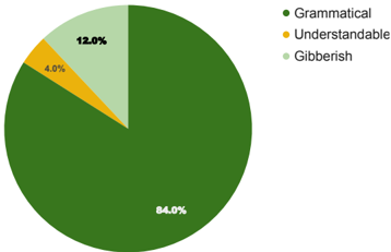
Grammaticality: the sentence is i) grammatical, ii) not entirely grammatical but understandable, or iii) completely not understandable;
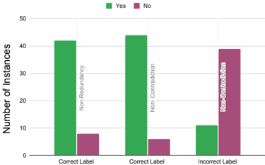
Redundancy: the sentence contains redundant or repeated information;
Contradiction: the sentence contains any pieces of information that are contradicting the given observation O 2 or not;
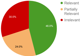
Relevance: the possible next event is i) relevant, ii) partially relevant, or iii) not relevant.
For each aspect, they are asked to judge the sentence generated for the correct hypothesis 12 . Only for Contradiction , they are asked to judge both sentences, for correct and the incorrect hypotheses.
Results and Discussion. Figures 5, 7, and 6 present the results of manual evaluations of the generation quality, according to the different criteria described above.
12 The correct hypothesis was marked for the annotation.
Figure 5: Human evaluation of the grammaticality of generated sentences: ratio of i) grammatical, ii) not entirely grammatical but understandable, iii) completely not understandable sentences.
<details>
<summary>Image 5 Details</summary>
### Visual Description
## Pie Chart: Distribution of Text Categories
### Overview
The image displays a pie chart illustrating the distribution of three text categories: Grammatical, Understandable, and Gibberish. The chart uses distinct colors for each category, with percentages labeled directly on the slices. The legend is positioned to the right of the chart for reference.
### Components/Axes
- **Legend**: Located on the right side of the chart, with three entries:
- **Dark Green**: Grammatical (84.0%)
- **Yellow**: Understandable (4.0%)
- **Light Green**: Gibberish (12.0%)
- **Chart Segments**: Three proportional slices representing the categories, with percentages annotated on each slice.
### Detailed Analysis
1. **Grammatical (84.0%)**:
- Color: Dark Green
- Position: Dominates the majority of the pie chart, occupying 84% of the total area.
- Annotation: "84.0%" is clearly marked in white text on the dark green segment.
2. **Understandable (4.0%)**:
- Color: Yellow
- Position: Smallest slice, occupying 4% of the chart.
- Annotation: "4.0%" is marked in white text on the yellow segment.
3. **Gibberish (12.0%)**:
- Color: Light Green
- Position: Second-largest slice, occupying 12% of the chart.
- Annotation: "12.0%" is marked in white text on the light green segment.
### Key Observations
- The **Grammatical** category overwhelmingly dominates the distribution, accounting for 84% of the total.
- The **Understandable** category is the smallest, representing only 4% of the data.
- The **Gibberish** category, while significantly smaller than Grammatical, is 3 times larger than Understandable (12% vs. 4%).
### Interpretation
The data suggests a strong emphasis on **Grammatical** text, which constitutes the vast majority of the analyzed content. The near-absence of **Understandable** text (4%) raises questions about the criteria used to classify text as "understandable" versus "gibberish." The **Gibberish** category (12%) may represent text that is syntactically correct but semantically nonsensical, highlighting a potential gap in the classification system. The stark contrast between Grammatical and Understandable categories could indicate a need for further refinement in text analysis methodologies to better capture nuanced distinctions between meaningful and nonsensical content.
</details>
Figure 6: Human evaluation of the Relevance of generated sentences for possible next events.
<details>
<summary>Image 6 Details</summary>
### Visual Description
## Pie Chart: Data Relevance Distribution
### Overview
The image displays a pie chart illustrating the distribution of data relevance across three categories: "Relevant," "Partially Relevant," and "Irrelevant." The chart uses distinct colors to differentiate categories, with a legend positioned to the right of the chart.
### Components/Axes
- **Legend**: Located on the right side of the chart, with three entries:
- Green circle labeled "Relevant"
- Orange circle labeled "Partially Relevant"
- Red circle labeled "Irrelevant"
- **Segments**:
- Green segment (46.0%) occupying the largest portion of the chart.
- Orange segment (24.0%) positioned adjacent to the green segment.
- Red segment (30.0%) completing the chart, adjacent to both green and orange segments.
### Detailed Analysis
- **Relevant (Green)**: 46.0% of the data is classified as fully relevant. This segment is the largest, occupying slightly less than half of the pie chart.
- **Partially Relevant (Orange)**: 24.0% of the data falls into this category, represented by the second-largest segment.
- **Irrelevant (Red)**: 30.0% of the data is marked as irrelevant, forming the third segment. This is larger than the "Partially Relevant" category but smaller than "Relevant."
### Key Observations
1. **Dominance of Relevant Data**: The "Relevant" category constitutes nearly half of the dataset, indicating a majority of items meet full relevance criteria.
2. **Irrelevant Data Proportion**: The "Irrelevant" category (30.0%) is notably larger than "Partially Relevant" (24.0%), suggesting a significant portion of data lacks relevance.
3. **Color Consistency**: All segments align with their corresponding legend labels (green = relevant, orange = partially relevant, red = irrelevant).
### Interpretation
The data suggests a dataset where relevance is unevenly distributed. While the majority of items are fully relevant, a substantial minority (30%) are entirely irrelevant, outnumbering the "Partially Relevant" group. This could imply challenges in data quality or filtering processes. The "Partially Relevant" category, though smaller than "Irrelevant," may represent items requiring further refinement or contextual analysis. The chart highlights the need for targeted improvements in data curation to reduce irrelevance while leveraging the dominant relevant portion effectively.
</details>
For measuring inter-annotator agreement, we computed Krippendorff's α (Hayes and Krippendorff, 2007) for Grammaticality and Relevance , as it is suited for ordinal values, and Cohen's Kappa κ for Redundancy and Contradiction . We found α values are 0 . 587 and 0 . 462 for Grammaticality and Relevance , respectively (moderate agreement) and κ values 0 . 61 and 0 . 74 for Redundancy and Contradiction (substantial agreement). We aggregated the annotations from the three annotators using majority vote. Figure 5 shows that the majority of sentences ( 96 %) are grammatical or understandable. Figure 7 shows that most sentences for correct labels are non-redundant ( 84 %) and noncontradictory ( 88 %), whereas for incorrect labels 39 instances are found to be contradictory with the observation O 2 ( 78 %). The manual evaluation supports our hypothesis that the generated sentences for correct labels should be more similar (less contradictory) compared to the sentences generated for incorrect labels. Figure 6 shows the ratio of sentences considered by humans as relevant, partially relevant, and irrelevant. The results show that 46 % of cases are relevant (based on majority agreement) and 24 %of cases are partially relevant. This yields that the generated sentences are (partially) relevant
Figure 7: Human evaluation of Redundancy and Contradiction of generations for possible next events.
<details>
<summary>Image 7 Details</summary>
### Visual Description
## Bar Chart: Label Validation Distribution
### Overview
The chart displays a comparative analysis of label validation results across three categories: "Correct Label (Non-Redundancy)", "Correct Label (Non-Contradiction)", and "Incorrect Label (Non-Contradiction)". Each category contains two bars representing "Yes" (green) and "No" (purple) responses, with counts on a y-axis scaled from 0 to 50.
### Components/Axes
- **X-Axis**: Three categories:
1. Correct Label (Non-Redundancy)
2. Correct Label (Non-Contradiction)
3. Incorrect Label (Non-Contradiction)
- **Y-Axis**: "Number of Instances" (0–50)
- **Legend**:
- Green = "Yes" (validated)
- Purple = "No" (invalidated)
- **Bar Placement**:
- "Yes" bars positioned left of each category
- "No" bars positioned right of each category
### Detailed Analysis
1. **Correct Label (Non-Redundancy)**:
- Yes: ~42 instances (green)
- No: ~8 instances (purple)
2. **Correct Label (Non-Contradiction)**:
- Yes: ~44 instances (green)
- No: ~6 instances (purple)
3. **Incorrect Label (Non-Contradiction)**:
- Yes: ~11 instances (green)
- No: ~39 instances (purple)
### Key Observations
- **High Agreement for Correct Labels**: Both "Non-Redundancy" and "Non-Contradiction" correct labels show >80% "Yes" validation (42/50 and 44/50 respectively).
- **Significant Disagreement for Incorrect Labels**: The "Incorrect Label" category has a near-inversion, with 39/50 "No" responses (78% invalidation).
- **Consistency in "No" Responses**: "No" counts are relatively low (~6–8) for correct labels but spike to ~39 for incorrect labels.
### Interpretation
The data suggests a strong consensus in validating correct labels for non-redundancy and non-contradiction, with >80% agreement. However, incorrect labels exhibit a starkly different pattern, where 78% of instances are flagged as contradictions. This implies that:
1. **Label Quality Matters**: Correct labels are robustly validated, while incorrect ones are heavily scrutinized.
2. **Contradiction Sensitivity**: The "Non-Contradiction" metric appears more sensitive to label errors than "Non-Redundancy".
3. **Potential System Bias**: The high "No" rate for incorrect labels may indicate an overzealous validation system or a dataset where contradictions are more prevalent in mislabeled instances.
The chart highlights the importance of precise labeling in maintaining data integrity, particularly for contradiction checks.
</details>
in most cases and thus should support abduction for both unsupervised ( LM I + BERTScore) and supervised ( LM I + MTL ) models.
Impact of Reasoning types. Finally, to better assess the performance of our model, we determine what types of reasoning underly the abductive reasoning tasks in our data, and examine to what extent our models capture or not these reasoning types. We consider again the 50 instances that were annotated by our previous annotators and manually classify them into different reasoning types. We broadly divided the data into 6 categories: (i) Motivation, (ii) Spatial-Temporal, (iii) Emotional, (iv) Negation, (v) Reaction, (vi) Situational fact. The most frequent type was Emotional (10), most infrequent was Spatial (7). We ask a new annotator to annotate the reasoning types for these 50 instances. Considering the relevance and contradiction categories from the previous annotations we determine that for Negation ( 8 ), Emotional ( 10 ), and Reaction ( 8 ) all generated events for correct labels are partially or fully relevant and non-contradictory . An intuitive reason can be that we train our LM I model to learn how different counterfactual hypothetical events emerging from a single premise can lead to the same or different outcomes through a series of events. Some counterfactual events ( s ′ 2 ) are negations of the original event ( s 2 ) in the TIMETRAVEL dataset. This may support the reasoning class Negation. For the other categories: Motivation, Spatial-temporal, and Situational fact, we detect errors regarding (missing) Relevance in 21 %, 14 %and 28 %of cases, respectively. Table 6 illustrates an example from the class Situational Fact, where our generated next event is irrelevant and redundant .
- O 1 : Jenna hit the weight hard in the gym.
O 2 : She took a cold bath in order to alleviate her pain.
- H 1 : Her neck pain stopped because of this.
H 2 : Jenna pulled a muscle lifting weights.
O 1 2 : She decided to take a break .
H
O H 2 2 : Jenna lost weight in the gym.
Table 6: Error Analysis: An example of generated possible next event O H j 2 from Situational Fact category.
## 7 Related Work
Commonsense Reasoning. There is growing interest in this research field, which led to the creation of several new resources on commonsense reasoning, in form of both datasets , such as SocialIQA (Sap et al., 2019b), CommonsenseQA (Talmor et al., 2019), CosmosQA (Huang et al., 2019) and knowledge bases , e.g. ConceptNet (Speer et al., 2017), ATOMIC (Sap et al., 2019a), or Event2Mind (Rashkin et al., 2018). Recently, many works proposed to utilize external static knowledge graphs (KGs) to address the bottleneck of obtaining relevant commonsense knowledge. Lin et al. (2019) proposed to utilize knowledge graph embeddings to rank and select relevant knowledge triples or paths. Paul and Frank (2019) proposed to extract subgraphs from KGs using graph-based ranking methods and further Paul et al. (2020) adopted the graph-based ranking method and proposed to dynamically extend the KG to combat sparsity. In concurrent work, Paul and Frank (2021) introduced a method to dynamically generate contextually relevant knowledge that guides a model while performing the narrative story completion task.
Both hypothetical reasoning and abductive reasoning are understudied problems in NLP. Recently, Tandon et al. (2019) proposed a first large-scale dataset of 'What if... ' questions over procedural text. They introduced the dataset to study the effect of perturbations in procedural text. Related to our work, Qin et al. (2019) investigated the capabilities of state-of-the-art LMs to rewrite stories with counterfactual reasoning. In our work we utilize this dataset to model how to generate possible next events emerging from different hypothetical and counterfactual events. Mostafazadeh et al. (2016) designed the narrative cloze task, a task to choose the correct ending of a story. 13 Conversely, Bhagavatula et al. (2020) proposed a task that requires
13 Their dataset, ROCStories, was later extended in Qin et al. (2019) and Bhagavatula et al. (2020).
reasoning about plausible explanations for narrative omissions. Our research touches on the issue of hypothetical reasoning about alternative situations. We found that making language models learn how different hypothetical events can evolve from a premise and result in similar or different future events forming from a premise and how these events can result in similar or different future events helps models to perform better in abduction.
Explainability. Despite the success of large pretrained language models, recent studies have raised some critical points such as: high accuracy scores do not necessarily reflect understanding (Min et al., 2019), large pretrained models may exploit superficial clues and annotation artifacts (Gururangan et al., 2018; Kavumba et al., 2019). Therefore, the ability of models to generate explanations has become desirable, as this enhances interpretability. Recently, there has been substantial effort to build datasets with natural language explanations (Camburu et al., 2018; Park et al., 2018; Thayaparan et al., 2020). There have also been numerous research works proposing models that are interpretable or explainable (Rajani et al., 2019; Atanasova et al., 2020; Latcinnik and Berant, 2020; Wiegreffe and Marasovi´ c, 2021). Our work sheds light in this direction, as our MTL model not only predicts the plausible hypothesis H j but also generates possible next events O H j 2 and chooses the one that is closer to the given context, thereby making our model more expressive.
Abductive Reasoning. There has been longstanding work on theories of abductive reasoning (Peirce, 1903, 1965a,b; Kuipers, 1992, 2013). Researchers have applied various frameworks, some focused on pure logical frameworks (Pople, 1973; Kakas et al., 1992), some on probabilistic frameworks (Pearl, 1988), and others on Markov Logics (Singla and Mooney, 2011). Recently, moving away from logic-based abductive reasoning, Bhagavatula et al. (2020) proposed to study languagebased abductive reasoning. They introduced two tasks: Abductive Natural Language Inference ( α NLI) and Generation ( α NLG) . They establish baseline performance based on state-of-the-art language models and make use of inferential structured knowledge from ATOMIC (Sap et al., 2019a) as background knowledge. Zhu et al. (2020) proposed to use a learning-to-rank framework to address the abductive reasoning task. Ji et al. (2020)
proposed a model GRF that enables pre-trained models (GPT-2) with dynamic multi-hop reasoning on multi-relational paths extracted from the external ConceptNet commonsense knowledge graph for the α NLG task. Paul and Frank (2020) have proposed a multi-head knowledge attention method to incorporate commonsense knowledge to tackle the α NLI task. Unlike our previous work in Paul and Frank (2020), which focused on leveraging structured knowledge, in this work, we focus on learning about what will happen next from different counterfactual situations in a story context through language model fine-tuning. Specifically, we study the impact of such forward inference on the α NLI task in a multi-task learning framework and show how it can improve performance over a strong BERT model.
## 8 Conclusion
We have introduced a novel method for addressing the abductive reasoning task by explicitly learning what events could follow other events in a hypothetical scenario, and learning to generate such events, conditioned on a premise or hypothesis. We show how a language model - fine-tuned for this capability on a suitable narrative dataset - can be leveraged to support abductive reasoning in the α NLI tasks, in two settings: an unsupervised setting in combination with BertScore , to select the proper hypothesis, and a supervised setting in a MTL setting.
The relatively strong performance of our proposed models demonstrates that learning to choose from generated hypothetical next events the one that is most similar to the observation, supports the prediction of the most plausible hypothesis. Our experiments show that our unsupervised LM I + BERTScore model outperforms some of the strong supervised baseline systems on α NLI. Our research thus offers new perspectives for training generative models in different ways for various complex reasoning tasks.
## Acknowledgements
This work has been supported by the German Research Foundation as part of the Research Training Group 'Adaptive Preparation of Information from Heterogeneous Sources' (AIPHES) under grant No. GRK 1994/1. We thank our annotators for their valuable annotations. We also thank NVIDIA Corporation for donating GPUs used in this research.
## References
Pepa Atanasova, Jakob Grue Simonsen, Christina Lioma, and Isabelle Augenstein. 2020. Generating fact checking explanations. In Proceedings of the 58th Annual Meeting of the Association for Computational Linguistics , pages 7352-7364, Online. Association for Computational Linguistics.
- Chandra Bhagavatula, Ronan Le Bras, Chaitanya Malaviya, Keisuke Sakaguchi, Ari Holtzman, Hannah Rashkin, Doug Downey, Wen tau Yih, and Yejin Choi. 2020. Abductive commonsense reasoning. In International Conference on Learning Representations .
- M. Bhatt and G. Flanagan. 2010. Spatio-temporal abduction for scenario and narrative completion ( a preliminary statement). In ECAI .
Oana-Maria Camburu, Tim Rockt¨ aschel, Thomas Lukasiewicz, and Phil Blunsom. 2018. e-SNLI: Natural Language Inference with Natural Language Explanations. In S. Bengio, H. Wallach, H. Larochelle, K. Grauman, N. Cesa-Bianchi, and R. Garnett, editors, Advances in Neural Information Processing Systems 31 , pages 9539-9549. Curran Associates, Inc.
Qian Chen, Xiaodan Zhu, Zhen-Hua Ling, Si Wei, Hui Jiang, and Diana Inkpen. 2017. Enhanced LSTM for natural language inference. In Proceedings of the 55th Annual Meeting of the Association for Computational Linguistics (Volume 1: Long Papers) , pages 1657-1668, Vancouver, Canada. Association for Computational Linguistics.
Alexis Conneau, Douwe Kiela, Holger Schwenk, Lo¨ ıc Barrault, and Antoine Bordes. 2017. Supervised learning of universal sentence representations from natural language inference data. In Proceedings of the 2017 Conference on Empirical Methods in Natural Language Processing , pages 670-680, Copenhagen, Denmark. Association for Computational Linguistics.
Jacob Devlin, Ming-Wei Chang, Kenton Lee, and Kristina Toutanova. 2019. BERT: Pre-training of deep bidirectional transformers for language understanding. In Proceedings of the 2019 Conference of the North American Chapter of the Association for Computational Linguistics: Human Language Technologies, Volume 1 (Long and Short Papers) , pages 4171-4186, Minneapolis, Minnesota. Association for Computational Linguistics.
Igor Douven. 2017. Abduction. In Edward N. Zalta, editor, The Stanford Encyclopedia of Philosophy , summer 2017 edition. Metaphysics Research Lab, Stanford University.
Suchin Gururangan, Swabha Swayamdipta, Omer Levy, Roy Schwartz, Samuel Bowman, and Noah A Smith. 2018. Annotation artifacts in natural language inference data. In Proceedings of the 2018 Conference of the North American Chapter of the
- Association for Computational Linguistics: Human Language Technologies, Volume 2 (Short Papers) , pages 107-112.
- A. Hayes and K. Krippendorff. 2007. Answering the call for a standard reliability measure for coding data. Communication Methods and Measures , 1:77 - 89.
- Lifu Huang, Ronan Le Bras, Chandra Bhagavatula, and Yejin Choi. 2019. Cosmos QA: Machine reading comprehension with contextual commonsense reasoning. In Proceedings of the 2019 Conference on Empirical Methods in Natural Language Processing and the 9th International Joint Conference on Natural Language Processing (EMNLP-IJCNLP) , pages 2391-2401, Hong Kong, China. Association for Computational Linguistics.
- Haozhe Ji, Pei Ke, Shaohan Huang, Furu Wei, Xiaoyan Zhu, and Minlie Huang. 2020. Language generation with multi-hop reasoning on commonsense knowledge graph. In Proceedings of the 2020 Conference on Empirical Methods in Natural Language Processing (EMNLP) , pages 725-736, Online. Association for Computational Linguistics.
- Antonis C Kakas, Robert A. Kowalski, and Francesca Toni. 1992. Abductive logic programming. Journal of logic and computation , 2(6):719-770.
- Pride Kavumba, Naoya Inoue, Benjamin Heinzerling, Keshav Singh, Paul Reisert, and Kentaro Inui. 2019. When Choosing Plausible Alternatives, Clever Hans can be Clever. In Proceedings of the First Workshop on Commonsense Inference in Natural Language Processing , pages 33-42, Hong Kong, China. Association for Computational Linguistics.
- Theo AF Kuipers. 1992. Naive and refined truth approximation. Synthese , 93(3):299-341.
- Theo AF Kuipers. 2013. From instrumentalism to constructive realism: On some relations between confirmation, empirical progress, and truth approximation , volume 287. Springer Science & Business Media.
- Veronica Latcinnik and Jonathan Berant. 2020. Explaining question answering models through text generation. arXiv preprint arXiv:2004.05569 .
- Bill Yuchen Lin, Xinyue Chen, Jamin Chen, and Xiang Ren. 2019. Kagnet: Knowledge-aware graph networks for commonsense reasoning. In Proceedings of the 2019 Conference on Empirical Methods in Natural Language Processing and the 9th International Joint Conference on Natural Language Processing (EMNLP-IJCNLP) , pages 2822-2832.
- Sewon Min, Eric Wallace, Sameer Singh, Matt Gardner, Hannaneh Hajishirzi, and Luke Zettlemoyer. 2019. Compositional questions do not necessitate multi-hop reasoning. In Proceedings of the 57th Annual Meeting of the Association for Computational Linguistics , pages 4249-4257, Florence, Italy. Association for Computational Linguistics.
- Nasrin Mostafazadeh, Nathanael Chambers, Xiaodong He, Devi Parikh, Dhruv Batra, Lucy Vanderwende, Pushmeet Kohli, and James Allen. 2016. A corpus and cloze evaluation for deeper understanding of commonsense stories. In Proceedings of the 2016 Conference of the North American Chapter of the Association for Computational Linguistics: Human Language Technologies , pages 839-849, San Diego, California. Association for Computational Linguistics.
- Dong Huk Park, L. Hendricks, Zeynep Akata, Anna Rohrbach, B. Schiele, T. Darrell, and M. Rohrbach. 2018. Multimodal explanations: Justifying decisions and pointing to the evidence. 2018 IEEE/CVF Conference on Computer Vision and Pattern Recognition , pages 8779-8788.
- Debjit Paul and Anette Frank. 2019. Ranking and selecting multi-hop knowledge paths to better predict human needs. In Proceedings of the 2019 Conference of the North American Chapter of the Association for Computational Linguistics: Human Language Technologies, Volume 1 (Long and Short Papers) , pages 3671-3681, Minneapolis, Minnesota. Association for Computational Linguistics.
- Debjit Paul and Anette Frank. 2020. Social commonsense reasoning with multi-head knowledge attention. In Findings of the Association for Computational Linguistics: EMNLP 2020 , pages 2969-2980, Online. Association for Computational Linguistics.
- Debjit Paul and Anette Frank. 2021. COINS: Dynamically Generating COntextualized Inference Rules for Narrative Story Completion. In Proceedings of the Joint Conference of the 59th Annual Meeting of the Association for Computational Linguistics and the 11th International Joint Conference on Natural Language Processing (ACL-IJCNLP 2021) , Online. Association for Computational Linguistics. Long Paper.
- Debjit Paul, Juri Opitz, Maria Becker, Jonathan Kobbe, Graeme Hirst, and Anette Frank. 2020. Argumentative Relation Classification with Background Knowledge. In Proceedings of the 8th International Conference on Computational Models of Argument (COMMA 2020) , volume 326 of Frontiers in Artificial Intelligence and Applications , pages 319-330. Computational Models of Argument.
- Judea Pearl. 1988. Probabilistic Reasoning in Intelligent Systems: Networks of Plausible Inference . Morgan Kaufmann Publishers Inc., CA.
- C. S. Peirce. 1903. Pragmatism as the Logic of Abduction . https://www.textlog.de/7663.html .
- Charles Sanders Peirce. 1965a. Collected papers of Charles Sanders Peirce , volume 5. Harvard University Press. http://www.hup.harvard.edu/ catalog.php?isbn=9780674138001 .
- Charles Sanders Peirce. 1965b. Pragmatism and pragmaticism , volume 5. Belknap Press of Harvard University Press. https://www.jstor.org/ stable/224970 .
- Harry E Pople. 1973. On the mechanization of abductive logic. In Proceedings of the 3rd international joint conference on Artificial intelligence , pages 147-152.
- Lianhui Qin, Antoine Bosselut, Ari Holtzman, Chandra Bhagavatula, Elizabeth Clark, and Yejin Choi. 2019. Counterfactual story reasoning and generation. In 2019 Conference on Empirical Methods in Natural Language Processing. , Hongkong, China. Association for Computational Linguistics.
- Alec Radford, Jeff Wu, Rewon Child, David Luan, Dario Amodei, and Ilya Sutskever. 2019. Language models are unsupervised multitask learners.
- Nazneen Fatema Rajani, Bryan McCann, Caiming Xiong, and Richard Socher. 2019. Explain yourself! leveraging language models for commonsense reasoning. In Proceedings of the 57th Annual Meeting of the Association for Computational Linguistics , pages 4932-4942, Florence, Italy. Association for Computational Linguistics.
- Hannah Rashkin, Maarten Sap, Emily Allaway, Noah A. Smith, and Yejin Choi. 2018. Event2Mind: Commonsense inference on events, intents, and reactions. In Proceedings of the 56th Annual Meeting of the Association for Computational Linguistics (Volume 1: Long Papers) , pages 463-473, Melbourne, Australia. Association for Computational Linguistics.
- Sebastian Ruder. 2019. Neural transfer learning for natural language processing . Ph.D. thesis, NUI Galway.
- Maarten Sap, Ronan Le Bras, Emily Allaway, Chandra Bhagavatula, Nicholas Lourie, Hannah Rashkin, Brendan Roof, Noah A. Smith, and Yejin Choi. 2019a. ATOMIC: an atlas of machine commonsense for if-then reasoning. In The Thirty-Third AAAI Conference on Artificial Intelligence, AAAI 2019, The Thirty-First Innovative Applications of Artificial Intelligence Conference, IAAI 2019, The Ninth AAAI Symposium on Educational Advances in Artificial Intelligence, EAAI 2019, Honolulu, Hawaii, USA, January 27 - February 1, 2019. , pages 3027-3035.
- Maarten Sap, Hannah Rashkin, Derek Chen, Ronan Le Bras, and Yejin Choi. 2019b. Social IQa: Commonsense reasoning about social interactions. In Proceedings of the 2019 Conference on Empirical Methods in Natural Language Processing and the 9th International Joint Conference on Natural Language Processing (EMNLP-IJCNLP) , pages 44634473, Hong Kong, China. Association for Computational Linguistics.
- Parag Singla and Raymond J Mooney. 2011. Abductive markov logic for plan recognition. In TwentyFifth AAAI Conference on Artificial Intelligence .
- Robyn Speer, Joshua Chin, and Catherine Havasi. 2017. Conceptnet 5.5: An open multilingual graph of general knowledge. In Thirty-First AAAI Conference on Artificial Intelligence .
- Christian Strasser and G. Aldo Antonelli. 2019. Nonmonotonic logic. In Edward N. Zalta, editor, The Stanford Encyclopedia of Philosophy , summer 2019 edition. Metaphysics Research Lab, Stanford University.
- Alon Talmor, Jonathan Herzig, Nicholas Lourie, and Jonathan Berant. 2019. CommonsenseQA: A question answering challenge targeting commonsense knowledge. In Proceedings of the 2019 Conference of the North American Chapter of the Association for Computational Linguistics: Human Language Technologies, Volume 1 (Long and Short Papers) , pages 4149-4158, Minneapolis, Minnesota. Association for Computational Linguistics.
- Niket Tandon, Bhavana Dalvi, Keisuke Sakaguchi, Peter Clark, and Antoine Bosselut. 2019. WIQA: A dataset for 'what if...' reasoning over procedural text. In Proceedings of the 2019 Conference on Empirical Methods in Natural Language Processing and the 9th International Joint Conference on Natural Language Processing (EMNLP-IJCNLP) , pages 6076-6085, Hong Kong, China. Association for Computational Linguistics.
- Mokanarangan Thayaparan, Marco Valentino, and Andr´ e Freitas. 2020. A survey on explainability in machine reading comprehension. arXiv preprint arXiv:2010.00389 .
- Sarah Wiegreffe and Ana Marasovi´ c. 2021. Teach me to explain: A review of datasets for explainable nlp. ArXiv:2102.12060.
- Tianyi Zhang, Varsha Kishore, Felix Wu, Kilian Q. Weinberger, and Yoav Artzi. 2020. BERTScore: Evaluating Text Generation with BERT. In International Conference on Learning Representations .
- Yunchang Zhu, Liang Pang, Yanyan Lan, and Xueqi Cheng. 2020. l 2 r 2 : Leveraging ranking for abductive reasoning. In Proceedings of the 43rd International ACM SIGIR Conference on Research and Development in Information Retrieval , SIGIR '20, page 1961-1964, New York, NY, USA. Association for Computing Machinery.