2107.03312v1

# SoundStream: An End-to-End Neural Audio Codec **Authors**: Neil Zeghidour, Alejandro Luebs, Ahmed Omran, Jan Skoglund, Marco Tagliasacchi ## SoundStream: An End-to-End Neural Audio Codec Neil Zeghidour, Alejandro Luebs, Ahmed Omran, Jan Skoglund, Marco Tagliasacchi Abstract -We present SoundStream , a novel neural audio codec that can efficiently compress speech, music and general audio at bitrates normally targeted by speech-tailored codecs. SoundStream relies on a model architecture composed by a fully convolutional encoder/decoder network and a residual vector quantizer, which are trained jointly end-to-end. Training leverages recent advances in text-to-speech and speech enhancement, which combine adversarial and reconstruction losses to allow the generation of high-quality audio content from quantized embeddings. By training with structured dropout applied to quantizer layers, a single model can operate across variable bitrates from 3kbps to 18kbps, with a negligible quality loss when compared with models trained at fixed bitrates. In addition, the model is amenable to a low latency implementation, which supports streamable inference and runs in real time on a smartphone CPU. In subjective evaluations using audio at 24 kHz sampling rate, SoundStream at 3 kbps outperforms Opus at 12 kbps and approaches EVS at 9.6 kbps. Moreover, we are able to perform joint compression and enhancement either at the encoder or at the decoder side with no additional latency, which we demonstrate through background noise suppression for speech. ## I. INTRODUCTION Audio codecs can be partitioned into two broad categories: waveform codecs and parametric codecs. Waveform codecs aim at producing at the decoder side a faithful reconstruction of the input audio samples. In most cases, these codecs rely on transform coding techniques: a (usually invertible) transform is used to map an input time-domain waveform to the time-frequency domain. Then, transform coefficients are quantized and entropy coded. At the decoder side the transform is inverted to reconstruct a time-domain waveform. Often the bit allocation at the encoder is driven by a perceptual model, which determines the quantization process. Generally, waveform codecs make little or no assumptions about the type of audio content and can thus operate on general audio. As a consequence of this, they produce very high-quality audio at medium-to-high bitrates, but they tend to introduce coding artifacts when operating at low bitrates. Parametric codecs aim at overcoming this problem by making specific assumptions about the source audio to be encoded (in most cases, speech) and introducing strong priors in the form of a parametric model that describes the audio synthesis process. The encoder estimates the parameters of the model, which are then quantized. The decoder generates a time-domain waveform using a synthesis model driven by quantized parameters. Unlike waveform codecs, the goal is not to obtain a faithful reconstruction on a sample-by-sample basis, but rather to generate audio that is perceptually similar to the original. Traditional waveform and parametric codecs rely on signal processing pipelines and carefully engineered design choices, which exploit in-domain knowledge on psycho-acoustics and speech synthesis to improve coding efficiency. 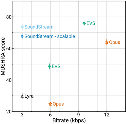More recently, Fig. 1: SoundStream @ 3 kbps vs. state-of-the-art codecs. <details> <summary>Image 1 Details</summary>  ### Visual Description ## Scatter Plot: MUSHRA Score vs. Bitrate (kbps) ### Overview The image is a scatter plot comparing audio codec performance using MUSHRA scores (y-axis) against bitrate (x-axis). Five data points represent different audio systems: SoundStream, SoundStream - scalable, EVS, Opus, and Lyra. The plot highlights trade-offs between compression efficiency (bitrate) and perceived quality (MUSHRA score). ### Components/Axes - **X-axis (Bitrate)**: Labeled "Bitrate (kbps)" with values from 3 to 12 kbps. - **Y-axis (MUSHRA Score)**: Labeled "MUSHRA score" with values from 20 to 80. - **Legend**: Located in the top-left corner, mapping symbols to systems: - Blue square: SoundStream - Blue circle: SoundStream - scalable - Green diamond: EVS - Orange star: Opus - Black triangle: Lyra ### Detailed Analysis - **SoundStream**: - Blue square at (3 kbps, 70 MUSHRA). - Blue circle (scalable version) at (3 kbps, 65 MUSHRA). - **EVS**: - Green diamond at (6 kbps, 50 MUSHRA). - Green diamond at (9 kbps, 75 MUSHRA). - **Opus**: - Orange star at (12 kbps, 65 MUSHRA). - Orange star at (12 kbps, 25 MUSHRA). - **Lyra**: - Black triangle at (3 kbps, 30 MUSHRA). ### Key Observations 1. **Bitrate-Quality Trade-off**: Higher bitrates generally correlate with higher MUSHRA scores (e.g., EVS at 9 kbps scores 75 vs. 50 at 6 kbps). 2. **Outliers**: - Opus at 12 kbps has two divergent scores (65 and 25), suggesting variability in performance under specific conditions. - Lyra consistently underperforms, with the lowest score (30) at the lowest bitrate (3 kbps). 3. **Scalability Impact**: SoundStream - scalable (blue circle) scores 5 MUSHRA points lower than the non-scalable version at the same bitrate. ### Interpretation The plot demonstrates that codec efficiency and quality vary significantly. Efficient codecs like Opus and EVS achieve competitive scores at lower bitrates, but Opus shows inconsistency at 12 kbps. Lyra’s low scores indicate inferior quality or higher compression artifacts. The scalable version of SoundStream sacrifices some quality for adaptability, while EVS maintains higher scores at mid-to-high bitrates. The data underscores the importance of balancing bitrate constraints with perceptual quality in audio encoding. </details> machine learning models have been successfully applied in the field of audio compression, demonstrating the additional value brought by data-driven solutions. For example, it is possible to apply them as a post-processing step to improve the quality of existing codecs. This can be accomplished either via audio superresolution, i.e., extending the frequency bandwidth [1], via audio denoising, i.e., removing lossy coding artifacts [2], or via packet loss concealment [3]. Other solutions adopt ML-based models as an integral part of the audio codec architecture. In these areas, recent advances in text-to-speech (TTS) technology proved to be a key ingredient. For example, WaveNet [4], a strong generative model originally applied to generate speech from text, was adopted as a decoder in a neural codec [5], [6]. Other neural audio codecs adopt different model architectures, e.g., WaveRNN in LPCNet [7] and WaveGRU in Lyra [8], all targeting speech at low bitrates. 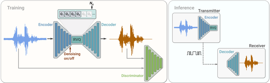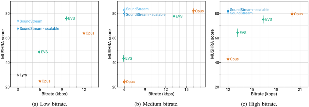In this paper we propose SoundStream , a novel audio codec that can compress speech, music and general audio more efficiently than previous codecs, as illustrated in Figure 1. SoundStream leverages state-of-the-art solutions in the field of neural audio synthesis, and introduces a new learnable quantization module, to deliver audio at high perceptual quality, while operating at low-to-medium bitrates. Figure 2 illustrates the high level model architecture of the codec. A fully convolutional encoder receives as input a time-domain waveform and produces a sequence of embeddings at a lower sampling rate, which are quantized by a residual vector quantizer. A fully convolutional decoder receives the quantized embeddings and reconstructs an approximation of the original waveform. The model is trained end-to-end using both reconstruction and Fig. 2: SoundStream model architecture. A convolutional encoder produces a latent representation of the input audio samples, which is quantized using a variable number n q of residual vector quantizers (RVQ). During training, the model parameters are optimized using a combination of reconstruction and adversarial losses. An optional conditioning input can be used to indicate whether background noise has to be removed from the audio. When deploying the model, the encoder and quantizer on a transmitter client send the compressed bitstream to a receiver client that can then decode the audio signal. <details> <summary>Image 2 Details</summary>  ### Visual Description ## Diagram: Audio Signal Processing System Architecture ### Overview The image depicts a dual-phase system architecture for audio signal processing, divided into **Training** and **Inference** workflows. The system employs an encoder-decoder framework with residual vector quantization (RVQ) and adversarial training components. ### Components/Axes #### Training Workflow 1. **Encoder**: - Input: Blue waveform labeled "Encoder" - Output: Quantized residual vectors (Q₁ to Qₙ) - Position: Left side, connected to RVQ block 2. **RVQ (Residual Vector Quantization)**: - Central block with denoising toggle (on/off) - Processes quantized residuals 3. **Decoder**: - Input: Processed residuals from RVQ - Output: Reconstructed waveform (orange) - Position: Right side of RVQ 4. **Discriminator**: - Green pyramid-shaped component - Receives output from Decoder - Position: Bottom-right of Training section #### Inference Workflow 1. **Transmitter**: - Encoder with RVQ (blue waveform input) - Output: Quantized signal - Position: Top-left of Inference section 2. **Channel**: - Dotted line with noise pattern (squiggle) - Connects Transmitter to Receiver 3. **Receiver**: - Decoder (orange waveform output) - Position: Bottom-right of Inference section ### Detailed Analysis - **Training Flow**: - Original audio (blue) → Encoder → RVQ (quantization with denoising control) → Decoder → Reconstructed audio (orange) - Discriminator evaluates reconstruction quality, suggesting GAN-like adversarial training - **Inference Flow**: - Audio encoded via Transmitter (Encoder + RVQ) → Noisy transmission → Decoder in Receiver reconstructs signal - **Color Coding**: - Blue: Original/transmitted waveforms - Orange: Reconstructed/received waveforms - Green: Discriminator component ### Key Observations 1. **Denoising Toggle**: RVQ block includes explicit denoising control, indicating adaptive processing. 2. **Adversarial Training**: Discriminator's presence implies quality assessment during training. 3. **Channel Noise**: Dotted line in Inference represents real-world transmission imperfections. 4. **Component Reuse**: Encoder/Decoder architecture is shared between Training and Inference phases. ### Interpretation This architecture demonstrates a hybrid approach combining: 1. **Compression**: Through RVQ for efficient residual representation 2. **Quality Control**: Via discriminator for perceptual fidelity 3. **Robustness**: By simulating channel noise in inference 4. **Adaptability**: Denoising toggle suggests context-aware processing The system appears designed for applications requiring high-fidelity audio reconstruction under bandwidth constraints, with training focused on both compression efficiency and perceptual quality. The discriminator's role suggests potential use in scenarios where subjective audio quality is critical, such as voice assistants or music streaming. </details> adversarial losses. To this end, one (or more) discriminators are trained jointly, with the goal of distinguishing the decoded audio from the original audio and, as a by-product, provide a space where a feature-based reconstruction loss can be computed. Both the encoder and the decoder only use causal convolutions, so the overall architectural latency of the model is determined solely by the temporal resampling ratio between the original time-domain waveform and the embeddings. In summary, this paper makes the following key contributions: - We propose SoundStream , a neural audio codec in which all the constituent components (encoder, decoder and quantizer) are trained end-to-end with a mix of reconstruction and adversarial losses to achieve superior audio quality. - We introduce a new residual vector quantizer, and investigate the rate-distortion-complexity trade-offs implied by its design. In addition, we propose a novel 'quantizer dropout' technique for training the residual vector quantizer, which enables a single model to handle different bitrates. - We demonstrate that learning the encoder brings a very significant coding efficiency improvement, with respect to a solution that adopts mel-spectrogram features. - We demonstrate by means of subjective quality metrics that SoundStream outperforms both Opus and EVS over a wide range of bitrates. - We design our model to support streamable inference, which can operate at low-latency. When deployed on a smartphone, it runs in real-time on a single CPU thread. - We propose a variant of the SoundStream codec that performs jointly audio compression and enhancement, without introducing additional latency. ## II. RELATED WORK Traditional audio codecs - Opus [9] and EVS [10] are state-of-the-art audio codecs, which combine traditional coding tools, such as LPC, CELP and MDCT, to deliver high coding efficiency over different content types, bitrates and sampling rates, while ensuring low-latency for real-time audio communications. We compare SoundStream with both Opus and EVS in our subjective evaluation. Audio generative models -Several generative models have been developed for converting text or coded features into audio waveforms. WaveNet [4] allows for global and local signal conditioning to synthesize both speech and music. SampleRNN [11] uses recurrent networks in a similar fashion, but it relies on previous samples at different scales. These auto-regressive models deliver very high-quality audio, at the cost of increased computational complexity, since samples are generated one by one. To overcome this issue, Parallel WaveNet [12] allows for parallel computation, yielding considerable speedup during inference. Other approaches involve lightweight and sparse models [13] and networks mimicking the fast Fourier transform as part of the model [7], [14]. More recently, generative adversarial models have emerged as a solution able to deliver high-quality audio with a lower computational complexity. MelGAN [15] is trained to produce audio waveforms when conditioned on mel-spectrograms, training a multi-scale waveform discriminator together with the generator. HiFiGAN [16] takes a similar approach but it applies discriminators to both multiple scales and multiple periods of the audio samples. The design of the decoder and the losses in SoundStream is based on this class of audio generative models. Audio enhancement - Deep neural networks have been applied to different audio enhancement tasks, ranging from denoising [17]-[21] to dereverberation [22], [23], lossy coding denoising [2] and frequency bandwidth extension [1], [24]. In this paper we show that it is possible to jointly perform audio enhancement and compression with a single model, without introducing additional latency. Vector quantization - Learning the optimal quantizer is a key element to achieve high coding efficiency. Optimal scalar quantization based on Lloyd's algorithm [25] can be extended to a high-dimensional space via the generalized Lloyd algorithm (GLA) [26], which is very similar to k-means clustering [27]. In vector quantization [28], a point in a high-dimensional space is mapped onto a discrete set of code vectors. Vector quantization has been commonly used as a building block of traditional audio codecs [29]. For example, CELP [30] adopts an excitation signal encoded via a vector quantizer codebook. More recently, vector quantization has been applied in the context of neural network models to compress the latent representation of input features. For example, in variational autoencoders, vector quantization has been used to generate images [31], [32] and music [33], [34]. Vector quantization can become prohibitively expensive, as the size of the codebook grows exponentially when rate is increased. For this reason, structured vector quantizers [35], [36] (e.g., residual, product, lattice vector quantizers, etc.) have been proposed to obtain a trade-off between computational complexity and coding efficiency in traditional codecs. In SoundStream , we extend the learnable vector quantizer of VQ-VAE [31] and introduce a residual (a.k.a. multi-stage) vector quantizer, which is learned end-to-end with the rest of the model. To the best of the authors knowledge, this is the first time that this form of vector quantization is used in the context of neural networks and trained end-to-end with the rest of the model. Neural audio codecs - End-to-end neural audio codecs rely on data-driven methods to learn efficient audio representations, instead of relying on handcrafted signal processing components. Autoencoder networks with quantization of hidden features were applied to speech coding early on [37]. More recently, a more sophisticated deep convolutional network for speech compression was described in [38]. Efficient compression of audio using neural networks has been demonstrated in several works, mostly targeting speech coding at low bitrates. A VQVAE speech codec was proposed in [6], operating at 1 . 6 kbps. Lyra [8] is a generative model that encodes quantized melspectrogram features of speech, which are decoded with an auto-regressive WaveGRU model to achieve state-of-the-art results at 3 kbps. A very low-bitrate codec was proposed in [39] by decoding speech representations obtained via self-supervised learning. An end-to-end audio codec targeting general audio at high bitrates (i.e., above 64 kbps) was proposed in [40]. The model architecture adopts a residual coding pipeline, which consists of multiple autoencoding modules and a psychoacoustic model is used to drive the loss function during training. Unlike [39] which specifically targets speech by combining speaker, phonetic and pitch embeddings, SoundStream does not make assumptions on the nature of the signal it encodes, and thus works for diverse audio content types. While [8] learns a decoder on fixed features, SoundStream is trained in an end-to-end fashion. Our experiments (see Section IV) show that learning the encoder increases the audio quality substantially. SoundStream achieves bitrate scalability, i.e., the ability of a single model to operate at different bitrates at no additional cost, thanks to its residual vector quantizer and to our original quantizer dropout training scheme (see Section III-C). This is unlike [38] and [40] which enforce a specific bitrate during training and require training a different model for each target bitrate. A single SoundStream model is able to compress speech, music and general audio, while operating at a 24 kHz sampling rate and low-to-medium bitrates ( 3 kbps to 18 kbps in our experiments), in real time on a smartphone CPU. This is the first time that a neural audio codec is shown to outperform state-of-the-art codecs like Opus and EVS over this broad range of bitrates. Joint compression and enhancement - Recent work has explored joint compression and enhancement. The work in [41] trains a speech enhancement system with a quantized bottleneck. Instead, SoundStream integrates a time-dependent conditioning layer, which allows for real-time controllable denoising. As we design SoundStream as a general-purpose audio codec, controlling when to denoise allows for encoding acoustic scenes and natural sounds that would be otherwise removed. ## III. MODEL We consider a single channel recording x ∈ R T , sampled at f s . The SoundStream model consists of a sequence of three building blocks, as illustrated in Figure 2: - an encoder, which maps x to a sequence of embeddings (see Section III-A), - a residual vector quantizer, which replaces each embedding by the sum of vectors from a set of finite codebooks, thus compressing the representation with a target number of bits (see Section III-C), - a decoder, which produces a lossy reconstruction ˆ x ∈ R T from quantized embeddings (see Section III-B). The model is trained end-to-end together with a discriminator (see Section III-D), using the mix of adversarial and reconstruction losses described in Section III-E. Optionally, a conditioning signal can be added, which determines whether denoising is applied at the encoder or decoder side, as detailed in Section III-F. ## A. 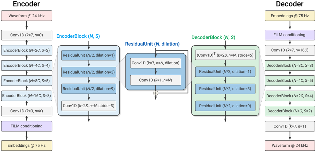Encoder architecture The encoder architecture is illustrated in Figure 3 and follows the same structure as the streaming SEANet encoder described in [1], but without skip connections. It consists of a 1D convolution layer (with C enc channels), followed by B enc convolution blocks. Each of the blocks consists of three residual units, containing dilated convolutions with dilation rates of 1, 3, and 9, respectively, followed by a down-sampling layer in the form of a strided convolution. The number of channels is doubled whenever down-sampling, starting from C enc. A final 1D convolution layer with a kernel of length 3 and a stride of 1 is used to set the dimensionality of the embeddings to D . To guarantee real-time inference, all convolutions are causal . This means that padding is only applied to the past but not the future in both training and offline inference, whereas no padding is used in streaming inference. We use the ELU activation [42] and we do not apply any normalization. The number B enc of convolution blocks and the corresponding striding sequence determines the temporal resampling ratio between the input waveform and the embeddings. For example, when B enc = 4 and using (2 , 4 , 5 , 8) as strides, one embedding is computed every M = 2 · 4 · 5 · 8 = 320 input samples. Thus, the encoder outputs enc ( x ) ∈ R S × D , with S = T/M . <details> <summary>Image 3 Details</summary>  ### Visual Description ## Block Diagram: Audio Processing Neural Network Architecture ### Overview The diagram illustrates a neural network architecture for audio processing, featuring an encoder-decoder structure with residual units and film conditioning. The system processes audio waveforms at 24 kHz, with embeddings at 75 Hz, and includes multiple convolutional and residual blocks with specific dilation patterns. ### Components/Axes **Key Components:** 1. **Encoder Section (Left Side)** - Input: Waveform @ 24 kHz - Initial Layer: Conv1D (k=7, n=C) - EncoderBlocks: - EncoderBlock (N=2C, S=2) - EncoderBlock (N=4C, S=4) - EncoderBlock (N=8C, S=5) - EncoderBlock (N=16C, S=8) - Final Encoder Layer: Conv1D (k=3, n=K) - Film Conditioning: Embeddings @ 75 Hz 2. **Residual Unit (Center)** - Structure: - ResidualUnit (N/2, dilation=1) - ResidualUnit (N/2, dilation=3) - ResidualUnit (N/2, dilation=9) - Core Operations: - Conv1D (k=7, n=K) - Conv1D (k=3, n=N) 3. **Decoder Section (Right Side)** - Input: Embeddings @ 75 Hz - Film Conditioning - DecoderBlocks (reverse order of encoder): - DecoderBlock (N=16C, S=8) - DecoderBlock (N=8C, S=5) - DecoderBlock (N=4C, S=4) - DecoderBlock (N=2C, S=2) - Final Output: Waveform @ 24 kHz **Parameter Notation:** - `k`: Kernel size - `n`: Number of channels - `C`: Channel multiplier - `S`: Stride - `K`: Final channel count - `N`: Base channel count ### Detailed Analysis **Encoder Flow:** 1. Starts with 24 kHz waveform input 2. Initial Conv1D (k=7, n=C) reduces temporal resolution 3. Four EncoderBlocks progressively increase channel count (2C→4C→8C→16C) while reducing temporal resolution via stride (S=2→4→5→8) 4. Final Conv1D (k=3, n=K) prepares for residual unit input **Residual Unit:** - Implements dilated convolutions with increasing dilation factors (1→3→9) - Core operations: - 7x7 Conv1D (k=7, n=K) with dilation=1 - 3x3 Conv1D (k=3, n=N) with dilation=3 - 1x1 Conv1D (k=1, n=N) with dilation=9 - Output combines all residual paths **Decoder Flow:** 1. Starts with 75 Hz embeddings 2. Film conditioning adapts normalization parameters 3. Four DecoderBlocks reverse the encoder process: - Channel reduction (16C→8C→4C→2C) - Temporal upsampling via stride (S=8→5→4→2) 4. Final Conv1D (k=7, n=1) produces 24 kHz output waveform ### Key Observations 1. **Symmetric Architecture**: Encoder/Decoder mirror each other with reversed channel counts and strides 2. **Dilation Pattern**: Residual unit uses 1→3→9 dilation for multi-scale feature capture 3. **Channel Progression**: - Encoder: C→2C→4C→8C→16C - Decoder: 16C→8C→4C→2C 4. **Temporal Resolution**: - Encoder: 24 kHz → 12 kHz → 6 kHz → 3 kHz → 1.5 kHz - Decoder: 1.5 kHz → 3 kHz → 6 kHz → 12 kHz → 24 kHz 5. **Film Conditioning**: 75 Hz embeddings modulate network behavior throughout ### Interpretation This architecture appears to be a modified U-Net for audio processing, combining: - **Residual Learning**: Through skip connections in encoder/decoder - **Dilated Convolutions**: For capturing long-range dependencies - **Multi-scale Processing**: Via progressive channel expansion/contraction - **Conditioning Mechanism**: 75 Hz embeddings likely provide content-specific guidance The use of 7x7 and 3x3 kernels suggests a focus on capturing both local and global audio features. The 24 kHz input/output indicates standard telephone-quality audio processing, while 75 Hz embeddings might represent prosodic or spectral features for conditioning. </details> Fig. 3: Encoder and decoder model architecture. <details> <summary>Image 4 Details</summary>  ### Visual Description ## Pseudocode: Residual Vector Quantization Algorithm ### Overview This pseudocode describes a quantization algorithm that iteratively applies a series of quantizers to an input vector `y` (output of an encoder) to produce a quantized output `ŷ`. The process involves updating a residual vector at each step to refine the quantization. ### Components/Axes - **Input**: - `y = enc(x)`: Output of an encoder function `enc` applied to input `x`. - `Q_i` for `i = 1..N_q`: A vector of `N_q` quantizers, where each quantizer `Q_i` operates on the residual vector. - **Output**: - `ŷ`: The final quantized vector. ### Detailed Analysis 1. **Initialization**: - `ŷ ← 0.0`: Initialize the quantized output to zero. - `residual ← y`: Set the initial residual to the encoder output `y`. 2. **Iterative Quantization**: For each quantizer `Q_i` (from `i = 1` to `N_q`): - Update `ŷ` by adding the result of applying `Q_i` to the current residual: `ŷ += Q_i(residual)`. - Update the residual by subtracting the quantized value from the current residual: `residual -= Q_i(residual)`. 3. **Termination**: Return the final quantized vector `ŷ`. ### Key Observations - The algorithm processes the input vector `y` sequentially through `N_q` quantizers, refining the quantization at each step. - The residual vector is progressively reduced, ensuring that each quantizer operates on the remaining unquantized portion of `y`. - The final output `ŷ` is a cumulative sum of quantized residuals from all `Q_i`. ### Interpretation This algorithm is likely used in scenarios requiring efficient quantization of high-dimensional data (e.g., in neural network compression or signal processing). By iteratively applying quantizers to the residual, it balances quantization error across multiple stages, potentially improving the quality of the quantized representation compared to a single-stage quantization. The use of a residual ensures that earlier quantization steps do not dominate the final result, allowing finer adjustments in later stages. No numerical values or trends are present in the image, as it describes an algorithm rather than data. </details> | Algorithm 1: Residual Vector Quantization | |---------------------------------------------------------------------------------------| | Input: y = enc ( x ) the output of the encoder, vector quantizers Q i for i = 1 ..N q | | Output: the quantized ˆ y ˆ y ← 0 . 0 residual ← y for i = 1 to N q do | ## B. Decoder architecture The decoder architecture follows a similar design, as illustrated in Figure 3. A 1D convolution layer is followed by a sequence of B dec convolution blocks. The decoder block mirrors the encoder block, and consists of a transposed convolution for up-sampling followed by the same three residual units. We use the same strides as the encoder, but in reverse order, to reconstruct a waveform with the same resolution as the input waveform. The number of channels is halved whenever upsampling, so that the last decoder block outputs C dec channels. A final 1D convolution layer with one filter, a kernel of size 7 and stride 1 projects the embeddings back to the waveform domain to produce ˆ x . In Figure 3, the same number of channels in both the encoder and the decoder is controlled by the same parameter, i.e., C enc = C dec = C . We also investigate cases in which C enc = C dec, which results in a computationally lighter encoder and a heavier decoder, or vice-versa (see Section V-D). ## C. Residual Vector Quantizer: The goal of the quantizer is to compress the output of the encoder enc ( x ) to a target bitrate R , expressed in bits/second (bps). In order to train SoundStream in an endto-end fashion, the quantizer needs to be jointly trained with the encoder and the decoder by backpropagation. The vector quantizer (VQ) proposed in [31], [32] in the context of VQVAEs meets this requirement. This vector quantizer learns a codebook of N vectors to encode each D -dimensional frame of enc ( x ) . The encoded audio enc ( x ) ∈ R S × D is then mapped to a sequence of one-hot vectors of shape S × N , which can be represented using S log 2 N bits. Limitations of Vector Quantization - As a concrete example, let us consider a codec targeting a bitrate R = 6000 bps. When using a striding factor M = 320 , each second of audio at sampling rate f s = 24000 Hz is represented by S = 75 frames at the output of the encoder. This corresponds to r = 6000 / 75 = 80 bits allocated to each frame. Using a plain vector quantizer, this requires storing a codebook with N = 2 80 vectors, which is obviously unfeasible. 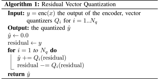Residual Vector Quantizer -To address this issue we adopt a Residual Vector Quantizer (a.k.a. multi-stage vector quantizer [36]), which cascades N q layers of VQ as follows. The unquantized input vector is passed through a first VQ and quantization residuals are computed. The residuals are then iteratively quantized by a sequence of additional N q -1 vector quantizers, as described in Algorithm 1. The total rate budget is uniformly allocated to each VQ, i.e., r i = r/N q = log 2 N . For example, when using N q = 8 , each quantizer uses a codebook of size N = 2 r/N q = 2 80 / 8 = 1024 . For a target rate budget r , the parameter N q controls the tradeoff between computational complexity and coding efficiency, which we investigate in Section V-D. The codebook of each quantizer is trained with exponential moving average updates, following the method proposed in VQ-VAE-2 [32]. To improve the usage of the codebooks we use two additional methods. First, instead of using a random initialization for the codebook vectors, we run the k-means algorithm on the first training batch and use the learned centroids as initialization. This allows the codebook to be close to the distribution of its inputs and improves its usage. Second, as proposed in [34], when a codebook vector has not been assigned any input frame for several batches, we replace it with an input frame randomly sampled within the current batch. More precisely, we track the exponential moving average of the assignments to each vector (with a decay factor of 0 . 99 ) and replace the vectors of which this statistic falls below 2 . Enabling bitrate scalability with quantizer dropout - Residual vector quantization provides a convenient framework for controlling the bitrate. For a fixed size N of each codebook, the number of VQ layers N q determines the bitrate. Since the vector quantizers are trained jointly with the encoder/decoder, in principle a different SoundStream model should be trained for each target bitrate. Instead, having a single bitrate scalable model that can operate at several target bitrates is much more practical, since this reduces the memory footprint needed to store model parameters both at the encoder and decoder side. To train such a model, we modify Algorithm 1 in the following way: for each input example, we sample n q uniformly at random in [1; N q ] and only use quantizers Q i for i = 1 . . . n q . This can be seen as a form of structured dropout [43] applied to quantization layers. Consequently, the model is trained to encode and decode audio for all target bitrates corresponding to the range n q = 1 . . . N q . During inference, the value of n q is selected based on the desired bitrate. Previous models for neural compression have relied on product quantization (wav2vec 2.0 [44]), or on concatenating the output of several VQ layers [5], [6]. With such approaches, changing the bitrate requires either changing the architecture of the encoder and/or the decoder, as the dimensionality changes, or retraining an appropriate codebook. A key advantage of our residual vector quantizer is that the dimensionality of the embeddings does not change with the bitrate. Indeed, the additive composition of the outputs of each VQ layer progressively refines the quantized embeddings, while keeping the same shape. Hence, no architectural changes are needed in neither the encoder nor the decoder to accommodate different bitrates. In Section V-C, we show that this method allows one to train a single SoundStream model, which matches the performance of models trained specifically for a given bitrate. ## D. 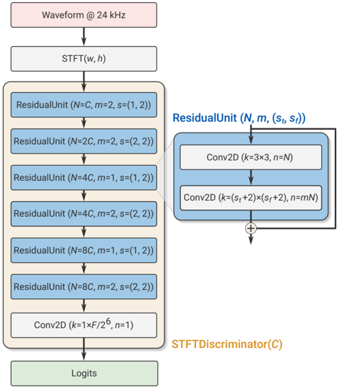Discriminator architecture To compute the adversarial losses described in Section III-E, we define two different discriminators: i) a wave-based discriminator, which receives as input a single waveform; ii) an STFT-based discriminator, which receives as input the complexvalued STFT of the input waveform, expressed in terms of real and imaginary parts. Since both discriminators are fully convolutional, the number of logits in the output is proportional to the length of the input audio. For the wave-based discriminator, we use the same multiresolution convolutional discriminator proposed in [15] and adopted in [45]. Three structurally identical models are applied to the input audio at different resolutions: original, 2-times Fig. 4: STFT-based discriminator architecture. <details> <summary>Image 5 Details</summary>  ### Visual Description ## Diagram: Audio Signal Processing Pipeline with Neural Network Architecture ### Overview The diagram illustrates a neural network architecture for audio signal processing, starting with a 24 kHz waveform input. It includes a Short-Time Fourier Transform (STFT) for time-frequency representation, followed by a series of residual units and convolutional layers, culminating in logits for classification or regression. The architecture incorporates residual connections and a discriminator component, suggesting potential use in generative or discriminative tasks. ### Components/Axes 1. **Input**: Waveform @ 24 kHz (time-domain audio signal). 2. **STFT (w, h)**: Converts the waveform into a time-frequency representation (spectrogram). 3. **Residual Units**: Stacked layers with parameters: - `N`: Number of channels/filters (e.g., 2, 4, 8, 16). - `C`: Input channels (e.g., 2, 2, 2, 2). - `m`: Scale factor (e.g., 1, 2). - `s`: Stride (e.g., 1, 2). - `t`: Kernel size (e.g., 2, 2). 4. **Conv2D Layers**: - `k=3×3`, `n=N`: Standard convolution with kernel size 3×3. - `k=(s_i+2)×(s_f+2)`, `n=mN`: Adaptive kernel size based on stride and scale. 5. **STFT Discriminator (C)**: Likely a discriminator network for evaluating audio quality (e.g., in a GAN). 6. **Logits**: Final output layer for classification/regression. ### Detailed Analysis - **Residual Units**: - The first unit (`N=2, C=2, s=1, t=2`) processes the STFT output with minimal downsampling. - Subsequent units increase `N` (e.g., 4, 8, 16) and adjust `s`/`t` to control feature extraction granularity. - Parameters like `m=1` (no scaling) and `m=2` (doubling channels) suggest dynamic channel adjustment. - **Conv2D Layers**: - Early layers use fixed `k=3×3` for local feature extraction. - Later layers adapt kernel sizes (`k=(s_i+2)×(s_f+2)`) to match stride and scale, enabling hierarchical feature learning. - **STFT Discriminator (C)**: Positioned after the residual units, it likely evaluates the processed audio's fidelity or authenticity. - **Logits**: Output layer with no activation function, indicating raw scores for downstream tasks (e.g., softmax for classification). ### Key Observations - **Hierarchical Feature Learning**: Residual units and adaptive Conv2D layers enable multi-scale feature extraction. - **Residual Connections**: Facilitate gradient flow, critical for training deep networks. - **STFT Integration**: Time-frequency domain processing is central to audio tasks. - **Discriminator Role**: Suggests a generative component (e.g., GAN) for audio synthesis or enhancement. ### Interpretation This architecture is designed for audio processing tasks such as classification, denoising, or generation. The STFT converts raw audio into a spectrogram, which is then processed through residual blocks to capture temporal and spectral features. The increasing `N` values in residual units indicate progressive feature complexity, while the discriminator implies a focus on audio quality or authenticity. The logits output suggests the model is tailored for supervised learning, though the absence of an activation function leaves the final task ambiguous (e.g., regression vs. classification). The use of adaptive kernel sizes in Conv2D layers highlights flexibility in handling varying input resolutions. </details> down-sampled, and 4-times down-sampled. Each single-scale discriminator consists of an initial plain convolution followed by four grouped convolutions, each of which has a group size of 4, a down-sampling factor of 4, and a channel multiplier of 4 up to a maximum of 1024 output channels. They are followed by two more plain convolution layers to produce the final output, i.e., the logits. The STFT-based discriminator is illustrated in Figure 4 and operates on a single scale, computing the STFT with a window length of W = 1024 samples and a hop length of H = 256 samples. A 2D-convolution (with kernel size 7 × 7 and 32 channels) is followed by a sequence of residual blocks. Each block starts with a 3 × 3 convolution, followed by a 3 × 4 or a 4 × 4 convolution, with strides equal to (1 , 2) or (2 , 2) , where ( s t , s f ) indicates the down-sampling factor along the time axis and the frequency axis. We alternate between (1 , 2) and (2 , 2) strides, for a total of 6 residual blocks. The number of channels is progressively increased with the depth of the network. At the output of the last residual block, the activations have shape T/ ( H · 2 3 ) × F/ 2 6 , where T is the number of samples in the time domain and F = W/ 2 is the number of frequency bins. The last layer aggregates the logits across the (down-sampled) frequency bins with a fully connected layer (implemented as a 1 × F/ 2 6 convolution), to obtain a 1-dimensional signal in the (down-sampled) time domain. ## E. Training objective Let G ( x ) = dec ( Q ( enc ( x )) denote the SoundStream generator, which processes the input waveform x through the encoder, the quantizer and the decoder, and ˆ x = G ( x ) be the decoded waveform. We train SoundStream with a mix of losses to achieve both signal reconstruction fidelity and perceptual quality, following the principles of the perception-distortion trade-off discussed in [46]. The adversarial loss is used to promote perceptual quality and it is defined as a hinge loss over the logits of the discriminator, averaged over multiple discriminators and over time. More formally, let k ∈ { 0 , . . . , K } index over the individual discriminators, where k = 0 denotes the STFT-based discriminator and k ∈ { 1 , . . . , K } the different resolutions of the waveform-based discriminator ( K = 3 in our case). Let T k denote the number of logits at the output of the k -th discriminator along the time dimension. The discriminator is trained to classify original vs. decoded audio, by minimizing $$L _ { D } = E _ { x } \left[ \frac { 1 } { K } \sum _ { k = 1 } ^ { K } \frac { 1 } { T _ { k } } \sum _ { t } ^ { m } max ( 0 , 1 - D _ { k , t } ( x ) ) \right] + E _ { x } \left[ \frac { 1 } { K } \sum _ { k = 1 } ^ { K } \frac { 1 } { T _ { k } } \sum _ { t } ^ { m } max ( 0 , 1 + D _ { k , t } ( G ( x ) ) \right] . (1)$$ while the adversarial loss for the generator is $$\begin{aligned} L _ { G } = E _ { x } \left[ \frac { 1 } { K } \sum _ { k , t } ^ { 1 } 1 _ { T _ { k } } max ( 0 , 1 - D _ { k , t } ( G ( x ) ) \right] \cdot ( 2 ) & \text{consist} \\ & \text{When } \left( 0 , 1 - D _ { k , t } ( G ( x ) ) \right) \text{ denotes } \\ & \text{compo} \end{aligned}$$ To promote fidelity of the decoded signal ˆ x with respect to the original x we adopt two additional losses: i) a 'feature' loss L feat G , computed in the feature space defined by the discriminator(s) [15]; ii) a multi-scale spectral reconstruction loss L rec G [47]. More specifically, the feature loss is computed by taking the average absolute difference between the discriminator's internal layer outputs for the generated audio and those for the corresponding target audio. $$\begin{array}{ll} L_{G}^{feat} = E_{x} \left[ \frac{1}{\sum _{k,l} T_{kl}} \sum _{i=1}^K D^{k,t}( x ) - D^{k,t}( G( x )) \right] , & \text{where } I \text{ is the number of internal layers } D^{(0)}( f ) \text{ takes a } (3) \text{ coefficient }$$ where L is the number of internal layers, D ( l ) k,t ( l ∈ { 1 , . . . , L } ) is the t -th output of layer l of discriminator k , and T k,l denotes the length of the layer in the time dimension. The multi-scale spectral reconstruction loss follows the specifications described in [48]: where S s t ( x ) denotes the t -th frame of a 64-bin melspectrogram computed with window length equal to s and hop length equal to s/ 4 . We set α s = √ s/ 2 as in [48]. The overall generator loss is a weighted sum of the different loss components: $$\begin{aligned} & L G = \lambda _ { adv } L G + \lambda _ { feat } \cdot L \\ & ( 6 ) W e G ^ { \prime } + \lambda _ { rec } \cdot L G \cdot ( 6 ) W e G ^ { \prime } \end{aligned}$$ In all our experiments we set λ adv = 1 , λ feat = 100 and λ rec = 1 . ## F. Joint compression and enhancement In traditional audio processing pipelines, compression and enhancement are typically performed by different modules. For example, it is possible to apply an audio enhancement algorithm at the transmitter side, before audio is compressed, or at the receiver side, after audio is decoded. In this setup, each processing step contributes to the end-to-end latency, e.g., due to buffering the input audio to the expected frame length determined by the specific algorithm adopted. Conversely, we design SoundStream in such a way that compression and enhancement can be carried out jointly by the same model, without increasing the overall latency. The nature of the enhancement can be determined by the choice of the training data. As a concrete example, in this paper we show that it is possible to combine compression with background noise suppression. More specifically, we train a model in such a way that one can flexibly enable or disable denoising at inference time, by feeding a conditioning signal that represents the two modes (denoising enabled or disabled). To this end, we prepare the training data to consist of tuples of the form: ( inputs , targets , denoise ) . When denoise = false , targets = inputs ; when denoise = true , targets contain the clean speech component of the corresponding inputs . Hence, the network is trained to reconstruct noisy speech if the conditioning signal is disabled, and to produce a clean version of the noisy input if it is enabled. Note that when inputs consist of clean audio (speech or music), targets = inputs and denoise can be either true or false . This is done to prevent SoundStream from adversely affecting clean audio when denoising is enabled. To process the conditioning signal, we use Feature-wise Linear Modulation (FiLM) layers [49] in between residual units, which take network features as inputs and transform them as $$\overrightarrow { a _ { n } , c } = \gamma _ { n } \overrightarrow { a _ { n } , c } + \beta _ { n }$$ where a n,c is the n th activation in the c th channel. The coefficients γ n,c and β n,c are computed by a linear layer that takes as input a (potentially time-varying) two-dimensional one-hot encoding that determines the denoising mode. This allows one to adjust the level of denoising over time. In principle, FiLM layers can be used anywhere throughout the encoder and decoder architecture. However, in our preliminary experiments, we found that applying conditioning at the bottleneck either at the encoder or at the decoder side (as illustrated in Figure 3) was effective and no further improvements were observed by applying FiLM layers at different depths. In Section V-E, we quantify the impact of enabling denoising at either the encoder or decoder side both in terms of audio quality and bitrate. ## IV. EVALUATION SETUP ## A. Datasets We train SoundStream on three types of audio content: clean speech, noisy speech and music, all at 24 kHz sampling rate. For clean speech, we use the LibriTTS dataset [50]. For noisy speech, we synthesize samples by mixing speech from LibriTTS with noise from Freesound [51]. We apply peak normalization to randomly selected crops of 3 seconds and adjust the mixing gain of the noise component sampling uniformly in the interval [ -30 dB , 0 dB ] . For music, we use the MagnaTagATune dataset [52]. We evaluate our models on disjoint test splits of the datasets above. In addition, we collected a real-world dataset, which contains both near-field and far-field (reverberant) speech, with background noise in some of the examples. Unless stated otherwise, objective and subjective metrics are computed on a set of 200 audio clips 2-4 seconds long, with 50 samples from each of the four datasets listed above (i.e., clean speech, noisy speech, music, noisy/reverberant speech). ## B. Evaluation metrics To evaluate SoundStream , we perform subjective evaluations by human raters. We have chosen a crowd-sourced methodology inspired by MUSHRA [53], with a hidden reference but no lowpass-filtered anchor. Each of the 200 samples of the evaluation dataset, which include clean, noisy and reverberant speech, as well as music, was rated 20 times. The raters were required to be native English speakers and be using headphones. Additionally, to avoid noisy data, a post-screening was put in place to exclude ratings by listeners who rated the reference below 90 more than 20% of the time or rated non-reference samples above 90 more than 50% of the time. For development and hyperparameter selection, we rely on computational, objective metrics. Numerous metrics have been developed in the past for assessing the perceived similarity between a reference and a processed audio signal. The ITU-T standards PESQ [54] and its replacement POLQA [55] are commonly used metrics. However, both are inconvenient to use owing to licensing restrictions. We choose the freely available and recently open-sourced ViSQOL [56], [57] metric, which has previously shown comparable performance to POLQA. In early experiments, we found this metric to be strongly correlated with subjective evaluations. We thus use it for model selection and ablation studies. ## C. Baselines Opus [9] is a versatile speech and audio codec supporting signal bandwidths from 4 kHz to 24 kHz and bitrates from 6 kbps to 510 kbps. Since its standardization by the IETF in 2012 it has been widely deployed for speech communication over the internet. As the audio codec in applications such as Zoom and applications based on WebRTC [58], [59], such as Microsoft Teams and Google Meet, Opus has hundreds of millions of daily users. Opus is also one of the main audio codecs used in YouTube for streaming. Enhanced Voice Services (EVS) [10] is the latest codec standardized by the 3GPP and was primarily designed for Voice over LTE (VoLTE). Like Opus, it is a versatile codec operating at multiple signal bandwidths, 4 kHz to 20 kHz, and bitrates, 5.9 kbps to 128 kbps. It is replacing AMR-WB [60] and retains full backward operability. In this paper we utilize these two systems as baselines for comparison with the SoundStream codec. For the lowest bitrates, we also compare the performance of the recently presented Lyra codec [8] which is an autoregressive generative codec operating at 3 kbps. We provide audio processed by SoundStream and baselines at different bitrates on a public webpage 1 . ## V. RESULTS ## A. Comparison with other codecs Figure 5 reports the main result of the paper, where we compare SoundStream to Opus and EVS at different bitrates. Namely, we repeated a subjective evaluation based on a MUSHRA-inspired crowdsourced scheme, when SoundStream operates at three different bitrates: i) low ( 3 kbps); ii) medium ( 6 kbps); iii) high ( 12 kbps). Figure 5a shows that SoundStream at 3 kbps significantly outperforms both Opus at 6 kbps and EVS at 5 . 9 kbps (i.e., the lowest bitrates at which these codecs can operate), despite using half of the bitrate. To match the quality of SoundStream , EVS needs to use at least 9 . 6 kbps and Opus at least 12 kbps, i.e., 3.2 × to 4 × more bits than SoundStream . We also observe that SoundStream outperforms Lyra when they both operate at 3 kbps. We observe similar results when SoundStream operates at 6 kbps and 12 kbps. At medium bitrates, EVS and Opus require, respectively, 2.2 × to 2.6 × more bits to match the same quality. At high bitrates, 1.3 × to 1.6 × more bits. 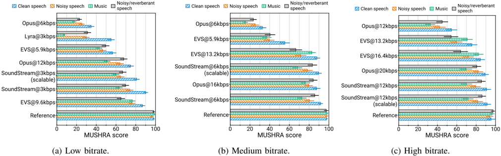Figure 6 illustrates the results of the subjective evaluation by content type. We observe that the quality of SoundStream remains consistent when encoding clean speech and noisy speech. In addition, SoundStream can encode music when using as little as 3 kbps, with quality significantly better than Opus at 12 kbps and EVS at 5.9 kbps. This is the first time that a codec is shown to operate on diverse content types at such a low bitrate. ## B. 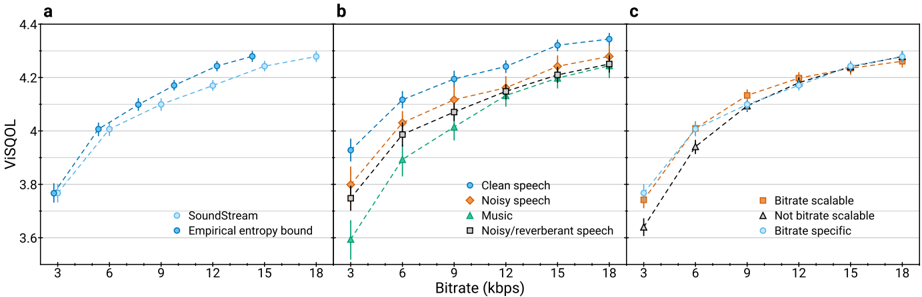Objective quality metrics Figure 7a shows the rate-quality curve of SoundStream over a wide range of bitrates, from 3 kbps to 18 kbps. We observe that quality, as measured by means of ViSQOL, gracefully decreases as the bitrate is reduced and it remains above 3.7 even at the lowest bitrate. In our work, SoundStream operates at constant bitrate, i.e., the same number of bits is allocated to each encoded frame. At the same time, we measure the bitrate lower bound by computing the empirical entropy of the quantization symbols of the vector quantizers, assuming each vector quantizer to be a discrete memoryless source, i.e., no statistical redundancy is exploited across different layers of the residual vector quantizer, nor across time. Figure 7a indicates a potential rate saving between 7% and 20%. We also investigate the rate-quality tradeoff achieved when encoding different content types, as illustrated in Figure 7b. Unsurprisingly, the highest quality is achieved when encoding clean speech. Music represents a more challenging case, due to its inherent diversity of content. 1 https://google-research.github.io/seanet/soundstream/examples/ Fig. 5: Subjective evaluation results. Error bars denote 95% confidence intervals. <details> <summary>Image 6 Details</summary>  ### Visual Description ## Scatter Plots: MUSHRA Scores vs. Bitrate Across Three Bitrate Ranges ### Overview The image contains three scatter plots comparing audio codec performance (MUSHRA scores) across low, medium, and high bitrate ranges. Each plot uses bitrate (kbps) on the x-axis and MUSHRA scores (0-100) on the y-axis. Five codecs are compared: SoundStream, SoundStream - scalable, EVS, Opus, and Lyra. ### Components/Axes - **X-axis (Bitrate)**: - (a) Low bitrate: 3–12 kbps - (b) Medium bitrate: 6–15 kbps - (c) High bitrate: 12–21 kbps - **Y-axis (MUSHRA Score)**: 20–80 across all plots - **Legend**: - SoundStream: Blue diamond - SoundStream - scalable: Blue circle - EVS: Green diamond - Opus: Orange star - Lyra: Gray triangle ### Detailed Analysis #### (a) Low Bitrate (3–12 kbps) - **SoundStream**: 6 kbps, ~70 score (blue diamond) - **SoundStream - scalable**: 6 kbps, ~65 score (blue circle) - **EVS**: 6 kbps, ~50 score (green diamond) - **Opus**: 12 kbps, ~60 score (orange star) - **Lyra**: 3 kbps, ~30 score (gray triangle) #### (b) Medium Bitrate (6–15 kbps) - **SoundStream**: 9 kbps, ~80 score (blue diamond) - **SoundStream - scalable**: 9 kbps, ~75 score (blue circle) - **EVS**: 9 kbps, ~45 score (green diamond) - **Opus**: 15 kbps, ~80 score (orange star) #### (c) High Bitrate (12–21 kbps) - **SoundStream**: 12 kbps, ~85 score (blue diamond) - **SoundStream - scalable**: 12 kbps, ~80 score (blue circle) - **EVS**: 15 kbps, ~70 score (green diamond) - **Opus**: 21 kbps, ~80 score (orange star) ### Key Observations 1. **SoundStream** consistently achieves the highest scores across all bitrates, with a notable peak at 85 in high bitrate. 2. **Opus** performs strongly at higher bitrates (80 in medium/high) but lags behind SoundStream in low bitrate. 3. **EVS** shows the lowest scores in low/medium bitrates (~45–50) but improves to ~70 in high bitrate. 4. **SoundStream - scalable** underperforms its non-scalable counterpart in low/medium bitrates but matches it in high bitrate. 5. **Lyra** is only tested at 3 kbps with the lowest score (~30), suggesting poor performance at ultra-low bitrates. ### Interpretation - **Efficiency Trends**: SoundStream and Opus demonstrate superior efficiency, maintaining high scores even at lower bitrates. EVS requires higher bitrates to achieve competitive performance. - **Scalability Impact**: The scalable version of SoundStream loses ~5 points in low/medium bitrates but converges with the non-scalable version at high bitrates, suggesting scalability trade-offs at lower bitrates. - **Lyra's Outlier**: Lyra's inclusion only in low bitrate with a score of ~30 highlights its unsuitability for higher-quality applications, even at minimal compression. - **Bitrate-Quality Relationship**: Higher bitrates generally improve MUSHRA scores, but codec choice significantly influences outcomes. SoundStream and Opus outperform others across the spectrum, while EVS and Lyra require higher bitrates to compete. This analysis underscores the importance of codec selection based on bitrate constraints and quality requirements. SoundStream emerges as the most robust performer, while EVS and Lyra show context-dependent limitations. </details> Fig. 6: Subjective evaluation results by content type. Error bars denote 95% confidence intervals. <details> <summary>Image 7 Details</summary>  ### Visual Description ## Bar Charts: MUSHRA Scores for Audio Codecs AcrossBitrates ### Overview The image contains three side-by-side bar charts comparing MUSHRA (Multidimensional Speech Quality Evaluation) scores for audio codecs under three bitrate categories: **Low**, **Medium**, and **High**. Each chart evaluates four conditions: **Clean speech**, **Noisy speech**, **Music**, and **Noisy/reverberant speech**. The y-axis lists codecs (e.g., Opus, ESVs, SoundStream) with their bitrates, while the x-axis represents scores from 0 to 100. The **Reference** codec consistently achieves the highest scores across all conditions and bitrates. ### Components/Axes - **X-axis**: MUSHRA score (0–100), labeled "MUSHRA score". - **Y-axis**: Audio codecs and bitrates (e.g., "Opus@6kbps", "SoundStream@3kbps (scalable)"). - **Legend**: Located on the left, with four categories: - **Clean speech** (blue, solid bars) - **Noisy speech** (orange, dashed bars) - **Music** (green, dotted bars) - **Noisy/reverberant speech** (gray, striped bars) - **Charts**: Three horizontal bar charts labeled **(a) Low bitrate**, **(b) Medium bitrate**, **(c) High bitrate**. ### Detailed Analysis #### Low Bitrate (a) - **Opus@6kbps**: Clean (~30), Noisy (~25), Music (~20), Noisy/reverberant (~15). - **Lyra@3kbps**: Clean (~40), Noisy (~35), Music (~30), Noisy/reverberant (~25). - **EVS@5.9kbps**: Clean (~50), Noisy (~45), Music (~40), Noisy/reverberant (~35). - **SoundStream@3kbps (scalable)**: Clean (~60), Noisy (~55), Music (~50), Noisy/reverberant (~45). - **Reference**: All conditions ~90. #### Medium Bitrate (b) - **Opus@6kbps**: Clean (~40), Noisy (~35), Music (~30), Noisy/reverberant (~25). - **EVS@5.9kbps**: Clean (~50), Noisy (~45), Music (~40), Noisy/reverberant (~35). - **EVS@13.2kbps**: Clean (~70), Noisy (~60), Music (~55), Noisy/reverberant (~50). - **SoundStream@6kbps (scalable)**: Clean (~80), Noisy (~75), Music (~70), Noisy/reverberant (~65). - **Opus@16kbps**: Clean (~85), Noisy (~78), Music (~72), Noisy/reverberant (~68). - **Reference**: All conditions ~95. #### High Bitrate (c) - **Opus@12kbps**: Clean (~50), Noisy (~45), Music (~40), Noisy/reverberant (~35). - **EVS@13.2kbps**: Clean (~70), Noisy (~60), Music (~55), Noisy/reverberant (~50). - **EVS@16.4kbps**: Clean (~80), Noisy (~75), Music (~70), Noisy/reverberant (~65). - **Opus@20kbps**: Clean (~85), Noisy (~78), Music (~72), Noisy/reverberant (~68). - **SoundStream@12kbps (scalable)**: Clean (~90), Noisy (~85), Music (~80), Noisy/reverberant (~75). - **Reference**: All conditions ~98. ### Key Observations 1. **Reference Codec Dominance**: The Reference codec consistently achieves the highest scores (~90–98) across all bitrates and conditions, serving as the benchmark. 2. **Bitrate Impact**: Higher bitrates improve performance for all codecs, but the gap between codecs narrows at higher bitrates (e.g., SoundStream@12kbps in High bitrate approaches Reference scores). 3. **Noisy/Reverberant Speech**: All codecs perform worst under noisy/reverberant conditions, with scores 10–20 points lower than Clean speech. 4. **SoundStream Scalability**: SoundStream (scalable) shows strong performance in Medium and High bitrates, often outperforming fixed-bitrate codecs like Opus. 5. **EVS Performance**: EVS improves with higher bitrates (e.g., EVS@16.4kbps in High bitrate scores ~80 for Clean speech). ### Interpretation The data demonstrates that **bitrate significantly influences codec performance**, with higher bitrates enabling better fidelity. The **Reference codec** remains the gold standard, but scalable codecs like **SoundStream** adapt effectively to higher bitrates, closing performance gaps. Noisy/reverberant conditions universally degrade scores, highlighting challenges in real-world environments. The results suggest that **codec efficiency and adaptability** (e.g., SoundStream’s scalability) are critical for applications requiring robust performance across varying network conditions. </details> ## C. Bitrate scalability We investigate the bitrate scalability provided by training a single model that can serve different bitrates. To evaluate this aspect, for each bitrate R we consider three SoundStream configurations: a) a non-scalable model trained and evaluated at bitrate R ( bitrate specific ); b) a non-scalable model trained at 18kbps and evaluated at bitrate R by using only the first n q quantizers during inference ( 18 kbps - no dropout ); c) a scalable model trained with quantizer dropout and evaluated at bitrate R ( bitrate scalable ). Figure 7c shows the ViSQOL scores for these three scenarios. Remarkably, a model trained specifically at 18 kbps retains good performance when evaluated at lower bitrates, even though the model was not trained in these conditions. Unsurprisingly, the quality drop increases as the bitrate decreases, i.e., when there is a more significant difference between training and inference. This gap vanishes when using the quantizer dropout strategy described in Section III-C. Surprisingly, the bitrate scalable model seems to marginally outperform bitrate specific models at 9 kbps and 12 kbps. This suggests that quantizer dropout, beyond providing bitrate scalability, may act as a regularizer. We confirm these results by including the bitrate scalable variant of SoundStream in the MUSHRA subjective evaluation (see Figure 5). When operating at 3 kbps, the bitrate scalable variant of SoundStream is only slightly worse than the bitrate specific variant. Conversely, both at 6 kbps and 12 kbps it matches the same quality as the bitrate specific variant. ## D. Ablation studies We carried out several additional experiments to evaluate the impact of some of the design choices applied to SoundStream . Unless stated otherwise, all these experiments operate at 6 kbps. Advantage of learning the encoder - We explored the impact of replacing the learnable encoder of SoundStream with a fixed mel-filterbank, similarly to Lyra [8]. We learned both the quantizer and the decoder and observed a significant drop in objective quality, with ViSQOL going from 3.96 to 3.33. Note that this is significantly worse than what can be achieved when learning the encoder and halving the bitrate (i.e., ViSQOL equal to 3.76 at 3 kbps). This demonstrates that the additional complexity of having a learnable encoder translates to a very significant improvement in the rate-quality trade-off. Encoder and decoder capacity - The main drawback of using a learnable encoder is the computational cost of the neural architecture, which can be significantly higher than computing fixed, non-learnable features such as mel-filterbanks. Fig. 7: ViSQOL vs. bitrate. a) SoundStream performance on test data, comparing the actual bitrate with the potential bitrate savings achievable by entropy coding b) ViSQOL scores by content type c) Comparison of SoundStream models that are trained at 18 kbps with quantizer dropout (bitrate scalable), without quantizer dropout (not bitrate scalable) and evaluated with a variable number of quantizers, or trained and evaluated at a fixed bitrate (bitrate specific). Error bars denote 95% confidence intervals. <details> <summary>Image 8 Details</summary>  ### Visual Description ## Line Graphs: ViSQOL vs. Bitrate Across Different Conditions ### Overview The image contains three subplots (a, b, c) comparing ViSQOL scores against bitrate (3–18 kbps) for various audio conditions. Each subplot uses distinct data series and legends to represent different scenarios. --- ### Components/Axes - **X-axis**: Bitrate (kbps), ranging from 3 to 18 kbps in increments of 3. - **Y-axis**: ViSQOL score, ranging from 3.6 to 4.4. - **Legends**: - **Subplot a**: - Dashed blue line with circles: **SoundStream** - Solid blue line with diamonds: **Empirical entropy bound** - **Subplot b**: - Blue circles: **Clean speech** - Orange diamonds: **Noisy speech** - Green triangles: **Music** - Black squares: **Noisy/reverberant speech** - **Subplot c**: - Orange diamonds: **Bitrate scalable** - Black triangles: **Not bitrate scalable** - Blue circles: **Bitrate specific** --- ### Detailed Analysis #### Subplot a - **Trend**: Both lines show a consistent upward trend. The dashed line (SoundStream) starts slightly below the solid line (Empirical entropy bound) but converges near 18 kbps. - **Data Points**: - At 3 kbps: SoundStream ≈ 3.78, Empirical entropy bound ≈ 3.78. - At 18 kbps: SoundStream ≈ 4.28, Empirical entropy bound ≈ 4.30. #### Subplot b - **Trend**: All series increase with bitrate, but starting points and growth rates vary. - **Clean speech**: Steady rise from ~3.9 to ~4.3. - **Noisy speech**: Starts lower (~3.8) but grows to ~4.2. - **Music**: Starts lowest (~3.6) but rises steeply to ~4.1. - **Noisy/reverberant speech**: Moderate growth from ~3.7 to ~4.2. - **Data Points**: - At 3 kbps: Clean speech ≈ 3.9, Noisy speech ≈ 3.8, Music ≈ 3.6, Noisy/reverberant ≈ 3.7. - At 18 kbps: Clean speech ≈ 4.35, Noisy speech ≈ 4.25, Music ≈ 4.15, Noisy/reverberant ≈ 4.2. #### Subplot c - **Trend**: All series increase, but "Bitrate scalable" and "Bitrate specific" outperform "Not bitrate scalable." - **Bitrate scalable**: Starts at ~3.8, ends at ~4.3. - **Not bitrate scalable**: Starts at ~3.7, ends at ~4.2. - **Bitrate specific**: Starts at ~3.9, ends at ~4.3. - **Data Points**: - At 3 kbps: Bitrate scalable ≈ 3.8, Not bitrate scalable ≈ 3.7, Bitrate specific ≈ 3.9. - At 18 kbps: Bitrate scalable ≈ 4.28, Not bitrate scalable ≈ 4.2, Bitrate specific ≈ 4.3. --- ### Key Observations 1. **Bitrate Correlation**: Higher bitrates consistently improve ViSQOL scores across all conditions. 2. **Content Type Impact**: Music (subplot b) shows the lowest initial ViSQOL but gains significantly with bitrate, suggesting sensitivity to compression artifacts. 3. **Scalability**: "Bitrate scalable" (subplot c) outperforms "Not bitrate scalable," indicating adaptive bitrate strategies enhance quality. 4. **Empirical Bound**: In subplot a, the "Empirical entropy bound" closely tracks the "SoundStream" line, suggesting it represents a theoretical upper limit for ViSQOL. --- ### Interpretation The data demonstrates that **bitrate is a critical factor in audio quality**, with higher bitrates improving ViSQOL scores across diverse conditions. However, the **type of content** (e.g., music vs. speech) and **bitrate scalability** significantly influence performance. For instance: - **Music** requires higher bitrates to achieve parity with speech, likely due to its complex frequency content. - **Bitrate scalable** methods (subplot c) outperform fixed or non-scalable approaches, highlighting the value of adaptive bitrate allocation. - The **Empirical entropy bound** in subplot a suggests a theoretical ceiling for ViSQOL, which practical systems like SoundStream approach but do not exceed. These findings underscore the importance of optimizing bitrate allocation based on content type and system capabilities to maximize perceived audio quality. </details> TABLE I: Audio quality (ViSQOL) and model complexity (number of parameters and real-time factor) for different capacity trade-offs between encoder and decoder, at 6kbps. | C enc | C dec | #Params | RTF (enc) | RTF (dec) | ViSQOL | |-----------------|-----------------|-----------------|-----------------|-----------------|-----------------| | 32 | 32 | 8 . 4M | 2.4 × | 2.3 × | 4.01 ± 0.03 | | 16 | 16 | 2 . 4M | 7.5 × | 7.1 × | 3.98 ± 0.03 | | Smaller encoder | Smaller encoder | Smaller encoder | Smaller encoder | Smaller encoder | Smaller encoder | | 16 | 32 | 5 . 5M | 7.5 × | 2.3 × | 4.02 ± 0.03 | | 8 | 32 | 4 . 8M | 18.6 × | 2.3 × | 3.99 ± 0.03 | | Smaller decoder | Smaller decoder | Smaller decoder | Smaller decoder | Smaller decoder | Smaller decoder | | 32 | 16 | 5 . 3M | 2.4 × | 7.1 × | 3.97 ± 0.03 | | 32 | 8 | 4 . 4M | 2.4 × | 17.1 × | 3.90 ± 0.03 | For SoundStream to be competitive with traditional codecs, not only should it provide a better perceptual quality at an equivalent bitrate, but it must also run in real-time on resourcelimited hardware. Table I shows how computational efficiency and audio quality are impacted by the number of channels in the encoder C enc and the decoder C dec. We measured the real-time factor (RTF), defined as the ratio between the temporal length of the input audio and the time needed for encoding/decoding it with SoundStream . We profiled these models on a single CPU thread of a Pixel4 smartphone. We observe that the default model ( C enc = C dec = 32 ) runs in real-time (RTF > 2 . 3 × ). Decreasing the model capacity by setting C enc = C dec = 16 only marginally affects the reconstruction quality while increasing the real-time factor significantly (RTF > 7 . 1 × ). We also investigated configurations with asymmetric model capacities. Using a smaller encoder, it is possible to achieve a significant speedup without sacrificing quality (ViSQOL drops from 3.96 to 3.94, while the encoder RTF increases to 18 . 6 × ). Instead, decreasing the capacity of the decoder has a more significant impact on quality (ViSQOL drops from 3.96 to 3.84). This is aligned with recent findings in the field of neural image compression [61], which also adopt a lighter encoder and a heavier decoder. Vector quantizer depth and codebook size - The number of bits used to encode a single frame is equal to N q log 2 N , where TABLE II: Trade-off between residual vector quantizer depth and codebook size at 6 kbps. | Number of quantizers N q Codebook size N | 8 1024 | 16 32 | 80 2 | |--------------------------------------------|----------|---------|--------| TABLE III: Audio quality (ViSQOL) and real-time factor for different levels of architectural latency, defined by the total striding factor of the encoder/decoder, at 6 kbps. | Strides | Latency | N q | RTF (enc) | RTF (dec) | ViSQOL | |-----------------|-----------|-------|-------------|-------------|-------------| | (1 , 4 , 5 , 8) | 7.5 ms | 4 | 1.6 × | 1.5 × | 4.01 ± 0.02 | | (2 , 4 , 5 , 8) | 13 ms | 8 | 2.4 × | 2.3 × | 4.01 ± 0.03 | | (4 , 4 , 5 , 8) | 26 ms | 16 | 4.1 × | 4.0 × | 4.01 ± 0.03 | N q denotes the number of quantizers and N the codebook size. Hence, it is possible to achieve the same target bitrate for different combinations of N q and N . Table II shows three configurations, all operating at 6 kbps. As expected, using fewer vector quantizers, each with a larger codebook, achieves the highest coding efficiency at the cost of higher computational complexity. Remarkably, using a sequence of 80 1-bit quantizers leads only to a modest quality degradation. This demonstrates that it is possible to successfully train very deep residual vector quantizers without facing optimization issues. On the other side, as discussed in Section III-C, growing the codebook size can quickly lead to unmanageable memory requirements. Thus, the proposed residual vector quantizer offers a practical and effective solution for learning neural codecs operating at high bitrates, as it scales gracefully when using many quantizers, each with a smaller codebook. Latency - The architectural latency M of the model is defined by the product of the strides, as explained in Section III-A. In our default configuration, M = 2 · 4 · 5 · 8 = 320 samples, which means that one frame corresponds to 13.3 ms of audio at 24 kHz. The bit budget allocated to the residual vector quantizer needs to be adjusted based on the target architectural latency. 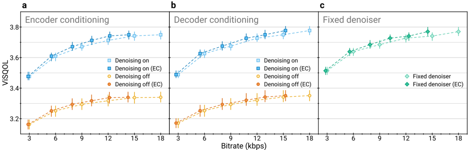For example, when operating at 6 kbps, the residual Fig. 8: Performance of SoundStream when performing joint compression and background noise suppression, measured by ViSQOL scores at different bitrates. We compare three variants: a) flexible denoising, where the conditioning is added at the encoder side; b) flexible denoising, where the conditioning is added at the decoder side; and c) fixed denoising, where the model was trained to always produce clean outputs. For all models we also report the potential bitrate savings achievable by entropy coding (EC). Error bars denote 95% confidence intervals. <details> <summary>Image 9 Details</summary>  ### Visual Description ## Line Graphs: ViSQOL vs. Bitrate under Different Conditioning Strategies ### Overview The image contains three line graphs (a, b, c) comparing ViSQOL (a perceptual video quality metric) against bitrate (kbps) under three distinct denoising configurations: - **a) Encoder conditioning** - **b) Decoder conditioning** - **c) Fixed denoiser** Each graph includes two data series: 1. **Denoising on** (solid markers) 2. **Denoising off** (hollow markers) With subcategories for **EC (Error Correction)** and non-EC variants. --- ### Components/Axes - **X-axis**: Bitrate (kbps), ranging from 3 to 18. - **Y-axis**: ViSQOL score, ranging from 3.2 to 3.8. - **Legends**: - **Top-right** of each subplot. - **Colors/markers**: - **Blue squares**: Denoising on (non-EC). - **Blue diamonds**: Denoising on (EC). - **Orange circles**: Denoising off (non-EC). - **Orange triangles**: Denoising off (EC). - **Green diamonds**: Fixed denoiser (EC). - **Green squares**: Fixed denoiser (non-EC). --- ### Detailed Analysis #### Graph a: Encoder Conditioning - **Denoising on (blue squares)**: - Starts at ~3.5 ViSQOL at 3 kbps. - Increases steadily to ~3.75 at 18 kbps. - Slope: ~0.015 ViSQOL per kbps. - **Denoising off (orange circles)**: - Starts at ~3.2 ViSQOL at 3 kbps. - Increases slowly to ~3.35 at 18 kbps. - Slope: ~0.003 ViSQOL per kbps. - **EC variants**: - Denoising on (blue diamonds) and off (orange triangles) show marginally higher ViSQOL (~0.05–0.1 improvement) than non-EC. #### Graph b: Decoder Conditioning - **Denoising on (blue squares)**: - Starts at ~3.5 ViSQOL at 3 kbps. - Rises to ~3.75 at 18 kbps. - Slope: ~0.015 ViSQOL per kbps. - **Denoising off (orange circles)**: - Starts at ~3.2 ViSQOL at 3 kbps. - Increases to ~3.35 at 18 kbps. - Slope: ~0.003 ViSQOL per kbps. - **EC variants**: - Similar to graph a, with minor EC improvements. #### Graph c: Fixed Denoiser - **Fixed denoiser (green squares)**: - Starts at ~3.5 ViSQOL at 3 kbps. - Increases to ~3.75 at 18 kbps. - Slope: ~0.015 ViSQOL per kbps. - **Fixed denoiser (EC) (green diamonds)**: - Slightly higher ViSQOL (~3.6–3.75) than non-EC. --- ### Key Observations 1. **Denoising improves ViSQOL**: - Across all graphs, denoising on (solid markers) consistently outperforms denoising off (hollow markers). - Example: At 18 kbps, denoising on achieves ~3.75 ViSQOL vs. ~3.35 for denoising off. 2. **EC enhances performance**: - EC variants (dashed lines) show small but consistent gains (~0.05–0.1 ViSQOL) over non-EC. 3. **Fixed denoiser efficacy**: - In graph c, the fixed denoiser matches the performance of encoder/decoder conditioning, suggesting static models can achieve comparable results. 4. **Bitrate dependency**: - ViSQOL improvements plateau at higher bitrates (~15–18 kbps), indicating diminishing returns. --- ### Interpretation - **Technical Implications**: - Denoising significantly boosts perceptual quality, with encoder/decoder conditioning offering similar gains. - EC (e.g., error correction) provides marginal but measurable improvements, suggesting robustness to noise. - Fixed denoisers are viable alternatives to dynamic conditioning, potentially reducing computational overhead. - **Trade-offs**: - Higher bitrates yield diminishing returns, implying efficient bitrate allocation strategies. - EC mechanisms may add complexity but improve reliability in noisy environments. - **Anomalies**: - No outliers observed; all trends align with expected bitrate-quality relationships. This analysis underscores the importance of denoising in video quality optimization, with encoder/decoder conditioning and EC offering complementary benefits. </details> vector quantizer has a budget of 80 bits per frame. If we double the latency, one frame corresponds to 26.6 ms , so the per-frame budget needs to be increased to 160 bits. Table III compares three configurations, all operating at 6 kbps, where the budget is adjusted by changing the number of quantizers, while keeping the codebook size fixed. We observe that these three configurations are equivalent in terms of audio quality. At the same time, increasing the latency of the model significantly increases the real-time factor, as encoding/decoding of a single frame corresponds to a longer audio sample. ## E. Joint compression and enhancement We evaluate a variant of SoundStream that is able to jointly perform compression and background noise suppression, which was trained as described in Section III-F. We consider two configurations, in which the conditioning signal is applied to the embeddings: i) one where the conditioning signal is added at the encoder side, just before quantization; ii) another where it is added at the decoder side. For each configuration, we train models at different bitrates. For evaluation we use 1000 samples of noisy speech, generated as described in Section IV-A and compute ViSQOL scores when denoising is enabled or disabled, using clean speech references as targets. Figures 8 shows a substantial improvement of quality when denoising is enabled, with no significant difference between denoising either at the encoder or at the decoder. We observe that the proposed model, which is able to flexibly enable or disable denoising at inference time, does not incur a cost in performance, when compared with a model in which denoising is always enabled. This can be seen comparing Figure 8c with Figure 8a and Figure 8b. We also investigate whether denoising affects the potential bitrate savings that would be achievable by entropy coding. To evaluate this aspect, we first measured the empirical probability distributions p ( q ) i , i = 1 . . . N, q = 1 . . . N q on 3200 samples of training data. Then, we measured the empirical distribution r ( q ) i on the 1000 test samples and computed the cross-entropy H ( r, p ) = -∑ i,q r ( q ) i log 2 p ( q ) i , as an estimate of the bitrate lower bound needed to encode the test samples. Figure 8 shows that both the encoder-side denoising and fixed denoising offer substantial bitrate savings when compared with decoder-side denoising. Hence, applying denoising before quantization leads to a representation that can be encoded with fewer bits. ## F. Joint vs. disjoint compression and enhancement We compare the proposed model, which is able to perform joint compression and enhancement, with a configuration in which compression is performed by SoundStream (with denoising disabled) and enhancement by a dedicated denoising model. For the latter, we adopt SEANet [45], which features a very similar model architecture, with the notable exception of skip connections between encoder and decoder layers and the absence of quantization. We consider two variants: i) one in which compression is followed by denoising (i.e., denoising is applied at the decoder side); ii) another one in which denoising is followed by compression (i.e., denoising is applied at the encoder side). We evaluate the different models using the VCTK dataset [62], which was neither used for training SoundStream nor SEANet. The input samples are 2 s clips of noisy speech cropped to reduce periods of silence and resampled at 24 kHz. For each of the four input signal-to-noise ratios ( 0 dB, 5 dB, 10 dB and 15 dB), we run inference on 1000 samples and compute ViSQOL scores. As shown in Table IV, one single model trained for joint compression and enhancement achieves a level of quality that is almost on par with using two disjoint models. Also, the former requires only half of the computational cost and incurs no additional architectural latency, which would be introduced when stacking disjoint models. We also observe that the performance gap decreases as the input SNR increases. ## VI. CONCLUSIONS We propose SoundStream , a novel neural audio codec that outperforms state-of-the-art audio codecs over a wide range of bitrates and content types. SoundStream consists of an TABLE IV: Comparison of SoundStream as a joint denoiser and codec with SEANet as a denoiser compressed by a SoundStream codec at different signal-to-noise ratios. Uncertainties denote 95% confidence intervals. | | ViSQOL | ViSQOL | ViSQOL | |-----------|-------------|----------------------|----------------------| | Input SNR | SoundStream | SoundStream → SEANet | SEANet → SoundStream | | 0 dB | 2.93 ± 0.02 | 3.02 ± 0.03 | 3.05 ± 0.02 | | 5 dB | 3.18 ± 0.02 | 3.30 ± 0.02 | 3.31 ± 0.02 | | 10 dB | 3.42 ± 0.02 | 3.51 ± 0.02 | 3.50 ± 0.02 | | 15 dB | 3.58 ± 0.02 | 3.64 ± 0.02 | 3.63 ± 0.02 | encoder, a residual vector quantizer and a decoder, which are trained end-to-end using a mix of adversarial and reconstruction losses to achieve superior audio quality. The model supports streamable inference and can run in real-time on a single smartphone CPU. When trained with quantizer dropout, a single SoundStream model achieves bitrate scalability with a minimal loss in performance when compared with bitratespecific models. In addition, we show that it is possible to combine compression and enhancement in a single model without introducing additional latency. ## ACKNOWLEDGMENTS The authors thank Yunpeng Li, Dominik Roblek, F´ elix de Chaumont Quitry and Dick Lyon for their feedback on this work. ## REFERENCES - [1] Y. Li, M. Tagliasacchi, O. Rybakov, V. Ungureanu, and D. Roblek, 'Real-time speech frequency bandwidth extension,' in IEEE International Conference on Acoustics, Speech and Signal Processing (ICASSP) , 2021, pp. 691-695. - [2] A. Biswas and D. Jia, 'Audio codec enhancement with generative adversarial networks,' in IEEE International Conference on Acoustics, Speech and Signal Processing (ICASSP) , 2020, pp. 356-360. - [3] F. Stimberg, A. Narest, A. Bazzica, L. Kolmodin, P. Barrera Gonz´ alez, O. Sharonova, H. Lundin, and T. C. Walters, 'WaveNetEQ - Packet loss concealment with WaveRNN,' in 54th Asilomar Conference on Signals, Systems, and Computers , 2020, pp. 672-676. - [4] A. van den Oord, S. Dieleman, H. Zen, K. Simonyan, O. Vinyals, A. Graves, N. Kalchbrenner, A. Senior, and K. Kavukcuoglu, 'WaveNet: A generative model for raw audio,' arXiv:1609.03499 , 2016. - [5] W. B. Kleijn, F. S. Lim, A. Luebs, J. Skoglund, F. Stimberg, Q. Wang, and T. C. Walters, 'Wavenet based low rate speech coding,' in IEEE international conference on acoustics, speech and signal processing (ICASSP) , 2018, pp. 676-680. - [6] C. Gˆ arbacea, A. van den Oord, Y. Li, F. S. C. Lim, A. Luebs, O. Vinyals, and T. C. Walters, 'Low bit-rate speech coding with VQ-VAE and a WaveNet decoder,' in IEEE International Conference on Acoustics, Speech and Signal Processing (ICASSP) , 2019, pp. 735-739. - [7] J.-M. Valin and J. Skoglund, 'LPCNet: improving neural speech synthesis through linear prediction,' in IEEE International Conference on Acoustics, Speech and Signal Processing (ICASSP) , 2019, pp. 5891-5895. - [8] W. B. Kleijn, A. Storus, M. Chinen, T. Denton, F. S. C. Lim, A. Luebs, J. Skoglund, and H. Yeh, 'Generative speech coding with predictive variance regularization,' arXiv:2102.09660 , 2021. - [9] J.-M. Valin, K. Vos, and T. B. Terriberry, 'Definition of the Opus Audio Codec,' IETF RFC 6716, 2012, https://tools.ietf.org/html/rfc6716 . - [10] M. Dietz, M. Multrus, V. Eksler, V. Malenovsky, E. Norvell, H. Pobloth, L. Miao, Z. Wang, L. Laaksonen, A. Vasilache, Y. Kamamoto, K. Kikuiri, S. Ragot, J. Faure, H. Ehara, V. Rajendran, V. Atti, H. Sung, E. Oh, H. Yuan, and C. Zhu, 'Overview of the EVS codec architecture,' in IEEE International Conference on Acoustics, Speech and Signal Processing (ICASSP) , 2015, pp. 5698-5702. - [11] S. Mehri, K. Kumar, I. Gulrajani, R. Kumar, S. Jain, J. Sotelo, A. Courville, and Y. Bengio, 'SampleRNN: An unconditional end-to-end neural audio generation model,' arXiv:1612.07837 , 2017. - [12] A. van den Oord, Y. Li, I. Babuschkin, K. Simonyan, O. Vinyals, K. Kavukcuoglu, G. van den Driessche, E. Lockhart, L. Cobo, F. Stimberg, N. Casagrande, D. Grewe, S. Noury, S. Dieleman, E. Elsen, N. Kalchbrenner, H. Zen, A. Graves, H. King, T. Walters, D. Belov, and D. Hassabis, 'Parallel WaveNet: Fast high-fidelity speech synthesis,' in Proceedings of the 35th International Conference on Machine Learning , 2018, pp. 3918-3926. - [13] N. Kalchbrenner, E. Elsen, K. Simonyan, S. Noury, N. Casagrande, E. Lockhart, F. Stimberg, A. van den Oord, S. Dieleman, and K. Kavukcuoglu, 'Efficient neural audio synthesis,' arXiv:1802.08435 , 2018. - [14] Z. Jin, A. Finkelstein, G. J. Mysore, and J. Lu, 'FFTNet: a real-time speaker-dependent neural vocoder,' in IEEE International Conference on Acoustics, Speech and Signal Processing (ICASSP) , 2018, pp. 2251-2255. - [15] K. Kumar, R. Kumar, T. de Boissiere, L. Gestin, W. Z. Teoh, J. Sotelo, A. de Brebisson, Y. Bengio, and A. Courville, 'MelGAN: Generative adversarial networks for conditional waveform synthesis,' in Advances in Neural Information Processing Systems , 2019. - [16] J. Kong, J. Kim, and J. Bae, 'HiFi-GAN: Generative Adversarial Networks for efficient and high fidelity speech synthesis,' arXiv:2010.05646 , 2020. - [17] X. Feng, Y. Zhang, and J. Glass, 'Speech feature denoising and dereverberation via deep autoencoders for noisy reverberant speech recognition,' in IEEE International Conference on Acoustics, Speech and Signal Processing (ICASSP) , 2014, pp. 1759-1763. - [18] S. Pascual, A. Bonafonte, and J. Serra, 'SEGAN: Speech enhancement generative adversarial network,' arXiv:1703.09452 , 2017. - [19] F. G. Germain, Q. Chen, and V. Koltun, 'Speech denoising with deep feature losses,' arXiv:1806.10522 , 2018. - [20] D. Rethage, J. Pons, and X. Serra, 'A WaveNet for speech denoising,' in IEEE International Conference on Acoustics, Speech and Signal Processing (ICASSP) , 2018, pp. 5069-5073. - [21] C. Donahue, B. Li, and R. Prabhavalkar, 'Exploring speech enhancement with generative adversarial networks for robust speech recognition,' in 2018 IEEE International Conference on Acoustics, Speech and Signal Processing (ICASSP) , 2018, pp. 5024-5028. - [22] T. Ishii, H. Komiyama, T. Shinozaki, Y. Horiuchi, and S. Kuroiwa, 'Reverberant speech recognition based on denoising autoencoder.' in Interspeech , 2013, pp. 3512-3516. - [23] D. S. Williamson and D. Wang, 'Time-frequency masking in the complex domain for speech dereverberation and denoising,' IEEE/ACM Transactions on Audio, Speech, and Language Processing , vol. 25, pp. 1492-1501, 2017. - [24] T. Y. Lim, R. A. Yeh, Y. Xu, M. N. Do, and M. Hasegawa-Johnson, 'Timefrequency networks for audio super-resolution,' in IEEE International Conference on Acoustics, Speech and Signal Processing (ICASSP) , 2018, pp. 646-650. - [25] S. Lloyd, 'Least squares quantization in PCM,' IEEE transactions on information theory , vol. 28, pp. 129-137, 1982. - [26] Y. Linde, A. Buzo, and R. Gray, 'An algorithm for vector quantizer design,' IEEE Transactions on Communications , vol. 28, pp. 84-95, 1980. - [27] J. MacQueen, 'Some methods for classification and analysis of multivariate observations,' Proceedings of the Fifth Berkeley Symposium on Mathematical Statistics and Probability , pp. 281-297, 1967. - [28] R. Gray, 'Vector quantization,' IEEE ASSP Magazine , vol. 1, pp. 4-29, 1984. - [29] J. Makhoul, S. Roucos, and H. Gish, 'Vector quantization in speech coding,' Proceedings of the IEEE , vol. 73, pp. 1551-1588, 1985. - [30] M. Schroeder and B. Atal, 'Code-excited linear prediction (CELP): Highquality speech at very low bit rates,' in IEEE International Conference on Acoustics, Speech, and Signal Processing (ICASSP) , 1985, pp. 937-940. - [31] A. van den Oord, O. Vinyals, and K. Kavukcuoglu, 'Neural discrete representation learning,' arXiv:1711.00937 , 2017. - [32] A. Razavi, A. van den Oord, and O. Vinyals, 'Generating diverse highfidelity images with VQ-VAE-2,' arXiv:1906.00446 , 2019. - [33] S. Dieleman, A. van den Oord, and K. Simonyan, 'The challenge of realistic music generation: Modelling raw audio at scale,' arXiv:1806.10474 , 2018. - [34] P. Dhariwal, H. Jun, C. Payne, J. W. Kim, A. Radford, and I. Sutskever, 'Jukebox: A generative model for music,' arXiv:2005.00341 , 2020. - [35] B.-H. Juang and A. Gray, 'Multiple stage vector quantization for speech coding,' in IEEE International Conference on Acoustics, Speech, and Signal Processing (ICASSP) , 1982, pp. 597-600. - [36] A. Vasuki and P. Vanathi, 'A review of vector quantization techniques,' IEEE Potentials , vol. 25, pp. 39-47, 2006. - [37] S. Morishima, H. Harashima, and Y. Katayama, 'Speech coding based on a multi-layer neural network,' in IEEE International Conference on Communications, Including Supercomm Technical Sessions , 1990, pp. 429-433. - [38] S. Kankanahalli, 'End-to-end optimized speech coding with deep neural networks,' in IEEE International Conference on Acoustics, Speech and Signal Processing (ICASSP) , 2018, pp. 2521-2525. - [39] A. Polyak, Y. Adi, J. Copet, E. Kharitonov, K. Lakhotia, W.-N. Hsu, A. Mohamed, and E. Dupoux, 'Speech resynthesis from discrete disentangled self-supervised representations,' arXiv:2104.00355 , 2021. - [40] K. Zhen, J. Sung, M. S. Lee, S. Beack, and M. Kim, 'Cascaded crossmodule residual learning towards lightweight end-to-end speech coding,' arXiv:1906.07769 , 2019. - [41] J. Casebeer, V. Vale, U. Isik, J.-M. Valin, R. Giri, and A. Krishnaswamy, 'Enhancing into the codec: Noise robust speech coding with vectorquantized autoencoders,' in IEEE International Conference on Acoustics, Speech and Signal Processing (ICASSP) , 2021, pp. 711-715. - [42] D.-A. Clevert, T. Unterthiner, and S. Hochreiter, 'Fast and accurate deep network learning by exponential linear units (elus),' arXiv preprint arXiv:1511.07289 , 2015. - [43] N. Srivastava, G. Hinton, A. Krizhevsky, I. Sutskever, and R. Salakhutdinov, 'Dropout: a simple way to prevent neural networks from overfitting,' The journal of machine learning research , vol. 15, pp. 1929-1958, 2014. - [44] A. Baevski, H. Zhou, A. Mohamed, and M. Auli, 'wav2vec 2.0: A framework for self-supervised learning of speech representations,' arXiv:2006.11477 , 2020. - [45] M. Tagliasacchi, Y. Li, K. Misiunas, and D. Roblek, 'SEANet: A multimodal speech enhancement network,' in Interspeech , 2020, pp. 11261130. - [46] Y. Blau and T. Michaeli, 'The perception-distortion tradeoff,' in IEEE/CVF Conference on Computer Vision and Pattern Recognition , 2018, pp. 6228-6237. - [47] J. Engel, L. H. Hantrakul, C. Gu, and A. Roberts, 'DDSP: Differentiable digital signal processing,' arXiv:2001.04643 , 2020. - [48] A. A. Gritsenko, T. Salimans, R. van den Berg, J. Snoek, and N. Kalchbrenner, 'A spectral energy distance for parallel speech synthesis,' arXiv:2008.01160 , 2020. - [49] E. Perez, F. Strub, H. de Vries, V. Dumoulin, and A. Courville, 'FiLM: Visual reasoning with a general conditioning layer,' Proceedings of the AAAI Conference on Artificial Intelligence , vol. 32, pp. 3942-3951, 2018. - [50] H. Zen, V. Dang, R. Clark, Y. Zhang, R. J. Weiss, Y. Jia, Z. Chen, and Y. Wu, 'LibriTTS: a corpus derived from LibriSpeech for text-to-speech,' arXiv:1904.02882 , 2019. - [51] E. Fonseca, J. Pons Puig, X. Favory, F. Font Corbera, D. Bogdanov, A. Ferraro, S. Oramas, A. Porter, and X. Serra, 'Freesound datasets: a platform for the creation of open audio datasets,' in Proceedings of the 18th ISMIR Conference , 2017, pp. 486-493. - [52] E. Law, K. West, M. I. Mandel, M. Bay, and J. S. Downie, 'Evaluation of algorithms using games: The case of music tagging.' in ISMIR , 2009, pp. 387-392. - [53] ITU-R, Recommendation BS.1534-1: Method for the subjective assessment of intermediate quality level of coding systems , International Telecommunications Union, 2001. - [54] ITU, 'Perceptual evaluation of speech quality (PESQ): an objective method for end-to-end speech quality assessment of narrow-band telephone networks and speech codecs,' Int. Telecomm. Union, Geneva, Switzerland, ITU-T Rec. P.862, 2001. - [55] --, 'Perceptual objective listening quality assessment,' Int. Telecomm. Union, Geneva, Switzerland, ITU-T Rec. P.863, 2018. - [56] A. Hines, J. Skoglund, A. Kokaram, and N. Harte, 'ViSQOL: The virtual speech quality objective listener,' in International Workshop on Acoustic Signal Enhancement (IWAENC) , 2012, pp. 1-4. - [57] M. Chinen, F. S. C. Lim, J. Skoglund, N. Gureev, F. O'Gorman, and A. Hines, 'ViSQOL v3: an open source production ready objective speech and audio metric,' in Twelfth International Conference on Quality of Multimedia Experience (QoMEX) , 2020, pp. 1-6. - [58] W3C, 'WebRTC 1.0: Real-time communication between browsers,' 2019, https://www.w3.org/TR/webrtc/ . - [59] C. Holmberg, S. H˚ akansson, and G. Eriksson, 'Web real-time communication use cases and requirements,' IETF RFC 7478, Mar. 2015, https://tools.ietf.org/html/rfc7478 . - [60] B. Bessette, R. Salami, R. Lefebvre, M. Jelinek, J. Rotola-Pukkila, J. Vainio, H. Mikkola, and K. Jarvinen, 'The adaptive multirate wideband speech codec (AMR-WB),' IEEE Transactions on Speech and Audio Processing , vol. 10, pp. 620-636, 2002. - [61] F. Mentzer, G. Toderici, M. Tschannen, and E. Agustsson, 'High-fidelity generative image compression,' arXiv:2006.09965 , 2020. - [62] J. Yamagishi, C. Veaux, and K. MacDonald, 'CSTR VCTK Corpus: English multi-speaker corpus for CSTR voice cloning toolkit (version 0.92),' 2019.