2108.07369

## Coherent Ising Machines with Optical Error Correction Circuits Sam Reifenstein Satoshi Kako Farad Khoyratee Timoth´ ee Leleu Yoshihisa Yamamoto* Sam Reifenstien, Satoshi Kako, Farad Khoyratee, Yoshihisa Yamamoto PHI (Physics & Informatics) Laboratories, NTT Research Inc. 940 Stewart Drive, Sunnyvale, CA 94085, U.S.A. Email Address:yoshihisa.yamamoto@ntt-research.com Timoth´ ee Leleu International Research Center for Neurointelligence, The University of Tokyo, 7-3-1 Hongo Bunkyo-ku, Tokyo 113-0033, JAPAN Keywords: Coherent Ising machine, Chaotic solution search, Matrix-vector multiplication, Combinatorial optimization, Optical error correction We propose a network of open-dissipative quantum oscillators with optical error correction circuits. In the proposed network, the squeezed/anti-squeezed vacuum states of the constituent optical parametric oscillators below the threshold establish quantum correlations through optical mutual coupling, while collective symmetry breaking is induced above the threshold as a decision-making process. This initial search process is followed by a chaotic solution search step facilitated by the optical error correction feedback. As an optical hardware technology, the proposed coherent Ising machine (CIM) has several unique features, such as programmable all-to-all Ising coupling in the optical domain, directional coupling ( J ij = J ji ) induced chaotic behavior, and low power operation at room temperature. We study the performance of the proposed CIMs and investigate how the performance scales with different problem sizes. The quantum theory of the proposed CIMs can be used as a heuristic algorithm and efficiently implemented on existing digital platforms. This particular algorithm is derived from the truncated Wigner stochastic differential equation. We find that the various CIMs discussed are effective at solving many problem types, however the optimal algorithm is different depending on the instance. We also find that the proposed optical implementations have the potential for low energy consumption when implemented optically on a thin film LiNbO 3 platform. ## 1 Introduction Combinatorial optimization problems are ubiquitous in modern science, engineering, medicine, and business. Such problems are often NP-hard; hence, their runtime on classical digital computers is expected to scale exponentially. A representative example of NP-hard combinatorial optimization problems is the non-planar Ising model. [ 1 ] Special-purpose quantum hardware devices have been developed for finding solutions of Ising problems more efficiently compared tothan standard heuristic approaches. For example, a quantum annealing (QA) device exploits the adiabatic evolution of pure-state vectors using a timedependent Hamiltonian. [ 2 , 3 ] Another example is a coherent Ising machine (CIM), which exploits the quantumto-classical transition of mixed-state density operators in a quantum oscillator network. [ 4 , 5 , 6 , 7 ] Performance comparisons between QA devices and CIMs for various Ising models, such as complete, dense, and sparse graphs, have been reported. [ 8 ] Furthermore, theoretical performance comparisons between ideal gate-model quantum computers, implementing either Grover's search algorithm or the adiabatic quantum computing algorithm, and CIMs have been reported recently. [ 9 ] Although CIMs with all-to-all coupling among spins are highly effective, the use of an external FPGA circuit as well as an analog-todigital converter (ADC) and a digital-to-analog converter (DAC) not only results in considerable energy dissipation but also introduces a potential bottleneck for high-speed operation. The standard linear coupling scheme of CIMs has been found to suffer from amplitude heterogeneity among the constituent quantum oscillators. Consequently, the Ising Hamiltonian is incorrectly mapped to the network loss, resulting in unsuccessful operation, especially in frustrated spin systems. [ 10 ] A novel error-correcting feedback scheme has been developed to resolve this problem [ 11 , 12 ] , which makes the solution accuracy of CIMs comparable to that of state-of-the-art heuristics such as break-out local search (BLS). [ 14 ] In this paper, we introduce a novel CIM architecture in which the error correction is implemented optically. In the proposed architecture, computationally intensive matrix-vector multiplication (MVM) and a nonlinear feedback function are implemented using phase-sensitive (degenerate) optical parametric amplifiers, which are essentially the same device as the main-cavity optical parametric oscillator (OPO). This new CIM architecture can potentially be implemented monolithically in future photonic integrated circuits using thin-film LiNbO 3 platforms. LiNbO 3 platforms. [ 15 ] A network of open dissipative quantum oscillators with optical error correction circuits is promising not only as a future hardware platform but also as a quantum-inspired algorithm because of its simple and efficient theoretical description. Numerical simulation of the time evolution of an N-qubit quantum system requires 2 N complex-number amplitudes. However, for a quantum oscillator network, various phasespace techniques of quantum optics have been developed over the last four decades. [ 18 , 19 , 20 ] The complete description of a network of quantum oscillators is now possible using N (or 2 N ) sets of stochastic differential equations (SDEs) based on positive-P, [ 21 ] truncated Wigner [ 22 , 23 , 24 ] or truncated Husimi [ 23 , 24 ] representations of the master equations. These SDEs can be used as heuristic algorithms on modern digital platforms. To completely described a network of low-Q quantum oscillators, a discrete map technique using a Gaussian quantum model is available, which is also computationally efficient. [ 25 ] Similarly, a network of dissipation-less quantum oscillators with adiabatic Hamiltonian modulation is described using a set of N deterministic equations, which can also be used as a heuristic algorithm on modern digital platform. [ 27 , 28 , 29 ] Such heuristic algorithms are called simulated bifurcation machines (SBMs), [ 27 , 29 ] a variant of which will be studied in Section 6. Although the original SBM is inspired by dissipation-less adiabatic quantum computation, the version of SBM discussed in this paper (dSBM) is not a true unitary system, as dissipation is artificially added using inelastic walls to improve the performance of the algorithm. As both algorithms involve MVM as a computational bottleneck when simulated on a digital computer, we use the number of MVMs as the metric for performance comparison. We find that both types of systems have very similar performance in most cases, except graph types with great variation in vertex degree, where the SBM struggles consistently. 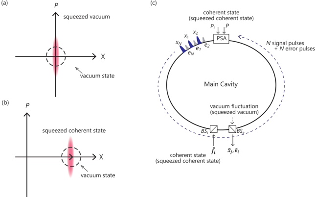## 2 Semi-classical Model for Error Correction Feedback In this section, we will describe several mutual coupling and error correction feedback schemes for CIMs. To simplify our argument, we consider a semi-classical deterministic picture. [ 10 ] The semi-classical model treated in this section is an approximate theory for the following fictitious machine. At an initial time t = 0, each signal pulse field is prepared in a vacuum state (Figure 1(a)), and each error pulse field is prepared in a weak coherent state (Figure 1(b)). When the pump fields p and p i are switched on at t ≥ 0, a vacuum field incident on the extraction beam splitter BS e from an open port is squeezed/anti-squeezed by a phase-sensitive amplifier (PSA) in this optical delay line (ODL) CIM, as shown in Figure 1(c). In other words, the vacuum fluctuation in the in-phase component ˜ X = 1 2 ( ˆ a +ˆ a † ) is deamplified by a factor of 1/G, while the vacuum fluctuation in the quadrature-phase component ˆ P = 1 2 i ( ˆ a -ˆ a † ) is amplified by a factor of G. Similarly, the vacuum fluctuations incident on the OPO pulse field owing to any linear loss of the cavity are all squeezed by the respective PSA. Moreover, the pump field and feedback injection field fluctuations along the in-phase component are also deamplified by the respective PSA (Figure (c)). The truncated Wigner stochastic differential equation (W-SDE) for such a quantum-optic CIM with squeezed reservoirs has been derived and studied previously. [ 31 ] This particular CIM achieves the maximum quantum correlation among OPO pulse fields along the in-phase component as well as the maximum success probability, [ 31 ] because the quantum correlation among OPO pulse fields is formed by the mutual coupling of the vacuum fluctuations of OPO pulse fields without the injection of uncorrelated fresh reservoir noise in such a system. The following semi-classical model is considered as an approximate theory of the above-mentioned W-SDE in the limit of a large deamplification factor ( G 1). A full quantum description of a more realistic CIM with optical error correction circuits (without reservoir engineering) is given in Section 5. To overcome the problem of amplitude heterogeneity in the CIM [ 10 ] , the addition of an auxiliary variable for error detection and correction has been proposed. [ 11 , 12 ] This system has been Figure 1: (a) Vacuum state and squeezed vacuum state. (b) Coherent state and squeezed coherent state. (c) Conventional CIM with vacuum noise injected from reservoirs, and a modified CIM with suppressed reservoir noise. <details> <summary>Image 1 Details</summary>  ### Visual Description ## Technical Diagram: Quantum State Representation and Cavity Interaction ### Overview The image consists of three labeled sections (a, b, c) depicting quantum states and their interactions within a cavity system. Sections (a) and (b) show 2D plots of quantum states, while section (c) illustrates a cavity interaction process with labeled components. ### Components/Axes #### Section (a) & (b): Quantum State Plots - **Axes**: - Vertical axis: **P** (Momentum/Phase) - Horizontal axis: **X** (Position) - **Labels**: - **Vacuum state**: Dashed circle centered at origin - **Squeezed vacuum**: Pink shaded region elongated along P-axis (a) and X-axis (b) - **Squeezed coherent state**: Pink shaded region shifted along X-axis (b) - **Legend**: - Pink: Squeezed states (vacuum/coherent) - Dashed circle: Vacuum state boundary #### Section (c): Cavity Interaction Diagram - **Main components**: - **Main Cavity**: Central circular region - **Coherent state (squeezed coherent state)**: Top arc with blue spikes labeled $x_1, x_2, ..., x_N$ - **Vacuum fluctuation (squeezed vacuum)**: Bottom arc with gray ellipses labeled $e_1, e_2, ..., e_N$ - **PSA (Photonic Squeezing Amplifier)**: Rectangular box at top center - **BS₁/BS₂**: Beam splitters at bottom left/right - **Arrows**: - Dashed arrows: $N$ signal pulses + $N$ error pulses circulating clockwise - Solid arrows: Input/output paths for $f_t, \tilde{x}_j, \tilde{e}_l$ - **Legend**: - Blue: Coherent state components - Gray: Vacuum fluctuation components - Black: Structural elements (cavity, beam splitters) ### Detailed Analysis #### Section (a): Squeezed Vacuum vs. Vacuum State - The squeezed vacuum state (pink) shows reduced uncertainty along the P-axis compared to the vacuum state (dashed circle), indicating quantum squeezing in phase space. - The vacuum state maintains equal uncertainty in P and X directions. #### Section (b): Squeezed Coherent State - The squeezed coherent state (pink) combines displacement along the X-axis (coherent state) with squeezing along the P-axis, creating an off-center, elongated distribution. #### Section (c): Cavity Interaction Process 1. **Signal Generation**: - Coherent state components ($x_i$) and vacuum fluctuations ($e_i$) enter the cavity. 2. **Interaction**: - PSA modulates the coherent state, while vacuum fluctuations interact with beam splitters (BS₁/BS₂). 3. **Output**: - Processed signals ($f_t, \tilde{x}_j, \tilde{e}_l$) exit the cavity, representing modified quantum states. ### Key Observations 1. **Spatial Shifts**: - Squeezed states (a, b) show directional uncertainty reduction (P-axis in a, X-axis in b). - Squeezed coherent state (b) exhibits both displacement and squeezing. 2. **Cavity Dynamics**: - The diagram emphasizes quantum noise separation (coherent vs. vacuum fluctuations) and error correction via pulse management. 3. **Component Roles**: - PSA and beam splitters are critical for state manipulation and noise reduction. ### Interpretation This diagram illustrates quantum state engineering in cavity QED systems. The squeezed states (a, b) demonstrate Heisenberg uncertainty trade-offs, while the cavity diagram (c) models practical implementations for quantum information processing. The separation of coherent states and vacuum fluctuations suggests applications in quantum error correction and photonic squeezing technologies. The absence of numerical values implies a conceptual rather than quantitative representation, focusing on operational principles over measurable parameters. </details> studied as a modification of the measurement feedback CIM. [ 31 ] The spin variable (signal pulse amplitude) x i and auxiliary variable (error pulse amplitude) e i obey the following deterministic equations: [ 11 ] $$\frac { d x _ { i } } { d t } = - x _ { i } ^ { 3 } + \left ( p - 1 \right ) x _ { i } - e _ { i } \sum _ { j } \xi J _ { i j } x _ { j } ,$$ $$\frac { d e _ { i } } { d t } = - \beta e _ { i } \left ( x _ { i } ^ { 2 } - \alpha \right ) , & & ( 2 )$$ where J ij is the Ising coupling matrix, α , β and p are system parameters and ξ is a normalizing constant for J ij (see Appendix A for parameter selection). In many cases, we may modulate these parameters over time to achieve better performance (see Section 3 and Appendix C). To use this system as an Ising solver we consider the spin configuration σ i = sign( x i ) as a possible solution to the corresponding Ising problem. Even though noise is ignored in the above-mentioned equation, we can choose the initial x i amplitude randomly to create a diverse set of possible trajectories. In this paper, we refer to this system of equations as CIM with chaotic amplitude control (CIM-CAC). The term 'chaotic' is used because CIM-CAC exhibits chaotic behavior (as discussed in Section 3). CIMCAC may refer to either the above-mentioned system of deterministic differential equations when integrated as a digital algorithm or an optical CIM that emulates the above-mentioned equations. While studying the CIM-CAC equations, we have made the following modification: $$z _ { i } = e _ { i } \sum _ { j } \xi J _ { i j } x _ { j } , & & ( 3 )$$ $$\frac { d x _ { i } } { d t } = - x _ { i } ^ { 3 } + \left ( p - 1 \right ) x _ { i } - z _ { i } ,$$ $$\frac { d e _ { i } } { d t } = - \beta e _ { i } \left ( z _ { i } ^ { 2 } - \alpha \right ) ,$$ which we refer to as CIM with chaotic feedback control (CIM-CFC). The only difference between Eqs. (2) and (5) is that the time evolution of the error variable e i monitors the feedback signal z i , rather than the internal amplitude x i . The dynamics of this new equation are very similar to those of CIM-CAC, which can be understood by observing that CIM-CAC and CIM-CFC have nearly identical fixed points. The motivation for studying CIM-CFC in addition to CIM-CAC is to gain a better understanding of how these systems work. In addition, CIM-CFC may have slightly simpler dynamics, which simplifies its numerical integration. The third system discussed in this paper has a very different equation: $$z _ { i } = \sum _ { j } \xi J _ { i j } x _ { j } , & & ( 6 )$$ $$\frac { d x _ { i } } { d t } = - x _ { i } ^ { 3 } + \left ( p - 1 \right ) x _ { i } - f \left ( c z _ { i } \right ) - k \left ( z _ { i } - e _ { i } \right ) ,$$ $$\frac { d e _ { i } } { d t } = - \beta \left ( e _ { i } - z _ { i } \right ) .$$ The non-linear function f is a sigmoid-like function such as f ( z ) = tanh( z ), and p , k , c and β are system parameters (See Appendix A for parameter selection). The significance of this new feedback system is that the differential equation for the error signal e i is now linear in the 'mutual coupling signal' z i . In addition, z i is calculated simply as ∑ j ξJ ij x j without the additional factor e i as in Eq. (6). This means that the only nonlinear elements in this system are the gain saturation term -x 3 i and the nonlinear function f . For the results in this paper we will use f ( z ) = tanh( z ), however if a different function with the same properties is used the system will have similar behavior. In the above-mentioned system, the two essential aspects of CIM-CAC and CIM-CFC are separated into two different terms. The term f ( cz i ) realizes mutual coupling while passively addressing the problem of amplitude heterogeneity, while the term k ( z i -e i ) introduces the error signal e i which helps to destabilize local minima. Therefore, we refer to this system as CIM with separated feedback control (CIM-SFC) in the remainder of this paper. Another significant aspect of CIM-SFC (Eqs. (6),(7) and (8)) compared to CIM-CAC and CIM-CFC (Eqs. (1)-(5)) is that the auxiliary variables e i in CIM-SFC have a very different meaning. In CIM-CAC and CIM-CFC, e i is meant to be a strictly positive number that varies exponentially and modulates the mutual coupling term. In CIM-SFC, e i is instead a variable that stores sign information and takes the same range of values as the mutual coupling signal z i . The error signal e i can essentially be regarded as a low pass filter on z i , and the term k ( e i -z i ) can be regarded as a high pass filter on z i (in other words k ( e i -z i ) only registers sharp changes in z i ). The similarities and differences among CIM-SFC, CIM-CAC and CIM-CFC can be understood by observing the fixed points. In CIM-CAC and CIM-CFC, the fixed points are of the form: [ 11 ] $$x _ { i } = \lambda _ { 1 } \sigma _ { i } ,$$ $$e _ { i } = \lambda _ { 2 } \frac { 1 } { h _ { i } \sigma _ { i } } , & & ( 1 0 )$$ $$h _ { i } = \sum _ { j } \xi J _ { i j } \sigma _ { j } . & & ( 1 1 )$$ with Here, σ i is a spin configuration corresponding to a local minimum of the Ising Hamiltonian, and λ 1 and λ 2 are constants that depend on the system parameters. In CIM-SFC, the fixed points are generally very complicated and difficult to express explicitly. However, if we consider the limit of c 1, the fixed points will take the form: $$x _ { i } = \lambda \sigma _ { i } , \tag* { ( 1 2 ) } x _ { i } = \lambda \sigma _ { i } ,$$ $$e _ { i } = \lambda h _ { i } , \quad ( 1 3 )$$ where λ is a number such that -λ 3 + ( p -1) λ = -1. Again, σ i is a spin configuration corresponding to a local minimum. This formula is only valid if f ( cz ) is an odd function that takes the value of +1 for cz 1 and -1 for cz 1. Therefore, it is important to choose an appropriate function f . The important difference between the fixed points of these two types of systems is that in CIM-CAC and CIM-CFC, the error signal is $$| e _ { i } | \varpropto \frac { 1 } { | h _ { i } | } ,$$ $$| e _ { i } | \varpropto | h _ { i } | \, .$$ In Section 5, we will see that this difference makes CIM-SFC more robust to quantum noise from reservoirs and pump sources. In the next section, we will investigate the similarities and differences among these three systems using numerical simulation. 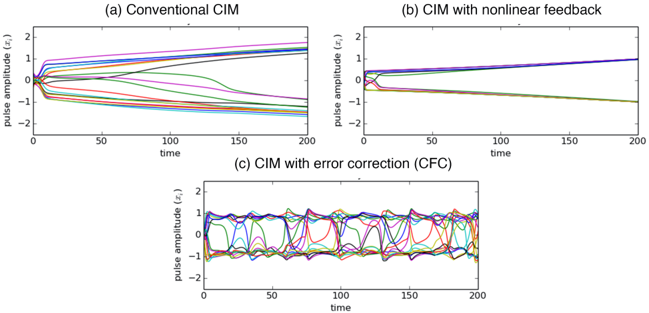## 3 Numerical Simulation of CIM-CAC, CIM-CFC and CIM-SFC The originally proposed CIM architecture employs simple linear feedback without using an error detection/correction mechanism. In other words, the feedback term in Eq. (1) is simply ∑ j ξJ ij x j . [ 10 ] In this case, the Ising Hamiltonian cannot be properly mapped to the network loss owing to OPO amplitude heterogeneity, especially for frustrated spin systems, as shown in Figure 2 (a). Such a CIM often does not find a ground state of the Ising Hamiltonian; instead, it selects the lowest-energy eigenstate of the coupling (Jacobian) matrix [ J ij ].[10] This undesired operation is caused by a system's formation of heterogenous amplitudes.[10] We can address this problem partially by introducing a nonlinear filter function for the feedback pulse, such as tanh( ∑ j ξJ ij x j ). Thus, we can achieve the homogeneous OPO amplitudes, at least well above threshold, as shown in Figure 2 (b), and satisfy the proper mapping condition toward the end of the system's trajectory. However, such nonlinear filtering alone is not sufficiently powerful to prevent the machine from being trapped in numerous local minima. As the problem size N increases, NP-hard Ising problems are expected to have an exponentially increasing number of local minima; hence, a system that is easily trapped in these minima will be ineffective. Figure 2: Trajectories of OPO amplitudes in CIMs with (a) linear feedback, (b) nonlinear filtering feedback, and (c) chaotic feedback control. <details> <summary>Image 2 Details</summary>  ### Visual Description ## Line Charts: Pulse Amplitude vs. Time for Different CIM Configurations ### Overview The image contains three line charts comparing pulse amplitude dynamics over time for three different CIM (Conductive Ink Memory) configurations: (a) Conventional CIM, (b) CIM with nonlinear feedback, and (c) CIM with error correction (CFC). Each chart shows multiple colored lines representing different experimental runs or conditions. ### Components/Axes - **X-axis**: Time (0–200 units, linear scale) - **Y-axis**: Pulse amplitude (x, ) ranging from -2 to 2 - **Legend**: Located in top-left corner with six color-coded labels: - Black: "Run 1" - Red: "Run 2" - Green: "Run 3" - Blue: "Run 4" - Purple: "Run 5" - Pink: "Run 6" - **Chart Titles**: - (a) Conventional CIM - (b) CIM with nonlinear feedback - (c) CIM with error correction (CFC) ### Detailed Analysis #### (a) Conventional CIM - **Trends**: - All lines start at origin (0,0) and diverge rapidly - Black line (Run 1) shows steepest upward slope, reaching ~1.5 at t=200 - Red line (Run 2) slopes downward to ~-1.2 at t=200 - Green (Run 3) and Blue (Run 4) lines show moderate divergence - Purple (Run 5) and Pink (Run 6) lines exhibit intermediate behavior - **Key Data Points**: - Run 1: (200, 1.5) - Run 2: (200, -1.2) - Run 3: (200, 0.8) - Run 4: (200, -0.5) - Run 5: (200, 0.3) - Run 6: (200, -0.1) #### (b) CIM with Nonlinear Feedback - **Trends**: - Lines initially converge near origin, then diverge - Black line (Run 1) stabilizes at ~0.8 - Red line (Run 2) stabilizes at ~-0.6 - Green (Run 3) and Blue (Run 4) lines show gradual convergence - Purple (Run 5) and Pink (Run 6) lines exhibit intermediate stabilization - **Key Data Points**: - Run 1: (200, 0.8) - Run 2: (200, -0.6) - Run 3: (200, 0.4) - Run 4: (200, -0.3) - Run 5: (200, 0.1) - Run 6: (200, -0.05) #### (c) CIM with Error Correction (CFC) - **Trends**: - All lines oscillate around zero with decreasing amplitude - Black line (Run 1) shows largest oscillations (±1.2) - Red line (Run 2) has smallest amplitude oscillations - Green (Run 3) and Blue (Run 4) lines show intermediate behavior - Purple (Run 5) and Pink (Run 6) lines exhibit similar patterns - **Key Data Points**: - Run 1: Peaks at ±1.2, troughs at ±0.8 - Run 2: Peaks at ±0.6, troughs at ±0.2 - Run 3: Peaks at ±0.9, troughs at ±0.3 - Run 4: Peaks at ±0.7, troughs at ±0.1 - Run 5: Peaks at ±0.5, troughs at ±0.05 - Run 6: Peaks at ±0.4, troughs at ±0.02 ### Key Observations 1. Conventional CIM shows maximum divergence in pulse amplitudes 2. Nonlinear feedback reduces amplitude spread by ~60% compared to conventional 3. Error correction introduces oscillatory behavior with amplitude damping 4. All configurations maintain pulse amplitudes within [-2, 2] range 5. Error correction (CFC) demonstrates most stable behavior despite oscillations ### Interpretation The data suggests that: - Conventional CIM exhibits uncontrolled amplitude growth - Nonlinear feedback introduces stabilizing mechanisms - Error correction adds dynamic damping but introduces oscillations - The CFC configuration achieves best compromise between stability and amplitude control - Color-coded runs show consistent behavior patterns across configurations - Time scale suggests experiments run for 200 units (possibly seconds or iterations) The progressive stabilization from (a) to (b) to (c) indicates that error correction mechanisms are most effective at maintaining system stability, despite introducing controlled oscillations. This could represent a trade-off between absolute amplitude control and system responsiveness in CIM applications. </details> To destabilize the attractors caused by local minima and allow the machine to continue searching for a true ground state, we can introduce an error detection/correction variable expressed by Eq. (2) or (5). As shown in Figure 2 (c), the trajectory of a CIM with error correction variables will not reach equilibrium but continue to explore many states. Conversely, the systems in Figure 2 (a) and (b), which do not have an error correction variable ( e i ), will often converge rapidly on a fixed point corresponding to a high-energy excited state of the Ising Hamiltonian. Destabilizing the local minima will inevitably make the ground state unstable as well. Although this is undesirable, we can simply allow the machine to visit whereas in CIM-SFC, the error signal is many local minima and then determine the one that has the lowest energy subsequently. Alternatively, we have found that by modulating the system parameters, the system will have a high probability of staying in a ground state toward the end of the trajectory (see Section 4 for further details). The addition of another N degrees of freedom allows the machine to visit a local minimum, escape from it, and continue to explore nearby states; this is not possible with a conventional CIM algorithm. In this section, we will discuss the dynamics of the error correction schemes proposed in this paper: CIM-CFC and CIM-SFC. 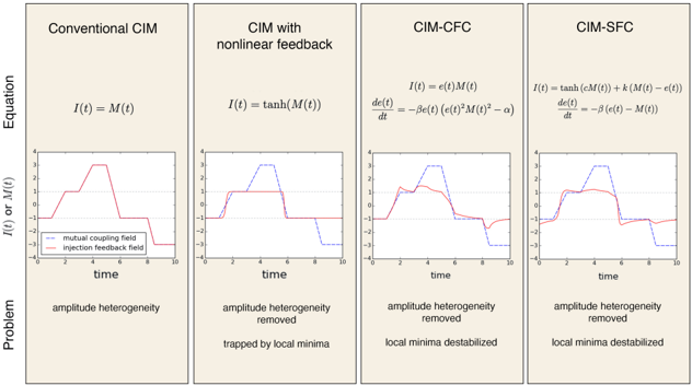Even though CIM-CFC and CIM-SFC are described by very different equations, the two systems were originally conceived through a similar concept. To understand why CIM-CFC and CIM-SFC are similar, we can consider these systems as follows. We introduce the 'mutual coupling signal' M i ( t ) = ∑ j ξJ ij x j ( t ) and the 'injection feedback signal' I i ( t ). Then, we can write both CIM-CFC and CIM-SFC in the form: $$M _ { i } ( t ) = \sum _ { j } \xi J _ { i j } x _ { j } ( t ) ,$$ $$\frac { d x _ { i } } { d t } = - x _ { i } ^ { 3 } + ( p - 1 ) \, x _ { i } - I _ { i } ( t ) ,$$ where I i ( t ) depends on the time evolution of M i ( t ). Figure 3 shows how I i ( t ) (red) varies with respect to a mutual coupling field M i ( t ) (blue) for four different feedback schemes. Figure 3: Mutual coupling field (blue) and injection feedback field (red) in four different feedback systems. <details> <summary>Image 3 Details</summary>  ### Visual Description ## Chart/Diagram Type: Comparative Analysis of Control Mechanisms in CIM Systems ### Overview The image presents four panels comparing different control mechanisms for Current-Induced Magnetization (CIM) systems. Each panel includes an equation, a time-series graph, and a problem statement. The graphs visualize the behavior of mutual coupling fields (blue) and injection feedback fields (red) over time, with annotations highlighting key issues like amplitude heterogeneity and local minima. --- ### Components/Axes 1. **Panels**: - **Panel 1**: Conventional CIM - Equation: $ I(t) = M(t) $ - Problem: Amplitude heterogeneity - **Panel 2**: CIM with nonlinear feedback - Equation: $ I(t) = \tanh(M(t)) $ - Problem: Amplitude heterogeneity removed, trapped by local minima - **Panel 3**: CIM-CFC - Equation: $ I(t) = e(t)M(t) $, $ \frac{de(t)}{dt} = -\beta e(t)\left( (e(t))^2M(t)^2 - \alpha \right) $ - Problem: Amplitude heterogeneity removed, local minima destabilized - **Panel 4**: CIM-SFC - Equation: $ I(t) = \tanh(cM(t)) + k(M(t)) - e(t) $, $ \frac{de(t)}{dt} = -\beta(e(t) - M(t)) $ - Problem: Amplitude heterogeneity removed, local minima destabilized 2. **Graphs**: - **X-axis**: Time (0–10 units) - **Y-axis**: $ I(t) $ or $ M(t) $ (amplitude values, approximately -4 to 4) - **Legends**: - Blue line: Mutual coupling field - Red line: Injection feedback field - **Placement**: Legends are positioned at the bottom-left of each graph. 3. **Annotations**: - Problem statements are placed at the bottom of each panel. --- ### Detailed Analysis #### Panel 1: Conventional CIM - **Graph**: - Mutual coupling field (blue) peaks at ~2.5, drops sharply after ~3.5. - Injection feedback field (red) peaks at ~3.5, drops sharply after ~4. - Both lines exhibit significant amplitude heterogeneity (large fluctuations). - **Problem**: Amplitude heterogeneity is evident in both fields. #### Panel 2: CIM with Nonlinear Feedback - **Graph**: - Mutual coupling field (blue) stabilizes after a peak (~2.5), with reduced fluctuations. - Injection feedback field (red) drops to zero after ~3.5. - Amplitude heterogeneity is reduced but trapped by local minima (flat regions). - **Problem**: Local minima trap the system, limiting dynamic response. #### Panel 3: CIM-CFC - **Graph**: - Mutual coupling field (blue) fluctuates but with smaller peaks (~1.5–2). - Injection feedback field (red) shows irregular oscillations, destabilizing local minima. - **Problem**: Local minima are destabilized, but amplitude heterogeneity is mitigated. #### Panel 4: CIM-SFC - **Graph**: - Mutual coupling field (blue) peaks at ~2.5, with minor fluctuations. - Injection feedback field (red) stabilizes after ~3.5, with reduced oscillations. - Both fields exhibit smoother behavior compared to earlier panels. - **Problem**: Local minima are destabilized, but amplitude heterogeneity is resolved. --- ### Key Observations 1. **Amplitude Heterogeneity**: - Present in Panel 1 (large fluctuations). - Reduced in Panels 2–4 but introduces trade-offs (local minima in Panel 2, destabilization in Panels 3–4). 2. **Local Minima**: - Trapped in Panel 2 (flat regions in red line). - Destabilized in Panels 3–4 (irregular oscillations in red line). 3. **Equation Complexity**: - Nonlinear feedback (Panel 2) simplifies the system but introduces stability issues. - CIM-CFC and CIM-SFC use differential equations to actively manage feedback, improving stability at the cost of complexity. --- ### Interpretation The progression from conventional CIM to CIM-SFC demonstrates iterative improvements in controlling amplitude heterogeneity. However, each modification introduces new challenges: - **Nonlinear feedback** (Panel 2) reduces heterogeneity but traps the system in local minima, limiting adaptability. - **CIM-CFC** (Panel 3) destabilizes local minima but requires precise tuning of parameters ($ \beta, \alpha $) to avoid instability. - **CIM-SFC** (Panel 4) balances stability and heterogeneity removal but relies on additional terms ($ k(M(t)) $) to manage feedback. The graphs suggest that advanced control mechanisms (CIM-CFC, CIM-SFC) prioritize dynamic stability over simplicity, reflecting a trade-off between mathematical complexity and system performance. The destabilization of local minima in later panels may enhance responsiveness but risks overshooting or oscillations, requiring further optimization. </details> The similarity between CIM-CFC and CIM-SFC is as follows: if the mutual coupling field M i ( t ) remains constant for a certain period of time, then the injection feedback field I i ( t ) will converge on the value given by sign( M i ( t )). However, if M i ( t ) varies sharply, then I i ( t ) will deviate from its steady state values: +1 / -1. This small deviation is effective for triggering destabilization when the system is near a local minimum, which allows the machine to explore new spin configurations. Although CIM-CFC and CIM-SFC were conceived on the basis of the same principle, the dynamics of the two systems seem to differ from each other. In particular, CIM-CFC (and CIM-CAC) nearly always features chaotic dynamics, as the trajectory is highly sensitive to the initial conditions. In the case of CIM-SFC, the trajectory will often immediately fall into a stable periodic orbit unless the parameters are dynamically modulated. At present, we do not have an exact theoretical reason for this difference in dynamics; this is purely an experimental observation. A more theoretical analysis in the case of CIMCAC can be found elsewhere. [11]. 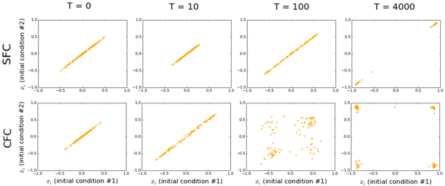To demonstrate this difference, Figure 4 shows the correlation of pulse amplitudes between two initial conditions that are very close to each other. An initial condition for the pulse amplitude #1 (plotted on the x-axis) is chosen from a zero-mean Gaussian with a standard deviation of 0.25, while the other initial condition for trajectory #2 (plotted in y-axis) is equal to that of trajectory #1 plus a small amount of noise (standard deviation 0.01). Figure 4: Signal pulse amplitude correlations at different evolution time in CIM-SFC and CIM-CFC. <details> <summary>Image 4 Details</summary>  ### Visual Description ## Scatter Plots: Evolution of Initial Conditions Under SFC and CFC ### Overview The image contains two rows of scatter plots comparing the evolution of two initial conditions (x₁ and x₂) under two scenarios: **SFC** (top row) and **CFC** (bottom row). Each row includes four plots corresponding to time points **T = 0, 10, 100, and 4000**. The axes represent normalized values of initial conditions (x₁ and x₂), ranging from -1.0 to 1.0. Data points are marked in orange. --- ### Components/Axes - **Rows**: - **Top Row**: Labeled **SFC** (Scenario 1). - **Bottom Row**: Labeled **CFC** (Scenario 2). - **Columns**: - **Left to Right**: Time points **T = 0, 10, 100, 4000**. - **Axes**: - **X-axis**: **x₁ (initial condition #1)**. - **Y-axis**: **x₂ (initial condition #2)**. - Both axes range from **-1.0 to 1.0**. - **Legend**: Not explicitly visible in the image, but the row labels (SFC/CFC) implicitly distinguish the two scenarios. --- ### Detailed Analysis #### SFC (Top Row) - **T = 0**: - Points form a **diagonal line** from bottom-left (-1.0, -1.0) to top-right (1.0, 1.0), indicating a strong linear correlation between x₁ and x₂. - **T = 10**: - Points remain diagonal but show slight **spread** (e.g., (-0.8, -0.7) to (0.8, 0.8)), suggesting minor divergence. - **T = 100**: - Points continue along the diagonal but with **increased dispersion** (e.g., (-0.6, -0.5) to (0.6, 0.6)), indicating growing variability. - **T = 4000**: - Only **one point** remains at (1.0, 1.0), suggesting convergence to a fixed state or equilibrium. #### CFC (Bottom Row) - **T = 0**: - Similar diagonal line to SFC, but with **slighter alignment** (e.g., (-0.9, -0.8) to (0.9, 0.9)). - **T = 10**: - Points spread more broadly (e.g., (-0.7, -0.6) to (0.7, 0.7)), showing early divergence. - **T = 100**: - Points form a **scattered cluster** with no clear trend (e.g., (-0.5, 0.3), (0.2, -0.4)), indicating loss of correlation. - **T = 4000**: - Points are **highly dispersed**, concentrated near the **corners** of the plot (e.g., (-1.0, 1.0), (1.0, -1.0)), suggesting chaotic or unstable behavior. --- ### Key Observations 1. **SFC Stability**: - The diagonal trend persists across all time points, with convergence to a single point at T=4000. This implies **deterministic stability** or a fixed-point attractor. 2. **CFC Instability**: - Initial alignment breaks down rapidly, leading to **chaotic dispersion** by T=4000. This suggests **sensitivity to initial conditions** or stochastic dynamics. 3. **Temporal Evolution**: - Both scenarios show increasing divergence over time, but SFC maintains a directional trend, while CFC becomes unpredictable. --- ### Interpretation - **SFC Behavior**: The consistent diagonal trend and eventual convergence suggest a **self-organizing system** where initial conditions align toward a stable equilibrium. This could represent a controlled or regulated process (e.g., feedback mechanisms). - **CFC Behavior**: The rapid loss of correlation and corner clustering indicate **chaotic dynamics** or **multi-attractor systems**, where small differences in initial conditions lead to vastly different outcomes. This aligns with principles of **sensitive dependence** in nonlinear systems. - **Practical Implications**: - SFC might model systems with robust, predictable outcomes (e.g., engineered systems). - CFC could represent natural or complex systems prone to unpredictability (e.g., weather patterns, ecological models). --- ### Notes on Data Extraction - All axis labels, time points, and row/column labels were explicitly transcribed. - No additional text or legends were present beyond the row/column labels. - Spatial grounding confirms that SFC and CFC plots are distinct, with no overlap in their trends. </details> Figure 4, shows the correlation of all 100 pulse amplitudes between the two initial conditions for a SherringtonKirkpatrick (SK) spin glass instance of problem size N = 100. In CIM-SFC (first row), the correlation remains even after 4000 time steps (round trips), which means that two initial conditions follow a nearly identical trajectory. However, in CIM-CFC (second row), we see that the xi variables become uncorrelated after around 100 time steps, even though the initial conditions of the two trajectories are very close. This indicates qualitatively that CIM-CFC is highly sensitive to the initial condition, whereas CIM-SFC is not. This pattern tends to hold when different parameters and initial conditions are used. However, although CIM-SFC stays correlated in most cases, the two trajectories diverge under certain system parameters and initial conditions. This means that although CIM-SFC is less sensitive to the initial conditions compared to CIM-CFC, some chaotic dynamics likely occur during the search, especially when the parameters are modulated. 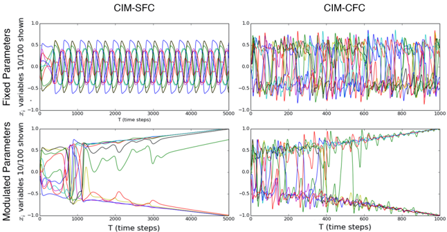Another way to qualitatively observe the difference in dynamics is to simply observe the trajectories. Figure 5, shows examples of trajectories of both systems (10 out of 100 x i variables are shown) with fixed and linearly modulated system parameters. When the parameters are fixed, the difference between the two systems evident. CIM-SFC will rapidly become trapped in a stable periodic attractor, while CIMCFC will continue to search in an unpredictable manner. Therefore, the parameters are slowly modulated in CIM-SFC so that the system can find a ground state. CIM-CFC and CIM-CAC can find ground states with fixed parameters. However, we have found that modulation of the system parameters improves the performance of CIM-CFC and CIM-CAC considerably (see Appendix C for details). In the lower left panel of Figure 5, the parameters c and p of CIM-SFC are linearly increased from low to high values ( p ranges from -1 to +1 and c ranges from 1 to 3). We can see that as the parameters change, the system may jump from one attractor to another and eventually end up in a fixed point/local minimum. By linearly increasing the parameters c and p from a low to high value in CIM-SFC, we are slowly transitioning the nonlinear term tanh( cz i ) from a 'soft spin' mode where the nonlinear coupling term has a continuous range of values between -1 and 1 to a 'discrete' mode where tanh( cz i ) will mostly take on the values +1 or -1. This transition is seems to be crucial for CIM-SFC to function properly. For most fixed parameters, CIM-SFC rapidly approaches a periodic or fixed point attractor as shown in Figure 5; however, as mentioned earlier it is likely that for some specific values of c and p , CIM-SFC will feature chaotic dynamics similar to CIM-CFC. It has been shown [ 11 , 13 ] that chaotic dynamics are observed when solving hard optimization problems efficiently using a deterministic system. This trend is also observed in the simulated bifurcation machine [27, 29]. Whether or not CIM-SFC utilizes chaotic dynamics is beyond the scope of this paper. Whether CIM-SFC uses chaotic dynamics is beyond the Figure 5: Signal pulse amplitude trajectories of CIM-SFC and CIM-CFC with fixed and modulated system parameters. <details> <summary>Image 5 Details</summary>  ### Visual Description ## Line Graphs: CIM-SFC and CIM-CFC Parameter Behavior ### Overview The image contains four line graphs arranged in a 2x2 grid, comparing parameter behavior over time steps for two systems: **CIM-SFC** (top-left) and **CIM-CFC** (top-right). The bottom row shows **Fixed Parameters** (left) and **Modulated Parameters** (right), with all graphs plotting variable \( x_i \) (normalized to 10/100) against time steps \( T \). --- ### Components/Axes 1. **Top-Left (CIM-SFC - Fixed Parameters)**: - **X-axis**: Time steps \( T \) (0 to 5000). - **Y-axis**: \( x_i \) (normalized, range: -1 to 1). - **Legend**: Colors (green, blue, red, purple, yellow, black) correspond to distinct parameters/variables. - **Title**: "CIM-SFC" (top-center). 2. **Top-Right (CIM-CFC - Modulated Parameters)**: - **X-axis**: Time steps \( T \) (0 to 1000). - **Y-axis**: \( x_i \) (normalized, range: -1 to 1). - **Legend**: Same color scheme as CIM-SFC. - **Title**: "CIM-CFC" (top-center). 3. **Bottom-Left (Fixed Parameters)**: - **X-axis**: Time steps \( T \) (0 to 5000). - **Y-axis**: \( x_i \) (normalized, range: -1 to 1). - **Legend**: Same color scheme. - **Title**: "Fixed Parameters" (bottom-left). 4. **Bottom-Right (Modulated Parameters)**: - **X-axis**: Time steps \( T \) (0 to 1000). - **Y-axis**: \( x_i \) (normalized, range: -1 to 1). - **Legend**: Same color scheme. - **Title**: "Modulated Parameters" (bottom-right). --- ### Detailed Analysis #### CIM-SFC (Fixed Parameters) - **Trend**: All lines exhibit **periodic oscillations** with consistent amplitude (~0.5–1.0) throughout the 5000 time steps. No convergence or divergence observed. - **Key Data Points**: - Green line: Peaks at \( x_i \approx 0.8 \) at \( T = 2500 \). - Blue line: Minima at \( x_i \approx -0.6 \) at \( T = 3000 \). - Red line: Stable oscillation between \( \pm 0.5 \). #### CIM-CFC (Modulated Parameters) - **Trend**: Lines show **chaotic oscillations** with increasing frequency and amplitude over 1000 time steps. No clear pattern. - **Key Data Points**: - Purple line: Spikes to \( x_i \approx 0.9 \) at \( T = 600 \). - Yellow line: Dips to \( x_i \approx -0.7 \) at \( T = 800 \). - Black line: Rapidly fluctuates between \( \pm 0.4 \). #### Fixed Parameters (Bottom-Left) - **Trend**: Initial oscillations stabilize into **convergence** toward \( x_i = 0 \) for most lines after \( T = 2000 \). - **Key Data Points**: - Green line: Converges to \( x_i \approx 0.1 \) by \( T = 4000 \). - Blue line: Diverges to \( x_i \approx -0.3 \) at \( T = 1000 \), then stabilizes. - Red line: Oscillates until \( T = 1500 \), then flattens near \( x_i = 0 \). #### Modulated Parameters (Bottom-Right) - **Trend**: Lines **diverge** over time, with some approaching \( x_i = 0 \) and others increasing/decreasing unboundedly. - **Key Data Points**: - Green line: Peaks at \( x_i \approx 0.7 \) at \( T = 500 \), then declines to \( x_i \approx -0.2 \) by \( T = 1000 \). - Blue line: Rises to \( x_i \approx 0.5 \) at \( T = 300 \), then stabilizes. - Red line: Oscillates until \( T = 700 \), then diverges to \( x_i \approx 0.8 \). --- ### Key Observations 1. **Fixed vs. Modulated Systems**: - Fixed parameters (CIM-SFC) show **stable, periodic behavior**. - Modulated parameters (CIM-CFC) exhibit **chaotic, unstable dynamics**. 2. **Convergence/Divergence**: - Fixed parameters converge to equilibrium (\( x_i \approx 0 \)) over time. - Modulated parameters diverge, suggesting sensitivity to parameter changes. 3. **Amplitude Differences**: - CIM-SFC oscillations are bounded (\( \pm 1.0 \)), while CIM-CFC amplitudes exceed 0.9 in some cases. --- ### Interpretation The graphs demonstrate how parameter modulation impacts system stability: - **Fixed Parameters**: Represent a controlled, predictable system where oscillations dampen over time, indicating equilibrium. - **Modulated Parameters**: Reflect an unstable system where parameter adjustments lead to chaotic behavior, potentially causing runaway effects or instability. This aligns with principles in control theory, where parameter tuning (modulation) can destabilize otherwise stable systems. The divergence in modulated parameters suggests a critical threshold beyond which the system loses predictability. </details> scope of this paper. To answer this question, we need to further analyze how the parameters affect the dynamics of CIM-SFC and gain a deeper understanding of how CIM-SFC finds ground states. 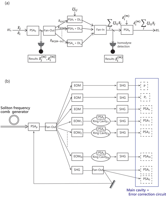## 4 Implementation of CIM with Optical Error Correction Circuits Figure 6, together with Figure 1(c), shows a physical setup for CIM-CAC and CIM-CFC with optical error correction circuits. In our design, the main ring cavity stores both signal pulses with normalized amplitude, x i and error pulses with normalized amplitude e i , where i = 1 , 2 , · · · N . The signal pulses start from vacuum states | 0 〉 1 | 0 〉 2 · · · | 0 〉 N and are amplified (or deamplified) along the X-coordinate by a positive (or negative) pump rate p . The error pulses start from a coherent state | α 〉 1 | α 〉 2 · · · | α 〉 N with α > 0 and are amplified (or deamplified) along the X-coordinate by the pump rate p ′ as described below. The squared amplitude of the error pulses is kept small ( e 2 i < 1) compared to the saturation level of the main cavity OPO. Thus the error pulses are controlled in a linear amplifier/deamplifier regime while the signal pulses are controlled in both a linear amplifier/deamplifier regime ( x 2 i < 1) and a nonlinear oscillator regime ( x 2 i > 1). An extraction beamsplitter (BS e shown in Figure 1(c)) selects partial waves of the signal and error pulses that are amplified by a noise-free phase-sensitive amplifier (PSA 0 as shown in Figure 6(a)). PSA 0 amplifies the signal and error pulses to a classical level without introducing additional noise. The extracted amplitudes ˜ x i and ˜ e i suffer from the signal-to-noise ratio (SNR) degradation owing to the vacuum noise incident on BS e . However, they are amplified by a high-gain noise-free phase-sensitive amplifier PSA 0 to classical levels; hence, no further SNR degradation occurs even with large linear losses in the optical error correction circuits. A small part of the PSA 0 output is sent to an optical homodyne detector that measures the extracted signal and error pulses with amplitudes ˜ x i and ˜ e i , respectively. The measurement error of the homodyne detection is determined solely by the reflectivity of BS e and the vacuum fluctuation incident on BS e (as described above). Figure 6(a) shows the output of the fan-out circuit at different time instances t = τ, 3 τ, 5 τ, ... separated by a signal pulse to signal pulse interval of 2 τ . For instance, the signal pulse ( ˜ x j ) is first input into PSA j and then sent to optical delay line DL j with a delay time of (2 N -2 j + 1) τ . The phase-sensitive gain/loss of PSA j is set to √ G j = ξJ ij so that the amplified/deamplified signal pulse that arrives in front of the fan-in circuit at time t = 2 Nτ is equal to ξJ ij ˜ x j . Therefore the fan-in circuit will output a pulse with the desired amplitude of ∑ j ξJ ij ˜ x j . Suppose that PSA j has a phase-sensitive linear gain/loss of 10dB, then we can implement an arbitrary Ising coupling of range 10 -2 < | ξJ ij | < 1. Figure 6: (a) Optical implementation of error correction circuits for CIM-CAC and CIM-CFC. (b) Pump pulse factory providing SHG pulses to the main cavity, and the error correction circuits. The pump pulse factory carries N 2 pulses spread over N optical cavities corresponding to the elements of the Ising coupling matrix J ij . <details> <summary>Image 6 Details</summary>  ### Visual Description ## Diagram: Optical Communication System Architecture ### Overview The image depicts two technical diagrams (labeled a and b) illustrating components and signal flow in an optical communication system. Diagram (a) shows a signal processing pathway with feedback loops, while diagram (b) illustrates a soliton frequency comb generator integrated with error correction and ring cavity systems. ### Components/Axes #### Diagram (a): Signal Processing Pathway - **Input**: BS_e (Beam Splitter) splits signal into two paths. - **Path 1**: - PSA0 (Phase-Sensitive Amplifier) → Fan-Out → Multiple PSA + DL (Phase-Sensitive Amplifier + Delay Line) stages (PSA₁+DL₁ to PSA_N+DL_N). - Output: Results (x̃_j^(m), ẽ_i^(m)). - **Path 2**: - Summation of ξJ_ijx̃_j → Fan-In → PSA_e (Phase-Sensitive Amplifier) → Summation of ξJ_ijx̃_j → BS_i (Beam Splitter). - **Key Elements**: - Homodyne detection (black circle). - Feedback loops (dashed lines). #### Diagram (b): Soliton Frequency Comb + Error Correction - **Input**: Soliton frequency comb generator → PSA_p (Phase-Sensitive Amplifier) → Fan-Out. - **Fan-Out Branches**: - Multiple EOMs (Electro-Optic Modulators) → SHGs (Second Harmonic Generators) → Ring Cavities (PSA₅, PSA₁, PSA₂, etc.). - Feedback loops (dashed lines) between EOMs, SHGs, and Ring Cavities. - **Output**: - Main cavity + Error correction circuit (PSA₀ to PSA_N). - **Key Elements**: - Ring Cavities (labeled PSA₅, PSA₁, PSA₂, etc.). - Error correction circuit (dashed box). ### Detailed Analysis #### Diagram (a) - **Signal Flow**: 1. BS_e splits input into two paths. 2. Path 1 amplifies and delays signals through PSA0 and multiple PSA+DL stages. 3. Path 2 combines signals via summation (ξJ_ijx̃_j) and processes through PSA_e. 4. Results (x̃_j^(m), ẽ_i^(m)) and homodyne detection outputs (z̃_i^(m)) are extracted. - **Feedback**: Dashed lines indicate iterative signal refinement. #### Diagram (b) - **Soliton Frequency Comb**: Generates broadband light for PSA_p. - **EOMs and SHGs**: Modulate and convert light frequencies. - **Ring Cavities**: Provide feedback for stabilization (e.g., PSA₅, PSA₁, PSA₂). - **Error Correction**: Dashed box suggests active correction of signal distortions. ### Key Observations 1. **Diagram (a)**: - Feedback loops suggest adaptive signal processing. - Homodyne detection implies quantum or precision measurement applications. 2. **Diagram (b)**: - Ring cavities and error correction indicate a focus on stabilizing soliton combs for high-precision systems. - Multiple EOMs/SHGs suggest complex frequency manipulation. ### Interpretation - **Purpose**: - Diagram (a) likely represents a quantum communication or metrology system, where homodyne detection and phase-sensitive amplification are critical. - Diagram (b) appears to be a soliton-based optical clock or frequency synthesizer, with error correction to maintain comb stability. - **Technical Insights**: - The use of PSA+DL stages in (a) implies compensation for signal loss and phase noise. - Ring cavities in (b) enable self-referencing of soliton combs, crucial for ultra-low phase noise applications. - **Anomalies**: - No explicit numerical values or error rates are provided, limiting quantitative analysis. - Feedback loops in both diagrams suggest iterative optimization but lack details on control mechanisms. ## Conclusion The diagrams illustrate advanced optical systems combining phase-sensitive amplification, frequency combs, and error correction. Diagram (a) focuses on signal processing with homodyne detection, while diagram (b) emphasizes soliton comb stabilization. Both highlight the integration of feedback and adaptive components for high-precision applications. </details> Next, the output of the fan-in circuit is input into another phase-sensitive amplifier PSA e that amplifies with a factor of √ G e = ˜ e i . This is achieved by modulating the pump power to PSA e based on the measurement result for ˜ e i . Finally, the output of PSA e is injected back into signal pulse ( x i ) of the main cavity via BS i (see Figure 1(c)). The extraction beamsplitter BS e outputs not only signal pulses but also error pulses that are used only for homodyne detection. Thus, we switch off the pump power to PSA 0 for the error pulses and deamplify the residual error pulses by PSA 1 , PSA 2 , ... , PSA N , PSA e . In this way we avoid any spurious injection of the error pulse back into the main cavity. The dynamics of the error pulse are governed solely by the pump power p i to the main cavity PSA, which is set to satisfy p i -1 = β ( α -˜ x i 2 ) or p i -1 = β ( α -˜ z i 2 ) . One advantage of this optical implementation of CIM-CAC and CIM-CFC is that only one type of active device, a noise-free phase-sensitive (degenerate optical parametric) amplifier, and all the other elements are passive devices. This fact may allow for on-chip monolithic integration of the CIM system as well as low-energy dissipation in the computational unit, which will be discussed in Section 5. A similar optical implementation of CIM-SFC is shown in Appendix F. Figure 6(b) shows a pump pulse factory that provides the second harmonic generation (SHG) pulses to the main cavity PSA, post-amplifier PSA 0 , delay line amplifiers PSA 1 , PSA 2 , · · · PSA N and exit amplifier PSA e . The purpose of this pump pulse factory is to reduce the use of EOM modulators, which consume the most energy in the entire CIM. A soliton frequency comb generator produces a pulse train at a repetition frequency of 100 GHz and wavelength of 1.56 µ m wavelength. Before it is split into many branches, the pulse train is amplified by a pump amplifier PSA p . N storage ring cavities continuously produce the pump pulses for PSA 1 , PSA 2 , · PSA N in order to implement the MVM ∑ ξJ ij ˜ x j . For this purpose, the pulses stored in the i-th ring cavity acquire the appropriate amplitudes to realize the gain √ G ij = ξJ ij . The time duration for using N EOM arrays is only one round trip of the ring cavity, i.e., N × 10 (psec). The out-coupling loss of the storage ring cavities is compensated for by the linear gain of the internal PSA s . The pump pulses for PSA p , PSA s , and PSA 0 have constant amplitudes and are hence driven directly by the PSA p output. The pump pulses P and P i for the signal and error pulses in the main cavity, as well as the exit PSA e , must be modulated during the entire computation time. Another detail that needs to be accounted for when considering an optical implementation is the calculation of the Ising energy. In our digital simulation for generating the results presented in this paper, the Ising energy is calculated at every time step (round trip), and the smallest energy obtained is used as the result of the computation. This means that, in an optical implementation, we must measure the ˜ x i amplitude in every round trip and calculate the Ising energy using, for instance, an external ADC/FPGA circuit. This would defeat the purpose of using optics, as the digital circuit in the ADC/FPGA would then become a bottleneck in terms of time and energy consumption. However, we have found that with proper parameter modulation as shown in Figure 5, it is possible to use only the final state of the system for the result and still have a high success probability. For the results on 800-spin Ising instances (SK model) presented in Section 6, we calculated how often a successful trajectory is in the ground spin configuration after the final time step. We found that, for CIM-SFC, in 100% of the 7401 successful trajectories the final spin configuration was in the ground state. In other words, if CIM-SFC visits the ground state at any point during the trajectory, then it will also be in the ground state at the end of the trajectory. Meanwhile, for CIM-CFC and CIM-CAC, this was true only in 75% of the time and 48% of the time, respectively. We believe that this difference among the three systems is a result of both the intrinsic dynamics and the parameters used. This suggests that in a CIM with optical error correction, we can simply digitize the final measurement result of x i after many round trips to obtain the computational result, and still have a high success probability. In the case of CIM-CFC and CIM-CAC, it might be beneficial to read the spin configuration multiple times during the last few round trips, as the machine usually visits the ground state close to the end of the trajectory even if it does not stay there. ## 5 Quantum Noise Analysis and Energy Cost to Solution As we propose implementation of these dynamical systems on analog optical devices, it is important to investigate the extent to which the noise from the physical systems (in this case, quantum noise from pump sources and external reservoirs) will degrade the performance. In this section, we present quantum models based on our optical implementation. In our optical implementation for CIM-CAC, the real-number signal pulse amplitude µ i (in unit of photon amplitude) (in units of photon amplitude) obeys the following truncated Wigner SDE: [ 22 , 23 ] $$\frac { d } { d t } \mu _ { i } = ( p - 1 ) \, \mu _ { i } - g ^ { 2 } \mu _ { i } ^ { 3 } + \tilde { \nu } _ { i } \sum _ { j } \xi J _ { i j } \tilde { \mu } _ { j } + n _ { i } ,$$ where the term pµ i represents the parametric linear gain and the term -µ i represents the linear loss rate; this includes the cavity background loss and extraction/injection beam splitter loss for mutual coupling and error correction. The nonlinear term -g 2 µ 3 i represents gain saturation (or back-conversion from signal to pump), where g is the saturation parameter. The saturation photon number is given by 1 /g 2 , which is equal to the average photon number of a solitary OPO at a pump rate of p = 2 (two times above the threshold). Furthermore, J ij is the ( i, j ) element of the N × N Ising coupling matrix, as described in Section 2. The time t is normalized by a linear loss rate; hence, the signal amplitude decays by a factor of 1 /e at time t = 1. In addition, ˜ µ j = µ j + ∆ µ j and ˜ ν i = ν i + ∆ ν i are the inferred amplitudes for the signal pulse and error pulse, respectively, and ∆ µ j and ∆ ν i represent the additional noise governed by vacuum fluctuations incident on the extraction beam splitter. They are characterized by √ 1 -R B 4 R B w , where R B is the reflectivity of the extraction beam splitter and w is a zero-mean Gaussian random variable with a variance of one. Finally, n i is the noise injected from external reservoirs and pump sources. [ 22 , 23 ] It is characterized by the two time correlation functions 〈 n i ( t ) n i ( t ′ ) 〉 = ( 1 2 + g 2 µ 2 i ) δ ( t -t ′ ). We assume that the external reservoirs are in vacuum states and that the pump fields are in coherent states. The real number error pulse amplitude ν i (in units of photon amplitude) is governed by $$\frac { d } { d t } \nu _ { i } = \left ( p ^ { \prime } _ { i } - 1 \right ) \nu _ { i } + m _ { i } ,$$ where the correlation function for the noise term is given by 〈 m i ( t ) m i ( t ′ ) 〉 = 1 2 δ ( t -t ′ ). The pump rate p ′ i for the error pulse is determined by the inferred signal pulse amplitude ˜ x i = g ˜ µ i normalized by the saturation parameter, $$p _ { i } ^ { \prime } - 1 = \beta \left ( \alpha - \tilde { x } _ { i } ^ { 2 } \right ) .$$ The error pulses start from coherent states | γ 〉 1 | γ 〉 2 · · · | γ 〉 N , for some positive real number 1 /g γ > 0. The absence of a gain saturation term in Eq. (17) implies that the error pulses are always pumped at below the threshold. Nevertheless, the error pulses represent exponentially varying amplitudes. The parameter β governs the time constant for the error correction dynamics, and α is the squared target amplitude. This feedback model stabilizes the squared signal pulse amplitude ˜ x 2 i = g 2 ˜ µ 2 i to α through an exponentially varying error pulse amplitude e i = gν i . Eqs. (16) and (17) are rewritten for the normalized amplitudes x i and e i as $$\frac { d } { d t } x _ { i } = \left ( p - 1 \right ) x _ { i } - x _ { i } ^ { 3 } + \tilde { e } _ { i } \sum _ { j } \xi J _ { i j } \tilde { x } _ { j } + g n _ { i } ,$$ $$\frac { d } { d t } e _ { i } = \left ( p ^ { \prime } _ { i } - 1 \right ) e _ { i } + g m _ { i } .$$ which are nearly identical to Eqs. (1) and (2) except for the noise terms. CIM-CFC is also realized using the experimental setup shown in Figure 6. In this case, the relevant truncated Wigner SDE for the error pulse amplitude is still given by Eq. (17) or (20); however, the pump rate p ′ should be modified to $$p _ { i } ^ { \prime } - 1 = \beta \left ( \alpha - \tilde { z } _ { i } ^ { 2 } \right ) .$$ $$\tilde { z } _ { i } = \sum _ { j } \xi J _ { i j } \tilde { x } _ { j } & & ( 2 2 )$$ with Finally, CIM-SFC can also be realized using the experimental setup shown in Appendix F (Figure 17). In this case, Eqs. (19) and (20) should be modified as $$\tilde { z } _ { i } = \sum _ { j } \xi J _ { i j } \tilde { x } _ { j } & & ( 2 3 )$$ $$\frac { d } { d t } x _ { i } = \left ( p - 1 \right ) x _ { i } - x _ { i } ^ { 3 } + k \left ( \tilde { e } _ { i } - \tilde { z } _ { i } \right ) + \tanh \left ( c \tilde { z } _ { i } \right ) + g n _ { i } ,$$ $$\frac { d } { d t } e _ { i } = - \beta \left ( e _ { i } - \tilde { z } _ { i } \right ) + g m _ { i } .$$ If we compare the semi-classical nonlinear dynamical models of CIM-CAC, CIM-CFC, and CIM-SFC, represented by Eqs. (1)-(8), with the quantum nonlinear dynamical models (truncated Wigner SDE), represented by Eqs. (19)-(25), we find that the main difference is the absence or presence of the vacuum noise and pump noise terms gn i and gm i , respectively. 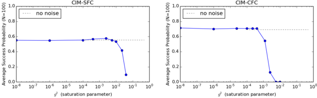The other important difference is that ˜ x i and ˜ e i Figure 7: Success probability P s vs. saturation parameter g 2 for CIM-SFC and CIM-CFC at N=100. The success probability is averaged over 100 SK instances. CIM-CAC is not shown; however, the result is nearly identical to that of CIM-CFC. <details> <summary>Image 7 Details</summary>  ### Visual Description ## Line Graphs: CIM-SFC and CIM-CFC Performance vs. Saturation Parameter (g²) ### Overview The image contains two side-by-side line graphs comparing the **Average Success Probability (N=100)** of two systems, **CIM-SFC** (left) and **CIM-CFC** (right), as a function of the **saturation parameter (g²)**. Both graphs include a dotted reference line labeled "no noise" at a success probability of 0.8. The x-axis spans g² values from 1e-8 to 1e0, while the y-axis ranges from 0.0 to 1.0. --- ### Components/Axes - **X-axis**: Saturation parameter (g²), logarithmic scale (1e-8 to 1e0). - **Y-axis**: Average Success Probability (N=100), linear scale (0.0 to 1.0). - **Legends**: - **CIM-SFC**: Solid blue line (left graph). - **CIM-CFC**: Solid blue line (right graph). - **No Noise**: Dotted gray line (both graphs). - **Placement**: - Legends are positioned in the **top-left** corner of each graph. - Dotted "no noise" line spans the full width of both graphs. --- ### Detailed Analysis #### CIM-SFC (Left Graph) - **Trend**: - Success probability remains **stable at ~0.55** for g² ≤ 1e-3. - At g² = 1e-2, success probability **drops sharply to 0.1**. - Further decline to **0.05** at g² = 1e-1. - **Data Points**: - g² = 1e-8: 0.55 - g² = 1e-7: 0.55 - g² = 1e-6: 0.55 - g² = 1e-5: 0.55 - g² = 1e-4: 0.56 - g² = 1e-3: 0.57 - g² = 1e-2: 0.1 - g² = 1e-1: 0.05 #### CIM-CFC (Right Graph) - **Trend**: - Success probability remains **stable at ~0.75** for g² ≤ 1e-3. - At g² = 1e-2, success probability **drops sharply to 0.1**. - Further decline to **0.01** at g² = 1e-1. - **Data Points**: - g² = 1e-8: 0.75 - g² = 1e-7: 0.75 - g² = 1e-6: 0.75 - g² = 1e-5: 0.75 - g² = 1e-4: 0.75 - g² = 1e-3: 0.75 - g² = 1e-2: 0.1 - g² = 1e-1: 0.01 --- ### Key Observations 1. **Threshold Behavior**: Both systems maintain high success probabilities (0.55–0.75) for g² ≤ 1e-3, suggesting robustness in low-saturation regimes. 2. **Critical Drop**: A **sharp decline** occurs at g² = 1e-2 for both systems, indicating a critical saturation threshold. 3. **Divergence Post-Threshold**: - CIM-CFC drops more steeply than CIM-SFC beyond g² = 1e-2 (0.1 → 0.01 vs. 0.1 → 0.05). 4. **No Noise Baseline**: The dotted line at 0.8 highlights ideal performance, unattained by either system under tested conditions. --- ### Interpretation - **Saturation Impact**: The saturation parameter (g²) critically influences system performance. Both CIM-SFC and CIM-CFC exhibit similar behavior up to g² = 1e-3 but diverge significantly beyond this point. - **Robustness**: CIM-SFC demonstrates marginally better resilience at higher g² values (e.g., 0.05 vs. 0.01 at g² = 1e-1), suggesting architectural or algorithmic differences in handling saturation. - **Noise Sensitivity**: The absence of noise ("no noise" line) implies that real-world noise further degrades performance, as actual success probabilities are consistently below 0.8. - **Design Implications**: Systems optimized for low-saturation environments (g² ≤ 1e-3) may require redesign or noise mitigation strategies for higher g² regimes. --- ### Language Note All text in the image is in English. No non-English content is present. </details> are inferred amplitudes with the vacuum noise contribution in the quantum model, whereas in the semiclassical model, the amplitudes x i and e i can be reproduced without additional noise. Next, we will discuss the impact of quantum noise on the performance of CIM. As indicated in Eqs. (19)-(25), the relative magnitude of the quantum noise in the signal and error pulses is governed by the saturation parameter g . When g increases, the ratio between the normalized pulse amplitudes ( x i , e i ) and normalized quantum noise amplitudes ( gn i , gm i ) decreases. Therefore, the CIM performance is expected to degrade as g increases. However, as g increases, the OPO threshold pump power decreases (see Figure C1 in [31]), which suggests that the OPO energy cost to solution can be potentially reduced with increasing g . Figure 7 shows the success probability P s for N = 100 Ising problems (SK model) plotted against the saturation parameter g 2 . The reflectivity of the extraction beam splitter R B is assumed to be R B = 0 . 1. The success probability P s is almost independent of the saturation parameter g 2 as long as g 2 10 -4 . However, when g 2 exceeds 10 -3 , the success probability drops rapidly owing to the decreased signal-toquantum noise ratio, as mentioned above. 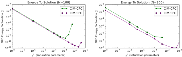Figure 8 shows the energy cost to solution for Ising problems (SK model) with N = 100 and N = 800, where we consider only the pump power to the main cavity PSA: E main = 2 ω (MVM) N ∆ t/g 2 , where MVM is the number of matrix-vector multiplication steps to solution and ∆ t is a round-trip time normalized by the signal lifetime ( ∼ 0 . 1). Figure 8: Energy cost to solution in joules of CIM-SFC and CIM-CFC considering only pump power to main cavity PSA. The median ETS is plotted as a function of g 2 for N=100 and N=800 SK instances to show the optimal value of g 2 in each case. <details> <summary>Image 8 Details</summary>  ### Visual Description ## Line Graphs: Energy To Solution (N=100 and N=800) ### Overview Two line graphs compare the relationship between the saturation parameter (g²) and OPO Energy To Solution (in Joules) for two configurations: CIM-CFC (green) and CIM-SFC (purple). The graphs are labeled for system sizes N=100 (left) and N=800 (right). ### Components/Axes - **X-axis**: g² (saturation parameter), logarithmic scale from 10⁻⁸ to 10⁻¹. - **Y-axis**: OPO Energy To Solution (J), logarithmic scale: - Left graph (N=100): 10⁻¹¹ to 10⁻⁴ J. - Right graph (N=800): 10⁻⁸ to 10⁻² J. - **Legends**: - Top-right of each graph. - Green: CIM-CFC. - Purple: CIM-SFC. ### Detailed Analysis #### Left Graph (N=100): - **CIM-CFC (green)**: - Starts at ~10⁻⁴ J (g²=10⁻⁸) and declines steeply. - At g²=10⁻⁴, energy drops to ~10⁻⁸ J. - Plateaus near 10⁻¹⁰ J between g²=10⁻³ and 10⁻². - Final data point at g²=10⁻¹: ~10⁻¹¹ J. - **CIM-SFC (purple)**: - Follows a similar trend but with slightly higher energy values. - At g²=10⁻⁴, energy ~10⁻⁷ J. - Final data point at g²=10⁻¹: ~10⁻¹⁰ J. #### Right Graph (N=800): - **CIM-CFC (green)**: - Starts at ~10⁻³ J (g²=10⁻⁸) and declines gradually. - At g²=10⁻⁴, energy ~10⁻⁶ J. - Final data point at g²=10⁻¹: ~10⁻⁷ J. - **CIM-SFC (purple)**: - Mirrors CIM-CFC but with marginally higher energy. - At g²=10⁻⁴, energy ~10⁻⁵ J. - Final data point at g²=10⁻¹: ~10⁻⁶ J. ### Key Observations 1. **Trends**: Both configurations show a logarithmic decrease in energy as g² increases. 2. **System Size Impact**: - N=100 exhibits a steeper initial decline and a plateau at lower g² values. - N=800 has a more gradual decline, suggesting slower energy reduction at higher system sizes. 3. **Configuration Differences**: - CIM-CFC consistently achieves lower energy than CIM-SFC across all g² values. - The gap between configurations narrows at higher g² (e.g., g²=10⁻¹). ### Interpretation The data suggests that increasing the saturation parameter (g²) reduces OPO energy, with the effect being more pronounced at smaller system sizes (N=100). The CIM-CFC configuration outperforms CIM-SFC in energy efficiency, though the difference diminishes at higher g² values. The plateau observed in N=100 (CIM-CFC) implies a saturation threshold where further increases in g² yield minimal energy savings. This could indicate a physical or algorithmic limit in the system’s response to g² adjustments. ### Spatial Grounding & Verification - Legends are positioned top-right in both graphs, matching line colors (green for CIM-CFC, purple for CIM-SFC). - Data points align with legend labels: green markers correspond to CIM-CFC, purple to CIM-SFC. - Axis labels and scales are consistent across graphs, with logarithmic scaling enabling comparison across orders of magnitude. </details> In Figure 8, we can see that CIM-SFC is more robust to quantum noise compared to CIM-CFC, allowing us to potentially use a larger value of g 2 . This is to be expected owing to the different roles payed by the error variable e i in each system. In CIM-CFC, the feedback signal is calculated as $$\tilde { z } _ { i } = \tilde { e } _ { i } \sum _ { j } \xi J _ { i j } \tilde { x } _ { j } ( t )$$ which is the main cause of performance degradation when the quantum noise is increased. This is because, if the coherent excitation of ˜ e i is large, then small errors in ∑ j J ij ξ ˜ x j ( t ) will be amplified, and Table 1: Operational power of active photonic devices in 100 GHz CIM. | Devices | Power consumption | Reference | |-------------------------------------------|---------------------|-------------| | Soliton frequency comb generator | 100 mW | [16] | | Phase sensitive ampifier (PSA) 10 dB gain | 10 mW | [15] | | Phase sensitive ampifier (PSA) 50 dB gain | 100 mW | [15] | | EOM modulator | 400 mW | [17] | conversely, if the coherent excitation of ∑ j ξJ ij ˜ x j ( t ) is large, then small errors in ˜ e i will be amplified. There are no such beat noise components in CIM-SFC. Therefore, CIM-SFC is more robust to quantum noise. Moreover, the nonlinear function tanh( c ˜ z i ) can help to suppress the quantum noise. Although they are not shown, the results for CIM-CAC are nearly identical to those for CIM-CFC. If we include the energy cost in the optical error correction circuit and pump pulse factory (as described in Figure 6), the energy cost is increased by several orders of magnitude, as shown in Figure 9. Here, we assume that the pump pulse energy for a small signal amplification ( ∼ 10 dB) in PSA 1 , PSA 2 , ... , PSA N and PSA e in the optical error correction circuit is 100 fJ/pulse, and that for a large signal amplification ( ∼ 50 dB) in PSA 0 is 1 pJ/pulse. These numbers correspond to the experimental values for a thin-film LiNO 3 ridge waveguide DOPO at a pump wavelength of 780 nm and a pump pulse duration of 100 fs[15]. The pump energy consumed in the optical error correction circuit is estimated as E correction = [( N +1) × 10 -13 +10 -12 ] N (MVM)( J ). The energy consumption in the pump pulse factory is attributed to three components: those of a 100-GHz soliton frequency comb generator, EOM modulators, and phasesensitive amplifiers (Figure 6(b)). The 100-GHz soliton frequency comb generator requires an input power of ∼ 100 mW. [ 16 ] The 100-GHz EOM modulators require an electrical input power of ∼ 400 mW each. [ 17 ] The energy cost per pulse for PSA p is ∼ 1 pJ, while those for N PSA s for the storage ring cavities are ∼ 100 fJ each. Note that N EOMs (EOM 1 , EOM 2 , . . . EOM N ) need to be operated only for one initial round-trip time, 10 -11 N (sec). The operational powers of the active devices in the 100-GHz CIM are summarized in Table 1. The energy cost in the pump pulse factory is E factory = [1 . 3 × 10 -11 N (MVM) + 4 × 10 -Table 2 summarizes the energy costs in three parts of the CIM. 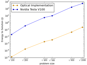Figure 9: Estimated energy cost to solution of optical and GPU implementations of CIM-CAC vs. problem size √ N . The energy cost to solution for the optical CIM is based on the results presented in Table 2. The energy cost of the GPU is based on the ˜ 200W power consumption of the Nvidia Tesla V100 GPU used. <details> <summary>Image 9 Details</summary>  ### Visual Description ## Line Graph: Energy to Solution vs. Problem Size for Optical Implementation and Nvidia Tesla V100 ### Overview The image is a line graph comparing the energy consumption (in Joules) required to solve computational problems of varying sizes for two methods: "Optical Implementation" and "Nvidia Tesla V100." The x-axis represents problem size (scaled as √100 to √1000), and the y-axis represents energy (logarithmic scale from 10⁻⁵ to 10³ J). Both lines show increasing energy consumption with problem size, but the Nvidia Tesla V100 method exhibits significantly steeper growth. --- ### Components/Axes - **X-axis (Problem Size)**: Labeled "problem size," with values √100, √200, √400, √500, √800, √1000. These correspond to approximate numerical values: 10, 14.14, 20, 22.36, 28.28, 31.62. - **Y-axis (Energy to Solution)**: Labeled "Energy to Solution (J)," with a logarithmic scale from 10⁻⁵ to 10³ J. - **Legend**: Located in the top-right corner, with: - **Orange line**: "Optical Implementation" - **Blue line**: "Nvidia Tesla V100" --- ### Detailed Analysis #### Optical Implementation (Orange Line) - **Trend**: Starts at 10⁻⁵ J for √100 (10) and increases gradually to 10¹ J for √1000 (31.62). - **Data Points**: - √100 (10): ~10⁻⁵ J - √200 (14.14): ~10⁻⁴ J - √400 (20): ~10⁻³ J - √500 (22.36): ~10⁻² J - √800 (28.28): ~10⁻¹ J - √1000 (31.62): ~10¹ J #### Nvidia Tesla V100 (Blue Line) - **Trend**: Starts at 10⁻² J for √100 (10) and increases sharply to 10³ J for √1000 (31.62). - **Data Points**: - √100 (10): ~10⁻² J - √200 (14.14): ~10⁻¹ J - √400 (20): ~10⁰ J (1 J) - √500 (22.36): ~10¹ J - √800 (28.28): ~10² J - √1000 (31.62): ~10³ J --- ### Key Observations 1. **Exponential Growth**: Both methods show energy consumption increasing with problem size, but the Nvidia Tesla V100 line rises exponentially faster. 2. **Efficiency Gap**: At √1000 (31.62), the Nvidia method consumes ~100 times more energy (10³ J) than the Optical Implementation (10¹ J). 3. **Log Scale Impact**: The logarithmic y-axis emphasizes the disparity in energy efficiency between the two methods, particularly at larger problem sizes. --- ### Interpretation - **Energy Efficiency**: The Optical Implementation demonstrates significantly lower energy consumption across all problem sizes, suggesting it is more scalable for large computations. - **Nvidia Scalability Concerns**: The steep rise in energy use for the Nvidia Tesla V100 implies potential limitations in real-world applications requiring high problem sizes, such as AI training or scientific simulations. - **Practical Implications**: The data highlights the importance of algorithmic efficiency (e.g., optical methods) over raw hardware power (e.g., GPUs) for sustainable large-scale computing. --- ### Spatial Grounding & Verification - **Legend Placement**: Top-right corner, clearly associating colors with methods. - **Color Consistency**: Orange line matches "Optical Implementation"; blue line matches "Nvidia Tesla V100." - **Axis Labels**: All axis markers and titles are legible and unambiguous. --- ### Content Details - **No Outliers**: Both lines follow smooth, predictable trends without anomalies. - **Data Precision**: Values are approximate due to logarithmic scaling and lack of exact numerical labels on the graph. </details> Figure 9 shows the energy cost to solution if the CIM-CFC algorithm is implemented on GPU. The detailed description of this approach will be given in the next section. Even though the optical implementation of the error correction circuit and pump pulse factory as described in Figure 6 is technologically challenging, the energy cost can be decreased by several orders of magnitude compared to a modern GPU. Table 2: Energy cost to solution in three subsystems in CIM. MVM: matrix-vector multiplication steps to solution, N : problem size, one round trip time: 10 -8 s, signal lifetime: 10 -7 s. | Subsystem | Energy-to-solution | |----------------------------------|----------------------------------------------------------------------------------------------------------------| | Main cavity | 2 . 6 × 10 - 20 (MVM) N/g 2 | | Optical error correction circuit | [( N +1)10 - 13 +10 - 12 ](MVM) N 10 - 13 N 2 (MVM) | | Pump pulse factory | [ N × 10 - 13 +10 - 12 ](MVM) N +1 . 3 × 10 - 11 N (MVM)+4 × 10 - 12 N 2 10 - 13 N 2 (MVM) | ## 6 CIM - Inspired Heuristic Algorithms ## 6.1 Scaling performance of CIM-CAC, CIM-CFC, and CIM-SFC To test whether the three classical nonlinear dynamics models given by Eqs. (1)-(8), are good Ising solvers, we can numerically integrate them on a digital platform. In this section, we will consider these CIMinspired algorithms when numerically integrated using an Euler step. In addition, to ensure numerical stability, we constrain the range of some variables, the details of which are presented in Appendix A. The relevant performance metric is the time to solution or TTS (the number of integration time steps required to achieve a success rate of 99%). In particular, we study how the median TTS scales as a function of the problem size for randomly generated SK spin glass instances (the couplings are chosen randomly between +1 and -1). The median TTS is computed on the basis of a set of 100 randomly generated instances per problem size, and 3200 trajectories are used per instance to evaluate the TTS. Figure 10 shows the median TTSs of the three CIM-inspired algorithms (CIM-CAC, CIM-CFC, and CIMSFC) are shown with respect to the problem size. The shaded regions represent 25th-75th percentiles. The linear behavior of the TTS with respect to √ N indicates that these algorithms have the same root exponential scaling of TTS that is also observed in physical CIMs with quantum noise from external reservoirs. [ 8 , 31 ] All three algorithms appear to have very similar scaling coefficients if the TTS is assumed to be of the form TTS ≈ A · B √ n . In addition to the similar scaling, all three algorithms show a similar spread (25th-75th percentile) in TTS, as indicated by the shaded region above. Although CIM-SFC may have a slightly larger spread in all cases, the spread does not appear to increase for larger problem sizes. Figure 10: (left) TTSs of CIM-CAC, CIM-CFC and CIM-SFC vs. problem size √ N . The shaded regions represent the 25th-75th percentile TTS. (right) The 75th and 90th percentile TTS compared to the median TTS for all three systems as a function of the problem size. 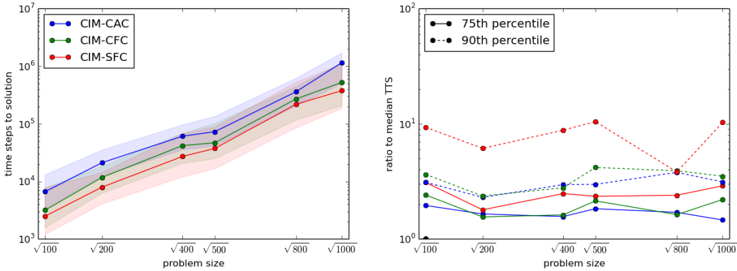<details> <summary>Image 10 Details</summary>  ### Visual Description ## Line Chart and Scatter Plot: Performance Analysis of CIM Methods ### Overview The image contains two side-by-side graphs analyzing the performance of three computational methods (CIM-CAC, CIM-CFC, CIM-SFC) across varying problem sizes. The left graph shows time steps to solution, while the right graph compares performance variability via percentile ratios. ### Components/Axes **Left Graph (Line Chart):** - **X-axis**: Problem size (√100 to √1000, logarithmic scale) - **Y-axis**: Time steps to solution (10³ to 10⁷, logarithmic scale) - **Legend**: - Blue: CIM-CAC - Green: CIM-CFC - Red: CIM-SFC - **Shaded Areas**: Confidence intervals (10% uncertainty) around each line **Right Graph (Scatter Plot):** - **X-axis**: Problem size (√100 to √1000, logarithmic scale) - **Y-axis**: Ratio to median TTS (10⁰ to 10², logarithmic scale) - **Legend**: - Solid dots: 75th percentile - Dashed dots: 90th percentile ### Detailed Analysis **Left Graph Trends:** 1. **CIM-CAC (Blue)**: - Starts at ~10³.5 steps at √100 - Rises to ~10⁶.5 steps at √1000 - Steepest slope among all methods 2. **CIM-CFC (Green)**: - Begins at ~10³.2 steps at √100 - Reaches ~10⁶ steps at √1000 - Slightly flatter than CIM-CAC 3. **CIM-SFC (Red)**: - Starts at ~10³ steps at √100 - Ends at ~10⁵.5 steps at √1000 - Most gradual increase **Right Graph Trends:** 1. **75th Percentile (Solid Dots)**: - Ranges from 0.5 to 5 across problem sizes - Peaks at √400 (3.2) and √800 (4.1) 2. **90th Percentile (Dashed Dots)**: - Ranges from 1 to 10 across problem sizes - Sharp peak at √1000 (10) - Dips below 1 at √200 (0.6) ### Key Observations 1. **Scalability**: All methods show exponential time growth with problem size, but CIM-SFC scales best (10⁵.5 vs 10⁶.5 for CIM-CAC at √1000). 2. **Variability**: - 90th percentile values are consistently 2-3x higher than 75th percentile - Largest variability occurs at √1000 (ratio reaches 10) 3. **Confidence Intervals**: Shaded areas in left graph widen by 40% between √400 and √1000, indicating increasing uncertainty. ### Interpretation The data demonstrates that: - **CIM-SFC** offers the most efficient scaling but with higher variability (wider shaded area) - **CIM-CAC** provides consistent performance but at a computational cost 10x higher than CIM-SFC at maximum problem size - The 90th percentile ratio suggests significant outlier cases in large problems, potentially indicating edge cases or hardware limitations - Logarithmic scaling reveals exponential growth patterns that would be less apparent in linear plots The shaded confidence intervals and percentile ratios together highlight a tradeoff between average performance and worst-case scenarios across different computational approaches. </details> ## 6.2 Comparison with noisy mean field annealing (NMFA) To show the importance of the auxiliary variable (error pulse) in CIM-SFC, we compared its performance to another CIM-inspired algorithm, namely noisy mean field annealing (NMFA). [ 26 ] NMFA also applies a hyperbolic tangent function to the mutual coupling term. However, it does not have an auxiliary variable and relies on (artificial) quantum noise to escape from local minima. Figure 11, compares the scal- ing of NMFA to CIM-SFC with different values of the feedback parameter k . As k controls the strength of the destabilization force caused by the auxiliary variable, we can measure the importance of the term k ( z i -e i ) to the scaling behavior. When k = 0, CIM-SFC is nearly identical to NMFA. The fact that CIM-SFC with k = 0 shows slightly worse performance indicates that the noise included in NMFA likely has a small effect and may help destabilize the local minima (which can also be observed in Figure 7). The case k = 0 . 15 is shown as an intermediate case, and k = 0 . 2 is the (experimentally obtained) optimal value for k in CIM-SFC. As can be seen, the addition of the error correction feedback term k ( z i -e i ) in Eq. (7) is effective in improving both the scaling and the spread of TTS for the SK instances. This implies that the 'correlated artificial noise' provided by the auxiliary variable is more effective in finding better solutions than the 'random quantum noise' from reservoirs. Figure 11: (left) TTSs of CIM-SFC and NMFA vs. problem size √ N . The shaded regions represent 25-75 percentile TTS. The results for NMFA are from [12]. (right) TTS for N=400 SK instances for different values of k . The 75th and 90th percentiles are not shown for smaller values of k because they were too large to be computed. 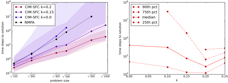<details> <summary>Image 11 Details</summary>  ### Visual Description ## Line Chart: Time Steps to Solution vs. Problem Size and Parameter k ### Overview The image contains two line charts comparing computational performance metrics across different problem sizes and parameter values. The left panel shows time steps to solution as a function of problem size for various algorithms, while the right panel displays time steps as a function of parameter k for percentile-based performance distributions. ### Components/Axes **Left Panel:** - **X-axis (Problem Size):** Logarithmic scale from √100 to √1000 (10 to 31.62 units) - **Y-axis (Time Steps to Solution):** Logarithmic scale from 10³ to 10⁸ - **Legend (Top-left):** - CIM-SFC k=0.2 (magenta circles) - CIM-SFC k=0.15 (purple circles) - CIM-SFC k=0.0 (blue circles) - NMFA (black dashed line with dots) - **Shaded Regions:** Confidence intervals around each line **Right Panel:** - **X-axis (k):** Linear scale from 0.00 to 0.25 - **Y-axis (Time Steps to Solution):** Logarithmic scale from 10⁴ to 10⁸ - **Legend (Top-right):** - 90th percentile (solid red line) - 75th percentile (dashed red line) - Median (dotted red line) - 25th percentile (dash-dot red line) ### Detailed Analysis **Left Panel Trends:** 1. **CIM-SFC k=0.2:** Starts at ~10³.5 steps at √100, rises to ~10⁵.5 at √1000 (magenta) 2. **CIM-SFC k=0.15:** Starts at ~10³.8, rises to ~10⁶ at √1000 (purple) 3. **CIM-SFC k=0.0:** Starts at ~10⁴, rises to ~10⁷ at √1000 (blue) 4. **NMFA:** Starts at ~10⁴, rises to ~10⁷.5 at √1000 (black dashed) - All lines show positive correlation between problem size and time steps - Confidence intervals widen with increasing problem size **Right Panel Trends:** - **90th percentile:** Starts at ~10⁷ at k=0.05, drops to ~10⁵ at k=0.15, then rises to ~10⁶ at k=0.25 - **75th percentile:** Starts at ~10⁶, drops to ~10⁴.5, then rises to ~10⁵.5 - **Median:** Starts at ~10⁵, drops to ~10⁴, then rises to ~10⁴.5 - **25th percentile:** Starts at ~10⁴, drops to ~10³.5, then rises to ~10⁴ ### Key Observations 1. **Algorithm Efficiency:** CIM-SFC with lower k values consistently outperforms NMFA across all problem sizes 2. **Scalability:** Time steps increase exponentially with problem size for all algorithms 3. **Parameter Sensitivity:** Right panel shows non-linear relationship between k and performance, with significant variance in upper percentiles 4. **Confidence Intervals:** Left panel shaded regions indicate increasing uncertainty with larger problem sizes ### Interpretation The data demonstrates that CIM-SFC algorithms with smaller k values (0.0-0.15) achieve better performance than NMFA, particularly at larger problem sizes. The right panel reveals that while median performance improves with increasing k, the 90th percentile shows a U-shaped pattern, suggesting some instances become significantly slower at extreme k values. This indicates that while average performance may improve with parameter tuning, there's a risk of outliers degrading results. The exponential scaling of time steps with problem size highlights the need for algorithmic optimizations to handle larger datasets efficiently. </details> ## 6.3 Comparison with discrete simulated bifurcation machine (dSBM) We compared the performance of the CIM-inspired algorithms with that of another heuristic Ising solver, namely the discrete simulated bifurcation machine (dSBM). [ 27 , 29 , 28 ] Similar to CIM, dSBM also makes use of analog spins and continuous dynamics to solve combinatorial optimization problems. We are aware that the authors of [29] seem to claim that dSBM is algorithmically superior to CIM-CAC by comparing the required number of MVMs to solution. Although the authors of [29] discussed the wall clock TTS of their implementations on many problem sets, when making the claim of algorithmic superiority, they only used the median TTS (in units of MVM) on SK instances for two problem sizes. In this section, we will provide a more detailed comparison of the three algorithms (CIM-CAC, CIM-CFC and CIM-SFC) with dSBM using MVM to solution (or equivalently, integration time steps to solution) as the performance metric. As mentioned before, this is a good comparison because all these algorithms will have MVM as the computational bottleneck when implemented on a digital platform. As discussed in Section 4, the computation of the Ising energy can be left until the end of the trajectory in most cases; thus, for this section, we will only consider the MVM involved in the computation of the mutual coupling term when calculating the MVM to solution. The problem instance sets used in this section are: 1. A set of 100 randomly generated 800-spin SK instances (available upon request from the authors). This instance set contains fully connected instances with weights of +1 , -1. 2. The G-set instances that have been used as a benchmark for max-cut performance (available at https://web.stanford.edu/ yyye/yyye/Gset/). In this study, we consider 50 instances with a problem size of 800-2000. These instances have varying edge density and include weights of either +1 , 0 or +1 , 0 , -1. 3. Another set of 1000 randomly generated 800-spin and 1200-spin SK instance (available upon request from the authors) used to evaluate the worst-case performance. To compare the performance on the 800-spin SK instances, the dSBM algorithm was also implemented on GPU. The parameters for dSBM were chosen on the basis of the parameters in [29] (see Appendix D). Figure 12: Required number of MVMs to solution for CIM-CAC, CIM-CFC, and CIM-SFC vs. that for dSBM. The median TTS is indicated by the red lines and the 25th-75th percentiles are indicated by the shaded blue regions. 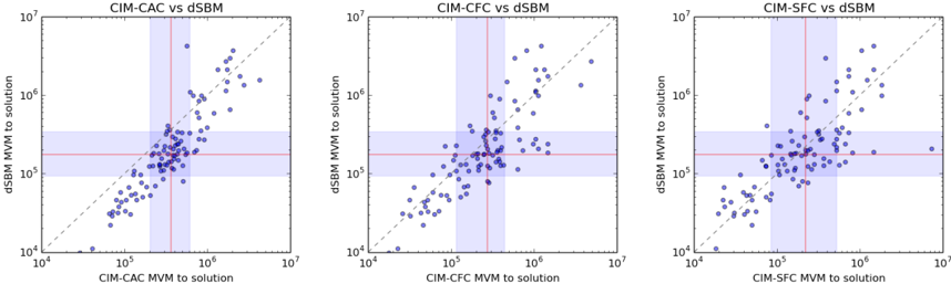<details> <summary>Image 12 Details</summary>  ### Visual Description ## Scatter Plots: CIM Methods vs dSBM Performance Comparison ### Overview Three scatter plots compare the Mean Value Metric (MVM) performance of different CIM (Circuit-Level Image Modeling) methods (CAC, CFC, SFC) against dSBM (Distributed Stochastic Block Model) across logarithmic scales. Each plot visualizes the relationship between CIM method performance and dSBM performance, with statistical reference lines and shaded regions. ### Components/Axes 1. **X-Axes (CIM Method to Solution)**: - Logarithmic scale from 10⁴ to 10⁷ - Labels: "CIM-CAC MVM to solution", "CIM-CFC MVM to solution", "CIM-SFC MVM to solution" 2. **Y-Axes (dSBM to Solution)**: - Logarithmic scale from 10⁴ to 10⁷ - Label: "dSBM MVM to solution" 3. **Visual Elements**: - **Dashed Line**: Diagonal line representing y = x (parity line) - **Shaded Regions**: - Vertical band (purple) centered at 10⁵–10⁶ - Horizontal band (pink) centered at 10⁵–10⁶ - **Data Points**: Blue dots representing individual measurements ### Detailed Analysis 1. **CIM-CAC vs dSBM**: - Data points cluster around the dashed line, indicating similar performance between CIM-CAC and dSBM. - Shaded regions suggest most data points fall within 10⁵–10⁶ for both axes. - Outliers: A few points deviate significantly (e.g., 10⁴–10⁵ on x-axis with y-axis >10⁶). 2. **CIM-CFC vs dSBM**: - Similar clustering pattern to CIM-CAC, with tighter alignment to the dashed line. - Shaded regions overlap with CIM-CAC, but fewer points exceed 10⁶ on either axis. 3. **CIM-SFC vs dSBM**: - Broader spread of data points, with some extending beyond 10⁶ on both axes. - Shaded regions remain consistent, but more points cluster near the lower bounds (10⁴–10⁵). ### Key Observations - **Consistency**: All three CIM methods show strong alignment with dSBM near the parity line (y = x), suggesting comparable performance in the 10⁵–10⁶ range. - **Variability**: CIM-SFC exhibits greater variability, with data points more dispersed across the log scale. - **Statistical Bands**: The shaded regions (10⁵–10⁶) likely represent confidence intervals or typical performance bounds, with most data points falling within these bounds. ### Interpretation The plots demonstrate that CIM methods (CAC, CFC, SFC) generally achieve performance comparable to dSBM, particularly in the mid-range (10⁵–10⁶). The shaded regions and dashed line serve as visual anchors for assessing agreement between methods. CIM-SFC shows the widest performance distribution, potentially indicating higher sensitivity to input variations or methodological differences. The absence of extreme outliers suggests robustness across methods, though CIM-SFC's broader spread warrants further investigation into its performance drivers. The logarithmic scale emphasizes relative differences, highlighting that performance gaps are more pronounced at the extremes (e.g., 10⁴ vs 10⁷). </details> In Figure 12compares the performance of the three algorithms (CIM-CAC, CIM-CFC, and CIM-SFC) instance by instance with that of dSBM on the 800-spin SK instance set. The ground-state energies used to evaluate the MVM to solution are the lowest energies found by the four algorithms. As all four algorithms found the same lowest energies, it is highly likely that these are true ground-state energies. The parameters for all four systems can be found in Appendix A. As shown in Figure 12, all four systems showed remarkably similar performance on the 800-spin instances when the parameters were optimized. It is important to note that with the parameters used in Figure 12, CIM-SFC did not find the ground state in one instance. However, if different parameters are used, CIM-SFC will find the ground state for this particular instance as well. Thus, although CIM-SFC can achieve high performance, it is highly sensitive to parameter selection. The median TTS (in the units of MVM) of CIM-CFC, CIM-SFC and dSBM are nearly the same: around 2 × 10 5 . Furthermore, the spread in TTS of these three algorithms is similar. Although CIM-CAC shows slightly worse median TTS (by less than a factor of two), it is worth noting that the instances in which CIM-CAC performs better than dSBM tend to be the harder instances. This indicates that among the four algorithms, CIM-CAC may show slightly better worst-case performance. We investigate this further later in this section. This pattern can also be seen on the G-set. Overall, all four algorithms show similar performance on the fully connected instance set, and it is impossible to determine which particular algorithm is the most effective one for this problem type. In addition to the similar median TTS and spread, there is a high level of correlation in the TTS among all four systems. This indicates either that instance difficulty is a universal property for all Ising heuristics or that there is something fundamentally common to the four algorithms. See Appendix E for a further discussion of the similarities and differences between these four systems. Although CIM-SFC shows good performance on fully connected problem instances, it struggles on many G-set instances. In Appendix D, we discuss a partial reason for this failure; however, the full reason is yet to be understood. In the future, we expect to modify CIM-SFC or find better parameters so that it can solve all problem types; however, for now, we will just consider CIM-SFC as a fully connected (or densely connected) Ising solver and compare only CIM-CAC, CIM-CFC, and dSBM on the G-set. For some results of CIM- SFC on the G-set, see Appendix D. All three algorithms (CIM-CAC, CIM-CFC, and dSBM) show fairly good performance on the G-set; however, we argue that CIM-CAC is the most consistently effective algorithm. CIM-CAC and dSBM Q Figure 13: (left) TTS on G-set graphs for CIM-CAC, CIM-CFC and dSBM. The best known cut values are found in [29]. The TTS for dSBM is from [29]. In this plot, the instances are separated into groups depending on the graph type and size. The dots above the plot indicate that the best known cut value was not found. (right) Histograms showing which algorithm realizes the slowest TTS and which algorithm has the fastest TTS. The column labeled 'none' indicates the two instances in which none of the three algorithms found the best known cut value. The parameters are chosen and optimized separately for each instance type. An instance-by-instance comparison and the parameters used are presented in Appendix B. 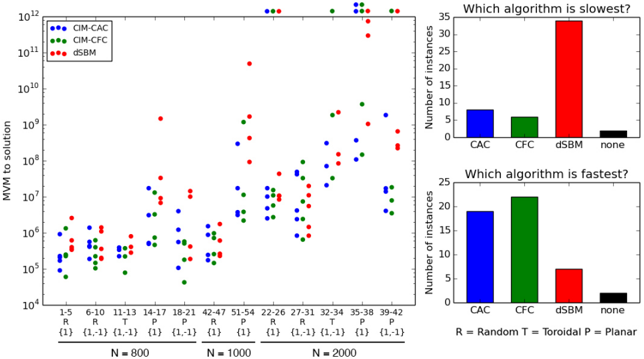<details> <summary>Image 13 Details</summary>  ### Visual Description ## Scatter Plot with Bar Charts: Algorithm Performance Analysis ### Overview The image presents a scatter plot comparing the Mean Maximum Value (MMV) to solution across different problem instances and algorithms, alongside two bar charts analyzing algorithm speed. The scatter plot uses three data series (CIM-CAC, CIM-CFC, dSBM) with varying problem sizes (N=800, 1000, 2000) and parameters (R=Random, T=Torroidal, P=Planar). The bar charts quantify algorithm performance extremes. ### Components/Axes **Main Scatter Plot**: - **X-axis**: Problem size (N=800, 1000, 2000) and parameter combinations (R, T, P). Labels include: - N=800: R, R, T, P, P - N=1000: R, T, P, P - N=2000: R, R, T, P, P - **Y-axis**: MMV to solution (log scale, 10⁴ to 10¹²). - **Legend**: Top-right, with: - Blue: CIM-CAC - Green: CIM-CFC - Red: dSBM **Bar Charts**: - **Top Chart**: "Which algorithm is slowest?" (Y-axis: Number of instances, 0–30). - **Bottom Chart**: "Which algorithm is fastest?" (Y-axis: Number of instances, 0–25). ### Detailed Analysis **Scatter Plot Trends**: - **CIM-CAC (Blue)**: Points cluster at lower MMV values (10⁵–10⁸) across all N and parameters. Notable outliers at N=2000 (R, T) with MMV ~10¹¹. - **CIM-CFC (Green)**: Distributed across mid-range MMV (10⁶–10⁹), with higher density at N=1000 (T, P). - **dSBM (Red)**: Scattered widely, with extreme values (e.g., N=2000, R: MMV ~10¹²; N=800, P: MMV ~10⁷). **Bar Chart Data**: - **Slowest Algorithm**: - dSBM: 30 instances (tallest red bar). - CAC: 8 instances (blue bar). - CFC: 5 instances (green bar). - "None": 1 instance (black bar). - **Fastest Algorithm**: - CAC: 18 instances (tallest blue bar). - CFC: 22 instances (green bar). - dSBM: 6 instances (red bar). - "None": 1 instance (black bar). ### Key Observations 1. **MMV Variability**: dSBM exhibits the highest MMV values (up to 10¹²), suggesting slower convergence or larger solution spaces. 2. **Algorithm Speed**: dSBM is the slowest (30 instances), while CAC is the fastest (18 instances). 3. **Parameter Impact**: Torroidal (T) and Planar (P) parameters correlate with higher MMV for dSBM, while Random (R) shows mixed results. 4. **Outliers**: CIM-CAC at N=2000 (R, T) has anomalously high MMV (~10¹¹), deviating from its typical range. ### Interpretation The data highlights significant differences in algorithm performance: - **dSBM** struggles with scalability, as evidenced by its dominance in the "slowest" category and extreme MMV values. This may stem from computational complexity or suboptimal parameter handling. - **CIM-CAC** demonstrates efficiency, achieving the lowest MMV and fastest execution. Its performance remains stable across problem sizes and parameters. - **CIM-CFC** offers moderate performance, with MMV values intermediate between CIM-CAC and dSBM. Its speed is second only to CAC. - The "None" category (1 instance each) suggests rare cases where no algorithm was applied or performed exceptionally. The scatter plot’s log scale emphasizes exponential differences in MMV, while the bar charts quantify algorithmic trade-offs. These results imply that algorithm selection should prioritize problem size, parameter structure, and computational constraints. </details> were able to find the best known cut values in 47 out of 50 instances, while CIM-CFC found the best known cut value in 45 out of 50 instances. It is worth noting that the simulation time used to calculate the TTS for dSBM [ 29 ] was much longer than that used in this study. Given the same simulation time, dSBM would most likely have solved only 45 out of 50 instances. As shown in Figure 13, CIM-CAC and CIM-CFC are faster (in units of MVM) than dSBM in most instances. More importantly, among the instances in which dSBM is faster, there are no cases where dSBM is significantly faster than CIM-CAC, other than G37, in which CIM-CAC did not find the best known cut value. Meanwhile, we found that CIM-CAC was more than an order of magnitude faster than dSBM in 13 out 50 instances. Therefore, we believe that CIM-CAC is a more reliable algorithm when considering many problem types. The difference between CIM-CAC and CIM-CFC is subtle. This is to be expected, as the dynamics of the two systems are very similar. Although the performance of the two algorithms for G-set is nearly identical in most cases, for some of the harder instances, there are some cases in which CIM-CFC cannot find the best known cut value or CIM-CFC has a significantly longer TTS. This indicates that CIMCAC is fundamentally a more promising algorithm or that precise parameter selection for CIM-CFC is required. As noted in Figure 12, the worst case performance of CIM-CAC may be slightly better than that of dSBM. To evaluate this further we created new sets of 1000 800-spin and 1200-spin SK instances. Figure 14 shows the number of instances solved as a function of the number of MVMs required to achieve a success probability of 99%. As can be seen in both cases, dSBM can solve the easier instances with fewer MVMs; however, for the hardest instances, CIM-CAC is faster. his can be understood by observing the intersection point of the two curves in Figure 14. In nearly all cases, the best Ising energy found was the same for both the solvers when a similar number of MVMs were used (see Appendix A for the parameters). However, for two instances in the N=1200 set, the Ising energy found by CAC was not found by dSBM. This remained true even when 50,000 dSBM trajectories were used for these instances. Our results suggest that dSBM may struggle considerably for some harder SK instances. However, we acknowledge that this could be a result of sub-optimal parameter selection for dSBM. 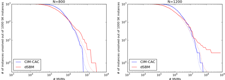The parameters used (see appendix A) were optimized manually to achieve a good median TTS; however, they may not <details> <summary>Image 14 Details</summary>  ### Visual Description ## Line Graph: Comparison of CIM-CAC and dSBM for Solving SK Instances ### Overview The image contains two side-by-side line graphs comparing the performance of two algorithms, **CIM-CAC** (blue) and **dSBM** (red), in solving **SK instances** for two different problem sizes: **N=800** (left graph) and **N=1200** (right graph). The y-axis represents the number of unresolved instances out of 1000 SK instances, while the x-axis represents the number of MVMs (Minimum Vertex Models). Both graphs show a logarithmic scale on both axes. --- ### Components/Axes - **X-axis (Horizontal)**: - Label: `# MVMs` (Minimum Vertex Models) - Scale: Logarithmic, ranging from **10³** to **10⁸**. - Ticks: Marked at **10³, 10⁴, 10⁵, 10⁶, 10⁷, 10⁸**. - **Y-axis (Vertical)**: - Label: `# instances unresolved out of 1000 SK instances` - Scale: Logarithmic, ranging from **10⁰** to **10³**. - Ticks: Marked at **10⁰, 10¹, 10², 10³**. - **Legend**: - Position: Bottom-left corner of both graphs. - Entries: - **Blue line**: CIM-CAC - **Red line**: dSBM - Additional elements: Dashed lines (possibly confidence intervals or error bounds, though not explicitly labeled). --- ### Detailed Analysis #### Left Graph (N=800) - **CIM-CAC (Blue)**: - Starts near **10³ unresolved instances** at **10³ MVMs**. - Declines sharply, reaching **~10¹ unresolved instances** by **10⁶ MVMs**. - Further decreases to **~10⁰ unresolved instances** by **10⁷ MVMs**. - The line is smooth and monotonically decreasing. - **dSBM (Red)**: - Starts near **10³ unresolved instances** at **10³ MVMs**. - Declines more gradually than CIM-CAC, reaching **~10¹ unresolved instances** by **10⁶ MVMs**. - Remains above CIM-CAC throughout, with a steeper drop after **10⁶ MVMs**. #### Right Graph (N=1200) - **CIM-CAC (Blue)**: - Starts near **10³ unresolved instances** at **10³ MVMs**. - Declines sharply, reaching **~10¹ unresolved instances** by **10⁶ MVMs**. - Further decreases to **~10⁰ unresolved instances** by **10⁷ MVMs**. - The line is smoother and more pronounced than in the N=800 case. - **dSBM (Red)**: - Starts near **10³ unresolved instances** at **10³ MVMs**. - Declines more gradually than CIM-CAC, reaching **~10¹ unresolved instances** by **10⁶ MVMs**. - Remains above CIM-CAC throughout, with a steeper drop after **10⁶ MVMs**. --- ### Key Observations 1. **CIM-CAC consistently outperforms dSBM** in both graphs, resolving more instances as the number of MVMs increases. 2. **Performance gap widens with larger N**: - For **N=1200**, CIM-CAC resolves instances at a faster rate than for **N=800**, especially beyond **10⁶ MVMs**. 3. **Dashed lines** (likely error bounds) show variability in the data, but the trends remain consistent. 4. **Logarithmic scaling** emphasizes the exponential decay of unresolved instances for both algorithms. --- ### Interpretation The data demonstrates that **CIM-CAC is significantly more efficient** than dSBM in solving SK instances, particularly for larger problem sizes (N=1200). The logarithmic scale highlights the exponential improvement in performance as MVMs increase. The dashed lines suggest that the results may have some variability, but the overall trend is clear. This implies that CIM-CAC could be a more scalable solution for large-scale SK problems, while dSBM may struggle with higher complexity. The graphs also indicate that the number of MVMs required to resolve instances grows exponentially with problem size, underscoring the computational challenges of SK instances. </details> # MVMs # MVMs Figure 14: Number of instances that remain unsolved (success probability under 99%) after a certain number of MVMs (time steps) for CIM-CAC and dSBM. The dotted lines represent the assumption of a log-normal distribution for the TTS on randomly generated SK instances. The instance sets used are 1000 randomly generated SK instances (different from the 100 instances used in Figure 12) of problem sizes N=800 (top) and N=1200 (bottom). The parameters for both systems can be found in Appendix A. be the best parameters if one wants to solve the hardest instances. By contrast, for CIM-CAC, the optimal parameters for the median TTS appear to also perform well on the hardest instances. To ensure that an Ising solver can find the true ground state of a given problem, the worst-case performance is very important. For this purpose, we believe that CIM-CAC is likely the more fundamentally superior algorithm, at least in the case of randomly generated SK instances. For the other CIM modifications, this is likely not true. In particular, for CIM-SFC, the worst-case performance is significantly worse than that of dSBM and CIM-CAC (as shown in Figure 10). In the future, it would be interesting to investigate the cause for this phenomenon and also to examine the spread of TTS for different problem types. ## 7 Conclusion The new coherent Ising machines presented in this paper (CIM-CFC and CIM-SFC) have considerable potential as both digital heuristic algorithms and optically implemented physical devices. Rapid advances in the thin-film LiNbO 3 platform [ 15 , 16 , 17 ] as a photonic integrated circuit technology might enable the proposed optical CIM to surpass existing digital algorithms on a CMOS platform in terms of both speed and energy consumption. The proposed CIM-inspired algorithms were shown to be fast and accurate Ising solvers even when implemented on an existing digital platform. In particular, we showed that their performance is very similar to that of other existing analog-system-based algorithms such as dSBM. This again brings up the question raised in [11] as to whether the simulation of analog spins on a digital computer can outperform a purely discrete heuristic algorithm. Finally, whether chaotic dynamics are necessary for a deterministic dynamical system to be a good Ising solver is left as an open issue for future research. [ 11 , 12 , 29 ] ## Appendix A: Optimization of simulation parameters Here we summarize the simulation parameters used in our numerical experiments. The parameters are optimized empirically and thus do not necessarily reflect the true optimum values. ## Parameters used in Figure 5 | N step | CIM-SFC (upper left panel) | | CIM-CFC (upper right panel) | |----------|------------------------------|--------|-------------------------------| | | 500 | N step | 1000 | | ∆ T | 0.4 | ∆ T | 0.4 | | p | -1.0 | p | -1.0 | | c | 1.0 | α | 1.0 | | β | 0.3 | β | | | k | 0.2 | | 0.2 | | | CIM-SFC (lower left panel) | | CIM-CFC (lower right panel) | | | | N step | 1000 | | N step | 500 | ∆ T | 0.4 | | ∆ T | 0.4 | T | 900 | | p | -1.0 → 1.0 | r T | 100 | | c | 1.0 → 3.0 | p | | | β | 0.3 → 0.1 | p | -1.0 → 1.0 | | | | α | 1.0 | | k | 0.2 | β | 0.2 | ## Parameters used in Figure 10, 11, and 12 ## CIM-CAC In our simulation, the x i variables are restricted to the range [ -3 2 √ α, 3 2 √ α ] at each time step. The parameters p and α are modulated linearly from their starting to ending values during the T r time steps and are kept at the final value for an additional T p time steps. The initial value x i is set to a random value chosen from a zero-mean Gaussian distribution with a standard deviation of 10 -4 and e i = 1. Furthermore, 3200 trajectories are computed per instance to evaluate TTS. The actual parameters used for simulation are listed below: | N step | 3200 | |----------|------------| | ∆ T | 0.125 | | T r | 2880 | | T p | 320 | | p | -1.0 → 1.0 | | α | 1.0 → 2.5 | | β | 0.8 | ## CIM-CFC In our simulation the x i variables are restricted to the range [ -1 . 5 , 1 . 5] and e i is restricted to the range [0 . 01 , ∞ ]. The parameter p is modulated linearly from its starting to ending values during the first T r time steps and kept at the final value for an additional T p time steps. The initial value x i is set to a random value chosen from a zero-mean Gaussian distribution with a standard deviation of 0 . 1 and e i = 1. Furthermore, 3200 trajectories are computed per instance to evaluate TTS. The actual parameters used for simulation are listed below: | N step | 1000 | |----------|------------| | ∆ T | 0.4 | | T r | 900 | | T p | 100 | | p | -1.0 → 1.0 | | α | 1.0 | | β | 0.2 | ## CIM-SFC Restriction of x i and e i variables is not needed as this system is more numerically stable. The parameters p , c and β are modulated linearly from their starting to ending values during simulation. The initial value x i is set to a random value chosen from a zero-mean Gaussian distribution with standard deviation of 0 . 1 and e i = 0. 3200 trajectories are computed per instance to evaluate TTS. Actual parameters used for simulation are listed below: | N step | 500 | |----------|------------| | ∆ T | 0.4 | | p | -1.0 → 1.0 | | c | 1.0 → 3.0 | | β | 0.3 → 0.1 | | k | 0.2 | In addition to the above-mentioned parameters, it is important for the normalizing factor ξ for the mutual coupling term to be chosen as [31], $$\xi = \sqrt { \frac { 2 N } { \sum J _ { i j } ^ { 2 } } } .$$ This choice is crucial for the successful performance of CIM-SFC but not for CIM-CAC and CIM-CFC. Moreover, it is important to note that we used the same number of time steps for all the problem sizes in Figures 10 and 11. It is likely that the optimal number of time steps is smaller for smaller problem sizes, thus the scaling of TTS when the number of time steps is optimized separately for each problem size might be slightly worse than the reported scaling. However, we do not believe that this difference would be very significant. For the scaling of TTS for CIM-CAC when different parameters are chosen, see Appendix C. ## dSBM For Figure 12, dSBM is implemented as described in [29]. The parameters used are $$\frac { N \text { step} } { \Delta T } & = 2 0 0 0 \\ c & = 0 . 5$$ ## Parameters used in Figure 14 The parameters for N=800 are the same as those for Figure 12. The parameters for N=1200 are listed below. The number of trajectories used for N=1200 was 3200 for most instances; however, to accurately evaluate the success probability, 10000-50000 trajectories were computed for the 10 hardest instances for both algorithms. Moreover, owing to the hardness in the case of N=1200, we are not very certain that the true ground state was found. ## CIM-CAC | N step | 8000 | |----------|------------| | ∆ T | 0.125 | | T r | 7200 | | T p | 800 | | p | -1.0 → 1.0 | | α | 1.0 → 2.5 | | β | 0.8 | ## dSBM ## Numerical Integration An Euler step is used for integration in all the cases (except for dSBM). As described above we constrain the range of x i variables to ensure numerical stability. This is not necessary for performance but allows us to increase the integration time step by a factor of 2 or 3 without compromising the success probability. In Figure 15 we show the success probability of CIM-CAC with respect to the time step for both constrained and unconstrained systems. The results in Section 5 for CIM-CFC do not use this numerical constraint the CIM in Section 5 is meant to be a physical machine, and a time step of 0.2 is used. ## Appendix B: Simulation Results for G-set The results in Figure 13 for dSBM are taken directly from the GPU implementation of dSBM in [29]. The unit for TTS in Table ?? is time steps to solution, or equivalently, MVM to solution. In our simulation, 3200, 10000, or 32000 trajectories were generated to evaluate the TTS depending on the instance difficulty. The numbers in bold denote the best TTS among the three algorithms. Figure 15: Success probability of CIM-CAC with respect to time step for both constrained and unconstrained systems. For the blue curve, the x i amplitudes are restricted to the range [ -1 . 5 √ α, 1 . 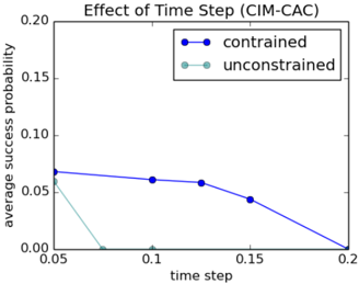5 √ α ] <details> <summary>Image 15 Details</summary>  ### Visual Description ## Line Graph: Effect of Time Step (CIM-CAC) ### Overview The image is a line graph illustrating how the **average success probability** changes with varying **time step** values in a system labeled "CIM-CAC". Two data series are compared: "constrained" (blue line) and "unconstrained" (green line). The graph shows a clear divergence in trends between the two scenarios as the time step increases. --- ### Components/Axes - **Title**: "Effect of Time Step (CIM-CAC)" - **X-axis**: - Label: "time step" - Scale: 0.05 to 0.2 (increments of 0.05) - **Y-axis**: - Label: "average success probability" - Scale: 0.00 to 0.20 (increments of 0.05) - **Legend**: - Position: Top-right corner - Entries: - "constrained" (blue line with circular markers) - "unconstrained" (green line with circular markers) --- ### Detailed Analysis #### Constrained (Blue Line) - **Trend**: Gradual decline from left to right. - **Data Points**: - At time step 0.05: ~0.06 - At time step 0.1: ~0.055 - At time step 0.15: ~0.045 - At time step 0.2: 0.00 #### Unconstrained (Green Line) - **Trend**: Sharp initial drop, then plateaus at 0.00. - **Data Points**: - At time step 0.05: ~0.05 - At time step 0.075: 0.00 (drops sharply) - Remains at 0.00 for all subsequent time steps (0.1, 0.15, 0.2). --- ### Key Observations 1. **Constrained System**: - Success probability decreases linearly with increasing time step. - Maintains non-zero probability until the maximum time step (0.2). 2. **Unconstrained System**: - Success probability drops abruptly at time step 0.075 and remains at 0.00 for all larger time steps. - Initial success probability (~0.05) is slightly lower than the constrained system at the same time step. 3. **Divergence**: - The constrained system retains higher success probability across most time steps. - The unconstrained system’s success probability collapses earlier, suggesting sensitivity to time step changes. --- ### Interpretation The data suggests that **time step size critically impacts system performance**, with the **constrained scenario** being more robust to increases in time step. The unconstrained system’s rapid decline in success probability implies that it may lack mechanisms (e.g., feedback, regulation) to adapt to larger time steps, leading to failure. This could reflect a trade-off between computational efficiency (larger time steps) and stability (smaller time steps). The constrained system’s gradual decline might indicate controlled adjustments to maintain functionality, whereas the unconstrained system’s abrupt failure highlights vulnerabilities in its design or parameters. The graph underscores the importance of time step selection in dynamic systems, particularly when balancing performance and computational constraints. </details> ## CIM-CAC parameters for G-set The variables are restricted as described in Appendix A, and the initial conditions are set in the same way. The following parameters are the same for all the G-set instances. $$\frac { \alpha } { \beta } | \begin{array} { c | c } 1 . 0 & 3 . 0 \\ 0 . 3 \end{array}$$ The parameters p , ∆ T , and the number of time steps used in each phase are chosen by instance type as follows: | N step | 4000 | |----------|--------| | ∆ T | 1.25 | | c | 0.5 | | Graph Type | Edge Weight | N | Instance # | p | N step | ∆ T | T r | T p | |--------------|---------------|------|--------------|-------------|----------|-------|-------|-------| | Random | { +1 } | 800 | 1-5 | -0.5 → 1.0 | 6666 | 0.075 | 6000 | 666 | | Random | { +1, -1 } | 800 | 6-10 | -0.5 → 1.0 | 6666 | 0.075 | 6000 | 666 | | Toroidal | { +1, -1 } | 800 | 11-13 | -4.0 | 5000 | 0.1 | 4500 | 500 | | Planar | { +1 } | 800 | 14-17 | -1.0 | 20000 | 0.05 | 18000 | 2000 | | Planar | { +1, -1 } | 800 | 18-21 | -1.0 | 20000 | 0.05 | 18000 | 2000 | | Random | { +1 } | 1000 | 43-46 | -0.5 → 1.0 | 10000 | 0.1 | 9000 | 1000 | | Planar | { +1 } | 1000 | 51-54 | -1.0 | 20000 | 0.05 | 18000 | 2000 | | Random | { +1 } | 2000 | 22-26 | -0.5 → 1.0 | 20000 | 0.1 | 19000 | 1000 | | Random | { +1, -1 } | 2000 | 27-31 | -0.5 → 1.0 | 20000 | 0.1 | 19000 | 1000 | | Toroidal | { +1, -1 } | 2000 | 32-34 | -4.0 → -3.0 | 20000 | 0.1 | 19000 | 1000 | | Planar | { +1 } | 2000 | 35-38 | -1.0 → -0.5 | 80000 | 0.05 | 78000 | 2000 | | Planar | { +1 } | 2000 | 39-42 | -1.0 → -0.5 | 80000 | 0.05 | 78000 | 2000 | ## CIM-CFC parameters for G-set The variables are restricted as described in Appendix A, and the initial conditions are set in the same way. The following parameters are the same for all the G-set instances. $$\frac { \alpha } { \beta } \left | \begin{array} { c c } { 1 . 0 } \\ { 0 . 1 5 } \end{array} \right |$$ The parameters p , ∆ T , and the number of time steps used in each phase are chosen by instance type as follows: | Graph Type | Edge Weight | N | Instance # | p | N step | ∆ T | T r | T p | |--------------|---------------|------|--------------|-------------|----------|-------|-------|-------| | Random | { +1 } | 800 | 1-5 | -1.0 → 1.0 | 4000 | 0.125 | 3600 | 400 | | Random | { +1, -1 } | 800 | 6-10 | -1.0 → 1.0 | 2000 | 0.25 | 1800 | 200 | | Toroidal | { +1, -1 } | 800 | 11-13 | -3.0 → -1.0 | 2000 | 0.25 | 1800 | 200 | | Planar | { +1 } | 800 | 14-17 | -2.0 → 0.0 | 8000 | 0.125 | 7200 | 800 | | Planar | { +1, -1 } | 800 | 18-21 | -2.0 → 0.0 | 4000 | 0.25 | 3600 | 400 | | Random | { +1 } | 1000 | 43-46 | -1.0 → 1.0 | 5000 | 0.2 | 4500 | 500 | | Planar | { +1 } | 1000 | 51-54 | -2.0 → 0.0 | 16000 | 0.125 | 15200 | 800 | | Random | { +1 } | 2000 | 22-26 | -1.0 → 1.0 | 10000 | 0.2 | 9500 | 500 | | Random | { +1, -1 } | 2000 | 27-31 | -1.0 → 1.0 | 10000 | 0.2 | 9500 | 500 | | Toroidal | { +1, -1 } | 2000 | 32-34 | -3.0 → -1.0 | 40000 | 0.1 | 39000 | 1000 | | Planar | { +1 } | 2000 | 35-38 | -2.0 → 0.0 | 80000 | 0.05 | 78000 | 2000 | | Planar | { +1 } | 2000 | 39-42 | -2.0 → 0.0 | 40000 | 0.1 | 39000 | 1000 | ## Results on G-set Success probability and TTS of CIM-CAC, CIM-CFC and dSBM on G-set graphs. The success probability for CIM-CAC and CIM-CFC is for a single trajectory. The results for dSBM are from the GPU implementation in [29]. | Instance | CIM-CAC TTS | CIM-CAC P s | CIM-CFC TTS | CIM-CFC P s | dSBM TTS | dSBM P s * | |------------|--------------------|---------------|---------------|---------------|---------------------|--------------| | G1 | 90805 | 0.286875 | 60078 | 0.264062 | 339332 | 0.987 | | G2 | 920217 | 0.0328125 | 1330454 | 0.01375 | 2578124 | 0.82 | | G3 | 169551 | 0.165625 | 249212 | 0.07125 | 400343 | 0.996 | | G4 | 209086 | 0.136563 | 239389 | 0.0740625 | 361673 | 0.983 | | G5 | 226881 | 0.126562 | 226449 | 0.078125 | 618221 | 0.972 | | G6 | 188908 | 0.15 | 104083 | 0.0846875 | 190728 | 0.979 | | G7 | 562413 | 0.053125 | 146490 | 0.0609375 | 201889 | 0.974 | | G8 | 431029 | 0.06875 | 399118 | 0.0228125 | 358947 | 0.954 | | G9 | 411604 | 0.071875 | 223836 | 0.0403125 | 1095704 | 0.867 | | G10 | 1388073 | 0.021875 | 622470 | 0.0146875 | 1410031 | 0.407 | | G11 | 337563 | 0.0659375 | 222079 | 0.040625 | 282524 | 0.98 | | G12 | 224452 | 0.0975 | 78562 | 0.110625 | 407997 | 0.973 | | G13 | 391011 | 0.0571875 | 373236 | 0.024375 | 800687 | 0.996 | | G14 | 17291018 | 0.0053125 | 13080721 | 0.0028125 | 1469967245 | 0.005 | | G15 | 521572 | 0.161875 | 462528 | 0.0765625 | 6782113 | 0.804 | | G16 | 494303 | 0.17 | 737146 | 0.04875 | 9156329 | 0.992 | | G17 | 3089154 | 0.029375 | 3256332 | 0.01125 | 33222397 | 0.283 | | G18 | 556635 | 0.1525 | 507805 | 0.035625 | 14375986 | 0.074 | | G19 | 1218307 | 0.0728125 | 179562 | 0.0975 | 417204 | 0.995 | | G20 | 106718 | 0.578125 | 42428 | 0.352187 | 188349 | 0.98 | | G21 | 3991180 | 0.0228125 | 574365 | 0.0315625 | 10080921 | 0.136 | | G43 | 174031 | 0.2325 | 145625 | 0.14625 | 228908 | 0.992 | | G44 | 244188 | 0.171875 | 257230 | 0.085625 | 263171 | 0.985 | | G45 | 880856 | 0.0509375 | 970877 | 0.0234375 | 1754473 | 0.985 | | G46 | 1528073 | 0.0296875 | 717957 | 0.0315625 | 610421 | 0.992 | | G51 | 3732360 | 0.024375 | 2189016 | 0.0331 | 424989992 | 0.067 | | G52 | 3122871 | 0.0290625 | 3820774 | 0.0191 | 92285270 | 0.213 | | G53 | 17291018 | 0.0053125 | 11298922 | 0.0065 | 1676440469 | 0.043 | | G54 | 294684837 | 0.0003125 | 1178886725 | 6.25e-05 | 49107077298 | 0.0006 | | G22 | 2516544 | 0.0359375 | 2718081 | 0.0168 | 8401394 | 0.928 | | G23 | N/A | 0.0 | N/A | 0.0 | N/A | 0 | | G24 | 4785454 | 0.0190625 | 5733406 | 0.008 | 10585339 | 0.648 | | G25 | 17291018 | 0.0053125 | 15327529 | 0.003 | 43414254 | 0.399 | | G26 | 10117012 | 0.0090625 | 10941648 | 0.0042 | 10730290 | 0.643 | | G27 | 835530 | 0.104375 | 649972 | 0.0684 | 832465 | 0.971 | | G28 | 2389444 | 0.0378125 | 2413498 | 0.0189 | 1455914 | 0.952 | | G29 | 4164219 | 0.021875 | 7404644 | 0.0062 | 5516820 | 0.737 | | G30 | 42058344 | 0.0021875 | 32871041 | 0.0014 | 11002259 | 0.738 | | G31 | 49075749 | 0.001875 | 92080375 | 0.0005 | 19923732 | 0.199 | | G32 | 70802710 | 0.0013 | 1841975969 | 0.0001 | 150969342 | 0.093 | | G33 | 306965291 | 0.0003 | N/A | 0.0 | 2204950868 | 0.005 | | G34 | 20886506 | 0.0044 | 32801883 | 0.0056 | 84156149 | 0.231 | | G35 | N/A | 0.0 | N/A | 0.0 | N/A | 0 | | G36 | 368321503 | 0.0005 | 3683951938 | 0.0001 | 736790387782 | 0.0001 | | G38 | 108264816 | 0.0017 | | 0.0025 | 1046295719 | 0.068 | | | | | 147181162 | | | 0.107 | | G39 | 4065368 1841975969 | 0.0443 0.0001 | 3497864 N/A | 0.0513 0.0 | 651087484 264354894 | 0.154 | | G40 G41 | 17123320 | 0.0107 | 7916531 | 0.023 | 222414431 | 0.282 | | G42 | 13969282 | 0.0131 | 18328423 | 0.01 | N/A | 0 | *Note that P s for dSBM taken from [29] is the success probability for a batch of 160 trajectories. To calculate the P s for a single dSBM trajectory use 1 -(1 -P s ) 1 160 . ## Appendix C: Reasoning for parameter selection The parameters are selected numerically for the most part; however, the choice of p , α , and β can be understood as follows. It is observed that the average residual energy visited by CIM-CAC during the search process can be roughly estimated by the formula. [ 11 ] $$\Delta E _ { a v g } \approx K \frac { 1 - p } { \alpha \beta }$$ where K is a constant depending only on the problem type and size. This formula essentially predicts the effective sampling temperature of the system (although the distribution may not be an exact Boltzmann distribution). Based on this philosophy, we gradually reduce the 'system temperature' to produce an annealing effect. This is the motivation for increasing p and α . The different choices for the range of p on different G-set instances reflects the vastly different values for the constant K depending on the structure of the max-cut problem. In a more general setting, the value of K can be predicted on the basis of the problem type; thus, the range for p and α can be chosen accordingly. Although it has not been verified, a similar formula most likely holds for CIM-CFC; thus, the parameters for CIM-CFC are chosen in the same way. ## Optimal parameters with respect to problem size (CIM-CAC) Figure 16: Performance of CIM-CAC with respect to problem size for different parameters. The fixed parameters are indicated in red while the parameter modulation is indicated in blue. 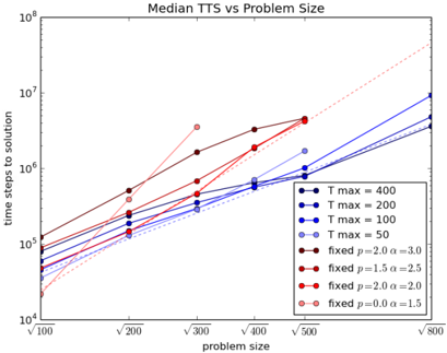The red and blue dotted lines are fits for the lower envelopes of the red and blue curves, respectively <details> <summary>Image 16 Details</summary>  ### Visual Description ## Line Chart: Median TTS vs Problem Size ### Overview The chart compares the median time-to-solution (TTS) across varying problem sizes (x-axis) for different configurations of a system. The y-axis represents time steps to solution on a logarithmic scale (10⁴ to 10⁸). Multiple data series are plotted, differentiated by T max values and fixed parameters (p, α). ### Components/Axes - **X-axis (Problem Size)**: Logarithmic scale with values √100, √200, √300, √400, √500, √800. - **Y-axis (Time Steps to Solution)**: Logarithmic scale from 10⁴ to 10⁸. - **Legend**: Located in the bottom-right corner, with 7 data series: - **T max = 400** (dark blue, circles) - **T max = 200** (blue, squares) - **T max = 100** (light blue, triangles) - **T max = 50** (dashed blue, diamonds) - **Fixed p=2.0 α=3.0** (brown, solid line) - **Fixed p=1.5 α=2.5** (red, solid line) - **Fixed p=2.0 α=2.0** (dark red, dashed line) - **Fixed p=0.0 α=1.5** (pink, dotted line) ### Detailed Analysis 1. **T max Series**: - **T max = 400** (dark blue): Steepest upward slope, reaching ~10⁷ at √500 and ~10⁸ at √800. - **T max = 200** (blue): Slower growth than T max = 400, ~10⁶ at √500, ~10⁷ at √800. - **T max = 100** (light blue): ~10⁵ at √500, ~10⁶ at √800. - **T max = 50** (dashed blue): ~10⁴ at √500, ~10⁵ at √800. 2. **Fixed Parameters Series**: - **p=2.0 α=3.0** (brown): ~10⁵ at √500, ~10⁶ at √800. - **p=1.5 α=2.5** (red): ~10⁶ at √500, ~10⁷ at √800. - **p=2.0 α=2.0** (dark red): ~10⁵ at √500, ~10⁶ at √800. - **p=0.0 α=1.5** (pink): Steepest slope, ~10⁶ at √500, ~10⁸ at √800. ### Key Observations - **Inverse Relationship**: Higher T max values correlate with longer time steps to solution. - **Fixed Parameters Impact**: Lower p and α values (e.g., p=0.0 α=1.5) result in significantly steeper growth curves. - **Outliers**: The pink dotted line (p=0.0 α=1.5) diverges sharply from other series, suggesting extreme sensitivity to these parameters. ### Interpretation The data demonstrates that system efficiency degrades with larger problem sizes, particularly under high T max settings. Fixed parameters (p, α) critically influence scalability: lower values (e.g., p=0.0) exacerbate time-step growth, while higher values (e.g., p=2.0 α=3.0) mitigate it. This suggests optimizing p and α is crucial for managing computational load in large-scale problems. The T max parameter acts as a tunable threshold, with higher values amplifying the system's resource demands. </details> Figure 16 shows the difference in scaling when the parameters are fixed (red shades) compared to when the parameters are modulated linearly (blue shades). In addition, the optimal annealing time (in other words, the optimal speed of modulation) will change with respect to the problem size, as we need long annealing times to get good results for large problem sizes. This pattern was also used when choosing parameters on the G-set. Although Figure 16 is based on the Gaussian quantum model for CIM-CAC in MFB-CIM (see [31]), the difference in performance between this model and the noiseless model discussed in this paper is insignificant, as g 2 = 10 -4 was used. It should also be noted that a time step of 0.01 was used in Figure 16. Therefore, the TTS in Figure 16 is an order of magnitude longer than the results presented in this study, where a time step of 0.125 was used. ## Appendix D: Results and Discussion for CIM-SFC on G-set Based on our understanding of CIM-SFC, it is very important that the term tanh( cz i ) transitions from the 'soft spin' mode where cz i ≈ 0 and tanh( cz i ) ≈ cz i to the 'discrete spin' mode where | cz i | >> 0 and tanh( cz i ) ≈ sign( cz i ). Therefore, we use the normalizing factor ξ (as defined above) as this ensures that z i will on average be around √ 2 for a randomly chosen spin configuration, thus we can use the same value for c in all the cases and get similar results. However, this only works for instances such as SK instances where each node has equal connectivity; thus, we can expect z i to have roughly the same range of values for all i . On some G-set instances, especially the planar graph instances, some nodes have a much larger degree; thus, cz i will be too large in some cases and too small in others regardless of the normalizing factor ξ used. This may be one of the reasons why CIM-SFC struggles on many G-set instances, especially planar graphs. This could also be the reason why dSBM struggles on planar graphs, as dSBM relies on the same normalizing factor to get good results. CIM-CAC and CIM-CFC do not need this normalizing factor, as they automatically compensate for different values of ∑ j J ij σ j , and this might be why they perform well on planar graphs. Meanwhile, for toroidal graphs, the opposite is true, as ∑ j J ij σ j can only take on five different values for these graphs. This could mean that the transition from 'soft spin' to 'discrete spin' is rapid in the case of CIM-SFC; thus, we need to carefully tune the parameters to get good results on these graphs. Although this observation regarding the analog/discrete transition may partially explain the poor results on the G-set, it is not a complete explanation. For example, CIM-SFC struggles on some random graphs (such as G9) that do not have the above-mentioned property, as each node has similar connectivity. The results for CIM-SFC on the G-set as well as the parameters used are listed below (not all instances were tested). ## Results for CIM-SFC on the G-set | Instance | TTS | P s | |------------|----------|-----------| | G1 | 28470 | 0.194 | | G2 | 1531984 | 0.004 | | G3 | 130388 | 0.046 | | G4 | 435510 | 0.014 | | G5 | 380685 | 0.016 | | G6 | 112834 | 0.0202 | | G7 | 163316 | 0.014 | | G8 | 125360 | 0.0182 | | G9 | 4604018 | 0.0005 | | G10 | 395845 | 0.0058 | | G11 | 195461 | 0.0572 | | G12 | 128184 | 0.0859 | | G13 | 311368 | 0.0363 | | G43 | 1702012 | 0.0134375 | | G44 | 1742812 | 0.013125 | | G45 | 73671209 | 0.0003125 | | G46 | 1927483 | 0.011875 | For instances G14-G21 (800 node planar graphs) and G51-G54 (1000 node planar graphs), CIM-SFC shows a success probability of either zero or a very small nonzero value. Furthermore, 2000 node instances have not been tested. ## Parameters for CIM-SFC on G-set ## Common parameters Parameters selected by problem type | Graph Type | Edge Weight | N | Instance # | c | β | k | N step | ∆ T | |--------------|---------------|------|--------------|-----------|------------|------|----------|-------| | Random | { +1 } | 800 | 1-5 | 1.0 → 3.0 | 0.3 → 0.0 | 0.2 | 2666 | 0.15 | | Random | { +1, -1 } | 800 | 6-10 | 1.0 → 3.0 | 0.3 → 0.0 | 0.2 | 500 | 0.4 | | Toroidal | { +1, -1 } | 800 | 11-13 | 1.4 | 0.05 → 0.0 | 0.32 | 2500 | 0.4 | | Random | { +1 } | 1000 | 43-46 | 1.4 → 4.2 | 0.2 → 0.0 | 0.2 | 5000 | 0.2 | The parameters for CIM-SFC are chosen experimentally, and the understanding of how the parameters affect the performance and dynamics is limited. Once this system is studied more thoroughly, we will propose a more systematic method of choosing parameters so that good performance can be ensured on many different problem types. ## Appendix E: Similarities and Differences Between CIM and SBM Algorithms Using continuous analog dynamics to solve discrete optimization problems is a somewhat new concept, and it is interesting to compare these different approaches. [ 13 , 11 , 29 ] In this appendix, we will briefly discuss some similarities and differences among the three CIM-inspired algorithms and the SBM algorithms. All four systems discussed in Section 6, namely CIM-CAC, CIM-CAC, CIM-SFC, and dSBM, were originally inspired by the same fundamental principle:[10, 27]: The function $$H ( x ) = \sum _ { i } \left ( \frac { x _ { i } ^ { 2 } } { 4 } - \frac { 1 - p } { 2 } \right ) x _ { i } ^ { 2 } + c \sum _ { i } \sum _ { j } J _ { i j } x _ { i } x _ { j }$$ can be used as a continuous approximation of the Ising cost function. In the original CIM algorithm, gradient descent is used to find the local minima of H , while H is deformed by increasing p . This system has two major drawbacks:[10] 1. local minima are stable; 2. incorrect mapping of the Ising problem to the cost function owing to amplitude heterogeneity. All four algorithms discussed in Section 6 can be regarded as modifications of the original CIM algorithm, which aim to overcome these two flaws. [ 11 , 27 , 28 , 29 ] In all these algorithms, the first flaw is addressed by adding new degrees of freedom to the system; hence, there are now 2 N (instead of only N ) analog variables for N spins. In SBM, this is done by including both a position vector, x i , and a velocity/momentum vector y i , while in the modified CIM algorithms we add the auxiliary variable e i . To address the second flaw, the creators of dSBM added discretization and 'inelastic walls', whereas in CIM- CFC and CIM-SFC, this discretization is not necessary. Using different mechanisms, all three algorithms ensure that the system only has fixed points at the local minima of the Ising Hamiltonian (during the end of the trajectory), something which is not true for the original CIM algorithm. Because these systems are fundamentally very similar, it should not be surprising that they achieve similar performance. $$p \, - 1 . 0 \to 1 . 0$$ We also note that for dSBM to achieve good performance, it is necessary to use discretization and inelastic walls, which make the system discontinuous. This is particularly useful for implementation on a digital platform, which prefers discrete processes; however, when implementing these algorithms on an analog physical platform, this is not preferred. Meanwhile, in the case of CIM-CAC, CIM-CFC, and CIM-SFC, the system evolves continuously; thus, they are much more suitable for analog implementation, such as the optical CIM architecture proposed in this paper. An interesting difference between the CIM and the original bifurcation machine [ 27 ] , which was referred to as aSBM in [29], is that aSBM is a completely unitary dissipation-less system. Because of this, aSBM relies on adiabatic evolution for computation (similar to quantum annealing), unlike the dissipative CIM and other Ising heuristics (such as simulated annealing or breakout local search [ 14 ] ) , which rely on some sort of dissipative relaxation. However, in [29], the new SBM algorithms deviate from this concept of adiabatic evolution by adding inelastic walls, thus making the new bifurcation machine a dissipative system in which information is lost over time. It would be interesting to try to understand whether dissipation is in fact necessary for a system to achieve the high performance of the algorithms discussed in this paper. For example, one could modify aSBM in a different way that addresses the problem of amplitude heterogeneity but retains the adiabatic nature. Whether this is possible is beyond the scope of this paper. ## Appendix F: Optical Implementation of CIM-SFC Figure 17: Optical implementation of CIM-SFC. 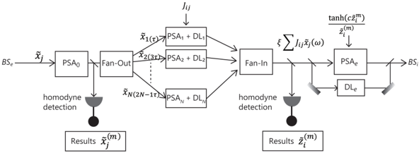<details> <summary>Image 17 Details</summary>  ### Visual Description ## Block Diagram: Quantum Signal Processing System ### Overview The diagram illustrates a multi-stage quantum signal processing system with parallel and sequential components. It features beam splitters (BS), parametric signal amplifiers (PSA), detectors (DL), fan-out/fan-in networks, and homodyne detection blocks. Mathematical operations and signal transformations are explicitly labeled. ### Components/Axes 1. **Input/Output Ports**: - Left: `BS_e` (input), `BS_i` (output) - Right: `BS_e` (input), `BS_i` (output) 2. **Core Components**: - `PSA_0` (initial parametric amplifier) - `Fan-Out` (signal splitting) - `PSA_1...PSA_N` (parametric amplifiers) - `DL_1...DL_N` (detectors) - `Fan-In` (signal recombination) - `PSA_e` (final parametric amplifier) - `DL_e` (final detector) 3. **Mathematical Labels**: - `J_ij`: Coupling coefficients between stages - `ξΣJ_ijx_j(ω)`: Summation of weighted signal components - `tanh(cz_i^m)`: Nonlinear transformation in final stage 4. **Detection Blocks**: - Homodyne detection (left and right sides) - Results labeled `x̃_j^(m)` and `z̃_i^(m)` ### Detailed Analysis - **Left Path**: 1. `BS_e` → `PSA_0` → `Fan-Out` → Parallel `PSA_i + DL_i` stages → `Fan-In` → `PSA_e` → `DL_e` → `BS_i` 2. Homodyne detection occurs after `Fan-Out` and `Fan-In` stages. - **Right Path**: 1. `BS_e` → `PSA_e` → `DL_e` → `BS_i` 2. Homodyne detection occurs after `DL_e`. - **Signal Flow**: - Arrows indicate sequential processing. - Dashed lines (`...`) suggest omitted intermediate stages. - Mathematical operations are applied at each stage (e.g., `J_ij`, `ξΣ`). ### Key Observations 1. **Symmetry**: Both input/output paths mirror each other with `BS_e`/`BS_i` pairs. 2. **Parallel Processing**: `Fan-Out` enables simultaneous processing through `N` stages (`PSA_i + DL_i`). 3. **Nonlinearity**: The `tanh(cz_i^m)` term suggests saturation effects in the final amplifier. 4. **Quantum Measurement**: Homodyne detection blocks imply quantum state measurement without full collapse. ### Interpretation This diagram represents a **quantum communication protocol** (e.g., quantum key distribution or quantum teleportation). Key insights: - **Signal Integrity**: The cascaded `PSA`/`DL` stages likely amplify and detect quantum states while minimizing noise. - **Multiplexing**: `Fan-Out`/`Fan-In` suggests parallel processing of multiple quantum channels. - **Measurement Strategy**: Homodyne detection preserves quantum coherence by measuring quadrature components (`x̃_j^(m)` and `z̃_i^(m)`). - **Mathematical Framework**: The `J_ij` coefficients and `ξΣ` summation describe coupling efficiency and signal combination, critical for protocol fidelity. No numerical data or trends are present; the diagram focuses on architectural design rather than empirical results. </details> Figure 17 shows an optical implementation of CIM-SFC which is similar to that of CIM-CAC and CIMCFC shown in Figure 6. The feedback signal ˜ z i = ∑ j J ij ˜ x j is deamplified (rather than amplified) by PSA e with attenuation coefficient tanh( ˜ z i ( m ) ) ˜ z i ( m ) , where ˜ z i ( m ) is an optical homodyne measurement result of ˜ z i . This feedback signal is then injected back into signal pulse x i in the main cavity through BS i . Part of the fan-in circuit output ˜ z i is delayed by a delay line DL e with delay time Nτ and combined with the error pulse e i (inside the main cavity). This implements the term e i -˜ z i in Eq. (8). The term -β ( e i -˜ z i ) on the right-hand side of Eq. (8) is implemented by a phase-sensitive amplifier PSA e of the main cavity. This is also a deamplification process. Finally, the error correction signal amplitude e i -˜ z i is coupled to the signal pulse x i inside the main cavity with a standard optical delay line. ## Conflict of Interest The authors have no confict of interest, financial or otherwise. ## Acknowledgements The authors wish to thank R. Hamerly, M. G. Suh, M. Jankowski, E. Ng and Y. Inui for their valuable discussions. ## References - [1] F. Barahona, J. Phys. A 1982 , 15 , 3241. - [2] M. W. Johnson, M. H. S. Amin, S. Gildert, T. Lanting, F. Hamze, N. Dickson, R. Harris, A. J. Berkley, J. Johansson, P. Bunyk, E. M. Chapple, C. Enderud, J. P. Hilton, K. Karimi, E. Ladizinsky, N. Ladizinsky, T. Oh, I. Perminov, C. Rich, M. C. Thom, E. Tolkacheva, C. J. S. Truncik, S. Uchaikin, J. Wang, B. Wilson, G. Rose, Nature 2011 , 473 , 194. - [3] S. Boixo, T. F. Rønnow, S. V. Isakov, Z. Wang, D. Wecker, D. A. Lidar, J. M. Martinis, M. Troyer, Nat. Phys. 2014 , 10 , 218. - [4] A. Marandi, Z. Wang, K. Takata, R. L. Byer, Y. Yamamoto, Nat. Photonics 2014 , 8 , 937. - [5] T. Inagaki, K. Inaba, R. Hamerly, K. Inoue, Y. Yamamoto, H. Takesue, Nat Photon. 2016 , 10 , 415. - [6] P. L. McMahon, A. Marandi, Y. Haribara, R. Hamerly, C. Langrock, S. Tamate, T. Inagaki, H. Takesue, S. Utsunomiya, K. Aihara, R. L. Byer, M. M. Fejer, H. Mabuchi, Y. Yamamoto, Science 2016 , 354 , 614. - [7] T. Inagaki, Y. Haribara, K. Igarashi, T. Sonobe, S. Tamate, T. Honjo, A. Marandi, P. L. McMahon, T. Umeki, K. Enbutsu, O. Tadanaga, H. Takenouchi, K. Aihara, K. Kawarabayashi, K. Inoue, S. Utsunomiya, H. Takesue, Science 2016 , 354 , 603. - [8] R. Hamerly, T. Inagaki, P. L. McMahon, D. Venturelli, A. Marandi, T. Onodera, E. Ng, C. Langrock, K. Inaba, T. Honjo, K. Enbutsu, T. Umeki, R. Kasahara, S. Utsunomiya, S. Kako, K. Kawarabayashi, R. L. Byer, M. M. Fejer, H. Mabuchi, D. Englund, E. Rieffel, H. Takesue, Y. Yamamoto, Sci. Adv. 2019 , 5 , eaau0823. - [9] K. Sankar, A. Scherer, S. Kako, S. Reifenstein, N. Ghadermarzy, W. B. Krayenhoff, Y. Inui, E. Ng, T. Onodera, P. Ronagh, Y. Yamamoto, arXiv:2105.03528, v1. - [10] Z. Wang, A. Marandi, K. Wen, R. L. Byer, Y. Yamamoto, Phys. Rev. A 2013 , 88 , 063853. - [11] T. Leleu, Y. Yamamoto, P. L. McMahon, K. Aihara, Phys. Rev. Lett. 2019 , 122 , 040607. - [12] T. Leleu, F. Khoyratee, T. Levi, R. Hamerly, T. Kohno, K. Aihara, arXiv:2009.04084, v3 - [13] M. Ercsey-Ravasz, Z. Toroczkai, Nature Phys , 2011 , 966 970. - [14] U. Benlic, J. K. Hao, Eng. Appl. Artif. Intell. 2013 , 26 , 1162. - [15] C. Wang, C. Langrock, A. Marandi, M. Jankowski, M. Zhang, B. Desiatov, M. M. Fejer, M. Lonˇ car, Optica 2018 , 5 , 1438. - [16] B. Stern, X. Ji, Y. Okawachi, A. L. Gaeta, M. Lipson, Nature 2018 , 562 , 401. - [17] C. Wang, M. Zhang, X. Chen, M. Bertrand, A. Shams-Ansari, S. Chandrasekhar, P. Winzer, M. Lonˇ car, Nature 2018 , 562 , 101. - [18] P. D. Drummond, C W Gardiner, J. Phys. A 1980 , 13 , 2353. - [19] P. D. Drummond, C. W. Gardiner, D. F. Walls, Phys. Rev. A 1981 , 24 , 914. - [20] D. F. Walls, G. J. Milburn, Quantum Optics (Springer Science and Business Media) 2007 . - [21] K. Takata, A. Marandi, Y. Yamamoto, Phys. Rev. A 2015 , 92 , 043821. - [22] D. Maruo, S. Utsunomiya, Y. Yamamoto, Phys. Scr. 2016 , 91 , 083010. - [23] Y. Inui, Y. Yamamoto, Phys. Rev. A 2020 , 102 , 062419. - [24] Y. Inui, Y. Yamamoto, Entropy 2021 , 23 , 624. - [25] E. Ng, T. Onodera, S. Kako, P. L. McMahon, H. Mabuchi, Y. Yamamoto, arXiv:2103.05629, v1. - [26] A. D. King, W. Bernoudy, J. King, A. J. Berkley, T. Lanting, arXiv:1806.08422, v1 - [27] H. Goto, K. Tatsumura, A. R. Dixon, Sci. Adv. 2019 , 5 , eaav2372. - [28] K. Tatsumura, M. Yamasaki, H. Goto, Nat. Electron. 2021 , 4 , 208. - [29] H. Goto, K. Endo, M. Suzuki, Y. Sakai, T. Kanao, Y. Hamakawa, R. Hidaka, M. Yamasaki, K. Tatsumura, Sci. Adv. 2021 , 7 , eabe795. - [30] Y. Inui, Y. Yamamoto, arXiv:2009.10328. - [31] S. Kako, T. Leleu, Y. Inui, F. Khoyratee, S. Reifenstein, Y. Yamamoto, Adv. Quantum Technol. 2020 , 3 , 2000045.