2108.09836

## Probabilistic computing with p-bits Jan Kaiser 1, a) and Supriyo Datta 1 Elmore Family School of Electrical and Computer Engineering, Purdue University, West Lafayette, IN, 47906 USA (Dated: 14 October 2021) Digital computers store information in the form of bits that can take on one of two values 0 and 1, while quantum computers are based on qubits that are described by a complex wavefunction whose squared magnitude gives the probability of measuring either a 0 or a 1. Here we make the case for a probabilistic computer based on p-bits which take on values 0 and 1 with controlled probabilities and can be implemented with specialized compact energy-efficient hardware. We propose a generic architecture for such p-computers and emulate systems with thousands of p-bits to show that they can significantly accelerate randomized algorithms used in a wide variety of applications including but not limited to Bayesian networks, optimization, Ising models and quantum Monte Carlo. ## I. INTRODUCTION Feynman 1 famously remarked 'Nature isn't classical, dammit, and if you want to make a simulation of nature, you'd better make it quantum mechanical' . In the same spirit we could say 'Many real life problems are not deterministic, and if you want to simulate them, you'd better make it probabilistic' . But there is a difference. Quantum algorithms require quantum hardware and this has motivated a worldwide effort to develop a new appropriate technology. By contrast probabilistic algorithms can be and are implemented on existing deterministic hardware using pseudo RNG's (random number generators). Monte Carlo algorithms represent one of the top ten algorithms of the 20 th century 2 and are used in a broad range of problems including Bayesian learning, protein folding, optimization, stock option pricing, cryptography just to name a few. So why do we need a p-computer ? 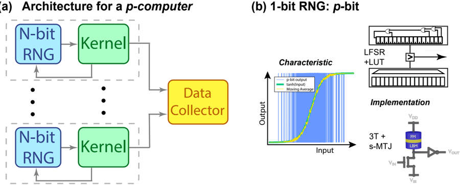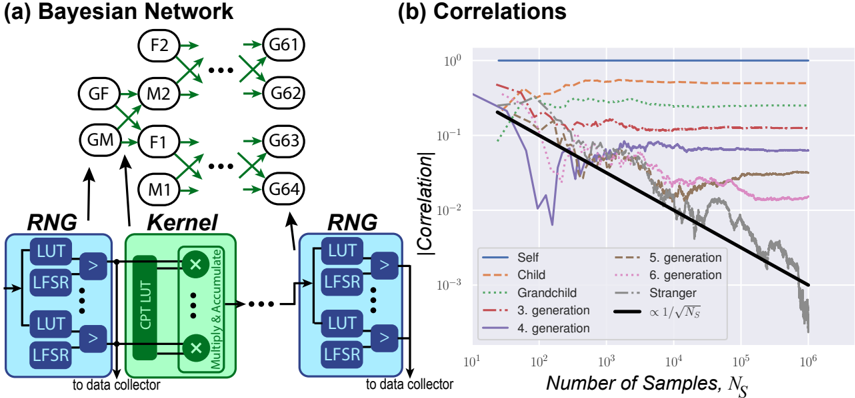A key element in a Monte Carlo algorithm is the RNG which requires thousands of transistors to implement with deterministic elements, thus encouraging the use of architectures that time share a few RNG's. Our work has shown the possibility of high quality true RNG's using just three transistors 3 , prompting us to explore a different architecture that makes use of large numbers of controlled-RNG's or p-bits . Fig. 1 (a) 4 shows a generic vision for a probabilistic or a p-computer having two primary components: an N-bit random number generator (RNG) that generates N-bit samples and a Kernel that performs deterministic operations on them. Note that each RNG-Kernel unit could include multiple RNGKernel sub-units (not shown) for problems that can benefit from it. These sub-units could be connected in series as in Bayesian networks (Fig. 2 (a) or in parallel as done in parallel tempering 5,6 or for problems that allow graph coloring 7 . The parallel RNG-Kernel units shown in Fig. 1 (a) are intended to perform easily parallelizable operations like ensemble sums using a data collector unit to combine all outputs into a single consolidated output. a) kaiser32@purdue.edu Ideally the Kernel and data collector are pipelined so that they can continually accept new random numbers from the RNG 4 , which is assumed to be fast and available in numerous numbers. The p-computer can then provide N p f c samples per second, N p being the number of parallel units 9 , and f c the clock frequency. We argue that even with N p = 1, this throughput is well in excess of what is achieved with standard implementations on either CPU (central processing unit) or GPU (graphics processing unit) for a broad range of applications and algorithms including but not limited to those targeted by modern digital annealers or Ising solvers 8,10-17 . Interestingly, a p-computer also provides a conceptual bridge to quantum computing, sharing many characteristics that we associate with the latter 18 . Indeed it can implement algorithms intended for quantum computers, though the effectiveness of quantum Monte Carlo depends strongly on the extent of the so-called sign problem specific to the algorithm and our ability to 'tame' it 19 . ## II. IMPLEMENTATION Of the three elements in Fig. 1, two are deterministic . The Kernel is problem-specific ranging from simple operations like addition or multiplication to more elaborate operations that could justify special purpose chiplets 20 . Matrix multiplication for example could be implemented using analog options like resistive crossbars 16,21-23 . The data collector typically involves addition and could be implemented with adder trees. The third element is probabilistic , namely the N-bit RNG which is a collection of N 1-bit RNG's or p -bits . The behavior of each p -bit can be described by 24 $$s _ { i } = \Theta [ \, \sigma ( I _ { i } - r ) \, ] \quad \, ( 1 )$$ where s i is the binary p-bit output, Θ is the step function, σ is the sigmoid function, I i is the input to the p-bit and r is a uniform random number between 0 and 1. Eq. (1) is illustrated in Fig. 1 (b). While the p-bit output is always binary, the p-bit input I i influences the mean of the output sequence. With I i = 0, the output FIG. 1. Probabilistic computer: (a) Overall architecture combining a probabilistic element (N-bit RNG) with deterministic elements (kernel and data collector). The N-bit RNG block is a collection of N 1-bit RNG's, or p-bits. (b) p-bit: Desired input-output characteristic along with two possible implementations, one with CMOS technology using linear feedback shift registers (LFSR's) and lookup tables (LUT's) 8 and the other using three transistors and a stochastic magnetic tunnel junction (s-MTJ) 3 . The first is used to obtain all the results presented here, while the second is a nascent technology with many unanswered questions. <details> <summary>Image 1 Details</summary>  ### Visual Description ## System Architecture and RNG Characteristics ### Overview The image presents two diagrams. Diagram (a) illustrates the architecture for a p-computer, showing interconnected N-bit Random Number Generators (RNGs), Kernels, and a Data Collector. Diagram (b) details a 1-bit RNG, including its characteristic curve and implementation details. ### Components/Axes #### Diagram (a): Architecture for a p-computer * **Title:** Architecture for a p-computer * **Components:** * N-bit RNG (light blue rounded rectangle) * Kernel (light green rounded rectangle) * Data Collector (yellow rounded rectangle) * **Flow:** N-bit RNG -> Kernel -> Data Collector. There is also a feedback loop from the Kernel back to the N-bit RNG. The entire structure is repeated multiple times, indicated by ellipsis. #### Diagram (b): 1-bit RNG: p-bit * **Title:** 1-bit RNG: p-bit * **Sub-diagram 1: Characteristic** * **Axes:** * X-axis: Input * Y-axis: Output * **Data Series (Legend, located at the top-center of the sub-diagram):** * p-bit output (light blue vertical lines) * tanh(Input) (light green line) * Moving Average (light yellow line) * **Sub-diagram 2: LFSR + LUT** * Shows a Linear Feedback Shift Register (LFSR) combined with a Look-Up Table (LUT). * **Sub-diagram 3: Implementation** * Shows a circuit diagram including: * VDD (supply voltage) * 3T + s-MTJ (3 Transistors + spin-Magnetic Tunnel Junction) * FM (Ferromagnetic layer) * LBM (Layer Below Magnetic layer) * VIN (input voltage) * VSS (ground voltage) * VOUT (output voltage) ### Detailed Analysis #### Diagram (a): Architecture for a p-computer The architecture consists of multiple parallel units. Each unit contains an N-bit RNG that feeds into a Kernel. The output of the Kernels is collected by a Data Collector. There is a feedback loop from the Kernel back to the N-bit RNG. #### Diagram (b): 1-bit RNG: p-bit * **Characteristic Curve:** The "p-bit output" is represented by a series of light blue vertical lines, showing a noisy output. The "tanh(Input)" is a light green sigmoid curve, representing a hyperbolic tangent function of the input. The "Moving Average" is a light yellow line that smooths out the p-bit output, closely following the tanh(Input) curve. * **LFSR + LUT:** The diagram shows a basic structure of an LFSR combined with a LUT, which is used to generate pseudo-random numbers. * **Implementation:** The circuit diagram shows a 3T + s-MTJ implementation, which includes a spin-MTJ device. ### Key Observations * **Diagram (a):** The architecture is parallel, suggesting that the p-computer utilizes multiple RNGs and Kernels to generate and process data. * **Diagram (b):** The characteristic curve shows that the p-bit output is noisy, but the moving average smooths it out to approximate a tanh function. The implementation uses a 3T + s-MTJ circuit. ### Interpretation The diagrams illustrate the architecture and implementation of a p-computer and its 1-bit RNG component. The parallel architecture in (a) suggests a design for high throughput or parallel processing. The characteristic curve in (b) shows the behavior of the 1-bit RNG, where the moving average of the noisy p-bit output approximates a tanh function, which is likely used for some form of probabilistic computation. The implementation details in (b) indicate the use of spintronic devices (s-MTJ) in the RNG design. </details> is distributed 50 -50 between 0 and 1 and this may be adequate for many algorithms. But in general a nonzero I i determined by the current sample is necessary to generate desired probability distributions from the N-bit RNG -block. One promising implementation of a p-bit is based on a stochastic magnetic tunnel junction (s-MTJ) as shown in Fig. 1 (b) whose resistance state fluctuates due to thermal noise. It is placed in series with a transistor, and the drain voltage is thresholded by an inverter 3 to obtain a random binary output bit whose average value can be tuned through the gate voltage V IN . It has been shown both theoretically 25,26 and experimentally 27,28 that sMTJ -based p-bits can be designed to generate new random numbers in times ∼ nanoseconds . The same circuit could also be used with other fluctuating resistors 29 , but one advantage of s-MTJ's is that they can be built by modifying magnetoresistive random access memory (MRAM) technology that has already reached gigabit levels of integration 30 . Note, however, that the examples presented here all use p-bits implemented with deterministic CMOS elements or pseudo-RNG's using linear feedback shift registers (LFSR's) combined with lookup tables (LUT's) and thresholding elements 8 as shown in Fig. 1 (b). Such random numbers are not truly random, but have a period that is longer than the time range of interest. The longer the period, the more registers are needed to implement it. Typically a p-bit requires ∼ 1000 transistors 30 , the actual number depending on the quality of the pseudo RNG that is desired. Thirty-two stage LFSR's require ∼ 1200 transistors, while a Xoshiro128+ 31 would require around four times as many. Physics-based approaches, like s-MTJ's , naturally generate true random numbers with infinite repetition period and ideally require only 3 transistors and 1 MTJ. A simple performance metric for p-computers is the ideal sampling rate N p f c mentioned above. The results presented here were all obtained with an fieldprogrammable gate array (FPGA) running on a 125 MHz clock, for which 1 /f c = 8 ns, which could be significantly shorter (even ∼ 0 . 1 ns 25 ) if implemented with s-MTJ's . Furthermore, s-MTJ's are compact and energy-efficient, allowing up to a factor of 100 larger N p for a given area and power budget. With an increase of f c and N p , a performance improvement by 2-3 orders of magnitude over the numbers presented here may be possible with s-MTJ's or other physics-based hardware. We should point out that such compact p-bit implementations are still in their infancy 30 and many questions remain. First is the inevitable variation in RNG characteristics that can be expected. Initial studies suggest that it may be possible to train the Kernel to compensate for at least some of these variations 32,33 . Second is the quality of randomness, as measured by statistical quality tests which may require additional circuitry as discussed for example in Ref. 27 . Certain applications like simple integration (Section III A) may not need high quality random numbers, while others like Bayesian correlations (Section III B) or Metropolis-Hastings methods that require a proposal distribution (Section III C) may have more stringent requirements. Third is the possible difficulty associated with reading sub-nanosecond fluctuations in the output and communicating them faithfully. Finally, we note that the input to a p-bit is an analog quantity requiring Digital-to-Analog Converters (DAC's) FIG. 2. Bayesian network for genetic relatedness mapped to a p-computer (a) with each node represented by one p-bit. With increasing N S , the correlations (b) between different nodes is obtained more accurately. <details> <summary>Image 2 Details</summary>  ### Visual Description ## Bayesian Network and Correlations ### Overview The image presents two diagrams: (a) a Bayesian Network illustrating relationships between family members, and (b) a plot showing the correlation between individuals as a function of the number of samples. ### Components/Axes #### (a) Bayesian Network * **Title:** (a) Bayesian Network * **Nodes:** Represented by circles, labeled as F2, GF, GM, M2, F1, M1, G61, G62, G63, G64. These likely represent family members (e.g., GF = Grandfather, GM = Grandmother, F = Father, M = Mother, G = Generation). * **Edges:** Green arrows indicating probabilistic dependencies between nodes. * **RNG (Random Number Generator) Blocks:** Two blue blocks labeled "RNG" containing "LUT" (Look-Up Table) and "LFSR" (Linear Feedback Shift Register) components. Arrows point from these blocks to the Bayesian Network. Text "to data collector" is present below each RNG block. * **Kernel Block:** A green block labeled "Kernel" containing "CPT LUT" (Conditional Probability Table Look-Up Table) and "Multiply & Accumulate" components. An arrow points from this block to the Bayesian Network. #### (b) Correlations * **Title:** (b) Correlations * **Y-axis:** |Correlation|, logarithmic scale from 10^-3 to 10^0. * **X-axis:** Number of Samples, N_s, logarithmic scale from 10^1 to 10^6. * **Legend:** Located in the bottom-center of the plot. * Self (solid blue line) * Child (dashed red line) * Grandchild (dotted green line) * 3. generation (dash-dot red line) * 4. generation (solid purple line) * 5. generation (dashed gray line) * 6. generation (dotted pink line) * Stranger (dash-dot gray line) * ∝ 1/√N_s (solid black line) ### Detailed Analysis #### (a) Bayesian Network The Bayesian network shows a hierarchical structure. The RNG and Kernel blocks feed into the network, suggesting they provide the initial data or parameters for the probabilistic relationships. The arrows indicate the flow of influence between family members. * RNG blocks contain "LUT" and "LFSR" components. * Kernel block contains "CPT LUT" and "Multiply & Accumulate" components. #### (b) Correlations The plot shows how the correlation between individuals changes as the number of samples increases. * **Self (solid blue line):** Remains constant at approximately 1. * **Child (dashed red line):** Starts around 0.3 and remains relatively constant. * **Grandchild (dotted green line):** Starts around 0.2 and remains relatively constant. * **3. generation (dash-dot red line):** Starts around 0.1 and remains relatively constant. * **4. generation (solid purple line):** Starts around 0.05, decreases sharply until ~10^3 samples, then fluctuates around 0.01. * **5. generation (dashed gray line):** Starts around 0.05, decreases sharply until ~10^3 samples, then fluctuates around 0.01. * **6. generation (dotted pink line):** Starts around 0.05, decreases sharply until ~10^3 samples, then fluctuates around 0.01. * **Stranger (dash-dot gray line):** Starts around 0.05, decreases sharply until ~10^3 samples, then fluctuates around 0.01. * **∝ 1/√N_s (solid black line):** A reference line showing a decay proportional to the inverse square root of the number of samples. This line serves as a benchmark for how correlation should decrease with increasing sample size if the correlation is due to random chance. ### Key Observations * The correlation for "Self" remains constant at 1, as expected. * The correlation decreases as the generational distance increases (Child > Grandchild > 3rd Generation). * For generations beyond the 3rd, the correlation decreases sharply initially and then fluctuates around a low value. * The correlation decay for distant generations (4th, 5th, 6th, Stranger) roughly follows the ∝ 1/√N_s trend after an initial drop. ### Interpretation The Bayesian Network illustrates the relationships between family members, while the correlation plot quantifies the strength of these relationships as a function of the number of samples. The plot demonstrates that correlation decreases with generational distance, indicating that closer relatives have stronger correlations. The decay of correlation for distant relatives follows the ∝ 1/√N_s trend, suggesting that the observed correlation is largely due to random chance and decreases as more data is collected. The RNG and Kernel blocks in the Bayesian Network likely represent the mechanisms by which the data is generated and processed to calculate these correlations. </details> unless the kernel itself is implemented with analog components. ## III. APPLICATIONS ## A. Simple integration Avariety of problems such as high dimensional integration can be viewed as the evaluation of a sum over a very large number N of terms. The basic idea of the Monte Carlo method is to estimate the desired sum from a limited number N s of samples drawn from configurations α generated with probability q α : $$M = \sum _ { \alpha = 1 } ^ { N } m _ { \alpha } \approx \frac { 1 } { N _ { S } } \sum _ { \alpha = 1 } ^ { N _ { S } } \frac { m _ { \alpha } } { q _ { \alpha } } \quad ( 2 ) \quad H o n$$ The distribution { q } can be uniform or could be cleverly chosen to minimize the standard deviation of the estimate 34 . In any case the standard deviation goes down as 1 / √ N s and all such applications could benefit from a p-computer to accelerate the collection of samples. ## B. Bayesian Network A little more complicated application of a p-computer is to problems where random numbers are generated not according to a fixed distribution, but by a distribution determined by the outputs from a previous set of RNG ′ s . Consider for example the question of genetic relatedness in a family tree 35,36 with each layer representing one generation. Each generation in the network in Fig. 2 (a) with N nodes can be mapped to a N-bit RNG -block feeding into a Kernel which stores the conditional probability table (CPT) relating it to the next generation. The correlation between different nodes in the network can be directly measured and an average over the samples computed to yield the correct genetic correlation as shown in Fig. 2 (b). Nodes separated by p generations have a correlation of 1 / 2 p . The measured absolute correlation between strangers goes down to zero as 1 / √ N s . This is characteristic of Monte Carlo algorithms, namely, to obtain results with accuracy ε we need N s = 1 /ε 2 samples. The p-computer allows us to collect samples at the rate of N p f c = 125 MSamples per second if N p = 1 and f c = 125 MHz. This is about two orders of magnitude faster than what we get running the same algorithm on a Intel Xeon CPU. How does it compare to deterministic algorithms run on CPU ? As Feynman noted in his seminal paper 1 , deterministic algorithms for problems of this type are very inefficient compared to probabilistic ones because of the need to integrate over all the unobserved nodes { x B } in order to calculate a property related to nodes { x A } $$P _ { A } ( x _ { A } ) = \int d x _ { B } P ( x _ { A } , x _ { B } ) \quad \quad ( 3 )$$ By contrast, a p-computer can ignore all the irrelevant nodes { x b } and simply look at the relevant nodes { x A } . We used the example of genetic correlations because it is easy to relate to. But it is representative of a wide class of everyday problems involving nodes with oneway causal relationships extending from 'parent' nodes to 'child' nodes 37-39 , all of which could benefit from a p-computer . 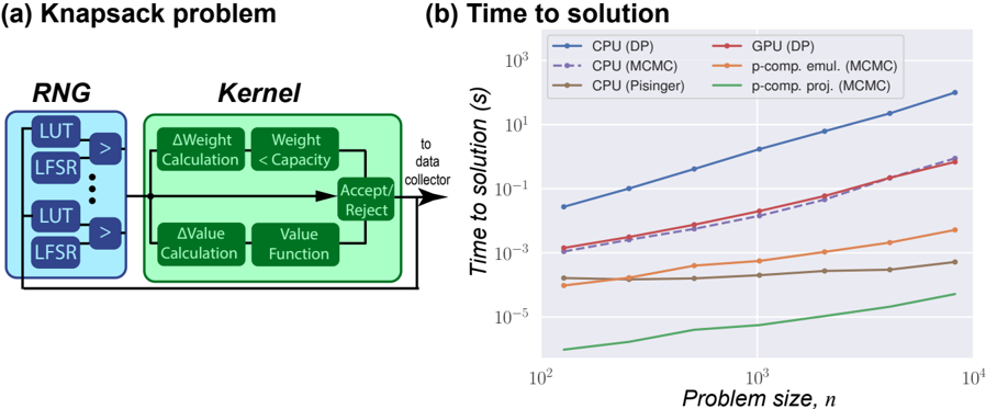FIG. 3. Example of MCMC - Knapsack problem: (a) Mapping to the general p-computer framework. (b) Performance of the p-computer compared to CPU implementation of the same probabilistic algorithm and along with two well-known deterministic approaches. A deterministic algorithm like Pisinger's 40 which is optimized specifically for the Knapsack problem can outperform MCMC. But for a given MCMC algorithm, the p-computer provides orders of magnitude improvement over the standard CPU implementation. <details> <summary>Image 3 Details</summary>  ### Visual Description ## Diagram and Chart: Knapsack Problem and Time to Solution ### Overview The image presents two sub-figures: (a) a diagram illustrating the components of a Knapsack problem solver, and (b) a chart comparing the time to solution for different algorithms (CPU and GPU implementations) as a function of problem size. ### Components/Axes #### (a) Knapsack Problem Diagram * **Title:** Knapsack problem * **Components:** * **RNG (Random Number Generator):** Contains multiple LUT (Look-Up Table) and LFSR (Linear Feedback Shift Register) pairs. Arrows indicate data flow from each LUT/LFSR pair to a comparator (>). * **Kernel:** Contains two parallel processes: * **Top Branch:** ΔWeight Calculation followed by Weight < Capacity comparison. * **Bottom Branch:** ΔValue Calculation followed by Value Function. * **Accept/Reject:** A decision block that receives input from both branches of the Kernel. * **Data Flow:** The output of the Accept/Reject block is fed back into the Kernel, creating a loop. The output also goes "to data collector". #### (b) Time to Solution Chart * **Title:** Time to solution * **X-axis:** Problem size, *n*. Logarithmic scale from approximately 10² to 10⁴. Axis markers at 10², 10³, and 10⁴. * **Y-axis:** Time to solution (s). Logarithmic scale from approximately 10^-5 to 10³. Axis markers at 10^-5, 10^-3, 10^-1, 10¹, and 10³. * **Legend (Top-Left):** * Blue solid line: CPU (DP) * Purple dashed line: CPU (MCMC) * Brown solid line: CPU (Pisinger) * Red solid line: GPU (DP) * Orange solid line: p-comp. emul. (MCMC) * Green solid line: p-comp. proj. (MCMC) ### Detailed Analysis #### (a) Knapsack Problem Diagram The diagram illustrates the core components of a knapsack problem solver. The RNG generates random numbers used by the Kernel to evaluate potential solutions. The Kernel calculates changes in weight and value, and the Accept/Reject block determines whether to accept the new solution or reject it. The feedback loop allows the algorithm to iteratively refine the solution. #### (b) Time to Solution Chart * **CPU (DP) - Blue Solid Line:** The time to solution increases rapidly with problem size. * At n = 100, time ≈ 0.03 s * At n = 1000, time ≈ 1 s * At n = 10000, time ≈ 100 s * **CPU (MCMC) - Purple Dashed Line:** The time to solution increases rapidly with problem size, but is lower than CPU (DP). * At n = 100, time ≈ 0.001 s * At n = 1000, time ≈ 0.03 s * At n = 10000, time ≈ 3 s * **CPU (Pisinger) - Brown Solid Line:** The time to solution remains relatively constant with problem size. * At n = 100, time ≈ 0.00003 s * At n = 1000, time ≈ 0.00005 s * At n = 10000, time ≈ 0.0001 s * **GPU (DP) - Red Solid Line:** The time to solution increases rapidly with problem size, and is lower than CPU (DP). * At n = 100, time ≈ 0.001 s * At n = 1000, time ≈ 0.03 s * At n = 10000, time ≈ 3 s * **p-comp. emul. (MCMC) - Orange Solid Line:** The time to solution remains relatively constant with problem size. * At n = 100, time ≈ 0.00005 s * At n = 1000, time ≈ 0.0002 s * At n = 10000, time ≈ 0.001 s * **p-comp. proj. (MCMC) - Green Solid Line:** The time to solution remains relatively constant with problem size. * At n = 100, time ≈ 0.00001 s * At n = 1000, time ≈ 0.00002 s * At n = 10000, time ≈ 0.00005 s ### Key Observations * The CPU (DP) algorithm has the highest time to solution, increasing dramatically with problem size. * The CPU (MCMC) and GPU (DP) algorithms have similar performance, with the GPU implementation being slightly faster. * The CPU (Pisinger), p-comp. emul. (MCMC), and p-comp. proj. (MCMC) algorithms have significantly lower time to solution, and their performance is relatively independent of problem size. ### Interpretation The chart demonstrates the performance differences between various algorithms for solving the Knapsack problem. Dynamic Programming (DP) implementations (CPU and GPU) exhibit a steep increase in time to solution as the problem size grows, indicating a higher computational complexity. Markov Chain Monte Carlo (MCMC) methods, especially when parallelized (p-comp. emul. and p-comp. proj.), show a much flatter curve, suggesting better scalability for larger problem instances. The Pisinger algorithm on the CPU also shows excellent performance and scalability. The data suggests that for larger Knapsack problems, MCMC-based or Pisinger algorithms are significantly more efficient than DP-based approaches. The GPU implementation of DP offers a modest improvement over the CPU version, but the algorithmic choice has a much greater impact on performance. </details> ## C. Knapsack Problem Let us now look at a problem which requires random numbers to be generated with a probability determined by the outcome from the last sample generated by the same RNG. Every RNG then requires feedback from the very Kernel that processes its output. This belongs to the broad class of problems that are labeled as Markov Chain Monte Carlo (MCMC) . For an excellent summary and evaluation of MCMC sampling techniques we refer the reader to Ref. 41 . The knapsack is a textbook optimization problem described in terms of a set of items, m = 1 , · · N , the m th , each containing a value v m and weighing w m . The problem is to figure out which items to take ( s m = 1) and which to leave behind ( s m = 0) such that the total value V = ∑ m v m s m is a maximum, while keeping the total weight W = ∑ m w m s m below a capacity C . We could straightforwardly map it to the p -computer architecture (Fig. 1), using the RNG to propose solutions { s } at random, and the Kernel to evaluate V, W and decide to accept or reject. But this approach would take us toward the solution far too slowly. It is better to propose solutions intelligently looking at the previous accepted proposal, and making only a small change to it. For our examples we proposed a change of only two items each time. This intelligent proposal, however, requires feedback from the kernel which can take multiple clock cycles. One could wait between proposals, but the solution is faster if instead we continue to make proposals every clock cycle in the spirit of what is referred to as multiple-try Metropolis 42 . The results are shown in Fig. 3 4 and compared with CPU (Intel Xeon @ 2.3GHz) and GPU (Tesla T4 @ 1.59GHz) implementations, using the probabilistic algorithm. Also shown are two efficient deterministic algorithms, one based on dynamic programming (DP), and one due to Pisinger et al. 40,43 . Note that the probabilistic algorithm (MCMC) gives solutions that are within 1% of the correct solution, while the deterministic algorithms give the correct solution. For the Knapsack problem getting a solution that is 99% accurate should be sufficient for most real world applications. The p-computer provides orders of magnitude improvement over CPU implementation of the same MCMC algorithm. It is outperformed by the algorithm developed by Pisinger et al. 40,43 , which is specifically optimized for the Knapsack problem. However, we note that the pcomputer projection in Fig. 3 (b) is based on utilizing better hardware like s-MTJ's but there is also significant room for improvement of the p-computer by optimizing the Metropolis algorithm used here and/or by adding parallel tempering 5,6 . ## D. Ising model Another widely used model for optimization within MCMC is based on the concept of Boltzmann machines (BM) defined by an energy function E from which one can calculate the synaptic function I i $$I _ { i } = \beta ( E ( s _ { i } = 0 ) - E ( s _ { i } = 1 ) ) , \quad \ \ ( 4 )$$ that can be used to guide the sample generation from each RNG 'i' in sequence 44 according to Eq. (1). 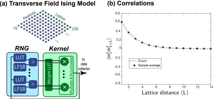Alternatively the sample generation from each RNG FIG. 4. Example of Quantum Monte Carlo (QMC) - Transverse Field Ising model: (a) Mapping to the general p-computer framework. (b) Solving the transverse Ising model for quantum annealing. Subfigure (b) is adapted from B. Sutton, R. Faria, L. A. Ghantasala, R. Jaiswal, K. Y. Camsari and S. Datta, IEEE Access, vol. 8, pp. 157238-157252, 2020 licensed under a Creative Commons Attribution (CC BY) license 8 . <details> <summary>Image 4 Details</summary>  ### Visual Description ## Chart/Diagram: Transverse Field Ising Model and Correlations ### Overview The image presents two diagrams. The first (a) illustrates a Transverse Field Ising Model with a lattice structure and a computational flow diagram involving a Random Number Generator (RNG) and a Kernel. The second (b) is a plot showing the correlation as a function of lattice distance, comparing an "Exact" theoretical curve with "Sample average" data. ### Components/Axes **Part (a): Transverse Field Ising Model** * **Title:** Transverse Field Ising Model * **Lattice:** A 2D lattice structure is depicted with blue dots, labeled as "Lattice" on the right edge with green dots. The number of lattice points is indicated as 10 on the left edge and 250 on the right edge. * **Replicas:** The lattice is also labeled as "Replicas" on the top edge with blue dots. * **RNG (Random Number Generator):** A blue box labeled "RNG" contains two pairs of "LUT" (Look-Up Table) and "LFSR" (Linear Feedback Shift Register) components. Each pair is connected by a ">" symbol, suggesting a flow or comparison. * **Kernel:** A green box labeled "Kernel" contains "Weight LUT" and "Multiply & Accumulate" components. * **Flow:** The output from the RNG flows into the Kernel. The output of the Kernel is directed "to data collector" via an arrow. **Part (b): Correlations** * **Title:** Correlations * **X-axis:** Lattice distance (L), ranging from 2 to 14 in increments of 2. * **Y-axis:** `<m₁ᶻm₁₊Lᶻ>`, ranging from -0.8 to 0.8 in increments of 0.2. * **Data Series 1:** "Exact" - Represented by a dashed black line. * **Data Series 2:** "Sample average" - Represented by blue dots. ### Detailed Analysis **Part (a): Transverse Field Ising Model** * The lattice structure is a grid, with the number of points increasing from left to right. * The RNG and Kernel represent a computational process, likely used to simulate the Ising Model. * The flow diagram indicates that random numbers generated by the RNG are used in the Kernel to perform calculations, and the results are then collected. **Part (b): Correlations** * **Exact (dashed black line):** Starts at approximately 0.6 at L=2 and decreases rapidly, approaching 0 as L increases. * **Sample average (blue dots):** Starts at approximately 0.58 at L=2 and decreases, closely following the trend of the "Exact" line. The values appear to level off around 0.08 for L > 10. Here are the approximate data points for the "Sample average" series: * L=2: 0.58 * L=3: 0.38 * L=4: 0.23 * L=5: 0.16 * L=6: 0.12 * L=7: 0.10 * L=8: 0.09 * L=9: 0.08 * L=10: 0.08 * L=11: 0.07 * L=12: 0.07 * L=13: 0.06 * L=14: 0.06 ### Key Observations * The correlation decreases as the lattice distance increases. * The "Sample average" data closely matches the "Exact" theoretical curve, suggesting the simulation is accurate. * The correlation approaches zero at larger lattice distances, indicating that spins become less correlated as the distance between them increases. ### Interpretation The image illustrates the simulation and analysis of a Transverse Field Ising Model. The model is simulated using a computational process involving random number generation and a kernel. The correlation between spins at different lattice distances is then calculated and compared to a theoretical prediction. The close agreement between the simulation results and the theoretical curve validates the simulation method and provides insights into the behavior of the Ising Model. The decay of correlation with distance is a key characteristic of this model. </details> can be fixed and the synaptic function used to decide whether to accept or reject it within a MetropolisHastings framework 45 . Either way, samples will be generated with probabilities P α ∼ exp ( -βE α ). We can solve optimization problems by identifying E with the negative of the cost function that we are seeking to minimize. Using a large β we can ensure that the probability is nearly 1 for the configuration with the minimum value of E. In principle, the energy function is arbitrary, but much of the work is based on quadratic energy functions defined by a connection matrix W ij and a bias vector h i (see for example 8,10-17 ): $$E = - \sum _ { i j } W _ { i j } s _ { i } s _ { j } - \sum _ { i } h _ { i } s _ { i } , \quad ( 5 ) \quad o r a$$ For this quadratic energy function, Eq. (4) gives I i = β ( ∑ j W ij s j + h i ) , so that the Kernel has to perform a multiply and accumulate operation as shown in Fig. 4 (a). We refer the reader to Sutton et al. 8 for an example of the max-cut optimization problem on a two-dimensional 90 × 90 array implemented with a pcomputer . Eq. (4), however, is more generally applicable even if the energy expression is more complicated, or given by a table. The Kernel can be modified accordingly. For an example of a energy function with fourth order terms implemented on an eight bit p-computer , we refer the reader to Borders et al. 30 . A wide variety of problems can be mapped onto the BM with an appropriate choice of the energy function. For example, we could generate samples from a desired probability distribution P , by choosing βE = -nP . Another example is the implementation of logic gates by defining E to be zero for all { s } that belong to the truth table, and have some positive value for those that do not 24 . Unlike standard digital logic, such a BM-based implementation would provide invertible logic that not only provides the output for a given input, but also generates all possible inputs corresponding to a specified output 24,46,47 . ## E. Quantum Monte Carlo Finally let us briefly describe the feasibility of using p-computers to emulate quantum or q-computers. A qcomputer is based on qubits that are neither 0 or 1, but are described by a complex wavefunction whose squared magnitude gives the probability of measuring either a 0 or a 1. The state of an n -qubit computer is described by a wavefunction { ψ } with 2 n complex components, one for each possible configuration of the n qubits. In gate-based quantum computing (GQC) a set of qubits is placed in a known state at time t , operated on with d quantum gates to manipulate the wavefunction through unitary transformations [ U ( i ) ] $$\begin{array} { r l r l } & { a p ^ { - } } & \\ & { \left \{ \psi ( t + d ) \right \} = [ U ^ { ( d ) } ] \cdots \cdots [ U ^ { ( 1 ) } ] \{ \psi ( t ) \} } & & { ( G Q C ) \ ( 6 ) } \\ \end{array}$$ and measurements are made to obtain results with probabilities given by the squared magnitudes of the final wavefunctions. From the rules of matrix multiplication, the final wavefunction can be written as a sum over a very large number of terms: $$\psi _ { m } ( t + d ) = \sum _ { i , \cdot \cdot j , k } U _ { m , i } ^ { ( d ) } \cdots \cdots U _ { j , k } ^ { ( 1 ) } \, \psi _ { k } ( t ) \quad ( 7 )$$ Conceptually we could represent a system of n qubits and d gates with a system of ( n × d ) p-bits with 2 nd states which label the 2 nd terms in the summation in Eq.(7) 48 . Each of these terms is often referred to as a Feynman path and what we want is the sum of the amplitudes of all such paths: $$\psi _ { m } ( t + d ) = \sum _ { \alpha = 1 } ^ { 2 ^ { n d } } A _ { m } ^ { ( \alpha ) }$$ The essential idea of quantum Monte Carlo is to estimate this enormous sum from a few suitably chosen samples, not unlike the simple Monte Carlo stated earlier in Eq. (2). What makes it more difficult, however, is the socalled sign problem 19 which can be understood intuitively as follows. If all the quantities A ( α ) m are positive then it is relatively easy to estimate the sum from a few samples. But if some are positive while some are negative with lots of cancellations, then many more samples will be required. The same is true if the quantities are complex quantities that cancel each other. The matrices U that appear in GQC are unitary with complex elements which often leads to significant cancellation of Feynman paths, except in special cases when there may be complete constructive interference. In general this could make it necessary to use large numbers of samples for accurate estimation. A noiseless quantum computer would not have this problem, since qubits intuitively perform the entire sum exactly and yield samples according to the squared magnitude of the resulting wavefunction. However, real world quantum computers have noise and p-computers could be competitive for many problems. Adiabatic quantum computing (AQC) operates on very different physical principles but its mathematical description can also be viewed as summing the Feynman paths representing the multiplication of r matrices: $$[ e ^ { - \beta H / r } ] \cdots \, \cdot \cdot [ e ^ { - \beta H / r } ] \quad ( A Q C ) \quad ( 9 )$$ This is based on the Suzuki-Trotter method described in Camsari et al. 49 , where the number of replicas, r , is chosen large enough to ensure that if H = H 1 + H 2 , one can approximately write e -βH/r ≈ e -βH 1 /r e -βH 2 /r . The matrices e -βH/r in AQC are Hermitian, and their elements can be all positive 50 . A special class of Hamiltonians H having this property is called stoquastic and there is no sign problem since the amplitudes A ( α ) m in the Feynman sum in Eq. (8) all have the same sign. An example of such a stoquastic Hamiltonian is the transverse field Ising model (TFIM) commonly used for quantum annealing where a transverse field which is quantum in nature is introduced and slowly reduced to zero to recover the original classical problem. Fig. 4 adapted from Sutton et al. 8 , shows a n = 250 qubit problem mapped to a 2-D lattice of 250 × 10 = 2500 p-bits using r = 10 replicas to calculated average correlations between the z-directed spins on lattice sites separated by L . Very accurate results are obtained using N s = 10 5 samples. However,these samples were suitably spaced to ensure their independence, which is an important concern in problems involving feedback. Finally we note that quantum Monte Carlo methods, both GQC and AQC, involve selective summing of Feynman paths to evaluate matrix products. As such we might expect conceptual overlap with the very active field of randomized algorithms for linear algebra 51,52 , though the two fields seem very distinct at this time. ## IV. CONCLUDING REMARKS In summary, we have presented a generic architecture for a p-computer based on p-bits which take on values 0 and 1 with controlled probabilities, and can be implemented with specialized compact energy-efficient hardware. We emulate systems with thousands of p-bits to show that they can significantly accelerate the implementation of randomized algorithms that are widely used for many applications 53 . A few prototypical examples are presented such as Bayesian networks, optimization, Ising models and quantum Monte Carlo. ## ACKNOWLEDGMENTS The authors are grateful to Behtash Behin-Aein for helpful discussions and advice. We also thank Kerem Camsari and Shuvro Chowdhury for their feedback on the manuscript. The contents are based on the work done over the last 5-10 years in our group, some of which has been cited here, and it is a pleasure to acknowledge all who have contributed to our understanding. This work was supported in part by ASCENT, one of six centers in JUMP, a Semiconductor Research Corporation (SRC) program sponsored by DARPA. ## DATA AVAILABILITY The data that support the findings of this study are available from the corresponding author upon reasonable request. ## AUTHOR DECLARATIONS ## Conflict of interests One of the authors (SD) has a financial interest in Ludwig Computing. - 1 R. P. Feynman, 'Simulating physics with computers,' Int. J. Theor. Phys 21 (1982). - 2 B. A. Cipra, 'The Best of the 20th Century: Editors Name Top 10 Algorithms,' SIAM News 33 , 1-2 (2000). - 3 K. Y. Camsari, S. Salahuddin, and S. Datta, 'Implementing pbits with Embedded MTJ,' IEEE Electron Device Letters 38 , 1767-1770 (2017). - 4 J. Kaiser, R. Jaiswal, B. Behin-Aein, and S. Datta, 'Benchmarking a Probabilistic Coprocessor,' arXiv:2109.14801 [cond-mat] (2021), arXiv:2109.14801 [cond-mat]. - 5 R. Swendsen and J.-S. Wang, 'Replica Monte Carlo Simulation of Spin-Glasses,' Physical review letters 57 , 2607-2609 (1986). - 6 D. J. Earl and M. W. Deem, 'Parallel tempering: Theory, applications, and new perspectives,' Physical Chemistry Chemical Physics 7 , 3910-3916 (2005). - 7 G. G. Ko, Y. Chai, R. A. Rutenbar, D. Brooks, and G.-Y. Wei, 'Accelerating Bayesian Inference on Structured Graphs Using Parallel Gibbs Sampling,' in 2019 29th International Conference on Field Programmable Logic and Applications (FPL) (IEEE, Barcelona, Spain, 2019) pp. 159-165. - 8 B. Sutton, R. Faria, L. A. Ghantasala, R. Jaiswal, K. Y. Camsari, and S. Datta, 'Autonomous Probabilistic Coprocessing with Petaflips per Second,' IEEE Access , 1-1 (2020). - 9 Here, we assume that every RNG-Kernel unit gives one sample per clock cycle. There could be cases where multiple samples could be extracted from one unit per clock cycle. - 10 H. Goto, K. Tatsumura, and A. R. Dixon, 'Combinatorial optimization by simulating adiabatic bifurcations in nonlinear Hamiltonian systems,' Science Advances 5 , eaav2372 (2019). - 11 M. Aramon, G. Rosenberg, E. Valiante, T. Miyazawa, H. Tamura, and H. G. Katzgraber, 'Physics-Inspired Optimization for Quadratic Unconstrained Problems Using a Digital Annealer,' Frontiers in Physics 7 (2019), 10.3389/fphy.2019.00048. - 12 K. Yamamoto, K. Ando, N. Mertig, T. Takemoto, M. Yamaoka, H. Teramoto, A. Sakai, S. Takamaeda-Yamazaki, and M. Motomura, '7.3 STATICA: A 512-Spin 0.25M-Weight Full-Digital Annealing Processor with a Near-Memory All-Spin-Updates-atOnce Architecture for Combinatorial Optimization with Complete Spin-Spin Interactions,' in 2020 IEEE International SolidState Circuits Conference - (ISSCC) (IEEE, San Francisco, CA, USA, 2020) pp. 138-140. - 13 M. Yamaoka, C. Yoshimura, M. Hayashi, T. Okuyama, H. Aoki, and H. Mizuno, '24.3 20k-spin Ising chip for combinational optimization problem with CMOS annealing,' in 2015 IEEE International Solid-State Circuits Conference - (ISSCC) Digest of Technical Papers (2015) pp. 1-3. - 14 I. Ahmed, P.-W. Chiu, and C. H. Kim, 'A Probabilistic SelfAnnealing Compute Fabric Based on 560 Hexagonally Coupled Ring Oscillators for Solving Combinatorial Optimization Problems,' in 2020 IEEE Symposium on VLSI Circuits (IEEE, Honolulu, HI, USA, 2020) pp. 1-2. - 15 S. Patel, L. Chen, P. Canoza, and S. Salahuddin, 'Ising Model Optimization Problems on a FPGA Accelerated Restricted Boltzmann Machine,' arXiv:2008.04436 [physics] (2020), arXiv:2008.04436 [physics]. - 16 F. Cai, S. Kumar, T. Van Vaerenbergh, X. Sheng, R. Liu, C. Li, Z. Liu, M. Foltin, S. Yu, Q. Xia, J. J. Yang, R. Beausoleil, W. D. Lu, and J. P. Strachan, 'Power-efficient combinatorial optimization using intrinsic noise in memristor Hopfield neural networks,' Nature Electronics 3 , 409-418 (2020). - 17 S. Dutta, A. Khanna, A. S. Assoa, H. Paik, D. G. Schlom, Z. Toroczkai, A. Raychowdhury, and S. Datta, 'An Ising Hamiltonian solver based on coupled stochastic phase-transition nanooscillators,' Nature Electronics 4 , 502-512 (2021). - 18 K. Camsari and S. Datta, 'Dialogue Concerning the Two Chief Computing Systems: Imagine yourself on a flight talking to an engineer about a scheme that straddles classical and quantum,' IEEE Spectrum 58 , 30-35 (2021). - 19 M. Troyer and U.-J. Wiese, 'Computational Complexity and Fundamental Limitations to Fermionic Quantum Monte Carlo Simulations,' Physical Review Letters 94 , 170201 (2005). - 20 T. Li, J. Hou, J. Yan, R. Liu, H. Yang, and Z. Sun, 'Chiplet Heterogeneous Integration Technology-Status and Challenges,' Electronics 9 , 670 (2020). - 21 C. Liu, B. Yan, C. Yang, L. Song, Z. Li, B. Liu, Y. Chen, H. Li, Q. Wu, and H. Jiang, 'A spiking neuromorphic design with resistive crossbar,' in 2015 52nd ACM/EDAC/IEEE Design Automation Conference (DAC) (IEEE, 2015) pp. 1-6. - 22 B. Li, Y. Shan, M. Hu, Y. Wang, Y. Chen, and H. Yang, 'Memristor-based approximated computation,' in International Symposium on Low Power Electronics and Design (ISLPED) (IEEE, 2013) pp. 242-247. 23 M. Demler, 'MYTHIC MULTIPLIES IN A FLASH,' , 3 (2018). - 24 K. Y. Camsari, R. Faria, B. M. Sutton, and S. Datta, 'Stochastic p -Bits for Invertible Logic,' Physical Review X 7 (2017), 10.1103/PhysRevX.7.031014. - 25 J. Kaiser, A. Rustagi, K. Y. Camsari, J. Z. Sun, S. Datta, and P. Upadhyaya, 'Subnanosecond Fluctuations in Low-Barrier Nanomagnets,' Physical Review Applied 12 , 054056 (2019). - 26 S. Kanai, K. Hayakawa, H. Ohno, and S. Fukami, 'Theory of relaxation time of stochastic nanomagnets,' Physical Review B 103 , 094423 (2021). - 27 C. Safranski, J. Kaiser, P. Trouilloud, P. Hashemi, G. Hu, and J. Z. Sun, 'Demonstration of Nanosecond Operation in Stochastic Magnetic Tunnel Junctions,' Nano Letters 21 , 2040-2045 (2021). - 28 K. Hayakawa, S. Kanai, T. Funatsu, J. Igarashi, B. Jinnai, W. A. Borders, H. Ohno, and S. Fukami, 'Nanosecond Random Telegraph Noise in In-Plane Magnetic Tunnel Junctions,' Physical Review Letters 126 , 117202 (2021). - 29 O. Hassan, S. Datta, and K. Y. Camsari, 'Quantitative Evaluation of Hardware Binary Stochastic Neurons,' Physical Review Applied 15 , 064046 (2021). - 30 W. A. Borders, A. Z. Pervaiz, S. Fukami, K. Y. Camsari, H. Ohno, and S. Datta, 'Integer factorization using stochastic magnetic tunnel junctions,' Nature 573 , 390-393 (2019). - 31 S. Vigna, 'Further scramblings of Marsaglia's xorshift generators,' Journal of Computational and Applied Mathematics 315 , 175-181 (2017). - 32 J. Kaiser, R. Faria, K. Y. Camsari, and S. Datta, 'Probabilistic Circuits for Autonomous Learning: A simulation study,' Frontiers in Computational Neuroscience 14 (2020), 10.3389/fncom.2020.00014. - 33 J. Kaiser, W. A. Borders, K. Y. Camsari, S. Fukami, H. Ohno, and S. Datta, 'Hardware-aware in-situ Boltzmann machine learning using stochastic magnetic tunnel junctions,' arXiv:2102.05137 [cond-mat] (2021), arXiv:2102.05137 [condmat]. - 34 C. M. Bishop, Pattern Recognition and Machine Learning: All 'Just the Facts 101' Material (Springer (India) Private Limited, 2013). - 35 R. Faria, J. Kaiser, K. Y. Camsari, and S. Datta, 'Hardware Design for Autonomous Bayesian Networks,' Frontiers in Computational Neuroscience 15 (2021), 10.3389/fncom.2021.584797. - 36 R. Faria, K. Y. Camsari, and S. Datta, 'Implementing Bayesian networks with embedded stochastic MRAM,' AIP Advances 8 , 045101 (2018). - 37 D. Koller and N. Friedman, Probabilistic Graphical Models: Principles and Techniques (MIT Press, 2009). - 38 B. Behin-Aein, V. Diep, and S. Datta, 'A building block for hardware belief networks,' Scientific Reports 6 , 29893 (2016). - 39 K. Yang, A. Malhotra, S. Lu, and A. Sengupta, 'All-Spin Bayesian Neural Networks,' IEEE Transactions on Electron Devices 67 , 1340-1347 (2020). - 40 S. Martello, D. Pisinger, and P. Toth, 'Dynamic Programming and Strong Bounds for the 0-1 Knapsack Problem,' Management Science 45 , 414-424 (1999). - 41 X. Zhang, R. Bashizade, Y. Wang, S. Mukherjee, and A. R. Lebeck, 'Statistical robustness of Markov chain Monte Carlo accelerators,' in Proceedings of the 26th ACM International Conference on Architectural Support for Programming Languages and Operating Systems (ACM, Virtual USA, 2021) pp. 959-974. - 42 J. S. Liu, F. Liang, and W. H. Wong, 'The Multiple-Try Method and Local Optimization in Metropolis Sampling,' Journal of the American Statistical Association 95 , 121-134 (2000). - 43 H. Kellerer, U. Pferschy, and D. Pisinger, Knapsack Problems (2004). - 44 S. Geman and D. Geman, 'Stochastic Relaxation, Gibbs Distributions, and the Bayesian Restoration of Images,' IEEE Transactions on Pattern Analysis and Machine Intelligence PAMI-6 , 721-741 (1984). - 45 W. K. Hastings, 'Monte Carlo sampling methods using Markov chains and their applications,' Biometrika 57 , 97-109 (1970). - 46 Y. Lv, R. P. Bloom, and J.-P. Wang, 'Experimental Demonstration of Probabilistic Spin Logic by Magnetic Tunnel Junctions,' IEEE Magnetics Letters 10 , 1-5 (2019). - 47 N. A. Aadit, A. Grimaldi, M. Carpentieri, L. Theogarajan, G. Finocchio, and K. Y. Camsari, 'Computing with Invertible Logic: Combinatorial Optimization with Probabilistic Bits,' IEEE International Electron Devices Meeting (IEDM) (To appear) (2021). - 48 S. Chowdhury, K. Y. Camsari, and S. Datta, 'Emulating Quantum Interference with Generalized Ising Machines,' arXiv:2007.07379 [cond-mat, physics:quant-ph] (2020), arXiv:2007.07379 [cond-mat, physics:quant-ph]. - 49 K. Y. Camsari, S. Chowdhury, and S. Datta, 'Scalable Emulation of Sign-Problem-Free Hamiltonians with RoomTemperature $ p $ -bits,' Phys. Rev. Applied 12 , 034061 (2019). - 50 S. Bravyi, D. P. Divincenzo, R. Oliveira, and B. M. Terhal, 'The complexity of stoquastic local Hamiltonian problems,' Quantum Information & Computation 8 , 361-385 (2008). - 51 P. Drineas, R. Kannan, and M. W. Mahoney, 'Fast Monte Carlo Algorithms for Matrices I: Approximating Matrix Multiplication,' SIAM Journal on Computing 36 , 132-157 (2006). - 52 P. Drineas, R. Kannan, and M. W. Mahoney, 'Fast Monte Carlo Algorithms for Matrices II: Computing a Low-Rank Approximation to a Matrix,' SIAM Journal on Computing 36 , 158-183 (2006). - 53 A. Buluc, T. G. Kolda, S. M. Wild, M. Anitescu, A. DeGennaro, J. Jakeman, C. Kamath, Ramakrishnan, Kannan, M. E. Lopes, P.-G. Martinsson, K. Myers, J. Nelson, J. M. Restrepo, C. Seshadhri, D. Vrabie, B. Wohlberg, S. J. Wright, C. Yang, and P. Zwart, 'Randomized Algorithms for Scientific Computing (RASC),' arXiv:2104.11079 [cs] (2021), arXiv:2104.11079 [cs].