2109.05472

## Compute and Energy Consumption Trends in Deep Learning Inference ## Radosvet Desislavov VRAIN. Universitat Polit` ecnica de Val` encia, Spain radegeo@inf.upv.es ## Fernando Mart´ ınez-Plumed European Commission, Joint Research Centre fernando.martinez-plumed@ec.europa.eu VRAIN. Universitat Polit` ecnica de Val` encia, Spain fmartinez@dsic.upv.es Jos´ e Hern´ andez-Orallo VRAIN. Universitat Polit` ecnica de Val` encia, Spain jorallo@upv.es ## Abstract The progress of some AI paradigms such as deep learning is said to be linked to an exponential growth in the number of parameters. There are many studies corroborating these trends, but does this translate into an exponential increase in energy consumption? In order to answer this question we focus on inference costs rather than training costs, as the former account for most of the computing effort, solely because of the multiplicative factors. Also, apart from algorithmic innovations, we account for more specific and powerful hardware (leading to higher FLOPS) that is usually accompanied with important energy efficiency optimisations. We also move the focus from the first implementation of a breakthrough paper towards the consolidated version of the techniques one or two year later. Under this distinctive and comprehensive perspective, we study relevant models in the areas of computer vision and natural language processing: for a sustained increase in performance we see a much softer growth in energy consumption than previously anticipated. The only caveat is, yet again, the multiplicative factor, as future AI increases penetration and becomes more pervasive. ## Introduction As Deep Neural Networks (DNNs) become more widespread in all kinds of devices and situations, what is the associated energy cost? In this work we explore the evolution of different metrics of deep learning models, paying particular attention to inference computational cost and its associated energy consumption. The full impact, and its final carbon footprint, not only depends on the internalities (hardware and software directly involved in their operation) but also on the externalities (all social and economic activities around it). From the AI research community, we have more to say and do about the former. Accordingly, more effort is needed, within AI, to better account for the internalities, as we do in this paper. For a revised version and its published version refer to: Desislavov, Radosvet, Fernando Mart´ ınez-Plumed, and Jos´ e Hern´ andez-Orallo. ' Trends in AI inference energy consumption: Beyond the performance-vs-parameter laws of deep learning ' Sustainable Computing: Informatics and Systems , Volume 38, April 2023. (DOI: https://doi.org/10.1016/j.suscom.2023.100857) In our study, we differentiate between training and inference. At first look it seems that training cost is higher. However, for deployed systems, inference costs exceed training costs, because of the multiplicative factor of using the system many times [Martinez-Plumed et al., 2018]. Training, even if it involves repetitions, is done once but inference is done repeatedly. It is estimated that inference accounts for up to 90% of the costs [Thomas, 2020]. There are several studies about training computation and its environmental impact [Amodei and Hernandez, 2018, Gholami et al., 2021a, Canziani et al., 2017, Li et al., 2016, Anthony et al., 2020, Thompson et al., 2020] but there are very few focused on inference costs and their associated energy consumption. DNNs are deployed almost everywhere [Balas et al., 2019], from smartphones to automobiles, all having their own compute, temperature and battery limitations. Precisely because of this, there has been a pressure to build DNNs that are less resource demanding, even if larger DNNs usually outperform smaller ones. Alternatively to this in-device use, many larger DNNs are run on data centres, with people accessing them repeated in a transparent way, e.g., when using social networks [Park et al., 2018]. Millions of requests imply millions of inferences over the same DNN. Many studies report that the size of neural networks is growing exponentially [Xu et al., 2018, Bianco et al., 2018]. However, this does not necessarily imply that the cost is also growing exponentially, as more weights could be implemented with the same amount of energy, mostly due to hardware specialisation but especially as the energy consumption per unit of compute is decreasing. Also, there is the question of whether the changing costs of energy and their carbon footprint [EEA, 2021] should be added to the equation. Finally, many studies focus on the state-of-the-art (SOTA) or the cutting-edge methods according to a given metric of performance, but many algorithmic improvements usually come in the months or few years after a new technique is introduced, in the form of general use implementations having similar results with much lower compute requirements. All these elements have been studied separately, but a more comprehensive and integrated analysis is necessary to properly evaluate whether the impact of AI on energy consumption and its carbon footprint is alarming or simply worrying, in order to calibrate the measures to be taken in the following years and estimate the effect in the future. For conducting our analysis we chose two representative domains: Computer Vision (CV) and Natural Language Processing (NLP). For CV we analysed image classification models, and ImageNet [Russakovsky et al., 2015] more specifically, because there is a great quantity of historical data in this area and many advances in this domain are normally brought to other computer vision tasks, such as object detection, semantic segmentation, action recognition, or video classification, among others. For NLP we analysed results for the General Language Understanding Evaluation (GLUE) benchmark [Wang et al., 2019], since language understanding is a core task in NLP. We focus our analysis on inference FLOPs (Floating Point Operations) required to process one input item (image or text fragment). We collect inference FLOPs for many different DNNs architectures following a comprehensive literature review. Since hardware manufacturers have been working on specific chips for DNN, adapting the hardware to a specific case of use leads to performance and efficiency improvements. We collect hardware data over the recent years, and estimate how many FLOPs can be obtained with one Joule with each chip. Having all this data we finally estimate how much energy is needed to perform one inference step with a given DNN. Our main objective is to study the evolution of the required energy for one prediction over the years. The main findings and contributions of this paper are to (1) showcase that better results for DNN models are in part attributable to algorithmic improvements and not only to more computing power; (2) determine how much hardware improvements and specialisation is decreasing DNNs energy consumption; (3) report that, while energy consumption is still increasing exponentially for new cutting-edge models, DNN inference energy consumption could be maintained low for increasing performance if the efficient models that come relatively soon after the breakthrough are selected. We provide all collected data and performed estimations as a data set, publicly available in the appendixes and as a GitHub repository 1 . The rest of the paper covers the background, introduces the methodology and presents the analysis of hardware and energy consumption of DNN models and expounds on some forecasts. Discussion and future work close the paper. 1 Temporary copy in: https://bit.ly/3DTHvFC ## Background In line with other areas of computer science, there is some previous work that analyses compute and its cost for AI, and DNNs more specifically. Recently, OpenAI carried out a detailed analysis about AI efficiency [Hernandez and Brown, 2020], focusing on the amount of compute used to train models with the ImageNet dataset. They show that 44 times less compute was required in 2020 to train a network with the performance AlexNet achieved seven years before. However, a demand for better task performance, linked with more complex DNNs and larger volumes of data to be processed, the growth in demand for AI compute is still growing fast. [Thompson et al., 2020] reports the computational demands of several Deep Learning applications, showing that progress in them is strongly reliant on increases in computing power. AI models have doubled the computational power used every 3.4 months since 2012 [Amodei and Hernandez, 2018]. The study [Gholami et al., 2021a] declare similar scaling rates for AI training compute to [Amodei and Hernandez, 2018] and they forecast that DNNs memory requirements will soon become a problem. This exponential trend seems to impose a limit on how far we can improve performance in the future without a paradigm change. Compared to training costs, there are fewer studies on inference costs, despite using a far more representative share of compute and energy. Canziani et al. (2017) study accuracy, memory footprint, parameters, operations count, inference time and power consumption of 14 ImageNet models. To measure the power consumption they execute the DNNs on a NVIDIA Jetson TX1 board. A similar study [Li et al., 2016] measures energy efficiency, Joules per image, for a single forward and backward propagation iteration (a training step). This study benchmarks 4 Convolutional Neural Networks (CNNs) on CPUs and GPUs on different frameworks. Their work shows that GPUs are more efficient than CPUs for the CNNs analysed. Both publications analyse model efficiency, but they do this for very concrete cases. We analyse a greater number of DNNs and hardware components in a longer time frame. These and other papers are key in helping society and AI researchers realise the issues about efficiency and energy consumption. Strubell et al. (2019) estimate the energy consumption, the cost and CO2 emissions of training various of the most popular NLP models. Henderson et al. (2020) performs a systematic reporting of the energy and carbon footprints of reinforcement learning algorithms. Bommasani et al. (2021) (section 5.3) seek to identify assumptions that shape the calculus of environmental impact for foundation models. Schwartz et al. (2019) analyse training costs and propose that researchers should put more attention on efficiency and they should report always the number of FLOPs. These studies contribute to a better assessment of the problem and more incentives for their solution. For instance, new algorithms and architectures such as EfficientNet [Tan and Le, 2020] and EfficientNetV2 [Tan and Le, 2021] have aimed at this reduction in compute. When dealing about computing effort and computing speed (hardware performance), terminology is usually confusing. For instance, the term 'compute' is used ambiguously, sometimes applied to the number of operations or the number of operations per second. However, it is important to clarify what kind of operations and the acronyms for them. In this regard, we will use the acronym FLOPS to measure hardware performance, by referring to the number of floating point operations per second , as standardised in the industry, while FLOPs will be applied to the amount of computation for a given task (e.g., a prediction or inference pass), by referring to the number of operations, counting a multiply-add operation pair as two operations. An extended discussion about this can be found in the appendix. ## Methodology We collect most of our information directly from research papers that report results, compute and other data for one or more newly introduced techniques for the benchmarks and metrics we cover in this work. We manually read and inspected the original paper and frequently explored the official GitHub repository, if exists. However, often there is missing information in these sources, so we need to get the data from other sources, namely: - Related papers : usually the authors of another paper that introduces a new model compare it with previously existing models, providing further information. - Model implementations : PyTorch [Paszke et al., 2016] contains many (pre-trained) models, and their performance is reported. Other projects do the same (see, e.g., [Cadene, 2016, S´ emery, 2019]). - Existing data compilations : there are some projects and public databases collecting information about deep learning architectures and their benchmarks, e.g., [Albanie, 2016, Coleman et al., 2017, Mattson et al., 2020, Gholami et al., 2021b, Stojnic and Taylor, 2021]. - Measuring tools : when no other source was available or reliable, we used the ptflops library [Sovrasov, 2020] or similar tools to calculate the model's FLOPs and parameters (when the implementation is available). Given this general methodology, we now discuss in more detail how we made the selection of CV and NLP models, and the information about hardware. ## CV Models Data Compilation There is a huge number of models for image classification, so we selected models based on two criteria: popularity and accuracy. For popularity we looked at the times that the paper presenting the model is cited on Google Scholar and whether the model appears mentioned in other papers (e.g., for comparative analyses). We focused on model's accuracy as well because having the best models per year in terms of accuracy is necessary for analysing progress. To achieve this we used existing compilations [Stojnic and Taylor, 2021] and filtered by year and accuracy. For our selection, accuracy was more important than popularity for recent models, as they are less cited than the older ones because they have been published for a shorter time. Once we selected the sources for image classification models, we collected the following information: Top-1 accuracy on ImageNet, number of parameters, FLOPs per forward pass, release date and training dataset. Further details about model selection, FLOPs estimation, image cropping [Krizhevsky et al., 2012] and resolution [Simonyan and Zisserman, 2015, Zhai et al., 2021] can be found in the Appendix (and Table 2). ## NLP Models Data Compilation For NLP models we noted that there is much less information about inference (e.g., FLOPs) and the number of models for which we can get the required information is smaller than for CV. We chose GLUE for being sufficiently representative and its value determined for a good number of architectures. To keep the numbers high we just included all the models since 2017 for which we found inference compute estimation [Clark et al., 2020]. Further details about FLOPs estimation and counting can be found in the Appendix (selected models in in Table 7). ## Hardware Data Compilation Regarding hardware evolution, we collected data for Nvidia GPUs 2 . Wechose Nvidia GPUs because they represent one of the most efficient hardware platforms for DNN 3 and they have been used for Deep Learning in the last 10 years, so we have a good temporal window for exploration. In particular, we collected GPU data for Nvidia GPUs from 2010 to 2021. The collected data is: FLOPS, memory size, power consumption (reported as Thermal Design Power, TDP) and launch date. As explained before, FLOPS is a measure of computer performance. From the FLOPS and power consumption we calculate the efficiency, dividing FLOPS by Watts. We use TDP and the reported peak FLOPS to calculate efficiency. This means we are considering the efficiency (GLOPS/Watt) when the GPU is at full utilisation. In practice the efficiency may vary depending on the workload, but we consider this estimate ('peak FLOPS'/TDP) accurate enough for analysing the trends and for giving an approximation of energy consumption. In our compilation there are desktop GPUs and server GPUs. We pay special attention to server GPUs released in the last years, because they are more common for AI, and DNNs in particular. A discussion about discrepancies between theoretical and real FLOPS as well as issues regarding Floating Point (FP) precision operations can be found in the Appendix. 2 https://developer.nvidia.com/deep-learning 3 We considered Google's TPUs (https://cloud.google.com/tpu?hl=en) for the analysis but there is not enough public information about them, as they are not sold but only available as a service. ## Computer Vision Analysis In this section, we analyse the evolution of ImageNet [Deng et al., 2009] (one pass inference) according to performance and compute. Further details in the Appendix. ## Number of Parameters and FLOPs The number of parameters is usually reported, but it is not directly proportional to compute. For instance, in CNNs, convolution operations dominate the computation: if d , w and r represent the network's depth, widith and input resolution, the FLOPs grow following the relation [Tan and Le, 2020]: $$F L O P s \, \infty \, d + w ^ { 2 } + r ^ { 2 }$$ This means that FLOPs do not directly depend on the number of parameters. Parameters affect network depth ( d ) or width ( w ), but distributing the same number of parameters in different ways will result in different numbers of FLOPs. Moreover, the resolution ( r ) does not depend on the number of parameters directly, because the input resolution can be increased without increasing network size. 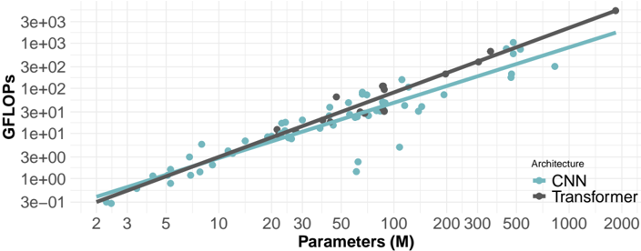Figure 1: Relation between the number of parameters and FLOPs (both axes are logarithmic). <details> <summary>Image 1 Details</summary>  ### Visual Description ## Scatter Plot: GFLOPS vs. Parameters for CNN and Transformer Architectures ### Overview The image is a scatter plot comparing the performance (GFLOPS) of Convolutional Neural Networks (CNN) and Transformer architectures against the number of parameters (in millions). Both axes are logarithmically scaled. The plot shows a general trend of increasing GFLOPS with increasing parameters for both architectures, with Transformer models generally achieving higher GFLOPS for a given number of parameters compared to CNNs. ### Components/Axes * **X-axis:** Parameters (M), logarithmically scaled from approximately 2 to 2000. Axis markers are present at 2, 3, 5, 10, 20, 30, 50, 100, 200, 300, 500, 1000, and 2000. * **Y-axis:** GFLOPS, logarithmically scaled from approximately 3e-01 (0.3) to 3e+03 (3000). Axis markers are present at 3e-01, 1e+00, 3e+00, 1e+01, 3e+01, 1e+02, 3e+02, 1e+03, and 3e+03. * **Legend:** Located in the bottom-right corner. * CNN: Represented by teal-colored data points and a teal trend line. * Transformer: Represented by dark gray data points and a dark gray trend line. ### Detailed Analysis * **CNN (Teal):** * Trend: The GFLOPS generally increase with the number of parameters. * Data Points: * At 2M parameters, GFLOPS is approximately 0.3. * At 10M parameters, GFLOPS is approximately 3. * At 50M parameters, GFLOPS ranges from 5 to 20. * At 200M parameters, GFLOPS is approximately 50. * At 1000M parameters, GFLOPS is approximately 200. * **Transformer (Dark Gray):** * Trend: The GFLOPS generally increase with the number of parameters. * Data Points: * At 2M parameters, GFLOPS is approximately 0.3. * At 10M parameters, GFLOPS is approximately 5. * At 50M parameters, GFLOPS ranges from 10 to 30. * At 200M parameters, GFLOPS is approximately 100. * At 1000M parameters, GFLOPS is approximately 500. ### Key Observations * For a given number of parameters, Transformer models tend to achieve higher GFLOPS compared to CNN models. * Both CNN and Transformer architectures exhibit a positive correlation between the number of parameters and GFLOPS. * There is some scatter in the data, indicating that factors other than the number of parameters also influence GFLOPS. ### Interpretation The scatter plot suggests that Transformer architectures are generally more efficient in terms of GFLOPS per parameter compared to CNNs. This could be attributed to the architectural differences between the two, such as the attention mechanism in Transformers, which allows for more efficient information processing. The positive correlation between parameters and GFLOPS indicates that increasing the model size generally leads to improved performance, but the scatter suggests that architectural choices and other factors play a significant role. The logarithmic scaling of both axes highlights the exponential relationship between model size and performance. </details> Despite this, Fig. 1 shows a linear relation between FLOPs and parameters. We attribute this to the balanced scaling of w , d and r . These dimensions are usually scaled together with bigger CNNs using higher resolution. Note that recent transformer models [Vaswani et al., 2017] do not follow the growth relation presented above. However, the correlation between the number of parameters and FLOPs for CNNs is 0.772 and the correlation for transformers is 0.994 (Fig. 1). This suggests that usually in both architectures parameters and FLOPs scale in tandem. We will use FLOPs, as they allow us to estimate the needed energy relating hardware FLOPS with required FLOPs for a model [Hollemans, 2018, Clark et al., 2020]. 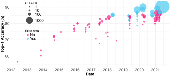## Performance and Compute There has been very significant progress for ImageNet. In 2012, AlexNet achieved 56% Top-1 accuracy (single model, one crop). In 2021, Meta Pseudo Labels (EfficientNet-L2) achieved 90.2% Top-1 accuracy (single model, one crop). However, this increase in accuracy comes with an increase in the required FLOPs for a forward pass. A forward pass for AlexNet is 1.42 GFLOPs while for EfficientNet-L2 is 1040 GFLOPs (details in the appendix). Fig. 2 shows the evolution from 2012 to 2021 in ImageNet accuracy (with the size of the bubbles representing the FLOPs of one forward pass). In recent papers some researchers began using more data than those available in ImageNet1k for training the models. However, using extra data only affects training FLOPs, but does not affect the computational cost for inferring each classification (forward pass). 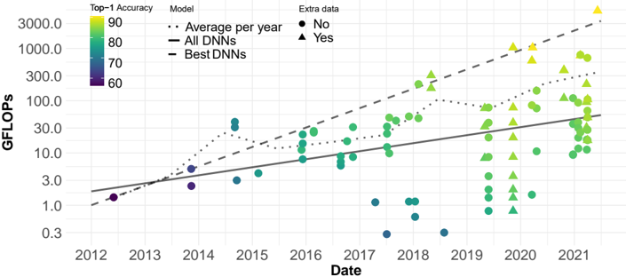If we only look at models with the best accuracy for each year we can see an exponential growth in compute (measured in FLOPs). This can be observed clearly in Fig. 3: the dashed line represents an exponential growth (shown as a linear fit since the y -axis is logarithmic). The line is fitted with Figure 2: Accuracy evolution over the years. The size of the balls represent the GFLOPs of one forward pass. <details> <summary>Image 2 Details</summary>  ### Visual Description ## Scatter Plot: Top-1 Accuracy vs. Date ### Overview The image is a scatter plot showing the relationship between Top-1 Accuracy (in percentage) and Date (from 2012 to 2021). The size of each data point represents GFLOPs, and the color indicates whether "Extra data" was used (Yes/No). ### Components/Axes * **X-axis:** Date, ranging from 2012 to 2021. * **Y-axis:** Top-1 Accuracy (%), ranging from 60% to 90%. * **Data Points:** Each point represents a data entry, with its position determined by date and accuracy. * **Size Legend (Top-Left):** * Smallest circle: 1 GFLOPs * Small circle: 10 GFLOPs * Medium circle: 100 GFLOPs * Largest circle: 1000 GFLOPs * **Color Legend (Left):** * Pink: No (Extra data) * Light Blue: Yes (Extra data) ### Detailed Analysis * **General Trend:** The Top-1 Accuracy generally increases over time from 2012 to 2021. * **2012:** One data point at approximately (2012, 56%), pink, very small size (close to 1 GFLOP). * **2013:** No data points. * **2014:** Three data points, all pink (No extra data). The accuracy values are approximately 60%, 63%, and 70%. The GFLOPs are small. * **2015:** Two data points, both pink. Accuracy values are around 73% and 78%. The GFLOPs are small. * **2016:** Several pink data points, with accuracy ranging from 75% to 80%. The GFLOPs are small. * **2017:** Several pink data points, with accuracy ranging from 80% to 85%. The GFLOPs are small. * **2018:** Several data points, mostly pink, with accuracy ranging from 82% to 86%. One light blue data point (Yes to extra data) with accuracy around 85%. The GFLOPs are small. * **2019:** A mix of pink and light blue data points. Accuracy values are generally above 80%. The GFLOPs are small. * **2020:** A cluster of pink and light blue data points, with accuracy ranging from 83% to 90%. The GFLOPs vary from small to large. * **2021:** A cluster of pink and light blue data points, with accuracy ranging from 80% to 90%. The GFLOPs vary from small to large. ### Key Observations * Accuracy generally increases over time. * The use of "Extra data" (light blue points) becomes more prevalent in later years (2019-2021). * Higher GFLOPs (larger circles) are more common in the later years (2020-2021), and they tend to correlate with higher accuracy. * There's a noticeable jump in accuracy between 2014 and 2016. ### Interpretation The scatter plot suggests that Top-1 Accuracy has improved over time, likely due to advancements in technology and the use of "Extra data." The size of the data points, representing GFLOPs, indicates that increased computational power also contributes to higher accuracy. The clustering of data points in the later years suggests a saturation point in accuracy improvement, where further gains may require significantly more computational resources or different approaches. The "Extra data" seems to have a positive impact on accuracy, especially in recent years. </details> Figure 3: GFLOPs over the years. The dashed line is a linear fit (note the logarithmic y -axis) for the models with highest accuracy per year. The solid line includes all points. <details> <summary>Image 3 Details</summary>  ### Visual Description ## Scatter Plot: DNN Performance Over Time ### Overview The image is a scatter plot showing the performance of Deep Neural Networks (DNNs) over time, measured in GFLOPS (Giga Floating Point Operations Per Second). The plot visualizes the relationship between date (from 2012 to 2021), performance, and Top-1 Accuracy, with additional data points indicating whether extra data was used. ### Components/Axes * **X-axis:** Date, ranging from 2012 to 2021 in yearly increments. * **Y-axis:** GFLOPS (Giga Floating Point Operations Per Second), ranging from 0.3 to 3000.0 on a logarithmic scale. * **Color Legend (Top-1 Accuracy):** * 90: Yellow * 80: Light Green * 70: Dark Green/Teal * 60: Purple * **Model Legend:** * Average per year: Dotted line * All DNNs: Solid line * Best DNNs: Dashed line * **Extra Data Legend:** * No: Circle marker * Yes: Triangle marker ### Detailed Analysis * **Data Points:** Each data point represents a DNN model. The color of the point indicates its Top-1 Accuracy, and the shape indicates whether extra data was used. * **Average per year (Dotted Line):** This line shows the average GFLOPS for each year. It starts at approximately 1 GFLOPS in 2012 and increases to approximately 300 GFLOPS in 2021. * 2012: ~1 GFLOPS, Accuracy ~60 * 2014: ~4 GFLOPS, Accuracy ~60 * 2015: ~30 GFLOPS, Accuracy ~70 * 2016: ~15 GFLOPS, Accuracy ~70 * 2017: ~20 GFLOPS, Accuracy ~70 * 2018: ~40 GFLOPS, Accuracy ~70 * 2019: ~50 GFLOPS, Accuracy ~70 * 2020: ~100 GFLOPS, Accuracy ~80 * 2021: ~300 GFLOPS, Accuracy ~80 * **All DNNs (Solid Line):** This line represents the trend of all DNNs. It starts at approximately 1 GFLOPS in 2012 and increases to approximately 60 GFLOPS in 2021. * 2012: ~1 GFLOPS, Accuracy ~60 * 2014: ~2 GFLOPS, Accuracy ~60 * 2016: ~4 GFLOPS, Accuracy ~70 * 2018: ~10 GFLOPS, Accuracy ~70 * 2020: ~30 GFLOPS, Accuracy ~80 * 2021: ~60 GFLOPS, Accuracy ~80 * **Best DNNs (Dashed Line):** This line represents the trend of the best-performing DNNs. It starts at approximately 1 GFLOPS in 2012 and increases to approximately 1000 GFLOPS in 2021. * 2012: ~1 GFLOPS, Accuracy ~60 * 2014: ~3 GFLOPS, Accuracy ~60 * 2016: ~10 GFLOPS, Accuracy ~70 * 2018: ~50 GFLOPS, Accuracy ~70 * 2020: ~300 GFLOPS, Accuracy ~80 * 2021: ~1000 GFLOPS, Accuracy ~90 * **Extra Data:** The use of extra data (triangle markers) appears more frequently in later years (2019-2021) and is associated with higher GFLOPS and Top-1 Accuracy. ### Key Observations * There is a clear upward trend in GFLOPS over time for all three model types (Average, All DNNs, Best DNNs). * The "Best DNNs" consistently outperform "All DNNs" and the "Average per year." * Higher Top-1 Accuracy (yellow/green) is generally associated with higher GFLOPS and later years. * The use of extra data seems to correlate with higher performance and accuracy. * The spread of data points increases over time, indicating a wider range of DNN performance. ### Interpretation The data suggests a significant improvement in DNN performance (GFLOPS) and accuracy over the period from 2012 to 2021. The "Best DNNs" show the most dramatic increase, indicating advancements in model architecture or training techniques. The correlation between the use of extra data and higher performance suggests that data augmentation or larger datasets contribute to better results. The increasing spread of data points in later years could indicate a diversification of DNN applications and architectures, leading to a wider range of performance levels. Overall, the plot demonstrates the rapid progress in the field of deep learning over the past decade. </details> the models with highest accuracy for each year. However not all models released in the latest years need so much compute. This is reflected by the solid line, which includes all points. We also see that for the same number of FLOPs we have models with increasing accuracy as time goes by. In Table 1 there is a list of models having similar number of FLOPs as AlexNet. In 2019 we have a model (EfficientNet-B1) with the same number of operations as AlexNet achieving a Top-1 accuracy of 79.1% without using extra data, and a model (NoisyStudent-B1) achieving Top-1 accuracy of 81.5% using extra data. In a period of 7 years, we have models with similar computation with much higher accuracy. We observe that when a SOTA model is released it usually has a huge number of FLOPs, and therefore consumes a large amount of energy, but in a couple of years there is a model with similar accuracy but with much lower number of FLOPs. These models are usually those that become popular in many industry applications. This observation confirms that better results for DNN models of general use are in part attributable to algorithmic improvements and not only to the use of more computing power. 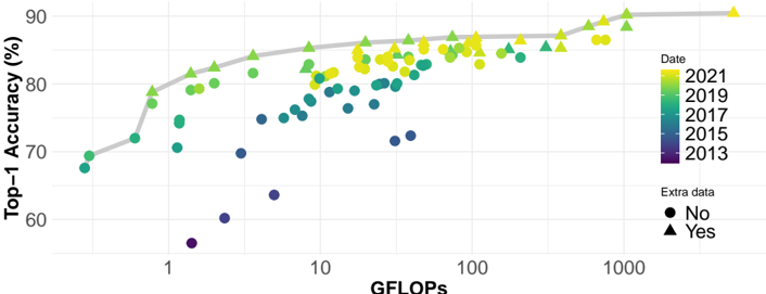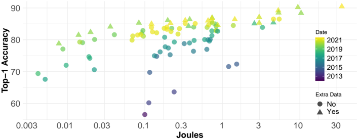Finally, Fig. 4 shows that the Pareto frontier (in grey) is composed of new models (in yellow and green), whereas old models (in purple and dark blue) are relegated below the Pareto. As expected, the models which use extra data are normally those forming the Pareto frontier. Let us note again that extra training data does not affect inference GFLOPs. | Model | Top-1 Accuracy | GFLOPs | Year | |----------------------------------------|------------------|----------|--------| | AlexNet [Krizhevsky et al., 2012] | 56.52 | 1.42 | 2012 | | ZFNet [Zeiler and Fergus, 2013] | 60.21 | 2.34 | 2013 | | GoogleLeNet [Szegedy et al., 2014] | 69.77 | 3 | 2014 | | MobileNet [Howard et al., 2017] | 70.6 | 1.14 | 2017 | | MobileNetV2 1.4 [Sandler et al., 2019] | 74.7 | 1.18 | 2018 | | EfficientNet-B1 [Tan and Le, 2020] | 79.1 | 1.4 | 2019 | | NoisyStudent-B1 [Xie et al., 2020] | 81.5 | 1.4 | 2019 | Table 1: Results for several DNNs with a similar number of FLOPs as AlexNet. <details> <summary>Image 4 Details</summary>  ### Visual Description ## Scatter Plot: Top-1 Accuracy vs. GFLOPS ### Overview The image is a scatter plot showing the relationship between Top-1 Accuracy (in percentage) and GFLOPS (floating-point operations per second) for different models, categorized by date (2013-2021) and whether extra data was used. The x-axis (GFLOPS) is on a logarithmic scale. A gray line connects the "Yes" data points, showing the trend of accuracy with increasing GFLOPS when extra data is used. ### Components/Axes * **X-axis:** GFLOPS (floating-point operations per second). Logarithmic scale with markers at 1, 10, 100, and 1000. * **Y-axis:** Top-1 Accuracy (%). Linear scale with markers at 60, 70, 80, and 90. * **Legend (Top-Right):** * **Date:** Categorizes data points by year, with colors ranging from dark purple (2013) to yellow (2021). * 2021: Yellow * 2019: Green * 2017: Teal * 2015: Blue * 2013: Purple * **Extra data:** Indicates whether extra data was used in the model. * No: Black circle * Yes: Black triangle * **Trend Line:** A gray line connects the "Yes" data points, showing the trend of accuracy with increasing GFLOPS when extra data is used. ### Detailed Analysis * **Data Points:** Each point represents a model, with its position determined by its GFLOPS and Top-1 Accuracy. The color indicates the year, and the shape (circle or triangle) indicates whether extra data was used. * **Trend Line:** The gray line connects the "Yes" (triangle) data points, showing the general trend of accuracy increasing with GFLOPS. **Specific Data Points and Trends:** * **2013 (Purple):** * "No Extra Data" (Circle): Points are clustered at the lower left of the chart, with GFLOPS values around 1 and accuracy ranging from approximately 55% to 70%. * No "Yes Extra Data" points are visible for 2013. * **2015 (Blue):** * "No Extra Data" (Circle): Points are clustered between 1 and 10 GFLOPS, with accuracy ranging from approximately 70% to 75%. * No "Yes Extra Data" points are visible for 2015. * **2017 (Teal):** * "No Extra Data" (Circle): Points are clustered between 1 and 10 GFLOPS, with accuracy ranging from approximately 75% to 80%. * "Yes Extra Data" (Triangle): Points are clustered around 1 GFLOPS, with accuracy around 80%. * **2019 (Green):** * "No Extra Data" (Circle): Points are scattered between 1 and 100 GFLOPS, with accuracy ranging from approximately 75% to 85%. * "Yes Extra Data" (Triangle): Points are scattered between 1 and 100 GFLOPS, with accuracy ranging from approximately 80% to 85%. * **2021 (Yellow):** * "No Extra Data" (Circle): Points are scattered between 10 and 1000 GFLOPS, with accuracy ranging from approximately 80% to 90%. * "Yes Extra Data" (Triangle): Points are scattered between 10 and 1000 GFLOPS, with accuracy ranging from approximately 85% to 90%. * **Trend Line (Gray):** * Starts at approximately (0.5 GFLOPS, 68% Accuracy). * Increases to approximately (1 GFLOPS, 78% Accuracy). * Increases to approximately (2 GFLOPS, 82% Accuracy). * Increases to approximately (5 GFLOPS, 83% Accuracy). * Increases to approximately (10 GFLOPS, 84% Accuracy). * Increases to approximately (100 GFLOPS, 86% Accuracy). * Increases to approximately (500 GFLOPS, 88% Accuracy). * Increases to approximately (1000 GFLOPS, 88% Accuracy). ### Key Observations * **Accuracy Increase Over Time:** The general trend is that models from later years (2019, 2021) tend to have higher accuracy for a given GFLOPS value compared to models from earlier years (2013, 2015). * **GFLOPS and Accuracy:** There is a positive correlation between GFLOPS and accuracy, especially when extra data is used, as indicated by the gray trend line. * **Impact of Extra Data:** Models using extra data (triangles) tend to have slightly higher accuracy compared to models without extra data (circles) for a given GFLOPS value. * **Saturation:** The trend line suggests that the accuracy gains from increasing GFLOPS diminish at higher GFLOPS values. ### Interpretation The scatter plot illustrates the evolution of model accuracy in relation to computational power (GFLOPS) over time. The data suggests that advancements in model architecture and training techniques (represented by the year) have led to improved accuracy for a given level of computational power. The use of extra data also contributes to higher accuracy. The trend line indicates that increasing GFLOPS leads to higher accuracy, but the gains diminish as GFLOPS increases, suggesting a point of diminishing returns. The clustering of data points for each year and data type provides insights into the typical performance characteristics of models developed during those periods. </details> GFLOPs Figure 4: Relation between accuracy and GFLOPs. ## Natural Language Analysis In this section, we analyse the trends in performance and inference compute for NLP models. To analyse performance we use GLUE, which is a popular benchmark for natural language understanding, one key task in NLP. The GLUE benchmark 4 is composed of nine sentence understanding tasks, which cover a broad range of domains. The description of each task can be found in [Wang et al., 2019]. 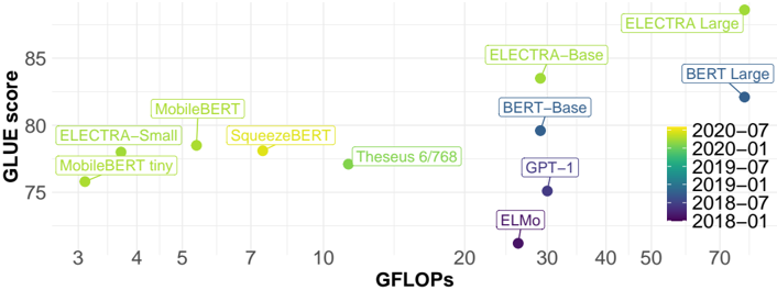## Performance and Compute We represent the improvement on the GLUE score in relation to GFLOPs over the years in Fig. 5 (and in Fig. 15 in the Appendix). GFLOPs are for single input of length 128, which is a reasonable sequence length for many use cases, being able to fit text messages or short emails. We can observe a very similar evolution to the evolution observed in ImageNet: SOTA models require a large number of FLOPs, but in a short period of time other models appear, which require much fewer FLOPs to reach the same score. There are many models that focus on being efficient instead of reaching high score, and this is reflected in their names too (e.g., MobileBERT [Sun et al., 2020] and SqueezeBERT [Iandola et al., 2020]). We note that the old models become inefficient (they have lower score with higher number of GLOPs) compared to the new ones, as it happens in CV models. 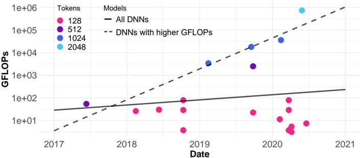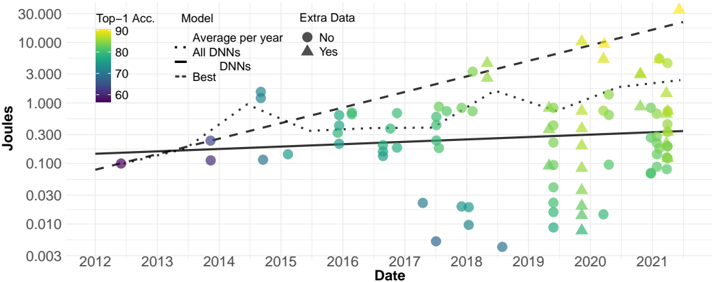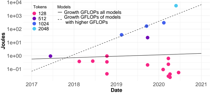## Compute Trend In Fig. 6 we include all models (regardless of having performance results) for which we found inference FLOPs estimation. The dashed line adjusts to the models with higher GFLOPs (models that, when released, become the most demanding model) and the solid line to all NLP models. In this plot we indicate the input sequence length, because in this plot we represent models with different input sequence lengths. We observe a similar trend as in CV: the GFLOPS of the most cutting-edge models have a clear exponential growth, while the general trend, i.e., considering all models, does not scale so aggressively. Actually, there is a good pocket of low-compute models in the last year. 4 Many recent models are evaluated on SUPERGLUE, but we choose GLUE to have a temporal window for our analysis. Figure 5: GFLOPs per token analysis for NLP models. <details> <summary>Image 5 Details</summary>  ### Visual Description ## Scatter Plot: GLUE Score vs. GFLOPS for Various Language Models ### Overview The image is a scatter plot comparing the GLUE (General Language Understanding Evaluation) score of various language models against their GFLOPS (billions of floating point operations per second). The data points are color-coded by the year and month of the model's release, ranging from 2018-01 to 2020-07. The plot illustrates the trade-off between model performance (GLUE score) and computational cost (GFLOPS). ### Components/Axes * **X-axis:** GFLOPS (billions of floating point operations per second). Scale ranges from 3 to 70, with tick marks at 3, 4, 5, 7, 10, 20, 30, 40, 50, and 70. * **Y-axis:** GLUE score. Scale ranges from 75 to 85, with tick marks at 75, 80, and 85. * **Data Points:** Each data point represents a language model. The position of the point indicates its GFLOPS and GLUE score. * **Labels:** Each data point is labeled with the name of the language model. * **Legend:** Located on the right side of the plot. The color gradient represents the release date of the models, ranging from dark purple (2018-01) to bright yellow (2020-07). The legend entries are: * 2020-07 (Yellow) * 2020-01 (Light Green) * 2019-07 (Green) * 2019-01 (Teal) * 2018-07 (Blue) * 2018-01 (Dark Purple) ### Detailed Analysis * **MobileBERT tiny:** Located at approximately (3, 76). Color is light green, corresponding to approximately 2020-01. * **ELECTRA-Small:** Located at approximately (4, 78). Color is light green, corresponding to approximately 2020-01. * **MobileBERT:** Located at approximately (5.5, 79). Color is light green, corresponding to approximately 2020-01. * **SqueezeBERT:** Located at approximately (7, 78.5). Color is yellow-green, corresponding to approximately 2020-04. * **Theseus 6/768:** Located at approximately (11, 77). Color is green, corresponding to approximately 2019-07. * **ELMo:** Located at approximately (27, 72). Color is dark purple, corresponding to approximately 2018-01. * **GPT-1:** Located at approximately (29, 75). Color is purple-blue, corresponding to approximately 2018-07. * **BERT-Base:** Located at approximately (32, 79.5). Color is blue, corresponding to approximately 2018-07. * **ELECTRA-Base:** Located at approximately (37, 83). Color is light green, corresponding to approximately 2020-01. * **ELECTRA Large:** Located at approximately (52, 86). Color is yellow-green, corresponding to approximately 2020-04. * **BERT Large:** Located at approximately (68, 83). Color is blue, corresponding to approximately 2018-07. ### Key Observations * There is a general trend of increasing GLUE score with increasing GFLOPS. * Models released later (closer to 2020-07) tend to have higher GLUE scores for a given GFLOPS value, suggesting improvements in model efficiency over time. * The ELECTRA models (Small, Base, and Large) show a clear progression in both GFLOPS and GLUE score. * The BERT models (Base and Large) also show a progression, but they are older than the ELECTRA models. * MobileBERT and SqueezeBERT are designed for efficiency, achieving relatively high GLUE scores with lower GFLOPS. ### Interpretation The scatter plot illustrates the trade-off between model performance (GLUE score) and computational cost (GFLOPS) for various language models. The color-coding by release date reveals a trend of improving model efficiency over time, as newer models tend to achieve higher GLUE scores for a given GFLOPS value. This suggests that advancements in model architecture and training techniques are enabling researchers to develop more efficient and performant language models. The plot also highlights the existence of models like MobileBERT and SqueezeBERT, which prioritize efficiency and achieve relatively high GLUE scores with lower computational requirements. The data suggests that the field of NLP is continuously evolving, with a focus on developing models that are both accurate and computationally efficient. </details> Figure 6: GFLOPs per token analysis for NLP models. <details> <summary>Image 6 Details</summary>  ### Visual Description ## Scatter Plot: GFLOPS vs. Date for Different DNN Models and Token Sizes ### Overview The image is a scatter plot showing the relationship between GFLOPS (floating point operations per second) and date for different deep neural network (DNN) models, categorized by token size. The plot includes trend lines for "All DNNs" and "DNNs with higher GFLOPS." ### Components/Axes * **X-axis:** Date, ranging from 2017 to 2021. * **Y-axis:** GFLOPS, on a logarithmic scale from 1e+01 (10) to 1e+06 (1,000,000). * **Legend (Top-Left):** * **Tokens:** * Pink: 128 * Purple: 512 * Blue: 1024 * Light Blue: 2048 * **Models:** * Solid Black Line: All DNNs * Dashed Black Line: DNNs with higher GFLOPs ### Detailed Analysis * **All DNNs (Solid Black Line):** This line shows a slight upward trend. * Approximate GFLOPS in 2017: 50 * Approximate GFLOPS in 2021: 200 * **DNNs with higher GFLOPs (Dashed Black Line):** This line shows a significant upward trend. * Approximate GFLOPS in 2017: 2 * Approximate GFLOPS in 2021: 500,000 * **Token Size 128 (Pink):** The data points are clustered around the GFLOPS range of 10 to 100, primarily in 2020. * 2018: ~30 GFLOPS * 2019: ~30 GFLOPS * 2020: Multiple points between ~2 and ~100 GFLOPS * **Token Size 512 (Purple):** There are two data points. * 2017: ~60 GFLOPS * 2019: ~3000 GFLOPS * **Token Size 1024 (Blue):** The data points show an upward trend. * 2019: ~5000 GFLOPS * 2020: ~20000 GFLOPS * **Token Size 2048 (Light Blue):** There is one data point. * 2020: ~800000 GFLOPS ### Key Observations * GFLOPS generally increase with date for DNNs with higher GFLOPS. * Token size appears to correlate with higher GFLOPS, with larger token sizes generally appearing higher on the plot. * The "All DNNs" trend line shows a much slower increase in GFLOPS compared to "DNNs with higher GFLOPs." * The majority of the 128 token data points are clustered in 2020, with relatively low GFLOPS. ### Interpretation The plot suggests that DNNs with higher GFLOPS have experienced significant performance improvements over time. The token size also appears to play a role in GFLOPS, with larger token sizes associated with higher computational performance. The difference between the "All DNNs" and "DNNs with higher GFLOPs" trend lines indicates that a subset of DNNs is driving the overall increase in GFLOPS. The clustering of 128 token data points in 2020 with lower GFLOPS may indicate a focus on smaller, more efficient models during that period, or simply a larger number of models with that token size being developed. The single 2048 token data point in 2020 shows a very high GFLOPS, suggesting a significant leap in performance for models using that token size. </details> ## Hardware Progress We use FLOPS as a measure of hardware performance and FLOPS/Watt as a measure of hardware efficiency. We collected performance for different precision formats and tensor cores for a wide range of GPUs. The results are shown in Fig. 7. Note that the y -axis is in logarithmic scale. Theoretical FLOPS for tensor cores are very high in the plot. However, the actual performance for inference using tensor cores is not so high, if we follow a more realistic estimation for the Nvidia GPUs (V100, A100 and T4 5 ). The details of this estimation are shown in Table 3 in the appendix. Figure 7: Theoretical Nvidia GPUs GFLOPS per Watt. Data in Table 8 in the appendix. <details> <summary>Image 7 Details</summary>  ### Visual Description ## Scatter Plot: GFLOPs/Watt vs. Date for Different Precision Levels ### Overview The image is a scatter plot showing the relationship between GFLOPs/Watt (performance per watt) and Date (year) for three different precision levels: FP16, FP16/FP32 Tensor, and FP32. The plot illustrates how performance per watt has changed over time for each precision level. ### Components/Axes * **Title:** None explicitly present in the image. * **X-axis:** * Label: "Date" * Scale: Years from 2011 to 2021 in increments of 1 year. * **Y-axis:** * Label: "GFLOPs/Watt" * Scale: Logarithmic scale from 7 to 1000. Major tick marks are at 7, 10, 20, 30, 50, 70, 100, 200, 300, 500, 700, and 1000. * **Legend (Top-Left):** * "Precision" * Black circle: "FP16" * Light Blue circle: "FP16/FP32 Tensor" * Yellow circle: "FP32" ### Detailed Analysis **FP32 (Yellow):** * **Trend:** Generally increasing over time. * **Data Points:** * 2011: ~7 GFLOPs/Watt * 2012: ~15 GFLOPs/Watt * 2013: ~17 GFLOPs/Watt * 2014: ~22 GFLOPs/Watt * 2015: ~23 GFLOPs/Watt * 2016: ~28 GFLOPs/Watt * 2017: ~35 GFLOPs/Watt * 2018: ~40 GFLOPs/Watt * 2019: ~45 GFLOPs/Watt * 2020: ~55 GFLOPs/Watt * 2021: ~70 GFLOPs/Watt **FP16 (Black):** * **Trend:** Data only available from 2016 onwards. Performance increases, then plateaus, and then increases again. * **Data Points:** * 2016: ~75 GFLOPs/Watt * 2018: ~100 GFLOPs/Watt * 2019: ~110 GFLOPs/Watt * 2020: ~210 GFLOPs/Watt * 2021: ~110 GFLOPs/Watt **FP16/FP32 Tensor (Light Blue):** * **Trend:** Data only available from 2018 onwards. Performance increases sharply and then decreases. * **Data Points:** * 2018: ~250 GFLOPs/Watt * 2019: ~450 GFLOPs/Watt * 2020: ~250 GFLOPs/Watt ### Key Observations * FP32 performance per watt shows a consistent, gradual increase over the entire period from 2011 to 2021. * FP16 and FP16/FP32 Tensor data are only available from 2018 onwards. * FP16/FP32 Tensor achieves the highest performance per watt, peaking around 2019. * FP16 performance per watt shows a significant jump in 2020. ### Interpretation The plot demonstrates the evolution of performance per watt for different floating-point precision levels. The consistent increase in FP32 performance suggests ongoing improvements in hardware and software optimization for this standard precision. The introduction and subsequent performance of FP16 and FP16/FP32 Tensor indicate a shift towards lower-precision computing to achieve higher performance per watt, particularly for specialized tasks like tensor operations. The peak in FP16/FP32 Tensor performance around 2019, followed by a decrease, could be attributed to changes in hardware architectures or software optimization strategies. The jump in FP16 performance in 2020 suggests a renewed focus on optimizing this precision level. Overall, the data highlights the trade-offs between precision and energy efficiency in computing. </details> 5 Specifications in: https://www.nvidia.com/en-us/data-center/. 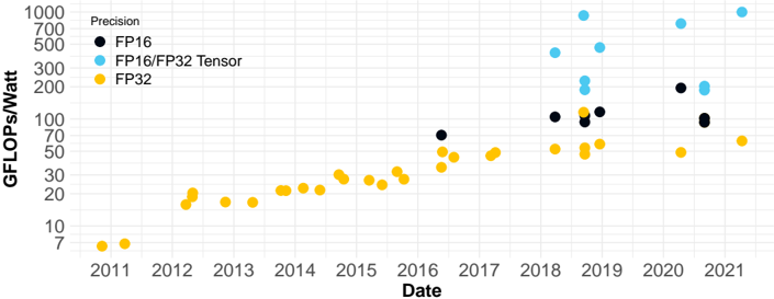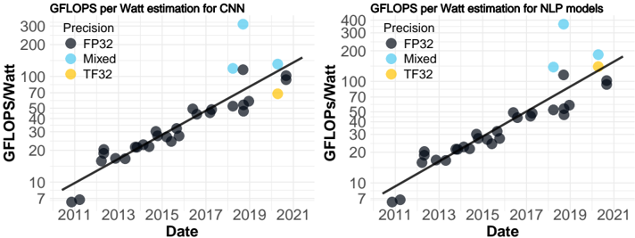With these estimations we obtained good linear fits (with the y -axis in logarithmic scale) to each data set, one for CV and another for NLP, as shown by the solid lines in Fig. 8. Notice that there is a particular point in Fig. 8 for year 2018 that stands out among the others by a large margin. This corresponds to T4 using mixed precision, a GPU specifically designed for inference, and this is the reason why it is so efficient for this task. Figure 8: Nvidia GPU GFLOPS per Watt adapted for CV (CNNs) and NLP models. Data in Table 9 in the appendix. <details> <summary>Image 8 Details</summary>  ### Visual Description ## Scatter Plots: GFLOPS per Watt Estimation for CNN and NLP Models ### Overview The image contains two scatter plots comparing GFLOPS per Watt estimation for CNN (Convolutional Neural Networks) and NLP (Natural Language Processing) models. Each plot shows data points representing different precision levels (FP32, Mixed, and TF32) over time (2011-2021). A trend line is included on each plot. ### Components/Axes **Left Plot (CNN):** * **Title:** GFLOPS per Watt estimation for CNN * **Y-axis:** GFLOPS/Watt (labeled with values 7, 10, 20, 30, 40, 50, 70, 100, 200, 300) * **X-axis:** Date (labeled with years 2011, 2013, 2015, 2017, 2019, 2021) * **Legend (Top-Left):** * FP32 (Dark Gray) * Mixed (Light Blue) * TF32 (Yellow) **Right Plot (NLP):** * **Title:** GFLOPS per Watt estimation for NLP models * **Y-axis:** GFLOPS/Watt (labeled with values 7, 10, 20, 30, 40, 50, 70, 100, 200, 300, 400) * **X-axis:** Date (labeled with years 2011, 2013, 2015, 2017, 2019, 2021) * **Legend (Top-Left):** * FP32 (Dark Gray) * Mixed (Light Blue) * TF32 (Yellow) ### Detailed Analysis **Left Plot (CNN):** * **FP32 (Dark Gray):** The majority of the data points are FP32. The trend is generally upward, indicating increasing GFLOPS/Watt over time. * 2011: ~7 GFLOPS/Watt * 2013: ~15 GFLOPS/Watt * 2015: ~22 GFLOPS/Watt * 2017: ~35 GFLOPS/Watt * 2019: ~50 GFLOPS/Watt * 2021: ~65 GFLOPS/Watt * **Mixed (Light Blue):** There are two Mixed precision data points. * 2019: ~180 GFLOPS/Watt * 2020: ~350 GFLOPS/Watt * **TF32 (Yellow):** There is one TF32 data point. * 2020: ~75 GFLOPS/Watt **Right Plot (NLP):** * **FP32 (Dark Gray):** The majority of the data points are FP32. The trend is generally upward, indicating increasing GFLOPS/Watt over time. * 2011: ~7 GFLOPS/Watt * 2013: ~15 GFLOPS/Watt * 2015: ~20 GFLOPS/Watt * 2017: ~30 GFLOPS/Watt * 2019: ~50 GFLOPS/Watt * 2021: ~70 GFLOPS/Watt * **Mixed (Light Blue):** There is one Mixed precision data point. * 2019: ~200 GFLOPS/Watt * **TF32 (Yellow):** There is one TF32 data point. * 2020: ~120 GFLOPS/Watt ### Key Observations * Both CNN and NLP models show an increasing trend in GFLOPS/Watt over time for FP32 precision. * Mixed precision generally achieves higher GFLOPS/Watt compared to FP32 and TF32. * The NLP plot has a higher maximum GFLOPS/Watt value (400) compared to the CNN plot (300). * The trend lines on both plots appear to be linear. ### Interpretation The data suggests that the energy efficiency of both CNN and NLP models has been improving over time, as indicated by the increasing GFLOPS/Watt. The use of mixed precision can significantly boost performance per watt. The difference in the Y-axis scale between the two plots suggests that NLP models may have the potential for higher energy efficiency compared to CNN models. The single data points for Mixed and TF32 precision make it difficult to draw definitive conclusions about their trends, but they indicate that these precisions can offer significant performance gains in certain years. </details> ## Energy Consumption Analysis Once we have estimated the inference FLOPs for a range of models and the GFLOPS per Watt for different GPUs, we can estimate the energy (in Joules) consumed in one inference. We do this by dividing the FLOPs for the model by FLOPS per Watt for the GPU. But how can we choose the FLOPS per Watt that correspond to the model? We use the models presented in Fig. 8 to obtain an estimation of GLOPS per Watt for the model's release date . In this regard, Henderson et al. (2020) report that FLOPs for DNNs can be misleading sometimes, due to underlying optimisations at the firmware, frameworks, memory and hardware that can influence energy efficiency. They show that energy and FLOPs are highly correlated for the same architecture, but the correlation decreases when different architectures are mixed. We consider that this low correlation does not affect our estimations significantly as we analyse the trends through the years and we fit in the exponential scale, where dispersion is reduced. To perform a more precise analysis it would be necessary to measure power consumption for each network with the original hardware and software, as unfortunately the required energy per (one) inference is rarely reported. <details> <summary>Image 9 Details</summary>  ### Visual Description ## Scatter Plot: Energy Consumption of DNNs Over Time ### Overview The image is a scatter plot showing the energy consumption (in Joules) of Deep Neural Networks (DNNs) over time (from 2012 to 2021). The plot includes data points for individual DNNs, as well as trend lines representing the average energy consumption per year and the energy consumption of the "best" DNNs. The color of each data point indicates the Top-1 Accuracy of the model, ranging from purple (60) to yellow (90). The shape of the data point indicates whether extra data was used (triangle = Yes, circle = No). ### Components/Axes * **X-axis:** Date (Year), ranging from 2012 to 2021. * **Y-axis:** Joules (Energy Consumption), on a logarithmic scale from 0.003 to 30.000. * **Color Legend (Top-Left):** Top-1 Accuracy, ranging from 60 (purple) to 90 (yellow). * **Shape Legend (Top-Right):** Extra Data, with circles representing "No" and triangles representing "Yes". * **Line Legend (Top-Center):** Model, with a dotted line representing "Average per year", a solid line representing "All DNNs", and a dashed line representing "Best DNNs". ### Detailed Analysis * **Y-Axis Scale:** The Y-axis is logarithmic. The major tick marks are at 0.003, 0.010, 0.030, 0.100, 0.300, 1.000, 3.000, 10.000, and 30.000 Joules. * **Data Point Shapes:** Circles and Triangles. Circles represent "No Extra Data", Triangles represent "Yes Extra Data". * **Color Gradient:** The color of the data points represents the "Top-1 Accuracy". Purple represents 60, and Yellow represents 90. The color transitions smoothly between these values. * **Average per year (Dotted Line):** * 2012: Approximately 0.1 Joules. * 2014: Approximately 0.3 Joules. * 2017: Approximately 0.5 Joules. * 2019: Approximately 0.7 Joules. * 2021: Approximately 1.0 Joules. * Trend: The average energy consumption per year shows an upward trend, increasing from approximately 0.1 Joules in 2012 to approximately 1.0 Joules in 2021. * **All DNNs (Solid Line):** * 2012: Approximately 0.15 Joules. * 2021: Approximately 0.3 Joules. * Trend: The energy consumption of all DNNs shows a slight upward trend, increasing from approximately 0.15 Joules in 2012 to approximately 0.3 Joules in 2021. * **Best DNNs (Dashed Line):** * 2012: Approximately 0.1 Joules. * 2014: Approximately 0.2 Joules. * 2017: Approximately 0.5 Joules. * 2019: Approximately 1.0 Joules. * 2021: Approximately 10.0 Joules. * Trend: The energy consumption of the best DNNs shows a significant upward trend, increasing from approximately 0.1 Joules in 2012 to approximately 10.0 Joules in 2021. * **Individual Data Points:** * The data points are scattered across the plot, with a higher concentration of points in the later years (2018-2021). * The color of the data points generally shifts from purple/blue in the earlier years to green/yellow in the later years, indicating an increase in Top-1 Accuracy over time. * The presence of both circles and triangles in each year suggests that some DNNs used extra data while others did not. ### Key Observations * Energy consumption generally increases over time for all models. * The "Best DNNs" exhibit a much steeper increase in energy consumption compared to the average. * Top-1 Accuracy tends to increase over time, as indicated by the color gradient. * There is a wide range of energy consumption values for DNNs in any given year. * The use of extra data is prevalent throughout the years. ### Interpretation The data suggests that while the average energy consumption of DNNs has increased over time, the "best" DNNs have experienced a much more significant increase in energy consumption. This could be due to the increasing complexity and size of these models, as well as the use of more computationally intensive techniques. The increase in Top-1 Accuracy over time suggests that these more energy-intensive models are also more accurate. The scatter of data points indicates a wide variety of DNN architectures and training methods, each with its own energy consumption profile. The presence of both circles and triangles suggests that the use of extra data is not necessarily correlated with higher accuracy or lower energy consumption. Overall, the plot highlights the trade-offs between energy consumption, accuracy, and the use of extra data in DNNs. </details> Extra Data No Yes Top-1 Accuracy Lines Average per year Model all DNNs Model best DNNs Figure 9: Estimated Joules of a forward pass (CV). The dashed line is a linear fit (logarithmic y -axis) for the models with highest accuracy per year. The solid line fits all models. We can express the efficiency metric FLOPS per Watt as FLOPs per Joule, as shown in Eq. 1. Having this equivalence we can use it to divide the FLOPs needed for a forward pass and obtain the required Joules, see Eq. 2. Doing this operation we obtain the consumed energy in Joules. Figure 10: Estimated Joules of a forward pass (NLP). Same interpretation as in Fig. 9. <details> <summary>Image 10 Details</summary>  ### Visual Description ## Scatter Plot: Energy Consumption vs. Date for Different Token Sizes ### Overview The image is a scatter plot showing the relationship between energy consumption (Joules) and date for different token sizes. The plot includes data points for token sizes of 128, 512, 1024, and 2048. Trend lines indicate the growth of GFLOPs (Giga Floating Point Operations per Second) for all models and for models with higher GFLOPs. ### Components/Axes * **X-axis:** Date, ranging from 2017 to 2021. * **Y-axis:** Joules, ranging from 1e-01 (0.1) to 1e+04 (10,000) on a logarithmic scale. * **Legend (Top-Left):** * **Tokens:** * Pink: 128 * Purple: 512 * Blue: 1024 * Light Blue: 2048 * **Models:** * Solid Black Line: Growth GFLOPs all models * Dashed Black Line: Growth GFLOPs of models with higher GFLOPs ### Detailed Analysis * **Token Size 128 (Pink):** * Data points are clustered around the 2020 mark, with energy consumption values ranging approximately from 0.05 to 1 Joule. * There is a single data point around 2018 with a value of approximately 0.5 Joules. * **Token Size 512 (Purple):** * One data point in 2017 at approximately 1 Joule. * One data point in 2019 at approximately 20 Joules. * **Token Size 1024 (Blue):** * One data point in 2019 at approximately 100 Joules. * One data point in 2020 at approximately 200 Joules. * **Token Size 2048 (Light Blue):** * One data point in 2020 at approximately 8000 Joules. * **Growth GFLOPs all models (Solid Black Line):** * The line is nearly horizontal, indicating a very slight increase in GFLOPs over time. * The line starts at approximately 0.7 Joules in 2017 and ends at approximately 1.2 Joules in 2021. * **Growth GFLOPs of models with higher GFLOPs (Dashed Black Line):** * The line slopes upward, indicating an increase in GFLOPs over time. * The line starts at approximately 0.01 Joules in 2017 and ends at approximately 1000 Joules in 2021. ### Key Observations * Energy consumption generally increases with token size. * The energy consumption for smaller token sizes (128) is relatively stable over time. * The energy consumption for larger token sizes (1024, 2048) shows a significant increase in later years (2020). * The growth of GFLOPs for all models is relatively flat, while the growth of GFLOPs for models with higher GFLOPs shows a significant increase over time. ### Interpretation The data suggests that as token sizes increase, the energy consumption also increases, particularly in recent years. The flat growth of GFLOPs for all models indicates that the average computational efficiency has not improved significantly over time. However, the increasing GFLOPs for models with higher GFLOPs suggests that there is a trend towards more computationally intensive models, which consume more energy. The clustering of 128 token data points around 2020 suggests that these models were more prevalent during that period. The single data points for larger token sizes indicate that these models were less common but had significantly higher energy consumption. </details> $$E \text {efficiency} & = \frac { \text {HW Perf. } } { \text {Power} } \text { in units: } \frac { \ F L O P S } { W a t t } = \frac { \ F L O P s / s } { J o u l e s / s } = \frac { \ F L O P s } { J o u l e } & ( 1 ) \\ E \text {energy} & = \frac { \text {Fwd. Pass } } { \text {Efficiency} } \text { in units: } \frac { \ F L O P s } { \ F L O p s / J o u l e } = J o u l e$$ Applying this calculation to all collected models we obtain Fig. 9 for CV. The dashed line represents an exponential trend (a linear fit as the y -axis is logarithmic), adjusted to the models with highest accuracy for each year, like in Fig. 2, and the dotted line represent the average Joules for each year. By comparing both plots we can see that hardware progress softens the growth observed for FLOPs, but the growth is still clearly exponential for the models with high accuracy. The solid line is almost horizontal, but in a logarithmic scale this may be interpreted as having an exponential growth with a small base or a linear fit on the semi log plot that is affected by the extreme points. In Fig. 10 we do the same for NLP models and we see a similar picture. 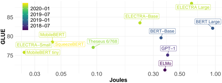Fig. 11 shows the relation between Top-1 Accuracy and Joules. Joules are calculated in the same way as in Fig. 9. The relation is similar as the observed in Fig. 4, but in Fig. 11 the older models are not only positioned further down in the y -axis (performance) but they tend to cluster on the bottom right part of the plot (high Joules), so their position on the y -axis is worse than for Fig. 4 due to the evolution in hardware. This is even more clear for NLP, as seen in Fig. 12. Figure 11: Relation between Joules and Top-1 Accuracy over the years (CV, ImageNet). <details> <summary>Image 11 Details</summary>  ### Visual Description ## Scatter Plot: Top-1 Accuracy vs. Joules ### Overview The image is a scatter plot showing the relationship between Top-1 Accuracy and Joules, with data points differentiated by date (2013, 2015, 2017, 2019, 2021) and the presence of "Extra Data" (Yes/No). The x-axis (Joules) is on a logarithmic scale. ### Components/Axes * **Title:** None explicitly present in the image. * **X-axis:** * Label: "Joules" * Scale: Logarithmic * Markers: 0.003, 0.01, 0.03, 0.1, 0.3, 1, 3, 10, 30 * **Y-axis:** * Label: "Top-1 Accuracy" * Scale: Linear * Markers: 60, 70, 80, 90 * **Legend:** Located in the top-right corner. * **Date:** * 2021: Yellow * 2019: Light Green * 2017: Green * 2015: Dark Green/Teal * 2013: Purple/Dark Blue * **Extra Data:** * No: Circle * Yes: Triangle ### Detailed Analysis The data points are scattered across the plot, with a general trend of increasing Top-1 Accuracy as Joules increase. The color of the data points indicates the year, and the shape indicates whether "Extra Data" is present. * **2013 (Purple/Dark Blue):** The data points are clustered at the lower-left of the plot, indicating lower Joules and lower Top-1 Accuracy. * At 0.1 Joules, accuracy is approximately 56% with no extra data (circle). * At 0.3 Joules, accuracy is approximately 63% with no extra data (circle). * **2015 (Dark Green/Teal):** The data points are located in the middle of the plot. * At 0.1 Joules, accuracy is approximately 70% with no extra data (circle). * At 0.3 Joules, accuracy is approximately 75% with no extra data (circle). * **2017 (Green):** The data points are located in the middle to upper-middle of the plot. * At 0.01 Joules, accuracy is approximately 69% with no extra data (circle). * At 0.03 Joules, accuracy is approximately 72% with no extra data (circle). * At 0.1 Joules, accuracy is approximately 82% with extra data (triangle). * **2019 (Light Green):** The data points are located in the upper-middle of the plot. * At 0.01 Joules, accuracy is approximately 78% with extra data (triangle). * At 0.03 Joules, accuracy is approximately 82% with extra data (triangle). * At 0.1 Joules, accuracy is approximately 83% with extra data (triangle). * **2021 (Yellow):** The data points are located in the upper-right of the plot, indicating higher Joules and higher Top-1 Accuracy. * At 0.1 Joules, accuracy is approximately 82% with extra data (triangle). * At 1 Joules, accuracy is approximately 85% with extra data (triangle). * At 10 Joules, accuracy is approximately 88% with extra data (triangle). ### Key Observations * There is a general positive correlation between Joules and Top-1 Accuracy. * The data points from later years (2019, 2021) tend to have higher Top-1 Accuracy for a given Joules value compared to earlier years (2013, 2015). * The presence of "Extra Data" (triangle markers) seems to be associated with higher Top-1 Accuracy. * The data points for 2013 are clustered at the lower end of both axes, indicating lower performance. ### Interpretation The scatter plot suggests that, over time, models have become more energy-efficient, achieving higher Top-1 Accuracy with lower Joules. The "Extra Data" likely represents additional techniques or features that improve model performance. The trend indicates advancements in model design and training methodologies, leading to better accuracy with less energy consumption. The logarithmic scale on the x-axis suggests that the relationship between Joules and Top-1 Accuracy may not be linear, and there might be diminishing returns as Joules increase. </details> ## Forecasting and Multiplicative Effect In our analysis we see that DNNs as well as hardware are improving their efficiency and do not show symptoms of standstill. This is consistent with most studies in the literature: performance will Figure 12: Relation between Joules and GLUE score over the years (NLP, GLUE). <details> <summary>Image 12 Details</summary>  ### Visual Description ## Scatter Plot: GLUE Score vs. Joules for Various Language Models ### Overview The image is a scatter plot comparing the GLUE (General Language Understanding Evaluation) score of various language models against their energy consumption in Joules. The plot visualizes the trade-off between model performance and energy efficiency. The data points are color-coded by the year and month of the model's release, ranging from 2018-07 to 2020-01. ### Components/Axes * **X-axis:** Joules (Energy Consumption). Scale ranges from 0.03 to 1.00, with markers at 0.03, 0.05, 0.10, 0.30, 0.50, and 1.00. * **Y-axis:** GLUE (General Language Understanding Evaluation) score. Scale ranges from 75 to 85, with a marker at 80. * **Legend:** Located at the top-left corner, the legend indicates the color-coding scheme for the data points based on the year and month of the model's release: * 2020-01: Light Green * 2019-07: Green * 2019-01: Blue * 2018-07: Purple ### Detailed Analysis Here's a breakdown of the data points, their approximate coordinates, and their corresponding release dates based on color: * **MobileBERT tiny:** (0.03, 75). Color: Light Green. Release Date: 2020-01 * **ELECTRA-Small:** (0.03, 78). Color: Light Green. Release Date: 2020-01 * **SqueezeBERT:** (0.05, 78). Color: Light Green. Release Date: 2020-01 * **MobileBERT:** (0.05, 80). Color: Light Green. Release Date: 2020-01 * **Theseus 6/768:** (0.10, 77). Color: Green. Release Date: 2019-07 * **ELECTRA-Base:** (0.30, 84). Color: Light Green. Release Date: 2020-01 * **BERT-Base:** (0.30, 80). Color: Blue. Release Date: 2019-01 * **GPT-1:** (0.30, 77). Color: Purple. Release Date: 2018-07 * **ELMo:** (0.30, 74). Color: Purple. Release Date: 2018-07 * **ELECTRA Large:** (0.50, 87). Color: Light Green. Release Date: 2020-01 * **BERT Large:** (1.00, 82). Color: Blue. Release Date: 2019-01 **Trend Verification:** * Models released later (2020-01, Light Green) tend to have higher GLUE scores and varying energy consumption. * Models released earlier (2018-07, Purple) have lower GLUE scores and relatively lower energy consumption. * There is a general trend of increasing GLUE score with increasing energy consumption, but there are exceptions. ### Key Observations * **Energy Efficiency:** Models like MobileBERT tiny, ELECTRA-Small, and SqueezeBERT achieve relatively good GLUE scores with very low energy consumption. * **Performance Leaders:** ELECTRA Large achieves the highest GLUE score but also has a moderate energy consumption. * **Trade-off:** There is a clear trade-off between model performance (GLUE score) and energy consumption (Joules). Some models prioritize energy efficiency, while others prioritize performance. * **Temporal Trend:** Newer models (2020-01) generally outperform older models (2018-07) in terms of GLUE score, indicating advancements in language model architectures and training techniques. ### Interpretation The scatter plot illustrates the evolution of language models, showcasing the progress in both performance and energy efficiency. The data suggests that newer models (released in 2020-01) tend to achieve higher GLUE scores, indicating improved language understanding capabilities. However, this improvement often comes at the cost of increased energy consumption. The plot highlights the importance of considering both performance and energy efficiency when selecting a language model for a specific application. Models like MobileBERT tiny and ELECTRA-Small offer a good balance between performance and energy consumption, making them suitable for resource-constrained environments. On the other hand, models like ELECTRA Large prioritize performance and may be preferred for applications where accuracy is paramount, even if it means higher energy consumption. The plot also reveals that there is no single "best" model, as the optimal choice depends on the specific requirements of the application. By visualizing the trade-off between performance and energy consumption, the scatter plot provides valuable insights for decision-making in the field of natural language processing. 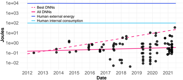</details> Figure 13: Estimated Joules per forward pass (e.g., one prediction) compared to human energy consumption in 1s (CV). <details> <summary>Image 13 Details</summary>  ### Visual Description ## Chart: Energy Consumption of DNNs vs. Humans Over Time ### Overview The image is a scatter plot showing the energy consumption (in Joules) of Deep Neural Networks (DNNs) over time (from 2012 to 2021), compared to human energy consumption. The y-axis is logarithmic, ranging from 1e-02 to 1e+04 Joules. The plot includes trend lines for "Best DNNs" and "All DNNs," as well as horizontal lines representing "Human external energy" and "Human internal consumption." ### Components/Axes * **X-axis:** Date (from 2012 to 2021) * **Y-axis:** Joules (logarithmic scale from 1e-02 to 1e+04) * **Legend (top-left):** * Best DNNs (dashed pink line) * All DNNs (solid magenta line) * Human external energy (solid blue line) * Human internal consumption (solid cyan line) ### Detailed Analysis * **Best DNNs (dashed pink line):** The trend line slopes upward, indicating an increase in energy consumption over time. * Approximate value in 2012: 1e-01 Joules * Approximate value in 2021: 2e+01 Joules * **All DNNs (solid magenta line):** The trend line is relatively flat, suggesting a stable average energy consumption. * Approximate value in 2012: 2e-01 Joules * Approximate value in 2021: 3e-01 Joules * **Human external energy (solid blue line):** A horizontal line at approximately 1e+04 Joules. * **Human internal consumption (solid cyan line):** A horizontal line at approximately 1e+02 Joules. * **Data Points (black dots):** Scattered data points represent individual DNN energy consumption values. The density of points increases significantly from 2019 to 2021. The data points are scattered between 1e-02 and 1e+01 Joules. ### Key Observations * Energy consumption of "Best DNNs" is increasing over time. * Average energy consumption of "All DNNs" remains relatively stable. * Human external energy consumption is significantly higher than DNN energy consumption. * Human internal consumption is higher than most DNN energy consumption values. * There is a significant increase in the number of DNN energy consumption data points from 2019 to 2021. ### Interpretation The chart illustrates the energy consumption trends of DNNs in comparison to human energy consumption. The increasing energy consumption of "Best DNNs" suggests that more complex and computationally intensive models are being developed. The relatively stable average energy consumption of "All DNNs" indicates that many DNNs remain energy-efficient. The comparison to human energy consumption provides context, showing that even the most energy-intensive DNNs consume significantly less energy than human external energy expenditure. The increased density of data points in recent years reflects the growing prevalence and use of DNNs. The data suggests that while the best DNNs are becoming more energy intensive, the average energy consumption of all DNNs is relatively stable, and still significantly lower than human energy consumption. </details> continue growing as compute grows, but at the same time efficiency is increasing. However, this is the first work that analyses whether these two things cancel, especially when we analyse inference and not training. Our conclusion is that they not cancel out for the cutting-edge models of each moment but this is less clear for the regular models in general use by industries and invididuals. However, since we are focusing on inference costs, we need to consider the multiplicative factor. How many inferences are performed per capita ? This has definitely increased very significantly with the use of smart devices, Internet of things and many other devices around us, which are incorporating DNN-based services. However, how many inference passes per capita do we have at this moment, and how is this growing? This is very difficult to estimate, and we leave it for future work. However, it is interesting to analyse possible hypotheses: assume there is one inference pass of a neural network application per second per capita. What would this imply in terms of energy consumption? In order to put this inference energy consumption in context we calculate the value of average human body energy consumption (we will refer to it as somatic or internal consumption) in one second and the average energy that a human being consumes in one second with all their commodities (we will refer to it as external consumption). The internal consumption is calculated assuming 2000 KCal per person day, and converting this to Joules/s, giving approximately 100 Joules/s. The external consumption is the sum of total energy consumption, including electricity, transport and heating, using the USA as a reference [Ritchie and Roser, 2020]. This suggests 79,897 Kwh/year in 2019, which is approximately 10,000 Joules every second. The comparison of these two references with the trends can be seen in Fig. 13 (CV). As we see, the energy consumed for one inference of the best models approaches the energy consumed by the human body in one second but stills far from the external energy consumed in one second. If each human did an AI-based decision implying a forward pass every second during the whole day (and night), this would be still well below their Figure 14: Estimated Joules per forward pass (e.g., one prediction) compared to human consumption in 1s (NLP). 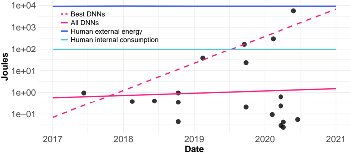<details> <summary>Image 14 Details</summary>  ### Visual Description ## Chart: Energy Consumption of DNNs vs. Humans ### Overview The image is a scatter plot showing the energy consumption of Deep Neural Networks (DNNs) over time, compared to human energy consumption. The y-axis represents energy in Joules (logarithmic scale), and the x-axis represents the date from 2017 to 2021. The plot includes data points for individual DNNs, trend lines for "Best DNNs" and "All DNNs", and horizontal lines representing "Human external energy" and "Human internal consumption". ### Components/Axes * **X-axis:** Date, ranging from 2017 to 2021. * **Y-axis:** Joules (energy), with a logarithmic scale ranging from 1e-01 to 1e+04. * **Legend (top-right):** * Best DNNs (dashed pink line) * All DNNs (solid pink line) * Human external energy (solid blue line) * Human internal consumption (solid light blue line) ### Detailed Analysis * **Best DNNs (dashed pink line):** This line shows an upward trend, indicating increasing energy consumption over time. * 2017: Approximately 1e-01 Joules * 2021: Approximately 1e+03 Joules * **All DNNs (solid pink line):** This line is relatively flat, suggesting a stable average energy consumption over time. * 2017: Approximately 0.5 Joules * 2021: Approximately 1.5 Joules * **Human external energy (solid blue line):** This line is horizontal, representing a constant energy level. * Value: Approximately 1e+04 Joules * **Human internal consumption (solid light blue line):** This line is horizontal, representing a constant energy level. * Value: Approximately 1e+02 Joules * **Data Points (black dots):** These points represent individual DNN energy consumption values. They are scattered across the plot, with a higher concentration in 2020. * 2017: One data point at approximately 1 Joule. * 2018: Two data points around 0.5 Joules. * 2019: Two data points, one around 0.5 Joules and one around 20 Joules. * 2020: Cluster of points ranging from 1e-01 to 1e+04 Joules. * 2021: One data point around 1e+03 Joules. ### Key Observations * The energy consumption of the "Best DNNs" is increasing significantly over time. * The average energy consumption of "All DNNs" remains relatively stable. * There is a wide range of energy consumption values for individual DNNs, especially in 2020. * The energy consumption of "Best DNNs" is approaching the level of "Human internal consumption". * The energy consumption of "All DNNs" is significantly lower than both "Human external energy" and "Human internal consumption". ### Interpretation The data suggests that while the average energy consumption of DNNs remains relatively stable, the energy consumption of the most advanced DNNs is increasing rapidly. This trend raises concerns about the sustainability of increasingly complex AI models. The scattered data points indicate a wide variation in energy efficiency among different DNN architectures. The comparison to human energy consumption provides a benchmark for evaluating the energy efficiency of AI systems. The increasing energy demands of "Best DNNs" may necessitate the development of more energy-efficient algorithms and hardware to mitigate the environmental impact of AI. </details> internal consumption. However, AI-based decisions are becoming more ubiquitous. For instance, a self-driving car or a surveillance camera may be making many forward passes per second. For NLP, the trends are similar but the best models are growing much faster, as we see in Fig. 14, while the regular models may even decrease. Here, the interpretation in terms of how many decisions are made in a second is also hard to determine. For instance, a language model interfaced by a human does not require more than the basic 128-token windows per second. However, many applications of language models can process data without interacting with humans at a much higher speed. ## Discussion and Future Work In this work we have combined the analysis of several elements about AI, compute and energy consumption that allow us to have a different and more comprehensive perspective about the energy impact of AI. The most distinctive element of our analysis is that we focus on inference cost, which is usually lower than the training cost when both are reported in research papers, but because of multiplicative factors, it is much higher overall. Many DNN models are trained once and applied millions of times (forward passes). Our findings are very different from the unbridled exponential growth that is usually reported when just looking at the number of parameters of new deep learning models [Hestness et al., 2017, Kaplan et al., 2020, Henighan et al., 2020]. When we focus on inference costs of these networks, the energy that is associated is not growing so fast, because of several factors that partially compensate the growth, such as algorithmic improvements, hardware specialisation and hardware consumption efficiency. The gap gets closer when we analyse those models that settle, i.e., those models whose implementation become very popular one or two years after the breakthrough algorithm was introduced. These general-use models can achieve systematic growth in performance at an almost constant energy consumption. The main conclusion is that even if the energy used by AI were kept constant, the improvement in performance could be sustained with algorithmic improvements and fast increase in the number of parameters. This conclusion has an important limitation. It assumes a constant multiplicative factor. As more and more devices use AI (locally or remotely) the energy consumption can escalate just by means of increased penetration, in the same way that cars have become more efficient in the past two decades but there are many more cars in the world today. We hope this paper contributes to the increasing debate about AI and energy consumption by analysing the inference costs. As these are dominated by multiplicative factors, this should encourage not only AI researchers but economists and social scientists to participate in this analysis. Future studies would be enriched by socio-economic indicators about the use of AI (the degree of penetration), the cost of energy and devices as well as the carbon footprint per Joule [EEA, 2021]. Similarly, comparing energy consumption by AI and trends in human salaries could help determine where automation [Tolan et al., 2021] becomes cost effective in economic terms. Finally, this paper has many limitations that originate from the limited information reported in scientific papers. Many papers include the number of hyperparameters, but it is less common to have complete information about FLOPs and energy consumption. It is even rarer when looking for inference costs. This information is not only necessary for the transparency of the field but it is of utmost relevance for producing studies such as the one we have presented here, with a larger number of benchmarks and models. Also, it is important that new techniques are reported with new but also old benchmarks, so that we can have larger temporal windows where we can analyse the evolution of the field. We hope that future studies can build on this one and better publishing practices. ## References - S. Albanie. Convnet burden: Estimates of memory consumption and flop counts for various convolutional neural networks., 2016. https://github.com/albanie/convnet-burden. - D. Amodei and D. Hernandez. Ai and compute. https://openai.com/blog/ai-and-compute/, 2018. - L. F. W. Anthony, B. Kanding, and R. Selvan. Carbontracker: Tracking and predicting the carbon footprint of training deep learning models. arXiv preprint arXiv:2007.03051 , 2020. - V. E. Balas, S. S. Roy, D. Sharma, and P. Samui. Handbook of deep learning applications , volume 136. Springer, 2019. - S. Bianco, R. Cadene, L. Celona, and P. Napoletano. Benchmark analysis of representative deep neural network architectures. IEEE Access , 6:64270-64277, 2018. - R. Bommasani, D. A. Hudson, E. Adeli, R. Altman, S. Arora, S. von Arx, M. S. Bernstein, J. Bohg, A. Bosselut, E. Brunskill, et al. On the opportunities and risks of foundation models, 2021. - A. Brock, S. De, S. L. Smith, and K. Simonyan. High-performance large-scale image recognition without normalization, 2021. - T. B. Brown, B. Mann, N. Ryder, M. Subbiah, J. Kaplan, P. Dhariwal, A. Neelakantan, P. Shyam, G. Sastry, A. Askell, S. Agarwal, A. Herbert-Voss, G. Krueger, T. Henighan, R. Child, A. Ramesh, D. M. Ziegler, J. Wu, C. Winter, C. Hesse, M. Chen, E. Sigler, M. Litwin, S. Gray, B. Chess, J. Clark, C. Berner, S. McCandlish, A. Radford, I. Sutskever, and D. Amodei. Language models are few-shot learners, 2020. - R. Cadene. Pretrained models for Pytorch , 2016. https://github.com/Cadene/pretrained-models. pytorch#torchvision. - A. Canziani, A. Paszke, and E. Culurciello. An analysis of deep neural network models for practical applications, 2017. 11. C.-F. Chen, Q. Fan, and R. Panda. Crossvit: Cross-attention multi-scale vision transformer for image classification, 2021. - Y. Chen, J. Li, H. Xiao, X. Jin, S. Yan, and J. Feng. Dual path networks, 2017. - F. Chollet. Keras applications, 2015. https://keras.io/api/applications/. - F. Chollet. Xception: Deep learning with depthwise separable convolutions, 2017. - K. Clark, M.-T. Luong, Q. V. Le, and C. D. Manning. Electra: Pre-training text encoders as discriminators rather than generators, 2020. - C. Coleman, D. Narayanan, D. Kang, T. Zhao, J. Zhang, L. Nardi, P. Bailis, K. Olukotun, C. R´ e, and M. Zaharia. Dawnbench: An end-to-end deep learning benchmark and competition. Training , 100(101):102, 2017. - J. Deng, W. Dong, R. Socher, L.-J. Li, K. Li, and L. Fei-Fei. Imagenet: A large-scale hierarchical image database. In 2009 IEEE conference on computer vision and pattern recognition , pages 248-255. Ieee, 2009. - J. Devlin, M.-W. Chang, K. Lee, and K. Toutanova. Bert: Pre-training of deep bidirectional transformers for language understanding, 2019. - A. Dosovitskiy, L. Beyer, A. Kolesnikov, D. Weissenborn, X. Zhai, T. Unterthiner, M. Dehghani, M. Minderer, G. Heigold, S. Gelly, J. Uszkoreit, and N. Houlsby. An image is worth 16x16 words: Transformers for image recognition at scale, 2021. - E. E. A. EEA. Greenhouse gas emission intensity of electricity generation in europe. https://www.eea.europa.eu/data-and-maps/indicators/overview-of-the-electricity-production3/assessment-1, 2021. - A. Gholami, Z. Yao, S. Kim, M. W. Mahoney, and K. Keutzer. Ai and memory wall. RiseLab Medium Post , 2021a. - A. Gholami, Z. Yao, S. Kim, M. W. Mahoney, and K. Keutzer. Ai and memory wall. RiseLab Medium Post , 2021b. - K. He, X. Zhang, S. Ren, and J. Sun. Deep residual networks github, 2015a. https://github.com/ KaimingHe/deep-residual-networks. - K. He, X. Zhang, S. Ren, and J. Sun. Deep residual learning for image recognition, 2015b. - P. Henderson, J. Hu, J. Romoff, E. Brunskill, D. Jurafsky, and J. Pineau. Towards the systematic reporting of the energy and carbon footprints of machine learning. Journal of Machine Learning Research , 21(248):1-43, 2020. - T. Henighan, J. Kaplan, M. Katz, M. Chen, C. Hesse, J. Jackson, H. Jun, T. B. Brown, P. Dhariwal, S. Gray, et al. Scaling laws for autoregressive generative modeling. arXiv preprint arXiv:2010.14701 , 2020. - D. Hernandez and T. B. Brown. Measuring the algorithmic efficiency of neural networks, 2020. - J. Hestness, S. Narang, N. Ardalani, G. Diamos, H. Jun, H. Kianinejad, M. Patwary, M. Ali, Y. Yang, and Y. Zhou. Deep learning scaling is predictable, empirically. arXiv preprint arXiv:1712.00409 , 2017. - M. Hollemans. How fast is my model?, 2018. https://machinethink.net/blog/how-fast-is-my-model/. - A. G. Howard, M. Zhu, B. Chen, D. Kalenichenko, W. Wang, T. Weyand, M. Andreetto, and H. Adam. Mobilenets: Efficient convolutional neural networks for mobile vision applications, 2017. - J. Hu, L. Shen, S. Albanie, G. Sun, and E. Wu. Squeeze-and-excitation networks, 2019. - G. Huang, Z. Liu, L. van der Maaten, and K. Q. Weinberger. Densely connected convolutional networks, 2018. - F. N. Iandola, A. E. Shaw, R. Krishna, and K. W. Keutzer. Squeezebert: What can computer vision teach nlp about efficient neural networks?, 2020. - S. Ioffe and C. Szegedy. Batch normalization: Accelerating deep network training by reducing internal covariate shift, 2015. - J. Kaplan, S. McCandlish, T. Henighan, T. B. Brown, B. Chess, R. Child, S. Gray, A. Radford, J. Wu, and D. Amodei. Scaling laws for neural language models. arXiv preprint arXiv:2001.08361 , 2020. - A. Krizhevsky, I. Sutskever, and G. E. Hinton. Imagenet classification with deep convolutional neural networks. Advances in neural information processing systems , 25:1097-1105, 2012. - Z. Lan, M. Chen, S. Goodman, K. Gimpel, P. Sharma, and R. Soricut. Albert: A lite bert for self-supervised learning of language representations, 2020. - C. Li. Openai's gpt-3 language model: A technical overview. https://lambdalabs.com/blog/ demystifying-gpt-3, 2020. - D. Li, X. Chen, M. Becchi, and Z. Zong. Evaluating the energy efficiency of deep convolutional neural networks on cpus and gpus. In 2016 IEEE International Conferences on Big Data and Cloud Computing (BDCloud), Social Computing and Networking (SocialCom), Sustainable Computing and Communications (SustainCom) (BDCloud-SocialCom-SustainCom) , pages 477-484, 2016. doi: 10.1109/BDCloud-SocialCom-SustainCom.2016.76. - C. Liu, B. Zoph, M. Neumann, J. Shlens, W. Hua, L.-J. Li, L. Fei-Fei, A. Yuille, J. Huang, and K. Murphy. Progressive neural architecture search, 2018. - Z. Liu, Y. Lin, Y . Cao, H. Hu, Y . Wei, Z. Zhang, S. Lin, and B. Guo. Swin transformer: Hierarchical vision transformer using shifted windows, 2021. - N. Ma, X. Zhang, H.-T. Zheng, and J. Sun. Shufflenet v2: Practical guidelines for efficient cnn architecture design, 2018. - D. Mahajan, R. Girshick, V. Ramanathan, K. He, M. Paluri, Y. Li, A. Bharambe, and L. van der Maaten. Exploring the limits of weakly supervised pretraining, 2018. - F. Martinez-Plumed, S. Avin, M. Brundage, A. Dafoe, S. ´ O. h ´ Eigeartaigh, and J. Hern´ andez-Orallo. Accounting for the neglected dimensions of ai progress. arXiv preprint arXiv:1806.00610 , 2018. - P. Mattson, V. J. Reddi, C. Cheng, C. Coleman, G. Diamos, D. Kanter, P. Micikevicius, D. Patterson, G. Schmuelling, H. Tang, et al. Mlperf: An industry standard benchmark suite for machine learning performance. IEEE Micro , 40(2):8-16, 2020. - C. NVIDIA. Achieved FLOPs , 2015. https://docs.nvidia.com/gameworks/content/developertools/ desktop/analysis/report/cudaexperiments/kernellevel/achievedflops.htm. - C. NVIDIA. Nvidia tesla v100 gpu architectur, 2017. https://images.nvidia.com/content/voltaarchitecture/pdf/volta-architecture-whitepaper.pdf. - C. NVIDIA. Training with mixed precision, 2018. https://docs.nvidia.com/deeplearning/ performance/mixed-precision-training/index.html. - J. Park, M. Naumov, P. Basu, S. Deng, A. Kalaiah, D. Khudia, J. Law, P. Malani, A. Malevich, S. Nadathur, J. Pino, M. Schatz, A. Sidorov, V. Sivakumar, A. Tulloch, X. Wang, Y. Wu, H. Yuen, U. Diril, D. Dzhulgakov, K. Hazelwood, B. Jia, Y. Jia, L. Qiao, V. Rao, N. Rotem, S. Yoo, and M. Smelyanskiy. Deep learning inference in facebook data centers: Characterization, performance optimizations and hardware implications, 2018. - A. Paszke, S. Gross, S. Chintala, and G. Chanan. Torchvision models, 2016. https://pytorch.org/ vision/stable/models.html. - M. E. Peters, M. Neumann, M. Iyyer, M. Gardner, C. Clark, K. Lee, and L. Zettlemoyer. Deep contextualized word representations, 2018. - H. Pham, Z. Dai, Q. Xie, M.-T. Luong, and Q. V. Le. Meta pseudo labels, 2021. - A. Radford, K. Narasimhan, T. Salimans, and I. Sutskever. Improving language understanding by generative pre-training. 2018. - A. Radford, J. Wu, R. Child, D. Luan, D. Amodei, and I. Sutskever. Language models are unsupervised multitask learners. 2019. - E. Real, A. Aggarwal, Y. Huang, and Q. V. Le. Regularized evolution for image classifier architecture search, 2019. - H. Ritchie and M. Roser. Energy. Our World in Data , 2020. https://ourworldindata.org/energy. - C. Rosset. Turing-nlg: A 17-billion-parameter language model by microsoft, 2020. https://www.microsoft.com/en-us/research/blog/turing-nlg-a-17-billion-parameter-languagemodel-by-microsoft/. - O. Russakovsky, J. Deng, H. Su, J. Krause, S. Satheesh, S. Ma, Z. Huang, A. Karpathy, A. Khosla, M. Bernstein, A. C. Berg, and L. Fei-Fei. Imagenet large scale visual recognition challenge, 2015. - M. Sandler, A. Howard, M. Zhu, A. Zhmoginov, and L.-C. Chen. Mobilenetv2: Inverted residuals and linear bottlenecks, 2019. - R. Schwartz, J. Dodge, N. A. Smith, and O. Etzioni. Green ai, 2019. - M. Shoeybi, M. Patwary, R. Puri, P. LeGresley, J. Casper, and B. Catanzaro. Megatron-lm: Training multi-billion parameter language models using model parallelism, 2020. - K. Simonyan and A. Zisserman. Very deep convolutional networks for large-scale image recognition, 2015. - V. Sovrasov. Flops counter for convolutional networks in pytorch framework , 2020. https://github. com/sovrasov/flops-counter.pytorch. - A. Srinivas, T.-Y. Lin, N. Parmar, J. Shlens, P. Abbeel, and A. Vaswani. Bottleneck transformers for visual recognition, 2021. - R. Stojnic and R. Taylor. Papers with code imagenet benchmark (image classification), 2021. https: //paperswithcode.com/sota/image-classification-on-imagenet. - E. Strubell, A. Ganesh, and A. McCallum. Energy and policy considerations for deep learning in nlp, 2019. - Z. Sun, H. Yu, X. Song, R. Liu, Y. Yang, and D. Zhou. Mobilebert: a compact task-agnostic bert for resource-limited devices, 2020. - C. Szegedy, W. Liu, Y. Jia, P. Sermanet, S. Reed, D. Anguelov, D. Erhan, V. Vanhoucke, and A. Rabinovich. Going deeper with convolutions, 2014. - C. Szegedy, V. Vanhoucke, S. Ioffe, J. Shlens, and Z. Wojna. Rethinking the inception architecture for computer vision, 2015. - C. Szegedy, S. Ioffe, V. Vanhoucke, and A. Alemi. Inception-v4, inception-resnet and the impact of residual connections on learning, 2016. - O. S´ emery. Computer vision models on pytorch, 2019. https://pypi.org/project/pytorchcv/. - M. Tan and Q. V. Le. Efficientnet: Rethinking model scaling for convolutional neural networks, 2020. - M. Tan and Q. V. Le. Efficientnetv2: Smaller models and faster training, 2021. - D. Thomas. Reducing machine learning inference cost for pytorch models - aws online tech talks. https://www.youtube.com/watch?v=ET2KVe2du3Y, 2020. - N. C. Thompson, K. Greenewald, K. Lee, and G. F. Manso. The computational limits of deep learning. arXiv preprint arXiv:2007.05558 , 2020. - S. Tolan, A. Pesole, F. Mart´ ınez-Plumed, E. Fern´ andez-Mac´ ıas, J. Hern´ andez-Orallo, and E. G´ omez. Measuring the occupational impact of ai: tasks, cognitive abilities and ai benchmarks. Journal of Artificial Intelligence Research , 71:191-236, 2021. - H. Touvron, A. Vedaldi, M. Douze, and H. J´ egou. Fixing the train-test resolution discrepancy: Fixefficientnet, 2020. - H. Touvron, M. Cord, M. Douze, F. Massa, A. Sablayrolles, and H. J´ egou. Deit: Data-efficient image transformers github, 2021a. https://github.com/facebookresearch/deit. - H. Touvron, M. Cord, M. Douze, F. Massa, A. Sablayrolles, and H. J´ egou. Training data-efficient image transformers & distillation through attention, 2021b. - H. Touvron, M. Cord, A. Sablayrolles, G. Synnaeve, and H. J´ egou. Going deeper with image transformers, 2021c. - A. Vaswani, N. Shazeer, N. Parmar, J. Uszkoreit, L. Jones, A. N. Gomez, Ł. Kaiser, and I. Polosukhin. Attention is all you need. In Advances in neural information processing systems , pages 5998-6008, 2017. - A. Wang, A. Singh, J. Michael, F. Hill, O. Levy, and S. R. Bowman. GLUE: A multi-task benchmark and analysis platform for natural language understanding. 2019. In the Proceedings of ICLR. - Q. Xie, M.-T. Luong, E. Hovy, and Q. V. Le. Self-training with noisy student improves imagenet classification, 2020. - S. Xie, R. Girshick, P. Doll´ ar, Z. Tu, and K. He. Aggregated residual transformations for deep neural networks, 2017. - C. Xu, W. Zhou, T. Ge, F. Wei, and M. Zhou. Bert-of-theseus: Compressing bert by progressive module replacing, 2020. - X. Xu, Y. Ding, S. X. Hu, M. Niemier, J. Cong, Y. Hu, and Y. Shi. Scaling for edge inference of deep neural networks. Nature Electronics , 1(4):216-222, 2018. - I. Z. Yalniz, H. J´ egou, K. Chen, M. Paluri, and D. Mahajan. Semi-supervised and semi-weakly supervised imagenet models github, 2019a. https://github.com/facebookresearch/semi-supervisedImageNet1K-models. - I. Z. Yalniz, H. J´ egou, K. Chen, M. Paluri, and D. Mahajan. Billion-scale semi-supervised learning for image classification, 2019b. - L. Yuan, Y. Chen, T. Wang, W. Yu, Y. Shi, Z. Jiang, F. E. Tay, J. Feng, and S. Yan. Tokens-to-token vit: Training vision transformers from scratch on imagenet, 2021. - M. D. Zeiler and R. Fergus. Visualizing and understanding convolutional networks, 2013. - X. Zhai, A. Kolesnikov, N. Houlsby, and L. Beyer. Scaling vision transformers, 2021. - H. Zhang, C. Wu, Z. Zhang, Y. Zhu, H. Lin, Z. Zhang, Y. Sun, T. He, J. Mueller, R. Manmatha, M. Li, and A. Smola. Resnest: Split-attention networks, 2020. - X. Zhang, X. Zhou, M. Lin, and J. Sun. Shufflenet: An extremely efficient convolutional neural network for mobile devices, 2017. - B. Zoph, V. Vasudevan, J. Shlens, and Q. V. Le. Learning transferable architectures for scalable image recognition, 2018. ## Appendix In this technical appendix we include some supplementary material giving detailed information about 1) differences between FLOPs and FLOPS; 2) methodological details for CV and NLP models used in our analyses; 3) benchmarks addresed; 4) hardware specifics regarding precision; 5) further analysis for performance and compute in NLP tasks; 6) FLOPS estimation procedures; 7) Results for the GLUE benchmark; and 8) GPU consumption data. ## FLOPs vs FLOPS When dealing about computing effort and computing speed (hardware performance), terminology is usually confusing. The term 'compute' is usually ambiguous, sometimes applied for a number of operations or the number of operations per second. However, it is important to clarify what kind of operations and the acronyms for them. In this regard, we will use the acronym FLOPS to measure hardware performance, by referring to the number of floating point operations per second , as standardised in the industry, while FLOPs will be applied to the amount of computation for a given task (e.g., a prediction or inference pass), by referring to the number of operations, counting a multiply-add operation pair as two operations. For instance, we found out that the acronym FLOP may be misleading. By FLOP, we mean one floating point operation, a measure of the amount of compute (computing effort) and by FLOPS, we mean floating point operations per second , i.e., FLOPS = FLOP/s. However, many papers, especially CVpapers, use the terms FLOPs and FLOPS to refer to the number of operations, but we will be just use FLOPs as the plural of FLOP, never as FLOPS. Then there is the question of what a FLOP is. When dealing with DNN, this is usually associated with the number of multiply-add operations, even there are other type of operations involved when executing a DNN. This is done this way because it is usually a good estimation [Hollemans, 2018, Clark et al., 2020]. More specifically, we will count one fused multiply-add operation as 2 FLOPs (note the lowercase 's'). Hardware manufacturers count them in this manner [NVIDIA, 2015], because in fact there are two mathematical operations. However, CV research papers count a multiply-add operation as only one operation. In this case, we will multiply the number of operations reported by 2. In sum, the acronym FLOPS will be applied to measure hardware performance, by referring to the number of floating point operations per second , as standardised in the industry, while FLOPs will be applied to the amount of computation for a given task (e.g., a prediction or inference pass), by referring to the number of operations, counting a multiply-add operation pair as two operations. ## Methodology Details for CV Models Accuracy and FLOPs metrics were collected carefully, taking into account that there are different sampling techniques to reach a given accuracy. For instance, in the AlexNet paper [Krizhevsky et al., 2012], to classify a single image they make 10 predictions, they take 10 different crops 6 from the original image and average the 10 predictions to get the final prediction. While this is a useful trick, it is not fair to compare the accuracy of a model achieved with 10 crops with another achieved with 1 crop. Furthermore, the use of several crops or other kinds of repetitions is problematic, as the papers usually report the number of FLOPs for one forward pass 7 (if 10 forward passes are needed to make a single prediction, then the FLOPs should be multiplied by 10). For these reasons we only report 1-crop accuracy for all models, to make a meaningful comparison. Note that the FLOPs also depend of the input image resolution: the higher the image resolution, the more operations (FLOPs) are required to process it. Some researchers report results with different image resolutions [Simonyan and Zisserman, 2015, Zhai et al., 2021], and sometimes it is not clear which resolution the results are reported for. In these cases, we need to investigate until we find that information. In sum, all the collected FLOPs in this work are for a forward pass with the resolution used for inference. The selected models and their values are shown in Table 2. 6 Cropping is a common image manipulation process: while cropping the middle square (down-sampling) from input images is a good practice for data preparation, random cropping is also a good practice for train-data augmentation 7 A'forward pass' refers to calculation process, values of the output layers from the inputs data. It's traversing through all neurons from first to last layer. A loss function is calculated from the output values. Table 2: CV models data set. A citation next to a given value means that this value is extracted from that source, otherwise the values are from the paper (cited in model column). The symbol † means that this value was obtained or checked from a model implementation using model analysis tools, and the symbol ∗ means that we estimated the value. | Model | Top-1 Acc. | Params (M) | GFLOPs | Extra Data | Date | Architecture | |----------------------------------------------------------------------------------------|----------------------------------------------------|----------------------------------------------------|---------------------------------------------------------|---------------------------------|----------------------------------|-------------------------------------| | AlexNet [Krizhevsky et al., 2012] | 56.52 [Paszke et al., 2016] | 61.00 † | 1.42 † | No | 01/06/2012 | CNN | | ZFNet-b [Zeiler and Fergus, 2013] | 63.63 [S´ emery, 2019] | 107.63 [S´ emery, 2019] | 4.96 [S´ emery, 2019] | No | 11/11/2013 | CNN | | ZFNet [Zeiler and Fergus, 2013] VGG-19 [Simonyan and Zisserman, 2015] | 60.21 [S´ emery, 2019] 72.37 [Paszke et al., 2016] | 62.36 [S´ emery, 2019] 144.00 | 2.34 [S´ emery, 2019] 39.34 † | No No | 12/11/2013 04/09/2014 | CNN CNN | | VGG-16 [Simonyan and Zisserman, 2015] | 71.59 [Paszke et al., 2016] 69.77 2016] | 138.00 | 31.00 † | No | 04/09/2014 | CNN | | Inception V1/GoogleLeNet [Szegedy et al., 2014] | [Paszke et al., | 6.80 | 3.00 4.10 2019] | No No | 17/09/2014 11/02/2015 | CNN | | Inception V2/Incepton BN [Ioffe and Szegedy, 2015] Inception V3 [Szegedy et al., 2015] | 74.80 78.80 | 11.29 [S´ emery, 2019] 23.83 | [S´ emery, 11.48 | No | 02/12/2015 | CNN CNN | | ResNet-50 [He et al., 2015b] | 75.30 [He et al., 2015a] | [Chollet, 2015] | 7.60 | No | 10/12/2015 | CNN | | ResNet-101 [He et al., 2015b] ResNet-152 [He et al., 2015b] | 76.40 [He et al., 2015a] 77.00 2015a] | 26.00 45.00 [Chollet, 2015] | 15.20 | No No | 10/12/2015 10/12/2015 | CNN CNN | | Inception V4 [Szegedy et al., 2016] | [He et al., 80.00 | 60.00 [Chollet, 2015] 42.68 [S´ emery, 2019] | 22.60 [S´ emery, | No | 23/02/2016 | CNN | | Inception ResNet V2 [Szegedy et al., 2016] | 80.10 | 55.84 [S´ emery, 2019] | 24.60 2019] 26.38 [S´ emery, 2019] | No | 23/02/2016 | CNN | | Densenet-121 [Huang et al., 2018] | 74.98 | 7.98 [S´ emery, 2019] | 5.74 [S´ emery, 2019] | No | 25/08/2016 | CNN | | Densenet-169 [Huang et al., 2018] Densenet-201 [Huang et al., 2018] | 76.20 77.42 | 14.15 [S´ emery, 2019] 20.01 [S´ emery, 2019] | 6.80 [S´ emery, 2019] 8.68 [S´ emery, 2019] | No No | 25/08/2016 25/08/2016 | CNN CNN | | Xception [Chollet, 2017] | 79.00 | 22.86 | 16.80 [S´ emery, 2019] | No | 07/10/2016 | CNN | | ResNeXt-50 (32x4d) [Xie et al., 2017] | 77.80 | 25.00 | 8.40 | No | 16/11/2016 | CNN | | ResNeXt-101 (64x4d) [Xie et al., 2017] | 79.60 | 83.46 | 31.20 † | No | 16/11/2016 | CNN | | MobileNet [Howard et al., 2017] | 70.60 | 4.20 | 1.14 | No | 17/04/2017 | CNN | | ShuffleNet x1.0 (g=8) [Zhang et al., 2017] DPN-131 (40 × 4d) [Chen et al., 2017] | 67.60 | 2.43 [S´ emery, 2019] | 0.28 | No | 04/07/2017 06/07/2017 | CNN CNN | | DPN-98 (40 × 4d) [Chen et al., 2017] | 80.07 79.80 | 79.50 61.70 | 32.00 23.40 | No No | 06/07/2017 | CNN | | DPN-92 (32 × 3d) [Chen et al., 2017] | 79.30 | 37.80 | 13.00 | No | 06/07/2017 | CNN | | NASNet-A (6 @4032) [Zoph et al., 2018] NASNet-A (7 @1920) [Zoph et al., | 82.70 | 88.90 | 47.60 | No | 21/07/2017 21/07/2017 | CNN | | 2018] | 80.80 | 22.60 115.09 2019] | 9.86 [S´ emery, | No No | | CNN | | SENet-154 [Hu et al., 2019] PNASNet-5 (N = 4, F = 216) [Liu et al., 2018] 2019] | 81.32 82.90 | [S´ emery, 86.10 | 41.50 2019] 50.00 | No | 05/09/2017 02/12/2017 | CNN CNN | | PNASNet-5 (N = 3, F = 54) [Hu et al., | 74.20 | 5.10 | 1.18 0.60 | No | 02/12/2017 | CNN | | MobileNetV2 [Sandler et al., 2019] MobileNetV2 1.4 [Sandler et al., 2019] | 72.00 74.70 | 3.40 6.90 | 1.18 | No No | 13/01/2018 13/01/2018 | CNN CNN | | AmoebaNet-A (N=6, F=190) [Real et al., 2019] | 82.80 | 86.70 | 46.20 | No | 05/02/2018 | CNN | | AmoebaNet-A (N=6, F=448) [Real et al., 2019] ResNeXt-101 32×32d [Mahajan et al., 2018] | 83.90 85.10 | 469.00 466.00 | 208.00 174.00 | No Instagram 940M | 05/02/2018 02/05/2018 | CNN CNN | | ResNeXt-101 32×48d [Mahajan et al., 2018] ShuffleNetV2 x1.0 [Ma et al., 2018] | 85.40 | 829.00 2019] | 306.00 0.30 | Instagram 940M | 02/05/2018 | CNN | | | 69.40 | 2.28 [S´ emery, | | No | | CNN | | ResNeXt-101 32x16d [Yalniz et al., 2019b,a] ResNeXt-101 32x8d [Yalniz et al., 2019b,a] | 84.80 | 193.00 | 72.00 | Custom 940M | 30/07/2018 02/05/2019 | CNN CNN | | ResNeXt-50 32x4d [Yalniz et al., 2019b,a] | 84.30 | 88.00 25.00 | 32.00 8.00 | Custom 940M Custom 940M | 02/05/2019 | CNN CNN | | EfficientNet-B0 [Tan and Le, 2020] EfficientNet-B1 [Tan and Le, 2020] | 82.20 77.10 | 5.30 | 0.78 | No | 02/05/2019 28/05/2019 | | | EfficientNet-B2 [Tan and Le, 2020] | 79.10 80.10 | 7.80 9.20 | 1.40 2.00 | No No | 28/05/2019 | CNN | | EfficientNet-B3 [Tan and Le, 2020] | 81.60 | 12.00 | 3.60 | No | 28/05/2019 | CNN CNN | | EfficientNet-B4 [Tan and Le, 2020] EfficientNet-B5 [Tan and Le, 2020] | 82.90 83.60 | 19.00 30.00 | 8.40 19.80 | No | 28/05/2019 28/05/2019 | CNN CNN | | EfficientNet-B6 [Tan and Le, 2020] | 84.00 | 43.00 | | No | | | | EfficientNet-B7 [Tan and Le, 2020] | | 66.00 | 38.00 74.00 | No | 28/05/2019 28/05/2019 | CNN CNN | | NoisyStudent-B0 [Xie et al., 2020] | 84.30 78.80 | 5.30 | 0.78 | No | 28/05/2019 | CNN CNN | | NoisyStudent-B1 [Xie et al., 2020] NoisyStudent-B2 [Xie et al., | 81.50 | 7.80 | 1.40 2.00 | JFT 300M JFT 300M | 11/11/2019 11/11/2019 | CNN | | 2020] NoisyStudent-B3 [Xie et al., 2020] | 82.40 | 9.20 | 3.60 | JFT 300M JFT | 11/11/2019 11/11/2019 | CNN | | NoisyStudent-B4 [Xie et al., 2020] | 84.10 85.30 | 12.00 19.00 | 8.40 | 300M JFT | | CNN | | NoisyStudent-B5 [Xie et al., 2020] | 86.10 | 30.00 | 19.80 | 300M JFT | 11/11/2019 | CNN | | NoisyStudent-B6 [Xie et al., 2020] | 86.40 | 43.00 66.00 | 38.00 74.00 | 300M JFT 300M JFT 300M | 11/11/2019 11/11/2019 | CNN CNN | | NoisyStudent-B7 [Xie et al., 2020] NoisyStudent-L2 [Xie et al., 2020] | 86.90 | | 1040.00 | JFT 300M | 11/11/2019 11/11/2019 | CNN | | FixEfficientNet-L2 [Touvron et al., 2020] FixEfficientNet-B7 [Touvron et al., | 88.40 88.50 85.30 | 480.00 480.00 66.00 | ∗ 585.00 ∗ 82.00 ∗ 1.60 ∗ | JFT 300M No | 18/03/2020 18/03/2020 18/03/2020 | CNN CNN | | 2020] FixEfficientNet-B0 [Touvron et al., 2020] 2021] | 79.30 | 5.30 | 1040.00 | No JFT 300M | | CNN | | Meta Pseudo Labels L2 [Pham et al., ResNeSt-269 [Zhang et al., 2020] | | | 155.8 † | No | | CNN CNN | | ResNeSt-200 [Zhang et al., 2020] | 90.20 84.50 83.90 | 480.00 | ∗ 71.56 † | No | 23/03/2020 | CNN | | ResNeSt-50 [Zhang et al., 2020] | | 111.00 70.00 27.50 | 10.78 | No | 19/04/2020 19/04/2020 19/04/2020 | CNN | | ViT-L/16 [Dosovitskiy et al., 2021] | 81.13 85.30 | 304.00 [Tan and Le, 2021] | 384.00 [Tan and Le, 2021] | ImageNet 21k | 22/10/2020 22/10/2020 | Transformer | | ViT-L/16 [Dosovitskiy et al., 2021] ViT-B/16 [Dosovitskiy et al., 2021] | 87.12 84.60 [Tan and Le, 2021] | 304.00 [Tan and Le, 2021] 87.00 [Tan and Le, 2021] | 384.00 [Tan and Le, 2021] 112.00 [Tan and Le, | JFT 300M ImageNet 21k | 22/10/2020 | Transformer | | DeiT-small [Touvron et al., 2021b,a] DeiT-small-Distilled [Touvron et al., | 79.90 81.20 | 22.00 22.00 | 2021] 9.20 [Yuan et al., 2021] 9.40 [Yuan et al., 2021] | No No | 23/12/2020 23/12/2020 | Transformer | | 2021b,a] DeiT-base [Touvron et al., 2021b,a] | | 86.00 86.00 | 36.00 [Tan and Le, 112.00 [Tan and Le, | No No | 23/12/2020 23/12/2020 | Transformer Transformer Transformer | | DeiT-base-384 [Touvron et al., 2021b,a] | 81.80 | | 2021] 2021] 92.00 | | | Transformer | | BotNet-T7 [Srinivas et al., 2021] BotNet-T5 [Srinivas et al., 2021] | 82.90 | 75.00 75.10 | 38.60 | No No | 27/01/2021 27/01/2021 | Hybrid Hybrid | | T2T-ViTt-14 [Yuan et al., 2021] | 84.70 83.50 81.70 | 21.50 | 12.20 19.60 | No | 28/01/2021 | Transformer | | T2T-ViTt-19 [Yuan et al., 2021] | | 39.20 64.10 | 30.00 | No | 28/01/2021 | | | T2T-ViTt-24 [Yuan et al., 2021] NFNet-F4+ [Brock et al., 2021] | 82.20 82.60 89.20 | | 734.00 | No | 28/01/2021 11/02/2021 | CNN | | NFNet-F0 [Brock et al., 2021] | 83.60 | 527.00 71.50 | 24.76 | No | | Transformer Transformer CNN | | NFNet-F6+SAM [Brock et al., | 86.50 | 438.40 88.00 | | JFT 300M No | | CNN | | 2021] Swin-B 224 [Liu et al., 2021] | 85.20 | 88.00 | 754.56 30.80 94.00 | | 11/02/2021 11/02/2021 | | | Swin-B 384 [Liu et al., 2021] Swin-L [Liu et al., 2021] | 86.00 86.40 | 197.00 | | ImageNet 21k | 25/03/2021 | Transformer | | CrossViT-15 [Chen et al., 2021] | 81.50 | 27.40 43.30 | 207.80 11.60 18.06 | ImageNet 21k ImageNet 21k No No | 25/03/2021 25/03/2021 27/03/2021 | Transformer | | CrossViT-18 [Chen et al., 2021] CaiT-S36 [Touvron et al., 2021c] | 82.50 | 68.00 | 27.80 | No | 27/03/2021 | Transformer Transformer Transformer | | CaiT-S36 dist [Touvron et al., 2021c] | 83.30 84.00 | 68.00 | 27.80 | No | 31/03/2021 31/03/2021 | Transformer Transformer | | CaiT-S24-384 dist [Touvron et al., | 85.10 | 46.90 | 64.40 | No | 31/03/2021 | Transformer | | CaiT-M48-448 dist [Touvron et al., | 86.50 | 356.00 | | No | 31/03/2021 | Transformer | | 2021c] 2021c] EfficientNetV2-S [Tan and Le, 2021] | 83.90 | 24.00 | 659.20 17.60 | No | 01/04/2021 01/04/2021 | CNN CNN | | EfficientNetV2-M [Tan and Le, 2021] EfficientNetV2-L [Tan and Le, 2021] | 85.10 | 55.00 121.00 | 48.00 | No No | 01/04/2021 | CNN | | EfficientNetV2-S [Tan and Le, 2021] | 85.70 | | | | 01/04/2021 | CNN | | EfficientNetV2-M [Tan and Le, 2021] | 85.00 86.10 | 24.00 55.00 | 106.00 17.60 48.00 | ImageNet ImageNet ImageNet | 01/04/2021 | CNN CNN | | EfficientNetV2-L [Tan and Le, 2021] | 86.80 | 121.00 | 106.00 | 21k 21k 21k | 01/04/2021 | Transformer | | | 90.45 | | 5270.00 ∗ | JFT 3B | 08/06/2021 | | | ViT-G/14 [Zhai et al., 2021] | | | | | | | | | | 1843.00 | | | | | ## Methodology Details for NLP Models As previously stated, for NLP models we just included all the models since 2017 for which we find inference compute estimation. Many papers do not explain how they count FLOPs (as single mathematical operations or single hardware instructions), but we ultimately found out this information explained in [Clark et al., 2020]. We compare the presented numbers with estimations in other publications (we compare the numbers for repeated and similar models) and we see that these numbers are very similar. We assume that the other authors follow this as the standard procedure to count FLOPs. In NLP, they count FLOPs as single mathematical operations and not as a single hardware instructions (like in CV). The important thing is that we use the same approach in all the NLP models, as the comparison and analysis will be intra-domain and never inter-domain. ## Datasets ## ImageNet ImageNet is the most used dataset in the last decade for training and evaluating CV models. The full dataset consists of 14,197,122 images distributed in 21,841 classes. Researchers refer to this dataset as ImageNet21k or ImageNet22k. However, researchers commonly use a subset of the full ImageNet dataset. This subset consists of 1.2 million images for training and 50,000 images for validation distributed in 1,000 classes. This subset was released for ImageNet Large Scale Visual Recognition Challenge 2012 (ILSVRC2012) and is usually referred as ImageNet1k or just as ImageNet. In 2012 the AlexNet model [Krizhevsky et al., 2012] won the ILSVRC 2012 Image Classification with an impressive result, outperforming the other models by large margin. AlexNet was the first DNN to win this competition. Since then many other DNNs have been created for image classification. ## GLUE The General Language Understanding Evaluation (GLUE) benchmark [Wang et al., 2019] is a collection of resources for evaluating and analysing the performance of models across a diverse range of existing NLP tasks with the goal of driving 'research in the development of general and robust natural language understanding systems'. The collection in GLUE consists of nine 'difficult and diverse' tasks, mostly adopted from existing datasets. The tasks involve sentiment analysis, acceptability, paraphrasing, natural language inference and coreference resolution. GLUE is modelagnostic, but it incentivises sharing knowledge across tasks (using parameter sharing or other transfer learning techniques) due to the limited training data for certain tasks. ## Hardware data compilation: floating point precision details At the end of 2017 Nvidia launched GPUs with new features for AI acceleration (improved lower precision performance and tensor cores, which can improve low-precision calculations) [NVIDIA, 2017]. For instance, many new GPUs have accelerated FP16 operations through tensor cores (DNN can operate at low precision in many calculations without problems) and combine them with FP32 precision operations when is necessary. In this way we benefit from higher performance, maintaining calculation's precision. Nvidia specifies different FLOPS for FP16 and for tensor cores. Nowadays, frameworks as PyTorch and TensorFlow allow to train and infer with a DNN with mixed precision, i.e., taking advantage of the tensor cores, easily without practically any significant reduction in accuracy. Because of all this, we consider necessary to include the performance achieved with tensor cores in our analysis. Theoretical FLOPS using tensor cores are very high, but this increase in FLOPS does not correspond with the gain seen in practice for deep learning applications (maybe gaming is different). This is because it is not possible to use tensor cores for all operations. To solve the discrepancy between tensor core FLOPS and the real utilisation of these FLOPS, we calculate the speed up achieved for DNN when inference is done with mixed precision. We have looked for experimental results to adjust the tensor FP16/FP32 FLOPS to real performance improvement, the inference experimental results that we use are available in Nvidia NGC Catalog 8 . The collected data can be found in Table 3. 8 https://ngc.nvidia.com/catalog/resources Table 3: Throughput measures for V100, A100 and T4 GPUs on different Models. The 'speed-up' column is the speed-up achieved with respect to FP32 throughput using different precision formats. A100 speed-up is calculated with respect to V100 FP32 throughput. The data is obtained from NVIDIA NGC catalog (https://ngc.nvidia.com/catalog/resources). | Task | Model | Framework | Batch size | GPU | Presicion | Throughput | Speed-up | |--------|-----------------------------------------|-----------------------|--------------|---------------------|-------------|---------------|------------| | | efficientnet-b0 | PyTorch | 256 | V100 16GB | FP32 | 2968 | 1.00 | | | efficientnet-b0 | PyTorch | 256 | V100 16GB | Mixed | 6176 | 2.08 | | | efficientnet-b0 | PyTorch | 256 | A100 80GB | TF32 | 5154 | 1.74 | | | efficientnet-b0 | PyTorch | 256 | A100 80GB | Mixed | 10239 | 3.45 | | | efficientnet-b4 | PyTorch | 128 | V100 16GB | FP32 | 376 | 1.00 | | | efficientnet-b4 | PyTorch | 128 | V100 16GB | Mixed | 843 | 2.24 | | | efficientnet-b4 | PyTorch | 128 | A100 80GB | TF32 | 700 | 1.86 | | | efficientnet-b4 | PyTorch | 128 | A100 80GB | Mixed | 1418 | 3.77 | | | ResNeXt101-32x4d | PyTorch | 256 | V100 16GB | FP32 | 533 | 1.00 | | | ResNeXt101-32x4d | PyTorch | 256 | V100 16GB | Mixed | 1746 | 3.28 | | | ResNeXt101-32x4d | PyTorch | 256 | T4 16GB | FP32 | 161 | 1.00 | | | ResNeXt101-32x4d | PyTorch | 256 | T4 16GB | Mixed | 598 | 3.71 | | | ResNet v1.5 | PyTorch | 256 | V100 16GB | FP32 | 1261 | 1.00 | | | ResNet v1.5 | PyTorch | 256 | V100 16GB | Mixed | 3382 | 2.68 | | | ResNet v1.5 | PyTorch | 256 | T4 16GB | FP32 | 415 | 1.00 | | | ResNet v1.5 | PyTorch | 256 | T4 16GB | Mixed | 1198 | 2.89 | | | ResNet v1.5 | TensorFlow | 256 | V100 16GB | FP32 | 1348.52 | 1.00 | | | ResNet v1.5 | TensorFlow | 256 | V100 16GB | Mixed | 2742.14 | 2.03 | | CV | ResNet v1.5 | TensorFlow | 256 | A100 40GB | TF32 | 1911.96 | 1.42 | | | ResNet v1.5 | TensorFlow | 256 | A100 40GB | Mixed | 3229.32 | 2.39 | | | ResNet v1.5 | TensorFlow | 256 | T4 16GB | FP32 | 425.72 | 1.00 | | | ResNet v1.5 | TensorFlow | 256 | T4 16GB | Mixed | 993.39 | 2.33 | | | SSD v1.1 | PyTorch | 32 | V100 16GB | FP32 | 271.73 | 1.00 | | | SSD v1.1 | PyTorch | 32 | V100 16GB | Mixed | 438.85 | 1.62 | | | SSD v1.1 SSD v1.1 | PyTorch | 32 | A100 40GB A100 40GB | TF32 Mixed | 548.75 910.17 | 2.02 3.35 | | | | PyTorch | 32 | | | | | | | UNet Industrial | TensorFlow | 16 | V100 16GB | FP32 | 250.23 | 1.00 | | | UNet Industrial UNet Industrial | TensorFlow TensorFlow | 16 16 | V100 16GB | Mixed TF32 | 469.27 424.57 | 1.88 1.70 | | | UNet Industrial | TensorFlow | 16 | A100 40GB A100 40GB | Mixed | 823.46 | 3.29 | | | | | 128 | | FP32 | 460.82 | 1.00 | | | SE-ResNeXt101-32x4d | TensorFlow | 128 | V100 16GB | | | | | | SE-ResNeXt101-32x4d SE-ResNeXt101-32x4d | TensorFlow TensorFlow | 128 | V100 16GB | Mixed TF32 | 1102 802.64 | 2.39 1.74 | | | SE-ResNeXt101-32x4d | TensorFlow | 128 | A100 40GB A100 40GB | Mixed | 1728.27 | 3.75 | | | SE-ResNeXt101-32x4d | TensorFlow | 128 | T4 16GB | FP32 | 105.16 | 1.00 | | | SE-ResNeXt101-32x4d BERT-LARGE | TensorFlow TensorFlow | 128 8 | T4 16GB V100 16GB | Mixed FP32 | 195.17 44.03 | 1.86 1.00 | | | BERT-LARGE | TensorFlow | 8 | V100 16GB | Mixed | 168.34 | 3.82 | | | BERT-LARGE | TensorFlow | 8 | A100 80GB | TF32 | 241.68 | 5.49 | | | BERT-LARGE | TensorFlow | 8 | A100 80GB | Mixed | 342.22 | 7.77 | | | BERT-LARGE | TensorFlow | 8 | T4 16GB | FP32 | 16.04 | 1.00 | | | BERT-LARGE | TensorFlow | 8 | T4 16GB | Mixed | 62.99 | 3.93 | | | BERT-Base | TensorFlow | 8 | V100 16GB | FP32 | 146.15 | 1.00 | | | BERT-Base | TensorFlow | 8 | V100 16GB | Mixed | 504.24 | 3.45 | | | BERT-Base | TensorFlow | 8 | A100 80GB | TF32 | 645.88 | 4.42 | | | BERT-Base | TensorFlow | 8 | A100 80GB | Mixed | 846.81 | 5.79 | | NLP | BERT-Base | TensorFlow | 8 | T4 16GB | FP32 | 51.33 | 1.00 | | | BERT-Base | TensorFlow | 8 | T4 16GB | Mixed | 192.61 | 3.75 | | | Transformer-XL | TensorFlow | 32 | V100 16GB | FP32 | 8555.6 | 1.00 | | | Transformer-XL | TensorFlow | 32 | V100 16GB | Mixed | 11215.5 | 1.31 | | | Transformer-XL | TensorFlow | 32 | A100 40GB | TF32 | 19434.5 | 2.27 | | | Transformer-XL | TensorFlow | 32 | A100 40GB | Mixed | 21854.7 | 2.55 | | | Transformer-XL | TensorFlow | 32 | T4 16GB | FP32 | 3439.1 | 1.00 | | | Transformer-XL | TensorFlow | 32 | T4 16GB | Mixed | 6174.3 | 1.80 | | | Transformer | PyTorch | 10240 | V100 16GB | FP32 | 3782 | 1.00 1.97 | | | Transformer | PyTorch | 10240 | V100 16GB | Mixed | 7464 | | | | Transformer Transformer | PyTorch | 10240 | A100 40GB | TF32 | 7755 | 2.05 | | | | PyTorch | 10240 | A100 40GB | Mixed | | 2.55 | | | | | | | | 9653 | | We do not include estimated mixed precision performance for all GPUs that support it because we have not found sufficient benchmarks for all GPUs to carry out an estimation. Also, we do not consider INT8 precision format because in many cases using this format leads to performance downgrade, and therefore the accuracy metric of the models should be adapted for a fair analysis. We perform a different estimation for CV and for NLP networks because these two kinds of networks operate in different ways and take different advantage of mixed precision. During training the speedup from mixed precision in comparison to FP32 is usually of 2x for image models, and up to 4x for language models [Li, 2020]. This is corroborated in information about some benchmarks on Nvidia blogs too [NVIDIA, 2018]. ## Hardware mixed precision speed-ups As we have discussed, theoretical FLOPS for tensor cores are very high, as we can see in Fig. 7 in the main text. However, the performance for inference using tensor cores is not so high. For this reason we propose an estimation for the Nvidia GPUS: V100, A100 and T4 for CV models and for NLP models. For these calculations we collected inference data from NVIDIA NGC. The estimations for A100 are in relation to V100 because there is no data about FP32 for A100 (because FP32 is substituted by TF32 9 , which is a precision format in between of FP32 and FP16), so we estimated the speed-up to V100 FP32 FLOPS. Table 4: Mixed precision speed ups from experimental results for inference. | GPU | Precision speed up | CV models | NLP models | |-------|--------------------------------------------------------------------|-------------|--------------| | V100 | Mixed speed up ratio to V100 FP32 | 2.27 | 2.64 | | A100 | TF32 speed up ratio to V100 FP32 Mixed speed up ratio to V100 FP32 | 1.75 3.33 | 3.56 4.67 | | T4 | Mixed speed up ratio to T4 FP32 | 2.7 | 3.16 | ## Performance and compute (NLP) We represent the improvement on the GLUE score over the years as well as models inference GFLOPs (bubbles size) in Fig. 15. GFLOPs are for single input of length 128, which is a reasonable sequence length for many use cases, being able to fit text messages or short emails. We can observe a very similar evolution to the evolution observed in ImageNet: SOTA models require a large number of FLOPs, but in a short period of time other models appear, which require much fewer FLOPs to reach the same score. Figure 15: GFLOPs per token analysis for NLP models. 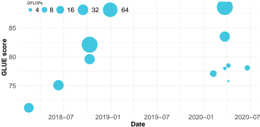<details> <summary>Image 15 Details</summary>  ### Visual Description ## Bubble Chart: GLUE Score vs. Date and GFLOPS ### Overview The image is a bubble chart showing the relationship between GLUE score, date, and GFLOPS. The x-axis represents the date, the y-axis represents the GLUE score, and the size of the bubbles represents the GFLOPS. The chart displays data points from 2018-07 to 2020-07. ### Components/Axes * **X-axis:** Date, with markers at 2018-07, 2019-01, 2019-07, 2020-01, and 2020-07. * **Y-axis:** GLUE score, ranging from approximately 71 to 87, with markers at 75, 80, and 85. * **Bubble Size:** Represents GFLOPS, with a legend at the top indicating the size of the bubbles for 4, 8, 16, 32, and 64 GFLOPS. The bubbles are all the same color, a light blue. ### Detailed Analysis * **2018-07:** One data point with a GLUE score of approximately 72 and a GFLOPS of 4. * **2018-07:** One data point with a GLUE score of approximately 75 and a GFLOPS of 8. * **2019-01:** Two data points. One with a GLUE score of approximately 79 and a GFLOPS of 32. The other with a GLUE score of approximately 82 and a GFLOPS of 32. * **2020-01:** Multiple data points. One with a GLUE score of approximately 77 and a GFLOPS of 16. One with a GLUE score of approximately 77 and a GFLOPS of 8. One with a GLUE score of approximately 76 and a GFLOPS of 8. One with a GLUE score of approximately 83 and a GFLOPS of 32. One with a GLUE score of approximately 87 and a GFLOPS of 64. * **2020-07:** Two data points. One with a GLUE score of approximately 78 and a GFLOPS of 8. One with a GLUE score of approximately 78 and a GFLOPS of 16. ### Key Observations * The GLUE score generally increases with GFLOPS. * The GLUE score generally increases over time. * There is a cluster of data points in 2020-01, indicating a period of significant experimentation or data collection. ### Interpretation The bubble chart suggests a positive correlation between GFLOPS and GLUE score, indicating that higher computational power generally leads to better performance on the GLUE benchmark. The trend over time also suggests improvements in GLUE scores, potentially due to advancements in models, training techniques, or hardware. The cluster of data points in 2020-01 could indicate a period of rapid development or experimentation, where different configurations were tested to optimize performance. The data shows that the highest GLUE score was achieved in 2020-01 with 64 GFLOPS. </details> ## FLOPS estimation for CV models ## EfficientNet-Based Models FLOPs Estimation There are many EfficientNet variations, mostly using different input resolution or scaling. For these modifications, FLOPs are not always reported. In this work, we estimate them following the relation presented in Equation 3 $$F L O P s \, \infty \, d + w ^ { 2 } + r ^ { 2 } \quad ( 3 )$$ for the following models: - NoisyStudent-L2 : Having the scale factors of the networks (Table 5) we estimate NoisyStudent-L2 FLOPs as shown in Equation 4 9 https://blogs.nvidia.com/blog/2020/05/14/tensorfloat-32-precision-format/ ## NLP data Many times researchers report GLUE score without the punctuation on the WNLI task, because this task is problematic. We have marked which scores are reported without this task. Since there are 9 tasks in total, we consider that excluding one of them is not problematic for our analysis. We did not find inference GFLOPs for the model Bert-Large, but we have ELECTRA-Large GFLOPs and this is actually the same model but following a different training strategy. In this Table 5: EfficientNet models architecture specifications obtained from [Xie et al., 2020]. | Model | w | d | Test Resolution | |-----------------|-----|-----|-------------------| | EfficientNet-B7 | 2 | 3.1 | 600 × 600 | | EfficientNet-L2 | 4.3 | 5.3 | 800 × 800 | $$\begin{array} { r l r } & { N o i s y S t u d e n - L 2 F L O P s = } \\ & { = E f f i c i e n T e n t - B 7 F L O P s \cdot d _ { \sigma } \cdot w _ { \sigma } ^ { 2 } \cdot r _ { \sigma } ^ { 2 } } \end{array}$$ where d σ , w σ and r σ are the scaled factors for, respectively, the network depth, width and input resolutions. By using the values from Table 5, d σ = 5 . 3 / 3 . 1 = 1 . 7097 , w σ = 4 . 3 / 2 = 2 . 15 and r σ = 800 / 600 = 1 . 3334 . Knowing that the GFLOPS for EfficientNetB7 are 74, substituting in 4, we obtain the estimation of 74 GFLOPs · 1 . 7097 · 2 . 15 2 · 1 . 3334 2 ≈ 1040 GFLOPS for NoisyStudent-L2. - Meta Pseudo Labels L2 : We use the estimation of NoisyStudent-L2 FLOPs for Meta Pseudo Labels L2, because it is the same model and only changes the training strategy. - FixEfficientNet-L2 : In FixEfficientNet-L2 they use a resolution of 600 × 600 for testing, so the estimation is the same as for NoisyStudent-L2 but without taking into account the resolution scaling ( r σ ). Then, the estimated GFLOPS are 74 GFLOPs · 1 . 7097 · 2 . 15 2 ≈ 585 GFLOPS. - FixEfficientNet-B7 : This model is the same as EfficientNet-B7 but using a slightly different resolution ( 632 × 632 ). Therefore, r σ = 632 / 600 = 1 . 0534 and, thus we estimate 74 GFLOPs · 1 . 0534 2 ≈ 82 GFLOPs. - FixEfficientNet-B0 : This model is the same as EfficientNet-B0 but using a higher resolution ( 320 × 320 ). Therefore, r σ = 320 / 224 = 1 . 4286 and, thus we estimate 0 . 78 GFLOPs · 1 . 4286 2 ≈ 1 . 6 GFLOPs. ## ViT-G/14 FLOPs Estimation In the paper [Zhai et al., 2021] introducing the model, although authors provide the GFLOPs for 224 × 224 and 384 × 384 resolutions (see Table 6), they also also use 518 × 518 resolution for ViT-G finetuning, so we assume they use the same resolution for testing too. ViT-G/14 is a vision transformer model, so the scale relation presented in 3 do not apply for this kind of models. However, knowing the GFLOPs for 224 × 224 and 384 × 384 , we may calculate how GFLOPs scale with resolution (given that r 2 σ = (384 / 224) 2 = 2 . 9388 ). In this regard, we calculate the GFLOPs ratio as 2859 . 9 / 965 . 3 = 2 . 9627 and we observe that GFLOPs scale quadratically with respect to resolution. Note, in this paper they report 'real' FLOPs and not multiply-add operations. Therefore, we recalculate r σ = 518 / 384 = 1 . 3490 and multiply the GFLOPs for 384 × 384 resolution by this scale factor estimating 2859 . 9 GFLOPs · 1 . 3490 2 ≈ 5270 GFLOPs for the ViT-G/14 model. Table 6: ViT-G/14 GFLOPs from. | Model | GFLOPS | GFLOPS | |----------|-----------|-----------| | Model | 224 × 224 | 384 × 384 | | ViT-G/14 | 965.3 | 2859.9 | sense, we use take ELECTRA-Large GFLOPs as BERT-Large GFLOPs. For ELMo we take GLUE 'dev-set' score because we do not found the score on the test set (we assume this score should be close to the test set). Values shown in Table 7. Table 7: NLP models data set. If there is a citation next to the GFLOPs value means that GFLOPs and Input Tokens values are extracted from that source, otherwise the values are from the paper (cited in the 'Model' column). The symbol ♠ means that GLUE score was calculated without punctuation on the WNLI task; the symbol ∗ means that we estimated the value and ♣ means that GLUE score is for GLUE dev set instead of test set. 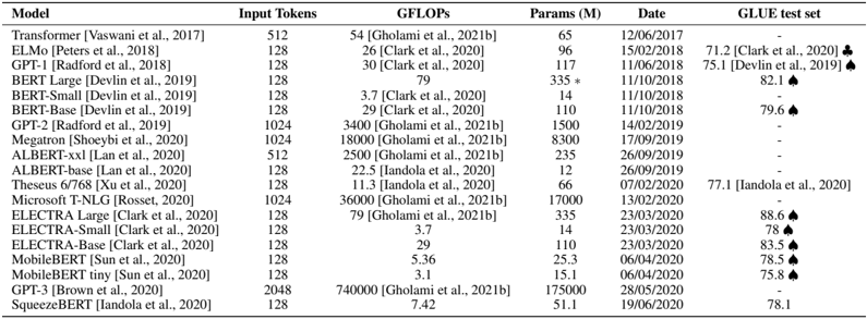<details> <summary>Image 16 Details</summary>  ### Visual Description ## Data Table: Model Performance Metrics ### Overview The image presents a data table comparing the performance metrics of various language models. The table includes information on the model name, input tokens, GFLOPs, number of parameters, date, and GLUE test set performance. ### Components/Axes The table has the following columns: * **Model**: Name of the language model, along with the publication reference. * **Input Tokens**: Number of input tokens used by the model. * **GFLOPs**: Giga Floating Point Operations per second, a measure of computational cost. * **Params (M)**: Number of parameters in millions. * **Date**: Date of the model's publication or evaluation. * **GLUE test set**: Performance on the GLUE (General Language Understanding Evaluation) benchmark. ### Detailed Analysis or ### Content Details Here's a breakdown of the data for each model: * **Transformer [Vaswani et al., 2017]**: Input Tokens: 512, GFLOPs: 54 [Gholami et al., 2021b], Params (M): 65, Date: 12/06/2017, GLUE test set: - * **ELMo [Peters et al., 2018]**: Input Tokens: 128, GFLOPs: 26 [Clark et al., 2020], Params (M): 96, Date: 15/02/2018, GLUE test set: 71.2 [Clark et al., 2020] * **GPT-1 [Radford et al., 2018]**: Input Tokens: 128, GFLOPs: 30 [Clark et al., 2020], Params (M): 117, Date: 11/06/2018, GLUE test set: 75.1 [Devlin et al., 2019] * **BERT Large [Devlin et al., 2019]**: Input Tokens: 128, GFLOPs: 79, Params (M): 335 *, Date: 11/10/2018, GLUE test set: 82.1 * **BERT-Small [Devlin et al., 2019]**: Input Tokens: 128, GFLOPs: 3.7 [Clark et al., 2020], Params (M): 14, Date: 11/10/2018, GLUE test set: - * **BERT-Base [Devlin et al., 2019]**: Input Tokens: 128, GFLOPs: 29 [Clark et al., 2020], Params (M): 110, Date: 11/10/2018, GLUE test set: 79.6 * **GPT-2 [Radford et al., 2019]**: Input Tokens: 1024, GFLOPs: 3400 [Gholami et al., 2021b], Params (M): 1500, Date: 14/02/2019, GLUE test set: - * **Megatron [Shoeybi et al., 2020]**: Input Tokens: 1024, GFLOPs: 18000 [Gholami et al., 2021b], Params (M): 8300, Date: 17/09/2019, GLUE test set: - * **ALBERT-xxl [Lan et al., 2020]**: Input Tokens: 512, GFLOPs: 2500 [Gholami et al., 2021b], Params (M): 235, Date: 26/09/2019, GLUE test set: - * **ALBERT-base [Lan et al., 2020]**: Input Tokens: 128, GFLOPs: 22.5 [Iandola et al., 2020], Params (M): 12, Date: 26/09/2019, GLUE test set: - * **Theseus 6/768 [Xu et al., 2020]**: Input Tokens: 128, GFLOPs: 11.3 [Iandola et al., 2020], Params (M): 66, Date: 07/02/2020, GLUE test set: 77.1 [Iandola et al., 2020] * **Microsoft T-NLG [Rosset, 2020]**: Input Tokens: 1024, GFLOPs: 36000 [Gholami et al., 2021b], Params (M): 17000, Date: 13/02/2020, GLUE test set: - * **ELECTRA Large [Clark et al., 2020]**: Input Tokens: 128, GFLOPs: 79 [Gholami et al., 2021b], Params (M): 335, Date: 23/03/2020, GLUE test set: 88.6 * **ELECTRA-Small [Clark et al., 2020]**: Input Tokens: 128, GFLOPs: 3.7, Params (M): 14, Date: 23/03/2020, GLUE test set: 78 * **ELECTRA-Base [Clark et al., 2020]**: Input Tokens: 128, GFLOPs: 29, Params (M): 110, Date: 23/03/2020, GLUE test set: 83.5 * **MobileBERT [Sun et al., 2020]**: Input Tokens: 128, GFLOPs: 5.36, Params (M): 25.3, Date: 06/04/2020, GLUE test set: 78.5 * **MobileBERT tiny [Sun et al., 2020]**: Input Tokens: 128, GFLOPs: 3.1, Params (M): 15.1, Date: 06/04/2020, GLUE test set: 75.8 * **GPT-3 [Brown et al., 2020]**: Input Tokens: 2048, GFLOPs: 740000 [Gholami et al., 2021b], Params (M): 175000, Date: 28/05/2020, GLUE test set: - * **SqueezeBERT [Iandola et al., 2020]**: Input Tokens: 128, GFLOPs: 7.42, Params (M): 51.1, Date: 19/06/2020, GLUE test set: 78.1 ### Key Observations * GPT-3 has significantly higher GFLOPs and parameters compared to other models. * The GLUE test set performance varies across different models. * The table includes models published between 2017 and 2020. ### Interpretation The data table provides a snapshot of the landscape of language models, highlighting the trade-offs between model size (parameters), computational cost (GFLOPs), and performance on a specific benchmark (GLUE). The evolution of models is evident, with newer models like GPT-3 having substantially larger sizes and computational requirements. The GLUE test set results offer a way to compare the models' general language understanding capabilities, although it's important to note that this is just one metric and may not fully capture the nuances of each model's performance. The absence of GLUE test set scores for some models suggests that these models may not have been evaluated on this particular benchmark or that the results were not available at the time of publication. The asterisk next to the parameter count for BERT Large suggests a possible annotation or caveat regarding that specific value. </details> | Model | Input Tokens | GFLOPs | Params (M) | Date | GLUE test set | |------------------------------------|----------------|--------------------------------|--------------|------------|------------------------------| | Transformer [Vaswani et al., 2017] | 512 | 54 [Gholami et al., 2021b] | 65 | 12/06/2017 | - | | ELMo [Peters et al., 2018] | 128 | 26 [Clark et al., 2020] | 96 | 15/02/2018 | 71.2 [Clark et al., 2020] ♣ | | GPT-1 [Radford et al., 2018] | 128 | 30 [Clark et al., 2020] | 117 | 11/06/2018 | 75.1 [Devlin et al., 2019] ♠ | | BERT Large [Devlin et al., 2019] | 128 | 79 | 335 ∗ | 11/10/2018 | 82.1 ♠ | | BERT-Small [Devlin et al., 2019] | 128 | 3.7 [Clark et al., 2020] | 14 | 11/10/2018 | - | | BERT-Base [Devlin et al., 2019] | 128 | 29 [Clark et al., 2020] | 110 | 11/10/2018 | 79.6 ♠ | | GPT-2 [Radford et al., 2019] | 1024 | 3400 [Gholami et al., 2021b] | 1500 | 14/02/2019 | - | | Megatron [Shoeybi et al., 2020] | 1024 | 18000 [Gholami et al., 2021b] | 8300 | 17/09/2019 | - | | ALBERT-xxl [Lan et al., 2020] | 512 | 2500 [Gholami et al., 2021b] | 235 | 26/09/2019 | - | | ALBERT-base [Lan et al., 2020] | 128 | 22.5 [Iandola et al., 2020] | 12 | 26/09/2019 | - | | Theseus 6/768 [Xu et al., 2020] | 128 | 11.3 [Iandola et al., 2020] | 66 | 07/02/2020 | 77.1 [Iandola et al., 2020] | | Microsoft T-NLG [Rosset, 2020] | 1024 | 36000 [Gholami et al., 2021b] | 17000 | 13/02/2020 | - | | ELECTRA Large [Clark et al., 2020] | 128 | 79 [Gholami et al., 2021b] | 335 | 23/03/2020 | 88.6 ♠ | | ELECTRA-Small [Clark et al., 2020] | 128 | 3.7 | 14 | 23/03/2020 | 78 ♠ | | ELECTRA-Base [Clark et al., 2020] | 128 | 29 | 110 | 23/03/2020 | 83.5 ♠ | | MobileBERT [Sun et al., 2020] | 128 | 5.36 | 25.3 | 06/04/2020 | 78.5 ♠ | | MobileBERT tiny [Sun et al., 2020] | 128 | 3.1 | 15.1 | 06/04/2020 | 75.8 ♠ | | GPT-3 [Brown et al., 2020] | 2048 | 740000 [Gholami et al., 2021b] | 175000 | 28/05/2020 | - | | SqueezeBERT [Iandola et al., 2020] | 128 | 7.42 | 51.1 | 19/06/2020 | 78.1 | ## GPU consumption data Tables 8 and 9 show further technical details regarding, respectively, the GPU's theoretical characteristics (compiled from the manufacturer's specification sheet and reference manuals), and their throughput and power consumption 'adapted', if necessary, to the specifics of CV or NLP tasks. Table 8: Nvidia GPUs theoretical data recopilation. 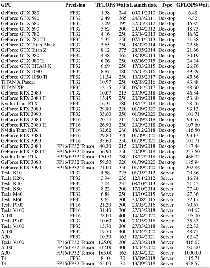<details> <summary>Image 17 Details</summary>  ### Visual Description ## Data Table: GPU Performance Metrics ### Overview The image presents a data table comparing the performance of various GPUs (Graphics Processing Units) based on several metrics. The table includes GPU name, precision, TFLOPS (Tera Floating Point Operations Per Second), Watts, launch date, type (Desktop or Server), and GFLOPS/Watt (Giga Floating Point Operations Per Second per Watt). ### Components/Axes The table has the following columns: * **GPU:** Name of the GPU (e.g., GeForce GTX 580, Tesla K10, A100). * **Precision:** Floating-point precision supported by the GPU (e.g., FP32, FP16, FP16/FP32 Tensor). * **TFLOPS:** Theoretical compute performance in Tera Floating Point Operations Per Second. * **Watts:** Power consumption of the GPU in Watts. * **Launch date:** Date when the GPU was launched (MM/DD/YYYY). * **Type:** Indicates whether the GPU is designed for Desktops or Servers. * **GFLOPS/Watt:** Performance per Watt, calculated as GFLOPS divided by Watts. ### Detailed Analysis or ### Content Details Here's a breakdown of the data, including specific values and trends: * **GeForce GTX Series:** * The GeForce GTX series includes models from GTX 580 to GTX 1080 Ti. * TFLOPS ranges from 1.58 (GTX 580) to 11.34 (GTX 1080 Ti). * Watts range from 165 (GTX 980) to 375 (GTX Titan Z). * GFLOPS/Watt ranges from 6.48 (GTX 580) to 49.29 (GTX 1080). * **TITAN Series:** * Includes TITAN X Pascal and TITAN XP. * TFLOPS are 10.97 and 12.15, respectively. * Both consume 250 Watts. * GFLOPS/Watt are 43.88 and 48.60, respectively. * **GeForce RTX Series (FP32):** * Includes RTX 2080, RTX 2080 Ti, RTX 3080, and RTX 3090. * TFLOPS ranges from 10.07 (RTX 2080) to 35.60 (RTX 3090). * Watts range from 215 (RTX 2080) to 350 (RTX 3090). * GFLOPS/Watt ranges from 46.84 (RTX 2080) to 101.71 (RTX 3090). * **GeForce RTX Series (FP16):** * Includes RTX 2080, RTX 2080 Ti, RTX 3080, and RTX 3090. * TFLOPS ranges from 20.14 (RTX 2080) to 35.60 (RTX 3090). * Watts range from 215 (RTX 2080) to 350 (RTX 3090). * GFLOPS/Watt ranges from 93.13 (RTX 3080) to 116.50 (Nvidia Titan RTX). * **GeForce RTX Series (FP16/FP32 Tensor):** * Includes RTX 2080, RTX 2080 Ti, RTX 3080, and RTX 3090. * TFLOPS ranges from 40.30 (RTX 2080) to 71.00 (RTX 3090). * Watts range from 215 (RTX 2080) to 350 (RTX 3090). * GFLOPS/Watt ranges from 185.94 (RTX 3080) to 466.07 (Nvidia Titan RTX). * **Nvidia Titan RTX:** * Available in FP32, FP16, and FP16/FP32 Tensor precisions. * TFLOPS are 16.31 (FP32), 32.62 (FP16), and 130.50 (FP16/FP32 Tensor). * Watts are 280 for all precisions. * GFLOPS/Watt are 58.26 (FP32), 116.50 (FP16), and 466.07 (FP16/FP32 Tensor). * **Tesla Series:** * Includes models from K10 to V100. * TFLOPS ranges from 3.94 (K20x) to 31.40 (V100). * Watts range from 225 (K10) to 300 (multiple models). * GFLOPS/Watt ranges from 16.74 (K20x) to 104.67 (V100). * **A100 Series:** * Available in FP16, FP32, and FP16/FP32 Tensor precisions. * TFLOPS are 78.00 (FP16), 19.50 (FP32), and 312.00 (FP16/FP32 Tensor). * Watts are 400 for all precisions. * GFLOPS/Watt are 48.75 (FP32), 195.00 (FP16), and 780.00 (FP16/FP32 Tensor). * **A30 Series:** * Available in FP32 and FP16/FP32 Tensor precisions. * TFLOPS are 10.30 (FP32) and 165.00 (FP16/FP32 Tensor). * Watts are 165 for all precisions. * GFLOPS/Watt are 62.42 (FP32) and 1000.00 (FP16/FP32 Tensor). * **T4 Series:** * Available in FP32 and FP16/FP32 Tensor precisions. * TFLOPS are 8.10 (FP32) and 65.00 (FP16/FP32 Tensor). * Watts are 70 for all precisions. * GFLOPS/Watt are 115.71 (FP32) and 928.57 (FP16/FP32 Tensor). ### Key Observations * GPUs with FP16/FP32 Tensor precision generally have higher TFLOPS and GFLOPS/Watt compared to FP32 or FP16 alone. * Server GPUs (Tesla, A100, A30, T4) tend to have higher GFLOPS/Watt than Desktop GPUs (GeForce GTX, RTX, TITAN). * Newer GPUs generally offer higher TFLOPS and GFLOPS/Watt compared to older models. * Power consumption (Watts) varies significantly across different GPUs. ### Interpretation The data demonstrates the evolution of GPU technology, showcasing improvements in performance (TFLOPS) and energy efficiency (GFLOPS/Watt) over time. The shift towards FP16 and Tensor cores indicates a focus on machine learning and AI workloads, where lower precision can be used to accelerate computations. The distinction between Desktop and Server GPUs highlights the different design priorities, with Server GPUs prioritizing performance per watt for data center environments. The table allows for a direct comparison of different GPUs based on key performance metrics, aiding in the selection of the most suitable GPU for a given application. </details> | GPU | Precision | TFLOPSWatts | | Launch date | Type | GFLOPS/Watt | |-------------------------|------------------|---------------|---------|---------------|---------|---------------| | GeForce GTX 580 | FP32 | 1.58 | 244 | 09/11/2010 | Desktop | 6.48 | | GeForce GTX 590 | FP32 | 2.49 | 365 | 24/03/2011 | Desktop | 6.82 | | GeForce GTX 680 | FP32 | 3.09 | 195 | 22/03/2012 | Desktop | 15.85 | | GeForce GTX 690 | FP32 | 5.62 | 300 | 29/04/2012 | Desktop | 18.73 | | GeForce GTX 780 | FP32 | 4.16 | 250 | 23/04/2013 | Desktop | 16.62 | | GeForce GTX 780 TI | FP32 | 5.35 | 250 | 07/11/2013 | Desktop | 21.38 | | GeForce GTX Titan Black | FP32 | 5.65 | 250 | 18/02/2014 | Desktop | 22.58 | | GeForce GTX Titan Z | FP32 | 8.12 | 375 | 28/05/2014 | Desktop | 21.66 | | GeForce GTX 980 | FP32 | 4.98 | 165 | 18/09/2014 | Desktop | 30.19 | | GeForce GTX 980 Ti | FP32 | 6.06 | 250 | 02/06/2015 | Desktop | 24.24 | | GeForce GTX TITAN X | FP32 | 6.69 | 250 | 17/03/2015 | Desktop | 26.76 | | GeForce GTX 1080 | FP32 | 8.87 | 180 | 26/05/2016 | Desktop | 49.29 | | GeForce GTX 1080 Ti | FP32 | 11.34 | 250 | 10/03/2017 | Desktop | 45.36 | | TITAN X Pascal | FP32 | 10.97 | 250 | 02/08/2016 | Desktop | 43.88 | | TITAN XP | FP32 | 12.15 | 250 | 06/04/2017 | Desktop | 48.6 | | GeForce RTX 2080 | FP32 | 10.07 | 215 | 20/09/2018 | Desktop | 46.84 | | GeForce RTX 2080 Ti | FP32 | 13.45 | 250 | 20/09/2018 | Desktop | 53.8 | | Nvidia Titan RTX | FP32 | 16.31 | 280 | 18/12/2018 | Desktop | 58.26 | | GeForce RTX 3080 | FP32 | 29.8 | 320 | 01/09/2020 | Desktop | 93.13 | | GeForce RTX 3090 | FP32 | 35.6 | 350 | 01/09/2020 | Desktop | 101.71 | | GeForce RTX 2080 | FP16 | 20.14 | 215 | 20/09/2018 | Desktop | 93.67 | | GeForce RTX 2080 Ti | FP16 | 26.9 | 250 | 20/09/2018 | Desktop | 107.6 | | Nvidia Titan RTX | FP16 | 32.62 | 280 | 18/12/2018 | Desktop | 116.5 | | GeForce RTX 3080 | FP16 | 29.8 | 320 | 01/09/2020 | Desktop | 93.13 | | GeForce RTX 3090 | FP16 | 35.6 | 350 | 01/09/2020 | Desktop | 101.71 | | GeForce RTX 2080 | FP16/FP32 Tensor | 40.3 | 215 | 20/09/2018 | Desktop | 187.44 | | GeForce RTX 2080 Ti | FP16/FP32 Tensor | 56.9 | 250 | 20/09/2018 | Desktop | 227.6 | | Nvidia Titan RTX | FP16/FP32 Tensor | 130.5 | 280 | 18/12/2018 | Desktop | 466.07 | | GeForce RTX 3080 | FP16/FP32 Tensor | 59.5 | 320 | 01/09/2020 | Desktop | 185.94 | | GeForce RTX 3090 | FP16/FP32 Tensor | 71 | 350 | 01/09/2020 | Desktop | 202.86 | | Tesla K10 | FP32 | 4.58 | 225 | 01/05/2012 | Server | 20.36 | | Tesla K20x | FP32 | 3.94 | 235 | 12/11/2012 | Server | 16.74 | | Tesla K40 | FP32 | 5.04 | 235 | 08/10/2013 | Server | 21.45 | | Tesla K80 | FP32 | 8.22 | 300 | 17/10/2014 | Server | 27.4 | | Tesla M40 | FP32 | 6.84 | 250 | 10/10/2015 | Server | 27.36 | | Tesla M60 | FP32 | 9.65 | 300 | 30/08/2015 | Server | 32.17 | | Tesla P100 | FP16 | 21.2 | 300 | 20/05/2016 | Server | 70.67 | | Tesla V100 | FP16 | 31.4 | 300 | 27/03/2018 | Server | 104.67 | | A100 | FP16 | 78 | 400 | 14/04/2020 | Server | 195 | | Tesla P100 | FP32 | 10.6 | 300 | 20/05/2016 | Server | 35.33 | | Tesla V100 | FP32 | 15.7 | 300 | 27/03/2018 | Server | 52.33 | | A100 | FP32 | 19.5 | 400 | 14/04/2020 | Server | 48.75 | | A30 | FP32 | 10.3 | 165 | 12/04/2021 | Server | 62.42 | | Tesla V100 | FP16/FP32 Tensor | 125 | 300 | 27/03/2018 | Server | 416.67 | | A100 | FP16/FP32 Tensor | 312 | | 14/04/2020 | Server | 780 | | A30 | FP16/FP32 Tensor | 165 | 400 165 | 12/04/2021 | Server | 1000 | | T4 | FP32 | 8.1 | 70 | 13/09/2018 | Server | 115.71 | | T4 | FP16/FP32 Tensor | 65 | 70 | 13/09/2018 | Server | 928.57 | Table 9: GPUs throughput and power consumption data compilation. | Adapted | GPU | Precision | TFLOPSWatts | | Launch date | Type | GFLOPS/Watt | |-----------|-------------------------|-------------|---------------|-----|---------------|---------|---------------| | | GeForce GTX 580 | FP32 | 1.58 | 244 | 09/11/2010 | Desktop | 6.48 | | | GeForce GTX 590 | FP32 | 2.49 | 365 | 24/03/2011 | Desktop | 6.82 | | | GeForce GTX 680 | FP32 | 3.09 | 195 | 22/03/2012 | Desktop | 15.85 | | | GeForce GTX 690 | FP32 | 5.62 | 300 | 29/04/2012 | Desktop | 18.73 | | | Tesla K10 | FP32 | 4.58 | 225 | 01/05/2012 | Server | 20.36 | | | Tesla K20x | FP32 | 3.94 | 235 | 12/11/2012 | Server | 16.77 | | | GeForce GTX 780 | FP32 | 4.16 | 250 | 23/04/2013 | Desktop | 16.64 | | | Tesla K40 | FP32 | 5.04 | 235 | 08/10/2013 | Server | 21.45 | | | GeForce GTX 780 TI | FP32 | 5.35 | 250 | 07/11/2013 | Desktop | 21.4 | | | GeForce GTX Titan Black | FP32 | 5.65 | 250 | 18/02/2014 | Desktop | 22.6 | | | GeForce GTX Titan Z | FP32 | 8.12 | 375 | 28/05/2014 | Desktop | 21.65 | | | GeForce GTX 980 | FP32 | 4.98 | 165 | 18/09/2014 | Desktop | 30.18 | | | Tesla K80 | FP32 | 8.22 | 300 | 17/10/2014 | Server | 27.4 | | No | GeForce GTX TITAN X | FP32 | 6.69 | 250 | 17/03/2015 | Desktop | 26.76 | | No | GeForce GTX 980 Ti | FP32 | 6.06 | 250 | 02/06/2015 | Desktop | 24.24 | | No | Tesla M60 | FP32 | 9.65 | 300 | 30/08/2015 | Server | 32.17 | | No | Tesla M40 | FP32 | 6.84 | 250 | 10/10/2015 | Server | 27.36 | | No | GeForce GTX 1080 | FP32 | 8.87 | 180 | 26/05/2016 | Desktop | 49.28 | | No | TITAN X Pascal | FP32 | 10.97 | 250 | 02/08/2016 | Desktop | 43.88 | | No | GeForce GTX 1080 Ti | FP32 | 11.34 | 250 | 10/03/2017 | Desktop | 45.36 | | No | TITAN XP | FP32 | 12.15 | 250 | 06/04/2017 | Desktop | 48.6 | | No | Tesla V100 | FP32 | 15.7 | 300 | 27/03/2018 | Server | 52.33 | | No | Tesla T4 | FP32 | 8.1 | 70 | 13/09/2018 | Server | 115.71 | | No | GeForce RTX 2080 | FP32 | 10.07 | 215 | 20/09/2018 | Desktop | 46.84 | | No | GeForce RTX 2080 Ti | FP32 | 13.45 | 250 | 20/09/2018 | Desktop | 53.8 | | No | Nvidia Titan RTX | FP32 | 16.31 | 280 | 18/12/2018 | Desktop | 58.25 | | No | GeForce RTX 3080 | FP32 | 29.8 | 320 | 01/09/2020 | Desktop | 93.13 | | No | GeForce RTX 3090 | FP32 | 35.6 | 350 | 01/09/2020 | Desktop | 101.71 | | For CNN | Tesla V100 | Mixed | 35.71 | 300 | 27/03/2018 | Server | 119.03 | | For CNN | Tesla T4 | Mixed | 21.85 | 70 | 13/09/2018 | Server | 312.15 | | For CNN | A100 | TF32 | 27.41 | 400 | 14/04/2020 | Server | 68.52 | | For CNN | A100 | Mixed | 52.35 | 400 | 14/04/2020 | Server | 130.88 | | For NLP | Tesla V100 | Mixed | 41.44 | 300 | 27/03/2018 | Server | 138.13 | | For NLP | Tesla T4 | Mixed | 25.58 | 70 | 13/09/2018 | Server | 365.46 | | For NLP | A100 | TF32 | 55.85 | 400 | 14/04/2020 | Server | 139.64 | | For NLP | A100 | Mixed | 73.29 | 400 | 14/04/2020 | Server | 183.23 |