## All-optical scalable spatial coherent Ising machine
Marcello Calvanese Strinati, 1, ∗ Davide Pierangeli, 1, 2 and Claudio Conti 1, 2, 3
1 Physics Department, Sapienza University of Rome, 00185 Rome, Italy
2 Institute for Complex Systems, National Research Council (ISC-CNR), 00185 Rome, Italy
3 Centro Ricerche Enrico Fermi (CREF), Via Panisperna 89a, 00184 Rome, Italy
(Dated: November 15, 2021)
Networks of optical oscillators simulating coupled Ising spins have been recently proposed as a heuristic platform to solve hard optimization problems. These networks, called coherent Ising machines (CIMs), exploit the fact that the collective nonlinear dynamics of coupled oscillators can drive the system close to the global minimum of the classical Ising Hamiltonian, encoded in the coupling matrix of the network. To date, realizations of large-scale CIMs have been demonstrated using hybrid optical-electronic setups, where optical oscillators simulating different spins are subject to electronic feedback mechanisms emulating their mutual interaction. While the optical evolution ensures an ultrafast computation, the electronic coupling represents a bottleneck that causes the computational time to severely depend on the system size. Here, we propose an all-optical scalable CIM with fully-programmable coupling. Our setup consists of an optical parametric amplifier with a spatial light modulator (SLM) within the parametric cavity. The spin variables are encoded in the binary phases of the optical wavefront of the signal beam at different spatial points, defined by the pixels of the SLM. We first discuss how different coupling topologies can be achieved by different configurations of the SLM, and then benchmark our setup with a numerical simulation that mimics the dynamics of the proposed machine. In our proposal, both the spin dynamics and the coupling are fully performed in parallel, paving the way towards the realization of size-independent ultrafast optical hardware for large-scale computation purposes.
## I. INTRODUCTION
Solving large-scale optimization problems is extremely useful to several different fields of modern science, with applications ranging from biology to finance and social science [1-5]. These problems often belong to the nondeterministic polynomial (NP-hard) computational complexity class [6]: Finding the optimal solution requires computational resources that scale exponentially with the size of the system, making these problems intractable using conventional computer architectures. A tremendous amount of interest has been recently attracted by the development of unconventional computational methods (heuristic solvers) to solve probabilistically, but efficiently, large-scale optimization problems. A key observation behind these heuristic methods is that optimization problems can be mapped onto specific classical Ising models efficiently [7], i.e., in a polynomial (P) time. Solving the specific optimization problem then translates into the NP-hard problem of finding the ground state (GS) of the corresponding Ising Hamiltonian [8].
In recent years, several physical systems have been demonstrated to evolve according to the classical Ising Hamiltonian, therefore providing valuable ad hoc platforms to solve the Ising model for large-scale optimization purposes. Remarkable examples include two-component Bose-Einstein condensates [9, 10], superconducting circuits [11], trapped ions [12, 13], digital computers [14-17], electrical oscillators [18], optoelectronical oscillators [19], polariton condensates [20-22], laser networks [23, 24],
∗ marcello.calvanesestrinati@gmail.com
and coupled optical parametric oscillators (OPOs) [2538], which are the focus of this work. These networks, called coherent Ising machines (CIMs) exploit the fact that, when driven above the oscillation threshold, a second-order phase transition takes place [39, 40]: In the long-time limit, the phase of each OPO takes values 0 or π with respect to the reference phase enforced by the pump. Because of the bistable nature of its phase, an OPO is suitable to simulate a classical Ising spin, and systems of coupled OPOs in proper conditions can simulate the dynamics of coupled Ising spins [29, 41, 42].
Nowadays, major issues in realizing CIMs for realistic optimization problems involve, on one hand, the physical conditions (e.g., temperature) in which the machine has to operate, and on the other hand, the scalability and the connectivity that these systems can implement. In this respect, photonic systems offer a versatile platform to realize large-scale CIMs with general connectivity, while working at room temperature and being constructed from off-the-shelf components. An implementation of an alloptical CIM with few spins using time-multiplexed OPOs has been reported in Refs. [26, 27], where different OPOs are different temporal pulses within a nonlinear cavity, and optical delay lines are used to couple different OPOs. This approach allows the realization of arbitrary coupling topology, but cannot be scaled up to a large number of spins. An all-optical CIM with a largenumber of spins was reported in Ref. [28], implementing the one-dimensional nearest-neighbor coupling via a Mach-Zehnder interferometer. While this other approach allows the implementation of several spins, the coupling topology was limited to nearest-neighbor coupling. Large-scale CIMs with arbitrary coupling topology
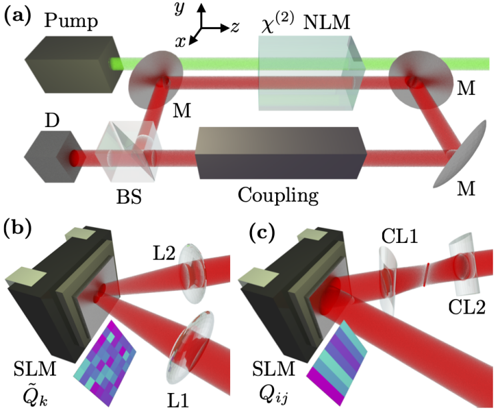
FIG. 1. (a) All-optical spatial CIM. The setup consists of the following: (i) χ (2) NLM pumped by a laser at wavelength λ p non-resonant with the cavity mirrors (M), which amplifies the signal at λ s = 2 λ p , (ii) Coupling mechanism, (iii) Extraction of the signal by a beam splitter (BS) with reflection and transmission coefficients R out and T out = √ 1 -R 2 out , respectively, and detection (D). The coupling is implemented using different configurations of the SLM depending on the implemented graph. (b) Circulant graphs: A first lens (L1) transforms the signal in Fourier space, the SLM multiplies the FT of the field by ˜ Q k , and a second lens (L2) transforms the modulated field back to real space. (c) General graphs, based on the vector-matrix multiplication scheme. The SLM works in real space, multiplying the incoming field by Q ij . The modulated signal is focused along the y -axis by a cylindrical lens (CL1), defocused, and rotated by 90 ◦ on the xy -plane by another cylindrical lens (CL2) with 45 ◦ rotated optical axis. The pixels in panels (b) and (c) depict the OPOs encoded on the xy -plane: An amplitude A j,τ is defined as a single pixel in panel (b) , whereas as a column of M y pixels in panel (c) .
<details>
<summary>Image 1 Details</summary>
### Visual Description
\n
## Diagram: Optical Setup for Nonlinear Microscopy
### Overview
The image depicts three schematic diagrams (a, b, and c) illustrating an optical setup likely used for nonlinear microscopy. The diagrams show the arrangement of optical components and the paths of laser beams (green and red) through the system. The diagrams are labeled with component names and include a coordinate system in diagram (a).
### Components/Axes
* **Diagram (a):**
* **Pump:** Laser source emitting a green beam.
* **χ<sup>(2)</sup> NLM:** Nonlinear Microscopy component.
* **M:** Mirrors (two instances).
* **BS:** Beam Splitter.
* **Coupling:** Coupling component.
* **D:** Detector.
* **Coordinate System:** x, y, and z axes are indicated in the top-right corner.
* **Diagram (b):**
* **SLM:** Spatial Light Modulator labeled as Q<sub>k</sub>. Displays a patterned image.
* **L1 & L2:** Lenses (two instances).
* **Diagram (c):**
* **SLM:** Spatial Light Modulator labeled as Q<sub>ij</sub>. Displays a patterned image.
* **CL1 & CL2:** Cylindrical Lenses (two instances).
### Detailed Analysis or Content Details
**Diagram (a):**
The green laser beam (Pump) enters from the left, passes through the χ<sup>(2)</sup> NLM component, and is reflected by two mirrors (M). A red beam originates from the detector (D), passes through a beam splitter (BS), and is coupled into the system. The coordinate system indicates that the x and y axes are horizontal, and the z axis is vertical.
**Diagram (b):**
A red beam enters from the left, passes through a Spatial Light Modulator (SLM) displaying a patterned image (blue and green squares). The beam is then focused by two lenses (L1 and L2).
**Diagram (c):**
A red beam enters from the left, passes through a Spatial Light Modulator (SLM) displaying a different patterned image (purple and blue gradients). The beam is then shaped by two cylindrical lenses (CL1 and CL2).
### Key Observations
* The diagrams show a progression of optical manipulation. Diagram (a) shows the basic setup, while diagrams (b) and (c) demonstrate how the beam can be shaped using SLMs and lenses.
* The SLMs in diagrams (b) and (c) display different patterns, suggesting that the system can generate various beam profiles.
* The use of cylindrical lenses in diagram (c) indicates that the beam is being shaped into an anisotropic form.
* The color coding (green for the pump laser, red for the signal/detection path) is consistent across all three diagrams.
### Interpretation
The diagrams illustrate a sophisticated optical setup for nonlinear microscopy. The system utilizes a pump laser (green) to induce nonlinear effects in a sample (within the χ<sup>(2)</sup> NLM component). The emitted signal (red) is then manipulated using a beam splitter, spatial light modulators, and lenses to control its spatial properties. The SLMs allow for precise control over the beam profile, enabling techniques such as structured illumination or multi-photon microscopy. The use of cylindrical lenses suggests the ability to create elongated or focused beams. The overall setup is designed to optimize signal collection and enhance imaging resolution. The diagrams suggest a system capable of generating complex beam shapes for advanced microscopy applications. The coordinate system in (a) provides a reference frame for understanding the spatial arrangement of the components. The different patterns on the SLMs in (b) and (c) indicate the system's flexibility in generating different beam profiles for various imaging modalities.
</details>
have been demonstrated using time-multiplexed OPOs in hybrid optical-electronic systems [32, 43], or optoelectronic oscillators [19]: Optical signals evolve in time subject to electronic measure and feedback mechanisms to emulate the spin-spin interaction. The optical nature of the setup ensures ultrafast computation. However, the presence of the electronic feedback inherently represents a 'bottleneck' that introduces an additional computational time that scales quadratically with the system size [44]. The realization of a scalable fully optical CIM without the hindrance of electronic components is thus highly desirable.
A step towards the realization of an all-optical scalable CIM has been recently made by exploiting spatial degrees of freedom of light [34, 45]. This approach relies on the usage of spatial light modulators (SLMs) to encode a spin variable σ j into the binary phase modulation of the optical field shining the j -th pixel of the SLM. An electronic feedback mechanism was also present. To date, a proposal of an all-optical scalable CIM implementing an arbitrary coupling topology is still missing. In this paper, we propose and theoretically validate an all-optical scalable spatial CIM with fully-programmable coupling. We first propose two different configurations of the SLM to realize two different classes of coupling, and then estimate the computational performance of our machine by means of a numerical simulation that closely mimics the temporal dynamics of coupled OPOs within a parametric cavity. We find that our proposed setup converges close to the minimum of the Ising Hamiltonian after a computational time that is orders of magnitude smaller compared to existing hybrid electro-optical setups.
This paper is organized as follows. In Sec. II, we discuss the scheme of our proposed setup. In Sec. III, we show our numerical results, and draw our conclusions in Sec. IV.
## II. SCHEME OF THE PROPOSED SETUP
The scheme of our machine is shown in Fig. 1 a . We consider an optical parametric cavity with a second-order nonlinear medium ( χ (2) NLM) of length L , shone by a pump laser (green beam) at wavelength λ p . We take z as the direction of propagation of light. The pump beam within the NLM parametrically amplifies degenerate pairs of signal and idler photons (red beam) at wavelength λ s = 2 λ p via spontaneous parametric down conversion. The spatial configuration of the signal wavefront on the xy -plane encodes the amplitudes { A j,τ } of the N OPO fields ( j = 1 , . . . , N ) at round trip number τ . These amplitudes are in general complex, i.e., the phase of the optical field on the xy -plane can take any value. However, the presence of the χ (2) NLM forces the optical phases to be either 0 or π with respect to the pump phase, making the amplitudes { A j,τ } effectively real, as detailed below.
Different configurations of the SLM with M x × M y pixels realize different couplings between different OPOs, as shown in panels (b) and (c) . In panel (b) , the SLM is placed at the focal plane of a first lens (L1). The discretization of the field in real (and thus momentum) space is enforced by the SLM: Different pixels define different OPO amplitudes, thereby defining N = M x × M y different OPOs. Since in commercial SLMs one typically has M x , M y ∼ 10 3 , this scheme allows to define N ∼ 10 6 OPOs. The SLM acts as a programmable matrix with a transmission function ˜ Q k , which multiplies at each round trip the Fourier transform (FT) of the incoming OPO amplitudes ˜ A k,τ = FT[ { A j,τ } ]. A second lens (L2) with same focal length as L1 transforms the modulated fields ˜ Q k ˜ A k,τ back to real space, yielding the inverse Fourier transform (IFT) of ˜ Q k ˜ A k,τ . By convolution theorem, the resulting field on each pixel after the FT-SLM-IFT sequence is A ′ j,τ = ∑ i Q i -j +1 A i,τ , where Q j is the IFT of ˜ Q k . The output takes the form of a cou-
pled field A ′ j,τ = ∑ i Q ij A i,τ , where the coupling matrix Q has entries Q ij ≡ Q i -j +1 . This matrix represent a rotationally invariant (or circulant) graph [46], where all nodes are equivalent. Notable examples are the nearestneighbor Ising chain and the M¨ obious ladder [26-28, 33].
While the coupling scheme in panel (b) gives the possibility to encode a large number of OPOs, granting a straightforward experimental implementation, it allows the implementation of a limited class of graph. To overcome this issue, we propose in panel (c) a different scheme for a general coupling matrix Q . This setup is based on the vector-matrix multiplication scheme [47]: The different OPOs are arranged on the xy -plane as different column vectors, such that the signal wavefront shines all M y pixels on a given column of the SLM with a uniform field. The SLM multiples in real space the vectorized signal with amplitude A j,τ by Q ij , such that the amplitude at the point ( i, j ) of the field after the SLM is Q ij A j,τ . Acylindrical lens (CL1) focuses the signal wavefront onto a single column along the y -axis, whose amplitude at point i is given by A ′ i,τ = ∑ j Q ij A j,τ . Propagation in free space defocuses the signal on the xy -plane, obtaining a vectorized signal arranged as a row matrix. Subsequent rotation by 90 ◦ of the field by a second cylindrical lens (CL2) recovers the structure of the signal as column vectors. Now, each column encodes the amplitude A ′ j,τ = ∑ i Q ij A i,τ , i.e., a coupled field with general Q ij . As such, this scheme implements any coupling matrix, but with the drawback that the OPOs need to be redundantly defined over M y pixels, limiting to N = M x the number of OPOs in the system.
We stress that the two coupling schemes presented here are fully optical and process all interactions in parallel, without need of electronic feedbacks. Since in our scheme the propagation of the OPOs within the cavity also occurs in parallel, our scheme realizes a size-independent large-scale spatial CIM [44], with critical advantages in terms of scaling and computational time compared to the existing hybrid optical-electronic devices.
In our setup, the binary nature of the phase of each OPO is enforced by the χ (2) NLM in Fig. 1 a . We inject into the NLM a pump field with spatially uniform wavefront that, at each pixel j on the xy -plane, mixes inside the NLM with the signal field. The subsequent dynamics along the z -axis, independently at each point, follows the second-order nonlinear wave equation [48] for the degenerate signal field { A j,τ } and pump { B j,τ } :
<!-- formula-not-decoded -->
where the star denotes complex conjugation. Here, κ = 2 πχ (2) /λ s n 2 , where χ (2) and n = n ( λ s ) are the nonlinear coefficient and the index of refraction of the NLM, respectively, and λ s = 2 π/k s . We assume perfect phase matching 2 k s = k p , where k s ( p ) is the wave vector of the signal (pump), which is achieved by tuning the temperature of the NLM to equalize the index of refraction for the signal and pump. To show phase-dependent amplification, we
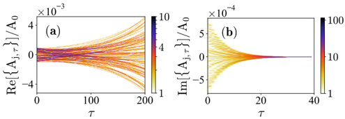
FIG. 2. Histogram of time evolution of the (a) real and (b) imaginary part of the N = 112 OPO amplitudes (in units of A 0 , see text), computed using Eq. (3), for short times. As evident, the cavity dynamics enhances the real part of the OPO amplitudes and suppresses their imaginary part.
<details>
<summary>Image 2 Details</summary>
### Visual Description
\n
## Chart: Real and Imaginary Parts of A<sub>i,τ</sub>/A<sub>0</sub>
### Overview
The image presents two charts, labeled (a) and (b), displaying the real and imaginary components of a normalized quantity, A<sub>i,τ</sub>/A<sub>0</sub>, as a function of τ. Both charts utilize a color scale to represent a third dimension of data. Chart (a) shows the real part (Re{A<sub>i,τ</sub>}) against τ, while chart (b) shows the imaginary part (Im{A<sub>i,τ</sub>}) against τ.
### Components/Axes
* **Chart (a):**
* X-axis: τ (ranging from approximately 0 to 200)
* Y-axis: Re{A<sub>i,τ</sub>}/A<sub>0</sub> (ranging from approximately -4 to 4, scaled by ×10<sup>-3</sup>)
* Colorbar: Represents values from 1 to 10, scaled by ×10<sup>-3</sup>.
* **Chart (b):**
* X-axis: τ (ranging from approximately 0 to 40)
* Y-axis: Im{A<sub>i,τ</sub>}/A<sub>0</sub> (ranging from approximately -5 to 5, scaled by ×10<sup>-4</sup>)
* Colorbar: Represents values from 1 to 100.
### Detailed Analysis or Content Details
**Chart (a):**
The chart displays a series of curves that initially diverge from the y-axis (Re{A<sub>i,τ</sub>}/A<sub>0</sub> = 0) at τ = 0. The curves generally slope downwards, becoming more spread out as τ increases. The color of the curves changes along their length, indicating variations in the value represented by the colorbar.
* At τ ≈ 0, the curves are predominantly yellow/orange (values around 1-4 on the colorbar).
* As τ increases to approximately 200, the curves transition to shades of purple/blue (values around 8-10 on the colorbar).
* The curves appear to converge slightly towards the end of the chart.
**Chart (b):**
This chart shows a similar pattern to chart (a), but with the imaginary component. The curves start at the y-axis (Im{A<sub>i,τ</sub>}/A<sub>0</sub> = 0) at τ = 0 and diverge.
* At τ ≈ 0, the curves are predominantly yellow/orange (values around 1-10 on the colorbar).
* As τ increases to approximately 40, the curves transition to shades of purple/red (values around 50-100 on the colorbar).
* The curves converge more rapidly in this chart than in chart (a).
### Key Observations
* Both charts exhibit a diverging pattern of curves, suggesting a complex relationship between A<sub>i,τ</sub> and τ.
* The colorbars indicate that the magnitude of A<sub>i,τ</sub>/A<sub>0</sub> changes significantly with τ.
* Chart (b) has a much wider range of values represented by the colorbar (1-100) compared to chart (a) (1-10).
* The x-axis scale differs significantly between the two charts, with chart (b) covering a much shorter range of τ values.
### Interpretation
The charts likely represent the evolution of some oscillatory or wave-like phenomenon over time (τ). The real and imaginary parts suggest a complex amplitude or phase modulation. The diverging curves could indicate the growth of multiple modes or frequencies. The color variation suggests that the amplitude or phase of these modes changes over time.
The difference in the x-axis scales and colorbar ranges between the two charts suggests that the dynamics of the real and imaginary components are different. The imaginary component (chart b) appears to reach higher magnitudes and evolves more rapidly over a shorter time scale than the real component (chart a).
The convergence of the curves in both charts could indicate a damping or stabilization of the system over time. The specific meaning of A<sub>i,τ</sub> and A<sub>0</sub> would require additional context, but the charts provide valuable insights into the temporal behavior of this quantity. The data suggests a system that initially exhibits a wide range of behaviors, which then converge over time, with the imaginary component evolving more rapidly and reaching higher magnitudes.
</details>
rewrite by omitting j and τ in Eq. (1) A ( z ) = u ( z ) e iφ ( z ) and B ( z ) = u p ( z ) e iφ p ( z ) , where u ( u p ) and φ ( φ p ) are the amplitude and phase of the signal (pump), respectively. This allows to separate the dynamics of the relative phase θ = φ p -2 φ and of the amplitudes u and u p in Eq. (1) as
<!-- formula-not-decoded -->
From Eq. (2), one can see that the evolution of θ has two fixed points (modulo 2 π ): θ = 0, i.e., φ -φ p / 2 = 0 , π and θ = π , i.e., φ -φ p / 2 = ± π/ 2, corresponding to two distinct regimes: (i) Parametric amplification, where energy is transferred from the pump to the field, and (ii) Up-conversion, where energy is converted from the signal to the pump. Focusing on the first case, which is our case of interest, θ flows towards θ = 0, fixing φ to be either 0 or π with respect to φ p / 2, thereby manifesting phase-dependent amplification. In terms of the original variables, taking φ p = 0 (real pump), the evolution along z amplifies the real part of the fields Re[ A j,τ ] and suppresses their imaginary parts Im[ A j,τ ].
## III. NUMERICAL RESULTS
We now discuss the experimental realizability of our setup in Fig. 1. We follow Refs. [41, 49] using realistic experimental values of the system parameters. Each OPO amplitude A j,τ evolves into A j,τ +1 after a round trip by undergoing (i) Parametric amplification within the NLM [Eq. (1)], (ii) Coupling, and (iii) Measurement and losses. We then capture the OPO dynamics by the following map:
<!-- formula-not-decoded -->
In Eq. (3), NLM[ A l,τ ] represents the l -th OPO amplitude at the exit of the NLM (i.e., for z = L ), which is computed by integrating Eq. (1) for z ∈ [0 , L ] with initial conditions A j,τ ( z = 0) = A j,τ -1 and B j,τ ( z = 0) = B 0 ,
<latexi sh
1\_b
64="3FdYy2w fS
HLp
0k
X
>A
B
c
VD
N
J
U
vq
g
Z
u
M
oQ
r
T
j
K
+
Wz
E
7n
/
R
C
I
m
G
O
P
<latexi sh
1\_b
64="HUIE5m9MoNr
2TBc0
+uD
yw
>A
V
LS
FJ
vqk
g
Z
Q
j
K
d
Wz
7n
/
R
X
Y8
C
p
f
G
O
P
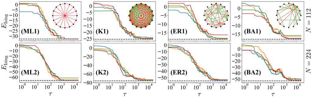
FIG. 3. Ising energy from the OPO phases during the round trips for (ML1),(ML2) M¨ obius ladder, (K1),(K2) complete graph, (ER1),(ER2) Erd˝ os-R´ enyi graph, and (BA1),(BA2) Barab´ asi-Albert graph. Upper panels refer to N = 112, while lower panels to N = 224. Different lines refer to different initial conditions. Horizontal black dashed lines mark the GS energy found by diagonalizing J for ML, and the minimal energy found by Metropolis annealing for K, ER, and BA. The insets in the upper panels depict the different connectivities in the four cases (black dots are nodes, and red and green lines depict negative and positive edge weights, respectively), where N = 16 is used for illustration purposes only.
<details>
<summary>Image 3 Details</summary>
### Visual Description
## Chart: Energy vs. Time for Different Network Models
### Overview
The image presents a series of eight line charts, arranged in a 2x4 grid. Each chart depicts the evolution of "E_ising" (energy) over time (τ) for different network models and network sizes (N). Each chart also includes a small circular diagram representing the network structure. The charts are labeled ML1, K1, ER1, BA1, ML2, K2, ER2, and BA2.
### Components/Axes
* **Y-axis:** Labeled "E_ising", ranging from approximately -35 to 0 in the top row and -60 to 0 in the bottom row. The scale is linear.
* **X-axis:** Labeled "τ" (tau), representing time. The scale is logarithmic, spanning from 10⁰ to 10⁴.
* **Legends:** Each chart contains four colored lines, representing different initial conditions or realizations of the model. The colors are:
* Blue
* Green
* Red
* Orange
* **Network Diagrams:** Small circular diagrams are positioned above each line chart, visually representing the network structure for each model.
* **Labels:** Each chart is labeled with a unique identifier (ML1, K1, ER1, BA1, ML2, K2, ER2, BA2).
* **N values:** The rightmost column of charts is labeled "N = 12" and "N = 224", indicating the network size.
* **Horizontal dashed line:** A horizontal dashed line is present in each chart at approximately y = -25 in the top row and y = -50 in the bottom row.
### Detailed Analysis or Content Details
**ML1 (N=12):**
* The blue line starts at approximately 0 and decreases rapidly to around -30, then plateaus.
* The green line starts at approximately 0 and decreases to around -25, then plateaus.
* The red line starts at approximately 0 and decreases to around -20, then plateaus.
* The orange line starts at approximately 0 and decreases to around -15, then plateaus.
**K1 (N=12):**
* The blue line starts at approximately 0 and decreases to around -15, then plateaus.
* The green line starts at approximately 0 and decreases to around -20, then plateaus.
* The red line starts at approximately 0 and decreases to around -25, then plateaus.
* The orange line starts at approximately 0 and decreases to around -20, then plateaus.
**ER1 (N=12):**
* The blue line starts at approximately 0 and decreases to around -10, then plateaus.
* The green line starts at approximately 0 and decreases to around -15, then plateaus.
* The red line starts at approximately 0 and decreases to around -20, then plateaus.
* The orange line starts at approximately 0 and decreases to around -15, then plateaus.
**BA1 (N=12):**
* The blue line starts at approximately 0 and decreases to around -10, then plateaus.
* The green line starts at approximately 0 and decreases to around -15, then plateaus.
* The red line starts at approximately 0 and decreases to around -20, then plateaus.
* The orange line starts at approximately 0 and decreases to around -15, then plateaus.
**ML2 (N=224):**
* The blue line starts at approximately 0 and decreases to around -30, then plateaus.
* The green line starts at approximately 0 and decreases to around -40, then plateaus.
* The red line starts at approximately 0 and decreases to around -45, then plateaus.
* The orange line starts at approximately 0 and decreases to around -35, then plateaus.
**K2 (N=224):**
* The blue line starts at approximately 0 and decreases to around -20, then plateaus.
* The green line starts at approximately 0 and decreases to around -40, then plateaus.
* The red line starts at approximately 0 and decreases to around -60, then plateaus.
* The orange line starts at approximately 0 and decreases to around -50, then plateaus.
**ER2 (N=224):**
* The blue line starts at approximately 0 and decreases to around -10, then plateaus.
* The green line starts at approximately 0 and decreases to around -20, then plateaus.
* The red line starts at approximately 0 and decreases to around -40, then plateaus.
* The orange line starts at approximately 0 and decreases to around -30, then plateaus.
**BA2 (N=224):**
* The blue line starts at approximately 0 and decreases to around -10, then plateaus.
* The green line starts at approximately 0 and decreases to around -20, then plateaus.
* The red line starts at approximately 0 and decreases to around -40, then plateaus.
* The orange line starts at approximately 0 and decreases to around -30, then plateaus.
### Key Observations
* All charts show a decrease in E_ising over time, indicating the system is reaching a lower energy state.
* The rate of energy decrease varies between models and initial conditions.
* Larger network sizes (N=224) generally exhibit lower final energy values compared to smaller networks (N=12).
* The orange lines consistently reach the lowest energy levels in most charts.
* The horizontal dashed lines appear to represent a baseline or threshold energy level.
### Interpretation
The charts demonstrate the energy dynamics of different network models (ML, K, ER, BA) as a function of time. The models likely represent different network generation algorithms (e.g., ML = Modified Lloyd, K = complete graph, ER = Erdős–Rényi, BA = Barabási–Albert). The decreasing E_ising values suggest the systems are evolving towards equilibrium. The differences in energy levels and decay rates between models indicate varying degrees of stability and energy dissipation. The larger network sizes (N=224) generally reach lower energy states, suggesting that larger networks have more opportunities to minimize their energy. The consistent performance of the orange lines could indicate a specific initial condition or parameter setting that favors lower energy configurations. The horizontal dashed lines might represent a theoretical minimum energy or a critical threshold for the system. The network diagrams provide a visual representation of the connectivity patterns in each model, which likely influence their energy dynamics. The data suggests that the network structure significantly impacts the system's energy landscape and its ability to reach a stable state.
</details>
where B 0 is the uniform pump amplitude at the entrance of the NLM, which provides the gain. There are two sources of loss: The SLM transmission function Q , and measurement and intrinsic loss encoded in R out . The balance between gain and losses during the initial round trips defines the value B 0 , th of the oscillation threshold: B 0 , th = -log[ R out ρ ( Q )] /κL , where ρ ( Q ) is the spectral radius of Q .
We shine the NLM with a pump laser at λ p = 532nm with spot radius w 0 = 100 µ m. The physical properties of the NLM are encoded in χ (2) , λ s , and n (determining κ ), and L . Here, we use χ (2) = 10 -11 m / V, λ s = 1064nm, n = 2 ( κ 1 . 48 × 10 -5 V -1 ), and L = 10cm, which defines the characteristic length scale in our simulations. To integrate Eq. (1), we use as characteristic field amplitude A 0 6 . 77 × 10 3 V / m, which yields the numerical rescaled nonlinear constant ˜ κ := κz 0 A 0 = 10 -2 , and thus integrate Eq. (1) for z ∈ [0 , 1] (in units of L ). At τ = 0, the signal consists of white noise with amplitude 10 -3 A 0 .
The SLM transmission function Q is written by including self-interaction and off-diagonal coupling terms J , which is a real symmetric matrix: Q = a 1 + b J , where 1 is the identity matrix. Since the SLM provides phase and amplitude modulation, Q ij is in general a complex number with | Q ij | < 1. The lossy nature of the SLM implies ρ ( Q ) < 1. To benchmark our proof-of-principle machine, we simulate N = 112 coupled OPOs and solve the MAX-CUT problem for four undirected graphs for which the optimization problem belongs to different classes of computational complexity (P and NP-hard) [41, 50]: The M¨ obius ladder (ML) [51], which is a circulant P-graph realized with the scheme in Fig. 1 b , and three NP-hard graphs, specifically the random Erd˝ os-R´ enyi (ER) and scale-free Barab´ asi-Albert (BA) graphs [52] with approximately 20% edge density, and the random complete (K) graph [53], realized with the scheme in Fig. 1 c . For
TABLE I. Values of the pump amplitude B 0 at the entrance of the NLM used in the simulation, for the data in Fig. 3.
| | ML | K | ER | BA |
|---------|----------------|-----------------|----------------|----------------|
| N = 112 | 1 . 2 B 0 , th | 1 . 33 B 0 , th | 1 . 3 B 0 , th | 1 . 3 B 0 , th |
| N = 224 | 1 . 2 B 0 , th | 1 . 36 B 0 , th | 1 . 3 B 0 , th | 1 . 3 B 0 , th |
the ML, the nonzero entries of J are J i,i +1 = α and J i,i + N/ 2 = α , with negative α . For the ER and BA graphs, J ij = 0 , ± β , where the three values are randomly chosen from the appropriate probability distribution to yield the chosen edge density [52], while for the K graph, J ij = ± γ , where the sign is randomly chosen with equal probability. We set a = 0 . 96, b = 0 . 04, α = -0 . 2, and β = 0 . 05, and γ = 0 . 03, for which ρ ( Q ) 0 . 98 in all cases. In this setup, by setting T out = √ 0 . 1, we obtain threshold pump powers P th ∼ 200 mW.
We first show in Fig. 2 the histogram of the time evolution of (a) Re[ A j,τ ], and (b) Im[ A j,τ ], for short times, specifically for ML. As evident, Re[ A j,τ ] is exponentially amplified, whereas Im[ A j,τ ] is instead suppressed. This confirms that the system is correctly in the phase-dependent amplification regime. Next, we simulate the OPO dynamics for the chosen graphs and compute the Ising energy from OPO phase configuration as E Ising ( τ ) = -(1 / 2) ∑ ij J ij σ i ( τ ) σ j ( τ ), where σ i ( τ ) = sgn( A i,τ ) and sgn( · ) is the sign function. We compare the energy for two different values of N , namely N = 112 and N = 224. The result is shown in Fig. 3. Different panels refer to different graphs and different N as in the labels, using the values of the pump amplitude B 0 at the entrance of the NLM given in Table I. Different solid lines refer to different initial conditions of the fields. The black horizontal lines mark the minimal Ising energy: The P
nature of the problem with the ML allows to find this value exactly by diagonizaling J , selecting the eigenvector with maximal eigenvalue [41]. Instead, for the NP-hard cases of K, ER, and BA, we estimate the minimal value by a Metropolis annealing algorithm. The fact that the steady-state value of E Ising coincides with the exact minimal value for ML, while sometimes it does not for K, ER, and BA, reflects the different computational complexity of the optimization [41, 50].
The key result in Fig. 3 is that our system approaches a steady state with energy close to the minimum energy of the corresponding Ising Hamiltonian after about 10 3 round trips, for both values of N . Since in our scheme all OPOs evolve in time in parallel, our device allows to use short cavities (typically D ∼ 1 m long) that in turn ensures short round trips times τ RT = 2 nD/c ∼ 10 ns, independent of N . We then estimate the total computational time as approximately 10 µ s. As such, the parallelization of the dynamics allows to envision orders of magnitude shorter computational time compared to existing CIM realizations [32, 33, 54, 55].
## IV. CONCLUSIONS
In conclusion, we propose a fully-optical scalable spatial CIM implementing different connectivities. The binary nature of the signal phase at different points on the wavefront is enforced by the NLM within the parametric cavity, and the spatial discretization of the wavefront is defined by the SLM within the cavity implementing the spin-spin optical coupling. The number of spins that our system encodes critically depends on the specific configuration of the SLM. To implement a fully-programmable
- [1] J. J. Hopfield, 'Neural networks and physical systems with emergent collective computational abilities,' PNAS 79 , 2554-2558 (1982).
- [2] M. Gilli, D. Maringer, and E. Schumann, Numerical Methods and Optimization in Finance (Elsevier Science, 2011).
- [3] Q. Zhang, D. Deng, W. Dai, J. Li, and X. Jin, 'Optimization of culture conditions for differentiation of melon based on artificial neural network and genetic algorithm,' Sci. Rep. 10 , 3524 (2020).
- [4] A. Degasperi, D. Fey, and B. N. Kholodenko, 'Performance of objective functions and optimisation procedures for parameter estimation in system biology models,' npj Syst. Biol. Appl. 3 , 20 (2017).
- [5] M. Ohzeki, S. Okada, M. Terabe, and S. Taguchi, 'Optimization of neural networks via finite-value quantum fluctuations,' Sci. Rep. 8 , 9950 (2018).
- [6] R. M. Karp, 'Reducibility among combinatorial problems,' in Complexity of Computer Computations (1972) pp. 85-103.
- [7] A. Lucas, 'Ising formulations of many NP problems,' Frontiers in Physics 2 , 5 (2014).
CIM, we propose a setup based on the vector-matrix multiplication scheme, where the SLM works in real space of the field. This scheme allows the implementation of any graph, however limiting the number of spins to N ∼ 10 3 due to the redundant encoding of the spin variables on the SLM pixels. We then propose an alternative coupling scheme with the SLM working in momentum space of the field, which allows the implementation of a limited class of graphs but it can host N ∼ 10 6 spins.
The all-optical nature of our machine presents a step towards the realization of large-scale scalable CIMs. First, in our proposal, both the OPO dynamics and their mutual coupling are fully parallelized, which makes the reach for the optimal solution size independent. Second, the parallel encoding of all OPOs allows for short cavity lengths, and thus drastically smaller computational time, compared to state-of-the art realizations with hybrid electronic-optical setups, where the OPOs are arranged as a temporal sequence of pulses and cavity lengths of approximately 1 km are needed. Another important advance of our proposal compared to existing realizations is that no measurement is performed during the time evolution to realize the mutual interaction. This makes our machine suitable to study fundamental features of coupled OPOs beyond optimization, like the emergence of robust macroscopic quantum entanglement [56, 57].
## ACKNOWLEDGEMENTS
We acknowledge funding from Sapienza Ricerca, PRIN PELM (20177PSCKT), QuantERA ERA-NET Co-fund (Grant No. 731473, Project QUOMPLEX), H2020 PhoQus Project (Grant No. 820392).
- [8] F. Barahona, 'On the computational complexity of Ising spin glass models,' J. Phys. A 15 , 3241-3253 (1982).
- [9] T. Byrnes, K. Yan, and Y. Yamamoto, 'Accelerated optimization problem search using Bose-Einstein condensation,' New J. Phys. 13 , 113025 (2011).
- [10] T. Byrnes, S. Koyama, K. Yan, and Y. Yamamoto, 'Neural networks using two-component Bose-Einstein condensates,' Sci. Rep. 3 , 2531 (2013).
- [11] M. W. Johnson, M. H. S. Amin, S. Gildert, T. Lanting, F. Hamze, N. Dickson, R. Harris, A. J. Berkley, J. Johansson, P. Bunyk, E. M. Chapple, C. Enderud, J. P. Hilton, K. Karimi, E. Ladizinsky, N. Ladizinsky, T. Oh, I. Perminov, C. Rich, M. C. Thom, E. Tolkacheva, C. J. S. Truncik, S. Uchaikin, J. Wang, B. Wilson, and G. Rose, 'Quantum annealing with manufactured spins,' Nature 437 , 194-198 (2011).
- [12] K. Kim, M.-S. Chang, S. Korenblit, R Islam, E. E. Edwards, J. K. Freericks, G.-D. Lin, L.-M. Duan, and C. Monroe, 'Quantum simulation of frustrated Ising spins with trapped ions,' Nature 465 , 590-593 (2010).
- [13] J. W. Britton, B. C. Sawyer, A. C. Keith, C.-C. J. Wang, J. K. Freericks, H. Uys, M. J. Biercuk, and
J. J. Bollinger, 'Engineered two-dimensional Ising interactions in a trapped-ion quantum simulator with hundreds of spins,' Nature 484 , 489-492 (2012).
- [14] A. D. King, W. Bernoudy, J. King, A. J Berkley, and T. Lanting, 'Emulating the coherent Ising machine with a mean-field algorithm,' arXiv:1806.08422 (2018).
- [15] E. S. Tiunov, A. E. Ulanov, and A. I. Lvovsky, 'Annealing by simulating the coherent Ising machine,' Opt. Express 27 , 10288-10295 (2019).
- [16] H. Goto, K. Tatsumura, and A. R. Dixon, 'Combinatorial optimization by simulating adiabatic bifurcations in nonlinear Hamiltonian systems,' Sci. Adv. 5 , eaav2372 (2019).
- [17] K. Tatsumura, M. Yamasaki, and H. Goto, 'Scaling out Ising machines using a multi-chip architecture for simulated bifurcation,' Nat. Electron. 4 , 208-217 (2021).
- [18] J. Chou, S. Bramhavar, S. Ghosh, and W. Herzog, 'Analog coupled oscillator based weighted Ising machine,' Sci. Rep. 9 , 14786 (2019).
- [19] F. B¨ ohm, G. Verschaffelt, and G. Van der Sande, 'A poor man's coherent Ising machine based on optoelectronic feedback systems for solving optimization problems,' Nat. Commun. 10 , 3538 (2019).
- [20] N. G. Berloff, M. Silva, K. Kalinin, A. Askitopoulos, J. D. T¨ opfer, P. Cilibrizzi, W. Langbein, and P. G. Lagoudakis, 'Realizing the classical XY Hamiltonian in polariton simulators,' Nat. Mat. 16 , 1120-1126 (2017).
- [21] K. P. Kalinin and N. G. Berloff, 'Simulating Ising and n -state planar Potts models and external fields with nonequilibrium condensates,' Phys. Rev. Lett. 121 , 235302 (2018).
- [22] K. P. Kalinin and N. G. Berloff, 'Global optimization of spin Hamiltonians with gain-dissipative systems,' Sci. Rep. 8 , 17791 (2018).
- [23] S. Utsunomiya, K. Takata, and Y. Yamamoto, 'Mapping of Ising models onto injection-locked laser systems,' Opt. Express 19 , 18091-18108 (2011).
- [24] C. Tradonsky, I. Gershenzon, V. Pal, R. Chriki, A. A. Friesem, O. Raz, and N. Davidson, 'Rapid laser solver for the phase retrieval problem,' Sci. Adv. 5 , 10 (2019).
- [25] Z. Wang, A. Marandi, K. Wen, R. L. Byer, and Y. Yamamoto, 'Coherent Ising machine based on degenerate optical parametric oscillators,' Phys. Rev. A 88 , 063853 (2013).
- [26] A. Marandi, Z. Wang, K. Takata, R. L. Byer, and Y. Yamamoto, 'Network of time-multiplexed optical parametric oscillators as a coherent Ising machine,' Nat. Photonics 8 , 937 (2014).
- [27] K. Takata, A. Marandi, R. Hamerly, Y. Haribara, D. Maruo, S. Tamate, H. Sakaguchi, S. Utsonomiya, and Y. Yamamoto, 'A 16-bit coherent Ising machine for onedimensional ring and cubic graph problems,' Sci. Rep. 6 , 34089 (2016).
- [28] T. Inagaki, K. Inaba, R. Hamerly, K. Inoue, Y. Yamamoto, and H. Takesue, 'Large-scale Ising spin network based on degenerate optical parametric oscillators,' Nat. Photonics 10 , 415-419 (2016).
- [29] R. Hamerly, K. Inaba, T. Inagaki, H. Takesue, Y. Yamamoto, and H. Mabuchi, 'Topological defect formation in 1D and 2D spin chains realized by network of optical parametric oscillators,' Int. J. Mod. Phys. B 30 , 1630014 (2016).
- [30] W. R. Clements, J. J. Renema, Y. H. Wen, H. M. Chrzanowski, W. S. Kolthammer, and I. A. Walms-
ley, 'Gaussian optical Ising machines,' Phys. Rev. A 96 , 043850 (2017).
- [31] T. Wang and J. Roychowdhury, 'Oscillator-based Ising machine,' arXiv:1709.08102 (2017).
- [32] Takahiro Inagaki, Yoshitaka Haribara, Koji Igarashi, Tomohiro Sonobe, Shuhei Tamate, Toshimori Honjo, Alireza Marandi, Peter L. McMahon, Takeshi Umeki, Koji Enbutsu, Osamu Tadanaga, Hirokazu Takenouchi, Kazuyuki Aihara, Ken-ichi Kawarabayashi, Kyo Inoue, Shoko Utsunomiya, and Hiroki Takesue, 'A coherent Ising machine for 2000-node optimization problems,' Science 354 , 603-606 (2016).
- [33] R. Hamerly, T. Inagaki, P. L. McMahon, D. Venturelli, A. Marandi, T. Onodera, E. Ng, C. Langrock, K. Inaba, T. Honjo, K. Enbutsu, T. Umeki, R. Kasahara, S. Utsunomiya, S. Kako, K. Kawarabayashi, R. L. Byer, M. M. Fejer, H. Mabuchi, D. Englund, E. Rieffel, H. Takesue, and Y. Yamamoto, 'Experimental investigation of performance differences between coherent Ising machines and a quantum annealer,' Sci. Adv. 5 , eaau0823 (2019).
- [34] D. Pierangeli, G. Marcucci, and C. Conti, 'Large-scale photonic Ising machine by spatial light modulation,' Phys. Rev. Lett. 122 , 213902 (2019).
- [35] L. Bello, M. Calvanese Strinati, E. G. Dalla Torre, and A. Pe'er, 'Persistent coherent beating in coupled parametric oscillators,' Phys. Rev. Lett. 123 , 083901 (2019).
- [36] T. Wang and J. Roychowdhury, 'Oim: Oscillator-based Ising machines for solving combinatorial optimisation problems,' in Unconventional Computation and Natural Computation (Springer International Publishing, Cham, 2019) pp. 232-256.
- [37] Y. Okawachi, M. Yu, J. K. Jang, X. Ji, Y. Zhao, B. Y. Kim, M. Lipson, and A. L. Gaeta, 'Demonstration of chip-based coupled degenerate optical parametric oscillators for realizing a nanophotonic spin-glass,' Nat. Commun. 11 , 4119 (2020).
- [38] D. Pierangeli, G. Marcucci, and C. Conti, 'Adiabatic evolution on a spatial-photonic Ising machine,' Optica 7 , 1535-1543 (2020).
- [39] E. Goto, 'The parametron, a digital computing element which utilizes parametric oscillation,' Proc. IRE 47 , 1304 (1959).
- [40] J. W. F. Woo and R. Landauer, 'Fluctuations in a parametrically excited subharmonic oscillator,' IEEE J. Quantum Electron QE-7 , 435 (1971).
- [41] M. Calvanese Strinati, L. Bello, E. G. Dalla Torre, and A. Pe'er, 'Can nonlinear parametric oscillators solve random Ising models?' Phys. Rev. Lett. 126 , 143901 (2021).
- [42] M. Erementchouk, A. Shukla, and P. Mazumder, 'Computational capabilities of nonlinear oscillator networks,' arXiv:2105.07591 (2021).
- [43] Yoshitaka Haribara, Shoko Utsunomiya, and Yoshihisa Yamamoto, 'A coherent Ising machine for max-cut problems: Performance evaluation against semidefinite programming and simulated annealing,' in Principles and Methods of Quantum Information Technologies , edited by Yoshihisa Yamamoto and Kouichi Semba (Springer Japan, Tokyo, 2016) pp. 251-262.
- [44] D. Pierangeli, M. Rafayelyan, C. Conti, and S. Gigan, 'Scalable spin-glass optical simulator,' Phys. Rev. Applied 15 , 034087 (2021).
- [45] S. Kumar, H. Zhang, and Y.-P. Huang, 'Large-scale Ising emulation with four body interaction and all-to-all connections,' Comm. Phys. 3 , 108 (2020).
- [46] P. J. Davis, Circulant Matrices , Chelsea Publishing Series (Chelsea, 1994).
- [47] J. Spall, X. Guo, T. D. Barrett, and A. I. Lvovsky, 'Fully reconfigurable coherent optical vector-matrix multiplication,' Opt. Lett. 45 , 5752-5755 (2020).
- [48] R.W. Boyd, Nonlinear Optics (Elsevier Science, 2008).
- [49] M. Calvanese Strinati, I. Aharonovich, S. Ben-Ami, E. G. Dalla Torre, L. Bello, and A. Pe'er, 'Coherent dynamics in frustrated coupled parametric oscillators,' New J. Phys. 22 , 085005 (2020).
- [50] K. P. Kalinin and N. G. Berloff, 'Complexity continuum within Ising formulation of NP problems,' arXiv:2008.00466 (2020).
- [51] R. K. Guy and F. Harary, 'On the M¨ obius ladders,' Canad. Math. Bull. 10 , 493-496 (1967).
- [52] R. Albert and A.-L. Barab´ asi, 'Statistical mechanics of complex networks,' Rev. Mod. Phys. 74 , 47-97 (2002).
- [53] D. Gries and F. B. Schneider, A Logical Approach to Discrete Math (Springer-Verlag, 1993).
- [54] Y. Haribara, H. Ishikawa, S. Utsunomiya, K. Aihara, and Y. Yamamoto, 'Performance evaluation of coherent Ising machines against classical neural networks,' Quantum Sci. Technol 2 , 044002 (2017).
- [55] Y. Yamamoto, K. Aihara, T. Leleu, K. Kawarabayashi, S. Kako, M. Fejer, K. Inoue, and H. Takesue, 'Coherent Ising machines-optical neural networks operating at the quantum limit,' njp Quantum Information 3 , 49 (2017).
- [56] S. Kiesewetter and P. D. Drummond, 'Weighted phasespace simulations of feedback coherent Ising machines,' arXiv:2105.04190 (2021).
- [57] Z.-Y. Zhou, C. Gneiting, J. Q. You, and F. Nori, 'Generating and detecting entangled cat states in dissipatively coupled degenerate optical parametric oscillators,' Phys. Rev. A 104 , 013715 (2021).