## Abductive Inference and C. S. Peirce: 150 Years Later
Subhadeep (DEEP) Mukhopadhyay
Email:
deep@unitedstatalgo.com
## Abstract
Two pillars of the paper . This paper is about two things: (i) Charles Sanders Peirce (1837-1914)-an iconoclastic philosopher and polymath who is among the greatest of American minds. (ii) Abductive inference-a term coined by C. S. Peirce, which he defined as 'the process of forming explanatory hypotheses. It is the only logical operation which introduces any new idea.'
Abductive inference and quantitative economics . Abductive inference plays a fundamental role in empirical scientific research as a tool for discovery and data analysis. Heckman and Singer (2017) strongly advocated 'Economists should abduct .' Arnold Zellner (2007) stressed that 'much greater emphasis on reductive [abductive] inference in teaching econometrics, statistics, and economics would be desirable.' But currently, there are no established theory or practical tools that can allow an empirical analyst to abduct. This paper attempts to fill this gap by introducing new principles and concrete procedures to the Economics and Statistics community. I termed the proposed approach as Abductive Inference Machine ( AIM ).
The historical Peirce's experiment . In 1872, Peirce conducted a series of experiments to determine the distribution of response times to an auditory stimulus, which is widely regarded as one of the most significant statistical investigations in the history of nineteenth-century American mathematical research (Stigler, 1978). On the 150th anniversary of this historical experiment, we look back at the Peircean-style abductive inference through a modern statistical lens. Using Peirce's data, it is shown how empirical analysts can abduct in a systematic and automated manner using AIM .
Keywords : Abductive inference machine; Artificial intelligence; Density sharpening; Informative component analysis; Problem of surprise; Laws of discovery; Self-corrective models.
## 1. INTRODUCTION
Charles Sanders Peirce (1839-1914), America's greatest philosopher of science, was also a brilliant statistician and experimental scientist. For 32 years, from 1859 until 1891, he worked for the United States Coast and Geodetic Survey 1 . During this time, he developed an unfailing passion for experimental research. He was deeply involved in developing theoretical and practical methods for acquiring high-precision scientific measurements, which ultimately earned him an international reputation as an expert in 'measurement error' in physics. Robert Crease (2009), a philosopher and historian of science, noted: 'His [Peirce's] work helped remove American metrology from under the British shadow and usher in an American tradition.'
## Pierce's 1872 Experiment
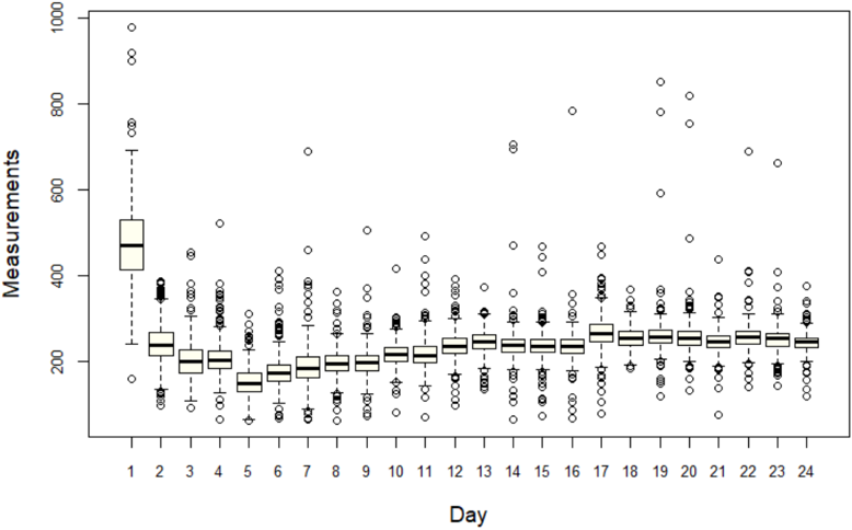
Figure 1: First look at Peirce's auditory response data. The x-axis denotes 24 different days of experiments and the y-axis displays the data of individual experiment as boxplot.
<details>
<summary>Image 1 Details</summary>
### Visual Description
\n
## Box Plot: Measurements vs. Day
### Overview
The image presents a box plot visualizing the distribution of "Measurements" across 24 "Days". The plot displays the median, quartiles, and outliers for each day's measurements. Individual data points are also plotted on top of the box plots.
### Components/Axes
* **X-axis:** "Day", ranging from 1 to 24. The axis is labeled at each integer value.
* **Y-axis:** "Measurements", ranging from 0 to 1000, with markings at 100-unit intervals.
* **Box Plots:** Each day (1-24) has a corresponding box plot representing the distribution of measurements for that day.
* **Data Points:** Individual circles represent individual measurement values for each day.
* **Outliers:** Data points falling outside the "whiskers" of the box plots are considered outliers and are plotted as individual circles.
### Detailed Analysis
The box plots show the following approximate characteristics for each day:
* **Day 1:** The median is approximately 240. The interquartile range (IQR) extends from roughly 180 to 320. There are several outliers, with the highest measurement reaching approximately 800.
* **Day 2:** The median is approximately 220. The IQR extends from roughly 160 to 280. There are several outliers, with the highest measurement reaching approximately 700.
* **Day 3:** The median is approximately 200. The IQR extends from roughly 140 to 260. There are several outliers, with the highest measurement reaching approximately 600.
* **Days 4-24:** The median values generally hover around 180-220. The IQR is relatively consistent across these days, ranging from approximately 140 to 260. Outliers are present on most days, but their frequency and magnitude vary. Days 19 and 22 show a higher concentration of outliers, with some values exceeding 700.
**Specific Data Points (Approximate):**
* Day 7: Median ~ 190, IQR ~ 150-250
* Day 10: Median ~ 180, IQR ~ 140-240
* Day 14: Median ~ 190, IQR ~ 150-260
* Day 18: Median ~ 200, IQR ~ 160-280
* Day 21: Median ~ 190, IQR ~ 150-260
The box plots for days 1-3 are noticeably taller than those for days 4-24, indicating greater variability in measurements during the first three days.
### Key Observations
* **Higher Variability Early On:** The first three days exhibit significantly higher variability in measurements compared to the rest of the period.
* **Outlier Presence:** Outliers are consistently present throughout the 24-day period, suggesting that extreme measurement values occur regularly.
* **Stable Median:** The median measurement remains relatively stable across all days, fluctuating within a narrow range of approximately 180-240.
* **Days 19 & 22:** These days show a higher concentration of outliers, suggesting potentially unusual events or conditions on those days.
### Interpretation
The data suggests a period of initial instability or adjustment (days 1-3) followed by a more stable measurement pattern (days 4-24). The consistent presence of outliers indicates that while the central tendency of the measurements remains relatively constant, there are occasional extreme values that deviate significantly from the norm. The higher outlier frequency on days 19 and 22 warrants further investigation to determine the underlying causes.
The box plot effectively visualizes the distribution of measurements, highlighting the central tendency, spread, and presence of outliers for each day. This type of visualization is useful for identifying patterns, comparing distributions, and detecting anomalies in the data. The data could represent any time-series measurement, such as daily temperature, stock prices, or sensor readings. The initial high variability could indicate a system settling into a stable state, or the influence of external factors that diminish over time.
</details>
1872 Experimental Data . In 1872, he conducted a series of famous experiments to determine the distribution of response times to an auditory stimulus. He measured the time that elapsed between the making of a sharp sound and the record of reception of the sound by an observer,
1 U. S. Coast and Geodetic Survey was established on February 10, 1807, by President Thomas Jefferson. It was the nation's first civilian scientific agency.
employing a Hipp chronoscope (some kind of sophisticated clock). Fig. 1 shows the dataset, which consists of roughly 500 measurements (recorded in nearest milliseconds) each day for k 24 different days 2 . Note that the first-day observations are systematically different from others (also called systematic bias), and the inconsistency was due to the lack of experience of the observer, which was corrected on the next day. The next 23 days show much more consistent (comparable) measurements.
## 2. GAUSS' LAW OF ERROR
What observation has to teach us is [density] function, not a mere number.
$$- C . S . P e i r c e ( 1 8 7 3 )$$
Deciphering the Law of Errors . Peirce's actual motivation for doing the experiment was to study the probabilistic laws of fluctuations (also called errors) in the measurements and to investigate how response time distributions differ from the standard Gauss' law.
Nineteenth-century statistical learning . Peirce (1873) presented a detailed empirical investigation of the reaction-time densities for each day. He was driven by two goals: to understand the shape of the reaction time densities and to compare them with the expected Gaussian distribution. His approach had a remarkably modern conceptual basis: first, he developed smooth kernel density-type probability density estimates to understand the shape of error distributions 3 ; second, he performed a goodness-of-fit (GOF) type assessment through visual comparison between the shape of Gaussian distribution and the nonparametrically estimated densities 4 , and concluded that the reaction-time distributions 'differed very little from' the expected normal probability law 5 .
2 For further details on the experimental setup and the full dataset, consult the online Peirce Edition Project: vol 3, p. 133-160 of the chronological edition (Peirce, 2009). It's also available in the R-package quantreg .
3 Peirce made a pioneering contribution to American statistics by developing the concepts that underpin nonparametric density estimation.
4 However, at that time no theory of GOF was available. It took 30 more years for an English mathematician, Karl Pearson, to make the breakthrough contribution in developing the formal language of the GOF.
5 The term 'normal distribution' was coined by Peirce.
Twentieth-century statistical learning . Almost sixty years later, the same dataset was reanalyzed by Wilson and Hilferty (1929), and they came to a very different conclusion. Wilson and Hilferty performed a battery of tests to verify the appropriateness of the normal distribution. For each series of measurements, they computed 23 statistics (e.g., mean, standard deviation, skewness, kurtosis, interquartile range, etc.) to justify substantial departures from Gaussianity. Interestingly, without any formal statistical test, simply by carefully looking at the boxplots in Fig. 1, we can see the presence of significant skewness (the median cuts the boxes into two unequal pieces), heavy-tailedness (long whiskers relative to the box length), and ample outlying observations-which is good enough to suspect the adequacy of Gaussian distribution as a model for the data.
Remark 1. The non-Gaussian nature of the error distribution of scientific measurements is hardly surprising 6 - in fact, it is the norm, not the exception (Bailey, 2017), which arises primarily because it is hard to control all the factors of a complex measurement process. But what is startling is that even Peirce's experiment, a simple investigation of recording response times with the same instrument by the same person under more or less similar conditions, can produce so much heterogeneity.
' Does statistics help in the search for an alternative hypothesis? There is no codified statistical methodology for this purpose. Text books on statistics do not discuss either in general terms or through examples how to elicit clues from data to formulate an alternative hypothesis or theory when a given hypothesis is rejected. '
- C. R. Rao (2001)
Revised Goal: From Testing to Discovery . Confirmatory analysis through hypothesis testing provides investigators absolutely no clues on what might actually be going on. 7 Simply rejecting a hypothesis-saying that it is non-Gaussian-does not add any new insight into the
6 Even Wilson and Hilferty (1929) noted the same: 'according to our previous experience such long series of observations generally reveal marked departures from the normal law.'
7 An average statistician uses data to confirm or reject a particular theory/model. A competent statistician uses data to sharpen their theory/model.
underlying laws of error. Thus, our focus will be on developing a data analysis technique that can identify the most questionable aspects of the existing model and can also provide concrete recommendations on how to rectify those deficiencies in order to build a better and more realistic model for the measurement uncertainties.
## 3. THE PROBLEM OF SURPRISE
It is not enough to, look for what we anticipate. The greatest gains from data come from surprises. - John Tukey (1972)
Modeling the Surprise . All empirical laws are approximations of reality-sometimes good, sometimes bad. We will be fooling ourselves if we think there is a single best model that fits Peirce's experimental data. Any statistical model, irrespective of how sophisticated it is, should be ready to be surprised by data. The goal of empirical modeling is to develop a general strategy for describing how a model should react and adapt itself to reduce the surprise.
Without surprise, there is no discovery. The 'process' of discovering new knowledge from data starts by answering the following questions: Is there anything surprising in the data? If so, what makes it surprising? How should the current model react to the surprise? How can it modify itself to rationalize the empirical surprise? To develop a model and principle for statistical discovery, we need to first address these fundamental data modeling questions. In subsequent sections, we develop one such general theory.
Basic notations used throughout the paper: X is a continuous random variable with cdf F p x q , pdf f p x q . The quantile function is given by Q p u q F 1 p u q . Expectation with respect to the initial working model F 0 p x q is abbreviated as E 0 p ψ p X qq : ‡ ψ d F 0 , and expectation with respect to the empirical r F is simply written as r E p ψ p X qq : ‡ ψ d r F . The inner product of two functions ψ 1 and ψ 2 in L 2 p dF 0 q will be denoted by x ψ 1 , ψ 2 y F 0 : ‡ ψ 1 ψ 2 d F 0 .
## 4. A MODEL FOR EMPIRICAL DISCOVERY
There is no established practice for dealing with surprise, even though surprise is an everyday occurrence. Is there a best way to respond to empirical surprises?
- Heckman and Singer (2017)
## 4.1 A Dyadic Meta-Model
Science is a 'self-corrective' enterprise that seeks new knowledge by refining the known. 8 The same is true for statistical modeling: it explores and discovers unknown patterns by smartly utilizing the known (expected) model. In the following, we formalize this general principle.
Definition 1 (A Dyadic Meta-Model) . X be a continuous random variable with true unknown density f p x q . Let f 0 p x q represents a possibly misspecified predesignated working model for X , whose support includes the support of f p x q . Then the following density decomposition formula holds:
$$f ( x ) \, = \, f _ { 0 } ( x ) \, d \left ( F _ { 0 } ( x ) ; F _ { 0 } , F \right ) ,$$
where the d p u ; F 0 , F q is defined as
$$d ( u ; F _ { 0 } , F ) = \frac { f ( F _ { 0 } ^ { - 1 } ( u ) ) } { f _ { 0 } ( F _ { 0 } ^ { - 1 } ( u ) ) } , \, 0 < u < 1 , \quad ( 2 )$$
which is called 'comparison density' because it compares the initial model-0 f 0 p x q with the true f p x q and it integrates to one:
$$\int _ { 0 } ^ { 1 } d ( u ; F _ { 0 } , F ) \, d u \, = \, \int _ { x } d ( F _ { 0 } ( x ) ; F _ { 0 } , F ) \, d F _ { 0 } ( x ) \, = \, \int _ { x } \left ( f ( x ) / f _ { 0 } ( x ) \right ) \, d F _ { 0 } ( x ) \, = \, 1 .$$
To simplify the notation, d p F 0 p x q ; F 0 , F q will be abbreviated as d 0 p x q . One can view (1) as a 'meta-model'-a model comprising two sub-models that blends existing imprecise knowledge f 0 p x q with new empirical knowledge d 0 p x q to provide us complete picture of the uncertainty.
8 According to Peirce, every branch of scientific inquiry exhibits 'the vital power of self-correction' that permits us to make progress and grow our knowledge; see, Burch and Parker (2022).
The above density representation formula can be interpreted from many different angles:
1. Model-Editing Tool . The dyadic model provides a general statistical mechanism for designing a 'better' model by editing or sharpening the existing version. For that reason, we call d the density-sharpening function (DSF). Next section presents how to learn DSF from data. The d -modulated repaired f 0 -density in Eq. (1) will be referred to d -sharp f 0 .
2. Surprisal Function . The process of data-driven discovery starts with a surprise-a deviation between the data and the expected model. The DSF d p u ; F 0 , F q gets activated only when model-0 encounters surprise, and its shape encodes the nature of surprise. When there is no surprise, d p u ; F 0 , F q takes the shape of a 'flat' uniform density.
Surprise to information gain : It is not enough to simply detect an empirical surprise. For statistical learning, it is critical to know: What information can we gain from the observed surprise? And how can we use that information to revise our initial model of reality? The density-sharpening function d p u ; F 0 , F q provides a pathway from surprise to information gain that bridges the gap between the initial belief and knowledge.
3. Simon's Means-Ends Analysis . The model (1) interacts with the outer data environment through two information channels:
- Afferent (or 'inward') information: it captures and represents the ' difference ' between the desired and present model using d 0 p x q 9 .
- Efferent (or 'outward') information: it intelligently searches and provides the best course of ' actions ' that changes the present model through (1) to reduce the difference 10 .
Herbert Simon (1988) noted that any general-purpose computational learning system must have these two information processing components. Models equipped with this special structure are known as the 'Means-Ends analysis model' in the artificial intelligence community.
9 It would be pointless to waste computational resources on the redundant part of the data.
10 d 0 p x q 'fires' actions when the difference in information content between F 0 and r F reaches a threshold.
4. Detective's Microscope 11 . Information in the data can be broken down into two parts:
Data Information = Anticipated part + Unexpected surprising part. (3)
Model-0 explains the first part, whereas d 0 p x q captures everything that is unexplainable by the initial f 0 p x q . Accordingly, d 0 p x q performs dual tasks: it reveals the incompleteness of our starting assumptions and provides strategies on how to revise it to account for the observed puzzling facts. In short, d p u ; F 0 , F q plays the role of a detective's microscope , permitting data investigators to assemble clues to initiate a systematic search for new explanatory hypotheses that fit the evidence and solve the puzzle.
5. System-1 and System-2 Architecture 12 . In our dyadic model, System-1 is denoted by f 0 p x q that captures the background knowledge component. Model-0 interacts with the environment through System 2 d -function. The DSF d allows model-0 to self-examine its limitations and also offers strategies for self-correcting to adapt to new situations. The DSF plays the role of a 'supervisor' whose goal is model management. It helps the subordinate f 0 to figure out what's missing and how to fix this. Our dyadic model combines both system-1 and system-2 into one integrated modeling system.
6. A Change Agent : The great philosopher Heraclitus taught us that change is the only constant thing in this world. If we believe in this doctrine then we should focus on modeling the change, not the model itself. 13 The dyadic model operationalizes this philosophy by providing a universal law of model evolution: how to produce a useful model by changing an imperfect model-0 in a data-adaptive manner. The rectified f 0 p x q inherits new characteristics through d 0 p x q that give them a better chance of survival in the new data environment.
11 The name was inspired from John Tukey (1977, p. 52)
12 This 'Two Systems' analogy was inspired by Daniel Kahneman's work on 'Thinking, Fast and Slow.'
13 Isaac Newton confronted a similar problem in the mid-1600s: He wanted to describe a falling object, which changes its speed every second. The challenge was: How to describe a 'moving' object? His revolutionary idea was to focus on modeling the 'change,' which led to the development of Calculus and Laws of Motion. Here we are concerned with a similar question: How to change probability distribution when confronted with new data? In our dyadic model (1), the sharpening function d provides the necessary 'push to change.'
## 4.2 A Robust Nonparametric Estimation Method
To operationalize the density-sharpening law, we need to estimate from data the function d 0 p x q , which is the cause of change in the state of a probability distribution. We describe a theory of robust nonparametric estimation whose core concepts and methodological tools are introduced in a 'programmatic' style-making it easy to translate the theory into a concrete algorithm.
Remark 2 (What are we approximating?) . Before describing the approximation theory, it is vital to emphasize that, unlike traditional nonparametric (or machine learning) methods where the goal is to produce a density estimate p f p x q , in our case, the focus is on estimating the sharpening kernel p d 0 p x q -the 'gap' between theory and measurements. This will provide rational explanations for the surprising facts and, because of Eq. (1), concurrently rectify the initial model f 0 . Also, see sec. 8.
Step 0. Data and Setup . We observe a random sample X 1 , . . . , X n 9 F 0 . By ' 9 ' we mean that F 0 is a tentative (approximate theoretical) model for X that is given to us. And, f p x q denotes the unknown true model from which the data were generated.
Step 1. LP-orthogonal System . Note that DSF d 0 p x q is a function of rankF 0 transform (i.e., probability integral transform with respect to the base measure) F 0 p X q . Hence, one can efficiently approximate d F 0 p x q P L 2 p dF 0 q by expanding it in a Fourier series of polynomials that are function of F 0 p x q and orthonormal with respect to the user-selected base-model f 0 p x q . One such orthonormal system is the LP-family of rank-polynomials (Mukhopadhyay and Fletcher, 2018, Mukhopadhyay, 2017), whose construction is given below.
LP-basis construction for an arbitrary continuous F 0 : Define the first-order LP-basis function as standardized rankF 0 transform:
$$T _ { 1 } ( x ; F _ { 0 } ) \, = \, \sqrt { 1 2 } \left \{ F _ { 0 } ( x ) - 1 / 2 \right \} .$$
Note that E 0 p T 1 p X ; F 0 qq 0 and Var 0 p T 1 p X ; F 0 qq 1. Next, apply Gram-Schmidt procedure
on t T 2 1 , T 3 1 , . . . u to construct a higher-order LP orthogonal system T j p x ; F 0 q :
$$\begin{array} { c c l } T _ { 2 } ( x ; F _ { 0 } ) & = \sqrt { 5 } \left \{ 6 F _ { 0 } ^ { 2 } ( x ) - 6 F _ { 0 } ( x ) + 1 \right \} & & ( 5 ) \end{array}$$
$$\begin{array} { c c l } T _ { 3 } ( x ; F _ { 0 } ) & = & \sqrt { 7 } \left \{ 2 0 F _ { 0 } ^ { 3 } ( x ) - 3 0 F _ { 0 } ^ { 2 } ( x ) + 1 2 F _ { 0 } ( x ) - 1 \right \} & \\ \end{array}$$
$$\begin{array} { r c l } T _ { 4 } ( x ; F _ { 0 } ) & = \sqrt { 9 } \left \{ 7 0 F _ { 0 } ^ { 4 } ( x ) - 1 4 0 F _ { 0 } ^ { 3 } ( x ) + 9 0 F _ { 0 } ^ { 2 } ( x ) - 2 0 F _ { 0 } ( x ) + 1 \right \} , \end{array}$$
and so on. For data analysis, we compute them by executing the Gram-Schmidt process numerically. Hence, there is no need for bookkeeping the explicit formulae of these polynomials. By construction, the LP-sequence of polynomials satisfy the following conditions:
$$\int _ { x } T _ { j } ( x ; F _ { 0 } ) \, d F _ { 0 } \, = \, 0 ; \quad \int _ { x } T _ { j } ( x ; F _ { 0 } ) T _ { k } ( x ; F _ { 0 } ) \, d F _ { 0 } = \delta _ { j k } ,$$
where δ jk is the Kronecker's delta function. The notation for LP-polynomials t T j p x ; F 0 qu is meant to emphasize: (i) they are polynomials of F 0 p x q (not raw x ) and hence are inherently robust. (ii) they are orthonormal with respect to the distribution F 0 , since they satisfy (8). We also define the Unit LP-bases via quantile transform: S j p u ; F 0 q T j p Q 0 p u q ; F 0 q , 0 / u / 1.
Step 2. LP-Fourier Approximation . LP-orthogonal series representation of the densitysharpening function d 0 p x q is given by
$$d _ { 0 } ( x ) \colon = d ( F _ { 0 } ( x ) ; F _ { 0 } , F ) \, = \, 1 + \sum _ { j } L P [ j ; F _ { 0 } , F ] \, T _ { j } ( x ; F _ { 0 } ) ,$$
where the expansion coefficients LP r j ; F 0 , F s satisfy
$$L P [ j ; F _ { 0 } , F ] = \left < d \circ F _ { 0 } , T _ { j } \right > _ { F _ { 0 } } , \quad ( j = 1 , 2 , \dots , ) .$$
Step 3. Nonparametric Estimation . To estimate the LP-Fourier coefficients from data, rewrite Eq. (10) in the following form:
$$L P [ j ; F _ { 0 } , F ] = \int _ { - \infty } ^ { \infty } d _ { 0 } ( x ) T _ { j } ( x ; F _ { 0 } ) f _ { 0 } ( x ) \, d x = \int _ { - \infty } ^ { \infty } T _ { j } ( x ; F _ { 0 } ) f ( x ) \, d x = \mathbb { E } _ { F } [ T _ { j } ( X ; F _ { 0 } ) ] \quad ( 1 1 )$$
which expresses LP r j ; F 0 , F s as the expected value of T j p X ; F 0 q . Accordingly, estimate the LP-parameter as
$$\widetilde { L P } _ { j } \colon = L P [ j ; F _ { 0 } , \widetilde { F } ] \, = \, \widetilde { \mathbb { E } } [ T _ { j } ( X ; F _ { 0 } ) ] \, = \, \frac { 1 } { n } \sum _ { i = 1 } ^ { n } T _ { j } ( x _ { i } ; F _ { 0 } ) .$$
These expansion coefficients act as the coordinates of true f p x q relative to assumed f 0 p x q :
$$\begin{array} { r l } { \left [ F \right ] _ { F _ { 0 } } } & { \colon = \ \left ( L P [ 1 ; F _ { 0 } , \widetilde { F } ] , \dots , L P [ m ; F _ { 0 } , \widetilde { F } ] \right ) , \quad 1 \leqslant m < r } & { ( 1 3 ) } \end{array}$$
where r is the number of unique values observed in the data.
Step 4. Surprisal Index . Can we quantify the surprise of f 0 when it comes in contact with the new data? We define the surprise index of the hypothesized model as follows:
$$S I ( F _ { 0 } , F ) \, = \, \sum _ { j } \left | L P [ j ; F _ { 0 } , F ] \right | ^ { 2 }$$
which can be computed by substituting (12) into (14). The motivation behind this definition comes from recognizing that SI p F 0 , F q ‡ 1 0 d 2 1, i.e., the divergence-measure (14) captures the departure of d p u ; F 0 , F q from uniformity. Note that when d takes the form of Uniform p 0 , 1 q , then no correction is required in (1)-i.e., the assumed model f 0 p x q is capable of fully explaining the data without being surprised at anything. An additional desirable property of the measure (14) is that it is invariant to monotone transformations of the data.
Remark 3 (Information is an observer-dependent concept) . Our definition (14) is different from the classical Shannon-style measure of surprise or information. We view surprise as a 'fundamentally relativistic,' not an absolute quantity. The same data can have different surprising information content for different background-knowledge-based initial models/agents. In more philosophical terms: SI p F 0 , F q captures observer-specific useful information of a dataset.
Step 5. Key Elements of Surprise . A 'large' value of SI p F 0 , F q indicates that the model
f 0 p x q got shocked by the data. But what caused this? This is the same as asking: what are the main 'broken components' of the initial believable model f 0 p x q that need repair? As George Box (1976) said:
Since all models are wrong the scientist must be alert to what is importantly wrong. It is inappropriate to be concerned about mice when there are tigers abroad.
Note that the value of LP j is expected to be 'small' when underlying distribution is close to the assumed F 0 ; verify this from (12). We discuss two pruning strategies that effectively remove the noisy LP-components that can cause the density estimate p f p x q to be unnecessary wiggly. Identify the 'significant' non-zero LP-coefficients 14 with | LP j | ¡ 2 { ? n . One can further refine the denoising method as follows: sort them in descending order based on their magnitude (absolute value) and compute the penalized ordered sum of squares. This Ordered PENalization scheme will be referred as OPEN :
$$\text {OPEN} ( m ) \ = \ \text {Sum of squares of top $m$ LP coefficients } - \frac { \gamma _ { n } } { n } m .$$
For AIC penalty choose γ n 2, for BIC choose γ n log n , etc. For more details see Mukhopadhyay and Parzen (2020) and Mukhopadhyay (2017). Find the m that maximizes the OPEN p m q . Store the selected indices j in the set J ; the set of functions t T j p x ; F 0 qu j P J then denote the key 'surprising directions' that need to be incorporated into the current model to make it data-consistent. The OPEN -smoothed LP-coefficients will be denoted by x LP j .
Step 6. MaxEnt Lazy Update . We build an improved exponential density estimate for d p u ; F 0 , F q , which, unlike the previous L 2 -Fourier series model (9), is guaranteed to be nonnegative estimate and integrates to 1. The basic idea is to choose a model for d to sharpen f 0 in order to provide a better explanation of the data by minimizing surprises as much as possible. We can formalize this idea using the notion of relative-entropy (or Kullback-Leibler
14 Under the null model, sample LP-statistic follows asymptotically N p 0 , n 1 { 2 q .
divergence) between f 0 and the d -sharp f 0 :
$$\begin{array} { r c l } K L ( f _ { 0 } \| f ) & = & \int f ( x ) \log \left \{ \frac { f ( x ) } { f _ { 0 } ( x ) } \right \} \, d x \\ & = & \int \frac { f ( x ) } { f _ { 0 } ( x ) } \log \left \{ \frac { f ( x ) } { f _ { 0 } ( x ) } \right \} f _ { 0 } ( x ) \, d x \\ & = & \int d _ { 0 } ( x ) \log \{ d _ { 0 } ( x ) \} \, f _ { 0 } ( x ) \, d x \end{array}$$
Since d 0 p x q d p F 0 p x q ; F 0 , F q , substituting F 0 p x q u in the above equation, we get the following important result in terms of entropy of d : H p d q ‡ d log d
$$K L ( f _ { 0 } \| f ) = \int _ { 0 } ^ { 1 } d \log d = - E n t r o p y ( d ) ,$$
which can also be viewed as a measure of surprise. Thus the goal of searching for d by minimizing the KL-divergence between the old and new model reduces to the problem of finding a d by maximizing its entropy. This is known as the principle of maximum entropy (MaxEnt), first expounded by E.T. Jaynes (1957). 15 However, an maximization of H p d q ‡ 1 0 d log d under the normalization constraint ‡ 1 0 d 1, among all continuous distributions supported over unit interval, will lead to the trivial solution:
$$d ( u ; F _ { 0 } , F ) \, = \, 1 , \, 0 < u < 1 .$$
Remark 4. Despite its elegance, the classical Jaynesian inference is an incomplete data modeling principle since it only tells us how to assign probabilities, not how to design and select appropriate constraints. Discovery, by definition, can't happen by imposing preconceived constraints. The core 'intelligence' part of any empirical modeling involves appropriately designing and searching for relevant 'directions' (constraints) that neatly capture the surprising information. More discussion on this is given in Mukhopadhyay (2022a).
15 See, for example, the work of Amos Golan (2018) and Esfandiar Maasoumi (1993) for an excellent review of the usefulness of 'maxent information-theoretic thinking' for econometrics and decision sciences. Additional recent works on the application of maximum-entropy techniques in empirical economics can be found in Buansing et al. (2020), Mao et al. (2020), Lee et al. (2021).
Law of Lazy Update . The key question is: how to determine the informative constraints? Jaynes' maximum entropy principle remains completely silent on this issue and assumes we know the relevant constraints ab initio (i.e., sufficient statistic functions)-which, in turn, puts restrictions on the possible 'shape' of the probability distribution. We avoid this assumption as follows, using what we call 'Law of Lazy Update': (i) Identify a small set of most important LP-sufficient statistics functions 16 using Step 5, which filters out the 'directions' where close attention should be focused. (ii) Find a sparse (smoother) probability distribution by maximizing the entropy H p d q under the normalization constraint ‡ d 1 and the following LP-moment constraints:
$$\mathbb { E } [ S _ { j } ( U ; F _ { 0 } ) ] \, = \, L P [ j ; F _ { 0 } , F ] , \quad f o r \, j \in \mathcal { J } .$$
The solution of the above maxent-constrained optimization problem can be shown to take the following exponential (18) form
$$d _ { \pm b { \theta } } ( u ; F _ { 0 } , F ) \, = \, \exp \left \{ \sum _ { j \in \mathcal { J } } \theta _ { j } S _ { j } ( u ; F _ { 0 } ) \, - \, \Psi ( \pm b { \theta } ) \right \} , \ \ 0 < u < 1$$
where Ψ p θ q log ‡ 1 0 exp t j θ j S j p u ; F 0 qu d u.
Remark 5 (Economical and Explanatory Construction) . The principle of 'maxent lazy update' provides a model for d p u ; F 0 , F q , which acts as a policymaker for f 0 -one who formulates the preferred course of action on how to amend the existing model f 0 (incorporating eqs 17) in a cost-effective way to achieve the most 'economical description' of the current reality.
Remark 6. Incidentally, Peirce also had a strong interest in building 'economical' models 17 and was influenced by the English philosopher William of Ockham. During the 1903 Harvard Lectures on Pragmatism, Peirce noted: 'There never was a sounder logical maxim of scientific procedure than Ockham's razor: Entia non sunt multiplicanda praeter necessitatem.'
16 These sets of specially-designed functions provide the simplest and most likely explanation of how the model f 0 differs from reality.
17 Also see Peirce's 1979 article on 'Economy of Research,' which is widely regarded as the first real attempt to establish the fundamental principles of marginal utility theory . Stephen Stigler brought this to my attention.
Remark 7 (Rational agent interpretation) . d 0 p x q acts as a rational agent for f 0 p x q , which designs and selects best possible actions (alternatives) by minimizing the surprise (16), subject to the constraints (17). This kind of rationalistic empirical models were called machina economicus by Parkes and Wellman (2015).
Remark 8. Our style of learning of d function from data performs two critical operations: The formation of new hypotheses (design of LP-sufficient statistic functions of d ) and selection or adoption of some of the most prominent ones (through OPEN model selection).
## 4.3 Repair-Friendly DS p F 0 , m q Models
Definition 2. DS p F 0 , m q stands for D ensityS harpening of f 0 p x q using m -term LP-series approximated d 0 p x q . Two categories of DS p F 0 , m q class of distributions are given below:
$$\text {Orthogonal series DS} ( F _ { 0 } , m ) \, \colon \quad f ( x ) \, = \, f _ { 0 } ( x ) \left [ 1 \, + \, \sum _ { j = 1 } ^ { m } \text {LP} [ j ; F _ { 0 } , F ] \, T _ { j } ( x ; F _ { 0 } ) \right ] ,$$
$$\text {Maximum Entropy DS} ( F _ { 0 } , m ) \colon \quad f ( x ) \, = \, f _ { 0 } ( x ) \exp \left \{ \sum _ { j = 1 } ^ { m } \theta _ { j } T _ { j } ( x ; F _ { 0 } ) \, - \, \Psi ( \theta ) \right \} .$$
They are obtained by replacing (9) and (18), respectively, into the dyadic model (1). The truncation point m indicates the search-radius around the expected f 0 p x q to create permissible models. DS p F 0 , m q models with higher m entertains alternative models of higher complexity. However, to exclude absurdly rough densities, it is advisable to focus on the vicinity of f 0 by choosing an m that is not too large. In our experience, m 6 (or at most 8) is often sufficient for real data applications-since f 0 p x q is a knowledge-based sensible starting model.
Remark 9. The goal of empirical science is to progressively sharpen the existing knowledge by discovering new patterns in the data, thereby leading to a new revised theory. The 'densitysharpening' mechanism facilitates and automates this process.
Remark 10 (Blending the old with the new) . The above density-editing schemes modify the initial probability law f 0 p x q with a small set of new additional 'shape functions' (i.e., LPsufficient statistics t T j p x ; F 0 qu j P J ) that serve as explanations for the surprising phenomenon.
This will be more clear in the next section where we carry out Peirce data analysis using the density-sharpening principle, governed by the simple general law described in Definition 2.
Remark 11. DS p F 0 , m q models can be viewed as 'descent with modification,' which partially inherits characteristics of model-0 and adds some new shapes to it. This shows how new models are born out of a pre-existing inexact model with some modification dictated by the density-sharpening kernel d 0 p x q -thereby helping f 0 p x q to broaden its initial knowledge repertoire.
Remark 12 (Model Economy) . Recall, in Section 3, we raised the question: how should a model adapt and generalize in the face of surprise? DS p F 0 , m q is a class of nonparametricallymodified parametric models that precisely answer this question. In particular, density models (19) and (20) allow modelers to 'fix' their broken models (in a fully automated manner) rather than completely replacing them with a brand new model built from scratch. Two practical advantages of constructing auto-adaptive models: Firstly, it reduces the waste of computational resources, and secondly, it extends the life span of of the initial, imprecise knowledge-model f 0 p x q by making it reusable and sustainable-we call this 'model economy.'
## 5. LAPLACE'S TWO LAWS OF ERROR
Our search for the laws of errors begins with the question: what is the most natural choice of the error distribution that we anticipate to hold at least approximately. Two candidates are:
- Laplace distribution. In 1774, i.e., almost 100 years before Peirce's experiment, Laplace postulated that the frequency of an error could be expressed as an exponential function of the numerical magnitude of the error, disregarding sign (Laplace, 1774). This is known as Laplace's first law of error.
- Gaussian distribution. Laplace proposed Gaussian distribution as the second candidate for the error curve in 1778.
These two distributions provide a simple yet believable model-0 to start our search for a
realistic error distribution for the Peirce data. Our strategy will be as follows: first, would like to know which of Laplace's laws provides a more reasonable choice as an initial candidate model. In other words, which distribution is relatively less surprised by the Peirce data. Second, we like to understand the nature of misspecifications of these two models over the set of 24 experimental datasets. This will ultimately help us repair f 0 p x q by informing us which components are damaged. 18 As John Tukey (1969) said: ' Amount, as well as direction, is vital. '
## 5.1 Informative Component Analysis
Generating new hypotheses in response to the rejection of the initial candidate model is one of the central objectives of Informative Component Analysis (ICA).
Gaussian Error Distribution . We devise a graphical explanatory method, called Informative Component Analysis (ICA), to perform 'informative' data-model comparison in a way that is easily interpretable for large number of parallel experiments like Peirce data. The general process goes as follows:
Algorithm: Informative Component Analysis (ICA)
Step 0. Data and notation. For the t -th day experiment: we observe x t p x t 1 , x t 1 , . . . , x tn t q with empirical distribution r F t .
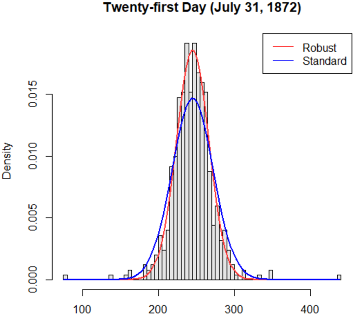
Step 1. For each day, we estimate the best-fitted Gaussian distribution ϕ t N p ˜ µ t , ˜ σ t q , where the parameters are robustly estimated: ˜ µ t is estimated by the median and ˜ σ t is estimated by dividing the interquartile range (IQR) by 1 . 349. The presence of large outlying observations makes the IQR-based robust-scale estimate more appropriate than the usual standard deviation based estimate of σ t ; see Fig. 2.
Step 2. For each experiment, compute the LP-coefficients between the assumed Φ t and the
18 Also, some misspecifications may be harmless as far as the final decision-making is concerned. Knowing the nature of deficiency can help us avoid over-complicating the model-0.
Figure 2: Two normal distributions are compared with different scale estimates: The red curve is based on the robust IQR-based scale estimate and the blue one is the usual standard deviation-based curve. Clearly, the blue curve underestimates the peak and overestimates the width of the density (due to the presence of few large values in the tails).
<details>
<summary>Image 2 Details</summary>
### Visual Description
\n
## Chart: Distribution Comparison - Robust vs. Standard (July 31, 1872)
### Overview
The image presents a comparative histogram showing the distribution of a dataset on July 31, 1872, using two different methods: "Robust" and "Standard". The chart displays density on the y-axis against values ranging from approximately 100 to 400 on the x-axis. Both distributions are visually similar, with a central peak around 250, but exhibit slight differences in their tails.
### Components/Axes
* **Title:** "Twenty-first Day (July 31, 1872)" - positioned at the top-center of the image.
* **X-axis:** Labeled implicitly by the range of values displayed (approximately 100 to 400). No explicit label is present.
* **Y-axis:** Labeled "Density" - positioned on the left side of the chart. The scale ranges from approximately 0.00 to 0.015.
* **Legend:** Located in the top-right corner.
* "Robust" - represented by a red line.
* "Standard" - represented by a blue line.
* **Data Representation:** Histograms with overlaid density curves. The histograms are composed of vertical bars of varying heights.
### Detailed Analysis
The chart shows two distributions.
**Robust (Red Line):**
The density curve for the Robust method initially rises from approximately x=150, reaches a peak density of approximately 0.013 at around x=250, and then declines, approaching zero around x=350. The histogram shows a concentration of data points around the peak, with fewer points at the extremes.
**Standard (Blue Line):**
The density curve for the Standard method also rises from approximately x=150, peaks at a density of approximately 0.012 at around x=250, and then declines, approaching zero around x=350. The histogram mirrors the Robust histogram in shape, with a similar concentration of data around the peak.
**Approximate Data Points (Extracted from visual estimation):**
| X-Value | Robust Density (approx.) | Standard Density (approx.) |
|---|---|---|
| 150 | 0.001 | 0.001 |
| 200 | 0.005 | 0.004 |
| 250 | 0.013 | 0.012 |
| 300 | 0.006 | 0.005 |
| 350 | 0.001 | 0.001 |
The Robust distribution appears to have slightly heavier tails than the Standard distribution, meaning it has a greater proportion of values further from the mean.
### Key Observations
* Both distributions are approximately symmetrical and unimodal (single peak).
* The peak of both distributions is located around x=250.
* The Robust distribution has a slightly wider spread and heavier tails compared to the Standard distribution.
* The difference between the two distributions is most noticeable in the tails.
### Interpretation
The chart compares two methods ("Robust" and "Standard") for estimating the distribution of a dataset. The fact that both methods produce similar distributions suggests that they are both reasonable approaches for this data. However, the slight differences in the tails indicate that the Robust method may be less sensitive to outliers or extreme values than the Standard method. This could be beneficial if the dataset contains errors or unusual observations. The title "Twenty-first Day (July 31, 1872)" suggests this data is part of a time series, and the comparison is being made on a specific date. Without further context, it's difficult to determine the nature of the data being analyzed, but the chart provides valuable insights into the distribution and potential differences between the two estimation methods. The data suggests a central tendency around 250, with a relatively narrow spread, indicating a consistent dataset.
</details>
empirical distribution r F t .
$$L P [ j ; \Phi _ { t } , \widetilde { F } _ { t } ] \ = \ \mathbb { E } \left [ T _ { j } ( X _ { t } ; \Phi _ { t } ) ; \widetilde { F } _ { t } \right ] \ = \ \frac { 1 } { n _ { t } } \sum _ { i = 1 } ^ { n _ { t } } T _ { j } ( x _ { t i } ; \Phi _ { t } ) .$$
for t 1 , 2 , . . . , 24 and j 1 , . . . , 4. The smoothed LP-coefficients (applying OPEN model selection method based on AIC-penalty; see equation 15) are stored in LP r t, j s : x LP r j ; Φ t , r F t s .
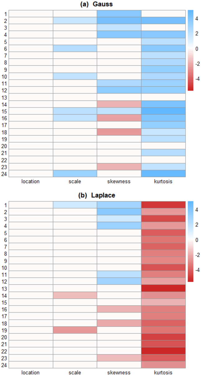
Step 3. LP-Map: Display the 24 4 LP-matrix as an image for easy visualization and interpretation. This is shown in Fig. 3(a).
Figure 3: Informative component analysis: LP-Map for Gauss and Laplace models. The rows denote different time points and columns are the order of LP coefficients LP r t, j s . This graphical explanatory method uncovers what are some of the most prominent ways a large number of related distributions differ from the anticipated f 0 p x q .
<details>
<summary>Image 3 Details</summary>
### Visual Description
## Heatmaps: Sensitivity Analysis of Statistical Parameters
### Overview
The image presents two heatmaps, labeled (a) Gauss and (b) Laplace, displaying a sensitivity analysis. Each heatmap visualizes the impact of four statistical parameters – location, scale, skewness, and kurtosis – on an unspecified metric, represented by the color intensity. The color scale ranges from -4 to 4, with red indicating negative values and blue indicating positive values. The y-axis represents values from 1 to 24.
### Components/Axes
* **Titles:** (a) Gauss, (b) Laplace
* **X-axis:** Labeled with "location", "scale", "skewness", and "kurtosis".
* **Y-axis:** Numbered from 1 to 24.
* **Color Scale:** Ranges from -4 (red) to 4 (blue), with 0 represented by white. The scale is positioned to the right of each heatmap.
* **Grid:** Both heatmaps are overlaid with a grid corresponding to the x and y-axis labels.
### Detailed Analysis or Content Details
**Heatmap (a) - Gauss**
* **Location:** Values are generally negative (red) for values 1-11, transitioning to positive (blue) for values 12-24. Approximate values: -3.5 at location 1, -2 at location 5, 0 at location 11, 2 at location 16, 3.5 at location 24.
* **Scale:** Values are predominantly positive (blue) for values 1-10, then become negative (red) for values 11-24. Approximate values: 3.5 at scale 1, 2 at scale 5, 0 at scale 11, -2 at scale 16, -3.5 at scale 24.
* **Skewness:** Values are mostly negative (red) for values 1-16, then become positive (blue) for values 17-24. Approximate values: -3.5 at skewness 1, -2 at skewness 5, 0 at skewness 16, 2 at skewness 20, 3.5 at skewness 24.
* **Kurtosis:** Values are generally positive (blue) for values 1-12, then become negative (red) for values 13-24. Approximate values: 3.5 at kurtosis 1, 2 at kurtosis 5, 0 at kurtosis 12, -2 at kurtosis 16, -3.5 at kurtosis 24.
**Heatmap (b) - Laplace**
* **Location:** Values are generally negative (red) for values 1-11, transitioning to positive (blue) for values 12-24. Approximate values: -3.5 at location 1, -2 at location 5, 0 at location 11, 2 at location 16, 3.5 at location 24.
* **Scale:** Values are predominantly positive (blue) for values 1-10, then become negative (red) for values 11-24. Approximate values: 3.5 at scale 1, 2 at scale 5, 0 at scale 11, -2 at scale 16, -3.5 at scale 24.
* **Skewness:** Values are mostly negative (red) for values 1-16, then become positive (blue) for values 17-24. Approximate values: -3.5 at skewness 1, -2 at skewness 5, 0 at skewness 16, 2 at skewness 20, 3.5 at skewness 24.
* **Kurtosis:** Values are generally positive (blue) for values 1-12, then become negative (red) for values 13-24. Approximate values: 3.5 at kurtosis 1, 2 at kurtosis 5, 0 at kurtosis 12, -2 at kurtosis 16, -3.5 at kurtosis 24.
### Key Observations
Both heatmaps (Gauss and Laplace) exhibit remarkably similar patterns. For each parameter (location, scale, skewness, kurtosis), there's a clear transition from negative to positive values around the midpoint of the y-axis (approximately values 11-17). This suggests a sensitivity point where the impact of the parameter changes sign. The magnitude of the values appears consistent across both distributions.
### Interpretation
These heatmaps likely represent a sensitivity analysis performed on a model or process that utilizes either a Gaussian (Normal) or Laplace distribution. The parameters being varied – location, scale, skewness, and kurtosis – are key characteristics defining the shape of these distributions.
The consistent patterns observed in both heatmaps suggest that the underlying model or process is similarly sensitive to changes in these parameters regardless of the chosen distribution (Gauss or Laplace). The transition points indicate that small changes in the parameter values around those points can lead to significant shifts in the model's output or behavior.
The fact that the color scale ranges from -4 to 4 suggests that the metric being measured is normalized or scaled in some way. Without knowing the specific metric, it's difficult to draw more concrete conclusions. However, the analysis reveals that the model is most sensitive to the parameters around the values 11-17 on the y-axis. This could be a critical region for parameter tuning or optimization.
</details>
Interpretation . What can we learn from the LP-map? It tells us the nature of non-Gaussianity of the error distributions for all 24 of the experiments in a compact way. The ICA-diagram detects three major directions of departure (from assumed Gaussian law) that more or less consistently appeared across different days of the experiment: (i) excess variability: This is indicated by the large positive values of the second-order LP-coefficients (2nd column of the LP-matrix) t LP t 2 u 1 / t / 24 . (ii) Asymmetry: It is interesting to note that the values of t LP t 3 u 1 / t / 24 change from positive to negative somewhere around the 15th day-which implies that the skewness of the distributions switches from left-skewed to right-skewed around the middle of the experiment. (iii) Long-taildness: Large positive values of t LP t 4 u 1 / t / 24 strongly indicate that the measurement densities are heavily leptokurtic, i.e., they possess larger tails than normal. These fatter tails generate large (or small) discrepant errors more frequently than expected-as we have witnessed in Fig. 1.
Laplace Error Distribution . Here we choose f 0 p x q as the Laplace p µ, s q distribution:
$$f _ { 0 } ( x ) = \frac { 1 } { 2 s } \exp \left ( - \frac { | x - \mu | } { s } \right ) , \, x \in \mathcal { R }$$
where µ P R and s ¡ 0. The unknown parameters are estimated using the maximum likelihood (MLE) method that automatically yields robust estimates: sample median for the location parameter µ and mean absolute deviation from the median for the scale parameter s .
The LP-map after applying the ICA algorithm is displayed in Fig. 3(b), which shows that a moderate degree of skewness and a major tail-repairing are needed to make Laplace consistent with the data. It is important to be aware of them to build a more realistic model of errorswhich is pursued in the next section.
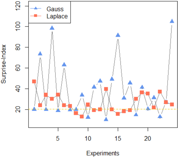
Laplace or Gauss? Following (14), compute
$$S I ( F _ { 0 t } , \widetilde { F } _ { t } ) \ = \ \sum _ { j = 1 } ^ { 4 } \left | \widehat { L P } [ t , j ] \, \right | ^ { 2 } ,$$
Figure 4: Shows the surprisal-indices (22) for the Gauss and Laplace models, over the sequence of 24 experiments. A 'small' value of SI p F 0 , r F q indicates that it is comparatively easier to repair f 0 p x q to fit the data. The plot provides a clear rational basis for choosing Laplace as a preferred model-0 since the blue curve consistently exceeds the orange curve for most experiments.
<details>
<summary>Image 4 Details</summary>
### Visual Description
## Line Chart: Surprise-Index vs. Experiments
### Overview
The image presents a line chart comparing the "Surprise-Index" for two distributions, "Gauss" (Gaussian) and "Laplace", across a series of "Experiments". The chart displays the Surprise-Index on the y-axis and the Experiment number on the x-axis. The Gauss distribution exhibits significantly higher and more variable Surprise-Index values compared to the Laplace distribution.
### Components/Axes
* **X-axis:** "Experiments" - ranging from approximately 1 to 23.
* **Y-axis:** "Surprise-Index" - ranging from approximately 0 to 120.
* **Data Series 1:** "Gauss" - represented by blue triangles (▲).
* **Data Series 2:** "Laplace" - represented by red squares (■).
* **Legend:** Located in the top-left corner, clearly labeling each data series with its corresponding symbol and name.
* **Horizontal dashed line:** A horizontal dashed line is present at approximately Surprise-Index = 20.
### Detailed Analysis
**Gauss (Blue Triangles):**
The Gauss line exhibits a highly oscillatory pattern. It starts at approximately 45 at Experiment 1, peaks at approximately 95 at Experiment 3, drops to approximately 15 at Experiment 4, then rises again to approximately 60 at Experiment 5. This pattern of peaks and troughs continues throughout the experiment series.
* Experiment 1: ~45
* Experiment 2: ~60
* Experiment 3: ~95
* Experiment 4: ~15
* Experiment 5: ~60
* Experiment 6: ~40
* Experiment 7: ~20
* Experiment 8: ~40
* Experiment 9: ~50
* Experiment 10: ~25
* Experiment 11: ~45
* Experiment 12: ~30
* Experiment 13: ~20
* Experiment 14: ~30
* Experiment 15: ~85
* Experiment 16: ~40
* Experiment 17: ~40
* Experiment 18: ~30
* Experiment 19: ~40
* Experiment 20: ~25
* Experiment 21: ~15
* Experiment 22: ~30
* Experiment 23: ~105
**Laplace (Red Squares):**
The Laplace line is relatively stable, fluctuating between approximately 20 and 40. It shows less pronounced peaks and troughs compared to the Gauss line.
* Experiment 1: ~30
* Experiment 2: ~35
* Experiment 3: ~30
* Experiment 4: ~20
* Experiment 5: ~35
* Experiment 6: ~30
* Experiment 7: ~25
* Experiment 8: ~30
* Experiment 9: ~35
* Experiment 10: ~25
* Experiment 11: ~30
* Experiment 12: ~30
* Experiment 13: ~20
* Experiment 14: ~25
* Experiment 15: ~35
* Experiment 16: ~30
* Experiment 17: ~30
* Experiment 18: ~30
* Experiment 19: ~35
* Experiment 20: ~25
* Experiment 21: ~20
* Experiment 22: ~30
* Experiment 23: ~35
### Key Observations
* The Gauss distribution consistently exhibits a higher Surprise-Index than the Laplace distribution.
* The Gauss distribution's Surprise-Index fluctuates dramatically, indicating a higher degree of unexpectedness or information content in each experiment.
* The Laplace distribution's Surprise-Index remains relatively stable, suggesting a more predictable outcome across experiments.
* The horizontal dashed line at Surprise-Index = 20 appears to serve as a baseline or threshold, with the Laplace distribution frequently hovering around this value.
### Interpretation
The chart suggests that the Gauss distribution generates more "surprising" outcomes compared to the Laplace distribution within the context of these experiments. The Surprise-Index, in this context, likely measures the degree to which the observed results deviate from expectations based on the respective distributions. The high variability in the Gauss distribution indicates that each experiment yields a relatively unpredictable result, while the Laplace distribution produces more consistent and expected outcomes. The horizontal line could represent a level of surprise considered "normal" or expected, and the Gauss distribution frequently exceeds this level, while the Laplace distribution often remains near or below it. This could imply that the Gauss distribution is better suited for scenarios where novelty or unexpected events are desired, while the Laplace distribution is more appropriate for situations requiring stability and predictability. The final peak in the Gauss distribution at Experiment 23 is particularly notable, suggesting a highly unexpected outcome at the end of the experiment series.
</details>
by taking the sum of squares of each row of the LP-matrix. Fig. 4 compares the surprisalindex for the normal and Laplace distribution over 24 experiments. From the plot, it is evident that Peirce's data were better represented by Laplace than by Gaussian.
## 5.2 Examples
The primary goal here is to show how density-sharpening provides a statistical method for repairing a scientifically meaningful model based on observed data. To that end, we apply the theory of density-sharpening to two specific day studies with f 0 p x q as the Laplace distribution.
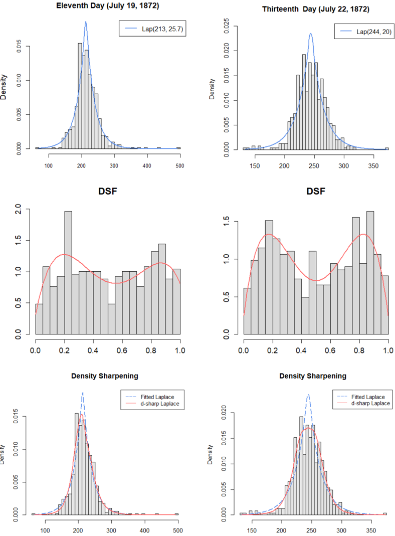
Study #11 (July 19, 1872). The best fitted Laplace distribution with mean 213 and scale parameter 25 . 7 is shown in the top left of Fig. 5. The estimated sharpening kernel with
Density
Figure 5: Mechanism of density-sharpening for 11th (1st column) and 13th (2nd column) day experiments. Top row: Display the best-fitted Laplace distributions f 0 . Middle row: Displays the estimate p d p u ; F 0 , r F q , which reveals the nature of statistical uncertainties of the Laplace models. Put it simply, the shape of p d p u ; F 0 , r F q answers the central question of discovery: What have we learned from the data that we did not already know? This helps to invent new hypotheses that are worthy of pursuit. Last row: Estimated SharpLaplace models f 0 p x q p d 0 p x q are shown (red curves). Here p d 0 p x q rectifies the shortcomings of Laplace model by 'bending' it in a data-adaptive manner.
<details>
<summary>Image 5 Details</summary>
### Visual Description
\n
## Histograms & Density Plots: Data Analysis from July 1872
### Overview
The image presents a 2x3 grid of plots, likely representing statistical analysis of data collected on the eleventh and thirteenth days of July 1872. Each pair of plots for a given day focuses on a different aspect of the data: a histogram with density curve, a Density Spectral Function (DSF) plot, and a Density Sharpening plot. The plots appear to be related to a distribution, potentially representing measurements or observations.
### Components/Axes
Each plot shares common elements:
* **X-axis:** Represents the data values. The scale varies between plots, ranging approximately from 0 to 500 in some and 150 to 350 in others.
* **Y-axis:** Labeled "Density" in the top row and unspecified in the middle and bottom rows, representing the probability density of the data. The scale ranges from 0 to approximately 0.025.
* **Titles:** Each plot has a title indicating the date and analysis type.
* **Histograms:** Represent the frequency distribution of the data, with bars indicating the count of observations within specific bins.
* **Density Curves:** Smooth curves overlaid on the histograms, representing the estimated probability density function.
* **DSF Plots:** Show a curve (red) and a histogram. The x-axis ranges from 0 to 1, and the y-axis ranges from 0 to 2.
* **Density Sharpening Plots:** Show two density curves (grey and light blue) overlaid on a histogram.
* **Laplace Parameters:** The top plots include "Lap(μ, σ)" notation, indicating a Laplace distribution fit to the data, with μ and σ representing the location and scale parameters, respectively.
### Detailed Analysis or Content Details
**Eleventh Day (July 19, 1872)**
* **Top-Left Plot:** Histogram and density curve. The distribution appears roughly unimodal, with a peak around 213. The Laplace parameters are Lap(213, 25.7). The density curve reaches a maximum density of approximately 0.014 at around 213.
* **Middle-Left Plot (DSF):** The red curve shows a peak around 0.2, with a value of approximately 1.6. The histogram is relatively flat, with values ranging from 0 to 1.5.
* **Bottom-Left Plot (Density Sharpening):** Two density curves are shown. The grey curve is smoother and has a peak around 213. The light blue curve is more jagged and has a similar peak.
**Thirteenth Day (July 22, 1872)**
* **Top-Right Plot:** Histogram and density curve. The distribution appears roughly unimodal, with a peak around 244. The Laplace parameters are Lap(244, 20). The density curve reaches a maximum density of approximately 0.022 at around 244.
* **Middle-Right Plot (DSF):** The red curve shows a peak around 0.4, with a value of approximately 1.5. The histogram is relatively flat, with values ranging from 0 to 1.5.
* **Bottom-Right Plot (Density Sharpening):** Two density curves are shown. The grey curve is smoother and has a peak around 244. The light blue curve is more jagged and has a similar peak.
### Key Observations
* The distributions on both days are unimodal and roughly symmetric.
* The peak of the distribution shifted from approximately 213 on July 19th to 244 on July 22nd.
* The scale parameter of the Laplace distribution decreased from 25.7 to 20, indicating a more concentrated distribution on July 22nd.
* The DSF plots show a similar pattern on both days, with a peak in the red curve.
* The Density Sharpening plots show two curves, one smoother and one more jagged, suggesting different methods of density estimation.
### Interpretation
The data suggests a change in the underlying distribution between July 19th and July 22nd. The shift in the peak and the decrease in the scale parameter indicate that the values are generally higher and more concentrated on July 22nd. The DSF plots may represent a spectral analysis of the data, highlighting specific frequencies or patterns. The Density Sharpening plots suggest that different methods of density estimation can produce slightly different results.
The Laplace distribution fitting suggests an attempt to model the data with a known distribution. The parameters (μ and σ) provide a concise summary of the distribution's location and spread. The DSF and Density Sharpening plots likely represent attempts to refine or analyze the density estimation further.
The consistent structure of the plots across both days suggests a systematic analysis of the data, potentially as part of a time series or longitudinal study. The specific meaning of the data would depend on the context in which it was collected.
</details>
smoothed LP-coefficients (see Sec. 4.2) is given below:
$$\begin{array} { r l } { d _ { 0 } ( x ) \, \colon = \, d ( F _ { 0 } ( x ) ; F _ { 0 } , F ) \, = \, 1 + 0 . 0 9 5 T _ { 3 } ( x ; F _ { 0 } ) - 0 . 1 4 8 T _ { 4 } ( x ; F _ { 0 } ) , } & { ( 2 3 ) \, d ( F _ { 0 } ( x ) ; F _ { 0 } , F ) \, = \, 1 + 0 . 0 9 5 T _ { 3 } ( x ; F _ { 0 } ) - 0 . 1 4 8 T _ { 4 } ( x ; F _ { 0 } ) , } \end{array}$$
and is shown in the middle panel.
The graphical display of d 0 p x q provides actionable insights into how to modify the Laplace distribution to reduce the empirical surprise. The non-zero x LP 3 and x LP 4 indicates that the Laplace distribution needs to be corrected for skewness and kurtosis, which is accomplished via LP-orthogonal series DS p F 0 , m q model (19):
$$\widehat { f } ( x ) \, = \, \frac { 1 } { 2 s _ { 0 } } \exp \left ( - \frac { | x - \mu _ { 0 } | } { s _ { 0 } } \right ) \, \left [ 1 \, + \, 0 . 0 9 5 T _ { 3 } ( x ; F _ { 0 } ) \, - \, 0 . 1 4 8 T _ { 4 } ( x ; F _ { 0 } ) \right ] ,$$
where p µ 0 , s 0 q p 213 , 25 . 7 q . The model (24) sharpens the assumed Laplace law to render it more closer to the observed fact. The bottom-left panel of Fig. 5 displays the asymmetric Laplace distribution with a shorter left-tail. The maxent DS p F 0 , m q estimate
$$\widehat { \widehat { f } } ( x ) = \frac { 1 } { 2 s _ { 0 } } \exp \left ( - \frac { | x - \mu _ { 0 } | } { s _ { 0 } } \right ) \, \exp \left \{ \, 0 . 0 9 8 T _ { 3 } ( x ; F _ { 0 } ) \, - \, 0 . 1 5 3 T _ { 4 } ( x ; F _ { 0 } ) \, - \, 0 . 0 1 5 2 \right \} ,$$
whose shape is almost indistinguishable from that of (24), and thus not displayed.
Study #13 (July 22, 1872). We apply the same steps to derive the error distributions of the day-13 experiment. We choose f 0 p x q as Laplace p 244 , 20 q and estimate the density-sharpening function:
$$d _ { 0 } ( x ) \, \colon = \, d ( F _ { 0 } ( x ) ; F _ { 0 } , F ) \, = \, 1 - 0 . 2 5 6 T _ { 4 } ( x ; F _ { 0 } ) .$$
The shape of p d 0 p x q clearly indicates that the peak and the tails of the initial Laplace distribution need repairing.
Ampliative character of our modeling: The DSF p d 0 p x q allows the Laplace to identify its own limitations and drives it to evolve into a new, more complete one:
$$\widehat { f } ( x ) \ = \ \frac { 1 } { 2 s _ { 0 } } \exp \left ( - \frac { | x - \mu _ { 0 } | } { s _ { 0 } } \right ) \, \left [ 1 \, - \, 0 . 2 5 6 T _ { 4 } ( x ; F _ { 0 } ) \right ] ,$$
with p µ 0 , s 0 q p 244 , 20 q ; shown in the bottom-right panel of Fig. 5. Compared with the Laplace distribution (the blue curve), the d -modified Laplace (the red curve) is much wider with a rounded peak and clipped tails.
## 6. A GENERALIZED LAW OF ERRORS
We have seen that for Peirce data, Laplace distribution was surprised in different manners for different experiments (refer Fig. 3b and Fig. 5): e.g., on day 11, the Laplace model got puzzled by the discrepancy in skewness, and tail of the measurement distribution, whereas on day 13, the surprise was mainly due to tail differences. The question naturally arises: how should a Laplace model respond to unexpected changes in data? A proposal for generalized law of errors is given that allows Laplace to automatically adapt to new data environments.
Definition 3 (Self-improving Laplace model) . We call X SharpLaplace ( m ), when the density of X obeys the following parameterizable form:
$$f ( x ) \ = \ \frac { 1 } { 2 s } \exp \left ( - \frac { | x - \mu | } { s } \right ) \, \exp \left \{ \sum _ { j = 1 } ^ { m } \theta _ { j } T _ { j } ( x ; F _ { 0 } ) \, - \, \Psi ( \pm b { \theta } ) \right \} , \quad x \in \mathcal { R } .$$
The insights gained from the analysis done in Sec. 5.2 suggest that m 4 or 6 could be perfectly reasonable for most practical purposes. The power of this model lies in its capacity to self-modify its structure in a data-driven manner.
Remark 13. SharpLaplace class of error models has inbuilt 'rules' (principles and mechanisms) that tell a Laplace how to adapt with the data in a completely autonomous fashion without being pre-programmed into them. This auto-adaptive nature makes this model realistic enough to be useful for a wide range of scientific applications.
## 7. PEIRCE'S LAW OF DISCOVERY
Not the smallest advance can be made in knowledge beyond the stage of vacant staring, without making an abduction at every step. - C. S. Peirce (1901)
All empirical scientific inquiry goes through three fundamental inferential phases:
- Discovery: developing new testworthy hypotheses;
- Hypothesis testing: confirming the plausibility of a hypothesis;
- Prediction: predicting by extrapolating the acceptable model.
Over the last century or so, statistical inference has been dominated by hypothesis testing and prediction 19 problems, virtually neglecting the key question of where the reasonable hypothesis came from, leaving it to the scientists' imagination and speculation. In the article 'Statistics for Discovery,' George E. P. Box argued that
[S]tatistics has been overly influenced by mathematical methods rather than the scientific method and consequently the subject has been greatly skewed towards testing rather than discovery. - George Box (2001)
Our focal interest is in the problem of discovery, not confirmation or prediction. We showed how density-sharpening based modeling can provide the basis for developing statistical laws of discovery.
Charles Sanders Peirce introduced the idea of abductive inference (as opposed to inductive inference) to describe the process of generating hypotheses in order to explain surprising facts. He developed abductive reasoning over 50 years (between 1865 and 1914), and it is considered as Peirce's most significant contribution to the logic of science. According to Peirce, abduction 'is the only logical operation which introduces any new idea.' The importance of abduction for scientific discovery was further stressed by Heckman and Singer (2017):
19 Discovery is much harder than prediction because one can go away with good prediction without understanding. But for discovery, understanding 'how and why' is a must.
Abduction is different from falsification or corroboration. It moves descriptions of the world forward rather than just confirming or falsifying hypotheses. It is part of a process of discovery where model reformulation, revision of hypotheses and addition of new information are part of the process.
Abductive Inference Machine (AIM) . This paper lays out a proposal for algorithmic operationalization of Peircean style abductive inference and discovery. In particular, we described how the density-sharpening principle can help us design an Abductive Inference Machine ( AIM 20 ) that (i) allows us to properly handle model uncertainty and misspecifications; (ii) produces abductive instinct -by guiding us to make better decisions (than depending on pure luck alone) in formulating and adopting new promising hypotheses that have a better chance of being true; and (iii) generates a preferred course of actions for extracting statistical models from experimental data by revising an initially misspecified scientific model.
## 8. AIM: SCIENCE OF MODEL DEVELOPMENT AND REVISION
AIM is a theory of model-revision , not parameter estimation (MLE/Bayes/robust methods) or curve-fitting (machine learning methods). There are some unique objectives and challenges, which set it apart from traditional data modeling cultures. In the following, we will highlight a few major ones (D1-D7), taking help from the Peirce data analysis done in Section 5.
Four stages of abductive model building:
1. Initial state. AIM starts with an approximate model f 0 (based on, say, some economic theory) and measurements. 21 The top left density in Fig. 5 shows the best-fitted theoretical model-the Laplace distribution for experiment #11, where the unknown parameters were estimated using MLE.
D1 Non-standard inferential questions: Justification discovery . However, for modern econometricians and policymakers, parameter estimation or significance testing routines (clas-
20 It tells empirical analysts where to AIM as they search for possible new discoveries.
21 In our context, the theory of Laplace's law of error was confronted with Peirce's experimental data.
sical inference; see Haavelmo (1944)) are not the most interesting issues. Modern quantitative economists are more concerned with questions like: 'How far is our speculated model from reality? What are the most important gaps in our understanding? In which directions can I improve my theory-based model?' Developing a general approach to answering these modeling questions is the central imperative of AIM .
2. Encountering surprise . 'Surprise' jumpstarts the abductive learning process. Surprise essentially means that there is something new in the data relative to the assumed model f 0 , which we estimate by SI p F 0 , F q following Eq. (14). Simply put, it quantifies how much new information is left on the data to be explained; see the orange curve in Fig. 4. Intelligent learners (agents) utilize surprise as a source of additional information to learn something new about the phenomena.
D2 Model-disequilibrium theory . A 'large' value of SI p F 0 , F q indicates the model is 'out of equilibrium' with the current environment, and to restore equilibrium, a careful revision of the current theoretical model (beyond parameter tuning) is necessary. But how do we sharpen the existing model? Can we develop an automatic procedure to generate the sharpening rules? These questions are beyond the reach of classical statistical learning methods. AIM approaches these questions by first characterizing the 'knowledge-gap' between the postulated theory and the observed measurements.
3. Discovering the knowledge-gap . Fig. 5 (left of middle panel) displays the estimated sharpening kernel p d p u ; F 0 , F q for experiment #11, which acts as a 'channel' through which information flows from the data to the model-obeying the density-sharpening principleto bring the system (model-data) back to equilibrium. Accordingly, p d p u ; F 0 , F q acts as a 'bridge' between a theorized model and actual measurements. The following remark by Trygve Haavelmo (1944) highlights how crucial this accomplishment is:
The method of econometric research aims, essentially, at a conjunction of economic theory and actual measurements, using the theory and technique of statistical inference as a bridge pier.
D3 Hypotheses generation . Abduction is the logic of discovery. Why do we need a logic for discovery? Charles Peirce, Herbert Simon, and many other prolific researchers believed that a trial-and-error search for 'invention' is seldom a worthwhile strategy, especially for complex systems (like economics, biology, etc.). Norwood Hanson said it beautifully in his book:
' If establishing an hypothesis through its predictions has a logic, so has the conceiving of an hypothesis. ' -Patterns of Discovery
(1958)
AIM helps scientists to make educated guesses-on what's the next best hypothesis to try from a vast pool of conceivable collections-by autonomously learning new realities from the data through d 0 p x q . Classical inference, on the other hand, mainly deals with the confirmatory or predictive side of data analysis, not hypotheses generation and discovery.
D4 Modeling surprise, not the full data . AIM searches for patterns in the 'unexplained rest'-the parts of the data that were left unexplained by the existing theory. Notice that we are not blindly searching for patterns in the full data; we are only focusing on the novel parts of the data that contain new information. It is important to distinguish between these two aspects. Our goal is to accelerate discovery by synthesizing a simple explanatory model p d p u ; F 0 , F q for the surprising phenomena.
D5 Information-filtering unit . The density-sharpening kernel acts as a filter that discards redundant information and compactly summarizes the new information (knowledge-gap) as a probability density function. 22 The non-zero LP-coefficients of p d p u ; F 0 , F q identify the missing elements of reality in the current theoretical model. For example, Eq. 23 implies that the Laplace law is misspecified in terms of symmetry (3rd order) and long-tailedness (4th order); also check the 11th row of the LP-map shown in Fig. 3. Standard statistical learning methods don't have any such capabilities.
22 As Herbert Simon said: 'Anything that gives us new knowledge gives us an opportunity to be more rational.' From that perspective, AIM could be a powerful tool to guide economic agents in making rational decisions under uncertainty. More details can be found in Mukhopadhyay (2022b).
4. Model-editing . AIM fills the knowledge-gaps by revising initial probability model based on the principle of density-sharpening, which can be described by a simple logical formula:
<details>
<summary>Image 6 Details</summary>

### Visual Description
Icon/Small Image (919x57)
</details>
Every successive iteration of the above procedure generates a more realistic model than its predecessors. Here the density-sharpening kernel d 0 p x q represents the progress in our understanding, which makes the hypothesized simplified model elastic enough to be adaptable for real-data. 23
By executing (29), AIM designs a class of most pursuitworthy alternative models for the data and selects the best one using the 'law of lazy update.' 24 Eq. 25 shows the sharp-Laplace model for study #11, also displayed in the bottom of Fig. 5. The parsimonious d 0 p x q keeps the final model 'sophisticatedly simple' 25 by smoothly extending the hypothesized Laplace model to explain the data.
D6 AIM Curve-fitting . One of the non-standard aspects of AIM is that it's not about building fancy empirical models starting from a clean slate-it's about building a statistical structure on top of the already existing scientific knowledge base to advance the current theory. 26 In doing so, it provides efficient ways of handling an idealized simple model for discovering new knowledge from complex real-world data.
D7 Conservative-liberal coalition . Note that the derived sharp-probabilistic law (e.g., eq. 25) combines the generality (generic features) of Laplace's laws of error with the specificity (stylized features) of Peirce's data. This coalition of conservative (sticking to current dogma) and liberal (openness to course correction when necessary) ideologies makes our data modeling philosophy stands out from traditional statistical and machine learning data-fitting methods.
23 In other words, we don't believe in the 'one-fits-all' model. Our goal is to provide economists with a systemic principle for iteratively revising their preliminary models by confronting them with real-world data.
24 It is fundamentally different from model selection or multiple hypothesis testing, which deals with a pre-determined set of alternative models. Model discovery and model selection are two very different things.
25 Arnold Zellner (2007): 'a much heavier emphasis on sophisticated simplicity in econometrics is needed.' 26 In more simple terms, AIM = Learning from data by standing on the foundation of existing knowledge.
## 9. AI = ABDUCTIVE INTELLIGENCE
When can we say a model is behaving intelligently? This is no easy question. However, at least part of the answer, I believe, lies in inspecting how the model reacts to surprise and adapts to changes. An intelligent model should not be 'brittle,' which collapses all of a sudden upon encountering surprises from the data. The model should have an 'internal' mechanism that help it rise to the occasion by providing recommendations for how to put together incomplete pre-existing knowledge (encoded in model-0) with the data. We refer to this core intellectual component of any learning problem as 'abductive intelligence.'
Building models that are capable of improving themselves has been a dream of computer scientists since the inception of the artificial intelligence field in 1956. It was at the top of the agenda in the proposal written for the Dartmouth Summer Research Project on artificial intelligence:
' Probably a truly intelligent machine will carry out activities which may best be described as self-improvement. ' -John McCarthy et al. (1955)
More than developing new ways of building data models, we need new principles for sharpening an existing model's infrastructure. Such a model, equipped with self-improving capability, then gradually acquires more knowledge about the environment by building increasingly refined models of reality.
'Once we have devised programs with a genuine capacity for self-improvement a rapid evolutionary process will begin. As the machine improves both itself and its model of itself, we shall begin to see all the phenomena associated with the terms 'consciousness,' 'intuition' and 'intelligence' itself.' -Marvin Minsky (1966)
Remark 14 (Intelligence of a Model) . A model's 'intelligence' is its capacity to change and remodel itself when confronted with new data. Any model which is not capable of 'selfimproving' is a disposable, dead model.
Remark 15 (Designing an Intelligent Model) . Model is a work in progress; there is no such thing as the 'final model.' The important part is knowing how to expand the knowledge base by sharpening yesterday's version. With that being said, the focus of present-day machine learning has primarily been on developing a good subordinate-model f 0 p x q but not so much on designing the supervisory-model d 0 p x q . To achieve the goal of designing intelligent machines, it seems inevitable that we have to shift our attention to the 'supervisory' part of the modelthat which knows how to react to surprise in order to evolve to its next avatar. In the long run, the durability of a model depends more on its skill to adapt than its built-in skill . And to design such self-improving models, we will need to instill 'abductive intelligence' in the existing machine learning systems-which is the goal of AIM .
## 10. PEIRCE: AN EXPLORER UPON UNTRODDEN GROUND
I was an explorer upon untrodden ground - C. S. Peirce (1902)
Bertrand Russell (1959) described Charles Sanders Peirce as 'one of the most original minds of the later nineteenth century, and certainly the greatest American thinker ever.' He was a craftsman of the highest order, who made some eminent contributions to the development of nineteenth-century American Statistics. Peirce analyzed his 1872 experimental data in the paper 'On the theory of errors of observation'-which is a gold mine of ideas. His techniques and philosophy of data analysis reported in the paper were a testament to his brilliance as a master applied statistician. On the landmark occasion of 150th anniversary of his famous 1872 study, 27 we have looked back at his views on empirical modeling. The current article offers a framework that embraces and operationalizes the Peircean view of discovery and statistical modeling. We called this framework AIM -Abductive Inference Machine-which is grounded in the principle of density sharpening and a new class of models called 'dyadic models.' We
27 A miraculous year: In 1872, exactly the same year of Peirce's experiment, Ludwig Boltzmann established the probabilistic (statistical) foundation of the entropy function-the birth of modern information theory. As we have seen in this article, Peircean abduction and information theory are intimately connected through the concept of density-sharpening. As a matter of fact, AIM stands on three pillars: Abductive inference + information theory + density-sharpening law.
have illustrated the key algorithmic steps and philosophical aspects of our modeling approach using Peirce's 1872 experimental data to reveal new insights on the probabilistic nature of measurement uncertainties.
## STATEMENTS AND DECLARATIONS
The Author declares that there is no conflict of interest/competing interests.
## ACKNOWLEDGEMENT
The author was benefited from conversations and/or correspondence with James Heckman, Burton Singer, and Stephen Stigler. We also thank the editorial board for their thoughtful and philosophical comments on the manuscript.
2022 marks the 150th anniversary of C. S. Peirce's historic experiment-which according to Stigler (1978) is one of the most significant statistical investigations in the history of nineteenth-century American mathematical research. This paper celebrates this landmark occasion by introducing a modern approach to Peircean abduction, which is readily applicable in practice.
## REFERENCES
- Bailey, D. C. (2017). Not normal: the uncertainties of scientific measurements. Royal Society open science 4 (1), 160600.
- Box, G. (2001). Statistics for discovery. Journal of Applied Statistics 28 (3-4), 285-299.
- Box, G. E. (1976). Science and Statistics. Journal of the American Statistical Association 71 (356), 791-799.
- Buansing, T. T., A. Golan, and A. Ullah (2020). An information-theoretic approach for forecasting interval-valued sp500 daily returns. International Journal of Forecasting 36 (3), 800-813.
- Burch, R. and K. A. Parker (2022). Charles Sanders Peirce. In E. N. Zalta (Ed.), The Stanford Encyclopedia of Philosophy (Summer 2022 ed.). Stanford University.
- Crease, R. P. (2009). Charles Sanders Peirce and the first absolute measurement standard. Physics Today 62 (12), 39.
- Golan, A. (2018). Foundations of info-metrics: Modeling, inference, and imperfect information . Oxford University Press.
- Haavelmo, T. (1944). The probability approach in econometrics. Econometrica: Journal of the Econometric Society , iii-115.
- Hanson, N. R. (1965). Patterns of discovery: An inquiry into the conceptual foundations of science . CUP Archive.
- Heckman, J. J. and B. Singer (2017). Abducting economics. American Economic Review 107 (5), 298-302.
- Jaynes, E. T. (1957). Information theory and statistical mechanics. Physical review 106 (4), 620.
- Laplace, P. S. (1774). M´ emoire sur la probabilit´ e de causes par les ´ evenements. M´ emoire de l'acad´ emie royale des sciences .
- Lee, T.-H., M. Y. Mao, and A. Ullah (2021). Maximum entropy analysis of consumption-based capital asset pricing model and volatility. Journal of Econometric Methods 10 (1), 1-19.
- Maasoumi, E. (1993). A compendium to information theory in economics and econometrics. Econometric reviews 12 (2), 137-181.
- Mao, Y., A. Ullah, et al. (2020). Information theoretic estimation of econometric functions. Forthcoming in Advances in Info-Metrics: Information and Information Processing across Disciplines .
- McCarthy, J., M. L. Minsky, N. Rochester, and C. E. Shannon (1955). A proposal for the Dartmouth Summer Research Project on Artificial Intelligence. Online: http://wwwformal.stanford.edu/jmc/history/dartmouth.pdf.
- Minsky, M. (1966). Artificial intelligence. Scientific American, 215 (3), 257.
- Mukhopadhyay, S. (2017). Large-scale mode identification and data-driven sciences. Electronic Journal of Statistics 11 (1), 215-240.
- Mukhopadhyay, S. (2022a). A maximum entropy copula model for mixed data: Representation, estimation, and applications. in press, arXiv:2203.03040 , 1-35.
- Mukhopadhyay, S. (2022b). Modelplasticity and abductive decision making. Technical Report, arXiv:2203.03040 , 1-27.
- Mukhopadhyay, S. and D. Fletcher (2018). Generalized empirical Bayes modeling via frequentist goodness-of-fit. Nature: Scientific Reports 8 (9983), 1-15.
- Mukhopadhyay, S. and E. Parzen (2020). Nonparametric universal copula modeling. Applied Stochastic Models in Business and Industry, special issue on 'Data Science' 36 (1), 77-94.
- Parkes, D. C. and M. P. Wellman (2015). Economic reasoning and artificial intelligence. Science 349 (6245), 267-272.
- Peirce, C. (1902). Minute logic, Chapter I. Intended characters of this treatise. Digital Companion to CS Peirce .
- Peirce, C. S. (1873). On the theory of errors of observation. Report of the Superintendent of the U.S. Coast Survey , 200-224.
- Peirce, C. S. (1901). The proper treatment of hypotheses: A preliminary chapter, toward an examination of hume's argument against miracles, in its logic and in its history. MS 692 , 890-904.
- Peirce, C. S. (1931-58). The collected papers of Charles Sanders Peirce, eds. C Hartshorne, P Weiss (vols. 1-6) and A Burks (vols. 7-8), Cambridge, MA: Harvard University Press, 1931-58 and 1960-66 .
- Peirce, C. S. (2009). Writings of Charles S. Peirce: a chronological edition, volume 3: 18721878 , Volume 3. Indiana University Press.
- Rao, C. R. (2001). Statistics: Reflections on the past and visions for the future. Communications in Statistics-Theory and Methods 30 (11), 2235-2257.
- Russell, B. (1959). Wisdom of the West, a Historical Survey of Western Philosophy in Its Social and Political Setting . Garden City, NY: Doubleday.
- Simon, H. A. (1988). The science of design: Creating the artificial. Design Issues , 67-82.
- Stigler, S. M. (1978). Mathematical statistics in the early states. The Annals of Statistics , 239-265.
- Tukey, J. W. (1969). Analyzing data: Sanctification or detective work? American Psychologist 24 (2), 83.
- Tukey, J. W. (1972). Exploratory data analysis: As part of a larger whole. In Proceedings of the 18th conference on design of experiments in Army research and development I. Washington, DC , Volume 1010.
- Tukey, J. W. (1977). Exploratory data analysis , Volume 2. Reading, Mass.
- Wilson, E. B. and M. M. Hilferty (1929). Note on C. S. Peirce's experimental discussion of the law of errors. Proceedings of the National Academy of Sciences of the United States of America 15 (2), 120.
- Zellner, A. (2007). Philosophy and objectives of econometrics. Journal of Econometrics 136 (2), 331-339.