2111.08404

## Practical Timing Side Channel Attacks on Memory Compression Martin Schwarzl Graz University of Technology martin.schwarzl@iaik.tugraz.at Pietro Borrello Sapienza University of Rome borrello@diag.uniroma1.it Michael Schwarz CISPA Helmholtz Center for Information Security michael.schwarz@cispa.saarland Abstract -Compression algorithms are widely used as they save memory without losing data. However, elimination of redundant symbols and sequences in data leads to a compression side channel. So far, compression attacks have only focused on the compression-ratio side channel, i.e. , the size of compressed data, and largely targeted HTTP traffic and website content. In this paper, we present the first memory compression attacks exploiting timing side channels in compression algorithms, targeting a broad set of applications using compression. Our work systematically analyzes different compression algorithms and demonstrates timing leakage in each. We present Comprezzor, an evolutionary fuzzer which finds memory layouts that lead to amplified latency differences for decompression and therefore enable remote attacks. We demonstrate a remote covert channel exploiting small local timing differences transmitting on average 643 . 25bit ♥ h over 14 hops over the internet. We also demonstrate memory compression attacks that can leak secrets bytewise as well as in dictionary attacks in three different case studies. First, we show that an attacker can disclose secrets co-located and compressed with attacker data in PHP applications using Memcached. Second, we present an attack that leaks database records from PostgreSQL, managed by a Python-Flask application, over the internet. Third, we demonstrate an attack that leaks secrets from transparently compressed pages with ZRAM, the memory compression module in Linux. We conclude that memory-compression attacks are a practical threat. ## I. INTRODUCTION Data compression plays a vital role for performance and efficiency. For example, compression leads to smaller data footprints, allowing more data to be stored in memory. Memory accesses are typically faster than retrieving data from slower mediums such as hard disks or solid-state disks. As a result, both Microsoft [63] and Apple [3] rely on memory compression in their operating systems (OSs) to better utilize memory. Similarly, memory compression is also used in databases [46] or keyvalue stores [45]. Compression can also increase performance when storing or transferring data on slow mediums. Hence, data compression is also widely used for HTTP traffic [41], [15] and file-system compression [6]. While compression has many advantages, it is problematic in scenarios where sensitive data is compressed [49], [20], [4], [58], [57], [32]. Attacks such as CRIME [49], BREACH [20], Gururaj Saileshwar Georgia Tech Graz University of Technology gururaj.s@gatech.edu Hanna M¨ uller Graz University of Technology h.mueller@student.tugraz.at Daniel Gruss Graz University of Technology daniel.gruss@iaik.tugraz.at TIME [4], or HEIST [58], exploit the combination of encryption and compression in TLS-encrypted HTTP traffic. Karaskostas et al. [32] extended BREACH to commonly used ciphers, such as AES. These attacks demonstrated that an attacker could learn secrets when they are compressed together with attacker-controlled input. However, all these attacks focused on web traffic and only exploited differences in the compressed size of data. The size of compressed data is either accessed directly [49], e.g., in a man-in-the-middle (MITM) attack or indirectly by observing the impact of the compressed size on the transmission time [4]. Although attacks exploiting the compression ratio were first described by Kelsey et al. [33] in 2002, most attacks thus far have focused on compressed web traffic. Surprisingly, security implications of compression in other settings, such as virtual memory and file systems, have not been studied thoroughly. Also, compression fundamentally provides a reduction in size of data at the expense of additional time required for compression and decompression. However, so far, only the result of the compression, i.e. , the compressed size, has been exploited to leak data but not the time consumed by the process of compression or decompression itself. In this paper, we demonstrate that the decompression time also leaks information about the compressed data. Instead of focussing on the final compressed data, we measure the time it takes to decompress data. Hence, we do not need to observe the transport of the compressed data. Decompression timing can be measured in several scenarios, e.g., a simple read access to the data can suffice for compressed virtual memory or file systems. Moreover, decompression timings can be observed remotely, even when the compressed data never leaves the victim system. We systematically analyzed six compression algorithms, including widely-used algorithms such as DEFLATE (in zlib), PGLZ (in PostgreSQL), and zstd (by Facebook). We observe that the decompression time not only correlates with the entropy of the uncompressed data, but also with various other aspects, such as the relative position or alignment of compressible data. In general, these timing differences arise due to the design of the compression algorithm and its implementation. To explore these parameters in an automated fashion, we introduce Comprezzor, an evolutional fuzzer. In line with previous attacks on compression, Comprezzor assumes that parts of the compressed data are controlled by an attacker. Based on this assumption and a target secret, Comprezzor searches for a memory layout that maximizes the timing differences for decompression timing attacks. As a result, Comprezzor discovers a memory layout for compression algorithms which leads to decompression timing attacks with high-latency differences up to three orders of magnitude higher than manually discovered layouts. Based on the results of Comprezzor, we present three case studies demonstrating that these timing differences can be exploited in realistic scenarios to leak sensitive data. We demonstrate that these timing differences can be exploited even in remote attacks on an in-memory database system without executing code on the victim machine and without observing the victim's network traffic. Hence, our case studies show that compressing sensitive data poses a security risk in any scenario using compression and not just for web traffic. In the first case study, we build a remote covert channel which works across 14 hops on the internet, abusing the memory compression of Memcached, an in-memory object caching system. By measuring the execution time of a public PHP API of an application using Memcached, we can covertly transfer data between two computers at an average transmission rate of 643 . 25 bit ♥ h with an error rate of only 0 . 93 % . In a similar setup, we also demonstrate the capability of leaking a secret bytewise co-located with data compressed by a PHP application into Memcached, in 31 . 95 min ( n 20 , σ 8 . 48% ) over the internet. Using a dictionary with 100 guesses, we leak a 6 B -secret in 14 . 99 min . In the second case study, we exploit the transparent database compression of PostgreSQL. Our exploit leaks database records from an inaccessible database table of a remote web app. We show that as long as an attacker can co-locate data with a secret, it is possible for the attacker to influence and observe decompression times when accessing the data, thus, leaking secret data. Such a scenario might arise if structured data, i.e. , JSON documents, are stored with attack-controlled fields into a single cell. Using an attack that leaks a secret bytewise, we leak a 6 B -secret in 7 . 85 min . Our dictionary attack runs in 8 . 28 min on average over the internet for 100 guesses. In the third case study, we exploit ZRAM, the memory compression module in Linux. We demonstrate that even if the application itself or the file system does not compress data, the OS's memory compression can transparently introduce timing side channels. We demonstrate that a dictionary attack with 100 guesses on ZRAM decompression can leak a 6 B -secret co-located with attacker data in a page within 2 . 25 min on average. Our fuzzer shows that most if not all compression algorithms are susceptible to timing side channels when observing the decompression of data. With our case studies, we demonstrate that data leakage is not only a concern for data in transit but also for data at rest. With this work, we seek to highlight the importance of evaluating the trade-off between compressing data, and leaking side-channel information about the compressed data, for any system adopting compression. Contributions. 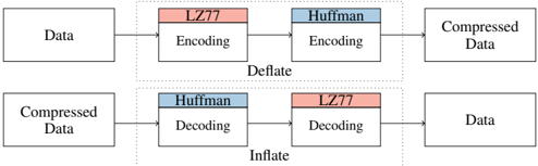The main contributions of this work are: Fig. 1: DEFLATE algorithm has two parts: LZ77 part to compress sequences and a Huffman part to compress symbols. <details> <summary>Image 1 Details</summary>  ### Visual Description \n ## Diagram: Deflate/Inflate Process ### Overview The image is a diagram illustrating the Deflate and Inflate processes, which are used for data compression and decompression respectively. It shows a two-stage process involving LZ77 and Huffman encoding/decoding. The diagram depicts a flow from "Data" to "Compressed Data" via Deflate, and from "Compressed Data" back to "Data" via Inflate. ### Components/Axes The diagram consists of rectangular blocks representing processing stages, connected by arrows indicating the flow of data. The key components are: * **Data:** The initial input. * **Compressed Data:** The output after compression. * **LZ77 Encoding:** A compression algorithm. The block is colored light red. * **Huffman Encoding:** Another compression algorithm. The block is colored light blue. * **LZ77 Decoding:** The decompression counterpart of LZ77 Encoding. The block is colored light red. * **Huffman Decoding:** The decompression counterpart of Huffman Encoding. The block is colored light blue. * **Deflate:** A label encompassing the LZ77 Encoding and Huffman Encoding stages. * **Inflate:** A label encompassing the Huffman Decoding and LZ77 Decoding stages. The arrows indicate the direction of data flow. ### Detailed Analysis or Content Details The diagram shows two parallel processes: **Deflate (Compression):** 1. Data flows from left to right. 2. First, it enters the "LZ77 Encoding" block (light red). 3. The output of LZ77 Encoding then flows into the "Huffman Encoding" block (light blue). 4. Finally, the output of Huffman Encoding results in "Compressed Data". **Inflate (Decompression):** 1. "Compressed Data" flows from right to left. 2. First, it enters the "Huffman Decoding" block (light blue). 3. The output of Huffman Decoding then flows into the "LZ77 Decoding" block (light red). 4. Finally, the output of LZ77 Decoding results in "Data". The diagram does not contain any numerical data or specific values. It is a conceptual representation of the process. ### Key Observations The diagram highlights that Deflate uses a two-stage compression process, and Inflate reverses this process for decompression. The order of operations is crucial: LZ77 is applied before Huffman in compression, and Huffman is applied before LZ77 in decompression. The color coding (red for LZ77, blue for Huffman) is consistent throughout the diagram, aiding in understanding the flow. ### Interpretation The diagram illustrates a common data compression technique. Deflate, as shown, combines the strengths of two different compression algorithms. LZ77 is effective at removing redundant sequences of data, while Huffman coding efficiently represents frequently occurring symbols with shorter codes. By combining these, Deflate achieves a good compression ratio. The Inflate process simply reverses these steps to recover the original data. This diagram is a high-level overview and doesn't delve into the specifics of how each algorithm works internally. It focuses on the overall flow and the relationship between the components. The diagram suggests a reversible process, meaning no data is lost during compression and decompression. </details> - 1) We present a systematic analysis of timing leakage for several lossless data-compression algorithms. - 2) We demonstrate an evolutional fuzzer to automatically search for memory layouts causing large timing differences for timing side channels on memory compression. - 3) We show a remote covert channel exploiting the in-memory compression of PHP-Memcached. - 4) We demonstrate that compression-based timing side channels can be introduced by compression in applications, databases, or the system's memory compression. - 5) We leak secrets from Memcached, PostgreSQL, and ZRAM within minutes. Outline. In Section II, we provide background. In Section III, we present attack model and building blocks. In Section IV, we systematically analyze compression algorithms. In Section V, we present Comprezzor. In Section VI, we demonstrate local and remote attacks exploiting decompression timing. We discuss mitigations in Section VII and conclude in Section VIII. We responsibly disclosed our findings to the developers and will open-source our fuzzing tool and attacks on Github. ## II. BACKGROUND AND RELATED WORK In this section, we provide background on data compression algorithms, prior side-channel attacks on data compression, and the use of fuzzing to discover side channels. ## A. Data Compression Algorithms Lossless compression reduces the size of data without losing information. One of the most popular algorithms is the DEFLATE compression algorithm, which is used in gzip (zlib). The DEFLATE compression algorithm [12] consists of two main parts, LZ77 and Huffman encoding and decoding, as shown in Figure 1. The Lempel-Ziv (LZ77) part scans for the longest repeating sequence within a sliding window and replaces repeated sequences with a reference to the first occurrence [8]. This reference stores distance and length of the occurrence. The Huffman -coding part tries to reduce the redundancy of symbols. When compressing data, DEFLATE first performs LZ77 encoding and Huffman encoding [8]. When decompressing data (inflate), they are performed in reverse order. The algorithm provides different compression levels to optimize for compression speed or compression ratio. The smallest possible sequence has a length of 3 B [12]. Other algorithms provide different design points for compressibility and speed. Zstd, designed by Facebook [10] for modern CPUs, improves both compression ratio and speed, and is used for compression in file systems (e.g., btrfs, squashfs) and databases (e.g., AWS Redshift, RocksDB). LZ4 and LZO are other algorithms used in file systems, which are optimized for compression and decompression speed. LZ4, in particular, gains its performance by using a sequence compression stage (LZ77) without the symbol encoding stage (Huffman) like in DEFLATE. FastLZ, similar to LZ4, is a fast compression algorithm implementing LZ77. PGLZ is a fast LZ-family compression algorithm used in PostgreSQL for varying-length data in the database [46]. ## B. Prior Data Compression Attacks In 2002, Kelsey [33] first showed that any compression algorithm is susceptible to information leakage based on the compression-ratio side channel. Duong and Rizzo [49] applied this idea to steal web cookies with the CRIME attack by exploiting TLS compression. In the CRIME attack, the attacker adds additional sequences in the HTTP request, which act as guesses for possible cookies values, and observes the request packet length, i.e. , the compression ratio of the HTTP header injected by the browser. If the guess is correct, the LZ77-part in gzip compresses the sequence, making the compression ratio higher, thus allowing the secret to be discovered. To perform CRIME, the attacker needs to be able to spy on the packet length, and the secret needs to have a known prefix such as sessionid= or cookie= . To mitigate CRIME, TLS-level compression was disabled for requests [4], [20]. The BREACH attack [20] revived the CRIME attack by attacking HTTP responses instead of requests and leaking secrets in the HTTP responses such as cross-site-request-forgery tokens. The TIME attack [4] uses the time of a response as a proxy for the compression ratio, as it can be measured even via JavaScript. To reliably amplify the signal, the attacker chooses the size of the payload such that additional bytes, due to changes in compressibility, cross a boundary and cause significantly higher delays in the round-trip time (RTT). TIME exploits the compression ratio to amplify timing differences via TCP windows and does not exploit timing differences in the underlying compression algorithm itself. A malicious site can perform a TIME attack on their visitors to break same-origin policy or leak data from sites that reflect user input in the response, such as a search engine [4]. Vanhoef and Van Goethem [58] showed with HEIST that HTTP/2 features can also be used to determine the size of crossorigin responses and to exploit BREACH using the information. Van Goethem et al. [57] similarly showed that compression can be exploited to determine the exact size of any resource in browsers. Karaskostas and Zindros[32] presented Rupture, extending BREACH attacks to web apps using block ciphers such as AES. Tsai et al. [55] demonstrated cache timing attacks on compressed caches, which can leak a secret key in under 10 ms . Common Theme. All of the prior attacks primarily exploit the compression-ratio side channel. However, the time taken by the underlying compression algorithm for compression or decompression is not analyzed or exploited as side channels. 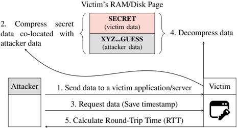Additionally, these attacks largely target the HTTP traffic and website content, and do not focus on the broader applications Fig. 2: Overview of a memory compression attack exploiting a timing side channel. <details> <summary>Image 2 Details</summary>  ### Visual Description \n ## Diagram: Data Co-location Attack ### Overview This diagram illustrates a data co-location attack, where an attacker attempts to infer information about sensitive victim data by exploiting the physical proximity of data in memory or on disk. The diagram depicts a sequence of steps involved in this attack, focusing on the interaction between an attacker and a victim application/server. ### Components/Axes The diagram consists of three main components: * **Attacker:** Represented by a rectangle labeled "Attacker". * **Victim:** Represented by a rectangle labeled "Victim", with an icon of a computer and a key. * **Victim's RAM/Disk Page:** Represented by a rectangle labeled "Victim's RAM/Disk Page", containing two blocks labeled "SECRET (victim data)" and "XYZ...GUESS (attacker data)". The diagram also includes numbered arrows indicating the flow of information and actions: 1. "Send data to a victim application/server" 2. "Compress secret data co-located with attacker data" 3. "Request data (Save timestamp)" 4. "Decompress data" 5. "Calculate Round-Trip Time (RTT)" ### Detailed Analysis or Content Details The diagram shows the following sequence of events: 1. The attacker sends data to a victim application/server. This is represented by a horizontal arrow from the "Attacker" to the "Victim". 2. The attacker's data ("XYZ...GUESS") and the victim's secret data ("SECRET") are co-located in the victim's RAM/Disk Page. The attacker then compresses the secret data along with its own data. This is indicated by a curved arrow from the "Victim's RAM/Disk Page" to the "Attacker". 3. The attacker requests data from the victim, saving a timestamp. This is represented by a horizontal arrow from the "Attacker" to the "Victim". 4. The victim decompresses the data. This is indicated by a curved arrow from the "Victim" to the "Victim's RAM/Disk Page". 5. The attacker calculates the Round-Trip Time (RTT). This is represented by a horizontal arrow from the "Victim" to the "Attacker". The "Victim's RAM/Disk Page" is divided into two sections: * A pink section labeled "SECRET (victim data)". * A white section labeled "XYZ...GUESS (attacker data)". ### Key Observations The diagram highlights the importance of data co-location in this attack. By strategically placing its data near sensitive victim data, the attacker can potentially infer information about the secret data through timing attacks or other side-channel techniques. The RTT calculation is a key component of the attack, as it allows the attacker to measure the time it takes to access the victim's data. ### Interpretation This diagram illustrates a side-channel attack that exploits the physical proximity of data in memory or on disk. The attacker leverages the fact that data located close together can be accessed more quickly, allowing it to infer information about the victim's secret data. The attack relies on the attacker's ability to control the placement of its data relative to the victim's data, and to accurately measure the time it takes to access the victim's data. The RTT calculation is a crucial step in this process, as it provides the attacker with a timing signal that can be used to extract information about the secret data. This type of attack demonstrates the vulnerabilities that can arise from shared resources and the importance of implementing security measures to protect against side-channel attacks. The diagram suggests that the attacker is attempting to deduce the contents of the "SECRET" data by observing how the system responds to requests involving the "XYZ...GUESS" data. The timestamp saved during the request (step 3) is likely used in conjunction with the RTT calculation (step 5) to refine the attack. </details> of compression such as memory-compression, databases, file systems, and others, that we target in this paper. ## C. Fuzzing to Discover Side Channels Historically, fuzzing has been used to discover bugs in applications [64], [16]. Typically, it involves feedback based on novelty search, executing inputs, and collecting ones that cover new program paths in the hope of triggering bugs. Other fuzzing proposals use genetic algorithms to direct input generation towards interesting paths [48], [54]. Recently fuzzing has also been used to discover side channels both in software and in the microarchitecture [59], [21], [40], [18]. ct-fuzz [27] used fuzzing to discover timing side channels in cryptographic implementations. Nilizadeh et al. [42] used differential fuzzing to detect compression-ratio side channels that enable the CRIME attack. In this work, we build on these and use fuzzing to discover timing channels in compression algorithms. ## III. HIGH-LEVEL OVERVIEW In this section, we discuss the high-level overview of memory compression attacks and the attack model. ## A. Attack Model & Attack Overview Most prior attacks discussed in Section II-B focused on the compression ratio side channel. Even the TIME attack and its variants by Vanhoef and Van Goethem et al. [58], [57] only exploited timing differences due to the TCP protocol. None of these exploited or analyzed timing differences due to the compression algorithm itself, which is the focus of our attack. We assume that the attacker can co-locate arbitrary data with secret data. This co-location can be given, e.g., via a memory storage API like Memcached or a shared database between the attacker and the victim. Once the attacker data is compressed with the secret, the attacker only needs to measure the latency of a subsequent access to its data. Furthermore, we assume no software vulnerabilities i.e. , memory corruption vulnerabilities in the application it self. Figure 2 illustrates an overview of a memory compression attack in five steps. The victim application can be a web server with a database or software cache, or a filesystem that compresses stored files. First , the attacker sends its data to be stored to the victim's application. Second , the victim application compresses the attacker-controlled data, together with some co-located secret data, and stores the compressed data. The attacker-controlled data contains a partial guess of the co-located victim's data SECRET or, in the case where a prefix is known, prefix=SECRET . The guess can be performed bytewise to reduce the guessing entropy. If the partial guess is correct, i.e. , SECR , the compressed data not only has a higher compression ratio, but it also influences the decompression time. Third , after the compression happened, the attacker requests the content of the stored data again and takes a timestamp. Fourth , the victim application decompresses the input data and responds with the requested data. Fifth , the attacker takes another timestamp when the application responds and computes the RTT as the difference between the two timestamps. Based on the RTT, which depends on the decompression latency of the algorithm, the attacker infers whether the guess was correct or not and thus infers the secret data. Thus, the attack relies on the timing differences of the compression algorithm itself, which we characterize next. ## IV. SYSTEMATIC STUDY: COMPRESSION ALGORITHMS In this section, we provide a systematic analysis of timing leakage in compression algorithms. We choose six popular compression algorithms (zlib, zstd, LZ4, LZO, PGLZ, and FastLZ), and evaluate the compression and decompression times based on the entropy of the input data. Zlib (which implements the DEFLATE algorithm) is the most popular as a standard for compressing files and is used in gzip. Zstd is Facebook's alternative to Zlib. PGLZ is used in the popular relational database management system PostgreSQL. LZ4, FastLZ, and LZO were built to increase compression speeds. For each of the algorithms, we observe timing differences in the range of hundreds to thousands of nanoseconds based on the content of the input data ( 4 kB -page). ## A. Experimental Setup We conducted the experiments on an Intel i7-6700K (Ubuntu 20.04, kernel 5.4.0) with a fixed frequency of 4 GHz . We evaluate the latency of each compression algorithm with three different input values, each 4 kB in size. The first input is the same byte repeated 4096 times, which should be fully compressible . The second input is partly compressible and a hybrid of two other inputs: half random bytes and half compressible repeated bytes. The third input consists of random bytes which are theoretically incompressible . With these, we show that compression algorithms can have different timings dependent on the compressibility of the input. ## B. Timing Differences for Different Inputs For each algorithm and input, we measure the decompression and compression time over 100 000 repetitions and compute the mean values and standard deviations. Decompression. Table I lists the decompression latencies for all evaluated compression algorithms. Depending on the entropy of the input data, there is considerable variation in the decompression time. All algorithms incur a higher latency for decompressing a fully compressible page compared to an incompressible page, leading to a timing difference of few hundred to few thousand nanoseconds for different TABLE I: Different compression algorithms yield distinguishable timing differences when decompressing content with a different entropy ( n 100000 ). | Algorithm | Fully Compressible (ns) | Partially Compressible (ns) | Incompressible (ns) | |-------------|---------------------------------|----------------------------------|---------------------------------| | FastLZ | 7257 . 88 ( 0 . 23% ) | 4264 . 56 ( 2 . 27% ) | 1155 . 57 ( 0 . 92% ) | | LZ4 | 605 . 79 ( 1 . 02% ) | 218 . 68 ( 1 . 76% ) | 107 . 90 ( 2 . 49% ) | | LZO | 2115 . 65 ( 2 . 05% ) | 1220 . 07 ( 3 . 64% ) | 309 . 44 ( 6 . 27% ) | | PGLZ | 813 . 75 ( 0 . 71% ) | 5340 . 47 ( 0 . 38% ) | - | | zlib | 7016 . 02 ( 0 . 33% ) | 13212 . 53 ( 0 . 35% ) | 1640 . 09 ( 1 . 51% ) | | zstd | 941 . 05 ( 0 . 94% ) | 772 . 55 ( 0 . 77% ) | 370 . 59 ( 2 . 87% ) | algorithms. This is because, for incompressible data, algorithms can augment the raw data with additional metadata to identify such cases and perform simple memory copy operations to 'decompress' the data, as is the case for zlib where the decompression for an incompressible page is 5375 . 93 ns faster than a fully compressible page. For decompression of partially compressible pages, some algorithms (FastLZ, LZ4, LZO, zstd) have lower latency than fully compressible pages, while others (zlib and PGLZ) have a higher latency than fully compressible pages. This shows the existence of even algorithm-specific variations in timings. PGLZ does not create compressible memory in the case of an incompressible input, and hence we do not measure its latency for this input. Compression. For compression, we observed a trend in the other direction (Table IV in Appendix A lists compression latencies for different algorithms). For a fully compressible page, there are also latencies between the three different inputs, which are clearly distinguishable in the order of multiple hundreds to thousands of nanoseconds. Thus, timing side channels from compression might also be used to exploit compression of attacker-controlled memory co-located with secret memory. However, attacks using the compression side channel might be harder to perform in practice as the compression of data might be performed in a separate task (in the background), and the latency might not be easily observable for a user. Hence, our work focuses on attacks exploiting the decompression timing side channel. Handling of Corner Cases. For incompressible pages, the 'compressed' data can be larger than the original size with the additional compression metadata. Additionally, it is slower to access after compression than raw uncompressed data. Hence, this corner-case with incompressible data may be handled in an implementation-specific manner, which can itself lead to additional side channels. For example, a threshold for the compression ratio can decide when a page is stored in a raw format or in a compressed state, like in MemcachedPHP [45]. Alternatively, PGLZ, the algorithm used in PostgreSQL database, which computes the maximum acceptable output size for input by checking the input size and the strategy compression rate, could simply fail to compress inputs in such corner cases. In Section VI, we show how real-world applications like Memcached, PostgreSQL, and ZRAM deal with such corner cases and demonstrate attacks on each of them. ## C. Leaking secrets via timing side channel Thus far, we analyzed timing differences for decompressing different inputs, which in itself is not a security issue. In this section, we demonstrate Decomp+Time to leak secrets from compressed pages using these timing differences. We focus on sequence compression, i.e. , LZ77 in DEFLATE. 1) Building Blocks for Decomp+Time: Decomp+Time consists of three building blocks: sequence compression that we use to modulate the compressibility of an input, colocation of attacker data and secrets, and timing variation for decompression depending on the change in compressibility of the input. Sequence compression: Sequence compression i.e. , LZ77 tries to reduce the redundancy of repeated sequences in an input by replacing each occurrence with a pointer to the first occurrence. This results in a higher compression ratio if redundant sequences are present in the input and a lower ratio if no such sequences are present. This compressibility side channel can leak information about the compressed data. Co-location of attacker data and secrets: If the attacker can control a part of data that is compressed with a secret, as described in Figure 2, then the attacker can place a guess about the secret and place it co-located with the secret to exploit sequence compression. If the compression ratio increases, the attacker can infer if the guess matches the secret or not. While the CRIME attack [49] previously used a similar set up and observed the compressed size of HTTP requests to steal secrets like HTTP cookies, we target a more general attack and do not require observability of compressed sizes. Timing Variation in Decompression: We infer the change in compressibility via its influence on decompression timing. We observe that even sequence compression can cause variation in the decompression timing based on compressibility of inputs (for all algorithms in Section IV-B). If the sequence compression reduces redundant symbols in the input and increases the compression ratio, we observe faster decompression due to fewer symbols. Otherwise, with a lower compression ratio and more number of symbols, decompression is slower. Hence, the attacker can infer the compressibility changes for different guesses by observing differences in decompression time due to sequence compression. For a correct guess, the guess and the secret are compressed together and the decompression time is faster due to fewer symbols. Otherwise, it is slower for incorrect guesses with more symbols. 2) Launching the Decomp+Time: Using the building blocks described above, we setup the attack with an artificial victim program that has a 6 B -secret string ( SECRET ) embedded in a 4 kB -page. The page also contains attacker-controlled data that is compressed together with the secret, like the scenario shown in Figure 2. The attacker can update its own data in place, allowing it to make multiple guesses. The attacker can also read this data, which triggers a decompression of the page and allows the attacker to measure the decompression time. A correct guess that matches with the secret results in faster decompression. We perform the attack on the zlib library (1.2.11) and use 8 different guesses, including the correct guess. For each guess, a single string is placed 512 B away from the secret value; other data in the page is initialized with dummy values (repeated number sequence from 0 to 16). To measure the execution time, we use the rdtsc instruction. 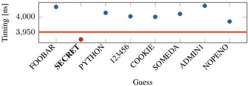Fig. 3: Decompression time with Decomp+Time for a dictionary attack. There is a clear threshold (line) separating the correct from wrong secrets. <details> <summary>Image 3 Details</summary>  ### Visual Description \n ## Scatter Plot: Timing vs. Guess ### Overview The image presents a scatter plot illustrating the relationship between a "Guess" (categorical variable) and "Timing" measured in nanoseconds (numerical variable). The plot displays timing measurements for several guesses, along with a horizontal line representing a threshold. ### Components/Axes * **X-axis:** Labeled "Guess". Categories are: FOOBAR, SECRET, PYTHON, 123456, COOKIE, SOMEDA, ADMINI, and NOPENO. * **Y-axis:** Labeled "Timing [ns]". The scale ranges from approximately 3400 ns to 4500 ns, with markings at 3500, 3600, 3700, 3800, 3900, 4000, 4100, 4200, 4300, 4400, and 4500. * **Data Points:** Blue circles representing timing measurements for each guess. * **Threshold Line:** A horizontal red line, positioned at approximately 3950 ns. ### Detailed Analysis The plot shows timing values for each guess. Let's analyze each data point: * **FOOBAR:** Timing is approximately 4250 ns. * **SECRET:** Timing is approximately 4200 ns. * **PYTHON:** Timing is approximately 3450 ns. This is a significant outlier, being the lowest timing value. * **123456:** Timing is approximately 4150 ns. * **COOKIE:** Timing is approximately 4000 ns. * **SOMEDA:** Timing is approximately 4100 ns. * **ADMINI:** Timing is approximately 4200 ns. * **NOPENO:** Timing is approximately 3800 ns. The red threshold line is at approximately 3950 ns. The guesses FOOBAR, SECRET, 123456, COOKIE, SOMEDA, and ADMINI all have timing values above this threshold. PYTHON and NOPENO have timing values below the threshold. ### Key Observations * The timing values are clustered between approximately 3450 ns and 4250 ns. * PYTHON has a significantly lower timing value than all other guesses, making it a clear outlier. * NOPENO has a timing value slightly below the threshold. * The other guesses (FOOBAR, SECRET, 123456, COOKIE, SOMEDA, ADMINI) all have timing values above the threshold. ### Interpretation This data likely represents a timing attack or a similar security analysis. The "Guess" values could be attempts to guess a password or key. The "Timing" represents the time taken to perform a comparison or operation. The threshold line (approximately 3950 ns) likely represents a baseline timing value. Guesses with timing values significantly *above* the threshold may indicate a correct guess, as the system might take longer to process a correct match. The outlier, PYTHON, having a much lower timing value, suggests it is likely an incorrect guess, or that the system handles it differently. The fact that most guesses are above the threshold suggests that the system is vulnerable to timing attacks, as an attacker could potentially determine the correct guess by observing the timing differences. The significant difference in timing for PYTHON could be due to optimizations or different code paths within the system. Further investigation would be needed to understand why PYTHON is so much faster. 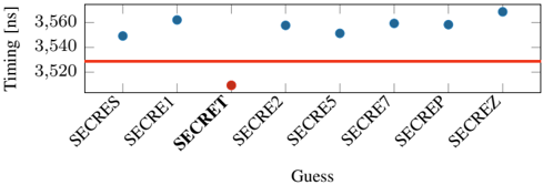</details> Fig. 4: Leaking the secret sixth offset character-wise. Still, the correct guess is distinguishable from the wrong guesses. A clear threshold can be used to separate the correct guess from the incorrect guesses. <details> <summary>Image 4 Details</summary>  ### Visual Description \n ## Scatter Plot: Timing vs. Guess ### Overview The image presents a scatter plot illustrating the relationship between "Guess" (labeled on the x-axis) and "Timing" measured in nanoseconds (ns), on the y-axis. The plot shows timing measurements for several guesses labeled "SECRET", "SECRET1" through "SECRET8". A horizontal line is also present, likely representing a threshold or baseline timing value. ### Components/Axes * **X-axis:** "Guess" with markers: SECRET, SECRET1, SECRET2, SECRET5, SECRET7, SECREPe, SECREZ. * **Y-axis:** "Timing [ns]" ranging from approximately 3520 ns to 3570 ns. * **Data Points:** Blue circles representing timing measurements for each guess. * **Threshold Line:** A horizontal red line. * **Outlier:** A single red data point for "SECRET2". ### Detailed Analysis The plot displays timing values for eight different guesses. The majority of the guesses ("SECRET", "SECRET1", "SECRET5", "SECRET7", "SECREPe", "SECREZ") exhibit timing values clustered between approximately 3550 ns and 3570 ns. The red horizontal line is positioned at approximately 3525 ns. Here's a breakdown of the approximate timing values for each guess: * SECRET: ~3555 ns * SECRET1: ~3552 ns * SECRET2: ~3522 ns (Red data point) * SECRET5: ~3558 ns * SECRET7: ~3562 ns * SECREPe: ~3560 ns * SECREZ: ~3568 ns The data points for "SECRET", "SECRET1", "SECRET5", "SECRET7", "SECREPe", and "SECREZ" are visually consistent, showing a relatively flat distribution. The timing for "SECRET2" is significantly lower than the others, falling below the red threshold line. ### Key Observations * "SECRET2" is a clear outlier, exhibiting a substantially lower timing value compared to all other guesses. * The timing values for the other guesses are relatively consistent, suggesting a similar processing time for those inputs. * The red horizontal line may represent a timing threshold, and "SECRET2" falls below this threshold. ### Interpretation The data suggests that the guess "SECRET2" is processed significantly faster than the other guesses. This could indicate a difference in the complexity of "SECRET2" compared to the others, or potentially a vulnerability or optimization related to that specific guess. The consistent timing values for the other guesses suggest a standard processing time for those inputs. The red line likely represents a performance benchmark or a security threshold. The fact that "SECRET2" falls below this threshold is noteworthy and warrants further investigation. It could be a sign of a successful attack or a unique characteristic of that particular guess. The plot demonstrates a potential timing-based side-channel vulnerability, where the time taken to process a guess reveals information about the guess itself. </details> Evaluation. Our evaluation was performed on an Intel i76700K (Ubuntu 20.04, kernel 5.4.0) with a fixed frequency of 4 GHz . To get stable results, we repeat the decompression step with each guess 10 000 times and repeat the entire attack 100 times. For each guess, we take the minimum timing difference per guess and choose the global minimum timing difference to determine the correct guess. Figure 3 illustrates the minimum decompression times. With zlib, we observe that the correct guess is faster on average by 71 . 5 ns ( n 100 , σ 27 . 91% ) compared to the second-fastest guess. Our attack correctly guessed the secret in all 100 repetitions of the attack. While we used a 6 B secret, our experiment also works for smaller secrets down to a length of 4 B . We also observe the attack is faster if the secret has a known prefix with a length of 3 B or more. Bytewise leakage. If the attacker manages to guess or know the first three bytes of the secret, the subsequent bytes can even be leaked bytewise using our attack. Both CRIME and BREACH, assume a known prefix such as cookie= . Similar to CRIME and BREACH [49], [20], [32], we try to perform a bytewise attack by modifying our simple layout. We use the first 5 characters of SECRET as a prefix "SECRE" and guess the last byte with 7 different guesses. On average the latency is 28 . 37 ns ( n 100 , σ 65 . 78% ), between the secret and second fastest guess. Figure 4 illustrates the minimum decompression times for the different guesses. However, we observe an error rate of 8 % for this experiment, which might be caused by the Huffmann-decoding part in DEFLATE. While techniques like the Two-Tries method [49], [20], [32] have been proposed to overcome the effects of Huffmancoding in DEFLATE to improve the fidelity of byte-wise attacks exploiting compression ratio, we seek to explore whether bytewise leakage can be reliably performed via the timing only by amplying the timing differences. 3) Challenge Of Amplifying Timing: While the decompression timing side channels can be directly used in attacks as demonstrated, the timing differences are still quite small for practical exploits on real-world applications. For example, the timing differences we observed for the correct guess are in tens of nanoseconds, while most practical use-cases of compression such as in a Memcached server accessed over the network, or PostgreSQL database accessed from a filesystem could have access latencies of milliseconds. Amplification. To enable memory compression attacks via the network or on data stored in file systems, we need to amplify the timing difference between correct and incorrect guesses. However, it is impractical to manually identify inputs that could amplify the timing differences, as each compression algorithm has a different implementation that is often highly optimized. Moreover, various input parameters could influence the timing of decompression, such as frequency of sequences, alignments of the secret and attack-controlled data, size of the input, entropy of the input, and different compression levels provided by algorithms. As an additional factor, the underlying hardware microarchitecture might also have undesirable influences. Therefore, to automate this process in a systematic manner, we develop an evolutionary fuzzer, Comprezzor, to find input corner cases that amplify the timing difference between correct and incorrect guesses for different compression algorithms. ## V. EVOLUTIONARY COMPRESSION-TIME FUZZER Compression algorithms are highly optimized, complex and even though most of them are open-source, their internals are only partially documented. Hence, we introduce Comprezzor, an evolutionary fuzzer to discover attacker-controlled inputs for compression algorithms that maximize differences in decompression times for certain guesses enabling both bytewise leakage and dictionary attacks. Comprezzor empowers genetic algorithms to amplify decompression side channels. It treats the decompression process of a compression algorithm as an opaque box and mutates inputs to the compression while trying to maximize the output, i.e. , timing differences for decompression with different guesses. The mutation process in Comprezzor focuses on not only the entropy of the data, but also the memory layout and alignment that end up triggering optimizations and slow paths in the implementation that are not easily detectable manually. While previous approaches used fuzzing to detect timing side channels [42], [27], Comprezzor can dramatically amplify timing differences by being specialized for compression algorithms by varying parameters like the input size, layout, and entropy that affect the decompression time. The inputs discovered by Comprezzor can amplify timing differences to such an extent that they are even observable remotely. ## A. Design of Comprezzor In this section, we describe the key components of our fuzzer: Input Generation, Fitness Function, Input Mutation and Input Evolution. Input Generation. Comprezzor generates memory layouts for Decomp+Time by maximizing the timing differences on decompression of the correct guess compared to incorrect ones. Comprezzor creates layouts with sizes in the range of 1 kB to 64 kB . It uses a helper program that takes the memory layout configuration as input, builds the requested memory layout for each guess, compresses them using the target compression algorithm, and reports the observed timing differences in the decompression times among the guesses. A memory layout configuration is composed of a file to start from, the offset of the secret in the file, the offset of guesses, how often the guesses are repeated in the layout, the compression level ( i.e. , between 1 and 9 for zlib), and a modulus for entropy reduction that reduces the range of the random values. The fuzzer can be used in cases where a prefix is known and unknown. Fitness Function. The evolutionary algorithm of Comprezzor starts from a random population of candidate layouts (samples) and takes as feedback the difference in time between decompression of the generated memory containing the correct guess and the incorrect ones. Comprezzor uses the timing difference between the correct guess and the second-fastest guess as the fitness score for a candidate. The fitness function is evaluated using a helper program performing an attack on the same setup as in Section IV-A. The program performs 100 iterations per guess and reports the minimum decompression time per guess to reduce the impact of noise. This minimum decompression time is the output of the fitness function for Comprezzor. Input Mutation. Comprezzor is able to amplify timing differences thanks to its set of mutations over the samples space specifically designed for data compression algorithms. Data compression algorithms leverage input patterns and entropy to shrink the input into a compressed form. For performance reasons, their ability to search for patterns in the input is limited by different internal parameters, like lookback windows, lookahead buffers, and history table sizes [46], [8]. We designed the mutations that affect the sample generation process to focus on input characteristics that directly impact compression algorithm strategies and limitations towards corner cases. Comprezzor mutations randomize the entropy and size of the samples that are generated. This has an effect on the overall compressibility of sequences and literals in the sample [8]. Moreover, the mutator varies the number of repeated guesses and their position in the resulting sample stressing the capability of the compression algorithm to find redundant sequences over different parts of the input. This affects the sequence compression and can lead to corner cases, i.e. , where subsequent blocks to be compressed are directly marked as incompressible, as we will later show for zlib in Section V-B. All of these factors together contribute to Comprezzor's ability to amplify timing differences. Input Evolution. Comprezzor follows an evolutionary approach to generate better inputs that maximize timing differences. It generates and mutates candidate layout configurations for the attack. Each configuration is forwarded to the helper program that builds the requested layout, inserts the candidate guess, compresses the memory, and returns the decompression time. Algorithm 1 shows the pseudocode of the evolutionary algorithm used by Comprezzor. ``` ``` Algorithm 1: Comprezzor evolutionary pseudo-code TABLE II: Timing differences between correct and incorrect guesses found by Comprezzor and the corresponding runtime. | Algorithm | Max difference for correct guess (ns) | Runtime (h) | |-------------|-----------------------------------------|---------------| | PGLZ | 109233 | 2.09 | | zlib | 71514.8 | 2.46 | | zstd | 4239.25 | 1.73 | | LZ4 | 2530.5 | 1.64 | Comprezzor iterates through different generations, with each sample having a probability of survival to the new generation that depends on its fitness score, where the fitness score is the time difference between the correct guess and the nearest incorrect one. Comprezzor discards all the samples where the correct guess is not the fastest or slowest. A retention factor decides the percentage of samples selected to survive among the best ones in the old generation ( 5 % by default). The population for each new generation is initialized with the samples that survived the selection process and enhanced by random mutations of such samples, tuning evolution towards local optimal solutions. By default, 70 % of the new population is generated by mutating the best samples from the previous generation. However, to avoid trapping the fuzzer in locally optimal solutions, a percentage of completely random new samples is injected in each new generation. Comprezzor runs until the maximum number of generations is evaluated, and the best candidate layouts found are returned. ## B. Results: Fuzzing Compression Algorithms Evaluation. Our test system has an Intel i7-6700K (Ubuntu 20.04, kernel 5.4.0) with a fixed frequency of 4 GHz . We run Comprezzor on four compression algorithms: zlib (1.2.11), Facebook's Zstd (1.5.0), LZ4 (v1.9.3), and PGLZ in PostgreSQL (v12.7). Comprezzor can support new algorithms by just adding compression and decompression functions. We run Comprezzor with 50 epochs and a population of 1000 samples per epoch. We set the retention factor to 5 % , selecting the best 50 samples in each generation of 1000 samples. We randomly mutate the selected samples to generate 70 % of the children and add 25 % of completely randomly generated layouts in the new generation. The runtime of Comprezzor to finish all 50 epochs was for zlib, 2 . 46 h , for zstd, 1 . 73 h , for LZ4, 1 . 64 h , and for PGLZ, 2 . 09 h . Table II lists the maximum timing differences found for Decomp+Time on the four compression algorithms, all of which use sequence compression like LZ77. Particularly, for zlib and PGLZ, the fuzzer discovers cases with timing differences of the scale of microseconds between correct and incorrect guesses, that is, orders of magnitude higher than the manually discovered differences in Section IV. Since zlib is one of the more popular algorithms, we analyze its high latency difference in more detail below. Zlib. Using Comprezzor, we found a corner case in zlib where all incorrect guesses lead to a slow code path, and the correct guess leads to a significantly faster execution time. We ran Comprezzor with a known prefix i.e. , cookie. We observe a high timing difference of 71 514 . 75 ns between correct and incorrect guesses, which is 3 orders of magnitude higher compared to the latency difference found manually in Section IV-C. This memory layout also leads to similarly high timing differences across all compression levels of zlib. To rule out micro-architectural effects, we re-run the experiment on different systems equipped with an Intel i5-8250U, AMD Ryzen Threadripper 1920X, and Intel Xeon Silver 4208, and observe similar timing differences. On further analysis, we observe that the corner case identified by the fuzzer is due to incompressible data. The initial data in the page, from a uniform distribution, is primarily incompressible. For such incompressible blocks, DEFLATE algorithm can store them as raw data blocks, also called stored blocks [12]. Such blocks have fast decompression times as only a single memcpy operation is needed on decompression instead of the actual DEFLATE process. In this particular corner case, the fuzzer discovered the correct guess results in such an incompressible stored block which is faster, while an incorrect guess results in a partly compressible input which is slower, as we describe below. Correct Guess. On a compression for the case where the guess matches the secret, the entire guess string, i.e. , cookie=SECRET , is compressed with the secret string. All subsequent data in the input is incompressible and treated as a stored block and decompressed with a single memcpy operation, which is fast without any Huffman or LZ77 decoding. Incorrect Guess. On a compression for the case where the guess does not match the secret, only the prefix of the guess, i.e. , cookie= , is compressed with the prefix of the secret, while another longer sequence i.e. , cookie=FOOBAR leads to forming a new block. On a decompression, this block must now undergo the Huffman decoding (and LZ77), which results in several table lookups, memory accesses, and higher latency. Thus, the timing differences for the correct and incorrect guesses are amplified by the layout that Comprezzor discovered. We provide more details about this layout in Figure 14 in the Appendix C and also provide listings of the debug trace from zlib for the decompression with the correct and incorrect guesses, to illustrate the root-cause of the amplified timing differences with this layout. Takeaway: We showed that it is possible to amplify timing differences for decompression timing attacks. With Comprezzor, we presented an approach to automatically find high timing differences in compression algorithms. The high latencies can be used for stable remote attacks. <details> <summary>Image 5 Details</summary>  ### Visual Description \n ## Diagram: Key-Value Store Data Flow ### Overview This diagram illustrates the data flow between a Sender, a Key-Value Store, and a Receiver. The Key-Value Store performs compression and decompression operations on the data. The diagram uses arrows to indicate the direction of data transfer and labels to describe the actions performed. ### Components/Axes The diagram consists of three main components: * **Sender:** Represented by a solid rectangle, positioned on the left side of the diagram. * **Key-Value Store:** Represented by a large light-blue rectangle in the center. It has a hatched section at the bottom. * **Receiver:** Represented by a rectangle filled with diagonal lines, positioned on the right side of the diagram. The following labels are present: * **Key-Value Store:** Located above the central rectangle. * **Compress/Decompress:** A curved label above the Key-Value Store, with a brace connecting it to the rectangle. * **Store/Update:** Labelled on the arrow originating from the Sender and pointing towards the Key-Value Store. * **Fetch data:** Labelled on the arrow originating from the Key-Value Store and pointing towards the Receiver. ### Detailed Analysis or Content Details The diagram shows a unidirectional data flow: 1. The Sender sends data to the Key-Value Store, labeled as "Store/Update". 2. The Key-Value Store processes the data, indicated by the "Compress/Decompress" label. The hatched section at the bottom of the Key-Value Store may represent stored data. 3. The Key-Value Store then sends data to the Receiver, labeled as "Fetch data". There are no numerical values or specific data points present in the diagram. It is a conceptual representation of a data flow process. ### Key Observations The diagram highlights the role of the Key-Value Store as an intermediary that handles data storage, updates, compression, and decompression. The use of arrows clearly indicates the direction of data transfer. The hatched section within the Key-Value Store suggests a storage component. ### Interpretation The diagram demonstrates a simplified model of how data is managed using a Key-Value Store. The Sender initiates a data operation (store or update), the Key-Value Store processes the data, and the Receiver retrieves the data. The compression/decompression step suggests that the Key-Value Store optimizes data storage and retrieval. This architecture is common in distributed systems and caching mechanisms where efficient data access is crucial. The diagram does not specify the type of data being stored or the specific compression algorithms used. It is a high-level overview of the data flow, focusing on the core components and their interactions. </details> Fig. 5: Covert communication via a key-value store using memory compression. <details> <summary>Image 6 Details</summary>  ### Visual Description \n ## Chart: Response Time Distribution by Entropy ### Overview The image presents a line chart illustrating the distribution of response times for two entropy levels: "Lower entropy" and "Higher entropy". The x-axis represents response time in nanoseconds (ns), and the y-axis represents the amount or frequency of occurrences. ### Components/Axes * **X-axis:** Response time [ns] (scaled from approximately 0.6 x 10⁴ to 1.2 x 10⁴). * **Y-axis:** Amount (scaled from 0 to 600). * **Legend:** Located in the top-center of the chart. * "Lower entropy (0x42-4096)" - represented by a dotted black line. * "Higher entropy" - represented by a solid red line. ### Detailed Analysis The chart displays two distinct peaks, one for each entropy level. **Lower Entropy (dotted black line):** The line shows a peak around 0.7 x 10⁴ ns. The amount at the peak is approximately 500. The distribution is concentrated within a narrow range, from approximately 0.66 x 10⁴ ns to 0.74 x 10⁴ ns. The line quickly descends to zero on either side of the peak. **Higher Entropy (solid red line):** The line shows a peak around 1.05 x 10⁴ ns. The amount at the peak is approximately 480. The distribution is also concentrated, but slightly broader than the lower entropy distribution, ranging from approximately 0.98 x 10⁴ ns to 1.12 x 10⁴ ns. The line quickly descends to zero on either side of the peak. ### Key Observations * The response times for lower entropy are significantly faster (around 0.7 x 10⁴ ns) than those for higher entropy (around 1.05 x 10⁴ ns). * Both distributions are relatively narrow, indicating a consistent response time within each entropy level. * The amount (frequency) of occurrences is comparable for both entropy levels, with the peak amounts being approximately 500 and 480 respectively. ### Interpretation The data suggests that lower entropy conditions lead to faster response times compared to higher entropy conditions. This could be due to several factors, such as reduced computational complexity or more predictable system behavior under lower entropy. The narrow distributions indicate that the system is relatively stable and consistent within each entropy level. The peaks represent the most common response times for each condition. The difference in peak locations (0.7 x 10⁴ ns vs 1.05 x 10⁴ ns) is a clear indicator of the impact of entropy on response time. The values "0x42-4096" in the legend for lower entropy likely represent a specific configuration or seed value used to generate the lower entropy condition. This chart is likely demonstrating the performance impact of entropy on a system, potentially related to randomness or unpredictability in the system's operation. </details> Fig. 6: Timing when decompressing a single zlib-compressed 4 kB page with a high-entropy in comparison to a page with a low-entropy. ## VI. CASE STUDIES In this section, we present three case studies showing the security impacts of the timing side channel. In Section VI-A, we present a local covert channel that allows hidden communication via the latency decompression. Furthermore, we present a remote covert channel that exploits the decompression of memory objects in a PHP application using Memcached. We demonstrate Decomp+Time on a PHP application that compresses secret data together with attacker-data to leak the secret bytewise. In Section VI-D, we leak inaccessible values from a database, exploiting the internal compression of PostgreSQL. In Section VI-E, we show that OS-based memory compression also has timing side channels that can leak secrets. ## A. Covert channel To evaluate the transmission capacity of memorycompression attacks, we evaluate the transmission rate for a covert channel, where the attacker controls both the sending and receiving end. First, we evaluate a cross-core covert channel that relies on shared memory. This is in line with state-of-theart work to measure the maximum capacity of the memory compression side channel [24], [35], [37], [62], [23], [25]. The maximum capacity poses a leakage rate limit for other attacks that use memory compression as a side channel. Our local covert channel achieves a capacity of 448 bit ♥ s ( n 100 , σ 0 . 001% ). 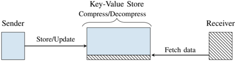Setup. Figure 5 illustrates the covert communication between a sender and receiver via shared memory. We create a simple key-value store that communicates via UNIX sockets. The store takes input from a client and stores it on a 4 kB -aligned page. The sender inserts a key and value into the first page to communicate with the server. The receiver inserts a small key and value as well, which should be placed on the same 4 kB . If the 4 kB -page is fully written, the key-value store compresses the whole page. Compressing full 4 kB -page separately also occurs on filesystems like BTRFS [6]. 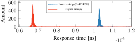Sender and receiver agree on a time frame to send and read content. The basic idea is to communicate via the observation on zlib that memory with low entropy, e.g., 4096 times the same value, requires more time when decompressing compared to pages with a higher entropy, e.g., repeating sequence number from 0 to 255 . Figure 6 shows the histogram of latency when decompression is triggered for both cases for the key-value on an Intel i7-6700K running at 4 GHz . On average, we observe a timing difference of 3566 . 22 ns ( 14 264 . 88 cycles, n 100000 ). These two timing differences are easy to distinguish and enable covert communication. Transmission. We evaluate our cross-core covert channel by generating and sending random content from /dev/urandom through the memory compression timing side channel. The sender transmits a '1'-bit by performing a store with the page that has a higher entropy 4095 B in the key-value store. Conversely, to transmit a '0'-bit, the sender compresses a lowentropy 4 kB page. To trigger the compression, the receiver also stores a key-value pair in the page, wheres as 1 B fills the remaining page. The key-value store will now compress the full 4 kB -page, as it is fully used. The receiver performs a fetch request from the key-value store, which triggers a decompression of the 4 kB -page. To distinguish bits, the receiver measures the mean RTT of the fetch request. Evaluation. Our test machine is equipped with an Intel Core i7-6700K (Ubuntu 20.04, kernel 5.4.0), and all cores are running on a fixed CPU frequency of 4 GHz . We repeat the transmission 50 times and send per run 640 B . To reduce the error rate, the receiver fetches the receiver-controlled data 50 times and compares the average response time against the threshold. Our cross-core covert channel achieves an average transmission rate of 448 bit ♥ s ( n 100 , σ 0 . 007% ) with an error rate of 0 . 082 % ( n 100 , σ 2 . 85% ). This capacity of the unoptimized covert channel is comparable to other stateof-the-art microarchitectural cross-core covert channels that do not rely on shared memory [60], [36], [14], [44], [37], [53], [47], [59]. ## B. Remote Covert Channel We extend the scope of our covert channel to a remote covert channel. In the remote scenario, we rely on Memcached on a web server for memory compression and decompression. Memcached. Memcached is a widely used caching system for web sites [38]. Memcached is a simple key-value store that internally uses a slab allocator. A slab is a fixed unit of contiguous physical memory, which is typically assigned to a certain slab class which is typically a 1 MB region [29]. Certain programming languages such as PHP or Python offer the option to compress memory before it is stored in Memcached [45], [5]. For PHP, memory compression is enabled per default if Memcached is used [45]. PHP-Memcached has a threshold that decides at which size data is compressed, with the default value at 2000 B . Furthermore, PHP-Memcached computes the compression ratio to a compression factor and decides whether it stores the data compressed or uncompressed in Memcached. The default value for the compression factor is 1 . 3 , i.e. , 23 % of the space needs to be saved from the original data size to store it compressed [45]. Fig. 7: Distribution of HTTP response times for zlibdecompressed pages stored in Memcached on memory compression encoding a '1' and a '0'-bit. <details> <summary>Image 7 Details</summary>  ### Visual Description \n ## Line Chart: Response Time vs. Amount ### Overview The image presents a line chart illustrating the relationship between Response Time (in nanoseconds) and Amount. Two distinct data series are plotted, likely representing different conditions or categories. The chart appears to show the distribution of "Amount" over a range of "Response Time" values. ### Components/Axes * **X-axis:** "Response time [ns] ⋅10⁶". Scale ranges from approximately 0.4 to 2.0, with tick marks at 0.6, 0.8, 1.0, 1.2, 1.4, 1.6, 1.8, and 2.0. * **Y-axis:** "Amount". Scale ranges from 0 to 400, with tick marks at 0, 100, 200, 300, and 400. * **Legend:** Located in the top-right corner. * "0" - Represented by a dotted blue line. * "1" - Represented by a solid red line. ### Detailed Analysis * **Data Series 0 (Blue Dotted Line):** This line starts at approximately 0 at a response time of 0.4 ns. It increases gradually, reaching a peak of approximately 320 at a response time of around 0.95 ns. After the peak, the line decreases rapidly, crossing the 0 amount level around 1.3 ns. It remains near 0 for the rest of the plotted range. * **Data Series 1 (Red Solid Line):** This line starts at approximately 0 at a response time of 0.4 ns. It increases sharply, reaching a peak of approximately 390 at a response time of around 0.9 ns. The line then decreases more gradually than Data Series 0, reaching approximately 230 at 1.1 ns, and then continues to decrease, approaching 0 around 1.6 ns. It remains near 0 for the rest of the plotted range. ### Key Observations * Both data series exhibit a similar trend: an initial increase followed by a decrease. * Data Series 1 (red line) has a higher peak amount and a slower decay compared to Data Series 0 (blue line). * The peak of Data Series 1 occurs slightly earlier in time than the peak of Data Series 0. * Both series converge to approximately 0 amount at higher response times. ### Interpretation The chart likely represents the distribution of some event or quantity ("Amount") as a function of the time it takes to respond ("Response Time"). The two data series could represent different conditions or treatments. The higher peak and slower decay of Data Series 1 suggest that, under condition "1", the event occurs more frequently and persists for a longer duration compared to condition "0". The initial faster rise of Data Series 1 could indicate a quicker initial response. The convergence of both series at higher response times suggests that, eventually, the event becomes negligible regardless of the condition. The chart could be illustrating the response of a system to a stimulus, the decay of a signal, or the distribution of reaction times in an experiment. Without further context, it's difficult to determine the precise meaning of the data, but the chart clearly demonstrates a difference in the temporal characteristics of the event under the two conditions. </details> Bypassing the Compression Factor. While the compression factor already introduces a timing side channel, we focus on scenarios where data is always compressed. This is later useful for leakage on co-located data. Intuitively, it should suffice to prepend highly-compressible data to enforce compression. However, we found that only prepending and adopting the offsets for secret repetitions, as for zlib, also influenced the corner case we found and the large timing difference. We integrate prepending of compressible pages to Comprezzor and also add the compression factor constraint to automatically discover inputs that fulfills the constraint and leads to large latencies between a correct and incorrect guess. Transmission. We use the page found by Comprezzor which triggers a significantly lower decompression time to encode a '1'-bit. Conversely, for a '0'-bit, we choose content that triggers a significantly higher decompression time. The sender places a key-value pair for each bit index at once into PHPMemcached. The receiver sends GET requests to the resource, causing decompression of the data that contains the sender content. The timing difference of the decompression is reflected in the RTT of the HTTP request. Hence, we measure the timing difference between the HTTP request being sent and the first response packet received. Evaluation. Our sender and receiver are equipped with an Intel i7-6700K (Ubuntu 20.04, kernel 5.4.0) and connected to the internet with a 10 Gb/s connection. For the web server, we use a dedicated server in the Equinix [13] cloud, 14 hops away from our network (over 1000 km physical distance) with a 10 Gbit ♥ s connection. The victim server is equipped with an Intel Xeon E3-1240 v5 (Ubuntu 20.04, kernel 5.4.0). Our server runs a PHP (version 7.4) website, which allows storing and retrieving data, backed by Memcached. We installed Memcached 1.5.22, the default version on Ubuntu 20.04. The PHP website is hosted on Nginx 1.18.0 with PHP-FPM. 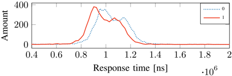We perform a simple test where we perform 5000 HTTP requests to a PHP site that stores zlib-compressed memory in Memcached. Figure 7 illustrates the timing difference between a '0'-bit and a '1'-bit. The timing difference between the mean values for a '0'- and '1'-bit is 61 622 . 042 ns . Figure 7 shows that the two distributions overlap to a certain extent. We call this overlap the critical section . We implement an early-stopping mechanism for bits in the covert channel that clearly belong into one of the two regions below or above the critical section. After 25 requests, we start to classify the RTT per bit. Fig. 8: Distribution of the response time for the correct guess (S) and the incorrect guesses (0-9, A-R, T-Z) for the first byte leaked in the byte-wise leakage of the secret from PHPMemcached. Similar trends are observed for subsequent bytes leaked as shown in Appendix D. <details> <summary>Image 8 Details</summary>  ### Visual Description \n ## Scatter Plot: Timing vs. Guess (Byte 0) ### Overview This image presents a scatter plot illustrating the relationship between a "Guess" value (representing potential cookie values) and "Timing" measured in nanoseconds (ns). The plot focuses on Byte 0 of a larger dataset, as indicated by the title "Byte 0". The data points appear to represent timing measurements associated with different guess values. ### Components/Axes * **X-axis:** "Guess" - Categorical variable with the following values: "cookie=0", "cookie=5", "cookie=9", "cookie=A", "cookie=H", "cookie=M", "cookie=S", "cookie=Z". * **Y-axis:** "Timing [ns]" - Numerical variable, ranging from approximately 1.00 x 10⁶ ns to 1.07 x 10⁶ ns. * **Title:** "Byte 0" - Indicates the data pertains to the first byte. * **Data Points:** Blue circles representing timing measurements for each guess value. * **Outlier:** A single red circle at "cookie=S" with a timing of approximately 1.00 x 10⁶ ns. ### Detailed Analysis The scatter plot shows a relatively consistent timing value across most guess values. The majority of the blue data points cluster between approximately 1.02 x 10⁶ ns and 1.06 x 10⁶ ns. Here's a breakdown of approximate timing values for each guess: * **cookie=0:** Timing values range from approximately 1.02 x 10⁶ ns to 1.05 x 10⁶ ns. * **cookie=5:** Timing values range from approximately 1.03 x 10⁶ ns to 1.06 x 10⁶ ns. * **cookie=9:** Timing values range from approximately 1.03 x 10⁶ ns to 1.06 x 10⁶ ns. * **cookie=A:** Timing values range from approximately 1.03 x 10⁶ ns to 1.06 x 10⁶ ns. * **cookie=H:** Timing values range from approximately 1.03 x 10⁶ ns to 1.06 x 10⁶ ns. * **cookie=M:** Timing values range from approximately 1.03 x 10⁶ ns to 1.06 x 10⁶ ns. * **cookie=S:** Timing value is approximately 1.00 x 10⁶ ns (red outlier). * **cookie=Z:** Timing values range from approximately 1.03 x 10⁶ ns to 1.05 x 10⁶ ns. ### Key Observations * The timing values are relatively stable across most guess values. * The "cookie=S" guess exhibits a significantly lower timing value compared to all other guesses, and is highlighted in red. This is a clear outlier. * There is no obvious linear trend or correlation between the guess value and the timing. ### Interpretation The data suggests that the timing measurements are largely unaffected by the guessed cookie value, *except* for "cookie=S". The significantly lower timing for "cookie=S" indicates that this guess is likely the correct value, or at least a value that triggers a faster processing path. This could be due to a timing attack vulnerability where the system responds faster when the correct guess is made. The consistent timing for other guesses suggests that the system is designed to obfuscate the correct guess by introducing a constant delay. The outlier at "cookie=S" is a strong indicator of a potential security weakness. The plot demonstrates a timing difference that could be exploited to determine the correct cookie value. The fact that the data is presented for "Byte 0" suggests that this is part of a larger analysis of the entire cookie. </details> At most, we perform 200 HTTP requests per bit. If there are still unclassified bits, we compare the amount of requests classified as '0'-bit and those classified as '1'-bit and decide on the side with more elements. We transmit a series of different messages of 8 B over the internet. Our simple remote covert channel achieves an average transmission rate of 643 . 25 bit ♥ h ( n 20 , σ 6 . 66% ) at an average error rate of 0 . 93 % . Our covert channel outperforms the one by Schwarz et al. [52] and Gruss [22],although our attack works with HTTP instead of the more lightweight UDP sockets. Other remote timing attacks usually do not evaluate their capacity with a remote covert channel [65], [30], [2], [51], [1], [2], [56]. ## C. Remote Attack on PHP-Memcached Using our building blocks to perform Decomp+Time and the remote covert channel, we perform a remote attack on PHP-Memcached to leak secret data from a server over the internet. We assume a memory layout where secret memory is co-located to attacker-controlled memory, and the overall memory region is compressed. 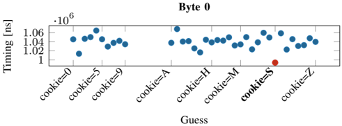Attack Setup. We use the same PHP-API as in Section VI-B that allows storing and retrieving data. We run the attack using the same server setup as used for the remote covert channel attacking a dedicated server in the Equinix [13] cloud 14 hops away from our network. We define a 6 B long secret ( SECRET ) with a 7 B long prefix ( cookie= ) and prepend it to the stored data of users. PHP-Memcached will compress the data before storing it in Memcached and decompress it when accessing it again. For each guess, the PHP application stores the uploaded data to a certain location in Memcached. On each data fetch, the PHP application decompresses the secret data together with the co-located attacker-controlled data and then responds onlythe attacker-controlled data. The attacker measures the RTT per guess and distinguishes the timing differences between the guesses. In the case of zlib, the guess with the fastest response time is the correct guess. We demonstrate a byte-wise leakage of an arbitrary secret and also a dictionary attack with a dictionary size of 100 guesses. Evaluation. For the byte-wise attack, we assume each byte of the secret is from 'A-Z,0-9' (36 different options). For each of the 6 bytes to be leaked, we generate a separate memory layout using Comprezzor that maximizes the latency between the guesses. We repeat the experiment 20 times. On average, our attack leaks the entire 6 B secret string in 31 . 95 min ( n Fig. 9: Distribution of the response time for the correct guess (SECRET) and the 99 other incorrect guesses in dictionary attack on PHP-Memcached. Note that we only label SECRET and 6 out of 99 incorrect guesses on the X-axis for brevity. 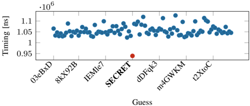<details> <summary>Image 9 Details</summary>  ### Visual Description \n ## Scatter Plot: Timing vs. Guess ### Overview This image presents a scatter plot visualizing the relationship between "Guess" values on the x-axis and "Timing" in nanoseconds (ns) on the y-axis. The plot displays a series of data points, with one outlier significantly deviating from the general trend. ### Components/Axes * **X-axis Label:** "Guess" * Categories: 03eBxD, 8kX92B, IEMle7, SECRET, dDFqk3, m4GWKM, l2XtoC * **Y-axis Label:** "Timing [ns]" (Timing in nanoseconds) * Scale: Ranges approximately from 0.95 x 10⁶ ns to 1.12 x 10⁶ ns. * **Data Points:** Blue circles representing timing measurements for each guess. * **Outlier:** A single red circle, visually distinct from the blue data points. ### Detailed Analysis The majority of the data points cluster between approximately 1.03 x 10⁶ ns and 1.1 x 10⁶ ns. The data points appear relatively scattered with no strong linear trend. Let's analyze the data points for each "Guess" category: * **03eBxD:** Timing values range from approximately 1.04 x 10⁶ ns to 1.08 x 10⁶ ns. * **8kX92B:** Timing values range from approximately 1.03 x 10⁶ ns to 1.09 x 10⁶ ns. * **IEMle7:** Timing values range from approximately 1.04 x 10⁶ ns to 1.1 x 10⁶ ns. * **SECRET:** Timing value is approximately 0.96 x 10⁶ ns (the outlier, marked in red). * **dDFqk3:** Timing values range from approximately 1.04 x 10⁶ ns to 1.1 x 10⁶ ns. * **m4GWKM:** Timing values range from approximately 1.03 x 10⁶ ns to 1.08 x 10⁶ ns. * **l2XtoC:** Timing values range from approximately 1.04 x 10⁶ ns to 1.08 x 10⁶ ns. The outlier, "SECRET", has a timing value significantly lower than all other guesses, at approximately 0.96 x 10⁶ ns. ### Key Observations * The timing values for most guesses are relatively consistent, fluctuating within a narrow range. * The "SECRET" guess exhibits a dramatically lower timing value, making it a clear outlier. * There is no obvious correlation between the "Guess" category and the "Timing" value, except for the outlier. ### Interpretation The data suggests that the timing performance is generally stable across different "Guess" values. However, the "SECRET" guess stands out as an anomaly, indicating significantly faster processing or execution time compared to the others. This could be due to several factors: * **Optimization:** The "SECRET" guess might be optimized for faster processing. * **Algorithm:** The algorithm used for the "SECRET" guess might be more efficient. * **Data Characteristics:** The data associated with the "SECRET" guess might have properties that lead to faster processing. * **Error:** There is a possibility of an error in the measurement or recording of the timing value for "SECRET". Further investigation is needed to understand the underlying reasons for this significant difference in timing performance. The outlier suggests a potential area for optimization or a unique characteristic of the "SECRET" guess that warrants further analysis. </details> 20 , σ 8 . 48% ). Since the latencies between a correct and incorrect guess are in the microseconds range, we do not observe false positives with our approach. Figure 8 shows the median response time for each guess in the first iteration (leaking the first byte) as a representative example. It can be seen that the response time for the correct guess ( S ) for the first byte is significantly faster than the incorrect guesses. We observe similar results for the remaining bytes ( E,C,R,E,T ). Dictionary attack. While bytewise leakage is the more generic and practical approach for decompression timing attacks, there might be use cases where also a dictionary attack is applicable. For instance, if the attacker would try the top n most common usernames or passwords, which are publicly available. Another use case for dictionary attacks could be to profile if certain images are forbidden in a database used for digital rights management. We perform a dictionary attack over the network using randomly generated 100 guesses, including the correct guess. We repeat the experiment 20 times. For each run, we re-generate the guesses and randomly shuffle the order of the guesses per request iteration to not create a potential bias. On average, our attack leaks the secret string in 14 . 99 min ( n 20 , σ 16 . 27% ). To classify the correct guess, we use the same early stopping technique as was used for the covert channel. Since the timing difference is in the microseconds range, we do not observe false positives with our approach. Figure 9 illustrates the median of the response times for each guess from one iteration. Figure 15 (in Appendix D) shows the latencies for all leaked bytes. It can be clearly seen that the response time for the correct guess ( SECRET ) is significantly faster. Takeaway: We show that a PHP application using Memcached to cache blobs hosted on Nginx enables covert communication with a transmission rate of 643 . 25 bit ♥ h . If secret data is stored together with attacker-controlled data, we demonstrate a remote memory-compression attack on Memcached leaking a 6 B -secret bytewise in 31 . 95 min . We further demonstrated that the attack can also be used for dictionary attacks. ## D. Leaking Data from Compressed Database In this section, we show that an attacker can also exploit compression in databases to leak inaccessible information, i.e. , from the internal database compression of PostgreSQL. PostgreSQL Data Compression. PostgreSQL is a widespread open-source relational database system using the SQL standard. PostgreSQL maintains tuples saved on disk using a fixed page size of commonly 8 kB , storing larger fields compressed and possibly split into multiple pages. By default, variable-length fields that may produce large values, e.g., TEXT fields, are stored compressed. PostgreSQL's transparent compression is known as TOAST (The OversizedAttribute Storage Technique) and uses a fast LZ-family compression, PGLZ [46]. By default, data in a cell is actually stored compressed if such a form saves at least 25 % of the uncompressed size to avoid wasting decompression time if it is not worth it. Indeed, data stored uncompressed is accessed faster than data stored compressed since the decompression algorithm is not executed. Moreover, the decompression time depends on the compressibility of the underlying data. A potential attack scenario for structured text in a cell is where JSON documents are stored and compressed within a single cell, and the attacker controls a specific field within the document. While our focus is restricted to cell-level compression, note that compressed columnar storage [9], [39], [7], a non-default extension available in PostgreSQL, may also be vulnerable to decompression timing attacks. Attack Setup. To assess the feasibility of an attack, we use a local database server and access two differently compressed rows with a Python wrapper using the psycopg2 library. The first row contains 8192 characters of highly compressible data, while the second one 8192 characters of random incompressible data. Both rows are stored in a table as TEXT data and accessed 1000 times. The median for the number of clock cycles required to access the compressible row is 249 031 , while for the uncompressed one is 221 000 , which makes the two accesses distinguishable. On our 4 GHz CPUs, this is a timing difference of 7007 . 75 ns . We use Comprezzor to amplify these timing differences and demonstrate a bytewise leakage of a secret and also a dictionary attack. Leaking First Byte. For the bytewise leeakage of the secret, we first create a memory layout to leak the first byte using Comprezzor against a standalone version of PostgreSQL's compression library, using a similar setup as the previous Memcached attack. A key difference in the use of Comprezzor with PostgreSQL is that the helper program measuring the decompression time returns a time of 0 when the input is not compressed, i.e. , the data compressed with PGLZ does not save at least 25 % of the original size. Comprezzor found a layout that sits exactly at the corner case where a correct guess in the secret results in a compressed size that saves 25 % of the original size. Hence, a correct guess is saved compressed, while for any wrong guess, the threshold is not met, and the data is saved uncompressed. This is because the correct guess characters match the secret bytes and result in a higher compression rate. Leaking Subsequent Bytes with Secret Shifting. We observed that one good layout is enough and can be reused for bytewise leakage in PGLZ. The prefix can be shifted by one character to the left by a single character, i.e. , from 'cookie=S' to 'ookie=SE', to accommodate an additional byte for the guess. This shifting allows bytewise leakage with the same memory layout. Note, that the same approach did not work Fig. 10: Distribution of the response time for the first-byte guesses in the remote PostgreSQL attack leaking a secret bytewise, with the correct guess (S) and incorrect guesses (0-9, A-R, T-Z). Similar trends are observed for subsequent bytes leaked as shown in Appendix D. 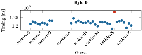<details> <summary>Image 10 Details</summary>  ### Visual Description \n ## Scatter Plot: Timing vs. Guess (Byte 0) ### Overview This image presents a scatter plot illustrating the relationship between "Guess" values (representing potential cookie values) and "Timing" measurements in nanoseconds (ns). The plot focuses on Byte 0 of a cookie. The majority of data points cluster around a relatively consistent timing value, with a single outlier significantly deviating from this pattern. ### Components/Axes * **X-axis:** "Guess" - Categorical variable representing potential cookie values. The categories are: "cookie=0", "cookie=5", "cookie=9", "cookie=A", "cookie=H", "cookie=M", "cookie=S", "cookie=Z". * **Y-axis:** "Timing [ns]" - Numerical variable representing the time taken, measured in nanoseconds. The scale ranges from approximately 1.18 x 10⁶ ns to 1.26 x 10⁶ ns. * **Data Points:** Blue circles represent the timing measurements for each guess. * **Outlier:** A single red circle represents a significantly higher timing measurement. * **Title:** "Byte 0" - Indicates the plot represents data for the first byte of a cookie. ### Detailed Analysis The majority of the data points (blue circles) exhibit a relatively stable timing value, fluctuating between approximately 1.20 x 10⁶ ns and 1.24 x 10⁶ ns. There is a slight undulating pattern, with minor peaks and troughs across the different "Guess" values. Here's a breakdown of approximate timing values for each guess: * **cookie=0:** ~1.22 x 10⁶ ns * **cookie=5:** ~1.23 x 10⁶ ns * **cookie=9:** ~1.21 x 10⁶ ns * **cookie=A:** ~1.24 x 10⁶ ns * **cookie=H:** ~1.24 x 10⁶ ns * **cookie=M:** ~1.22 x 10⁶ ns * **cookie=S:** ~1.19 x 10⁶ ns * **cookie=Z:** ~1.21 x 10⁶ ns The outlier (red circle) is located at "cookie=S" and has a timing value of approximately 1.255 x 10⁶ ns. This is significantly higher than all other data points. ### Key Observations * The timing values are relatively consistent across most "Guess" values. * The outlier at "cookie=S" represents a substantial deviation from the typical timing behavior. * There is no clear monotonic trend (increasing or decreasing) in the timing values as the "Guess" values change. ### Interpretation This data likely represents a timing attack scenario, where the attacker attempts to guess the value of a cookie byte by measuring the time it takes for a server to respond. The consistent timing values for most guesses suggest that the server is not significantly affected by the input value. However, the outlier at "cookie=S" indicates that this particular guess triggers a different code path or operation that takes considerably longer to execute. This could be due to a conditional statement, a cache miss, or other performance-sensitive factors. The attacker could use this information to narrow down the possible values of the cookie byte. The outlier provides a strong indication that "cookie=S" is a likely candidate. This type of analysis is crucial in identifying and mitigating timing vulnerabilities in security-sensitive applications. The fact that only Byte 0 is shown suggests this is part of a larger analysis of all cookie bytes. </details> Fig. 11: Distribution of the response time in the remote PostgreSQL dictionary attack, for the correct guess (SECRET) and the 99 other incorrect guesses (we only label 4 out of 99 incorrect guesses and SECRET on the X-axis for brevity). 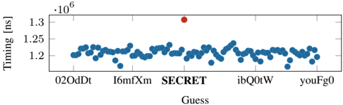<details> <summary>Image 11 Details</summary>  ### Visual Description \n ## Scatter Plot: Timing vs. Guess ### Overview This image presents a scatter plot visualizing the relationship between "Guess" values on the x-axis and "Timing" in nanoseconds (ns) on the y-axis. The plot displays a series of data points, with one outlier significantly deviating from the general trend. ### Components/Axes * **X-axis:** Labeled "Guess". The categories displayed are: "02OdDt", "l6mfXm", "SECRET", "ibQ0tW", and "youFg0". * **Y-axis:** Labeled "Timing [ns]". The scale ranges from approximately 1.20 x 10⁶ ns to 1.30 x 10⁶ ns. * **Data Points:** Represented by blue circles. * **Outlier:** A single red circle, visually distinct from the blue data points. ### Detailed Analysis The majority of the data points cluster between approximately 1.21 x 10⁶ ns and 1.27 x 10⁶ ns. The data appears somewhat scattered, with no strong linear trend visible across the majority of the points. Let's analyze the data points for each "Guess" category: * **02OdDt:** Timing values range from approximately 1.21 x 10⁶ ns to 1.26 x 10⁶ ns. * **l6mfXm:** Timing values range from approximately 1.19 x 10⁶ ns to 1.25 x 10⁶ ns. * **SECRET:** This category contains the outlier. The timing value is approximately 1.31 x 10⁶ ns. * **ibQ0tW:** Timing values range from approximately 1.22 x 10⁶ ns to 1.27 x 10⁶ ns. * **youFg0:** Timing values range from approximately 1.21 x 10⁶ ns to 1.26 x 10⁶ ns. The outlier, associated with the "SECRET" guess, is significantly higher in timing than all other data points. ### Key Observations * The "SECRET" guess exhibits a substantially longer timing compared to all other guesses. This is a clear outlier. * The timing values for the other guesses ("02OdDt", "l6mfXm", "ibQ0tW", "youFg0") are relatively consistent, with some variation within each category. * There is no obvious correlation between the "Guess" category and the timing value, except for the outlier. ### Interpretation The data suggests that the process being measured (timing) is generally consistent across different "Guess" values. However, the "SECRET" guess triggers a significantly longer timing, indicating a potential difference in the underlying process or a specific characteristic associated with that guess. This could be due to a more complex computation, a different code path, or some other factor that increases the execution time. The outlier is a critical observation. It suggests that the "SECRET" guess is somehow special or requires a different handling mechanism, leading to the increased timing. Further investigation is needed to understand why this occurs. The data could be related to a side-channel attack or a security vulnerability where the timing reveals information about the secret. The fact that the timing is so much higher for "SECRET" is a strong indicator of something unusual happening during the processing of that guess. </details> on DEFLATE. We leave it as future work, to mount such a shifting approach to other compression algorithms. Evaluation. We perform a remote decompression timing attack against a Flask [17] web server that uses a PostgreSQL database to store user-provided data. We used the same Equinix cloudserver setup as used for the Memcached remote attack (cf. Section VI-C). The server runs Python 3.8.5 with Flask version 2.0.1 and PostgreSQL version 12.7. We define a 6 B long-secret with a 7 B prefix that the server colocates with attacker-provided data in a cell of the database through POST requests. The secret is never shown to the user. Using the layout found by Comprezzor, the entry in the database is stored compressed only when the secret matches in the provided data. A second endpoint in the server accesses the database to read the data without returning the secret to the attacker. The attack leaks bytewise over the internet by guessing again in the character set 'A-Z,0-9' ( 36 possibilities per character), including the correct one. We repeat the attack 20 times. The average time required to determine the guess with the highest latency (that the server had to decompress before returning) is 17 . 84 min ( 2 . 97 min ♥ B ) ( n 20 , σ 2 . 3% ). Figure 10 illustrates the median of the response times for a single guess in an example iteration, showing how the correct guess results in a slower response. Dictionary attack. We also performed a dictionary attack over the internet with 100 randomly generated guesses, including the correct one, and repeated the experiments 20 times. We measured the time required for the server to reply to a request in the second endpoint by observing the network packets arriving at our machine with the same setup as the remote Memcached attack, repeating each request 100 times. The average time required to brute-force all the guesses and select the guess with the highest latency (that the server had to decompress before returning) is 8 . 28 min ( n 20 , σ 0 . 003% ). Figure 11 illustrates the median of the response times for each guess in an example iteration, showing how the correct guess results in a slower response. Again, the timing difference is clearly distinguishable over 14 h ops in the internet. Takeaway: Secrets can be leaked from databases due to timing differences caused by PostgreSQL's transparent compression, if an application stores untrusted data with secrets in the same cell of a database. With a Flask appplication using a PostgreSQL database, we show that an attacker can infer when its inserted data matches the secret based on response times, which are influence by the decompression timing. Our decompression timing attack on PostgreSQL leaks a 6 B secret bytewise over the network in 17 . 84 min . ## E. Attacking OS Memory Compression In this section, we show how memory compression in modern OSs can introduce exploitable timing differences. In particular, we demonstrate a dictionary-based attack to leak secrets from compressed pages in ZRAM, the Linux implementation of memory compression. Background. Memory compression is a technique used in many modern OSs, e.g., Linux [34], Windows [28], or MacOS [11]. Similar to traditional swapping, memory compression increases the effective memory capacity of a system. When processes require more memory than available, the OS can transparently compress unused pages in DRAM to ensure they occupy a smaller footprint in DRAM rather than swapping them to disk. This frees up memory while still allowing the compressed pages to be accessed from DRAM. Compared to disk I/O, DRAM access is an order of magnitude faster, and even with the additional decompression overhead, memory compression is significantly faster than swapping. Hence, memory compression can improve the performance despite the additional CPU cycles required for compression and decompression. Such memory compression is adopted in the Linux kernel (since kernel version 3.14) in a module called ZRAM [26], which is enabled by default on Fedora [34] and Chrome OS [11]. 1) Characterizing Timing Differences in ZRAM: To understand how memory compression can be exploited, we characterize its behavior in ZRAM. On Linux systems, ZRAM appears as a DRAM-backed block device. When pages need to be swapped to free up memory, they are instead compressed and moved to ZRAM. Subsequent accesses to data in ZRAM result in a page fault, and the page is decompressed from ZRAM and copied to a regular DRAM page for use again. We show that the time to access data from a ZRAM page depends on its compressibility and thus the data values. We characterize the latency of accessing data from ZRAM pages with different entropy levels: pages that are incompressible (with random bytes), partially-compressible (random values for 2048 bytes and a fixed value repeated for the remaining TABLE III: Mean latency of accesses to ZRAM. Distinguishable timing differences exist based on data compressibility in the pages ( n 500 and 6% of samples removed as outliers with more than an order of magnitude higher latency). | Algorithm | Incompressible (ns) | Partly Compressible (ns) | Fully Compressible (ns) | |-------------|------------------------|----------------------------|---------------------------| | deflate | 1763 ( 12% ) | 12208 ( 2% ) | 1551 ( 12% ) | | 842 | 1789 ( 11% ) | 8785 ( 2% ) | 1556 ( 10% ) | | lzo | 1684 ( 9% ) | 4866 ( 4% ) | 1479 ( 12% ) | | lzo-rle | 1647 ( 9% ) | 4751 ( 4% ) | 1453 ( 12% ) | | zstd | 1857 ( 10% ) | 2612 ( 9% ) | 1674 ( 11% ) | | lz4 | 1710 ( 11% ) | 1990 ( 7% ) | 1470 ( 10% ) | | lz4hc | 1746 ( 9% ) | 2091 ( 9% ) | 1504 ( 11% ) | 2048 bytes), and fully-compressible (a fixed value in each of the 4096 bytes). We ensure a page is moved to ZRAM by accessing more memory than the memory limit allows. To ensure fast run times for the proof of concept, we allocate the process to a cgroup with a memory limit of a few megabytes. We measure the latency for accessing a 8-byte word from the page in ZRAM, and repeat this process 500 times. Table III shows the mean latency for ZRAM accesses for different ZRAM compression algorithms on an Intel i76700K (Ubuntu 20.04, kernel 5.4.0). The latency for accesses to ZRAM is much higher for partially compressible pages (with lower entropy) compared to incompressible pages (with higher entropy) for all the compression algorithms. This is because the process of moving compressed ZRAM pages to regular memory on an access requires additional calls to functions that decompress the page; on the other hand, ZRAM pages that are stored uncompressed do not require these function calls (Appendix B provides a trace of the kernel function calls on ZRAM accesses and their execution times to illustrate this difference). The largest timing difference is observed for deflate algorithm (close to 10 000 ns ) and 842 algorithm (close to 7000 ns ); moderate timing differences are observed for lzo and lzo-rle (close to 1000 ns ), and zstd (close to 750 ns ); the smallest timing difference is seen for lz4 and lz4hc (close to 250 ns ). These timing differences largely correspond with the raw decompression latency for these algorithms, some of which are measured in Table I. Accesses to a fully-compressible page in ZRAM, i.e. , a page containing the same byte repeatedly, are faster (by 200 ns ) than accesses to an incompressible page for all the compression algorithms. This is because ZRAM stores such pages with a special encoding as a single-byte (independent of the compression algorithm) that only requires reading a single byte from ZRAM on an access to such a page. 2) Leaking Secrets via ZRAM Decompression Timings: In this section, we exploit timing differences between accesses to a partially compressible and incompressible page in ZRAM (using deflate algorithm) to leak secrets. Like previous PoCs, we use Comprezzor to generate data layouts that maximize the decompression-timing difference for the correct guess, while leaking a secret byte-wise. Attack Setup. We demonstrate byte-wise leakage attack on a program with a 4KB page stored in ZRAM containing both a secret value and attacker-controlled data, as is common in many applications like databases. To determine optimal data layouts an attacker might use, we combine this program with Comprezzor. With a known secret value, Comprezzor runs the program with the attacker guessing each byte position successively. For each byte position, Comprezzor measures the decompression time for the page from ZRAM with different attacker data layouts and different attacker guesses, and the layout maximizing the timing difference when the attacker's guessed-byte matches the secret-byte is returned. In such an optimal layout, when the attacker's guess matches the secretbyte, the page entropy reduces (page is partially compressible) and ZRAM decompression takes longer; and for all other guesses, the entropy is high and ZRAM decompression is fast. We repeat this process to generate optimal data layouts for each byte position. Note that this optimal data layout only relies on the number of repetitions of the guess and the relative position of the guessed data and the secret (a property of the compression algorithm), and is applicable with any data values. Using these attacker data-layouts, we perform the byte-wise leakage of an unknown secret. At each step, the attacker makes one-byte guesses (0-9, A-Z) and then denotes the guess with the highest latency to be the 'correct' guess. It appends this value to its guess-string and then guesses the next byte-position. We repeat this attack for 100 random secret strings. Evaluation. Figure 12 shows the bytewise leakage for a secret value (cookie= SECRET ), with the decompression times for guesses of the first four bytes depicted in each of the graphs. For each byte, among guesses of (0-9,A-Z), the highest decompression time successfully leaks the secret byte value (shown in red). For example, for byte-0, the highest time is for cookie= S and similarly for byte-1, it is cookie= SE . For byte-2, we observe a false-positive, cookie= SE8 , which also has a high latency along with the correct guess cookie= SEC . But in the subsequent byte-3, with both these strings used as prefixes for the guesses, the false-positives are eliminated and cookie= SECR is obtained as the correct guess. The next two bytes are also successfully leaked to fully obtain cookie= SECRET , as shown in the Figure 17 in Appendix D. Our attack successfully completes in less than 5 minutes. Over 100 randomly generated secrets, we observe that 90% of secrets are exactly leaked successfully. In 9 out 10 remaining cases, we narrow down the secret to within four 6-byte candidates (due to false-positives) and in the last case we recover only 4 out of 6-bytes of the secret (as the false-positives grows considerably beyond this). These false-positives arise due to the data-layouts generated not being as robust as in previous PoCs. Comprezzor with ZRAM is a few orders of magnitude slower (almost 0.03x the speed) compared to iterations with raw algorithms studied in Section V-B, so it is unable to explore as large a search space as previous PoCs. This is because moving a page to ZRAM and compressing it requires accessing sufficient memory to swap the page out, which is slower than just executing the compression algorithm. But such false positives can be easily addressed by using multiple data-layouts per byte (each layout causes different false-positives), or by fuzzing for a longer duration to generate more robust data-layouts. The fuzzing speed can also be increased by implementing the ZRAM compression algorithm (a fork of zlib) inside Comprezzor, so this is not a fundamental limitation. Dictionary Attack. For completeness, we also demonstrate a dictionary attack where the secret is guessed from a range Fig. 12: Times for guesses (0-9, A-Z) for each of the first four bytes (S, E, C, R) in a 6-byte secret (cookie= SECRET ) leaked byte-wise from ZRAM. The highest times correspond to the secret-byte value (shown in red). The last two bytes (E, T) are also successfully leaked similarly and shown in Appendix D. 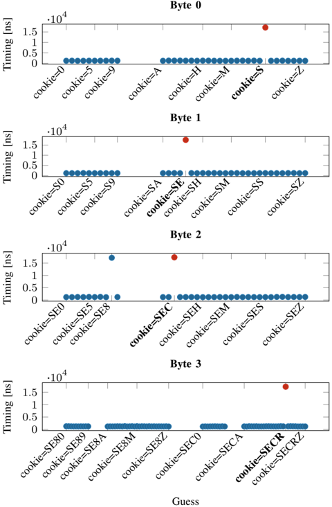<details> <summary>Image 12 Details</summary>  ### Visual Description ## Line Chart: Timing vs. Guess (Cookie Byte Analysis) ### Overview The image presents four separate line charts, arranged vertically. Each chart represents a different byte (Byte 0, Byte 1, Byte 2, Byte 3) and displays the relationship between "Timing" (in nanoseconds - ns) and a "Guess" value, which appears to be a cookie value. Each chart shows timing measurements for different cookie values. The x-axis represents the "Guess" (cookie value), and the y-axis represents "Timing" in nanoseconds. ### Components/Axes * **X-axis:** "Guess" - Represents the cookie value being tested. The values vary for each byte. * **Y-axis:** "Timing (ns)" - Represents the time taken, measured in nanoseconds. The scale ranges from 0 to 1.5 x 10⁴ ns (15,000 ns). * **Charts:** Four separate charts, one for each byte (0, 1, 2, 3). * **Data Points:** Each chart contains multiple data points, represented as blue triangles pointing downwards. There are also a few red circles in Byte 2 and Byte 3. * **Titles:** Each chart is labeled with "Byte X" (where X is 0, 1, 2, or 3). ### Detailed Analysis or Content Details **Byte 0:** * The line generally slopes downwards, indicating a decreasing timing with increasing cookie value. * cookie=0: Timing ≈ 1.45 x 10⁴ ns * cookie=5: Timing ≈ 1.1 x 10⁴ ns * cookie=9: Timing ≈ 0.8 x 10⁴ ns * cookie=A: Timing ≈ 0.6 x 10⁴ ns * cookie=H: Timing ≈ 0.5 x 10⁴ ns * cookie=M: Timing ≈ 0.4 x 10⁴ ns * cookie=S: Timing ≈ 0.3 x 10⁴ ns * cookie=Z: Timing ≈ 0.2 x 10⁴ ns **Byte 1:** * The line is relatively flat, with some fluctuations. * cookie=S0: Timing ≈ 1.4 x 10⁴ ns * cookie=S5: Timing ≈ 1.3 x 10⁴ ns * cookie=S9: Timing ≈ 1.2 x 10⁴ ns * cookie=SA: Timing ≈ 0.9 x 10⁴ ns * cookie=SE: Timing ≈ 0.7 x 10⁴ ns * cookie=SH: Timing ≈ 0.6 x 10⁴ ns * cookie=SM: Timing ≈ 0.5 x 10⁴ ns * cookie=SS: Timing ≈ 0.4 x 10⁴ ns * cookie=SZ: Timing ≈ 0.3 x 10⁴ ns **Byte 2:** * The line is mostly flat, with a few outliers. * cookie=SE0: Timing ≈ 1.4 x 10⁴ ns * cookie=SE5: Timing ≈ 1.3 x 10⁴ ns * cookie=SE8: Timing ≈ 1.2 x 10⁴ ns * cookie=SEC: Timing ≈ 0.8 x 10⁴ ns (Red circle) * cookie=SEH: Timing ≈ 0.7 x 10⁴ ns * cookie=SEM: Timing ≈ 0.6 x 10⁴ ns * cookie=SES: Timing ≈ 0.5 x 10⁴ ns * cookie=SEZ: Timing ≈ 0.4 x 10⁴ ns **Byte 3:** * The line is mostly flat, with a significant outlier. * cookie=SE80: Timing ≈ 1.4 x 10⁴ ns * cookie=SE89: Timing ≈ 1.3 x 10⁴ ns * cookie=SE8A: Timing ≈ 1.2 x 10⁴ ns * cookie=SE8M: Timing ≈ 1.1 x 10⁴ ns * cookie=SE8Z: Timing ≈ 0.9 x 10⁴ ns * cookie=SECO: Timing ≈ 0.7 x 10⁴ ns * cookie=SECR: Timing ≈ 0.6 x 10⁴ ns (Red circle) * cookie=SECRZ: Timing ≈ 0.5 x 10⁴ ns ### Key Observations * Byte 0 shows a clear negative correlation between the cookie value and timing. * Bytes 1, 2, and 3 exhibit relatively flat timing profiles, with some variations. * Bytes 2 and 3 have a few red data points that deviate significantly from the general trend. These could indicate anomalies or specific timing characteristics for those cookie values. * The timing values are generally high (above 10⁴ ns) and decrease as the cookie value increases. ### Interpretation The data suggests that the timing of some operation is sensitive to the value of the cookie, particularly in Byte 0. The decreasing timing with increasing cookie value in Byte 0 could indicate a caching or optimization mechanism that becomes more effective with higher cookie values. The relatively flat timing profiles in Bytes 1, 2, and 3 suggest that the timing is less sensitive to the cookie value in those bytes. The red data points in Bytes 2 and 3 could represent specific cookie values that trigger different code paths or require more processing time, leading to increased timing. The use of different cookie values (e.g., "S0", "SE8", "SECO") suggests that the cookie is composed of multiple parts or characters, and the timing is being measured for different combinations of these parts. The overall pattern suggests that the cookie is being used as an input to some timing-sensitive operation, and the goal of the measurements is to understand how the cookie value affects the performance of that operation. This could be related to security testing (e.g., timing attacks) or performance optimization. </details> Fig. 13: Median latency for ZRAM accesses in dictionary attack, with correct guess SECRET and 99 incorrect guesses (we only label 4 out of 99 incorrect guesses on X-axis for brevity). 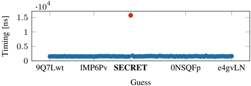<details> <summary>Image 13 Details</summary>  ### Visual Description \n ## Scatter Plot: Timing vs. Guess ### Overview The image presents a scatter plot visualizing the relationship between "Guess" and "Timing" (measured in nanoseconds). The plot shows a relatively flat distribution of timing values for most guesses, with a single significant outlier. ### Components/Axes * **X-axis:** "Guess" - Categorical variable with labels: 9Q7Lwt, IMP6Pv, SECRET, 0NSQFp, e4gvLN. * **Y-axis:** "Timing [ns]" - Numerical variable, scale ranging from 0 to 1.6 x 10⁴. * **Data Points:** Represented as small blue dots for most guesses, and a single red dot for the "SECRET" guess. ### Detailed Analysis The majority of data points cluster around a timing value of approximately 0.2 x 10⁴ ns (2000 ns). The data points for "9Q7Lwt", "IMP6Pv", "0NSQFp", and "e4gvLN" all fall within this range. The "SECRET" guess is represented by a single red data point located at approximately 1.55 x 10⁴ ns (15500 ns). This value is significantly higher than all other timing values observed in the plot. ### Key Observations * The timing values are consistent for all guesses except "SECRET". * The "SECRET" guess exhibits a substantially longer timing value, indicating a potential anomaly or difference in processing time. * The plot suggests a strong correlation between the "SECRET" guess and increased timing. ### Interpretation The data suggests that the "SECRET" guess requires significantly more time to process or execute compared to the other guesses. This could be due to a variety of factors, such as: * **Complexity:** The "SECRET" guess might involve a more complex calculation or operation. * **Resource Usage:** It could require more computational resources (CPU, memory, etc.). * **Security Measures:** The "SECRET" guess might trigger additional security checks or encryption/decryption processes. * **Cache Misses:** The data associated with "SECRET" might not be readily available in the cache, leading to slower access times. The outlier status of the "SECRET" guess warrants further investigation to understand the underlying cause of the timing difference. This could involve analyzing the code or process associated with the "SECRET" guess to identify performance bottlenecks or areas for optimization. The plot is a strong indicator of a potential issue or difference in behavior related to the "SECRET" guess. </details> of 100 possible guesses (dictionary), similar to previous PoCs. We assume the target page has a secret embedded the tophalf and the bottom half of the page is attacker-controlled and filled with repeated guesses from a dictionary. Figure 13 shows the median latency for attacker's data access from ZRAM (over 10 observations) for different guesses from the dictionary. The guesses consist of 99 randomly generated strings and the secret (cookie= SECRET ). We observe a high timing for decompression when the guess matches the secret as the page entropy is lowered (and the page compressed in ZRAM), thus leaking the secret; for all other guesses the decompression is fast. This dictionary attack completes in less than 10 minutes. But in general, the duration depends on the time required to force a target page into ZRAM, depending on the physical memory limit for a target process. Takeaway: We show that even if an application does not explicitly use compression, its data may still get compressed by the OS due to memory compression. Our case study of ZRAM shows that all compression algorithms in ZRAM have timing differences of 250 ns to 10 400 ns for accesses to compressed versus uncompressed pages. We also show that if secrets are co-located with attacker-controlled data in the same page and compressed with memory compression, they can be leaked in minutes. ## VII. MITIGATIONS Disabling LZ77. The most rudimentary solution is to completely disable compression or at least disable the LZ77 part. Karakostas et al. [31] showed for web pages that this adds an overhead between 91 % and 500 % . Furthermore, attacks have not been studied well enough on symbol compression to provide any security guarantees. Masking. Karakostas et al. [31] presented a generic defense technique called Context Transformation Extension (CTX). The general idea is to use context-hiding to protect secrets from being compressed with attacker-controlled data. Data is permuted on the server-side using a mask, and on the clientside, an inverse permutation is performed (JavaScript library). The overhead compared to the original algorithms decrease with the number of compressed data [31]. Randomization. Yang et al. [61] showed an approach with randomized input to mitigate compression side-channel attacks. The service would require adding an additional amount of random data to hide the size of the compressed memory. However, as the authors also show, randomization-based approaches can be defeated with at the expense of a higher execution time. Also, Karaskostas et al. [31] showed that size randomization is ineffective against memory compression attacks. It is also unclear if size randomization mitigates the timing-based side channel of the memory decompression. Keyword protection. Zieli´ nski demonstrated an implementation of DEFLATE called SafeDeflate [66]. SafeDeflate mitigates memory compression attacks by splitting the set of keywords into subsets of sensitive and non-sensitive keywords. Depending on the completeness of the sensitive keyword list, this approach can be considered as secure, but there is no guaranteed security. As Paulsen et al. [43] mention, it is easy to overlook a corner case. Furthermore, this approach leads to a loss of compression ratio of about 200 % to 400 % [31]. Taint tracking. Taint tracking tries to trace the data flow and mark input sources and their sinks. Paulsen et al. [43] use taint analysis to track the flow of secret data before feeding data into the compression algorithm. Their tool, Debreach, is about 2-5 times faster than SafeDeflate [43]. However, this approach is, so far, only compatible with PHP. Furthermore, for such an approach, the developer needs to flag the sensitive input which is being tracked. The probably best strategy in practice is to avoid sensitive data being compressed with potential attacker-controlled data. The aforementioned mitigations focus on mitigating compression ratio side channels. As the compression and decompression timings are not constant, a timing side channel is harder to mitigate, e.g., remote attacks might be mitigated by adding artificial noise or using network packet inspection to detect attacks [52]. Since the latency for a correct guess is in the region of microseconds, not many requests ( & 200 ) are required per guess to distinguish the latency. Therefore a simple DDoS detection might detect an attack but only after a certain amount of data being leaked. ## VIII. CONCLUSION In this paper, we presented a timing side channel attack on several memory compression algorithms. With Comprezzor, we developed a generic approach to amplify latencies for correct guesses when performing dictionary attack on different compression algorithms. Our remote covert channel achieves a transmission rate of 643 . 25 bit ♥ h over 14 hops in the internet. We demonstrated three cases studies on memory compression attacks. First, we showed a remote dictionary attack on a PHP application, hosted on an Nginx, storing zlibcompressed data in Memcached. We demonstrate bytewise leakage across the internet from a server located 14 hops away. Using Comprezzor, we explored high timing differences when performing a dictionary attack on PostgreSQLs PGLZ algorithm. and leveraged those to leak database records from PostgreSQL. Lastly, we also demonstrated a dictionary attack on ZRAM. ## REFERENCES - [1] Acıic ¸mez, Onur and Schindler, Werner and Koc, Cetin K. Cache based remote timing attack on the aes. In CT-RSA , 2006. - [2] Hassan Aly and Mohammed ElGayyar. Attacking aes using bernstein's attack on modern processors. In International Conference on Cryptology in Africa , 2013. - [3] Apple Insider, 2013. URL: https://appleinsider.com/articles/13/06/13/c ompressed-memory-in-os-x-109-mavericks-aims-to-free-ram-extendbattery-life. - [4] Tal Be'ery and Amichai Shulman. A Perfect CRIME? Only TIME Will Tell. Black Hat Europe , 2013. - [5] Bmemcached. bmemcached package, 2021. URL: https://python-binarymemcached.readthedocs.io/en/latest/bmemcached/. - [6] BTRFS. Compression, 2021. URL: https://btrfs.wiki.kernel.org/index. php/Compression#Why does not du report the compressed size.3F. - [7] Buckenhofer. PostgreSQL Columnar Storage, 2021. URL: https://www. buckenhofer.com/2021/01/postgresql-columnar-extension-cstore/. - [8] Euccas Chen. Understanding zlib, 2021. URL: https://www.euccas.me/ zlib/#deflate. - [9] Citus. Columnar: Distributed PostgreSQL as an extension., 2021. URL: https://github.com/citusdata/citus/blob/master/src/backend/columnar/RE ADME.md. - [10] Collett, Yann. Smaller and faster data compression with Zstandard, 2016. URL: https://engineering.fb.com/2016/08/31/core-data/smaller-andfaster-data-compression-with-zstandard/. - [11] DennyL. Enabling ZRAM in Chrome OS, 2020. URL: https://suppor t.google.com/chromebook/thread/75256850/enabeling-zram-doesn-twork-in-crosh?hl=en&msgid=75453860. - [12] P. Deutsch. Rfc1951: Deflate compressed data format specification version 1.3, 1996. - [13] Equinix, 2021. URL: https://www.packet.com/. - [14] Dmitry Evtyushkin and Dmitry Ponomarev. Covert channels through random number generator: Mechanisms, capacity estimation and mitigations. In CCS , 2016. - [15] R. Fielding, J. Gettys, J. Mogul, H. Frystyk, L. Masinter, P. Leach, and T. Berners-Lee. Rfc 2616, hypertext transfer protocol - http/1.1, 1999. URL: http://www.rfc.net/rfc2616.html. - [16] Andrea Fioraldi, Dominik Maier, Heiko Eißfeldt, and Marc Heuse. AFL++: Combining incremental steps of fuzzing research. In USENIX Workshop on Offensive Technologies (WOOT) , August 2020. - [17] Flask. Flask, 2021. URL: https://flask.palletsprojects.com/en/2.0.x/. - [18] Anders Fogh. Covert Shotgun: automatically finding SMT covert channels, 2016. URL: https://cyber.wtf/2016/09/27/covert-shotgun/. - [19] Gailly, Jean-loup and Adler, Mark. zlib.h - interface of the 'zlib' general purpose compression library, 2020. URL: https://github.com/torvalds/li nux/blob/5bfc75d92efd494db37f5c4c173d3639d4772966/include/linux/ zlib.h. - [20] Yoel Gluck, Neal Harris, and Angelo Prado. BREACH: reviving the CRIME attack. Unpublished manuscript , 2013. - [21] Ben Gras, Cristiano Giuffrida, Michael Kurth, Herbert Bos, and Kaveh Razavi. ABSynthe: Automatic Blackbox Side-channel Synthesis on Commodity Microarchitectures. In NDSS , 2020. - [22] Daniel Gruss, Erik Kraft, Trishita Tiwari, Michael Schwarz, Ari Trachtenberg, Jason Hennessey, Alex Ionescu, and Anders Fogh. Page Cache Attacks. In CCS , 2019. - [23] Daniel Gruss, Cl´ ementine Maurice, Klaus Wagner, and Stefan Mangard. Flush+Flush: A Fast and Stealthy Cache Attack. In DIMVA , 2016. - [24] Daniel Gruss, Raphael Spreitzer, and Stefan Mangard. Cache Template Attacks: Automating Attacks on Inclusive Last-Level Caches. In USENIX Security Symposium , 2015. - [25] Berk G¨ ulmezo˘ glu, Mehmet Sinan Inci, Thomas Eisenbarth, and Berk Sunar. A Faster and More Realistic Flush+Reload Attack on AES. In COSADE , 2015. - [26] Gupta, Nitin. zram: Compressed RAM-based block devices, 2021. URL: https://www.kernel.org/doc/html/latest/admin-guide/blockdev/zram.ht ml. - [27] Shaobo He, Michael Emmi, and Gabriela Ciocarlie. ct-fuzz: Fuzzing for timing leaks. In International Conference on Software Testing, Validation and Verification (ICST) , 2020. doi:10.1109/ICST46399.2020 .00063 . - [28] Hoffman, Chris. What Is Memory Compression in Windows 10?, 2017. URL: https://www.howtogeek.com/319933/what-is-memory-compressio n-in-windows-10/. - [29] holmeshe.me. Understanding the memcached source code - slab ii, 2020. URL: https://holmeshe.me/understanding-memcached-source-code-II/. - [30] Darshana Jayasinghe, Jayani Fernando, Ranil Herath, and Roshan Ragel. Remote cache timing attack on advanced encryption standard and countermeasures. In ICIAFs , 2010. - [31] Dimitris Karakostas, Aggelos Kiayias, Eva Sarafianou, and Dionysis Zindros. Ctx: Eliminating breach with context hiding. Black Hat EU , 2016. - [32] Dimitris Karakostas and Dionysis Zindros. Practical new developments on breach. Black Hat Asia , 2016. - [33] John Kelsey. Compression and information leakage of plaintext. In Fast Software Encryption , 2002. - [34] Larabel, Michael. What Is Memory Compression in Windows 10?, 2020. URL: https://www.phoronix.com/scan.php?page=news item&px=Fedo ra-33-Swap-On-zRAM-Proposal. - [35] Moritz Lipp, Daniel Gruss, Raphael Spreitzer, Cl´ ementine Maurice, and Stefan Mangard. ARMageddon: Cache Attacks on Mobile Devices. In USENIX Security Symposium , 2016. - [36] Fangfei Liu, Yuval Yarom, Qian Ge, Gernot Heiser, and Ruby B. Lee. Last-Level Cache Side-Channel Attacks are Practical. In S&P , 2015. - [37] Cl´ ementine Maurice, Manuel Weber, Michael Schwarz, Lukas Giner, Daniel Gruss, Carlo Alberto Boano, Stefan Mangard, and Kay R¨ omer. Hello from the Other Side: SSH over Robust Cache Covert Channels in the Cloud. In NDSS , 2017. - [38] Memcached, 2020. URL: https://memcached.org/. - [39] Microsoft. concepts-hyperscale-columnar, 2021. URL: https://docs.mic rosoft.com/en-us/azure/postgresql/concepts-hyperscale-columnar. - [40] Daniel Moghimi, Moritz Lipp, Berk Sunar, and Michael Schwarz. Medusa: Microarchitectural Data Leakage via Automated Attack Synthesis. In USENIX Security Symposium , 2020. - [41] Mozilla. Compression in HTTP, 2021. URL: https://developer.mozilla. org/en-US/docs/Web/HTTP/Compression. - [42] Shirin Nilizadeh, Yannic Noller, and Corina S Pasareanu. Diffuzz: differential fuzzing for side-channel analysis. In International Conference on Software Engineering (ICSE) , 2019. - [43] Brandon Paulsen, Chungha Sung, Peter AH Peterson, and Chao Wang. Debreach: mitigating compression side channels via static analysis and transformation. In IEEE/ACM International Conference on Automated Software Engineering (ASE) . IEEE, 2019. - [44] Peter Pessl, Daniel Gruss, Cl´ ementine Maurice, Michael Schwarz, and Stefan Mangard. DRAMA: Exploiting DRAM Addressing for CrossCPU Attacks. In USENIX Security Symposium , 2016. - [45] php.net. memcached.constants.php, 2021. URL: https://www.php.net/ manual/en/memcached.constants.php. - [46] PostgreSQL. TOAST Compression, 2021. URL: https://www.postgresql .org/docs/current/storage-toast.html. - [47] Hany Ragab, Alyssa Milburn, Kaveh Razavi, Herbert Bos, and Cristiano Giuffrida. CrossTalk: Speculative Data Leaks Across Cores Are Real. In S&P , 2021. - [48] Sanjay Rawat, Vivek Jain, Ashish Kumar, Lucian Cojocar, Cristiano Giuffrida, and Herbert Bos. Vuzzer: Application-aware evolutionary fuzzing. In NDSS , 2017. - [49] Juliano Rizzo and Thai Duong. The CRIME attack. In ekoparty security conference , volume 2012, 2012. - [50] Rostedt, Steven. ftrace - Function Tracer, 2017. URL: https://www.kern el.org/doc/Documentation/trace/ftrace.txt. - [51] Vishal Saraswat, Daniel Feldman, Denis Foo Kune, and Satyajit Das. Remote cache-timing attacks against aes. In Workshop on Cryptography and Security in Computing Systems , 2014. - [52] Michael Schwarz, Martin Schwarzl, Moritz Lipp, and Daniel Gruss. NetSpectre: Read Arbitrary Memory over Network. In ESORICS , 2019. - [53] Benjamin Semal, Konstantinos Markantonakis, Keith Mayes, and Jan Kalbantner. One covert channel to rule them all: A practical approach to data exfiltration in the cloud. In IEEE International Conference on Trust, Security and Privacy in Computing and Communications (TrustCom) , 2020. - [54] Dongdong She, Kexin Pei, Dave Epstein, Junfeng Yang, Baishakhi Ray, and Suman Jana. Neuzz: Efficient fuzzing with neural program smoothing. In IEEE Symposium on Security and Privacy , 2019. doi: 10.1109/SP.2019.00052 . - [55] Po-An Tsai, Andres Sanchez, Christopher W. Fletcher, and Daniel Sanchez. Safecracker: Leaking secrets through compressed caches. In ASPLOS , 2020. - [56] Tom Van Goethem, Christina P¨ opper, Wouter Joosen, and Mathy Vanhoef. Timeless Timing Attacks: Exploiting Concurrency to Leak Secrets over Remote Connections. In USENIX Security Symposium , 2020. - [57] Tom Van Goethem, Mathy Vanhoef, Frank Piessens, and Wouter Joosen. Request and conquer: Exposing cross-origin resource size. In USENIX Security Symposium , 2016. - [58] Mathy Vanhoef and Tom Van Goethem. Heist: Http encrypted information can be stolen through tcp-windows. In Black Hat US Briefings, Location: Las Vegas, USA , 2016. - [59] Daniel Weber, Ahmad Ibrahim, Hamed Nemati, Michael Schwarz, and Christian Rossow. Osiris: Automated Discovery Of Microarchitectural Side Channels. In USENIX Security Symposium , 2021. - [60] Zhenyu Wu, Zhang Xu, and Haining Wang. Whispers in the Hyperspace: High-speed Covert Channel Attacks in the Cloud. In USENIX Security Symposium , 2012. - [61] Meng Yang and Guang Gong. Lempel-ziv compression with randomized input-output for anti-compression side-channel attacks under https/tls. In International Symposium on Foundations and Practice of Security . Springer, 2019. - [62] Yuval Yarom and Katrina Falkner. Flush+Reload: a High Resolution, Low Noise, L3 Cache Side-Channel Attack. In USENIX Security Symposium , 2014. - [63] Pavel Yosifovich, Alex Ionescu, Mark E. Russinovich, and David A. Solomon. Windows Internals Part 1 . Microsoft Press, 7 edition, 2017. - [64] Michał Zalewski. American Fuzzy Lop, 2021. URL: https://github.com /Google/AFL. - [65] Xin-jie Zhao, Tao Wang, and Yuanyuan Zheng. Cache Timing Attacks on Camellia Block Cipher. Cryptology ePrint Archive, Report 2009/354 , 2009. - [66] Michał Zielinski. Safedeflate: compression without leaking secrets. Technical report, Cryptology ePrint Archive, Report 2016/958. 2016, 2016. ## APPENDIX A TIMING DIFFERENCE FOR COMPRESSION TABLE IV: Different compression algorithms yield distinguishable timing differences when compressing content with a different entropy. ( n 100000 | Algorithm | Fully Compressible (ns) | Partially Compressible (ns) | Incompressible (ns) | |-----------------------------------|------------------------------------------------------------------------------------------------------------------------------------------------------------------------------------------------------------------------------------|-------------------------------------------------------------------------------------------------------------------------------------------------------------------------------------------------------------------------------------|------------------------------------------------------------------------------------------------------------------------------------------------------------------------------------------------------| | FastLZ LZ4 LZ4 LZO PGLZ zlib zstd | 38619 . 07 ( 0 . 74% ) 606 . 82 ( 0 . 93% ) 44748 . 02 ( 0 . 15% ) 5645 . 86 ( 2 . 18% ) 44275 . 84 ( 0 . 13% ) 38479 . 53 ( 0 . 22% ) 3596 . 41 ( 0 . 42% ) | 58887 . 40 ( 0 . 50% ) 220 . 63 ( 1 . 00% ) 47731 . 08 ( 0 . 16% ) 5915 . 28 ( 2 . 78% ) 65752 . 55 ( 0 . 12% ) 80284 . 72 ( 0 . 23% ) 22288 . 14 ( 0 . 52% ) | 79384 . 89 ( 0 . 40% ) 231 . 76 ( 1 . 97% ) 47316 . 56 ( 0 . 16% ) 7928 . 21 ( 3 . 91% ) - 76973 . 82 ( 0 . 20% ) 29284 . 77 ( 0 . 34% ) | ## APPENDIX B KERNEL TRACE FOR ZRAM DECOMPRESSION To highlight the root-cause of the timing differences in ZRAM accesses, we trace the kernel functions called on accesses to ZRAM pages using the ftrace [50] utility. Listing 1 and Listing 2 show the trace of kernel functions called on an access to an incompressible and compressible page respectively in ZRAM (using deflate algorithm). The incompressible page contains random bytes, while the compressible page contains 2048 bytes of the same value and 2048 random bytes similar to the partially-compressible setting in Section VI-E1. We only show the functions which are called when the ZRAM page is swapped in to regular memory. The main difference between the two listings (colored in red) is that the functions performing decompression of the ZRAM page are only called when a compressible page is swapped-in, while these functions are skipped for the page stored uncompressed. Of these additional function calls, the main driver of the timing difference is the \_\_deflate\_decompress function in Listing 2 which consumes 12555 ns. This ties in with the characterization study in Section VI-E1 which showed the average timing difference between accesses to compressible and incompressible pages to be close to 10000 ns for ZRAM with deflate algorithm. These timings are for the deflate implementation in the Linux kernel, which is a modified version of zlib v1.1.3 [19]; hence these timings differ from the zlib timings measured in Table I for the more recent zlib v1.2.11 . Listing 1: Kernel function trace for ZRAM access to incompressible page <details> <summary>Image 14 Details</summary>  ### Visual Description ## Data Table: Function Call Timings ### Overview The image presents a data table listing function names and their corresponding execution times in nanoseconds (ns). The table appears to represent a sequence of function calls and their timings, potentially during a system operation or profiling session. ### Components/Axes The table has two columns: * **Time (ns)**: Represents the execution time of the function, measured in nanoseconds. The values are listed in ascending order. * **Function**: Represents the name of the function being called. The table is numbered from 1 to 23, indicating the sequence of function calls. ### Detailed Analysis / Content Details Here's a reconstruction of the data table content: | Row | Time (ns) | Function | |-----|-----------|-----------------------| | 1 | 0 | swap_readpage | | 2 | 62 | page_swap_info | | 3 | 126 | \_frontswap_load | | 4 | 195 | \_page_file_index | | 5 | 254 | bdev_read_page | | 6 | 326 | blk_queue_enter | | 7 | 395 | zram_rw_page | | 8 | 460 | zram_bvec_rw.isra.0 | | 9 | 527 | generic_start_io_acct | | 10 | 590 | update_io_ticks | | 11 | 661 | part_inc_in_flight | | 12 | 729 | \_zram_bvec_read.constprop.0 | | 13 | 813 | zs_map_object | | 14 | 967 | \_raw_read_lock | | 15 | 1407 | zs_unmap_object | | 16 | 1487 | generic_end_io_acct | | 17 | 1550 | update_io_ticks | | 18 | 1617 | jiffies_to_usecs | | 19 | 1677 | part_dec_in_flight | | 20 | 1753 | ktime_get_with_offset| | 21 | 1835 | page_endio | | 22 | 1904 | unlock_page | The time values increase monotonically, indicating a sequential execution of the functions. The time differences between consecutive function calls vary, suggesting differing execution complexities. ### Key Observations * The function `update_io_ticks` appears twice in the list, at times 590 ns and 1550 ns. * The largest time difference between consecutive function calls is between `\_raw_read_lock` (967 ns) and `zs_unmap_object` (1407 ns), indicating a potentially long-running operation or a significant delay. * The initial function calls (`swap_readpage`, `page_swap_info`, etc.) have relatively small time differences, while later calls exhibit larger differences. ### Interpretation This data likely represents a performance trace of a system operation involving page swapping, block device access, and memory management. The functions listed suggest operations related to virtual memory, disk I/O, and potentially compression (zram). The timings provide insights into the performance characteristics of these operations. The repeated call to `update_io_ticks` suggests a periodic task related to I/O accounting. The large time difference before `zs_unmap_object` could indicate a blocking operation or a significant amount of processing within `\_raw_read_lock`. Analyzing these timings could help identify performance bottlenecks and optimize the system for faster operation. The data could be used to understand the overhead associated with different system calls and to prioritize optimization efforts. The sequence of function calls also provides a high-level view of the system's activity during the traced period. 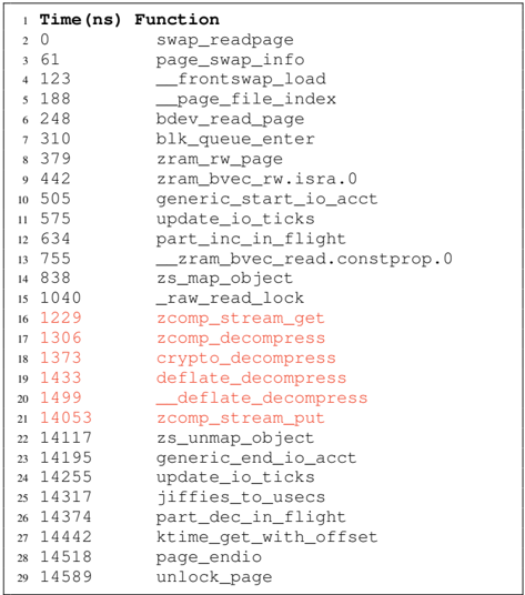</details> Listing 2: Kernel function trace for ZRAM access to compressible page <details> <summary>Image 15 Details</summary>  ### Visual Description \n ## Data Table: Function Call Timings ### Overview The image presents a data table listing function call timings in nanoseconds (ns). The table appears to represent a trace or profiling data, showing the execution time of various functions. ### Components/Axes The table has two columns: * **Time (ns)**: Represents the elapsed time in nanoseconds, starting from 0 and increasing to 14589. * **Function**: Lists the names of the functions being timed. The table is numbered from 1 to 29, indicating the sequence of function calls. ### Detailed Analysis or Content Details Here's a reconstruction of the data table content: | # | Time (ns) | Function | | --- | --------- | ----------------------- | | 1 | 0 | swap_readpage | | 2 | 61 | page_swap_info | | 3 | 123 | _frontswap_load | | 4 | 188 | _page_file_index | | 5 | 248 | bdev_read_page | | 6 | 310 | blk_queue_enter | | 7 | 379 | zram_rw_page | | 8 | 442 | zram_bvec_rw.isra.0 | | 9 | 505 | generic_start_io_acct | | 10 | 575 | update_io_ticks | | 11 | 634 | part_inc_in_flight | | 12 | 755 | _zram_bvec_read.constprop.0 | | 13 | 838 | zs_map_object | | 14 | 1040 | _raw_read_lock | | 15 | 1229 | zcomp_stream_get | | 16 | 1306 | zcomp_decompress | | 17 | 1373 | crypto_decompress | | 18 | 1433 | deflate_decompress | | 19 | 1499 | _deflate_decompress | | 20 | 14053 | zcomp_stream_put | | 21 | 14117 | zs_unmap_object | | 22 | 14195 | generic_end_io_acct | | 23 | 14255 | update_io_ticks | | 24 | 14317 | jiffies_to_usecs | | 25 | 14374 | part_dec_in_flight | | 26 | 14442 | ktime_get_with_offset | | 27 | 14518 | page_endio | | 28 | 14589 | unlock_page | ### Key Observations * The function timings are not evenly distributed. There are clusters of functions with relatively small timings (e.g., lines 1-12), followed by a jump to larger timings (lines 20-28). * `update_io_ticks` appears twice in the list (lines 10 and 23), suggesting it's called multiple times during the traced operation. * The functions starting with an underscore (`_`) likely represent internal or compiler-optimized functions. * The functions related to compression (`zcomp_stream_get`, `zcomp_decompress`, `crypto_decompress`, `deflate_decompress`) have relatively high timings compared to the initial functions. ### Interpretation This data table likely represents a performance trace of a system operation involving disk I/O, memory management, and data compression. The initial functions (lines 1-12) seem to be related to setting up and initiating the I/O operation. The compression-related functions (lines 16-19) indicate that data is being compressed during the process, which is computationally expensive. The later functions (lines 20-28) likely represent the completion and cleanup phases of the operation. The repeated call to `update_io_ticks` suggests that I/O statistics are being updated periodically. The large jump in timings between lines 12 and 20 could indicate a significant operation, such as reading a large block of data from disk or performing a complex compression algorithm. The data suggests that the compression stage is a performance bottleneck in this operation. Further analysis could involve identifying the specific data being compressed and optimizing the compression algorithm or reducing the amount of data that needs to be compressed. The presence of functions with `.isra.0` and `.constprop.0` suffixes suggests that the code has been optimized using compiler techniques like interprocedural scalar replacement aggregation (ISRA) and constant propagation. </details> ## APPENDIX C ## LAYOUT DISCOVERED BY COMPREZZOR Figure 14 shows the layout discovered by the Comprezzor that amplifies the timing difference for decompression of the correct and incorrect guesses in Zlib dictionary attack. Listing 3 and Listing 4 show the debug trace from the Zlib code for decompression with the correct and incorrect guesses to illustrate the root cause of the timing differences. Fig. 14: Incorrect guesses with the corner-case discovered by Comprezzor lead to a dynamic Huffman block creation for the partially compressible data, that is slow to decompress. 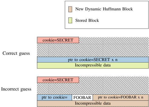<details> <summary>Image 16 Details</summary>  ### Visual Description \n ## Diagram: Cookie Guessing Illustration ### Overview The image is a diagram illustrating the difference between a correct and incorrect guess in a cookie-based system, likely related to data compression or security. It depicts two scenarios: one where the cookie guess is correct and one where it is incorrect, showing how data is stored and accessed in each case. The diagram uses colored blocks to represent different data segments and labels to identify their content. ### Components/Axes The diagram consists of two main sections, labeled "Correct guess" and "Incorrect guess", stacked vertically. Each section contains a series of rectangular blocks representing data storage. A legend is present in the top-right corner, defining the colors used: * Light Beige: "New Dynamic Huffman Block" * Light Green: "Stored Block" * Blue: "ptr to cookie=SECRET x n" * Red: "cookie=SECRET" * Orange: "ptr to cookie=FOOBAR x n" * Yellow: "Incompressible data" ### Detailed Analysis or Content Details **Correct Guess:** * The top layer is a large block filled with diagonal lines, representing the "New Dynamic Huffman Block". * Below this is a red block labeled "cookie=SECRET". * Beneath the red block is a blue block labeled "ptr to cookie=SECRET x n". * Finally, at the bottom, is a yellow block labeled "Incompressible data". **Incorrect Guess:** * The top layer is a large block filled with diagonal lines, representing the "New Dynamic Huffman Block". * Below this is a red block labeled "cookie=SECRET". * Beneath the red block are two blocks: a blue block labeled "ptr to cookie=FOOBAR" and another blue block labeled "ptr to cookie=FOOBAR x n". * Finally, at the bottom, is an orange block labeled "Incompressible data". ### Key Observations * The key difference between the two scenarios is the value of the pointer ("ptr to cookie") and the associated data. In the correct guess, the pointer points to "SECRET", while in the incorrect guess, it points to "FOOBAR". * The "Incompressible data" is yellow in the correct guess and orange in the incorrect guess, suggesting a change in data type or storage location based on the guess. * The "cookie=SECRET" block remains consistent in both scenarios. ### Interpretation This diagram illustrates a security or data integrity mechanism where a "cookie" value is used to validate data access. The "cookie=SECRET" likely represents a valid authentication token or key. The "ptr to cookie" acts as a pointer to the correct data location. * **Correct Guess:** When the guess is correct (pointer points to "SECRET"), the system successfully retrieves the "Incompressible data" (yellow). This suggests a successful authentication or data validation. * **Incorrect Guess:** When the guess is incorrect (pointer points to "FOOBAR"), the system retrieves different data ("Incompressible data" is orange). This indicates a failed authentication or data validation, potentially leading to access to incorrect or decoy data. The "New Dynamic Huffman Block" likely represents a compression or encoding scheme used to store the data. The diagram highlights how an incorrect guess can lead to accessing different data, potentially revealing information about the system's security mechanisms or data structure. The use of "FOOBAR" as a decoy value is a common practice in security testing and demonstrates a deliberate attempt to mislead an attacker. The diagram suggests a system where data integrity relies on the correct "cookie" value and its associated pointer. </details> Listing 3: Trace for correct guess in zlib. Here the entire guess string is compressed and the remainder is incompressible (decompressed fast as a stored block). 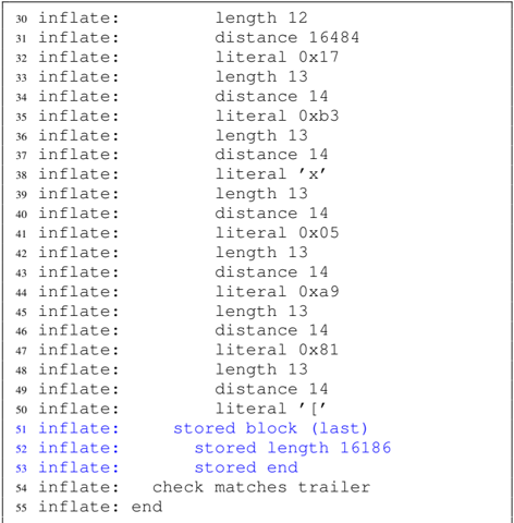<details> <summary>Image 17 Details</summary>  ### Visual Description \n ## Text Block: Inflate Sequence ### Overview The image presents a sequence of lines, each starting with "inflate:" followed by a description of an operation or data. This appears to be a log or trace of a decompression process, likely using the DEFLATE algorithm (commonly used in zlib). The lines detail length, distance, and literal values used during the inflation process. ### Components/Axes There are no axes or traditional components like in a chart. The data is presented as a sequential list. The first column is a line number (30-55). The second column is the operation "inflate:". The third column contains the details of the operation. ### Detailed Analysis or Content Details Here's a transcription of the content, line by line: * 30 inflate: length 12 * 31 inflate: distance 16484 * 32 inflate: literal 0x17 * 33 inflate: length 13 * 34 inflate: distance 14 * 35 inflate: literal 0xb3 * 36 inflate: length 13 * 37 inflate: distance 14 * 38 inflate: literal 'x' * 39 inflate: length 13 * 40 inflate: distance 14 * 41 inflate: literal 0x05 * 42 inflate: length 13 * 43 inflate: distance 14 * 44 inflate: literal 0xa9 * 45 inflate: length 13 * 46 inflate: distance 14 * 47 inflate: literal 0x81 * 48 inflate: length 13 * 49 inflate: distance 14 * 50 inflate: literal '[' * 51 inflate: stored block (last) * 52 inflate: stored length 16186 * 53 inflate: stored end * 54 inflate: check matches trailer * 55 inflate: end ### Key Observations The sequence shows repeated patterns of "length" and "distance" pairs, interspersed with "literal" values. The "literal" values include hexadecimal representations (e.g., 0x17, 0xb3) and a character ('x', '['). The final lines indicate the end of a stored block and a successful check of the trailer, signifying the completion of the decompression process. The distance values are significantly larger in the beginning (16484) and then consistently 14. ### Interpretation This data represents the steps taken during the decompression of a data stream using the DEFLATE algorithm. The "length" and "distance" values likely refer to repeated sequences within the compressed data, allowing for efficient storage. The "literal" values represent unique bytes that are not part of a repeated sequence. The sequence suggests that the compressed data contained a large initial repeated sequence (distance 16484), followed by a series of shorter repeated sequences (distance 14). The "stored block (last)" indicates that a portion of the decompressed data was stored directly without further compression. The "check matches trailer" confirms the integrity of the decompressed data. This log provides a detailed view into the inner workings of the DEFLATE decompression process. </details> Listing 4: Trace for incorrect guess in zlib. Here only part of the guess string ( cookie= ) is compressed and the remainder cookie=FOOBAR is separately compressed (decompression requires a slower code block for Huffman tree decoding). 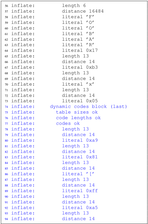<details> <summary>Image 18 Details</summary>  ### Visual Description ## Textual Data: Inflate Sequence Log ### Overview The image presents a log of an "inflate" process, likely related to data compression/decompression (e.g., zlib). It consists of numbered lines, each detailing an operation or data element encountered during the inflation process. The log entries primarily consist of the keyword "inflate:", followed by either a "length" value, a "distance" value, or a "literal" value (often represented in hexadecimal). There are also a few descriptive messages indicating the completion of a block and status checks. ### Components/Axes There are no axes or traditional chart components. The data is presented as a sequential list. The primary components are: * **Line Number:** Integers from 56 to 94, indicating the sequence of operations. * **Operation:** The keyword "inflate:". * **Parameter:** The value associated with the "inflate:" operation, which can be: * "length" followed by an integer value. * "distance" followed by an integer value. * "literal" followed by a character or hexadecimal value. * Descriptive text messages (e.g., "dynamic codes block (last)", "table sizes ok"). ### Detailed Analysis / Content Details Here's a transcription of the log entries, with approximate values: * 56 inflate: length 6 * 57 inflate: distance 16484 * 58 inflate: literal 'F' * 59 inflate: literal 'O' * 60 inflate: literal 'O' * 61 inflate: literal 'B' * 62 inflate: literal 'A' * 63 inflate: literal 'R' * 64 inflate: literal 0x17 * 65 inflate: length 13 * 66 inflate: distance 14 * 67 inflate: literal 0xb3 * 68 inflate: length 13 * 69 inflate: distance 14 * 70 inflate: literal 'x' * 71 inflate: length 13 * 72 inflate: distance 14 * 73 inflate: literal 0x05 * 74 inflate: dynamic codes block (last) * 75 inflate: table sizes ok * 76 inflate: code lengths ok * 77 inflate: codes ok * 78 inflate: length 13 * 79 inflate: distance 14 * 80 inflate: literal 0xa9 * 81 inflate: length 13 * 82 inflate: distance 14 * 83 inflate: literal 0x81 * 84 inflate: length 13 * 85 inflate: distance 14 * 86 inflate: literal '[' * 87 inflate: length 13 * 88 inflate: distance 14 * 89 inflate: literal 0xff * 90 inflate: length 13 * 91 inflate: distance 14 * 92 inflate: literal 0xa5 * 93 inflate: length 13 * 94 inflate: distance 14 ### Key Observations * The log shows a repeating pattern of "length", "distance", and "literal" operations. * The "distance" values are consistently 14 for a significant portion of the log (lines 66-73, 78-94). * The "length" values are consistently 13 for a significant portion of the log (lines 65, 68, 71, 78, 81, 84, 87, 90, 93). * The "literal" values include both ASCII characters (e.g., 'F', 'O', 'B', 'A', 'R', 'x', '[') and hexadecimal representations (e.g., 0x17, 0xb3, 0x05, 0xa9, 0x81, 0xff, 0xa5). * Lines 74-77 indicate the successful initialization of dynamic Huffman codes. ### Interpretation This log likely represents the decompression of a data stream using a compression algorithm like zlib. The "length" and "distance" values are used for LZ77-style compression, where repeated sequences of data are replaced with a length and a distance back to a previous occurrence. The "literal" values represent the actual data bytes. The consistent "distance" and "length" values suggest that the compressed data contains many repeated sequences. The "dynamic codes block (last)" message indicates that the Huffman coding tables were dynamically generated and are now finalized. The log provides a detailed trace of the decompression process, which could be useful for debugging or analyzing the compression algorithm's performance. The presence of both ASCII characters and hexadecimal values in the "literal" fields suggests that the original data stream contained a mix of text and binary data. </details> ## APPENDIX D BYTEWISE LEAKAGE Figure 15 illustrates the bytewise leakage of the secret (SECRET) for a PHP application using PHP-Memcached. Figure 16 shows the bytewise of the secret string for a Flask application that stores secret data together with attackercontrolled data into PostgreSQL. The prefix value can be shifted bytewise, which allows reusing the same memory layouts found by Comprezzor. Figure 17 shows the last two bytes leaked from a secret (SECRET) in a ZRAM page. This is a continuation of Figure 12 which showed the leakage of the first four bytes. Fig. 15: Bytewise leakage of the secret (S,E,C,R,E,T) from PHP-Memcached. In each plot, the lowest timing (shown in red) indicates the correct guess. 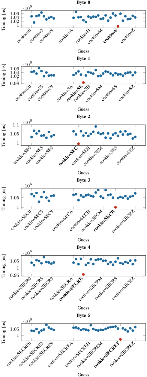<details> <summary>Image 19 Details</summary>  ### Visual Description ## Scatter Plots: Timing vs. Guess for Cookie Bytes ### Overview The image presents six separate scatter plots, each representing the timing (in nanoseconds) required to guess a specific byte of a "cookie". Each plot focuses on a different byte (Byte 0 through Byte 5). The x-axis represents the "Guess" (possible values for the byte), and the y-axis represents the "Timing" (in nanoseconds). Each plot displays data points for various guesses, with the color of the points varying between plots. ### Components/Axes * **Title:** Each plot is labeled with "Byte [Number]" (0-5) at the top-right corner. * **X-axis:** "Guess" - Categorical values representing possible byte values. The values are: * Byte 0: cookie=0, cookie=5, cookie=9, cookie=A, cookie=H, cookie=M, cookie=S, cookie=Z * Byte 1: cookie=S0, cookie=S5, cookie=S9, cookie=SA, cookie=SE, cookie=SH, cookie=SM, cookie=SS, cookie=SZ * Byte 2: cookie=SE0, cookie=SE5, cookie=SE9, cookie=SEC, cookie=SEH, cookie=SEM, cookie=SES, cookie=SEZ * Byte 3: cookie=SEC0, cookie=SEC5, cookie=SEC9, cookie=SECA, cookie=SECH, cookie=SECM, cookie=SECR, cookie=SECZ * Byte 4: cookie=SECR0, cookie=SECR5, cookie=SECR9, cookie=SECRA, cookie=SECRE, cookie=SECRM, cookie=SECRS, cookie=SECRZ * Byte 5: cookie=SECRED, cookie=SECRE5, cookie=SECRE9, cookie=SECREA, cookie=SECREH, cookie=SECREM, cookie=SECRES, cookie=SECREZ * **Y-axis:** "Timing (ns)" - Scale ranges from approximately 0.98 x 10⁶ to 1.1 x 10⁶ nanoseconds. * **Data Points:** Scatter points representing the timing for each guess. * **Colors:** Each byte plot uses a distinct color for its data points: * Byte 0: Blue * Byte 1: Orange * Byte 2: Purple * Byte 3: Red * Byte 4: Green * Byte 5: Teal ### Detailed Analysis or Content Details **Byte 0 (Blue):** The timing appears relatively constant across all guesses, hovering around 1.03 x 10⁶ ns. There's minimal variation. * Approximate values: ~1.03 x 10⁶ ns for all guesses. **Byte 1 (Orange):** The timing generally increases as the guess value increases. * cookie=S0: ~0.985 x 10⁶ ns * cookie=S5: ~0.99 x 10⁶ ns * cookie=S9: ~1.01 x 10⁶ ns * cookie=SA: ~1.02 x 10⁶ ns * cookie=SE: ~1.03 x 10⁶ ns * cookie=SH: ~1.04 x 10⁶ ns * cookie=SM: ~1.05 x 10⁶ ns * cookie=SS: ~1.06 x 10⁶ ns * cookie=SZ: ~1.06 x 10⁶ ns **Byte 2 (Purple):** Similar to Byte 1, the timing generally increases with the guess value. * cookie=SE0: ~1.01 x 10⁶ ns * cookie=SE5: ~1.02 x 10⁶ ns * cookie=SE9: ~1.04 x 10⁶ ns * cookie=SEC: ~1.05 x 10⁶ ns * cookie=SEH: ~1.06 x 10⁶ ns * cookie=SEM: ~1.06 x 10⁶ ns * cookie=SES: ~1.07 x 10⁶ ns * cookie=SEZ: ~1.08 x 10⁶ ns **Byte 3 (Red):** Most guesses have similar timing around 1.05 x 10⁶ ns. However, cookie=SECR is a clear outlier. * cookie=SEC0: ~1.01 x 10⁶ ns * cookie=SEC5: ~1.02 x 10⁶ ns * cookie=SEC9: ~1.03 x 10⁶ ns * cookie=SECA: ~1.04 x 10⁶ ns * cookie=SECH: ~1.04 x 10⁶ ns * cookie=SECM: ~1.05 x 10⁶ ns * cookie=SECR: ~0.99 x 10⁶ ns (Outlier - significantly lower timing) * cookie=SECZ: ~1.06 x 10⁶ ns **Byte 4 (Green):** Timing increases with the guess value. * cookie=SECR0: ~0.98 x 10⁶ ns * cookie=SECR5: ~0.99 x 10⁶ ns * cookie=SECR9: ~1.01 x 10⁶ ns * cookie=SECRA: ~1.02 x 10⁶ ns * cookie=SECRE: ~1.03 x 10⁶ ns * cookie=SECRM: ~1.04 x 10⁶ ns * cookie=SECRS: ~1.05 x 10⁶ ns * cookie=SECRZ: ~1.05 x 10⁶ ns **Byte 5 (Teal):** Timing is relatively constant, with a slight increase towards the end. * cookie=SECRED: ~1.03 x 10⁶ ns * cookie=SECRE5: ~1.04 x 10⁶ ns * cookie=SECRE9: ~1.04 x 10⁶ ns * cookie=SECREA: ~1.05 x 10⁶ ns * cookie=SECREH: ~1.05 x 10⁶ ns * cookie=SECREM: ~1.05 x 10⁶ ns * cookie=SECRES: ~1.05 x 10⁶ ns * cookie=SECREZ: ~1.06 x 10⁶ ns ### Key Observations * Byte 0 shows almost no timing variation, suggesting it's easily guessed or has a very predictable timing. * Bytes 1, 2, and 4 exhibit a positive correlation between the guess value and timing. Higher guesses take longer. * Byte 3 has a significant outlier (cookie=SECR) with a much lower timing than other guesses. This could indicate a vulnerability or a specific characteristic of that byte value. * Byte 5 shows minimal variation, similar to Byte 0. ### Interpretation The plots likely represent a timing attack against a system that uses a "cookie" for authentication or session management. The goal of the attack is to determine the value of each byte of the cookie by measuring the time it takes for the server to respond to different guesses. The consistent timing for Byte 0 and Byte 5 suggests these bytes might be static or have a simple validation process. The increasing timing for Bytes 1, 2, and 4 indicates that the server performs more complex operations or checks as the guess value increases. This could be due to conditional statements or more extensive validation routines. The outlier in Byte 3 (cookie=SECR) is particularly interesting. It suggests that guessing this specific value is significantly faster than guessing others. This could be because: 1. The server short-circuits the validation process for this value. 2. The value is a default or commonly used value. 3. There's a bug in the server's code that causes it to respond faster for this specific value. This outlier represents a potential vulnerability that an attacker could exploit to quickly determine the value of this byte. The data suggests that the cookie's bytes are not equally secure, and some bytes are more susceptible to timing attacks than others. Further investigation into the server-side code is needed to understand the cause of the outlier and mitigate the vulnerability. </details> Fig. 16: Bytewise leakage of the secret (S,E,C,R,E,T) from PostgreSQL. The known prefix (cookie=) is shifted left by 1 character in each step, allowing the same memory layout to be reused. In each plot, the highest timing (shown in red) indicates the correct guess. 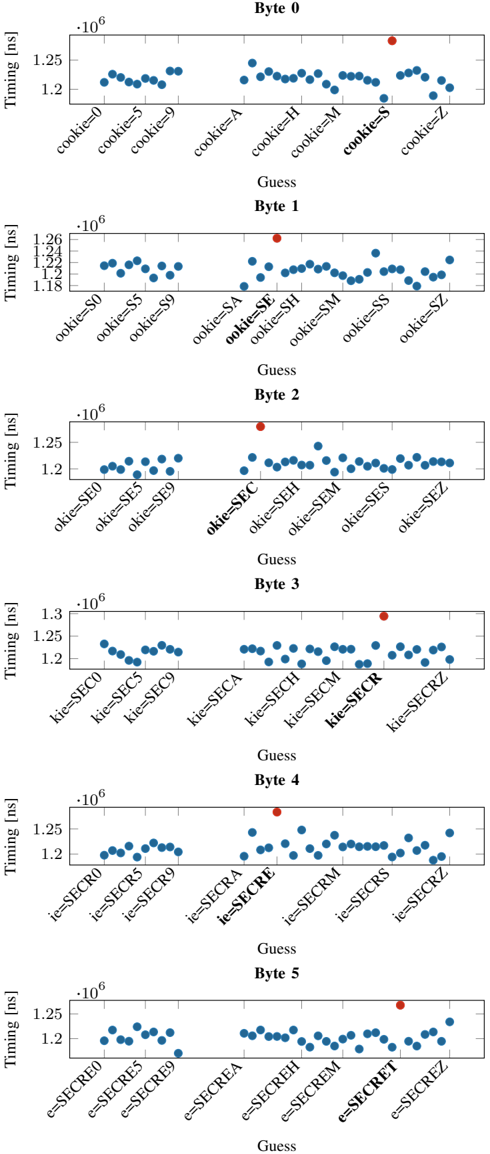<details> <summary>Image 20 Details</summary>  ### Visual Description \n ## Scatter Plot: Timing vs. Guess for Cookie Bytes ### Overview The image presents six scatter plots arranged vertically. Each plot represents a different byte (Byte 0 through Byte 5) of a "cookie" and shows the relationship between a "Guess" value and the corresponding "Timing" in nanoseconds (ns). Each plot displays timing data for various guesses, represented by different labels along the x-axis. A red data point is present in each plot, seemingly marking a specific guess. ### Components/Axes * **X-axis:** "Guess" - Categorical variable representing different cookie byte guesses. The labels vary for each byte, including "cookie=0", "cookie=5", "cookie=9", "cookie=A", "cookie=H", "cookie=M", "cookie=S", "cookie=Z" for Byte 0, and similar variations for Bytes 1-5. * **Y-axis:** "Timing [ns]" - Numerical variable representing the time taken in nanoseconds. The scale ranges from approximately 1.1 x 10⁶ to 1.3 x 10⁶ ns, with varying ranges for each byte. * **Data Points:** Blue scatter points representing the timing for each guess. A single red scatter point is present in each plot. * **Title:** Each plot is labeled with "Byte X" (where X is 0-5). * **Grid:** A light gray grid is present in the background of each plot. ### Detailed Analysis or Content Details **Byte 0:** * Trend: The blue data points are relatively flat, showing minimal variation in timing across different guesses. * Data Points (approximate): * cookie=0: 1.23 x 10⁶ ns * cookie=5: 1.24 x 10⁶ ns * cookie=9: 1.24 x 10⁶ ns * cookie=A: 1.23 x 10⁶ ns * cookie=H: 1.24 x 10⁶ ns * cookie=M: 1.23 x 10⁶ ns * cookie=S: 1.24 x 10⁶ ns * cookie=Z: 1.23 x 10⁶ ns * Red Point: cookie=S, 1.25 x 10⁶ ns **Byte 1:** * Trend: The blue data points show a slight upward trend as the guess value increases. * Data Points (approximate): * ookie=S0: 1.14 x 10⁶ ns * ookie=S5: 1.16 x 10⁶ ns * ookie=S9: 1.18 x 10⁶ ns * ookie=SA: 1.19 x 10⁶ ns * ookie=SE: 1.20 x 10⁶ ns * ookie=SH: 1.21 x 10⁶ ns * ookie=SM: 1.22 x 10⁶ ns * ookie=SS: 1.23 x 10⁶ ns * ookie=SZ: 1.24 x 10⁶ ns * Red Point: ookie=SZ, 1.25 x 10⁶ ns **Byte 2:** * Trend: Similar to Byte 1, a slight upward trend is observed. * Data Points (approximate): * okie=SE0: 1.20 x 10⁶ ns * okie=SE5: 1.21 x 10⁶ ns * okie=SE9: 1.22 x 10⁶ ns * okie=SEC: 1.23 x 10⁶ ns * okie=SEH: 1.24 x 10⁶ ns * okie=SEM: 1.25 x 10⁶ ns * okie=SES: 1.24 x 10⁶ ns * okie=SEZ: 1.25 x 10⁶ ns * Red Point: okie=SEZ, 1.26 x 10⁶ ns **Byte 3:** * Trend: A more pronounced upward trend is visible. * Data Points (approximate): * kie=SEC0: 1.18 x 10⁶ ns * kie=SEC5: 1.20 x 10⁶ ns * kie=SEC9: 1.22 x 10⁶ ns * kie=SECA: 1.23 x 10⁶ ns * kie=SECH: 1.24 x 10⁶ ns * kie=SECM: 1.25 x 10⁶ ns * kie=SECR: 1.24 x 10⁶ ns * kie=SECRZ: 1.26 x 10⁶ ns * Red Point: kie=SECRZ, 1.27 x 10⁶ ns **Byte 4:** * Trend: A clear upward trend is observed. * Data Points (approximate): * ie=SECRO: 1.20 x 10⁶ ns * ie=SECRS: 1.21 x 10⁶ ns * ie=SECRO9: 1.22 x 10⁶ ns * ie=SECREA: 1.23 x 10⁶ ns * ie=SECREH: 1.24 x 10⁶ ns * ie=SECREM: 1.25 x 10⁶ ns * ie=SECRR: 1.24 x 10⁶ ns * ie=SECRZ: 1.26 x 10⁶ ns * Red Point: ie=SECRZ, 1.27 x 10⁶ ns **Byte 5:** * Trend: A clear upward trend is observed. * Data Points (approximate): * e=SECRET0: 1.20 x 10⁶ ns * e=SECRET5: 1.21 x 10⁶ ns * e=SECRET9: 1.22 x 10⁶ ns * e=SECRETA: 1.23 x 10⁶ ns * e=SECRETH: 1.24 x 10⁶ ns * e=SECRETM: 1.25 x 10⁶ ns * e=SECRETR: 1.24 x 10⁶ ns * e=SECREZ: 1.26 x 10⁶ ns * Red Point: e=SECREZ, 1.27 x 10⁶ ns ### Key Observations * The red data point consistently appears at the highest "Guess" value for each byte. * The timing generally increases with increasing "Guess" values, particularly from Byte 1 onwards. * Byte 0 shows the least variation in timing. * The timing scales vary slightly between the bytes. ### Interpretation The plots likely represent a timing attack or side-channel analysis on a system that uses a cookie for authentication or security. The "Guess" values represent attempts to predict the cookie byte by byte. The "Timing" represents the time taken to perform a comparison or operation related to the cookie. The upward trend in timing as the "Guess" value increases suggests that the comparison process takes longer when the guess is closer to the correct value. This is a common characteristic of timing attacks, where attackers can infer information about the secret cookie by measuring the time it takes for the system to respond to different guesses. The red data point consistently appearing at the highest guess value and longest timing suggests that this guess is the correct one for that byte. The fact that Byte 0 shows minimal timing variation might indicate that this byte is either less sensitive or protected by a different mechanism. The data suggests a vulnerability to timing attacks, as the timing information leaks information about the cookie. Further analysis would be needed to determine the severity of the vulnerability and potential mitigation strategies. The consistent pattern across bytes indicates a systematic timing leak, rather than random noise. </details> Timing [ns] . cookie=SECR0 cookie=SECR5 Timing [ns] , , cookie=SECRE9 cookie=SECRE0 cookie=SECRE5 cookie=SECREA cookie=SECR9 cookie=SECRA Byte 4 cookie=SECRS cookie=SECRE cookie=SECRM Byte 5 cookie=SECREH cookie=SECREM Guess Fig. 17: Bytewise leakage of the last two bytes of the secret (E,T) from ZRAM. Times for guesses (0-9, A-Z) for each of the bytes are shown. The highest value in each plot (shown in red) indicates the correct secret value for the byte. . cookie=SECRZ cookie=SECREZ cookie=SECRET