2111.10882v1

# Geometry-Aware Multi-Task Learning for Binaural Audio Generation from Video **Authors**: Rishabh Garg, Ruohan Gao, Kristen Grauman ## Geometry-Aware Multi-Task Learning for Binaural Audio Generation from Video Rishabh Garg 1 rishabh@cs.utexas.edu Ruohan Gao 2 rhgao@cs.stanford.edu Kristen Grauman 1,3 grauman@cs.utexas.edu 1 The University of Texas at Austin 2 Stanford University 3 Facebook AI Research ## Abstract Binaural audio provides human listeners with an immersive spatial sound experience, but most existing videos lack binaural audio recordings. We propose an audio spatialization method that draws on visual information in videos to convert their monaural (singlechannel) audio to binaural audio. Whereas existing approaches leverage visual features extracted directly from video frames, our approach explicitly disentangles the geometric cues present in the visual stream to guide the learning process. In particular, we develop a multi-task framework that learns geometry-aware features for binaural audio generation by accounting for the underlying room impulse response, the visual stream's coherence with the sound source(s) positions, and the consistency in geometry of the sounding objects over time. Furthermore, we introduce a new large video dataset with realistic binaural audio simulated for real-world scanned environments. On two datasets, we demonstrate the efficacy of our method, which achieves state-of-the-art results. ## Introduction Both sight and sound are key drivers of the human perceptual experience, and both convey essential spatial information. For example, a car driving past us is audible-and spatially trackable-even before it crosses our field of view; a bird singing high in the trees helps us spot it with binoculars; a chamber music quartet performance sounds spatially rich, with the instruments' layout on stage affecting our listening experience. Spatial hearing is possible thanks to the binaural audio received by our two ears. The Interaural Level Difference (ILD) and the Interaural Time Difference (ITD) between the sounds reaching each ear, as well as the shape of the outer ears themselves, all provide spatial effects [42]. Meanwhile, the reflections and reverberations of sound in the environment are a function of the room acoustics-the geometry of the room, its major surfaces, and their materials. For example, we perceive the same audio differently in a long corridor versus a large room, or a room with heavy carpet versus a smooth marble floor. Videos or other media with binaural audio imitate that rich audio experience for a user, making the media feel more real and immersive. This immersion is important for virtual ©2021. The copyright of this document resides with its authors. 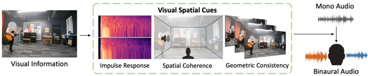Figure 1: To generate accurate binaural audio from monaural audio, the visuals provide significant cues that can be learnt jointly with audio prediction. Our approach learns to extract spatial information (e.g., the guitar player is on the left), geometric consistency of the position of the sound sources over time, and cues from the inferred binaural impulse response from the surrounding room. <details> <summary>Image 1 Details</summary>  ### Visual Description ## Diagram: Visual to Binaural Audio Conversion ### Overview The image illustrates a process of converting visual information into binaural audio, incorporating spatial cues. It starts with visual input, extracts spatial information, and transforms it into audio signals that simulate how sound is perceived by human ears. ### Components/Axes The diagram consists of the following components, arranged from left to right: 1. **Visual Information:** A photograph of a person playing a guitar in a room. * Label: "Visual Information" is located below the photograph. 2. **Impulse Response:** Two spectrogram-like plots, one above the other, showing frequency content over time. The plots are primarily colored in shades of orange, red, and purple. * Label: "Impulse Response" is located below the plots. 3. **Spatial Coherence:** A 3D wireframe representation of a room, with a speaker icon on the left wall and a silhouette of a person in the center. The background shows a blurred image of the room. * Label: "Spatial Coherence" is located below the wireframe. 4. **Geometric Consistency:** A series of overlapping images of the same scene, suggesting different viewpoints or perspectives. * Label: "Geometric Consistency" is located below the images. 5. **Mono Audio:** A waveform representation of a single-channel audio signal. * Label: "Mono Audio" is located above the waveform. 6. **Binaural Audio:** A silhouette of a head with two waveforms emanating from the ears. The waveform on the left is orange, and the waveform on the right is blue. * Label: "Binaural Audio" is located below the silhouette. A dashed green border encloses the "Impulse Response," "Spatial Coherence," and "Geometric Consistency" components, with the label "Visual Spatial Cues" at the top. ### Detailed Analysis * **Visual Information:** The initial input is a visual scene, providing the basis for spatial understanding. * **Impulse Response:** The spectrograms likely represent the acoustic characteristics of the room, showing how sound reflects and reverberates. The colors indicate the intensity of different frequencies over time. * **Spatial Coherence:** The wireframe model and speaker icon represent the spatial layout of the room and the position of the sound source. The silhouette indicates the listener's position. * **Geometric Consistency:** The overlapping images suggest that the system considers multiple viewpoints to ensure accurate spatial representation. * **Mono Audio:** A single-channel audio signal is processed to create a binaural experience. * **Binaural Audio:** The final output is a two-channel audio signal designed to simulate how sound is perceived by the left and right ears, creating a sense of spatial audio. ### Key Observations * The diagram illustrates a pipeline that transforms visual information into binaural audio. * Spatial cues are extracted from the visual scene and used to create a realistic audio experience. * The process involves analyzing the acoustic properties of the environment, modeling the spatial layout, and considering multiple viewpoints. ### Interpretation The diagram demonstrates a method for creating spatial audio from visual input. By analyzing the visual scene, the system can extract spatial cues that are used to generate binaural audio, providing a more immersive and realistic listening experience. This technology could be used in applications such as virtual reality, gaming, and teleconferencing to enhance the sense of presence and spatial awareness. The use of impulse response, spatial coherence, and geometric consistency suggests a sophisticated approach to capturing and reproducing spatial audio information. </details> reality and augmented reality applications, where the user should feel transported to another place and perceive it as such. However, collecting binaural audio data is a challenge. Presently, spatial audio is collected with an array of microphones or specialized dummy rig that imitates the human ears and head. The collection process is therefore less accessible and more costly compared to standard single-channel monaural audio captured with ease from today's ubiquitous mobile devices. Recent work explores how monaural audio can be upgraded to binaural audio by leveraging the visual stream in videos [23, 34, 63]. The premise is that the visual context provides hints for how to spatialize the sound due to the visible sounding objects and room geometry. While inspiring, existing models are nonetheless limited to extracting generic visual cues that only implicitly infer spatial characteristics. Our idea is to explicitly model the spatial phenomena in video that influence the associated binaural sound. Going beyond generic visual features, our approach guides binauralization with those geometric cues from the object and environment that dictate how a listener receives the sound in the real world. In particular, we introduce a multi-task learning framework that accounts for three key factors (Fig. 1). First, we require the visual features to be predictive of the room impulse response (RIR), which is the transfer function between the sound sources, 3D environment, and camera/microphone position. Second, we require the visual features to be spatially coherent with the sound, i.e., they can understand the difference when audio is aligned with the visuals and when it is not. Third, we enforce the geometric consistency of objects over time in the video. Whereas existing methods treat audio and visual frame pairs as independent samples, our approach represents the spatio-temporal smoothness of objects in video, which generally do not have dramatic instantaneous changes in their layout. The main contributions of this work are as follows. Firstly, we propose a novel multitask approach to convert a video's monaural sound to binaural sound by learning audio-visual representations that leverage geometric characteristics of the environment and the spatial and temporal cues from videos. Second, to facilitate binauralization research, we create SimBinaural, a large-scale dataset of simulated videos with binaural sound in photo-realistic 3D indoor scene environments. This new dataset facilitates both learning and quantitative evaluation, allows us to explore the impact of particular parameters in a controlled manner, and even benefits learning in real videos. Finally, we show the efficacy of our method via extensive experiments in generating realistic binaural audio, achieving state-of-the-art results. ## 2 Related Work Visually-Guided Audio Spatialization Recent work uses video frames to provide a form of self-supervision to implicitly infer the relative positions of sound-making objects. They formulate the problem as an upmixing task from mono to binaural using the visual information. Morgado et al . [34] use 360 videos from YouTube to predict first order ambisonic sound useful for 360 viewing, while Lu et al . [32] use a self-supervised audio spatialization network using visual frames and optical flow. Whereas [32] uses correspondence to learn audio synthesizer ratio masks, which does not necessitate understanding of sound making objects, we enforce understanding of the sound location via spatial coherence in the visual features. For speech synthesis, using the ground truth position and orientation of the source and receiver instead of a video is also explored [43]. More closely related to our problem, the 2.5D visual sound approach by Gao and Grauman generates binaural audio from video [23]. Building on those ideas, Zhou et al . [63] propose an associative pyramid network (APNet) architecture to fuse the modalities and jointly train on audio spatialization and source separation task. Concurrent to our work, Xu et al . [57] propose to generate binaural audio for training from mono audio by using spherical harmonics. In contrast to these methods, we explore a novel framework for learning geometric representations, and we introduce a large-scale photo-realistic video dataset with acoustically accurate binaural information (which will be shared publicly). We outperform the existing methods and show that the new dataset can be used to augment performance. Audio and 3D Spaces Recent work exploits the complementary nature of audio and the characteristics of the environment in which it is heard or recorded. Prior methods estimate the acoustic properties of materials [47], estimate reverberation time and equalization of the room using an actual 3D model of a room [50], and learn audio-visual correspondence from video [58]. Chen et al . [7] introduce the SoundSpaces audio platform to perform audio-visual navigation in scanned 3D environments, using binaural audio to guide policy learning. Ongoing work continues to explore audio-visual navigation models for embodied agents [8, 9, 14, 21, 33]. Other work predicts depth maps using spatial audio [11] and learns representations via interaction using echoes recorded in indoor 3D simulated environments [25]. In contrast to all of the above, we are interested in a different problem of generating accurate spatial binaural sound from videos. We do not use it for navigation nor to explicitly estimate information about the environment. Rather, the output of our model is spatial sound to provide a human listener with an immersive audio-visual experience. Audio-Visual Learning Audio-visual learning has a long history, and has enjoyed a resurgence in the vision community in recent years. Cross-modal learning is explored to understand the natural synchronisation between visuals and the audio [3, 5, 39]. Audio-visual data is leveraged for audio-visual speech recognition [12, 28, 59, 62], audio-visual event localization [51, 52, 55], sound source localization [4, 29, 45, 49, 51, 60], self-supervised representation learning [25, 31, 35, 37, 39], generating sounds from video [10, 19, 38, 64], and audio-visual source separation for speech [1, 2, 13, 16, 18, 37], music [20, 22, 56, 60, 61], and objects [22, 24, 53]. In contrast to all these methods, we perform a different task: to produce binaural two-channel audio from a monaural audio clip using a video's visual stream. ## 3 Approach Our goal is to generate binaural audio from videos with monaural audio. In this section, we first formally describe the problem (Section 3.1). 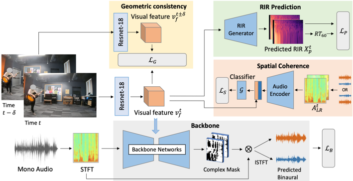Then we introduce our proposed multi-task Figure 2: Proposed network. The network takes the visual frames and monaural audio as input. The ResNet-18 visual features v t f are trained in a multi-task setting. The features v t f are used to directly predict the RIR via a decoder (top right). Audio features from binaural audio, which might have flipped channels, are combined with v t f and used to train a spatial coherence classifier G (middle right). Two temporally adjacent frames are also used to ensure geometric consistency (top center). The features v t f are jointly trained with the backbone network (bottom) to predict the final binaural audio output. <details> <summary>Image 2 Details</summary>  ### Visual Description ## Neural Network Architecture Diagram: Binaural Audio Prediction ### Overview The image presents a diagram of a neural network architecture designed for binaural audio prediction. The architecture incorporates visual and audio inputs, processes them through several modules including ResNet-18, RIR prediction, and spatial coherence analysis, and ultimately predicts binaural audio output. The diagram illustrates the flow of data and the interactions between different components of the network. ### Components/Axes * **Input:** * Two images: "Time t - δ" and "Time t" * Mono Audio * **Modules:** * ResNet-18 (used twice) * Backbone Networks * RIR Generator * Classifier * Audio Encoder * **Outputs:** * Predicted Binaural Audio * **Loss Functions:** * L_G (Geometric consistency) * L_P (RIR Prediction) * L_S (Spatial Coherence) * L_B (Binaural Prediction) * **Intermediate Representations:** * Visual feature v_f^t±δ * Visual feature v_f^t * STFT (Short-Time Fourier Transform) of Mono Audio * Predicted RIR X_p^t * A^t_LR * Complex Mask ### Detailed Analysis 1. **Input Branch (Visual):** * Two images, captured at "Time t - δ" and "Time t", are fed into ResNet-18 networks. * The ResNet-18 networks extract visual features v_f^t±δ and v_f^t. * The visual features are used for geometric consistency, resulting in a loss L_G. 2. **Input Branch (Audio):** * Mono audio is transformed into its Short-Time Fourier Transform (STFT) representation. * The STFT representation is fed into "Backbone Networks". * The output of the "Backbone Networks" is a "Complex Mask". 3. **RIR Prediction Branch:** * The visual feature v_f^t±δ is fed into an "RIR Generator". * The RIR Generator predicts the Room Impulse Response (RIR) X_p^t. * The predicted RIR is associated with a reverberation time RT₆₀. * The RIR prediction is associated with a loss L_P. 4. **Spatial Coherence Branch:** * The visual feature v_f^t is fed into a "Classifier". * The output of the classifier is combined with the output of an "Audio Encoder". * The output of the Audio Encoder is A^t_LR. * The spatial coherence is associated with a loss L_S. 5. **Backbone and Binaural Prediction:** * The Complex Mask from the audio branch is combined (multiplied) with the output of the spatial coherence branch (A^t_LR). * The result is processed by an Inverse Short-Time Fourier Transform (ISTFT) to produce the "Predicted Binaural" audio. * The binaural prediction is associated with a loss L_B. ### Key Observations * The architecture integrates visual and audio information to predict binaural audio. * ResNet-18 is used to extract visual features from images at different time points. * The RIR prediction branch aims to model the acoustic characteristics of the environment. * The spatial coherence branch aims to capture the spatial relationships between audio sources. * Loss functions are used to train the different modules of the network. ### Interpretation The diagram illustrates a sophisticated approach to binaural audio prediction by leveraging both visual and audio cues. The use of ResNet-18 for visual feature extraction, combined with RIR prediction and spatial coherence analysis, suggests that the network attempts to model the acoustic environment and the spatial relationships between audio sources. The integration of these components allows the network to generate a more realistic and immersive binaural audio experience. The different loss functions (L_G, L_P, L_S, L_B) indicate that the network is trained to optimize geometric consistency, RIR prediction accuracy, spatial coherence, and binaural audio quality. The architecture is designed to learn the complex relationships between visual scenes and the corresponding binaural audio, enabling it to predict how sound would be perceived in a given environment. </details> setting (Section 3.2). Next we describe the training and inference method (Section 3.3), and finally we describe the proposed SimBinaural dataset (Section 3.4). ## 3.1 Problem Formulation Our objective is to map the monaural sound from a given video to spatial binaural audio. The input video may have one or more sound sources, and neither their positions in the 3D scene nor their positions in the 2D video frame are given. For a video V with frames { v 1 ... v T } and monaural audio a t M , we aim to predict a two channel binaural audio output { a t L , a t R } . Whereas a single-channel audio a t M lacks spatial characteristics, two-channel binaural audio { a t L , a t R } conveys two distinct waveforms to the left and right ears separately and hence provides spatial effects to the listener. By coupling the monaural audio with the visual stream, we aim to leverage the spatial cues from the pixels to infer how to spatialize the sound. We first transfer the input audio waveforms into the time-frequency domain using the Short-Time Fourier Transformation (STFT). We aim to predict the binaural audio spectrograms {A t L , A t R } from the input mono spectrogram A t M , where A t X = STFT ( a t X ) , conditioned on visual features v t f from the video frames at time t . ## 3.2 Geometry-Aware Multi-Task Binauralization Network Our approach has four main components: the backbone for converting mono audio to binaural by injecting the visual information, the spatial coherence module that learns the relative alignment of the spatial sound and frame, an RIR prediction module that requires the room impulse response to be predictable from the video frames, and the geometric consistency module that enforces consistency of objects over time. Backbone Loss First, we define the backbone loss within our multi-task framework (Fig. 2, bottom). This backbone network is used to transform the input monaural spectrogram A t M to binaural ones. During training, the mono audio is obtained by averaging the two channels a t M =( a t L + a t R ) / 2 and hence the spatial information is lost. Rather than directly predict the two channels of binaural output, we predict the difference of the two channels, following [23]. This better captures the subtle distinction of the channels and avoids collapse to the easy case of predicting the same output for both channels. We predict a complex mask M t D , which, multiplied with the original audio spectrogram A t M , gives the predicted difference spectrogram A t D ( pred ) = M t D · A t M . The true difference spectrogram of the training input A t D is the STFT of a t L -a t R . We minimize the distance between these two spectrograms: ‖A t D -A t D ( pred ) ‖ 2 2 . We also predict the two channels via two complex masks M t L and M t R , one for each channel, to obtain the predicted channel spectrograms A t L ( pred ) and A t R ( pred ) like above. This gives us the overall backbone objective: <!-- formula-not-decoded --> Spatial Coherence We encourage the visual features to have geometric understanding of the relative positions of the sound source and receiver via an audio-visual feature alignment prediction term. This loss requires the predicted audio to correctly capture which channel is left and right with respect to the visual information. This is crucial to achieve the proper spatial effect while watching videos, as the audio needs to match the observed visuals' layout. In particular, we incorporate a classifier to identify whether the visual input is aligned with the audio. The classifier G combines the binaural audio A LR = {A t L , A t R } and the visual features v t f to classify if the audio and visuals agree. In this way, the visual features are forced to reason about the relative positions of the sound sources and learn to find the cues in the visual frames which dictate the direction of sound heard. During training, the original ground truth samples are aligned, and we create misaligned samples by flipping the two channels in the ground truth audio to get A LR = {A t R , A t L } . We calculate the binary cross entropy (BCE) loss for the classifier's prediction of whether the audio is flipped or not, c = G ( A LR , v t f ) , and the indicator ˆ c denoting if the audio is flipped, yielding the spatial coherence loss: <!-- formula-not-decoded --> Room Impulse Response and Reverberation Time Prediction The third component of our multi-task model trains the visual features to be predictive of the room impulse response (RIR). An impulse response gives a concise acoustic description of the environment, consisting of the initial direct sound, the early reflections from the surfaces of the room, and a reverberant tail from the subsequent higher order reflections between the source and receiver. The visual frames convey information like the layout of the room and the sound source with respect to the receiver, which in part form the basis of the RIR. Since we want our audio-visual feature to be a latent representation of the geometry of the room and the source-receiver position pair, we introduce an auxiliary task to predict the room IR directly from the visual frames via a generator on the visual features. Furthermore, we require the features to be predictive of the reverberation time RT 60 metric, which is the time it takes the energy of the impulse to decay 60dB, and can be calculated from the energy decay curve of the IR [48]. The RT 60 is commonly used to characterize the sound properties of a room; we employ it as a low-dimensional target here to guide feature learning alongside the highdimensional RIR spectrogram prediction. We convert the ground truth binaural impulse response signal { rL , rR } to the frequency domain using the STFT and obtain magnitude spectrograms X for each channel. The IR prediction network consists of a generator which performs upconvolutions on the visual features v t f to obtain a predicted magnitude spectrogram X t ( pred ) . We minimize the euclidean distance between the predicted RIR X t ( pred ) , and the ground truth X t gt . Additionally, we obtain the RIR waveform from the predicted spectrogram X t ( pred ) via the Griffin-Lim algorithm [26, 41] and compute the RT 60 ( pred ) . We minimize the L1 distance between the predicted RT 60 ( pred ) and the ground truth RT 60 ( gt ) . Thus, the overall RIR prediction loss is: <!-- formula-not-decoded --> Geometric Consistency Since the videos are continuous samples over time rather than individual frames, our fourth and final loss regularizes the visual features by requiring them to have spatio-temporal geometric consistency. The position of the source(s) of sound and the position of the camera-as well as the physical environment where the video is recordeddo not typically change instantaneously in videos. Therefore, there is a natural coherence between the sound in a video observed at two points that are temporally close. Since visual features are used to condition our binaural prediction, we encourage our visual features to learn a latent representation that is coherent across short intervals of time. Specifically, the visual features v t f and v t ± d f should be relatively similar to each other to produce audio with fairly similar spatial effects. Specifically, the geometric consistency loss is: <!-- formula-not-decoded --> where a is the margin allowed between two visual features. We select a random frame ± 1 second from t , so -1 ≤ d ≤ 1. This ensures that similar placements of the camera with respect to the audio source should be represented with similar features, while the margin allows room for dissimilarity for the changes due to time. Since the underlying visual features are regularized to be similar, the predicted audio conditioned on these visual features is also encouraged to be temporally consistent. ## 3.3 Training and Inference During training, the mono audio is obtained by taking the mean of the two channels of the ground truth audio a t m =( a t L + a t R ) / 2. The visual features v t f are reduced in dimension, tiled, and concatenated with the output of the audio encoder to fuse the information from the audio and visual streams. The overall multi-task loss is a combination of the losses (Equations 1-4) described earlier: <!-- formula-not-decoded --> where l B , l S , l G and l P are the scalar weights used to determine the effect of each loss during training, set using validation data. To generate audio at test time, we only require the mono audio and visual frames. The predicted spectrograms are used to obtain the predicted difference signal a t D ( pred ) and two-channel audio { a t L , a t R } via an inverse Short-Time Fourier Transformation (ISTFT) operation. ## 3.4 SimBinaural Dataset Weexperiment with both real world video (FAIR-Play [23]) and video from scanned environments with high quality simulated audio. 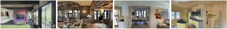For the latter, to facilitate large-scale experimentationand to augment learning from real videos-we create a new dataset called SimBinaural of Figure 3: Example frames from the SimBinaural dataset. <details> <summary>Image 3 Details</summary>  ### Visual Description ## Interior Design Collage ### Overview The image is a collage of four interior design photographs, each showcasing a different room or space within a home. The styles range from modern to rustic, with varying color palettes and architectural features. ### Components/Axes * **Image 1:** A modern living room with a purple accent wall, a large flat-screen TV, and contemporary furniture. * **Image 2:** A sunroom or hallway with large windows offering an outdoor view. * **Image 3:** A rustic living room with wood paneling, exposed beams, and traditional furniture. A guitar is visible in the background. * **Image 4:** A transitional space with a view into a dining room or office. Artwork and decorative items are visible. * **Image 5:** A kitchen with light wood paneling, a window, and modern appliances. A trumpet graphic is superimposed on the image. ### Detailed Analysis or ### Content Details * **Image 1:** The living room features a light-colored sofa, a dark ceiling with exposed beams, and a purple accent wall. A flat-screen TV is mounted on the purple wall. Artwork is visible on the adjacent white wall. * **Image 2:** The sunroom/hallway has a series of large windows with dark frames. The view outside is of greenery. The floor is a dark color. * **Image 3:** The rustic living room has wood paneling on the walls and exposed beams on the ceiling. A large arched doorway leads to another room. Traditional furniture, including a sofa and chairs, is present. A guitar is visible in the background. * **Image 4:** This transitional space features light-colored walls and a view into a dining room or office. Artwork and decorative items are visible on the walls. * **Image 5:** The kitchen has light wood paneling on the walls and ceiling. A window provides natural light. Modern appliances are visible, including a stove and refrigerator. A trumpet graphic is superimposed on the image. ### Key Observations * The collage presents a variety of interior design styles, from modern to rustic. * Each image showcases different architectural features and color palettes. * The presence of artwork, furniture, and decorative items adds character to each space. * The trumpet graphic in the kitchen image is an anomaly and does not appear to be part of the original design. ### Interpretation The collage appears to be a collection of interior design ideas or inspiration. The variety of styles suggests a broad range of tastes and preferences. The images could be used to showcase different design possibilities or to inspire homeowners to create their own unique spaces. The trumpet graphic in the kitchen image is likely a decorative element added for visual interest or to represent a specific theme. </details> Table 1: A comparison of the data in FAIR-Play and the large scale data we generated. | Dataset | #Videos | Length (hrs) | #Rooms | RIR | |----------------|-----------|----------------|----------|-------| | FAIR-Play [23] | 1,871 | 5.2 | 1 | No | | SimBinaural | 21,737 | 116.1 | 1,020 | Yes | simulated videos in photo-realistic 3D indoor scene environments. 1 The generated videos, totalling over 100 hours, resemble real-world audio recordings and are sampled from 1,020 rooms in 80 distinct environments; each environment is a multi-room home. Using the publicly available SoundSpaces 2 audio simulations [7] together with the Habitat simulator [46], we create realistic videos with binaural sounds for publicly available 3D environments in Matterport3D [6]. See Fig. 3 and Supp. video. Our resulting dataset is much larger and more diverse than the widely used FAIR-Play dataset [23] which is real video but is limited to 5 hours of recordings in one room (Table 1). To construct the dataset, we insert diverse 3D models from poly.google.com of various instruments like guitar, violin, flute etc. and other sound-making objects like phones and clocks into the scene. To generate realistic binaural sound in the environment as if it is coming from the source location and heard at the camera position, we convolve the appropriate SoundSpaces [7] room impulse response with an anechoic audio waveform (e.g., a guitar playing for an inserted guitar 3D object). Using this setup, we capture videos with simulated binaural sound. The virtual camera and attached microphones are moved along trajectories such that the object remains in view, leading to diversity in views of the object and locations within each video clip. Please see Supp. for details. ## 4 Experiments We validate our approach on both FAIR-Play [23] (an existing real video benchmark) and our new SimBinaural dataset. We compare to the following baselines: - Flipped-Visual: We flip the visual frame horizontally to provide incorrect visual information while testing. The other settings are the same as our method. - Audio Only: We provide only monaural audio as input, with no visual frames, to verify if the visual information is essential to learning. - Mono-Mono: Both channels have the same input monaural audio repeated as the twochannel output to verify if we are actually distinguishing between the channels. - Mono2Binaural [23] : A state-of-the-art 2.5D visual sound model for this task. We use the authors' code to evaluate in the settings as ours. - APNet [63] : A state-of-the-art model that handles both binauralization and audio source separation. We use the APNet network from their method and train only on binaural data (rather than stereo audio). We use the authors' code. 1 The SimBinaural dataset was constructed at, and will be released by, The University of Texas at Austin. 2 SoundSpaces [7] provides room impulse responses at a spatial resolution of 1 meter. These state-of-the-art RIRs capture how sound from each source propagates and interacts with the surrounding geometry and materials, modeling all of the major real-world features of the RIR: direct sounds, early specular/diffuse reflections, reverberations, binaural spatialization, and frequency dependent effects from materials and air absorption. Table 2: Binaural audio prediction errors on the FAIR-Play and SimBinaural datasets. For both metrics, lower is better. | | FAIR-Play | FAIR-Play | SimBinaural | SimBinaural | SimBinaural | SimBinaural | |--------------------|-------------|-------------|---------------|---------------|----------------|----------------| | | | | Scene-Split | Scene-Split | Position-Split | Position-Split | | | STFT | ENV | STFT | ENV | STFT | ENV | | Mono-Mono | 1.215 | 0.157 | 1.356 | 0.163 | 1.348 | 0.168 | | Audio-Only | 1.102 | 0.145 | 0.973 | 0.135 | 0.932 | 0.130 | | Flipped-Visual | 1.134 | 0.152 | 1.082 | 0.142 | 1.075 | 0.141 | | Mono2Binaural [23] | 0.927 | 0.142 | 0.874 | 0.129 | 0.805 | 0.124 | | APNet [63] | 0.904 | 0.138 | 0.857 | 0.127 | 0.773 | 0.122 | | Backbone+IR Pred | n/a | n/a | 0.801 | 0.124 | 0.713 | 0.117 | | Backbone+Spatial | 0.873 | 0.134 | 0.837 | 0.126 | 0.756 | 0.120 | | Backbone+Geom | 0.874 | 0.135 | 0.828 | 0.125 | 0.731 | 0.118 | | Our Full Model | 0.869 | 0.134 | 0.795 | 0.123 | 0.691 | 0.116 | - PseudoBinaural [57] : A state-of-the-art model that uses additional data to augment training. We use the authors' public pre-trained model. We evaluate two standard metrics, following [23, 34, 63]: 1) STFT Distance , the euclidean distance between the predicted and ground truth STFT spectrograms, which directly measures how accurate is our produced spectrogram, 2) Envelope Distance (ENV) which measures the euclidean distance between the envelopes of the predicted raw audio signal and the ground truth and can further capture the perceptual similarity. Implementation details All networks are written in PyTorch [40]. The backbone network is based upon the networks used for 2.5D visual sound [23] and APNet [63]. The audio network consists of a U-Net [44] type architecture while the RIR generator is adapted from GANSynth [15]. To preprocess both datasets, we follow the standard steps from [23]. We resample all the audio to 16kHz and for training the backbone, we use 0.63s clips of the 10s audio and the corresponding frame. Frames are extracted at 10fps. The visual frames are randomly cropped to 448 × 224. For testing, we use a sliding window of 0.1s to compute the binaural audio for all methods. Please see Supp. for more details. SimBinaural results We evaluate on two data splits: 1) Scene-Split , where the train and test set have disjoint scenes from Matterport3D [6] and hence the room of the videos at test time has not been seen before; and 2) Position-Split , where the splits may share the same Matterport3D scene/room but the exact configuration of the source object and receiver position is not seen before. Table 2 (right) shows the results. The table also ablates the parts of our model. Our model outperforms all the baselines, including the two state-of-the-art prior methods. In addition, Table 2 confirms that Scene-Split is a fundamentally harder task. This is because we must predict the sound, as well as other characteristics like the IR, from visuals distinct from those we have observed before. This forces the model to generalize its encoding to generic visual properties (wall orientations, major furniture, etc.) that have intra-class variations and geometry changes compared to the training scenes. The ablations shed light on the impact of each of the proposed losses in our multi-task framework. The full model uses all the losses as in Eqn 5. This outperforms other methods significantly on both splits. It also outperforms using each of the losses individually, which demonstrates the losses can combine to jointly learn better visual features for generating spatial audio. FAIR-Play results Table 2 (left) shows the results on the real video benchmark FAIR-Play using the standard split. Here, we omit the IR prediction network for our method, since FAIR-Play lacks ground truth impulse responses (which we need for training). The Backbone+Spatial and Backbone+Geom are the same as above. Both Table 3: Results on FAIR-Play when additional data is used for training. | Method | STFT | ENV | |---------------------|--------|-------| | APNet [63] | 1.291 | 0.162 | | PseudoBinaural [57] | 1.268 | 0.161 | | Ours | 1.234 | 0.16 | | Ours+SimBinaural | 1.175 | 0.154 | variants of our method outperform the state-of-the-art. Therefore, enforcing the geometric and spatial constraints is beneficial to the binaural audio generation task. We get the best results when we combine both the losses in our framework. To further evaluate the utility of our SimBinaural dataset, we next jointly train with both SimBinaural and FAIR-Play, then test on a challenging split of FAIR-Play in which the test scenes are non overlapping, as proposed in [57]. We compare our method with AugmentPseudoBinaural [57] 3 which also uses additional generated training data. Our method with SimBinaural outperforms other methods (Table 3). This is an important result, as it demonstrates that SimBinaural can be leveraged to improve performance on real video. 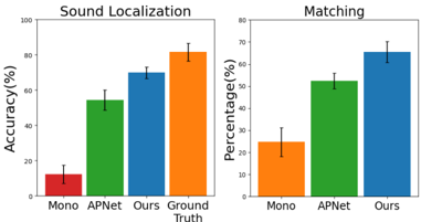User study Next, we present two user studies to validate whether the predicted binaural sound does indeed provide an immersive and spatially accurate experience for human listeners. Twenty participants with normal hearing were presented with 20 videos from the test set of the two datasets. They were asked to rate the quality in two ways: 1) users were given only the audio and asked to choose from which di- <details> <summary>Image 4 Details</summary>  ### Visual Description ## Bar Chart: Sound Localization and Matching Accuracy ### Overview The image presents two bar charts comparing the performance of different methods (Mono, APNet, Ours) against Ground Truth in Sound Localization and Matching tasks. The charts display accuracy and percentage metrics, respectively, with error bars indicating variability. ### Components/Axes **Left Chart (Sound Localization):** * **Title:** Sound Localization * **Y-axis:** Accuracy (%) * Scale: 0 to 100 * **X-axis:** Methods (Mono, APNet, Ours, Ground Truth) * **Bars:** * Mono (Red) * APNet (Green) * Ours (Blue) * Ground Truth (Orange) **Right Chart (Matching):** * **Title:** Matching * **Y-axis:** Percentage (%) * Scale: 0 to 80 * **X-axis:** Methods (Mono, APNet, Ours) * **Bars:** * Mono (Orange) * APNet (Green) * Ours (Blue) ### Detailed Analysis **Left Chart (Sound Localization):** * **Mono (Red):** Accuracy is approximately 13% with an error bar extending from roughly 10% to 16%. * **APNet (Green):** Accuracy is approximately 55% with an error bar extending from roughly 50% to 60%. * **Ours (Blue):** Accuracy is approximately 70% with an error bar extending from roughly 67% to 73%. * **Ground Truth (Orange):** Accuracy is approximately 82% with an error bar extending from roughly 79% to 85%. **Right Chart (Matching):** * **Mono (Orange):** Percentage is approximately 25% with an error bar extending from roughly 20% to 30%. * **APNet (Green):** Percentage is approximately 52% with an error bar extending from roughly 49% to 55%. * **Ours (Blue):** Percentage is approximately 65% with an error bar extending from roughly 62% to 68%. ### Key Observations * In Sound Localization, Ground Truth achieves the highest accuracy, followed by "Ours," APNet, and Mono. * In Matching, "Ours" achieves the highest percentage, followed by APNet and Mono. * The "Ours" method consistently outperforms Mono and APNet in both tasks. * Error bars suggest some variability in the results, but the overall trends are clear. ### Interpretation The data suggests that the "Ours" method is a significant improvement over Mono and APNet for both Sound Localization and Matching tasks. While "Ours" does not reach the performance of Ground Truth in Sound Localization, it demonstrates a substantial increase in accuracy compared to the other methods. The error bars indicate that the observed differences are likely statistically significant. The charts highlight the effectiveness of the "Ours" method in these specific tasks. </details> Truth Figure 4: User study results. See text for details. rection (left/right/center) they heard the audio; 2) given a pair of audios and a reference frame, the users were asked to choose which audio gives a binaural experience closer to the provided ground truth. As can be seen in Fig. 4, users preferred our method both for the accuracy of the direction of sound (left) and binaural audio quality (right). 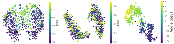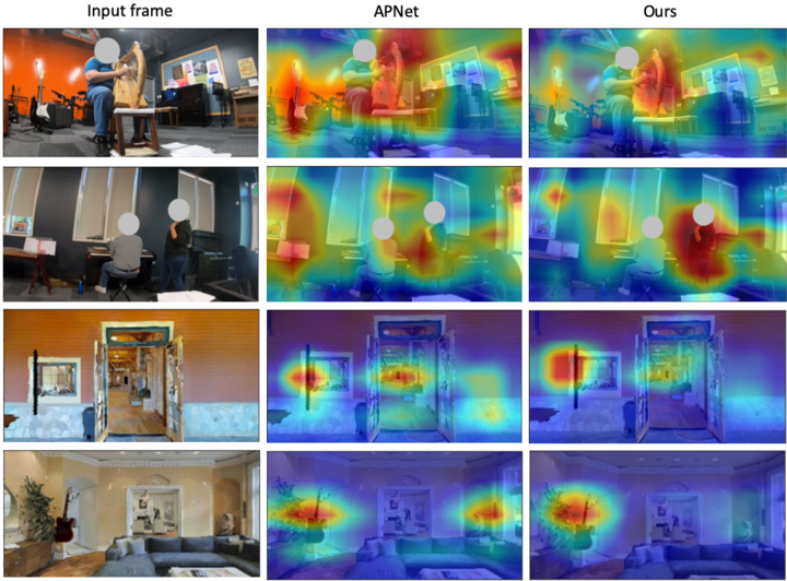Visualization Figure 5 shows the t-SNE projections [54] of the visual features from SimBinaural colored by the RT 60 of the audio clip. While the features from our method (left) can infer the RT 60 characteristics, the ones from APNet [63] (center) are randomly distributed. Simultaneously, our features also accurately capture the angle of the object from the center (right). Fig. 6 shows the activation maps of the visual network. While APNet produces more diffuse maps, our method localizes the object better within the image. This indicates that the visual features in our method are better at identifying the regions which might be emitting sound to generate more accurate binaural audio. ## 5 Conclusion We presented a multi-task approach to learn geometry-aware visual features for mono to binaural audio conversion in videos. Our method exploits the inherent room and object 3 The pre-trained model provided by PseudoBinaural [57] is trained on a different split instead of the standard split from [23] and hence it is not directly comparable in Table 2. We evaluate on the new split in Table 3. Figure 5: t-SNE of visual features colored by RT 60 for our method (left) and APNet (center); and colored by angle of the object from the center (right). <details> <summary>Image 5 Details</summary>  ### Visual Description ## Scatter Plots: RT60 and Angle Distributions ### Overview The image presents three scatter plots. The first two plots show the distribution of data points colored by RT60 values, while the third plot shows the distribution colored by Angle (degrees). Each plot displays a cluster of points, with color indicating the magnitude of the respective variable. ### Components/Axes * **Plot 1 & 2 Color Legend:** Located to the right of the first two plots. * **Label:** RT60 * **Scale:** Ranges from 0.2 (dark purple) to 1.0 (yellow). * **Plot 3 Color Legend:** Located to the right of the third plot. * **Label:** Angle (deg) * **Scale:** Ranges from -40 (dark purple) to 40 (yellow). ### Detailed Analysis **Plot 1: RT60 Distribution** * The data points form a roughly circular cluster. * Points with lower RT60 values (dark purple) are concentrated in the bottom and right regions of the cluster. * Points with higher RT60 values (yellow) are concentrated in the top and left regions of the cluster. * The RT60 values appear to transition smoothly across the cluster. **Plot 2: RT60 Distribution** * The data points are split into two distinct clusters. * In both clusters, points with lower RT60 values (dark purple) are located towards the bottom. * Points with higher RT60 values (yellow) are located towards the top. * There is a clear separation between the high and low RT60 value regions within each cluster. **Plot 3: Angle Distribution** * The data points are clustered in a non-uniform shape. * Points with negative angle values (dark purple) are concentrated in the bottom region. * Points with positive angle values (yellow) are concentrated in the top region. * The angle values transition from negative to positive in a roughly vertical direction. ### Key Observations * The RT60 values in the first plot show a gradient distribution, while in the second plot, they are clustered into distinct regions. * The angle values in the third plot show a clear separation between positive and negative values. * The color gradients in each plot provide a visual representation of the distribution of RT60 and angle values. ### Interpretation The plots visualize the distribution of RT60 and angle values across a dataset. The clustering and color gradients suggest potential relationships or patterns within the data. The first plot indicates a continuous variation of RT60, while the second plot suggests distinct groups with different RT60 characteristics. The third plot shows a clear separation between positive and negative angle values, which could indicate different states or conditions within the system being analyzed. Further analysis would be needed to understand the underlying factors driving these distributions and their significance. </details> Figure 6: Qualitative visualization of the activation maps for the visual network for APNet [63] and ours. We can see that while the activation maps for APNet [63] are diffused and focusing on nonessential parts like objects in the background, our method focuses more on the object/region producing the sound and its location. <details> <summary>Image 6 Details</summary>  ### Visual Description ## Image Comparison: Input Frame vs. APNet vs. Ours ### Overview The image presents a visual comparison of scene understanding between an "Input frame," "APNet," and "Ours." It consists of four rows, each depicting a different scene. The "Input frame" column shows the original image, while the "APNet" and "Ours" columns display heatmaps overlaid on the original images, presumably representing the focus or attention of each method. The heatmaps use a color gradient, with red indicating higher attention and blue indicating lower attention. The faces of people in the images are obscured with gray circles. ### Components/Axes * **Columns:** * Input frame * APNet * Ours * **Rows:** Each row represents a different scene. * Row 1: A person playing a harp in a room with musical instruments. * Row 2: Two people in a room with a piano and other equipment. * Row 3: An open doorway leading to another room. * Row 4: A living room with a couch, guitar, and other furniture. * **Heatmap Color Gradient:** Red indicates high attention, transitioning through yellow, green, and blue to indicate low attention. ### Detailed Analysis **Row 1: Harp Player** * **Input frame:** A person is seated and playing a harp. Guitars and other musical equipment are visible in the background. * **APNet:** The heatmap shows attention distributed across the person, the harp, and some background elements. The highest attention (red) is focused on the harp and the person's hands. * **Ours:** The heatmap is similar to APNet, with high attention (red) on the harp and the person's hands. The attention seems slightly more focused on the harp itself compared to APNet. **Row 2: Piano Scene** * **Input frame:** Two people are in a room. One person is seated at a piano, and another is standing nearby. * **APNet:** The heatmap shows attention focused on the person standing and the piano. The highest attention (red) is on the standing person. * **Ours:** The heatmap shows attention focused on the person standing and the piano. The highest attention (red) is on the standing person, similar to APNet. **Row 3: Doorway Scene** * **Input frame:** An open doorway leads to another room. A mirror is visible on the left wall. * **APNet:** The heatmap shows high attention (red) focused on the doorway and the mirror. * **Ours:** The heatmap shows high attention (red) focused on the doorway and the mirror, similar to APNet. **Row 4: Living Room Scene** * **Input frame:** A living room with a couch, a guitar leaning against the wall, and other furniture. * **APNet:** The heatmap shows high attention (red) focused on the guitar and the area around the doorway. * **Ours:** The heatmap shows high attention (red) focused on the guitar and the area around the doorway, similar to APNet. ### Key Observations * Both APNet and "Ours" methods generate heatmaps that highlight salient objects and regions in the scenes. * In most cases, the heatmaps generated by APNet and "Ours" are qualitatively similar, suggesting that both methods attend to similar features. * The heatmaps tend to focus on objects of interest, such as people, musical instruments, and doorways. ### Interpretation The image demonstrates a comparison of attention mechanisms between two methods, APNet and "Ours," in various scenes. The heatmaps suggest that both methods are capable of identifying and focusing on relevant objects and regions within the images. The similarity between the heatmaps generated by APNet and "Ours" indicates that both methods have a similar understanding of the scene's important elements. The heatmaps provide a visual representation of the model's focus, which can be useful for understanding how the model makes decisions and for identifying potential areas for improvement. </details> geometry and spatial information encoded in the visual frames to generate rich binaural audio. We also generated a large-scale video dataset with binaural audio in photo-realistic environments to better understand and learn the relation between visuals and binaural audio. This dataset will be made publicly available to support further research in this direction. Our state-of-the-art results on two datasets demonstrate the efficacy of our proposed formulation. In future work we plan to explore how semantic models of object categories' sounds could benefit the spatialization task. Acknowledgements Thanks to Changan Chen for help with experiments, Tushar Nagarajan for feedback on paper drafts, and the UT Austin vision group for helpful discussions. UT Austin is supported by NSF CNS 2119115 and a gift from Google. Ruohan Gao was supported by a Google PhD Fellowship. ## References - [1] Triantafyllos Afouras, Joon Son Chung, and Andrew Zisserman. The conversation: Deep audio-visual speech enhancement. In Interspeech , 2018. - [2] Triantafyllos Afouras, Joon Son Chung, and Andrew Zisserman. My lips are concealed: Audio-visual speech enhancement through obstructions. In ICASSP , 2019. - [3] Relja Arandjelovic and Andrew Zisserman. Look, listen and learn. In ICCV , 2017. - [4] Relja Arandjelovi´ c and Andrew Zisserman. Objects that sound. In ECCV , 2018. - [5] Yusuf Aytar, Carl Vondrick, and Antonio Torralba. Soundnet: Learning sound representations from unlabeled video. In NeurIPS , 2016. - [6] Angel Chang, Angela Dai, Thomas Funkhouser, Maciej Halber, Matthias Niessner, Manolis Savva, Shuran Song, Andy Zeng, and Yinda Zhang. Matterport3d: Learning from RGB-D data in indoor environments. International Conference on 3D Vision (3DV) , 2017. MatterPort3D dataset license available at: http://kaldir.vc.in. tum.de/matterport/MP\_TOS.pdf . - [7] Changan Chen, Unnat Jain, Carl Schissler, Sebastia Vicenc Amengual Gari, Ziad AlHalah, Vamsi Krishna Ithapu, Philip Robinson, and Kristen Grauman. Soundspaces: Audio-visual navigation in 3d environments. In ECCV , 2020. - [8] Changan Chen, Sagnik Majumder, Ziad Al-Halah, Ruohan Gao, Santhosh Kumar Ramakrishnan, and Kristen Grauman. Learning to set waypoints for audio-visual navigation. In ICLR , 2020. - [9] Changan Chen, Ziad Al-Halah, and Kristen Grauman. Semantic audio-visual navigation. In CVPR , 2021. - [10] Peihao Chen, Yang Zhang, Mingkui Tan, Hongdong Xiao, Deng Huang, and Chuang Gan. Generating visually aligned sound from videos. IEEE TIP , 2020. - [11] Jesper Haahr Christensen, Sascha Hornauer, and X Yu Stella. Batvision: Learning to see 3d spatial layout with two ears. In ICRA , 2020. - [12] Joon Son Chung, Andrew Senior, Oriol Vinyals, and Andrew Zisserman. Lip reading sentences in the wild. In CVPR , 2017. - [13] Soo-Whan Chung, Soyeon Choe, Joon Son Chung, and Hong-Goo Kang. Facefilter: Audio-visual speech separation using still images. In INTERSPEECH , 2020. - [14] Victoria Dean, Shubham Tulsiani, and Abhinav Gupta. See, hear, explore: Curiosity via audio-visual association. In NeurIPS , 2020. - [15] Jesse Engel, Kumar Krishna Agrawal, Shuo Chen, Ishaan Gulrajani, Chris Donahue, and Adam Roberts. Gansynth: Adversarial neural audio synthesis. In ICLR , 2019. - [16] Ariel Ephrat, Inbar Mosseri, Oran Lang, Tali Dekel, Kevin Wilson, Avinatan Hassidim, William T Freeman, and Michael Rubinstein. Looking to listen at the cocktail party: A speaker-independent audio-visual model for speech separation. In SIGGRAPH , 2018. - [17] Frederic Font, Gerard Roma, and Xavier Serra. Freesound technical demo. In Proceedings of the 21st ACM International Conference on Multimedia , 2013. - [18] Aviv Gabbay, Asaph Shamir, and Shmuel Peleg. Visual speech enhancement. In INTERSPEECH , 2018. - [19] Chuang Gan, Deng Huang, Peihao Chen, Joshua B Tenenbaum, and Antonio Torralba. Foley music: Learning to generate music from videos. In ECCV , 2020. - [20] Chuang Gan, Deng Huang, Hang Zhao, Joshua B Tenenbaum, and Antonio Torralba. Music gesture for visual sound separation. In CVPR , 2020. - [21] Chuang Gan, Yiwei Zhang, Jiajun Wu, Boqing Gong, and Joshua B Tenenbaum. Look, listen, and act: Towards audio-visual embodied navigation. In ICRA , 2020. - [22] Ruohan Gao and Kristen Grauman. Co-separating sounds of visual objects. In ICCV , 2019. - [23] Ruohan Gao and Kristen Grauman. 2.5d visual sound. In CVPR , 2019. - [24] Ruohan Gao, Rogerio Feris, and Kristen Grauman. Learning to separate object sounds by watching unlabeled video. In ECCV , 2018. - [25] Ruohan Gao, Changan Chen, Ziad Al-Halab, Carl Schissler, and Kristen Grauman. Visualechoes: Spatial image representation learning through echolocation. In ECCV , 2020. - [26] Daniel Griffin and Jae Lim. Signal estimation from modified short-time fourier transform. IEEE Transactions on Acoustics, Speech, and Signal Processing , 1984. - [27] Kaiming He, Xiangyu Zhang, Shaoqing Ren, and Jian Sun. Deep residual learning for image recognition. In CVPR , 2016. - [28] Di Hu, Xuelong Li, et al. Temporal multimodal learning in audiovisual speech recognition. In CVPR , 2016. - [29] Di Hu, Rui Qian, Minyue Jiang, Xiao Tan, Shilei Wen, Errui Ding, Weiyao Lin, and Dejing Dou. Discriminative sounding objects localization via self-supervised audiovisual matching. In NeurIPS , 2020. - [30] Diederik Kingma and Jimmy Ba. Adam: A method for stochastic optimization. In ICLR , 2015. - [31] Bruno Korbar, Du Tran, and Lorenzo Torresani. Co-training of audio and video representations from self-supervised temporal synchronization. In NeurIPS , 2018. - [32] Yu-Ding Lu, Hsin-Ying Lee, Hung-Yu Tseng, and Ming-Hsuan Yang. Self-supervised audio spatialization with correspondence classifier. In ICIP , 2019. - [33] Sagnik Majumder, Ziad Al-Halah, and Kristen Grauman. Move2Hear: Active audiovisual source separation. In ICCV , 2021. - [34] Pedro Morgado, Nono Vasconcelos, Timothy Langlois, and Oliver Wang. Selfsupervised generation of spatial audio for 360 ◦ video. In NeurIPS , 2018. - [35] Pedro Morgado, Yi Li, and Nuno Nvasconcelos. Learning representations from audiovisual spatial alignment. In NeurIPS , 2020. - [36] Damian T Murphy and Simon Shelley. Openair: An interactive auralization web resource and database. In Audio Engineering Society Convention 129 . Audio Engineering Society, 2010. - [37] Andrew Owens and Alexei A Efros. Audio-visual scene analysis with self-supervised multisensory features. In ECCV , 2018. - [38] Andrew Owens, Phillip Isola, Josh McDermott, Antonio Torralba, Edward H Adelson, and William T Freeman. Visually indicated sounds. In CVPR , 2016. - [39] Andrew Owens, Jiajun Wu, Josh H McDermott, William T Freeman, and Antonio Torralba. Ambient sound provides supervision for visual learning. In ECCV , 2016. - [40] Adam Paszke, Sam Gross, Francisco Massa, Adam Lerer, James Bradbury, Gregory Chanan, Trevor Killeen, Zeming Lin, Natalia Gimelshein, Luca Antiga, Alban Desmaison, Andreas Kopf, Edward Yang, Zachary DeVito, Martin Raison, Alykhan Tejani, Sasank Chilamkurthy, Benoit Steiner, Lu Fang, Junjie Bai, and Soumith Chintala. Pytorch: An imperative style, high-performance deep learning library. In NeurIPS . 2019. - [41] Nathanaël Perraudin, Peter Balazs, and Peter L Søndergaard. A fast griffin-lim algorithm. In WASPAA , 2013. - [42] Lord Rayleigh. On our perception of the direction of a source of sound. Proceedings of the Musical Association , 1875. - [43] Alexander Richard, Dejan Markovic, Israel D Gebru, Steven Krenn, Gladstone Butler, Fernando de la Torre, and Yaser Sheikh. Neural synthesis of binaural speech from mono audio. In ICLR , 2021. - [44] Olaf Ronneberger, Philipp Fischer, and Thomas Brox. U-net: Convolutional networks for biomedical image segmentation. In International Conference on Medical image computing and computer-assisted intervention , 2015. - [45] Andrew Rouditchenko, Hang Zhao, Chuang Gan, Josh McDermott, and Antonio Torralba. Self-supervised audio-visual co-segmentation. In ICASSP , 2019. - [46] Manolis Savva, Abhishek Kadian, Oleksandr Maksymets, Yili Zhao, Erik Wijmans, Bhavana Jain, Julian Straub, Jia Liu, Vladlen Koltun, Jitendra Malik, et al. Habitat: A platform for embodied ai research. In ICCV , 2019. - [47] Carl Schissler, Christian Loftin, and Dinesh Manocha. Acoustic classification and optimization for multi-modal rendering of real-world scenes. IEEE Transactions on Visualization and Computer Graphics , 2017. - [48] Manfred R Schroeder. New method of measuring reverberation time. The Journal of the Acoustical Society of America , 1965. - [49] Arda Senocak, Tae-Hyun Oh, Junsik Kim, Ming-Hsuan Yang, and In So Kweon. Learning to localize sound source in visual scenes. In CVPR , 2018. - [50] Zhenyu Tang, Nicholas J Bryan, Dingzeyu Li, Timothy R Langlois, and Dinesh Manocha. Scene-aware audio rendering via deep acoustic analysis. IEEE Transactions on Visualization and Computer Graphics , 2020. - [51] Y. Tian, J. Shi, B. Li, Z. Duan, and C. Xu. Audio-visual event localization in unconstrained videos. In ECCV , 2018. - [52] Yapeng Tian, Dingzeyu Li, and Chenliang Xu. Unified multisensory perception: Weakly-supervised audio-visual video parsing. In ECCV , 2020. - [53] Efthymios Tzinis, Scott Wisdom, Aren Jansen, Shawn Hershey, Tal Remez, Daniel PW Ellis, and John R Hershey. Into the wild with audioscope: Unsupervised audio-visual separation of on-screen sounds. In ICLR , 2021. - [54] Laurens Van der Maaten and Geoffrey Hinton. Visualizing data using t-sne. JMLR , 2008. - [55] Yu Wu, Linchao Zhu, Yan Yan, and Yi Yang. Dual attention matching for audio-visual event localization. In ICCV , 2019. - [56] Xudong Xu, Bo Dai, and Dahua Lin. Recursive visual sound separation using minusplus net. In ICCV , 2019. - [57] Xudong Xu, Hang Zhou, Ziwei Liu, Bo Dai, Xiaogang Wang, and Dahua Lin. Visually informed binaural audio generation without binaural audios. In CVPR , 2021. - [58] Karren Yang, Bryan Russell, and Justin Salamon. Telling left from right: Learning spatial correspondence of sight and sound. In CVPR , 2020. - [59] Jianwei Yu, Shi-Xiong Zhang, Jian Wu, Shahram Ghorbani, Bo Wu, Shiyin Kang, Shansong Liu, Xunying Liu, Helen Meng, and Dong Yu. Audio-visual recognition of overlapped speech for the lrs2 dataset. In ICASSP , 2020. - [60] Hang Zhao, Chuang Gan, Andrew Rouditchenko, Carl Vondrick, Josh McDermott, and Antonio Torralba. The sound of pixels. In ECCV , 2018. - [61] Hang Zhao, Chuang Gan, Wei-Chiu Ma, and Antonio Torralba. The sound of motions. In ICCV , 2019. - [62] Hang Zhou, Yu Liu, Ziwei Liu, Ping Luo, and Xiaogang Wang. Talking face generation by adversarially disentangled audio-visual representation. In AAAI , 2019. - [63] Hang Zhou, Xudong Xu, Dahua Lin, Xiaogang Wang, and Ziwei Liu. Sep-stereo: Visually guided stereophonic audio generation by associating source separation. In ECCV , 2020. - [64] Yipin Zhou, Zhaowen Wang, Chen Fang, Trung Bui, and Tamara L Berg. Visual to sound: Generating natural sound for videos in the wild. In CVPR , 2018. ## Appendix ## A Supplementary Video In our supplementary video 4 , we show (a) examples of our SimBinaural dataset; (b) example results of the binaural audio prediction task on both SimBinaural and FAIR-Play datasets; and (c) examples of the interface for the user studies. 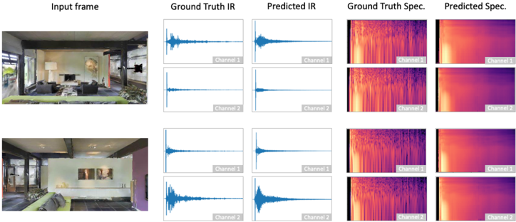## B RIR Prediction Case Study Figure 7: IR Prediction: The first column is the input frame to the encoder. The second column depicts the ground truth IR for the frame and the fourth column is the corresponding spectrogram of this IR. The third and fifth columns show the predicted IR waveform and spectrogram, respectively. This predicted IR waveform is estimated from the spectrogram generated by our network. <details> <summary>Image 7 Details</summary>  ### Visual Description ## Image Comparison: Ground Truth vs. Predicted Room Acoustics ### Overview The image presents a visual comparison between "Ground Truth" (actual) and "Predicted" room acoustics data. It includes input frames (images of rooms), impulse responses (IR), and spectrograms (Spec.) for two different channels. The comparison aims to assess the accuracy of a prediction model in simulating room acoustics. ### Components/Axes * **Titles (Top Row):** * Input frame * Ground Truth IR * Predicted IR * Ground Truth Spec. * Predicted Spec. * **Channel Labels:** Each IR and Spectrogram plot is labeled with either "Channel 1" or "Channel 2" in a gray box at the bottom-right corner. * **Input Frames:** These are images of two different rooms. The first room appears to be a living room with a fireplace, while the second room seems to be a more minimalist space with artwork on the wall. * **Impulse Response (IR) Plots:** These plots show the amplitude of the sound over time. The x-axis represents time, and the y-axis represents amplitude. * **Spectrogram (Spec) Plots:** These plots show the frequency content of the sound over time. The x-axis represents time, and the y-axis represents frequency. The color intensity represents the amplitude of each frequency component. ### Detailed Analysis **Row 1: First Room (Living Room)** * **Input Frame:** A living room scene with a fireplace, seating area, and artwork. * **Ground Truth IR:** * Channel 1: A sharp initial peak followed by a decaying oscillation. * Channel 2: Similar to Channel 1, with a sharp initial peak and decaying oscillation. * **Predicted IR:** * Channel 1: Visually similar to the Ground Truth IR for Channel 1. * Channel 2: Visually similar to the Ground Truth IR for Channel 2. * **Ground Truth Spec:** * Channel 1: Shows a broad range of frequencies with varying intensities over time. The intensity is higher at lower frequencies. * Channel 2: Similar to Channel 1, with a broad range of frequencies and higher intensity at lower frequencies. * **Predicted Spec:** * Channel 1: Appears less detailed than the Ground Truth Spec, with a smoother representation of frequency content. * Channel 2: Similar to Channel 1, less detailed than the Ground Truth Spec. **Row 2: Second Room (Minimalist Room)** * **Input Frame:** A minimalist room with artwork on the wall and a seating area. * **Ground Truth IR:** * Channel 1: A sharp initial peak followed by a decaying oscillation. * Channel 2: Similar to Channel 1, with a sharp initial peak and decaying oscillation. * **Predicted IR:** * Channel 1: Visually similar to the Ground Truth IR for Channel 1. * Channel 2: Visually similar to the Ground Truth IR for Channel 2. * **Ground Truth Spec:** * Channel 1: Shows a broad range of frequencies with varying intensities over time. The intensity is higher at lower frequencies. * Channel 2: Similar to Channel 1, with a broad range of frequencies and higher intensity at lower frequencies. * **Predicted Spec:** * Channel 1: Appears less detailed than the Ground Truth Spec, with a smoother representation of frequency content. * Channel 2: Similar to Channel 1, less detailed than the Ground Truth Spec. ### Key Observations * The predicted impulse responses (IR) appear to closely match the ground truth IRs for both rooms and both channels. * The predicted spectrograms (Spec) are less detailed than the ground truth spectrograms, suggesting that the prediction model may be simplifying the frequency content of the room acoustics. * Both ground truth spectrograms show higher intensity at lower frequencies. ### Interpretation The data suggests that the prediction model is reasonably accurate in predicting the overall impulse response of the rooms. However, the model seems to struggle with capturing the finer details of the frequency content, as evidenced by the less detailed predicted spectrograms. This could be due to limitations in the model's architecture, training data, or the complexity of accurately simulating room acoustics. The model seems to perform consistently across both rooms and channels. The higher intensity at lower frequencies in the spectrograms is a common characteristic of room acoustics, indicating that lower frequencies tend to persist longer in enclosed spaces. </details> We perform a case study on the task of predicting the binaural IR directly from a single visual frame. This helps us evaluate if it is feasible to learn this information just from a visual frame, so that it can be then used for our task as in Sec. 3.2 of the main paper. We predict the acoustic properties of the room by looking at one snapshot of the scene. We predict the magnitude spectrogram of the IR for the two channels. We also obtain the predicted waveform of the IR using the Griffin-Lim algorithm [26]. Figure 7 shows qualitative examples of predictions from the test set. It can be seen that we can get a fairly accurate general idea of the IR, and the difference between the response in each channel is also captured. To evaluate if we capture the materials and geometry effectively, we train another task to predict the reverberation time RT 60 of the IR from the visual frame. A more accurate prediction of RT 60 means that our network understands how the wave will interact with the room and materials and whether it takes more or less time to decay. We formulate this as a classification task and discretize the range of the RT 60 into 10 classes, each with roughly equal number of samples. We then use a classifier to predict this range class of RT 60 using only the visual frame as input. The classifier, consisting of a ResNet-18, has a test accuracy of 61.5% which demonstrates the networks' ability to estimate the RT 60 range quite well. 4 http://vision.cs.utexas.edu/projects/geometry-aware-binaural ## C SimBinaural dataset details To construct the dataset, we insert diverse 3D models of various instruments like guitar, violin, flute etc. and other sound-making objects like phones and clocks into the scene. Each object has multiple models of that class for diversity, so we do not associate a sound with a particular 3D model. We have a total of 35 objects from 11 classes. To generate realistic binaural sound in the environment as if it is coming from the source location and heard at the camera position, we convolve the appropriate SoundSpaces [7] room impulse response with an anechoic audio waveform (e.g., a guitar playing for an inserted guitar 3D object). We use sounds recorded in anechoic environments, so there is no existing reverberations to affect the data. The sounds are obtained from Freesound [17] and OpenAIR data [36] to form a set of 127 different sound clips spanning the 11 distinct object categories. Using this setup, we capture videos with simulated binaural sound. The virtual camera and attached microphones are moved along trajectories such that the object remains in view, leading to diversity in views of the object and locations within each video clip. Using ray tracing, we ensure that the object is in view of the camera, and the source positions are densely sampled from the 3D environments. For a particular video, we use a fixed source position and the agent traverses a random path. The view of the object changes throughout the video as the camera moves and rotates, so we get diverse orientations of the object and positions within a video frame, for each video. The camera moves to a new position every 5 seconds and has a small translational motion during the five-second interval. The videos are generated at 5 frames per second, the average length of the videos in the dataset is 30.3s and the median length is 20s. ## D Implementation Details All networks are written in PyTorch [40]. The backbone network is based upon the networks used for 2.5D visual sound [23] and APNet [63]. The visual network is a ResNet-18 [27] with the pooling and fully connected layers removed. The U-Net consists of 5 convolution layers for downsampling and 5 upconvolution layers in the upsampling network and include skip connections. The encoder for spatial coherence follows the same architecture as the U-Net encoder for the audio feature extraction. The classifier combines the audio and visual features and uses a fully connected layer for prediction. The generator network is adapted from GANSynth [15], modified to fit the required dimensions of the audio spectrogram. To preprocess both datasets, we follow the standard steps from [23]. We resampled all the audio to 16kHz and computed the STFT using a FFT size of 512, window size of 400, and hop length of 160. For training the backbone, we use 0.63s clips of the 10s audio and the corresponding frame. Frames are extracted at 10fps. The visual frames are randomly cropped to 448 × 224. For testing, we use a sliding window of 0.1s to compute the binaural audio for all methods. We use the Adam optimizer [30] and a batch size of 64. The initial learning rates are 0.001 for the audio and fusion networks, and 0.0001 for all other networks. We trained the FAIR-Play dataset for 1000 epochs and SimBinaural for 100 epochs. We train the RIR prediction separately and use the weights for initialization while training jointly. The d for choice of frame is set to 1s and the l 's used are set based on validation set performance to l B = 10 , l S = 1 , l G = 0 . 01 , l P = 1. Table 4: Results on SimBinaural Position-Split with different combinations of constraints. | Method | STFT | ENV | |-------------------|--------|-------| | Spatial+Geometric | 0.724 | 0.118 | | IR Pred+Geometric | 0.707 | 0.117 | | IR Pred+Spatial | 0.702 | 0.117 | ## E Additional Ablations Table 2 in the main paper illustrates that adding each component of our method individually to the visual features helps improve the binaural audio quality performance. Table 4 provides additional analysis to evaluate the combination of different constraints with the backbone for the SimBinaural Position-Split. The constraints complement each other to learn better visual features, leading to better audio performance.