2112.10664v1

## Proving Theorems using Incremental Learning and Hindsight Experience Replay Eser Ayg¨ un DeepMind eser@deepmind.com Laurent Orseau DeepMind lorseau@deepmind.com Xavier Glorot DeepMind glorotx@deepmind.com Vlad Firoiu DeepMind vladfi@deepmind.com Doina Precup DeepMind doinap@deepmind.com Ankit Anand DeepMind anandank@deepmind.com Lei M. Zhang DeepMind lmzhang@deepmind.com Shibl Mourad DeepMind shibl@deepmind.com ## Abstract Traditional automated theorem provers for first-order logic depend on speed-optimized search and many handcrafted heuristics that are designed to work best over a wide range of domains. Machine learning approaches in literature either depend on these traditional provers to bootstrap themselves or fall short on reaching comparable performance. In this paper, we propose a general incremental learning algorithm for training domainspecific provers for first-order logic without equality, based only on a basic given-clause algorithm, but using a learned clause-scoring function. Clauses are represented as graphs and presented to transformer networks with spectral features. To address the sparsity and the initial lack of training data as well as the lack of a natural curriculum, we adapt hindsight experience replay to theorem proving, so as to be able to learn even when no proof can be found. We show that provers trained this way can match and sometimes surpass state-of-the-art traditional provers on the TPTP dataset in terms of both quantity and quality of the proofs. ## 1 Introduction I believe that to achieve human-level performance on hard problems, theorem provers likewise must be equipped with soft knowledge, in particular soft knowledge automatically gained from previous proof experiences. I also suspect that this will be one of the most fruitful areas of research in automated theorem proving. And one of the hardest. Schulz (2017, E's author) Automated theorem proving (ATP) is an important tool both for assisting mathematicians in proving complex theorems as well as for areas such as integrated circuit design, and software and hardware verification (Leroy, 2009; Klein, 2009). Initial research in ATP dates back to 1960s ( e.g. , Robinson (1965); Knuth & Bendix (1970)) and was motivated partly by the fact that mathematics is a hallmark of human intelligence. However, despite significant research effort and progress, ATP systems are still far from human capabilities (Loos et al., 2017). The highest performing ATP systems ( e.g. , Cruanes et al. (2019); Kov´ acs & Voronkov Preprint. Under review. (2013)) are decades old and have grown to use an increasing number of manually designed heuristics, mixed with some machine learning, to obtain a large number of search strategies that are tried sequentially or in parallel. Recent advances (Loos et al., 2017; Chvalovsk` y et al., 2019) build on top of these provers and used modern machine learning techniques to augment, select or prioritize their heuristics, with some success. However, these machinelearning based provers usually require initial training data in the form of proofs, or positive and negative examples (provided by the high-performing existing provers) from which to bootstrap. Recent works do not build on top of other provers, but still require existing proof examples ( e.g. , Goertzel (2020); Polu & Sutskever (2020)). Our perspective is that the reliance of current machine learning techniques on high-end provers limits their potential to consistently surpass human capabilities in this domain. Therefore, in this paper we start with only a basic theorem proving algorithm, and develop machine learning methodology for bootstrapping automatically from this prover. In particular, given a set of conjectures without proofs, our system trains itself, based on its own attempts and (dis)proves an increasing number of conjectures, an approach which can be viewed as a form of incremental learning. A particularly interesting recent advance is rlCop (Kaliszyk et al., 2018; Zombori et al., 2020), which is based on the minimalistic leanCop theorem prover (Otten & Bibel, 2003), and is similar in spirit to our approach. It manages to surpass leanCop's performance-but falls short of better competitors such as E, likely because it is based on a 'tableau' proving style rather than a saturation-based one. This motivated Crouse et al. (2021) to build on top of a saturation-based theorem prover and indeed see some improvement, while still not quite getting close to E. However, all previous approaches using incremental learning have a blind spot, because they learn exclusively from the proofs of successful attempts: If the given set of conjectures have large gaps in their difficulties, the system may get stuck at a suboptimal level due to the lack of new training data. This could in principle even happen at the very start, if all theorems are too hard to bootstrap from. To tackle this issue, Ayg¨ un et al. (2020) propose to create synthetic theorem generators based on the axioms of the actual conjectures, so as to provide a large initial training set with diverse difficulty. Unfortunately, synthetic theorems can be very different from the target conjectures, making transfer difficult. In this paper, we adapt instead hindsight experience replay (HER) (Andrychowicz et al., 2017) to ATP: clauses reached in proof attempts are turned into goals in hindsight. This generates a large amount of 'auxiliary' theorems with proofs for the learner, even when no theorem from the original set can be proven. We compare our approach on a subset of TPTP (Sutcliffe, 2017) with the state-of-the-art E prover (Schulz, 2002; Cruanes et al., 2019), which performs very well on this dataset. Our learning prover eventually reaches equal or better performance on 16 domains out of 20. In addition, it finds shorter proofs than E in approximately 98% of the cases. We perform an ablation experiment to highlight specifically the role of hindsight experience replay. In the next sections, we explain our incremental learning methodology with hindsight experience replay, followed by a description of the network architecture and experimental results. ## 2 Methodology For the reader unfamiliar with first-order logic, we give a succinct primer in Appendix A. From an abstract viewpoint, in our setting the main object under consideration is the clause , and two operations, factoring and resolution . These operations produce more clauses from one or two parent clauses. Starting from a set of axiom clauses and negated conjecture clauses (which we will call input clauses ), the two operations can be composed sequentially to try to reach the empty clause , in which case its ancestors form a refutation proof of the input clauses and correspond to a proof of the non-negated conjecture. We call the tree\_size of a clause the number of symbols (with repetition) appearing in the clause; for example tree\_size ( p ( X,a,X,b ) ∨ q ( a )) is 7. Westart by describing the search algorithm, which allows us then to explain how we integrate machine learning and to describe our overall incremental learning system. ## 2.1 Search algorithm To assess the incremental learning capabilities of recent machine learning advances, we have opted for a simple base search algorithm (see also Kaliszyk et al. (2018) for example), instead of jump-starting from an existing high-performance theorem prover. Indeed, E is a state-of-art prover that incorporates a fair number of heuristics and optimizations (Schulz, 2002; Cruanes et al., 2019), such as: axiom selection, simplifying the axioms and input clauses, more than 60 literal selection strategies, unit clause rewriting, multiple fast indexing techniques, clause evaluation heuristics (tree size preference, age preference, preference toward symbols present in the conjecture, watch lists, etc.), strategy selection based on the analysis of the prover on similar problems, multiple strategy scheduling with 450 strategies tuned on TPTP 7.3.0, 1 integration of a PicoSAT solver, etc. Other machine learning provers based on E ( e.g. , Jakub˚ uv et al. (2020); Loos et al. (2017)) automatically take advantage of at least some of these improvements (but see also Goertzel (2020)). Like E and many other provers, we use a variant of the DISCOUNT loop (Denzinger et al., 1997), itself a variant of the given-clause algorithm (McCune & Wos, 1997) (See Algorithm 3 in Appendix B). The input clauses are initially part of the candidates , while the active\_clauses list starts empty. A candidate clause is selected at each iteration. New factors of the clause, as well as all its resolvents with the active clauses are pushed back into candidates . The given clause is then added to active\_clauses , and we say that it has been processed . We also use the standard forward and backward subsumptions, as well as tautology deletion, which allow to remove too-specific clauses that are provably unnecessary for refutation. If candidates becomes empty before the empty clause can be produced, the algorithm returns "saturated" , which means that the input clauses are actually countersatisfiable (the original conjecture is dis-proven). Given-clause-based theorem provers often use several priority queues to sort the set of candidates ( e.g. , McCune & Wos (1997); Schulz (2002); Kov´ acs & Voronkov (2013)). We also use three priority queues: the age queue, ordered from the oldest generated clause to the youngest, the weight queue, ordered by increasing tree\_size of the clauses, and the learnedcost queue, which uses a neural network to assign a score to each generated clause. The age queue ensures that every generated clause is processed after a number of steps that is at most a constant factor times its age. The weight queue ensures that small clauses are processed early, as they are 'closer' to the empty clause. The learned-cost queue allows us to integrate machine learning into the search algorithm, as detailed below. ## 2.2 Clause-scoring network and hindsight experience replay The clause-scoring network can be trained in many ways so as to find proofs faster. A method utilized by Loos et al. (2017) and Jakubuv & Urban (2019) turns the scoring task into a classification task: a network is trained to predict whether the clause to be scored will appear in the proof or not. In other words, the probability predicted by an 'in-proofness' classifier is used as the score. To train, once a proof is found, the clauses that participate in the proof ( i.e. , the ancestors of the empty clause) are considered to be positive examples, while all other generated clauses are taken as negative examples. 2 Then, given as input one such generated clause x along with the input clauses C s , the network must learn to predict whether x is part of the (found) proof. There are two main drawbacks to this approach. First, if all conjectures are too hard for the initially unoptimized prover, no proof is found and no positive examples are available, making supervised learning impossible. Second, since proofs are often small (often a few dozen steps), only few positive examples are generated. As the number of available conjectures is often small too, there is far too little data to train a modern high-capacity neural network. Moreover, for supervised learning to be successful, the conjectures that can be proven must be sufficiently diverse, so the learner can steadily improve. Unfortunately, there is no 1 See http://www.tptp.org/CASC/J10/SystemDescriptions.html#E---2.5 . 2 These examples are technically not necessarily negative, as they may be part of another proof. But avoiding these examples during the search still helps the system to attribute more significance to the positive examples. guarantee that such a curriculum is available. If the difficulty suddenly jumps, the learner may be unable to improve further. These shortcomings arise because the learner only uses successful proofs, and all the unsuccessful proof attempts are discarded. In particular, the overwhelming majority of the generated clauses become negative examples, and most need to be discarded to maintain a good balance with the positive examples. To leverage the data generated in unsuccessful proof attempts, we adapt the concept of hindsight experience replay (HER) (Andrychowicz et al., 2017) from goal-conditioned reinforcement learning to theorem proving. The core idea of HER is to take any 'unsuccessful' trajectory in a goal-based task and convert it into a successful one by treating the final state as if it were the goal state, in hindsight. A deep network is then trained with this trajectory, by contextualizing the policy with this state instead of the original goal. This way, even in the absence of positive feedback, the network is still able to adapt to the domain , if not to the goal, thus having a better chance to reach the goal on future tries. Inspired by HER, we use the clauses generated during any proof attempt as additional conjectures, which we call hindsight goals , leading to a supply of positive and negative examples. Let D be any non-input clause generated during the refutation attempt of C s . We call D a hindsight goal . 3 Then, the set C s ∪{¬ D } can be refuted. Furthermore, once the prover reaches D starting from C s ∪ {¬ D } , only a few more resolution steps are necessary to reach the empty clause; that is, there exists a refutation proof of C s ∪ {¬ D } where D is an ancestor of the empty clause. Hence, we can use the ancestors of D as positive examples for the negated conjecture and axioms C s ∪ {¬ D } . This generates a very large number of examples, allowing us to effectively train the neural network, even with only a few conjectures at hand. Since each domain has its own set of axioms, and a separate network is trained per domain, axioms are not provided as input to the scoring network. Although the set of active clauses is an important factor in determining the usefulness of a clause, we ignore it in the network input to keep the network size smaller. ## 2.3 Incremental learning algorithm Typical supervised learning ATP systems require a set of proofs (provided by other provers) to optimize their model ( e.g. , Loos et al. (2017); Jakub˚ uv et al. (2020); Ayg¨ un et al. (2020)). Success is assessed by cross-validation. In contrast, we formulate ATP as an incremental learning problem-see in particular Orseau & Lelis (2021); Jabbari Arfaee et al. (2011). Given a pool of unproven conjectures, the objective is to prove as many as possible, even using multiple attempts, and ideally as quickly as possible. Hence, the learning system must bootstrap directly from initially-unproven conjectures, without any initial supervised training data. Success is assessed by the number of proven conjectures, and the time spent solving them. Hence, we do not need to split the set of conjectures into train/test/validate sets because, if the system overfits to the proofs of a subset of conjectures, it will not be able to prove more conjectures. Our incremental learning system is described in Algorithm 1. Initially, all conjectures are unproven and the clause-scoring network is initialized randomly. At this stage, we have no information on how long it takes to prove a certain conjecture, or whether it can be proven at all. The prover attempts to prove all conjectures provided using a scheduler (described below), so as to vary time limits for each conjecture. This ensures that proofs for easy conjectures are obtained early, and the resulting positive and negative examples are then used to train the clause-scoring network. As the network learns, more conjectures can be proven, providing in turn more data, and so on. This incremental learning algorithm thus allows us to automatically build a capable prover for a given domain, starting from a basic prover that may not even be able to prove a single conjecture in the given set. Time scheduling. All conjectures are attempted in parallel, each on a CPU. For each conjecture, we use the uniform budgeted scheduler (UBS) algorithm (Helmert et al., 2019, 3 Note that, while the original version of HER (Andrychowicz et al., 2017) only uses the last reached state as a single hindsight goal, we use all intermediate clauses, providing many more data points. Algorithm 1 Distributed incremental learning. launch starts a new process in parallel. For each conjecture an instance of UBS decides the sequence of time limits for solving attempts. ``` Algorithm 1 Distributed incremental learning. launch starts a new process in parallel. For each conjecture an instance of UBS decides the sequence of time limits for solving attempts. def main(conjectures): # Launch and connect learners, actors and manager with example buffer & task queue example_buffer = create_example_buffer() task_queue = create_task_queue() learners = [for i = 1..10: launch learner(example_buffer)] for i = 1..1000: launch actor(task_queue, learners, example_buffer) actor_manager = launch actor_manager(conjectures, task_queue) wait for actor_manager to finish def learner(example_buffer): repeat forever: # Sample a batch of examples and train the network. batch = sample_batch_uniformly(example_buffer) minimize_classification_loss(batch) # we use cross-entropy def actor(task_queue, learners, example_buffer) repeat forever: # Fetch a task and attempt to prove the conjecture. conjecture, time_limit = get_task(task_queue) learner = sample_uniformly(learners) call search(conjecture) for at most time_limit seconds # see Alg. 3 Appendix B and obtain generated_clauses examples = sample_examples(generated_clauses) # see Alg. 2 put_examples(example_buffer, examples) def actor_manager(conjectures, task_queue): schedulers = [] for conjecture in conjectures: schedulers[conjecture] = initialize_UBS() # see Section 2.3 repeat until all conjectures have been proven: # Choose a random conjecture and enqueue it. conjecture = sample_uniformly(conjectures) scheduler = schedulers[conjecture] time_limit = get_next_time_limit(scheduler) put_task(task_queue, (conjecture, time_limit)) ``` section 7) to further simulate running in (pseudo-)parallel the solver with varying time budgets, and restarting each time the budget is exhausted. In the terminology of UBS, we take T ( k, r ) = 3 r 2 k -1 in seconds, but we cap k ≤ k max = 10. A UBS instance simulates on a single CPU running k max restarting programs, by interleaving them: On a 'virtual' CPU of index k ∈ { 1 , . . . , k max } , a program corresponds to running the prover for a budget of 3 · 2 k -1 seconds before restarting it for the same budget of time and so on; r is the number of restarts. Hence, as the network learns, each conjecture is incrementally attempted with time budgets of varying sizes (3s, 6s, 12s, . . . , 3072s), using no more than one hour, while carefully balancing the cumulative time spent within each budget (Luby et al., 1993; Helmert et al., 2019). Once a proof has been found for a conjecture, the scheduler is not stopped, so as to continue searching for more (often shorter) proofs. Distributed implementation. Our implementation consists of multiple actors running in parallel, a manager that distributes tasks to the actors using the time scheduling algorithm, and a task queue that handles manager-actors communication. We used ten learners training ten separate models to increase the diversity of the search without having to increase the number of actors. These learners are fed with training examples from the actors and use them to update their parameters of their clause-scoring networks. Note that during the first Algorithm 2 Example sampling algorithm. ``` Algorithm 2 Example sampling algorithm. def sample_examples(generated_clauses): # Estimate the number of examples that can be consumed by the learner target_num_examples = time_elapsed_since_last_attempt × target_num_examples_per_second # Remove the input clauses hindsight_goals = generated_clauses \ input_clauses # Subsample the goals and the examples examples = [] sizes = {tree_size(c) : c ∈ hindsight_goals} for size in sizes: size_goals = {c ∈ hindsight_goals : tree_size(c) == size} w_size = 1 / ln(size + e) - 1 / ln(size + e + 1) # See Appendix C num_examples = ceil(target_num_examples × w_size) for _ in range(num_examples): goal = uniform_sample(size_goals) # pick hindsight goal of this size anc = ancestors(goal) examples += [positive_example(uniform_sample(anc), goal)] examples += [negative_example(uniform_sample(hindsight_goals \ anc), goal)] return examples ``` 1 000 updates, the actors do not use the clause-scoring network as its outputs are mostly random. 4 Subsampling hindsight goals and examples. With HER, the number of available examples is actually far too large: if, after a proof attempt, n clauses have been generated ( n may be in the thousands), not only can each clause be used as a hindsight goal, but there are about n 2 pairs (positive example, hindsight goal), and far more negative examples. This suddenly puts us in a very data-rich regime, which contrasts with the data scarcity of learning only from proofs of the given conjecture. Hence, we need to subsample the examples to prevent overwhelming the learner (see Algorithm 2 in the appendix). To this end, we first estimate the number of examples the learner can consume per second before sampling. But there is an additional difficulty: the number of possible clauses is exponentially large in the tree\_size of the clause, while small clauses are likely more relevant since the empty clause (which is the true target) has size 0. Moreover, clauses can be rather large: a tree\_size over 300 is quite common, and we observed some tree\_size over 6 000. To correct for this, we fix the proportion of positive and negative examples for each hindsight goal clause size, ensuring that small hindsight goal clauses are favoured, while allowing a diverse sample of large clauses, using a heavy-tail distribution w s described in Appendix C. Finally, all the positive and negative examples thus sampled are added to the training pool for the learners. 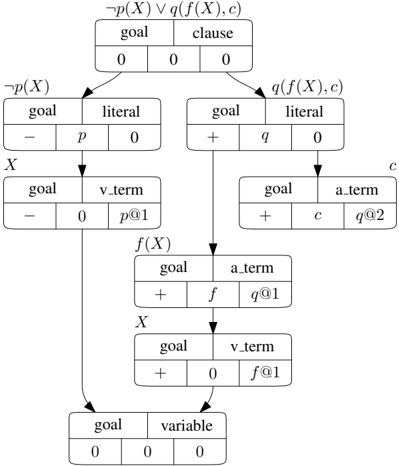## 2.4 Representation Our clause scoring network receives as input the clause to score, x , the hindsight goal clause, g , and a sequence of negated conjecture clauses C s . Individual clauses are transformed to directed acyclic graphs (an example is depicted in Figure 1) with five different node types. First, there is a clause node, whose children are literal nodes, corresponding to all literals of the clause (each one is associated with a predicate). The children of literal nodes represent the arguments of the predicate; they are either variable-term nodes if the argument is a variable, or atomic-term nodes otherwise 5 . Children of atomic-term nodes follow the same description. Finally, each variable-term node is linked to a variable node, which has as many parents as there are instances of the corresponding variable in the clause. 4 We picked 1000 as it appeared to be approximately the number of steps required for the learner to reach the base prover performance on a few experiments. 5 A constant argument is equivalent with a function of arity 0. Figure 1: Clause graph of a goal clause. Each node has five features: clause type, node type, literal polarity, symbol hash and argument slot hash. The parts of formula corresponding to each node are shown outside of the nodes. <details> <summary>Image 1 Details</summary>  ### Visual Description ## Flowchart Diagram: Logical Formula Decomposition ### Overview The diagram represents a hierarchical decomposition of a logical formula, illustrating relationships between variables, literals, clauses, and goals. It uses arrows to denote dependencies and transformations, with boxes containing symbolic logic expressions and numerical values. ### Components/Axes - **Top Box**: - Label: `¬p(X) ∨ q(f(X), c)` - Subcomponents: - `goal`: `0` - `clause`: `0` - `0` (value) - Arrows point to two child boxes: 1. Left: `¬p(X)` 2. Right: `q(f(X), c)` - **Left Branch (`¬p(X)`)**: - Box 1: - `goal`: `-` - `literal`: `p` - `0` (value) - Box 2: - `goal`: `-` - `v_term`: `p@1` - `0` (value) - **Right Branch (`q(f(X), c)`)**: - Box 1: - `goal`: `+` - `literal`: `q` - `0` (value) - Box 2: - `goal`: `+` - `a_term`: `c` - `q@2` (value) - **Intermediate Boxes**: - `f(X)`: - `goal`: `+` - `a_term`: `f` - `q@1` (value) - `X`: - `goal`: `+` - `v_term`: `f@1` - `0` (value) - **Bottom Box**: - `goal`: `0` - `variable`: `0` - `0` (value) ### Detailed Analysis - **Logical Structure**: - The top formula `¬p(X) ∨ q(f(X), c)` is split into two branches via disjunction (`∨`). - The left branch (`¬p(X)`) introduces negation (`-`) and a variable term (`p@1`). - The right branch (`q(f(X), c)`) uses conjunction (`+`) and includes a function application (`f(X)`) and constant (`c`). - **Symbolic Values**: - `0` appears frequently, likely representing "false" or "no contribution." - `+` and `-` denote logical operators (conjunction/disjunction). - `@1` and `@2` may indicate variable instances or positional markers. - **Flow Direction**: - Arrows flow downward from the top formula to subcomponents, suggesting a top-down decomposition. - Variables (`X`, `f(X)`, `c`) are linked to their respective terms (`p@1`, `q@1`, `q@2`). ### Key Observations 1. **Hierarchical Decomposition**: The diagram breaks down a complex formula into atomic components (variables, literals, clauses). 2. **Logical Operators**: The use of `+` and `-` suggests a formal system (e.g., propositional logic or a knowledge base). 3. **Variable Instantiation**: `@1` and `@2` imply multiple instances of variables, possibly for substitution or evaluation. 4. **Goal Values**: The `goal` field in each box may represent evaluation priorities or constraints. ### Interpretation This diagram likely models a logical reasoning process, such as: - **Automated Theorem Proving**: Decomposing a formula into subgoals for evaluation. - **Knowledge Representation**: Structuring relationships between variables, functions, and constants. - **Constraint Satisfaction**: Tracking how variables and literals contribute to satisfying a formula. The repeated use of `0` and `+`/`-` suggests a binary evaluation system, where components are either "active" (`+`) or "inactive" (`-`). The flow from the top formula to variables indicates a dependency chain, where higher-level goals depend on lower-level variable assignments. **Notable Patterns**: - The right branch (`q(f(X), c)`) introduces more complexity with function application and constants. - The bottom box’s `goal: 0` may signify a terminal state or unresolved condition. **Underlying Logic**: The diagram reflects a formal system where logical formulas are recursively broken into evaluable units. The use of `@` notation implies variable binding or substitution, critical in automated reasoning or symbolic computation. </details> To each node, we associate a feature vector composed of the following five components: (i) A one-hot vector of length 3, encoding if the node belongs to x , g or a member of C s . (ii) A one-hot vector of length 5 encoding the node type: clause, literal, atomic-term, variable-term or variable. (iii) A one-hot vector of length 2 encoding if the node belongs to a positive or negative literal (null vector for clause and variable nodes). (iv) A hash vector representing the predicate name or the function/constant name respectively for predicate or atomic-term nodes (null vector for other nodes). (v) A hash vector representing the predicate/function argument slot in which the term is present (null vector for clause, literal and variable nodes). Hash vectors are randomly sampled uniformly on the 64 dimensional unit hyper-sphere, using the name of the predicate, function or constant (and the argument position for slots) as seed. The node feature vectors are projected into a 64-dimensional node embedding space using a linear layer that trains during learning. We use a Transformer encoder architecture (Vaswani et al., 2017) for the clause-scoring network, whose input is composed of the set of node embeddings in the current clause x , goal clause g and conjecture clauses C s , up to 128 nodes. For each node, we compute a spectral encoding vector representing its position in the clause graph (Dwivedi & Bresson, 2020); this is given by the eigenvectors of the Laplacian matrix of the graph from which we keep only the 64 first dimensions, corresponding to the low frequency components. It replaces the traditional positional encoding of Transformers. Note that if there are more than 128 nodes in the set of clause graphs, we prioritize x , then g and C s . Within each graph, we order the nodes from top to bottom then left to right (e.g. the first nodes to be filtered out would be variable- or atomic-term nodes of the last conjecture clause). We only keep the transformer encoder output corresponding to the root node of the target clause and project it, using a linear layer, into a single logit, representing the probability that x will be used to reach g starting from C s . ## 3 Experiments To evaluate our approach, we use the Thousands of Problems for Theorem Proving (TPTP) library (Sutcliffe, 2017) version 7.5.0. We focus on FOF and CNF domains without the equality predicate (those which use the symbol =) that refer to axioms files and contain Table 1: Number of conjectures proven on the twenty domains. E results at the one hour mark (1h) are shown in addition to the E results at the full seven day mark (7d). | Domain | Conjectures | Basic | IL w/o HER | IL w/HER | E (1h) | E (7d) | |----------|---------------|---------|--------------|------------|----------|----------| | FLD1 | 135 | 9 | 12 | 66 | 69 | 75 | | FLD2 | 143 | 6 | 8 | 86 | 87 | 97 | | GEO6 | 164 | 86 | 164 | 164 | 164 | 164 | | GEO7 | 38 | 36 | 38 | 38 | 38 | 38 | | GEO9 | 37 | 37 | 37 | 37 | 37 | 37 | | GRP5 | 10 | 6 | 10 | 10 | 10 | 10 | | KRS1 | 41 | 9 | 37 | 41 | 40 | 40 | | LCL3 | 65 | 33 | 60 | 60 | 60 | 60 | | LCL4 | 168 | 35 | 120 | 155 | 134 | 153 | | MED1 | 9 | 0 | 0 | 9 | 9 | 9 | | NUM1 | 10 | 9 | 9 | 9 | 9 | 9 | | NUM9 | 36 | 4 | 9 | 19 | 25 | 25 | | PLA1 | 26 | 3 | 26 | 26 | 26 | 26 | | PUZ4 | 7 | 1 | 2 | 5 | 4 | 4 | | SET1 | 11 | 6 | 11 | 11 | 11 | 11 | | SWB2 | 6 | 3 | 3 | 6 | 4 | 6 | | SWB3 | 3 | 3 | 3 | 3 | 3 | 3 | | SYN1 | 199 | 199 | 199 | 199 | 199 | 199 | | SYN2 | 7 | 4 | 4 | 4 | 5 | 5 | | TOP1 | 1 | 1 | 1 | 1 | 1 | 1 | | Total | 1116 | 490 | 753 | 949 | 935 | 972 | 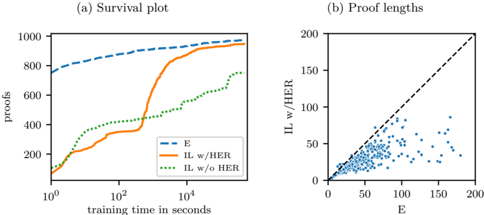Figure 2: (a) Survival plot showing the progress of E and incremental learning with and without hindsight experience replay over the course of seven days of training. The time scale is logarithmic. (b) Scatter plot of the shortest proof lengths achieved by E vs. incremental learning with hindsight experience replay on the conjectures that can be proven by both. <details> <summary>Image 2 Details</summary>  ### Visual Description ## Survival Plot and Proof Lengths Scatter Plot ### Overview The image contains two side-by-side plots analyzing the performance of different proof systems over training time. The left plot (a) shows proof accumulation over time, while the right plot (b) compares proof lengths between two systems. ### Components/Axes **Plot (a) - Survival Plot** - **X-axis**: Training time in seconds (log scale: 10⁰ to 10⁴) - **Y-axis**: Number of proofs (linear scale: 0 to 1000) - **Legend**: - Dashed blue line: E - Solid orange line: IL w/HER - Dotted green line: IL w/o HER - **Legend Position**: Bottom-right corner **Plot (b) - Proof Lengths** - **X-axis**: E (linear scale: 0 to 200) - **Y-axis**: IL w/HER (linear scale: 0 to 200) - **Data Points**: Blue scatter points - **Legend**: Top-right corner (blue points labeled "IL w/HER") - **Diagonal Reference**: Dashed black line (y=x) ### Detailed Analysis **Plot (a) Trends**: 1. **E (dashed blue)**: Steady linear increase from ~800 proofs at 10⁰s to ~950 proofs at 10⁴s 2. **IL w/HER (solid orange)**: - Slow start (10⁰-10¹s: ~100→200 proofs) - Sharp acceleration after 10¹s (200→800 proofs at 10³s) - Plateaus near 950 proofs by 10⁴s 3. **IL w/o HER (dotted green)**: - Gradual increase from ~100→500 proofs over 10⁴s - Shows periodic fluctuations (e.g., ~300→400→500 between 10²-10³s) **Plot (b) Distribution**: - Blue points cluster below the y=x line (IL w/HER < E) - Median E value: ~100 (IL w/HER: ~75) - Outlier region: 10-20 points above y=x line (IL w/HER > E) - Density gradient: Higher concentration of points in lower-left quadrant ### Key Observations 1. HER inclusion (IL w/HER) achieves 2-3x more proofs than IL w/o HER by 10⁴s training time 2. HER reduces average proof length by ~25% compared to E (plot b) 3. IL w/o HER shows diminishing returns after 10³s training time 4. 5% of IL w/HER proofs exceed E's length (potential edge cases) ### Interpretation The data demonstrates that HER (Hereditary Elimination Rule) significantly improves proof generation efficiency: - **Quantity**: HER systems reach near-saturation proof counts faster (orange line vs green) - **Quality**: HER proofs are consistently shorter (plot b scatter below diagonal) - **Tradeoffs**: 5% of HER proofs are longer than E's, suggesting potential optimization opportunities - **Scalability**: E maintains linear growth while HER systems plateau, indicating different convergence behaviors The relationship between proof quantity and length suggests HER enables more proofs without sacrificing (and often improving) proof conciseness, with room for further optimization in exceptional cases. </details> less than 1 000 axioms. This results in 20 domains, named after the corresponding axioms files. Note that the GEO6 and GEO8 axiom files often appear together, and we group them into the GEO6 domain. The resulting list of domains and conjectures can be found in the supplementary material. We ran our incremental learning algorithm with hindsight experience replay (IL w/HER) for seven days on the twenty domains. For each domain, we trained ten models using 1000 actors. We logged every successful attempt that lead to a proof during training, along with the time elapsed, the number of clauses generated, the length of the proof, and the proof itself. In order to show the importance of HER in achieving the results above, we ran the same experiments without HER (IL w/o HER), training the clause-scoring network using solely the data extracted from proofs found for the input problems. To compare our results to the state-of-the-art, we also ran the E prover (Cruanes et al., 2019) version 2.5 on each of the conjectures in the same domains, in 'auto' and 'auto-schedule' modes and with time limits of 2 days, 4 days and 7 days. We then took the union of all solved conjectures from these runs, so as to give E the best shot possible, and because E's behaviour is sensitive to the given time limit. As we never run our prover longer than one hour at a time, we measured E's performance at the one hour mark in addition to the full seven day mark. The hyperparameters used in all experiments are given in Appendix D. Conjectures proven. Table 1 shows the number of conjectures proven by our basic prover (without the learned-cost queue), IL w/o HER, IL w/HER, E at one hour mark (E 1h), and E at full seven day mark (E 7d), as well as the actual number of conjectures, in each domain and in total. According to these results, IL w/HER proved 1.94 times as many problems as the basic prover, improving its performance by almost a factor of two. It proved 14 (1.5%) more conjectures than E 1h and 23 (2.42%) fewer conjectures than E 7d. It outperformed E 7d on three of the domains and matching its performance on 13 of the domains. Nine of the proofs found by IL w/HER were missed by E, which implies that the combination of these provers are better than either of them. Without hindsight. IL w/o HER performed significantly worse, failing to prove 198 (20.9%) of the conjectures that can be proven by IL w/HER. As expected, most of the failures happened in the 'hard' domains, where the basic prover was not performing well. Without enough proofs from which to learn, IL w/o HER stalled and showed little to no progress on these domains. Training vs. searching. In Figure 2a, a comparison of the progress of E and the improvement of our systems can be seen as a survival plot over seven days of run time (wall-clock). Unlike E, which performed up to seven days of proof search per conjecture but has been under constant development for almost two decades, IL w/HER spent the same seven days to train provers based on a simple proof search algorithm from scratch, and ended up finding almost as many proofs as E. Quality of proofs. We also looked at the individual proofs discovered by both systems. Incremental learning combined with the revisiting of previously proven conjectures allowed our system to discover shorter proofs continually. On average, proofs got 13% shorter after their initial discovery. We also observed that the shortest proofs found by our system were shorter than those found by E. Out of the 941 conjectures proven by both systems, our proofs were shorter for 921 conjectures (97.9%) whereas E's proofs were shorter for only 9 conjectures (0.956%) with 11 proofs being of the same length. Figure 2b shows a scatter plot of the lengths of the shortest proofs found by E vs. found by IL w/HER. Speed of search. E was able to perform the proof search 25.6 times faster than our provers in terms of clauses generated per second. We believe that the only way for our system to compete with E under these conditions is to find scoring functions that are as strong as the numerous heuristics built into E for these domains. ## 4 Conclusion In this work, we provide a method for training domain-specific theorem provers given a set of conjectures without proofs. Our proposed method starts from a very simple given-clause algorithm and uses hindsight experience replay (HER) to improve, prove an increasing number of conjectures in incremental fashion. We train a transformer network using spectral features in order to provide a useful scoring function for the prover. Our comparison with the state-of-the-art heuristic-based prover E demonstrates that our approach achieves comparable performance to E, while our proofs are almost always shorter than those generated by E. To our knowledge, the provers trained by our system are the only ones that use machine learning to match the performance of a state-of-the-art first-order logic prover without already being based on one . The experiments also demonstrate that HER allows the learner to improve more smoothly than when learning from proven conjectures alone. We believe that HER is a very desirable component of future ATP/ML systems. Providing more side information to the transformer network, so as to make decisions more context-aware, should lead to further significant improvements. More importantly, while classical first-order logic is a large and important formalism in which many conjectures can be expressed, various other formal logic systems have been developed which are either more expressive or more adapted to different domains (temporal logic, higher-order logic, FOL with equality, etc.). It would be very interesting to try our approach on domains from these logic systems. While the given-clause algorithm and possibly the input representation for the neural networks would need to be adapted, the rest of our methodology is sufficiently general to be used with other logic systems, and still be able to deal with domains without known proofs. ## Acknowlegements We would like to thank Tara Thomas and Natalie Lambert for helping us in planning our research goals and keeping our research focused during the project. We are also grateful to Stephen Mcaleer, Koray Kavukcuoglu, Oriol Vinyals, Alex Davies and Pushmeet Kohli for the helpful discussions during the course of this work. We would also like to thank Stephen Mcaleer, Dimitrios Vytiniotis and Abbas Mehrabian for providing suggestions which helped in improving the manuscript substantially. ## Reproducibility Statement The details of how the dataset is created and divided in different domains is explained in Section 3. Additionally, we include the list of problem files and axiom files used in each domain in the attached supplementary material. The variant of DISCOUNT algorithm is provided in appendix B. The heavy tail distribution used to sample the hindsight goals is provided in appendix C. The details of the hyperparameters used for all the experiments are included in appendix D. The training code was written in JAX (Bradbury et al., 2018). For training, we use 1 CPU for each actor and 1 NVIDIA V100 GPU for each learner. ## References - Marcin Andrychowicz, Filip Wolski, Alex Ray, Jonas Schneider, Rachel Fong, Peter Welinder, Bob McGrew, Josh Tobin, OpenAI Pieter Abbeel, and Wojciech Zaremba. Hindsight experience replay. In Advances in Neural Information Processing Systems , volume 30. Curran Associates, Inc., 2017. - Eser Ayg¨ un, Zafarali Ahmed, Ankit Anand, Vlad Firoiu, Xavier Glorot, Laurent Orseau, Doina Precup, and Shibl Mourad. Learning to prove from synthetic theorems. arXiv preprint arXiv:2006.11259 , 2020. - James Bradbury, Roy Frostig, Peter Hawkins, Matthew James Johnson, Chris Leary, Dougal Maclaurin, George Necula, Adam Paszke, Jake VanderPlas, Skye Wanderman-Milne, and Qiao Zhang. JAX: composable transformations of Python+NumPy programs, 2018. URL http://github.com/google/jax . - Karel Chvalovsk` y, Jan Jakub˚ uv, Martin Suda, and Josef Urban. Enigma-ng: efficient neural and gradient-boosted inference guidance for e. In International Conference on Automated Deduction , pp. 197-215. Springer, 2019. - Maxwell Crouse, Ibrahim Abdelaziz, Bassem Makni, Spencer Whitehead, Cristina Cornelio, Pavan Kapanipathi, Kavitha Srinivas, Veronika Thost, Michael Witbrock, and Achille Fokoue. A deep reinforcement learning approach to first-order logic theorem proving. Proceedings of the AAAI Conference on Artificial Intelligence , 35(7):6279-6287, 2021. - Simon Cruanes, Stephan Schulz, and Petar Vukmirovi´ c. Faster, Higher, Stronger: E 2.3. In TACAS 2019 , volume 11716 of LNAI , pp. 495-507, April 2019. - J¨ org Denzinger, Martin Kronenburg, and Stephan Schulz. Discount - a distributed and learning equational prover. J. Autom. Reason. , 18(2):189-198, 1997. - Vijay Prakash Dwivedi and Xavier Bresson. A generalization of transformer networks to graphs. CoRR , abs/2012.09699, 2020. - Peter Elias. Universal codeword sets and representations of the integers. IEEE Transactions on Information Theory , 21(2):194-203, 1975. - Melvin Fitting. First-order logic and automated theorem proving . Springer Science & Business Media, 2012. - Zarathustra Amadeus Goertzel. Make E smart again (short paper). In Automated Reasoning , pp. 408-415. Springer International Publishing, 2020. - Malte Helmert, Tor Lattimore, Levi H. S. Lelis, Laurent Orseau, and Nathan R. Sturtevant. Iterative budgeted exponential search. In Proceedings of the 28th International Joint Conference on Artificial Intelligence , pp. 1249-1257. AAAI Press, 2019. - S. Jabbari Arfaee, S. Zilles, and R. C. Holte. Learning heuristic functions for large state spaces. Artificial Intelligence , 175(16-17):2075-2098, 2011. - Jan Jakub˚ uv, Karel Chvalovsk` y, Miroslav Olˇ s´ ak, Bartosz Piotrowski, Martin Suda, and Josef Urban. Enigma anonymous: Symbol-independent inference guiding machine (system description). In International Joint Conference on Automated Reasoning , pp. 448-463. Springer, 2020. - Jan Jakubuv and Josef Urban. Hammering Mizar by Learning Clause Guidance (Short Paper). In 10th International Conference on Interactive Theorem Proving (ITP 2019) , volume 141, pp. 34:1-34:8. Schloss Dagstuhl-Leibniz-Zentrum fuer Informatik, 2019. - Cezary Kaliszyk, Josef Urban, Henryk Michalewski, and Miroslav Olˇ s´ ak. Reinforcement learning of theorem proving. In Advances in Neural Information Processing Systems , volume 31. Curran Associates, Inc., 2018. - Diederik P. Kingma and Jimmy Ba. Adam: A method for stochastic optimization. In 3rd International Conference on Learning Representations, ICLR 2015, San Diego, CA, USA, May 7-9, 2015, Conference Track Proceedings , 2015. - Gerwin Klein. Operating system verification-an overview. Sadhana , 34(1):27-69, 2009. - Donald E. Knuth and Peter B. Bendix. Simple word problems in universal algebras. In Computational Problems in Abstract Algebra , pp. 263-297. Pergamon, 1970. - Laura Kov´ acs and Andrei Voronkov. First-order theorem proving and vampire. In International Conference on Computer Aided Verification , pp. 1-35. Springer, 2013. - Xavier Leroy. Formal verification of a realistic compiler. Communications of the ACM , 52 (7):107-115, 2009. - Sarah Loos, Geoffrey Irving, Christian Szegedy, and Cezary Kaliszyk. Deep network guided proof search. In LPAR-21. 21st International Conference on Logic for Programming, Artificial Intelligence and Reasoning , volume 46 of EPiC Series in Computing , pp. 85105, 2017. - Michael Luby, Alistair Sinclair, and David Zuckerman. Optimal speedup of Las Vegas algorithms. Inf. Process. Lett. , 47(4):173-180, September 1993. - William McCune and Larry Wos. Otter - the CADE-13 competition incarnations. Journal of Automated Reasoning , 18(2):211-220, 1997. - Laurent Orseau and Levi H. S. Lelis. Policy-guided heuristic search with guarantees. Proceedings of the AAAI Conference on Artificial Intelligence , 35(14):12382-12390, May 2021. - Jens Otten and Wolfgang Bibel. leancop: lean connection-based theorem proving. Journal of Symbolic Computation , 36(1):139-161, 2003. - Stanislas Polu and Ilya Sutskever. Generative language modeling for automated theorem proving. arXiv preprint arXiv:2009.03393 , 2020. - J. A. Robinson. A machine-oriented logic based on the resolution principle. J. ACM , 12(1): 23-41, 1965. - Stephan Schulz. E-a brainiac theorem prover. AI Communications , 15(2, 3):111-126, 2002. - Stephan Schulz. We know (nearly) nothing! But can we learn? In ARCADE 2017. 1st International Workshop on Automated Reasoning: Challenges, Applications, Directions, Exemplary Achievements , volume 51 of EPiC Series in Computing , pp. 29-32. EasyChair, 2017. - Geoff Sutcliffe. The TPTP Problem Library and Associated Infrastructure. From CNF to TH0, TPTP v6.4.0. Journal of Automated Reasoning , 59(4):483-502, 2017. - Ashish Vaswani, Noam Shazeer, Niki Parmar, Jakob Uszkoreit, Llion Jones, Aidan N Gomez, /suppress L ukasz Kaiser, and Illia Polosukhin. Attention is all you need. In Advances in Neural Information Processing Systems , volume 30. Curran Associates, Inc., 2017. - Zsolt Zombori, Josef Urban, and Chad E Brown. Prolog technology reinforcement learning prover. In International Joint Conference on Automated Reasoning , pp. 489-507. Springer, 2020. ## A A quick primer on first-order logic and resolution calculus First-order logic (FOL) is a formal language used to express mathematical or logical statements. We give a brief introduction to first-order logic here. For more information, see (Fitting, 2012). Any statement expressed in first-order logic is called first-order logic formula. For example the statement: 'for all people X,Y and Z , if X is a parent of Y and Y is a parent of Z , then X is grandparent of Z ' can be expressed as the FOL formula: ∀ X, ∀ Y, ∀ Z, parent( X,Y ) ∧ parent( Y, Z ) ⇒ grandparent( X,Z ). Here, X,Y,Z are variables , and parent and grandparent are predicates . We will only consider FOL formulas expressed in Conjunctive Normal Form (CNF), as a conjunction ( ∧ ) of clauses , in which all variables are implicitly universally quantified ( ∀ ). Consider the following CNF formula: $$\underbrace { ( \neg p a r e n t ( X , Y ) \vee \neg p a r e n t ( Y , Z ) \vee g r a n d p a r e n t ( X , Z ) ) } _ { C _ { 1 } } \wedge \underbrace { p a r e n t ( a l i c e , b o b ) } _ { C _ { 2 } } \wedge \underbrace { p a r e n t ( b o b , c h a r l i e ) } _ { C _ { 3 } }$$ A clause is a disjunction ( ∨ ) of a number of literals ; we will also consider clauses to be sets of literals to simplify the notation. C 1 , C 2 and C 3 are clauses. Note that C 1 is equivalent to the first FOL formula example above, expressed as a clause. A literal is an atom , possibly preceded by the negation ¬ , in which case it is a negative literal (positive otherwise). For example, parent( X,Y ) and ¬ parent( Y, Z ) are literals. An atom is a predicate name of arity n ∈ N followed by a list of n terms . A term is either a function name of associated arity n ∈ N followed by a list of n terms, or a constant (such as alice, bob), or a variable . We assume that two different clauses of the same formula cannot share variables. A clause C is a tautology if C contains both a literal /lscript and its negation ¬ /lscript . Tautologies can be safely removed from a CNF formula without changing its truth value. The tree\_size of a clause is the number is the number of nodes when the clause is represented as a tree of terms. For example, tree\_size (parent( X, bob)) is 3. A substitution is a set { V 1 t 1 , V 2 t 2 , . . . } where V 1 , V 2 , . . . are variables and t 1 , t 2 , . . . are terms. The set of variables { V 1 , V 2 , . . . } is the domain of the substitution. The application σ ( C ) of a substitution σ to a clause C (or also to a single literal) results in a new clause C ′ = σ ( C ) where all occurrences of the variables (of the domain of σ ) in C are replaced with their corresponding terms according to the substitution σ . For example, if C = parent( X,Y ) and σ = { X alice , Y Z } then σ ( C ) = parent(alice , Z ). Two literals /lscript 1 and /lscript 2 can be unified if there exists a substitution σ such that applying it to both literals result in the same literal, that is, σ ( /lscript 1 ) = σ ( /lscript 2 ). In such a case, the most general unifier mgu( /lscript 1 , /lscript 2 ) of /lscript 1 and /lscript 2 is the smallest substitution that unifies the two literals, and it is unique (up to a renaming of the variables). For example, the most general unifier of C = parent( X,Y ) and C ′ = parent(alice , Z ) is { X alice , Y Z } , such that σ ( C ) = σ ( C ′ ) = parent(alice , Z ). A clause C 1 subsumes a clause C 2 if there exists a substitution σ such that σ ( C 1 ) ⊆ C 2 where the clauses are considered to be sets of literals. 6 For example the clause p ( X,a ) subsumes the clause p ( b, a ) ∨ p ( c, a ), with σ = { X b } (or also with σ = { X c } ) as σ ( { p ( X,a ) } ) ⊆ { p ( b, a ) , p ( c, a ) } . The clause C ′ is a factor of a clause C if there exist a substitution σ and two literals /lscript and /lscript ′ in C such that σ = mgu( /lscript, /lscript ′ ) and C ′ = σ ( C \ { /lscript } ). The operation factoring( C ) returns the set of all factors (unique up to renaming of the variables) of C , with 'fresh' (never used) variables. For example, we can factor C 1 on its first two literals to obtain the clause ¬ parent( Y ′ , Y ′ ) ∨ grandparent( Y ′ , Y ′ ) with the substitution { X Y, Z Y } . A clause is the sole parent of its factors. The clause C ′′ is a resolvent of two clauses C and C ′ if there exist a substitution σ , a positive literal /lscript in C and a negative literal /lscript ′ in C ′ such that σ = mgu( /lscript, /lscript ′ ) and C ′′ = σ ( C \ { /lscript } ∪ C ′ \ { /lscript ′ } ). The operation resolution( C, C ′ ) produces the set of all possible resolvents of C and C ′ (Robinson, 1965), with 'fresh' variables. For example, the resolvents of C 1 and C 2 are {¬ parent(bob , Z ′ ) ∨ grandparent(alice , Z ′ ) , ¬ parent( X ′ , alice) ∨ grandparent( X ′ , bob) } . 6 We assume that syntactic duplicate literals are removed automatically. The clauses C and C ′ are called the parents of C ′′ . The ancestors of a clause are its parents, the parents of its parents and so on. Together, resolution and factoring are sound and also sufficient for refutation completeness , that is, they can only produce clauses that are logically implied by the initial clauses, and if the empty clause is logically implied by the initial clauses, then the empty clause can be also be produced by a sequence of resolution and factoring operations starting from the initial clauses. For example, suppose that we want to prove that alice is the grandparent of someone, that is, that grandparent(alice , A ) can be satisfied for some value of A . Then we negate this conjecture to obtain the clause (implicitly universally quantified over A ) with a single literal: C 4 = ¬ grandparent(alice , A ) and we attempt to refute the CNF formula C 1 ∧ · · · ∧ C 4 , that is, to reach the empty clause using resolution and factoring. First we can resolve C 4 with C 1 to obtain C 5 = ¬ parent(alice , Y ′ ) ∨ ¬ parent( Y ′ , A ′ ). Then we can resolve C 5 with C 2 to obtain C 6 = ¬ parent(bob , A ′′ ) and finally we can resolve C 6 with C 3 to obtain the empty clause, which means that indeed alice is the grandparent of someone. ## B Our DISCOUNT-like algorithm Our simple search algorithm is given in Algorithm 3. See the main text for more details. Algorithm 3 Our variant of the DISCOUNT algorithm. Note that we use three priority queues for the candidates (see main text). ``` def ``` ``` Algorithm 3 Our variant of the DISCOUNT algorithm. Note that we use three priority queues for the candidates (see main text). <code><loc_1><loc_50><loc_499><loc_498><_Python_>def search(input_clauses) candidates = input_clauses active_clauses = {} # Saturation loop. while candidates is not empty: given_clause = extract_best_clause(candidates) if given_clause is empty_clause: return "refuted" if tautology(given_clause): continue # discard the given_clause for c in active_clauses: if c.subsumes given_clause: continue # forward subsumption if given_clause.subsumes c: active_clauses.remove(c) # backward # Generate factors and resolvents. candidates.append(given_clause.factors()) for c in active_clauses: candidates.append(resolve(given_clause, c)) active_clauses.insert(given_clause) return "saturated" ``` ## C A heavy-tail distribution over the integers To ensure a preference for smaller clauses, while ensuring some diversity of the clause sizes, we use the following heavy-tail distribution for s ∈ { 0 , 1 , 2 . . . } : $$w _ { s } = 1 / \ln ( s + e ) - 1 / \ln ( s + e + 1 ) \, .$$ These weights constitute a telescoping series and ensure that ∑ ∞ s =0 w s = 1 while, using ln(1 + 1 /x ) ≥ 1 / ( x +1), $$w _ { s } = \frac { \ln \left ( 1 + \frac { 1 } { s + e } \right ) } { \ln ( s + e ) \ln ( s + e + 1 ) } \geq \frac { 1 } { ( s + e + 1 ) ( \ln ( s + e + 1 ) ) ^ { 2 } } \, .$$ Thus, w is a heavy-tailed universal distribution over the nonnegative integers in the sense that -ln w s ∈ O (ln s ), similarly to Elias' delta coding (Elias, 1975). Tangentially, sampling according to w s is simple since its cumulative distribution telescopes: Sample u uniformly in [0 , 1], then select the integer min { s ≥ 0 : 1 -1 / ln( s + e +1) ≥ u } , that is, select s = /ceilingleft exp(1 / (1 -u )) -e -1 /ceilingright . ## D Hyperparameters For the transformer encoder, hyperparameter notations from Vaswani et al. (2017) are given in parenthesis for reference. The model is trained using stochastic gradient descent with the Adam optimizer (Kingma & Ba, 2015) with β 1 = 0.9, β 2 = 0.999 and /epsilon1 = 10 -8 . A subset of hyper-parameters have been selected by running the model on the FLD1 domain, selected values are underlined: number of layers ( N ) in { 3, 4, 5 } , embedding size ( d k , d v ) in { 64, 128, 256 } , hash vector size in { 16, 64, 256 } , learning rate in { 0.003, 0.001, 0.0003 } , probability of dropout ( P drop ) in { 0., 0.1, 0.2, 0.3, 0.5, 0.7 } . The other hyperparameters were fixed: the batch size is 2560, the number of attention heads ( h ) is 8, which leads to a dimensionality ( d model ) of 512, the inner-layers have a dimensionality ( d FF ) of 1024. To ensure diversity in the training examples, learners wait for the experience replay buffer to contain at least 65536 examples and then sample uniformly from it. The learners used Nvidia V100s GPUs with 16GB of memory. For the actors, the age, weight, and learned-cost queues in our given-clause algorithm are selected on average 1/13th, 3/13th and 9/13th of the steps, respectively. The batch size is set at 320. All actors and E are limited at 8GB of memory on modern AMD 64bit platforms.