# Long Story Short: Omitted Variable Bias in Causal Machine Learning
**Authors**: Victor Chernozhukov, Carlos Cinelli, Whitney Newey, Amit Sharma, Vasilis Syrgkanis
Abstract.
We develop a general theory of omitted variable bias for a wide range of common causal parameters, including (but not limited to) averages of potential outcomes, average treatment effects, average causal derivatives, and policy effects from covariate shifts. Our theory applies to nonparametric models, while naturally allowing for (semi-)parametric restrictions (such as partial linearity) when such assumptions are made. We show how simple plausibility judgments on the maximum explanatory power of omitted variables are sufficient to bound the magnitude of the bias, thus facilitating sensitivity analysis in otherwise complex, nonlinear models. Finally, we provide flexible and efficient statistical inference methods for the bounds, which can leverage modern machine learning algorithms for estimation. These results allow empirical researchers to perform sensitivity analyses in a flexible class of machine-learned causal models using very simple, and interpretable, tools. We demonstrate the utility of our approach with two empirical examples.
Keywords: sensitivity analysis, short regression, long regression, omitted variable bias, Riesz representation, omitted confounders, causal models, machine learning, confidence bounds.
† Dept. of Economics, Massachusetts Institute of Technology, Cambridge, MA, USA. Email: vchern@mit.edu
* Dept. of Statistics, University of Washington, Seattle, WA, USA. Email: cinelli@uw.edu
‡ Dept. of Economics, Massachusetts Institute of Technology, Cambridge, MA, USA. Email: wnewey@mit.edu
$\|$ Microsoft Research India, Bangalore, India. Email: amshar@microsoft.com
§ Dept. of Mgmt Science and Engineering, Stanford University, Stanford, CA, USA. Email: vsyrgk@stanford.edu
Date: May 26, 2024. First ArXiv version: December 2021. This is an extended version of an earlier paper prepared for the NeurIPS-21 Workshop “Causal Inference & Machine Learning: Why now?”. We thank Isaiah Andrews, Elias Bareinboim, Ben Deaner, David Green, Judith Lok, Esfandiar Maasoumi, Steve Lehrer, Richard Nickl, Anna Miksusheva, Jack Porter, James Poterba, Eric Tchetgen Tchetgen, Ingrid Van Keilegom, and also participants of the Chambelain seminar, Canadian Economic Association the Institute for Nonparametric, and Uncertainty in Artificial Intelligence meetings, and seminars at Harvard-MIT, Wisconsin, Emory, Berkeley Methods Workshop, and BU Causal Seminar for very helpful comments. We are grateful to Jack Porter for suggesting the “long story short” title. This work was partially funded by the Royalty Research Fund at the University of Washington. R package for the methods developed in this paper is available at https://github.com/carloscinelli/dml.sensemakr. R and Python implementations are also available via the DoubleML ecosystem at https://docs.doubleml.org/stable/index.html.
1. Introduction
Unmeasured confounding is a pervasive issue in studies that aim to draw causal inferences from observational data. Such studies typically rely on a conditional ignorability (also known as unconfoundedness) assumption, which states that the treatment assignment is independent of potential outcomes given a set of observed covariates (Rosenbaum and Rubin, 1983a; Pearl, 2009; Angrist and Pischke, 2009; Imbens and Rubin, 2015). This assumption, however, requires that there are no unobserved confounders influencing both the treatment and the outcome. When such variables are omitted from the analysis, empirical estimates may differ from the true causal effect of interest, giving rise to what is now commonly known as “omitted variable bias.”
The omitted variable bias (OVB) problem is one the most significant threats to the identification of causal effects. In the context of linear models, this bias amounts to the difference between the coefficients of the treatment variable from two distinct outcome regressions: one that controls only for observed covariates (the “short” regression) and another that would additionally control for unobserved variables (the “long” regression). Formulas characterizing this difference play a foundational role in statistics, econometrics, and related fields (see, e.g., discussions in classical and modern textbooks, such as Goldberger, 1991; Angrist and Pischke, 2009 and Wooldridge, 2010). Such results allow empirical analysts to understand and bound the maximum size of the bias, by making plausibility judgments on the magnitude of parameters that comprise the OVB formula.
But while linear models are widely used in applied work, they are often overly restrictive. For example, in the binary treatment case, using linear models when treatment effects are heterogeneous may yield unintuitive or even misleading estimates of the causal effects of interest (Aronow and Samii, 2016; Słoczyński, 2022). To address these limitations, many empirical analysts have turned their attention to more flexible nonlinear or nonparametric models, often leveraging modern machine learning techniques for estimation and inference (Van der Laan and Rose, 2011; Belloni et al., 2013; Chernozhukov et al., 2018a; Athey et al., 2019). These tools offer the flexibility to capture complex relationships between variables, avoiding stringent functional form assumptions in causal effect estimation. Yet, we currently lack general OVB results for nonlinear models (whether parametric or nonparametric), as we have for the linear case. Our work provides such results.
In this paper we develop a general theory of omitted variable bias for a wide range of common causal parameters that can be identified as linear functionals of the conditional expectation function (CEF) of the outcome. Such functionals encompass many (if not most) of the traditional targets of investigation in causal inference studies, such as averages of potential outcomes, average treatment effects, average causal derivatives, and policy effects from covariate shifts. We allow for arbitrary treatment (e.g continuous or binary) and outcome variables. Our theory applies to general nonparametric models, while naturally allowing for (semi-)parametric restrictions (such as partial linearity) when such assumptions are made. Our formulation recovers well-known and familiar OVB results for linear models as a special case, and it can be seen as its natural generalization to nonlinear models. Importantly, we show that the general nonparametric bounds on the bias still have a simple and interpretable form.
More specifically, we first formalize the OVB problem in the nonparametric setting. Paralleling the linear case, we define the OVB as the difference between the “short” and “long” functionals of the outcome regression, where the former omits and the latter includes the latent variables. To derive the OVB, our construction then leverages the Riesz-Frechet representation of the target functionals, which allows us to rewrite the parameters of interest as weighted averages of the outcome regression, with weights given by the Riesz representers (RRs). We show that the OVB arises as a by-product of confounders introducing systematic errors in both the outcome regression and in the RRs for the parameter of interest. Furthermore, the bound on the bias has a simple characterization, depending only on the additional variation that latent variables create in the outcome regression and in the RRs. As a result, plausibility judgments on the maximum explanatory power of latent variables suffice to place overall bounds on the bias, simplifying the task of sensitivity analysis even when using nonparametric or otherwise complex models.
Although these general results may initially seem abstract to those not familiar with Riesz representation theory, in many leading examples the RRs in fact correspond to quantities that are well-known to empirical researchers. For instance, when estimating the average treatment effect in a partially linear model, the RR is the (variance scaled) residualized treatment, after “partialling out” the control covariates. Or, when estimating an average treatment effect in a general nonparametric model with a binary treatment, the RR is now given by another familiar quantity—the inverse probability of treatment weights (IPTW). In such cases, we show that the bounds on the bias can be reparameterized in terms of simple percentage gains in variance explained (or precision) in the treatment and the outcome regression due to unmeasured confounders, again facilitating the interpretation and use of the OVB formulas in practice. We further help analysts make plausibility judgments on the magnitude of sensitivity parameters by means of comparison of the relative strength of unobserved confounders against the strength of observed covariates.
Finally, we provide statistical inference for these bounds using debiased machine learning (DML) and auto-DML (Chernozhukov et al., 2018a, b, 2020, 2022c). Our construction makes it possible to use modern machine learning methods for estimating the identifiable components of the bounds, including regression functions, Riesz representers, the norm of regression residuals, and the norm of Riesz representers. These results enables flexible and efficient statistical inference on the bounds, allowing researchers to perform sensitivity analyses against unmeasured confounding in a flexible class of machine-learned causal models using simple and interpretable tools. Here we provide DML-based statistical inference on the bounds, but we note that our approach can also be used with classical parametric and nonparametric estimation methods.
Related Literature
Our work is most closely related to the literature that derives OVB formulas for linear models, such as those found in traditional textbooks and recent extensions (Goldberger, 1991; Angrist and Pischke, 2009; Wooldridge, 2010; Frank, 2000; Oster, 2019; Cinelli and Hazlett, 2020). We advance this literature by providing analogous, easily explainable OVB formulas for a broad and rich class of causal parameters, all for general nonlinear models, with or without further parametric restrictions. Importantly, we provide a single unifying framework that covers all these cases, and that can be easily specialized depending on the target parameter and on whether additional parametric assumptions (if any) are made. We further advance the OVB literature by providing flexible and efficient statistical inference methods, leveraging modern machine learning algorithms with debiased machine learning.
More broadly, our work is related to the extensive literature on sensitivity analysis against unmeasured confounders. Here we highlight the key differences between our approach and existing methods, while relegating a more detailed review to the Appendix, Section D. First, many prior works on sensitivity analysis either focus exclusively on binary treatments (e.g., Rosenbaum, 2002; Tan, 2006; Masten and Poirier, 2018; Kallus et al., 2019; Zhao et al., 2019; Bonvini and Kennedy, 2021), target a single estimand of interest, such as a causal risk ratio (Ding and VanderWeele, 2016; VanderWeele and Ding, 2017), or impose parametric assumptions on the observed data or on the nature of unobserved confounding (Rosenbaum and Rubin, 1983b; Imbens, 2003; Dorie et al., 2016; Cinelli et al., 2019). Our approach differs from these in that (i) it is not limited to binary treatments, (ii) it covers a broader range of target parameters, such as average causal derivatives and average policy effects from covariate shifts, and (iii) it does not require parametric assumptions on the observed data nor on the nature of confounding.
Even if we focus solely on the important special case of estimating an average treatment effect (ATE) with a binary treatment, our OVB results usefully complements other seminal approaches on this problem such as those of Rosenbaum (2002) or the marginal sensitivity models of Tan (2006). Whereas such approaches limit the strength of confounding through its impact on the worst case change that confounders could cause in the odds ratio of treatment assignment—a quantity economists rarely focus on—our approach limits the strength of confounding through its impact on the gains in precision in the treatment regression, a measure of explanatory power similar in nature to a simple $R^{2}$ in a linear model. Moreover, even in stylized models of treatment assignment (e.g, a logistic model with a Gaussian latent confounder), worst-case approaches such as the ones in Rosenbaum (2002) and Tan (2006) have a naturally unbounded sensitivity parameter, no matter how small the actual degree of confounding is, whereas our approach does not suffer from this problem (see Section E of the Appendix for an example).
Our OVB-based approach also differs from traditional sensitivity analyses in that it derives the exact OVB formula for the target parameters we cover. For example, our results show that the bias of the ATE in the binary treatment case is not determined by deviations on the odds of treatment; rather, it is determined by three quantities: (i) the maximum explanatory power of confounders in the treatment regression, as given by gains in precision, (ii) the maximum explanatory power of confounders in the outcome regression, as given by gains in variance explained, and (iii) by the correlation of errors in the regression function and the IPTW. Therefore, beyond being a tool for sensitivity analysis, OVB results such as ours provide a precise characterization of the bias, and reveal that any alternative approach that parameterize deviations from unconfoundedness in a different way can only affect the bias insofar as it constraints these three quantities.
Overview of the paper
Section 2 presents our method in the simpler context of partially linear models. The results in that section serve not only as an accessible introduction to the main ideas of our general framework, but are also important in their own right, since partially linear models are widely used in applied work. Section 3 derives the main results of the paper—we characterize and bound the omitted variable bias for continuous linear functionals of the conditional expectation function of the outcome, based on their Riesz representations, all for general, nonparametric causal models. In Section 4 we construct high-quality inference methods for the bounds on the target parameters by leveraging recent advances in debiased machine learning with Riesz representers. Section 5 demonstrates the use of our tools to assess the robustness of causal claims in a detailed empirical example that estimates the average treatment effect of 401(k) eligibility on net financial assets. Section 6 concludes with suggestions for possible extensions. The Appendix contains all proofs, provides a more extensive literature review, as well as an additional empirical example that illustrates sensitivity analyses for average causal derivatives with continuous treatments.
Notation.
All random vectors are defined on the probability space with probability measure ${\mathrm{P}}$ . We consider a random vector $Z=(Y,W)$ with distribution $P$ taking values $z$ in its support $\mathcal{Z}$ ; we use $P_{V}$ to denote the probability law of any subvector $V$ and $\mathcal{V}$ denote its support. We use $\|f\|_{P,q}=\|f(Z)\|_{P,q}$ to denote the $L^{q}(P)$ norm of a measurable function $f:\mathcal{Z}→\mathbb{R}$ and also the $L^{q}(P)$ norm of random variable $f(Z)$ . For a differentiable map $x\mapsto g(x)$ , from $\mathbb{R}^{d}$ to $\mathbb{R}^{k}$ , $∂_{x^{\prime}}g$ abbreviates the partial derivatives $(∂/∂ x^{\prime})g(x)$ , and $∂_{x^{\prime}}g(x_{0})$ means $∂_{x^{\prime}}g(x)\mid_{x=x_{0}}$ . We use $x^{\prime}$ to denote the transpose of a column vector $x$ ; we use $R^{2}_{U\sim V}$ to denote the $R^{2}$ from the orthogonal linear projection of a scalar random variable $U$ on a random vector $V$ . We use the conventional notation $dL/dP$ to denote the Radon-Nykodym derivative of measure $L$ with respect to $P$ .
2. Warm-Up: Omitted Variable Bias in Partially Linear Models
To fix ideas, we begin our discussion in the context of partially linear models (PLM). These results not only provide the key intuitions and the building blocks for the general case of nonseparable, nonparametric models of Section 3, but they are also important in their own right, as these models are widely used in applied work.
2.1. Problem set-up
Consider the partially linear regression model of the form
$$
Y=\theta D+f(X,A)+\epsilon. \tag{1}
$$
Here $Y$ denotes a real-valued outcome, $D$ a real-valued treatment, $X$ an observed vector of covariates, and $A$ an unobserved vector of covariates. We refer to $W:=(D,X,A)$ as the “long” list of regressors, and to equation (1) as the “long” regression. For exposition purposes, we assume the error term $\epsilon$ obeys ${\mathrm{E}}[\epsilon|D,X,A]=0$ and thus ${\mathrm{E}}[Y|D,X,A]=\theta D+f(X,A)$ , though we note this assumption is not necessary. We can also consider the case where $\theta D+f(X,A)$ is the projection of the CEF on the space of functions that are partially linear in $D$ .
Under the traditional assumption of conditional ignorability, Along with consistency and usual regularity conditions. we have that the regression coefficient $\theta$ identifies the average treatment effect of a unit increase of $D$ on the outcome $Y$ ,
$$
{\mathrm{E}}[Y(d+1)-Y(d)]={\mathrm{E}}[{\mathrm{E}}[Y|D=d+1,X,A]-{\mathrm{E}}[%
Y|D=d,X,A]]=\theta,
$$
where $Y(d)$ denotes the potential outcome of $Y$ when the treatment $D$ is experimentally set to $d$ . The problem, however, is that $A$ is not observed, and thus both the long regression, and the regression coefficient $\theta$ cannot be computed from the available data.
Since the latent variables $A$ are not measured, an alternative route to obtain an approximate estimate of $\theta$ is to consider the partially linear projection of $Y$ on the “short” list of observed regressors $W^{s}:=(D,X)$ , as in,
$$
Y=\theta_{s}D+f_{s}(X)+\epsilon_{s}, \tag{2}
$$
where here we do not make the assumption that the regression is correctly specified, and thus the error term simply obeys the orthogonality condition ${\mathrm{E}}[\epsilon_{s}(D-{\mathrm{E}}[D\mid X])]=0$ . Following convention, we call equation (2) the “short regression.” We can then use the “short” regression parameter $\theta_{s}$ as a proxy for $\theta$ .
Evidently, in general $\theta_{s}$ is not equal to $\theta$ , and this naturally leads to the question of how far our “proxy” $\theta_{s}$ can deviate from the true inferential target $\theta$ . Our goal is, thus, to analyze the difference between the short and long parameters—the omitted variable bias (OVB):
$$
\theta_{s}-\theta,
$$
and perform inference on this bias under various hypotheses on the strength of the latent confounders $A$ .
2.2. OVB as the covariance of approximation errors
Recall that, using a Frisch-Waugh-Lovell partialling out argument, one can express the long and short regression parameters, $\theta$ and $\theta_{s}$ , as the linear projection coefficients of $Y$ on the residuals $D-{\mathrm{E}}[D\mid X,A]$ and $D-{\mathrm{E}}[D\mid X]$ , respectively. That is,
$$
\theta={\mathrm{E}}Y\alpha(W),\quad\quad\theta_{s}={\mathrm{E}}Y\alpha_{s}(W^{%
s}); \tag{3}
$$
where here we define
$$
\alpha(W):=\frac{D-{\mathrm{E}}[D\mid X,A]}{{\mathrm{E}}(D-{\mathrm{E}}[D\mid X%
,A])^{2}},\quad\alpha_{s}(W^{s}):=\frac{D-{\mathrm{E}}[D\mid X]}{{\mathrm{E}}(%
D-{\mathrm{E}}[D\mid X])^{2}}.
$$
For reasons that will become clear in the next section, we can refer to $\alpha(W)$ and $\alpha_{s}(W^{s})$ as the “long” and “short” Riesz representers (RR). We are deliberately introducing Riesz representers in this section to smooth the transition to the general case. The formulation in terms of Riesz representers is a key innovation of this paper and it has not appeared in previous works on omitted variable bias.
Now let $g(W):={\mathrm{E}}[Y\mid D,X,A]$ and $g_{s}(W^{s}):=\theta_{s}D+f_{s}(X)$ denote the long and short regressions, respectively. Using the orthogonality conditions in (1) and (2), we can further express $\theta$ and $\theta_{s}$ as
$$
{\mathrm{E}}Y\alpha(W)={\mathrm{E}}g(W)\alpha(W),\quad\quad{\mathrm{E}}Y\alpha%
_{s}(W^{s})={\mathrm{E}}g_{s}(W^{s})\alpha_{s}(W^{s}). \tag{4}
$$
Our first characterization of the OVB is thus as follows, where we use the shorthand notation: $g=g(W)$ , $g_{s}=g_{s}(W^{s})$ , $\alpha=\alpha(W)$ , and $\alpha_{s}=\alpha_{s}(W^{s})$ .
**Theorem 1 (OVB and Sharp Bounds—PLM)**
*Assume that $Y$ and $D$ are square integrable with:
$$
{\mathrm{E}}(D-{\mathrm{E}}[D\mid X,A])^{2}>0.
$$
Then the OVB for the partially linear model of equations (1) - (2) is given by
$$
\theta_{s}-\theta={\mathrm{E}}(g_{s}-g)(\alpha_{s}-\alpha),
$$
that is, it is the covariance between the regression error and the RR error. Furthermore, the squared bias can be bounded as
$$
|\theta_{s}-\theta|^{2}=\rho^{2}B^{2}\leq B^{2},
$$
where
$$
B^{2}:={\mathrm{E}}(g-g_{s})^{2}{\mathrm{E}}(\alpha-\alpha_{s})^{2},\quad\rho^%
{2}:=\mathrm{Cor}^{2}(g-g_{s},\alpha-\alpha_{s}).
$$
The bound $B^{2}$ is the product of additional variations that omitted confounders generate in the regression function and in the RR. This bound is sharp in the sense that maximizing $\rho^{2}$ over $\alpha$ and $g$ , subject to fixing $B^{2}$ and ${\mathrm{E}}(g-g_{s})^{2}≤{\mathrm{E}}(Y-g_{s})^{2}$ , gives value 1.*
This result for partially linear models is new and it naturally generalizes the traditional OVB formula for linear models. It is worth noting that the proof of Theorem 1 does not rely on the assumption that the long regression is partially linear, even though this assumption was made for expository purposes. In general, if we define both $g$ and $g_{s}$ to be projections of $Y$ onto the space of functions that are partially linear on $D$ , the results of the theorem still hold.
2.3. Further characterization of the bias
Sensitivity analysis requires making plausibility judgments on the values of the sensitivity parameters. Therefore, it is important that such parameters be well-understood, and easily interpretable in applied settings. Here we show how the bias of Theorem 1 can be reparameterized in terms of conventional $R^{2}$ s.
Recall that, when the CEF is not linear, a natural measure of the strength of relationship between some variable $W$ and another variable $V$ is the nonparametric $R^{2}$ —also known as Pearson’s correlation ratio (Pearson, 1905; Doksum and Samarov, 1995):
$$
\eta^{2}_{V\sim W}:=R^{2}_{V\sim{\mathrm{E}}[V|W]}=\operatorname{Var}({\mathrm%
{E}}[V|W])/\operatorname{Var}(V)=\frac{\operatorname{Var}(V)-{\mathrm{E}}[%
\operatorname{Var}(V|W)]}{\operatorname{Var}(V)}.
$$
Further, the nonparametric partial $R^{2}$ of a variable $V$ with another variable $A$ given $X$ measures the additional gain in the explanatory power that $A$ provides, beyond what is already is explained by $X$ . This also equals the relative decrease in the average residual variance:
$$
\eta^{2}_{V\sim A\mid X}:=\frac{\eta^{2}_{V\sim AX}-\eta^{2}_{V\sim X}}{1-\eta%
^{2}_{V\sim X}}=\frac{{\mathrm{E}}[\operatorname{Var}(V|X)]-{\mathrm{E}}[%
\operatorname{Var}(V|X,A)]}{{\mathrm{E}}[\operatorname{Var}(V|X)]}. \tag{5}
$$
We are now ready to rewrite the bound of Theorem 1.
**Corollary 1 (Interpreting OVB Bounds in Terms ofR2superscript𝑅2R^{2}italic_R start_POSTSUPERSCRIPT 2 end_POSTSUPERSCRIPT—PLM)**
*Under the conditions of Theorem 1, we can further express the bound $B^{2}$ as
$$
B^{2}=C^{2}_{Y}C^{2}_{D}S^{2},\quad S^{2}:={\mathrm{E}}(Y-g_{s})^{2}{\mathrm{E%
}}\alpha_{s}^{2}, \tag{6}
$$
where
$$
\quad C^{2}_{Y}=R^{2}_{Y-g_{s}\sim g-g_{s}};\quad C^{2}_{D}:=\frac{1-R^{2}_{%
\alpha\sim\alpha_{s}}}{R^{2}_{\alpha\sim\alpha_{s}}}, \tag{7}
$$
and $1-R^{2}_{\alpha\sim\alpha_{s}}=\eta^{2}_{D\sim A\mid X}$ . Furthermore, if ${\mathrm{E}}[Y|D,X]=\theta_{s}+f_{s}(X)$ , then $R^{2}_{Y-g_{s}\sim g-g_{s}}=\eta^{2}_{Y\sim A\mid DX}.$*
The bound is the product of the term $S^{2}$ , which is directly identifiable (and thus estimable) from the observed distribution of $(Y,D,X)$ , and the term $C^{2}_{Y}C^{2}_{D}$ , which is not identifiable from the data, and needs to be restricted through hypotheses that limit the strength of confounding. The factors $C^{2}_{Y}$ and $C^{2}_{D}$ measure the strength of confounding that the omitted variables generate in the outcome and treatment regressions. More precisely,
- $R^{2}_{Y-g_{s}\sim g-g_{s}}$ ( $=\eta^{2}_{Y\sim A\mid DX}$ under partial linearity of the short regression) in $C^{2}_{Y}$ measures the proportion of residual variation of the outcome explained by latent confounders; and,
- $1-R^{2}_{\alpha\sim\alpha_{s}}=\eta^{2}_{D\sim A\mid X}$ in $C^{2}_{D}$ measures the proportion of residual variation of the treatment explained by latent confounders.
Note how this parameterization simplifies the complexity of plausibility judgments. Researchers now need only to reason about the maximum explanatory power that unobserved confounders have in explaining treatment and outcome variation, as given by familiar $R^{2}$ measures, in order to place bounds on the size of the bias. Finally, in practice, both $\theta_{s}$ and $S^{2}$ need to be estimated from finite samples. This can be readily done using debiased machine learning, as we discuss in Section 4.
3. Main Results: Omitted Variable Bias in Nonparametric Causal Models
We now derive the main results of the paper, and construct sharp bounds on the size of the omitted variable bias for a broad class of causal parameters that can be identified as linear functionals of the conditional expectation function of the outcome. Although more abstract, the presentation of this section largely parallels the special case of partially linear models given in Section 2.
3.1. Problem set-up
As a motivating example, consider the following nonparametric structural equation model (SEM):
| | $\displaystyle Y$ | $\displaystyle=$ | $\displaystyle g_{Y}(D,X,A,\epsilon_{Y}),$ | |
| --- | --- | --- | --- | --- |
where $Y$ is an outcome variable, $D$ is a treatment variable, $X$ is a vector-valued observed confounder variable, $A$ is a vector-valued latent confounder variable, and $\epsilon_{Y},\epsilon_{D},\epsilon_{A}$ are vector-valued structural disturbances that are mutually independent. This model has an associated Directed Acyclic Graph (DAG) (Pearl, 2009) as shown in Figure 1(a).
The SEM above induces the potential outcome $Y(d)$ under the intervention that sets $D$ experimentally to $d$ ,
$$
Y(d):=g_{Y}(d,X,A,\epsilon_{Y}).
$$
The structural model also encodes a consistency assumption between observed and potential outcomes, $Y=Y(D)$ . Additionally, the independence of the structural disturbances implies the following conditional ignorability condition:
$$
Y(d)\perp\!\!\!\!\perp D\mid\{X,A\}, \tag{8}
$$
which states that the realized treatment $D$ is independent of the potential outcomes, conditionally on $X$ and $A$ . More generally, we can work with any causal inference framework that implies the existence of potential outcomes, the consistency of observed and potential outcomes, and such that the conditional ignorability assumption (8) holds (Angrist and Pischke, 2009; Pearl, 2009; Imbens and Rubin, 2015). There are many structural models that satisfy the conditional ignorability assumption (8); see e.g. Pearl (2009) and Figure 1 for concrete examples.
Under this set-up and when $d$ is in the support of $D$ given $X$ , $A$ , we then have the following (well-known) identification result
$$
{\mathrm{E}}[Y(d)\mid X,A]={\mathrm{E}}[Y(d)\mid D=d,X,A]={\mathrm{E}}[Y\mid D%
=d,X,A]=:g(d,X,A),
$$
that is, the conditional average potential outcome coincides with the “long” regression function of $Y$ on $D$ , $X$ , and $A$ . Therefore, we can identify various causal parameters—functionals of the average potential outcome—from the regression function. Important examples include: (i) the average treatment effect (ATE)
$$
\theta={\mathrm{E}}[Y(1)-Y(0)]={\mathrm{E}}[g(1,X,A)-g(0,X,A)], \tag{1}
$$
for the case of a binary treatment $D$ ; and, (ii) the average causal derivative (ACD)
$$
\theta={\mathrm{E}}\left[\partial_{d}{\mathrm{E}}[Y(D)\mid X,A]\right]={%
\mathrm{E}}[\partial_{d}g(D,X,A)],
$$
for the case of a continuous treatment $D$ .
$D$ $Y$ $X$ $A$
(a)
$D$ $Y$ $X$ $A$
(b)
$D$ $Y$ $A_{1}$ $X$ $A_{2}$
(c)
$D$ $Y$ $X_{1}$ $X_{2}$ $A$
(d)
Figure 1. Examples of different DAGs that imply $Y(d)\perp\!\!\!\!\perp D\mid\{X,A\}$ .
Note: Examples of DAGs (nonparametric SEMs) that imply the conditional ignorability condition (8). Latent nodes are circled. DAGs (1(a)) and (1(b)) represent opposite directions $X→ A$ and $A→ X$ , respectively, while yielding the same conditional ignorability condition. DAG (1(c)) shows a special case of (1(b)) by setting $A=(A_{1},A_{2})$ . DAG (1(d)) illustrates the case where we only observe the “negative controls” $X_{1}$ and $X_{2}$ , which are proxies of $A$ . The conditional ignorability condition (8) still holds in this case.
In fact, our framework is considerably more general, and it covers any target parameter of the following form.
**Assumption 1 (Target “Long” Parameter)**
*The target parameter $\theta$ is a continuous linear functional of the long regression:
$$
\theta:={\mathrm{E}}m(W,g); \tag{9}
$$
where the mapping $f\mapsto m(w;f)$ is linear in $f∈ L^{2}(P_{W})$ , and the mapping $f\mapsto{\mathrm{E}}m(W,f)$ is continuous in $f$ with respect to the $L^{2}(P_{W})$ norm.*
This formulation covers the two previous examples with scores $m(W,g)=g(1,X,A)-g(0,X,A)$ for the ATE and $m(W,g)=∂_{d}g(D,X,A)$ for the ACD. The continuity condition holds under the regularity conditions provided in the remark below. We discuss many other examples of this form later in Section 3.4.
**Remark 1 (Regularity Conditions for ATE and ACD)**
*As regularity conditions for the ATE we assume ${\mathrm{E}}Y^{2}<∞$ and the weak overlap condition:
$$
{\mathrm{E}}[P(D=1\mid X,A)^{-1}P(D=0\mid X,A)^{-1}]<\infty.
$$
As regularity conditions for the ACD we assume ${\mathrm{E}}Y^{2}<∞$ , that the conditional density $d\mapsto f(d|x,a)$ is continuously differentiable on its support $\mathcal{D}_{x,a}$ , the regression function $d\mapsto g(d,x,a)$ is continuously differentiable on $\mathcal{D}_{x,a}$ , and we have that $f(d|x,a)$ vanishes whenever $d$ is on the boundary of $\mathcal{D}_{x,a}$ . The above needs to hold for all values $x$ and $a$ in the support of $(X,A)$ . We also impose the bounded information assumption:
$$
{\mathrm{E}}(\partial_{d}\log f(D\mid X,A))^{2}<\infty.
$$
These conditions imply that Assumption 1 holds, by Theorem 3 given in Section 3.4. ∎*
The key problem is that we do not observe $A$ . Therefore we can only identify the “short” conditional expectation of $Y$ given $D$ and $X$ , i.e.
$$
g_{s}(D,X):={\mathrm{E}}[Y\mid D,X].
$$
With the short regression in hand, we can compute proxies (or approximations) $\theta_{s}$ for $\theta$ . In particular, for the ATE, the short parameter consists of
$$
\theta_{s}={\mathrm{E}}[g_{s}(1,X)-g_{s}(0,X)],
$$
and for the ACD,
$$
\theta_{s}={\mathrm{E}}[\partial_{d}g_{s}(D,X)].
$$
In this general framework, the proxy parameter can also be expressed as the same linear functional applied to the short regression, $g_{s}(W^{s})$ .
**Assumption 2 (Proxy “Short” Parameter)**
*The proxy parameter $\theta_{s}$ is defined by replacing the long regression $g$ with the short regression $g_{s}$ in the definition of the target parameter:
$$
\theta_{s}:={\mathrm{E}}m(W,g_{s}).
$$
We require $m(W,g_{s})=m(W^{s},g_{s})$ , i.e., the score depends only on $W^{s}$ when evaluated at $g_{s}$ .*
In the two working examples this assumption is satisfied, since $m(W,g_{s})=m(W^{s},g_{s})=g_{s}(1,X)-g_{s}(0,X)$ for the ATE and $m(W,g_{s})=m(W^{s},g_{s})=∂_{d}g_{s}(D,X)$ for the ACD. Section 3.4 verifies this assumption for other examples.
Our goal is to characterize and provide bounds on the omitted variable bias (OVB), ie., the difference between the “short” and “long” functionals,
$$
\theta_{s}-\theta,
$$
under assumptions that limit the strength of confounding, and perform statistical inference on its size.
3.2. Omitted variable bias for linear functionals of the CEF
The key to bounding the bias is the following lemma that characterizes the target parameters and their proxies as inner products of regression functions with terms called Riesz representers (RR).
**Lemma 1 (Riesz Representation)**
*There exist unique square integrable random variables $\alpha(W)$ and $\alpha_{s}(W^{s})$ , the long and short Riesz representers, such that
$$
\theta={\mathrm{E}}m(W,g)={\mathrm{E}}g(W)\alpha(W),\quad\theta_{s}={\mathrm{E%
}}m(W^{s},g_{s})={\mathrm{E}}g_{s}(W^{s})\alpha_{s}(W^{s}),
$$
for all square-integrable $g$ ’s and $g_{s}$ . Furthermore, $\alpha_{s}(W^{s})$ is the projection of $\alpha$ in the sense that
$$
\alpha_{s}(W^{s})={\mathrm{E}}[\alpha(W)\mid W^{s}].
$$*
In the case of the ATE with a binary treatment, the representers are just the classical inverse probability of treatment (Horvitz-Thompson) weights:
$$
\alpha(W)=\frac{D}{P(D=1\mid X,A)}-\frac{1-D}{P(D=0\mid X,A)},\quad\alpha_{s}(%
W)=\frac{D}{P(D=1\mid X)}-\frac{1-D}{P(D=0\mid X)}.
$$
This follows from change of measure arguments. While it may not be immediately obvious that $\alpha_{s}=E[\alpha|D,X]$ , one can easily show that by applying Bayes’ rule.
In the case of the ACD with a continuous treatment, using integration by parts we can verify that the representers are logarithmic derivatives of the conditional densities:
$$
\alpha(W)=-\partial_{d}\log f(D\mid X,A),\quad\alpha_{s}(W^{s})=-\partial_{d}%
\log f(D\mid X).
$$
We give more involved examples in the next section.
Using this lemma, we obtain the following characterization of the OVB and bounds on its size.
**Theorem 2 (OVB and Sharp Bounds)**
*Consider the long and short parameters $\theta$ and $\theta_{s}$ as given by Assumptions 1 and 2. We then have that the OVB is
$$
\theta_{s}-\theta={\mathrm{E}}(g_{s}-g)(\alpha_{s}-\alpha),
$$
that is, it is the covariance between the regression error and the RR error. Therefore, the squared bias can be bounded as
$$
|\theta_{s}-\theta|^{2}=\rho^{2}B^{2}\leq B^{2},
$$
where
$$
B^{2}:={\mathrm{E}}(g-g_{s})^{2}{\mathrm{E}}(\alpha-\alpha_{s})^{2},\quad\rho^%
{2}:=\mathrm{Cor}^{2}(g-g_{s},\alpha-\alpha_{s}).
$$
The bound $B^{2}$ is the product of additional variations that omitted confounders generate in the regression function and in the RR. This bound is sharp in the sense that maximizing $\rho^{2}$ over $\alpha$ and $g$ subject to fixing $B^{2}$ and ${\mathrm{E}}(g-g_{s})^{2}≤{\mathrm{E}}(Y-g_{s})^{2}$ gives value 1.*
This is the main conceptual result of the paper, and it is new. It covers a rich variety of causal estimands of interest, as long as they can be written as linear functionals of the long regression. We analyze further examples of this class of estimands in Section 3.4.
3.3. Characterization of the OVB bounds
In the same spirit of Section 2, we can further derive useful characterizations of the bounds.
**Corollary 2 (Interpreting OVB Bounds in Terms ofR2superscript𝑅2R^{2}italic_R start_POSTSUPERSCRIPT 2 end_POSTSUPERSCRIPT)**
*The bound of Theorem 2 can be re-expressed as
$$
B^{2}=C^{2}_{Y}C^{2}_{D}S^{2},\quad S^{2}:={\mathrm{E}}(Y-g_{s})^{2}{\mathrm{E%
}}\alpha_{s}^{2}, \tag{10}
$$
where
| | $\displaystyle C^{2}_{Y}$ | $\displaystyle:=$ | $\displaystyle\frac{{\mathrm{E}}(g-g_{s})^{2}}{{\mathrm{E}}(Y-g_{s})^{2}}=R^{2}%
_{Y-g_{s}\sim g-g_{s}},\quad C^{2}_{D}:=\frac{{\mathrm{E}}\alpha^{2}-{\mathrm{%
E}}\alpha^{2}_{s}}{{\mathrm{E}}\alpha^{2}_{s}}=\frac{1-R^{2}_{\alpha\sim\alpha%
_{s}}}{R^{2}_{\alpha\sim\alpha_{s}}}.$ | |
| --- | --- | --- | --- | --- |*
This generalizes the result of Corollary 1 to fully nonlinear models, and general target parameters defined as linear functionals of the long regression. As before, the bound is the product of the term $S^{2}$ , which is directly identifiable from the observed distribution of $(Y,D,X)$ , and the term $C^{2}_{Y}C^{2}_{D}$ , which is not identifiable, and needs to be restricted through hypotheses that limit strength of confounding.
Here, again, the terms $C^{2}_{Y}$ and $C^{2}_{D}$ generally measure the strength of confounding that the omitted variables generate in the outcome regression and in the treatment:
- $R^{2}_{Y-g_{s}\sim g-g_{s}}$ in the first factor measures the proportion of residual variance in the outcome explained by confounders;
- $1-R^{2}_{\alpha\sim\alpha_{s}}$ in the second factor measures the proportion of residual variation of the long RR generated by latent confounders.
Likewise, we have the same useful interpretation of $C^{2}_{Y}$ as the nonparametric partial $R^{2}$ of $A$ with $Y$ , given $D$ and $X$ , namely, $C^{2}_{Y}=\eta^{2}_{Y\sim A\mid D,X}$ . The interpretation of $1-R^{2}_{\alpha\sim\alpha_{s}}$ can be further specialized for different cases, as follows.
**Remark 2 (Interpretation of1−Rα∼αs21subscriptsuperscript𝑅2similar-to𝛼subscript𝛼𝑠1-R^{2}_{\alpha\sim\alpha_{s}}1 - italic_R start_POSTSUPERSCRIPT 2 end_POSTSUPERSCRIPT start_POSTSUBSCRIPT italic_α ∼ italic_α start_POSTSUBSCRIPT italic_s end_POSTSUBSCRIPT end_POSTSUBSCRIPTfor the ATE with a Binary Treatment)**
*For the ATE example, we have that
$$
1-R^{2}_{\alpha\sim\alpha_{s}}=\frac{{\mathrm{E}}[1/\text{Var}(D|X,A)]-{%
\mathrm{E}}[1/\text{Var}(D|X)]}{{\mathrm{E}}[1/\text{Var}(D|X,A)]}\in[0,1]. \tag{11}
$$
That is, $1-R^{2}_{\alpha\sim\alpha_{s}}$ measures the relative gain in the average precision of the treatment model due to $A$ . Precision is the inverse of the variance. Thus, the interpretation of $1-R^{2}_{\alpha\sim\alpha_{s}}$ for the ATE with a binary treatment parallels that of the partially linear model (compare it to equation (5)), with the sole distinction being that, here, gains in predictive power are measured by the relative increase in precision rather than the relative decrease in variance. This connection can be strengthened by considering a latent Gaussian confounder model $D=1(D^{*}>0)$ , where $D^{*}=g(X)-\mu A-\sqrt{1-\mu^{2}}\epsilon_{D},$ with $\epsilon_{D}$ and $A$ both mutually independent standard Gaussian, and also independent of $X$ . Note that $g(X)$ is identified from the relation ${\mathrm{E}}[D\mid X]=\Phi(g(X))$ . Then $P[D=1\mid X,A]=\Phi((g(X)-\mu A)/\sqrt{1-\mu^{2}})$ , and $P[D=1\mid X]=\Phi(g(X))$ , from which the relative gain in precision can be computed. Then here the gain in precision is a monotone function of $\mu^{2}=\eta^{2}_{D^{*}\sim A|X}$ , the $R^{2}$ in the latent regression of $D^{*}$ on $A$ , after adjusting for $X$ . This connection may be useful for empirical work. ∎*
And an analogous interpretation applies for average causal derivatives.
**Remark 3 (Interpretation of1−Rα∼αs21subscriptsuperscript𝑅2similar-to𝛼subscript𝛼𝑠1-R^{2}_{\alpha\sim\alpha_{s}}1 - italic_R start_POSTSUPERSCRIPT 2 end_POSTSUPERSCRIPT start_POSTSUBSCRIPT italic_α ∼ italic_α start_POSTSUBSCRIPT italic_s end_POSTSUBSCRIPT end_POSTSUBSCRIPTfor Average Causal Derivatives)**
*For the ACD example,
$$
1-R^{2}_{\alpha\sim\alpha_{s}}=\frac{{\mathrm{E}}[(\partial_{d}\log f(D\mid X,%
A))^{2}]-{\mathrm{E}}[(\partial_{d}\log f(D\mid X))^{2}]}{{\mathrm{E}}[(%
\partial_{d}\log f(D\mid X,A))^{2}]}\in[0,1], \tag{12}
$$
which can be interpreted as the relative gain in information that the confounder $A$ provides about the location of $D$ . Furthermore, if $D$ is homoscedastic Gaussian, conditional on both $X$ and $(X,A)$ , we then have
$$
\partial_{d}\log f(D\mid X,A)=-\frac{D-{\mathrm{E}}[D\mid X,A]}{{\mathrm{E}}(D%
-{\mathrm{E}}[D\mid X,A])^{2}},\quad\partial_{d}\log f(D\mid X,A)=-\frac{D-{%
\mathrm{E}}[D\mid X]}{{\mathrm{E}}(D-{\mathrm{E}}[D\mid X])^{2}},
$$
so that $1-R^{2}_{\alpha\sim\alpha_{s}}$ simplifies to the nonparametric $R^{2}$ of the latent variable with the treatment, similarly to the partially linear model, i.e, $1-R^{2}_{\alpha\sim\alpha_{s}}=\eta^{2}_{D\sim A|X}$ . ∎*
Beyond making direct plausibility judgments on the strength of confounding using the above quantities, analysts can also leverage judgments of relative importance of variables to bound the size of the bias (see, e.g. Imbens, 2003; Cinelli and Hazlett, 2020). For instance, if one has reasons to believe that $A$ would not generate as much gains in explanatory power as certain key observed covariates $X_{j}$ , this can be used to formally place bounds on the strength of confounding due to $A$ . This allows one to assess, for instance, whether confounders as strong or stronger then observed covariates would be sufficient to overturn an empirical result. We elaborate the benchmarking procedure formally in Section F of the appendix and illustrate its use in the empirical example. These results extend previous benchmarking ideas for linear regression models to the general case.
3.4. Theoretical details for leading causal estimands
We now provide theoretical details for a wide variety of interesting and important causal estimands. Recall that we use $W=(D,X,A)$ to denote the “long” set of regressors and $W^{s}=(D,X)$ to denote the “short” list of regressors.
Let us start with examples for the binary treatment case, with the understanding that finitely discrete treatments can be analyzed similarly.
**Example 1 (Weighted Average Potential Outcome)**
*Let $D∈\{0,1\}$ be the indicator of the receipt of the treatment. Define the long parameter as
$$
\theta={\mathrm{E}}[g(\bar{d},X,A)\ell(W^{s})],
$$
where $w^{s}\mapsto\ell(w^{s})$ is a bounded non-negative weighting function and $\bar{d}$ is a fixed value in $\{0,1\}$ . We define the short parameter as
$$
\theta_{s}={\mathrm{E}}[g_{s}(\bar{d},X)\ell(W^{s})].
$$
We assume ${\mathrm{E}}Y^{2}<∞$ and the weak overlap condition
$$
{\mathrm{E}}[\ell^{2}(W^{s})/P(D=\bar{d}\mid X,A)]<\infty.
$$*
The long parameter is a weighted average potential outcome (PO) when we set the treatment to $\bar{d}$ , under the standard conditional ignorability assumption (8). The short parameter is a statistical approximation based on the short regression. In this example, setting
- $\ell(w^{s})=1$ gives the average PO in the entire population;
- $\ell(w^{s})=1(x∈{\mathcal{N}})/P(X∈\mathcal{N})$ the average PO for group $\mathcal{N}$ ;
- $\ell(w^{s})=1(d=1)/P(D=1)$ the average PO for the treated.
Above we can consider $\mathcal{N}$ as small regions shrinking in volume with the sample size, to make the averages local, as in Chernozhukov et al. (2018b), but for simplicity we take them as fixed in this paper.
**Example 2 (Weighted Average Treatment Effects)**
*In the setting of the previous example, define the long parameter
$$
\theta={\mathrm{E}}[(g(1,X,A)-g(0,X,A))\ell(W^{s})],
$$
and the short parameter as
$$
\theta_{s}={\mathrm{E}}[(g_{s}(1,X)-g_{s}(0,X))\ell(W^{s})].
$$
We further assume ${\mathrm{E}}Y^{2}<∞$ and the weak overlap condition
$$
{\mathrm{E}}[\ell^{2}(W^{s})/\{P(D=0\mid X,A)P(D=1\mid X,A)\}]<\infty.
$$*
The long parameter is a weighted average treatment effect under the standard conditional ignorability assumption. In this example, setting
- $\ell(w^{s})=1$ gives ATE in the entire population;
- $\ell(w^{s})=1(x∈\mathcal{N})/P(X∈\mathcal{N})$ the ATE for group $\mathcal{N}$ ;
- $\ell(w^{s})=1(d=1)/P(D=1)$ the ATE for the treated;
- $\ell(x)=\pi(x)$ the average value of policy (APV) $\pi$ ,
where the policy $\pi$ assigns a fraction $0≤\pi(x)≤ 1$ of the subpopulation with observed covariate value $x$ to receive the treatment.
In what follows $D$ does not need to be binary. We next consider a weighted average effect of changing observed covariates $W^{s}$ according to a transport map $w^{s}\mapsto T(w^{s})$ , where $T$ is deterministic measurable map from $\mathcal{W}^{s}$ to $\mathcal{W}^{s}$ . For example, the policy
$$
(D,X,A)\mapsto(D+1,X,A)
$$
adds a unit to the treatment $D$ , that is $T(W^{s})=(D+1,X)$ . This has a causal interpretation if the policy induces the equivariant change in the regression function, namely the counterfactual outcome $\tilde{Y}$ under the policy obeys ${\mathrm{E}}[\tilde{Y}|X,A]=g(T(W^{s}),A)$ , and the counterfactual covariates are given by $\tilde{W}=(T(W^{s}),A)$ .
**Example 3 (Average Policy Effect from TransportingWssuperscript𝑊𝑠W^{s}italic_W start_POSTSUPERSCRIPT italic_s end_POSTSUPERSCRIPT)**
*For a bounded weighting function $w^{s}\mapsto\ell(w^{s})$ , the long parameter is given by
$$
\theta={\mathrm{E}}[\{g(T(W^{s}),A)-g(W^{s},A)\}\ell(W^{s})].
$$
The short form of this parameter is
$$
\theta_{s}={\mathrm{E}}[\{g_{s}(T(W^{s}))-g_{s}(W^{s})\}\ell(W^{s})].
$$
As the regularity conditions we require that the support of $P_{\tilde{W}}=\mathrm{Law}(T(W^{s}),A)$ is included in the support of $P_{W}$ , and require the weak overlap condition
$$
{\mathrm{E}}[(\ell(dP_{\tilde{W}}-dP_{W})/dP_{W})^{2}]<\infty.
$$*
We now turn to examples with continuous treatments $D$ taking values in $\mathbb{R}^{k}$ . Consider the average causal effect of the policy that shifts the distribution of covariates via the map $W=(D,X,A)\mapsto(T(W^{s}),A)=(D+rt(W^{s}),X,A)$ weighted by $\ell(W^{s})$ , keeping the long regression function invariant. The following long parameter $\theta$ is an approximation to $1/r$ times this average causal effect for small values of $r$ . This example is a differential version of the previous example.
**Example 4 (Weighted Average Incremental Effects)**
*Consider the long parameter taking the form of the average directional derivative:
$$
\theta={\mathrm{E}}[\ell(W^{s})t(W^{s})^{\prime}\partial_{d}g(D,X,A)],
$$
where $\ell$ is a bounded weighting function and $t$ is a bounded direction function. The short form of this parameter is
$$
\theta_{s}={\mathrm{E}}[\ell(W^{s})t(W^{s})^{\prime}\partial_{d}g_{s}(D,X)].
$$
As regularity conditions, we suppose that ${\mathrm{E}}Y^{2}<∞$ . Further for each $(x,a)$ in the support of $(X,A)$ , and each $d$ in $\mathcal{D}_{x,a}$ , the support of $D$ given $(X,A)=(x,a)$ , the derivative maps $d\mapsto∂_{d}g(d,x,a)$ and $d\mapsto g(w)\omega(w)$ , for $\omega(w):=\ell(d,x)t(d,x)f(d|x,a)$ , are continuously differentiable; the set $\mathcal{D}_{x,a}$ is bounded, and its boundary is piecewise-smooth; and $\omega(w)$ vanishes for each $d$ in this boundary. Moreover, we assume the weak overlap:
$$
{\mathrm{E}}[(\mathrm{div}_{d}\omega(W)/f(D|X,A))^{2}]<\infty.
$$*
Another example is that of a policy that shifts the entire distribution of observed covariates, independently of $A$ . The following long parameter corresponds to the average causal contrast of two policies that set the distribution of observed covariates $W^{s}$ to $F_{0}$ and $F_{1}$ , independently of $A$ . Note that this example is different from the transport example, since here the dependence between $A$ and $W^{s}$ is eliminated under the interventions.
**Example 5 (Policy Effect from Changing Distribution ofWssuperscript𝑊𝑠W^{s}italic_W start_POSTSUPERSCRIPT italic_s end_POSTSUPERSCRIPT)**
*Define the long parameter as
$$
\theta=\int\left[\int g(w^{s},a)dP_{A}(a)\right]\ell(w^{s})d\mu(w^{s});\quad%
\mu(w^{s})=F_{1}(w^{s})-F_{0}(w^{s}),
$$
where $\ell$ is a bounded weight function, and the short parameter as
$$
\theta_{s}=\int g_{s}(w^{s})\ell(w^{s})d\mu(w^{s});\quad\mu(w^{s})=F_{1}(w^{s}%
)-F_{0}(w^{s}).
$$
As the regularity conditions we require that the supports of $F_{0}$ and $F_{1}$ are contained in the support of $W^{s}$ , and that the measure $dP_{A}× dF_{k}$ is absolutely continuous with respect to the measure $dP_{W}$ on $\mathcal{A}×\text{support}(\ell)$ . We further assume that ${\mathrm{E}}Y^{2}<∞$ and the weak overlap:
$$
{\mathrm{E}}[(\ell[dP_{A}\times d(F_{1}-F_{0})]/dP)^{2}]<\infty.
$$*
The following result establishes the validity of the OVB formulas and bounds for all examples.
**Theorem 3 (OVB Validity in Examples 1-5)**
*Under the conditions stated in Examples 1,2,3,5, Assumptions 1 and 2 are satisfied. Under conditions stated in Example 4, Assumptions 1 and 2 are satisfied for the Hahn-Banach extension of the mapping $g\mapsto{\mathrm{E}}m(W,g)$ to the entire $L^{2}(P_{W})$ , given by $g\mapsto{\mathrm{E}}g(W)\alpha(W)$ . The scores for Examples 1-5 are given by: The long RR and corresponding short RR are given by: where above we used the notations: $\bar{\ell}(X,A):={\mathrm{E}}[\ell(W^{s})|X,A],\bar{\ell}(X):={\mathrm{E}}[%
\ell(W^{s})|X]$ , $p(d\mid x,a):={\mathrm{P}}(D=d|X=x,A=a),p(d\mid x):={\mathrm{P}}(D=d|X=x).$ In Examples 1-2, when the weight function only depends on $X$ , namely $\ell(W^{s})=\ell(X)$ , we have the simplifications $\bar{\ell}(X,A)=\bar{\ell}(X)=\ell(X).$*
As we have seen in Remarks 2 and 3, it may be useful to further specialize the interpretation of the sensitivity parameters $1-R^{2}_{\alpha\sim\alpha_{s}}$ for the many cases encompassed by the examples of Theorem 3. As this would be an extensive task, we leave such specializations to future work.
4. Statistical Inference on the Bounds
The bounds for the target parameter $\theta$ take the form
$$
\theta_{\pm}=\theta_{s}\pm|\rho|C_{Y}C_{D}S,\quad S^{2}={\mathrm{E}}(Y-g_{s})^%
{2}{\mathrm{E}}\alpha^{2}_{s}.
$$
The components $C_{Y}$ , $C_{D}$ are set through hypotheses on the maximum explanatory power of omitted variables. Without further assumptions on the data generating process, $|\rho|$ is set to its upper bound of $|\rho|=1$ , which is the most conservative scenario. Researchers may also investigate less conservative scenarios for $|\rho|$ based on, for example, empirical benchmarking as we illustrate in the empirical example. The estimable components of the bounds are $S$ and $\theta_{s}$ . We can estimate these components via debiased machine learning (DML), which is a form of the classical “one-step” semi-parametric correction (Levit, 1975; Hasminskii and Ibragimov, 1978; Pfanzagl and Wefelmeyer, 1985; Bickel et al., 1993; Newey, 1994; Chernozhukov et al., 2018a, 2022a) based on Neyman orthogonal scores we give for the these components, combined with cross-fitting, an efficient form of data-splitting.
For debiased machine learning of $\theta_{s}$ , we exploit the representation
$$
\theta_{s}={\mathrm{E}}[m(W^{s},g_{s})+(Y-g_{s})\alpha_{s}],
$$
as in Chernozhukov et al. (2022c, 2021). This representation is Neyman orthogonal with respect to perturbations of $(g_{s},\alpha_{s})$ , which is a key property required for DML. Another component to be estimated is
$$
{\mathrm{E}}(Y-g_{s})^{2}=:\sigma^{2}_{s},
$$
which is also Neyman-orthogonal with respect to $g_{s}$ . The final component to be estimated is ${\mathrm{E}}\alpha^{2}_{s}$ . For this we explore the following formulation:
$$
{\mathrm{E}}\alpha^{2}_{s}=2{\mathrm{E}}m(W^{s},\alpha_{s})-{\mathrm{E}}\alpha%
^{2}_{s}=:\nu^{2}_{s},
$$
where the latter parameterization is Neyman-orthogonal. Specifically Neyman orthogonality refers to the property:
| | $\displaystyle∂_{g,\alpha}{\mathrm{E}}[m(W^{s},g)+(Y-g)\alpha]\Big{|}_{%
\alpha=\alpha_{s},g=g_{s}}=0;$ | |
| --- | --- | --- |
where $∂$ is the Gateaux (pathwise derivative) operator over directions $h∈ L^{2}(P_{W^{s}})$ .
Application of DML theory in Chernozhukov et al. (2018a) and the delta-method gives the statistical properties of the estimated bounds under the condition that machine learning of $g_{s}$ and $\alpha_{s}$ is of sufficiently high quality, with learning rate faster than $n^{-1/4}$ . The estimation relies on the following generic algorithm.
**Definition 1 (DML(ψ𝜓\psiitalic_ψ))**
*Input the Neyman-orthogonal score $\psi(Z;\beta,\eta)$ , where $\eta=(g,\alpha)$ . Then (1), given a sample $(Z_{i}:=(Y_{i},D_{i},X_{i}))_{i=1}^{n}$ , randomly partition the sample into folds $(I_{\ell})_{\ell=1}^{L}$ of approximately equal size. Denote by $I_{\ell}^{c}$ the complement of $I_{\ell}$ . (2) For each $\ell$ , estimate $\widehat{\eta}_{\ell}=(\widehat{g}_{\ell},\widehat{\alpha}_{\ell})$ from observations in $I_{\ell}^{c}$ . (3) Estimate $\beta$ as a root of: $0=n^{-1}\sum_{\ell=1}^{L}\sum_{i∈ I_{\ell}}\psi(\beta,Z_{i};\widehat{\eta}_{%
\ell}).$ Output $\widehat{\beta}$ and the estimated scores $\widehat{\psi}^{o}(Z_{i})=\psi(\widehat{\beta},Z_{i};\widehat{\eta}_{\ell})$ for each $i∈ I_{\ell}$ and each $\ell$ .*
Therefore the estimators are defined as
$$
\widehat{\theta}_{s}:=\mathrm{DML}(\psi_{\theta});\quad\widehat{\sigma}^{2}_{s%
}:=\mathrm{DML}(\psi_{\sigma^{2}});\quad\widehat{\nu}^{2}_{s}:=\mathrm{DML}(%
\psi_{\nu^{2}});
$$
for the scores
| | $\displaystyle\psi_{\theta}(Z;\theta,g,\alpha):=m(W^{s},g)+(Y-g(W^{s}))\alpha(W%
^{s})-\theta;$ | |
| --- | --- | --- |
We say that an estimator $\hat{\beta}$ of $\beta$ is asymptotically linear and Gaussian with the centered influence function $\psi^{o}(Z)$ if
$$
\sqrt{n}(\hat{\beta}-\beta)=\frac{1}{\sqrt{n}}\sum_{i=1}^{n}\psi^{o}(Z_{i})+o_%
{{\mathrm{P}}}(1)\leadsto N(0,{\mathrm{E}}\psi^{o2}(Z)). \tag{1}
$$
The application of the results in Chernozhukov et al. (2018a) for linear score functions yields the following result.
**Lemma 2 (DML for Bound Components)**
*Suppose that each of $\psi$ ’s listed above and the machine learners $\hat{\eta}_{\ell}=(\hat{\alpha}_{\ell},\hat{g}_{\ell})$ of $\eta_{0}=(g_{s},\alpha_{s})$ in $L^{2}(P_{W^{s}})$ obey Assumptions 3.1 and 3.2 in Chernozhukov et al. (2018a), in particular the rate of learning $\eta_{0}$ in the $L^{2}(P_{W^{s}})$ norm needs to be $o_{P}(n^{-1/4})$ . Then the estimators are asymptotically linear and Gaussian with influence functions:
$$
\psi^{o}_{\theta}(Z):=\psi_{\theta}(Z;\theta_{s},g_{s},\alpha_{s});\quad\psi^{%
o}_{\sigma^{2}}(Z):=\psi_{\sigma^{2}}(Z;\sigma^{2}_{s},g_{s});\quad\psi^{o}_{%
\nu^{2}}(Z):=\psi_{\nu^{2}}(Z;\nu^{2}_{s},\alpha_{s}).
$$
The covariance of the scores can be estimated by the empirical analogues using the covariance of the estimated scores.*
The resulting plug-in estimator for the bounds is then:
$$
\widehat{\theta}_{\pm}=\widehat{\theta}_{s}\pm|\rho|C_{Y}C_{D}\widehat{S},%
\quad\widehat{S}^{2}=\widehat{\sigma}^{2}_{s}\widehat{\nu}^{2}_{s}.
$$
Confidence bounds for the bounds can be constructed using the following result.
**Theorem 4 (DML Confidence Bounds for Bounds)**
*Under the conditions of Lemma 2, the plug-in estimator $\widehat{\theta}_{±}$ is also asymptotically linear and Gaussian with the influence function:
$$
\varphi^{o}_{\pm}(Z)=\psi^{o}_{\theta}(Z)\pm\frac{|\rho|}{2}\frac{C_{Y}C_{D}}{%
S}(\sigma^{2}_{s}\psi^{o}_{\nu^{2}}(Z)+\nu_{s}^{2}\psi^{o}_{\sigma^{2}}(Z)).
$$
Therefore, the confidence bound
$$
[\ell,u]=\left[\widehat{\theta}_{-}-\Phi^{-1}(1-a)\sqrt{\frac{{\mathrm{E}}%
\varphi^{o2}_{-}}{n}},\ \widehat{\theta}_{+}+\Phi^{-1}(1-a)\sqrt{\frac{{%
\mathrm{E}}\varphi^{o2}_{+}}{n}}\right]
$$
has the one-sided covering property, namely
$$
{\mathrm{P}}(\theta_{-}\geq\ell)\to 1-a\text{ and }{\mathrm{P}}(\theta_{+}\leq
u%
)\to 1-a.
$$
The same results continue to hold if ${\mathrm{E}}\varphi^{o2}_{±}(Z)^{2}$ are replaced by the empirical analogue
$$
\frac{1}{n}\sum_{\ell=1}^{L}\sum_{i\in I_{\ell}}\hat{\varphi}^{o2}_{\pm}(Z_{i}).
$$*
We focus on the one-sided covering property stated in the theorem, since in applications the relevant hypotheses are typically one-sided. We can use further adjustments of Stoye (2009) to construct uniformly valid two-sided intervals.
The following remark discusses learning the regression function $g_{s}$ and the Riesz representer $\alpha_{s}$ .
**Remark 4 (Machine Learning ofαssubscript𝛼𝑠\alpha_{s}italic_α start_POSTSUBSCRIPT italic_s end_POSTSUBSCRIPTandgssubscript𝑔𝑠g_{s}italic_g start_POSTSUBSCRIPT italic_s end_POSTSUBSCRIPT)**
*Estimation of the short regression $g_{s}$ is standard and a variety of modern methods can be used (neural networks, random forests, penalized regressions). Estimation of the short RR $\alpha_{s}$ can proceed in one of the following ways. First, we can use analytical formulas for $\alpha_{s}$ (see e.g., Chernozhukov et al. (2018a); Semenova and Chernozhukov (2021), and references therein, for practical details). Second, we can use a variational characterization of $\alpha_{s}$ :
$$
\alpha_{s}=\arg\min_{\alpha\in\mathcal{A}}{\mathrm{E}}[\alpha^{2}(W^{s})-2m(W^%
{s},\alpha)],
$$
where $\mathcal{A}$ is the parameter space for $\alpha_{s}$ , as proposed in Chernozhukov et al. (2021, 2022c). This avoids inverting propensity scores or conditional densities, as usually required when using analytical formulas. This approach is motivated by the first-order-conditions of the variational characterization:
$$
{\mathrm{E}}\alpha_{s}g={\mathrm{E}}m(W^{s},g)\quad\text{ for all $g$ in $%
\mathcal{G}$, }
$$
which is the definition of the RR. Neural network (RieszNet) and random forest (ForestRiesz) implementations of this approach are given in Chernozhukov et al. (2022b), and the Lasso implementation in Chernozhukov et al. (2022c). A third option is to use a minimax (adversarial) characterization of $\alpha_{s}$ , as in Chernozhukov et al. (2018b, 2020): $\alpha_{s}=\arg\min_{\alpha∈\mathcal{A}}\max_{g∈\mathcal{G}}|{\mathrm{E}}m%
(W^{s},g)-{\mathrm{E}}\alpha g|,$ where $\mathcal{A}$ is the parameter space for $\alpha_{s}$ . The Dantzig selector implementation of this approach is given in Chernozhukov et al. (2018b). The neural network implementation of this approach is given in Chernozhukov et al. (2020). ∎*
5. Omitted Firm Characteristics in Evaluating the Effects of 401(k) Plan.
In this section we demonstrate the utility of our approach in an empirical example that estimates the average treatment effect of 401(k) eligibility on net financial assets (Poterba et al., 1994, 1995; Chernozhukov et al., 2018a). Our goal is to determine whether prior conclusions, reached under the assumption of conditional ignorability, are robust to plausible scenarios of unmeasured confounding. This example illustrates our bounding approach for the ATE in a partially linear model and in a nonparametric model with a binary treatment. In the Appendix we provide an additional example that estimates the price elasticity of gasoline demand (Blundell et al., 2012, 2017; Chetverikov and Wilhelm, 2017) and illustrates bounds for the average causal derivative with a continuous treatment.
5.1. Estimates under conditional ignorability.
A 401(k) plan is an employed sponsored tax-deferred savings option that allows individuals to deduct contributions from their taxable income, and accrue tax-free interest on investments within the plan. Introduced in the early 1980s as an incentive to increase individual savings for retirement, an important question in the savings literature is precisely to quantify the causal impact of 401(k) eligibility on net financial assets. Indeed, a naive comparison of net financial assets between those individuals with and without 401(k) eligibility suggests a positive and large impact: using data from the 1991 Survey of Income and Program Participation (SIPP), this difference amounts to $19,559.
The problem of this naive comparison, however, is that 401(k) plans can be obtained only by those individuals that work for a firm that offers such savings option—and employment decisions are far from randomized. As an attempt to overcome this lack of random assignment, Poterba et al. (1994), Poterba et al. (1995), and more recently Chernozhukov et al. (2018a), leveraged the 1991 SIPP data to adjust for potential confounding factors between 401(k) eligibility and the financial assets of an individual. As explained in Poterba et al. (1994), at least around the time 401(k) plans initially became available, people were unlikely to make employment decisions based on whether an employer offered a 401(k) plan; instead, their main focus were on salary and other aspects of the job. Thus, as a first approximation, whether one is eligible for a 401(k) plan could be taken as ignorable once we condition on income and other covariates related to job choice.
$D$ $X$ $Y$ $A$ $U$
(a) Ignorability holds conditional on $X$ only.
$D$ $X$ $Y$ $M$ $A$ $U$
(b) Ignorability holds conditional on $X$ and $A$ .
Figure 2. Two possible causal DAGs for the 401(K) example.
It is useful to think about causal diagrams (Pearl, 2009) that represent this identification strategy. One possible model is shown Figure 2(a). Here the outcome variable, $Y$ , consists of net financial assets; Defined as the sum of IRA balances, 401(k) balances, checking accounts, U.S. saving bonds, other interest-earning accounts in banks and other financial institutions, other interest-earning assets (such as bonds held personally), stocks, and mutual funds less non-mortgage debt. the treatment variable, $D$ , is an indicator for being eligible to enroll in a 401(k) plan; finally, the vector of observed covariates, $X$ , consists of: (i) age; (ii) income; (iii) family size; (iv) years of education; (iv) a binary variable indicating marital status; (v) a “two-earner” status indicator; (vi) an IRA participation indicator; and, (vii) a home ownership indicator. We consider that the decision to work for a firm that offers a 401(k) plan depends both on the observed covariates $X$ , but also on latent firm characteristics, denoted by $A$ ; moreover, $X$ , $A$ , and $D$ are jointly affected by a set of latent factors $U$ . Most importantly, note the assumption of absence of direct arrows, both from $A$ and $U$ , to $Y$ . Under such assumption, conditional ignorability holds adjusting for $X$ only. The story represented by the DAG of Figure 2(a) is one way of rationalizing the identification strategy used in earlier papers.
| Model | Results Under Conditional Ignorability Short Estimate | Std. Error | Robustness Values Confidence Bounds | | $\text{RV}_{\theta=0,~{}a=0.05}$ |
| --- | --- | --- | --- | --- | --- |
| Partially Linear | 9,002 | 1,394 | [6,271; 11,733] | | 5.4% |
| Nonparametric | 7,949 | 1,245 | [5,509; 10,388] | | 4.5% |
Table 1. Minimal sensitivity reporting. Significance level of 5%.
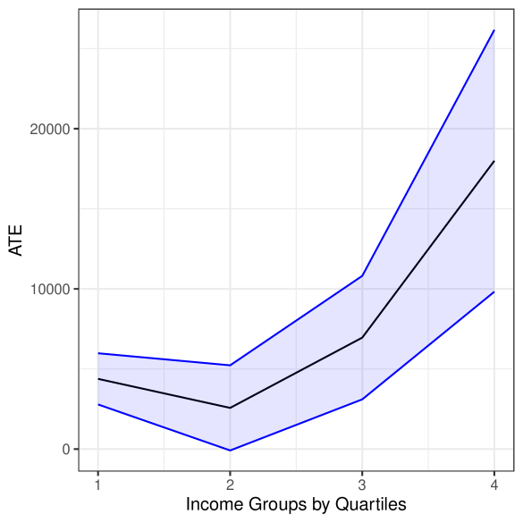
The first three columns of Table 1 shows the estimates for the average treatment effect (ATE) of 401(k) eligibility on net financial assets under this conditional ignorability assumption. For these estimates, we follow the same strategy used in Chernozhukov et al. (2018a), and we estimate the ATE using DML with Random Forests, considering both a partially linear model (PLM), and a nonparametric model (NPM). We use Random Forest both for the outcome and treatment regression and estimate the parameters using DML with 5-fold cross-fitting. In order to reduce the variance that stems from sample splitting, we repeat the procedure 5 times. Estimates are then combined using the median as the final estimate, incorporating variation across experiments into the standard error as described in Chernozhukov et al. (2018a). As we can see, after flexibly taking into account observed confounding factors, although the estimates of the effect of 401(k) eligibility on net financial assets are substantially attenuated, they are still large, positive and statistically significant (approximately $9,000 for the PLM and $8,000 for the NPM). With the nonparametric model, we further explore heterogeneous treatment effects, by analyzing the ATE within income quartile groups. The results are shown in Figure 3(a). We see that the ATE varies substantially across groups, with effects ranging from approximately $4,000 (first quartile) to almost $18,000 (last quartile).
<details>
<summary>x1.png Details</summary>
### Visual Description
## Line Chart: ATE by Income Groups by Quartiles
### Overview
The image is a line chart displaying the Average Treatment Effect (ATE) across different income groups, divided into quartiles. The chart shows a trend of ATE increasing with higher income quartiles, with a shaded area indicating the uncertainty or variability around the ATE estimates.
### Components/Axes
* **X-axis:** "Income Groups by Quartiles" with labels 1, 2, 3, and 4.
* **Y-axis:** "ATE" (Average Treatment Effect) with scale markers at 0, 10000, and 20000.
* **Data Series:** A single data series represented by a black line, with a blue shaded area around the line indicating a confidence interval or standard error. There is no explicit legend.
### Detailed Analysis
* **Income Group 1:** ATE is approximately 4000, with a range from approximately 2000 to 6000 (based on the shaded area).
* **Income Group 2:** ATE decreases to approximately 3000, with a range from approximately 0 to 6000.
* **Income Group 3:** ATE increases to approximately 8000, with a range from approximately 3000 to 11000.
* **Income Group 4:** ATE increases significantly to approximately 18000, with a range from approximately 10000 to 24000.
**Trend Verification:**
* The black line representing the ATE starts at approximately 4000 for Income Group 1.
* The line decreases to approximately 3000 for Income Group 2.
* The line then increases to approximately 8000 for Income Group 3.
* Finally, the line increases sharply to approximately 18000 for Income Group 4.
### Key Observations
* The ATE is lowest for the second income quartile.
* There is a substantial increase in ATE from the third to the fourth income quartile.
* The shaded area, representing uncertainty, widens as income increases, suggesting greater variability in ATE estimates for higher income groups.
### Interpretation
The chart suggests that the Average Treatment Effect is positively correlated with income, particularly in the higher income quartiles. The initial decrease from the first to the second quartile could indicate a non-linear relationship or the influence of other factors. The widening uncertainty range for higher income groups may reflect greater heterogeneity or smaller sample sizes within those groups. The data demonstrates a clear trend of increasing ATE as income increases, especially when moving from the third to the fourth income quartile.
</details>
(a) Estimates under no confounding.
<details>
<summary>x2.png Details</summary>
### Visual Description
## Line Chart: ATE vs. Income Groups by Quartiles
### Overview
The image is a line chart showing the relationship between Average Treatment Effect (ATE) and Income Groups by Quartiles. The chart displays a central tendency line (black) along with upper and lower bounds (red lines) and a shaded area (blue) representing the confidence interval. The x-axis represents income groups divided into quartiles (1 to 4), and the y-axis represents the ATE.
### Components/Axes
* **X-axis:** "Income Groups by Quartiles" with markers at 1, 2, 3, and 4.
* **Y-axis:** "ATE" with markers at 0, 10000, 20000, and 30000.
* **Data Series:**
* Black line: Represents the central tendency of ATE for each income quartile.
* Red lines: Represents the upper and lower bounds of ATE for each income quartile.
* Blue shaded area: Represents the confidence interval around the ATE.
### Detailed Analysis
* **Income Group 1:**
* Black line (ATE): Approximately 4000.
* Red line (Upper Bound): Approximately 7000.
* Red line (Lower Bound): Approximately 2000.
* Blue shaded area: Extends from approximately 7000 to 2000.
* **Income Group 2:**
* Black line (ATE): Approximately 3000.
* Red line (Upper Bound): Approximately 6000.
* Red line (Lower Bound): Approximately 500.
* Blue shaded area: Extends from approximately 6000 to 500.
* **Income Group 3:**
* Black line (ATE): Approximately 9000.
* Red line (Upper Bound): Approximately 13000.
* Red line (Lower Bound): Approximately 4000.
* Blue shaded area: Extends from approximately 13000 to 4000.
* **Income Group 4:**
* Black line (ATE): Approximately 18000.
* Red line (Upper Bound): Approximately 23000.
* Red line (Lower Bound): Approximately 11000.
* Blue shaded area: Extends from approximately 23000 to 11000.
### Key Observations
* The ATE generally increases as the income group quartile increases.
* The confidence interval (blue shaded area) widens as the income group quartile increases, indicating greater uncertainty in the ATE for higher income groups.
* The red lines representing the upper and lower bounds also diverge as the income group quartile increases.
### Interpretation
The chart suggests a positive correlation between income group quartile and Average Treatment Effect (ATE). As income increases, the ATE tends to increase as well. However, the widening confidence interval indicates that the effect of treatment may be more variable or less precisely estimated for higher income groups. This could be due to various factors, such as differences in treatment adherence, access to resources, or other confounding variables that are more prevalent or have a greater impact on higher income individuals. The initial dip in ATE from Income Group 1 to Income Group 2 could be due to a variety of factors and warrants further investigation.
</details>
(b) Bounds under posited confounding.
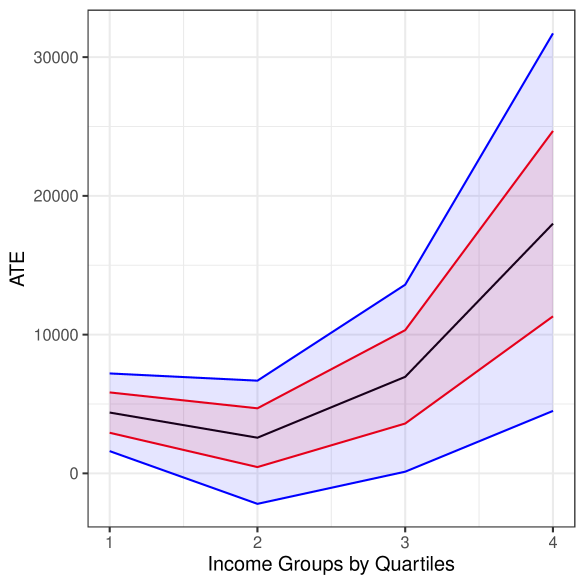
Figure 3. Estimate (black), bounds (red), and confidence bounds (blue) for the ATE by income quartiles. Confounding scenario: $\rho^{2}=1$ ; $C^{2}_{Y}≈ 0.04$ ; $C^{2}_{D}≈ 0.03$ . Significance level of $5\%$ .
5.2. Sensitivity analysis
It is now useful to consider scenarios in which conditional ignorability fails. Figure 2(b) presents one such scenario, where a violation of conditional ignorability is credible. We note that Figure 2(b) is just one example, and our sensitivity analysis results hold for any model in which conditional ignorability holds given observed variables and latent confounders. Employers often offer a benefit in which they “match” a proportion of an employee’s contribution to their 401(k) up to 5% of the employee’s salaries. The model in Figure 2(b) allows this “matched amount,” denoted by $M$ , to be determined by unobserved firm characteristics $A$ , observed worker characteristics $X$ , and by 401(k) eligibility $D$ . In this model, adjustment for $X$ alone is not sufficient for control of confounding. Instead, we now need to condition both on observed covariates $X$ and latent confounders $A$ for ignorability to hold. Note that in this case the average treatment effect is still defined as ${\mathrm{E}}[Y(1)-Y(0)]$ . The relevant counterfactuals $Y(d)$ are obtained by setting $D=d$ for all descendants of $D$ , that is $Y(d)=g_{Y}(d,M(d),X,\epsilon_{Y})$ , where $M(d)=g_{M}(d,F,X,\epsilon_{M}).$ How strong would the omitted firm characteristics $A$ have to be in order to overturn our previous conclusions? And how plausible are the strengths revealed to be problematic? In what follows, we use our sensitivity analysis results to address these questions.
5.2.1. Minimal sensitivity reporting.
In reporting empirical results, the following definition will be useful.
**Definition 2 (Robustness Values)**
*The robustness $\text{RV}_{\theta,a}$ stands for the minimum upper bound $RV$ on both sensitivity parameters, $R^{2}_{y-g_{s}\sim g-g_{s}}≤\text{RV}$ and $1-R^{2}_{\alpha\sim\alpha_{s}}≤\text{RV}$ , such that the confidence bound $[l,u]$ of Theorem 4 includes $\theta$ , at the significance level $a$ .*
Whereas standard errors, t-values or p-values communicate how robust the short estimate is to sampling errors, the idea of robustness values is to quickly communicate how robust the short estimate is to systematic errors due to residual confounding. For example, $\text{RV}_{\theta=0,a=.05}$ measures the minimal strength on both confounding factors such that the estimated confidence bound for the ATE would include zero, at the 5% significance level.
Table 1 illustrates our proposal for a minimal sensitivity reporting of causal effect estimates. Beyond the usual estimates under the assumption of conditional ignorability, it reports the robustness values of the short estimate. Starting with the PLM, the $\text{RV}_{\theta=0,a=0.05}=5.4\%$ means that unobserved confounders that explain less than 5.4% of the residual variation, both of the treatment, and of the outcome, are not sufficiently strong to bring the lower limit of the confidence bound to zero, at the 5% significance level. Moving to the nonparametric model, we obtain a similar, but somewhat lower value of $\text{RV}_{\theta=0,a=0.05}=4.5\%$ . The RV thus provides a quick and meaningful reference point that summarizes the robustness of the short estimate against unobserved confounding—any postulated confounding scenario that does not meet this minimal criterion of strength cannot overturn the results of the original study.
5.2.2. Main confounding scenario.
We now proceed to construct a particular confounding scenario, based on the contextual details of the problem. We start with the assumption that $A$ explains as much variation in net financial assets as the total variation of the maximal matched amount of income (5%) over the period of three years (roughly the period over which the effect is measured). This strategy is based on a suggestion by James Poterba. In the worst case scenario, this would lead to an additional $3\%$ of total variation explained, resulting in a partial $R^{2}$ of outcome with omitted firm characteristics $A$ of $C_{Y}^{2}=\eta^{2}_{Y\sim F|DX}=4\%$ . $\eta^{2}_{Y\sim F|DX}=\frac{\eta^{2}_{Y\sim FDX}-\eta^{2}_{Y\sim DX}}{1-\eta^{%
2}_{Y\sim DX}}=\frac{0.28+0.03-0.28}{1-0.28}≈ 4\%,$ This amounts to a relative increase of approximately 10% in the baseline $R^{2}$ of the outcome regression of 28%. Following similar reasoning, and more conservatively, we posit that omitted firm characteristics can explain an additional $2.5\%$ of the variation in 401(k) eligibility, corresponding to a $22\%$ relative increase in the baseline $R^{2}$ of the treatment regression of 11.4%. For the partially linear model, this results in $1-R^{2}_{\alpha\sim\alpha_{s}}=\eta^{2}_{D\sim F\mid X}≈ 3\%$ (and also $C^{2}_{D}≈ 3\%$ ). $1-R^{2}_{\alpha\sim\alpha_{s}}=\eta^{2}_{D\sim F|X}=\frac{\eta^{2}_{D\sim FX}-%
\eta^{2}_{D\sim X}}{1-\eta^{2}_{D\sim X}}=\frac{0.114+.025-0.114}{1-0.114}%
≈ 3\%.$ We adopt the same scenario for the nonparametric model, with the understanding that now this would correspond to gains in precision (see Remark 2). Since both $\eta^{2}_{Y\sim F|DX}≈ 4\%$ and $1-R^{2}_{\alpha\sim\alpha_{s}}≈ 3\%$ are below the robustness value of 5.4% (or 4.5%), we immediately conclude that such confounding scenario is not capable of bringing the lower limit of the confidence bound of the ATE to zero.
Table 2. Estimate, bias, and bounds for the ATE. Significance level of 5%. Standard errors in parenthesis. Confounding scenario: $\rho^{2}=1$ ; $C^{2}_{Y}≈ 0.04$ ; $C^{2}_{D}≈ 0.03$ .
The exact bias, bounds, and confidence bounds on the ATE implied by the posited scenario are shown in Table 2. We use the same estimation procedure as described in footnote 10. Starting with the partially linear model, the confounding scenario has an estimated absolute value of the bias of $\$4,196$ . Accounting for statistical uncertainty, we obtain a lower limit for the confidence bound of $\$2,497$ . The results for the nonparametric model are qualitatively similar, with a bias of similar magnitude, and point estimates, bounds, and confidence bounds for the ATE shifted down by roughly one thousand dollars. Confidence bounds for group-wise ATEs can also be computed, and are shown in Figure 3(b). Note how the bounds are still largely positive, with only a small excursion into the negative side in the case of the second quartile group. These results suggest that the main qualitative findings reported in earlier studies are relatively robust to plausible violations of unconfoundedness, such as the one specified by our confounding scenario.
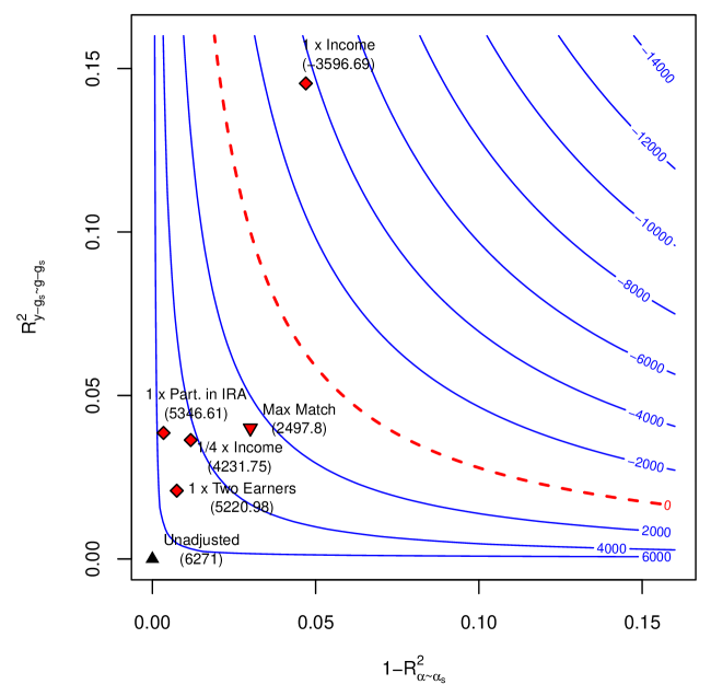
5.2.3. Sensitivity contour plots and benchmarks
A useful tool for visualizing the whole sensitivity range of the target parameter, under different assumptions regarding the strength of confounding, is a bivariate contour plot showing the collection of curves in the space of $R^{2}$ values along which the confidence bounds are constant (Imbens, 2003; Cinelli and Hazlett, 2020). These plots allow investigators to quickly and easily assess the robustness of their findings against any postulated confounding scenario. Here we focus on contour plots for the lower limit of the confidence bounds, as this is the direction of the bias that threatens the preferred hypothesis in this empirical example. Analogous contours can be constructed for the upper limit of the confidence bounds, and are omitted.
<details>
<summary>x3.png Details</summary>
### Visual Description
## Contour Plot: R-squared Values
### Overview
The image is a contour plot showing the relationship between two R-squared values (R²y~gs~g-gs and 1-R²α~αs) and their impact on a third, implied variable represented by the blue contour lines. Several scenarios are plotted as points on the graph, each labeled with a description and a numerical value. A red dashed line separates regions of positive and negative values.
### Components/Axes
* **X-axis:** 1-R²α~αs, ranging from 0.00 to 0.15 in increments of 0.05.
* **Y-axis:** R²y~gs~g-gs, ranging from 0.00 to 0.15 in increments of 0.05.
* **Contour Lines (Blue):** Represent constant values of the implied variable, labeled with values ranging from -14000 to 6000. The contour lines are denser towards the top-left corner of the plot.
* **Red Dashed Line:** Separates the regions of positive and negative values of the implied variable.
* **Data Points:** Represent different scenarios, each marked with a symbol and a label.
### Detailed Analysis
**Data Points:**
* **Unadjusted (Black Triangle):** Located at approximately (0.00, 0.00), value (6271).
* **1 x Two Earners (Red Diamond):** Located at approximately (0.01, 0.02), value (5220.98).
* **1/4 x Income (Red Diamond):** Located at approximately (0.02, 0.03), value (4231.75).
* **1 x Part. in IRA (Red Diamond):** Located at approximately (0.00, 0.04), value (5346.61).
* **Max Match (Red Triangle):** Located at approximately (0.04, 0.04), value (2497.8).
* **1 x Income (Red Diamond):** Located at approximately (0.04, 0.15), value (-3596.69).
**Contour Lines:**
* The blue contour lines represent values of the implied variable. From the top right to the bottom left, the values are approximately: -14000, -12000, -10000, -8000, -6000, -4000, -2000, 0, 2000, 4000, 6000.
* The contour lines are closer together in the top-left, indicating a steeper gradient in that region.
**Red Dashed Line:**
* The red dashed line separates the positive and negative regions of the implied variable. It starts near (0.00, 0.15) and curves towards (0.15, 0.00).
### Key Observations
* The "1 x Income" scenario has a negative value for the implied variable, while the other scenarios have positive values.
* The "Unadjusted" scenario has the highest positive value for the implied variable among the plotted scenarios.
* The contour lines suggest that the implied variable is highly sensitive to changes in both R-squared values in the top-left region of the plot.
### Interpretation
The contour plot visualizes the relationship between two R-squared values and their combined effect on an implied variable. The different scenarios represent various conditions or strategies, and their positions on the plot indicate their impact on the implied variable. The contour lines provide a sense of how the implied variable changes as the R-squared values vary. The red dashed line is a critical boundary, separating scenarios that result in positive or negative outcomes for the implied variable. The density of the contour lines indicates the sensitivity of the implied variable to changes in the R-squared values. The plot allows for a comparison of different scenarios and an understanding of how they affect the implied variable.
</details>
(a) Lower limit confidence bound ( $|\rho|=1)$ .
<details>
<summary>x4.png Details</summary>
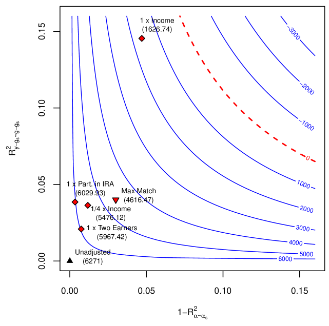
### Visual Description
## Contour Plot: R-squared Relationship
### Overview
The image is a contour plot showing the relationship between two R-squared values: R²y-gs-g-gs on the y-axis and 1-R²α-αs on the x-axis. The plot includes blue contour lines representing different values, a red dashed line, and several data points marked with symbols and labels.
### Components/Axes
* **X-axis:** 1-R²α-αs, ranging from 0.00 to 0.15 in increments of 0.05.
* **Y-axis:** R²y-gs-g-gs, ranging from 0.00 to 0.15 in increments of 0.05.
* **Contour Lines:** Blue lines representing constant values, labeled with values from -3000 to 6000.
* **Red Dashed Line:** A dashed red line that separates regions of the plot.
* **Data Points:** Several data points are plotted, each labeled with a description and a numerical value in parentheses.
### Detailed Analysis
**Data Points:**
* **Unadjusted:** Located at approximately (0.00, 0.00), marked with a black triangle, value (6271).
* **1 x Two Earners:** Located at approximately (0.00, 0.02), marked with a red diamond, value (5967.42).
* **1/4 x Income:** Located at approximately (0.01, 0.03), marked with a red diamond, value (5476.12).
* **1 x Part. in IRA:** Located at approximately (0.00, 0.05), marked with a red diamond, value (6029.93).
* **Max Match:** Located at approximately (0.04, 0.04), marked with a red inverted triangle, value (4616.47).
* **1 x Income:** Located at approximately (0.03, 0.15), marked with a red diamond, value (1626.74).
**Contour Lines:**
* The blue contour lines represent values ranging from -3000 to 6000. The lines are denser in the bottom-left corner, indicating a steeper gradient in that region.
* The contour lines generally curve upwards and to the right.
* Specific contour line values: -3000, -2000, -1000, -0, 1000, 2000, 3000, 4000, 5000, 6000.
**Red Dashed Line:**
* The red dashed line starts at approximately (0.08, 0.00) and curves upwards and to the right, separating the plot into two regions.
### Key Observations
* The "Unadjusted" data point is located at the origin (0,0).
* The "1 x Income" data point has the lowest value (1626.74) and is located in the upper-left region of the plot.
* The contour lines indicate a complex relationship between the two R-squared values.
### Interpretation
The contour plot visualizes the relationship between two R-squared values, likely representing the variance explained by different models or factors. The data points represent specific scenarios or conditions, with the numerical values in parentheses potentially indicating a metric associated with each scenario (e.g., cost, benefit, or a specific outcome).
The contour lines show how the value changes as the two R-squared values vary. The red dashed line might represent a threshold or boundary of interest.
The placement of the data points relative to the contour lines and the red dashed line provides insights into the performance or characteristics of each scenario. For example, the "1 x Income" scenario has a low value and is located in a region with lower contour values, suggesting it might be associated with less desirable outcomes compared to other scenarios.
</details>
(b) Lower limit confidence bound ( $|\rho|=1/2)$ .
Figure 4. Sensitivity contour plots 401(k), PLM. Significance level $a=0.05$ .
Starting with the partially linear model, the results are shown in Figure 4(a). The horizontal axis describes the fraction of residual variation of the treatment explained by unobserved confounders, whereas the vertical axis describes the share of residual variation of the outcome explained by unobserved confounders. The contour lines show the lower limit of the confidence bounds $[l,u]$ for the ATE (see Theorem 4), given a pair of hypothesized values of partial $R^{2}$ . Note $\text{RV}_{\theta=0,a=0.05}$ of Table 1 is simply the point where the 45-degree line crosses the contour line of zero (red dashed line), offering a convenient summary of the critical contour. We can further place reference points on the contour plots, indicating plausible bounds on the strength of confounding, under alternative assumptions about the maximum explanatory power of omitted variables. The red triangle point on the plot— Max Match —shows the bounds on the partial $R^{2}$ as previously discussed, resulting in a lower limit of the confidence bound for the ATE of $2,497, in accordance with Table 2. Note here the correlation $|\rho|$ is set to its upper bound of 1.
Another approach to construct confounding scenarios is to use observed covariates to bound the plausible strength of unobserved covariates. For instance, in our empirical example, we know that employment decisions are largely driven by salary considerations. Similarly, salary is clearly an important determinant of net financial assets. One could therefore argue that it is implausible to imagine other latent firm characteristics that would be even a fraction as strong as the observed income of individuals, in terms of explanatory power in predicting 401(k) eligibility and net financial assets. Whenever such claims of relative importance can be made, they can be used to set plausible bounds on the strength of unmeasured confounding. Formal details of this benchmarking procedure are provided in Section F of the Appendix.
The red diamonds of Figure 4(a) shows the bounds on the strength of the latent variable $A$ if it were as strong as (i) income (1 x Income), (ii) whether a worker has an individual retirement account (1 x Part. in IRA), and (iii) whether the worker’s family has a two-earner status (1 x Two Earners). Note that, apart from income, latent variables as strong as these covariates would result in a weaker confounding scenario than the one we have previously considered (Max Match). As for income, the worst-case bound indicates that omitted firm characteristics as important as income would indeed be sufficient to overturn the original results. However, one could argue such scenario to be implausible, as it is hard to imagine latent firm characteristics that would explain more variation in job choice than income itself. A more realistic, but still conservative, scenario is thus provided by the benchmark point 1/4 x Income, which shows the bound on the strength of $A$ if it were 25% as strong as income in predicting treatment and outcome variation. Note this scenario is comparable to the Max Match scenario, and not enough to bring the lower limit of the confidence bound to zero.
<details>
<summary>x5.png Details</summary>
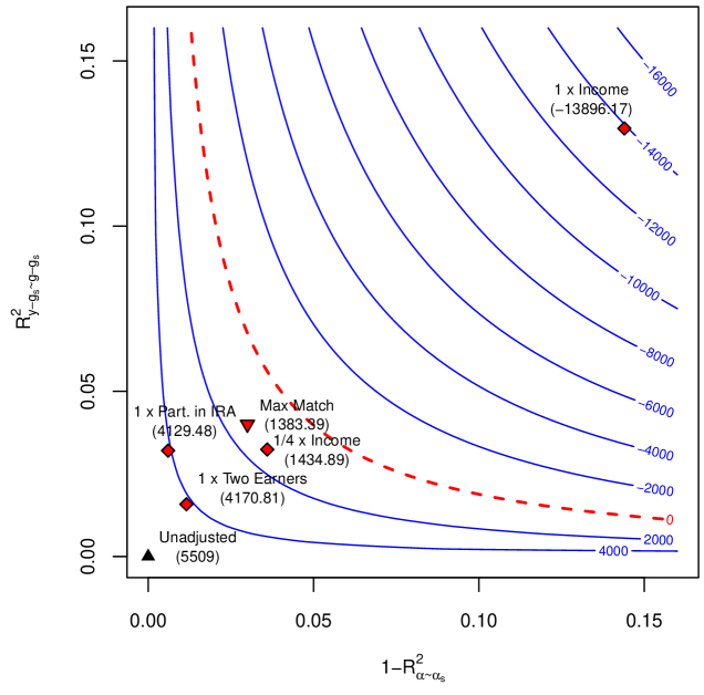
### Visual Description
## Contour Plot: R-squared Tradeoffs
### Overview
The image is a contour plot illustrating the trade-off between two R-squared values: `R²y-gs~g-gs` on the y-axis and `1-R²α~αs` on the x-axis. The blue contour lines represent different levels of a third, unstated variable. Several data points, labeled with descriptions and numerical values, are plotted on the graph. A dashed red line highlights a specific region of interest.
### Components/Axes
* **X-axis:** `1-R²α~αs`. Scale ranges from 0.00 to 0.15 in increments of 0.05.
* **Y-axis:** `R²y-gs~g-gs`. Scale ranges from 0.00 to 0.15 in increments of 0.05.
* **Contour Lines:** Blue lines representing constant values. The values are labeled in blue text and range from -16000 to 4000.
* **Data Points:** Several data points are plotted, each labeled with a description and a numerical value in parentheses.
* **Red Dashed Line:** A curve separating different regions of the plot.
### Detailed Analysis
**Data Points:**
* **Unadjusted:** Located at approximately (0.00, 0.00), marked with a black triangle. Value: (5509)
* **1 x Part. in IRA:** Located at approximately (0.00, 0.04), marked with a red diamond. Value: (4129.48)
* **1 x Two Earners:** Located at approximately (0.02, 0.02), marked with a red diamond. Value: (4170.81)
* **1/4 x Income:** Located at approximately (0.04, 0.03), marked with a red diamond. Value: (1434.89)
* **Max Match:** Located at approximately (0.04, 0.05), marked with a red inverted triangle. Value: (1383.39)
* **1 x Income:** Located at approximately (0.15, 0.14), marked with a red diamond. Value: (-13896.17)
**Contour Lines:**
The blue contour lines are labeled with the following values:
* 4000
* 2000
* 0
* -2000
* -4000
* -6000
* -8000
* -10000
* -12000
* -14000
* -16000
The contour lines generally curve upwards and to the right.
**Red Dashed Line:**
The red dashed line starts near (0.00, 0.00) and curves upwards and to the right, passing between the "Max Match" and "1/4 x Income" data points.
### Key Observations
* The "Unadjusted" data point has the lowest values on both axes.
* The "1 x Income" data point has the highest values on both axes, and a significantly negative contour value.
* The contour lines indicate a trade-off between the two R-squared values. Increasing one generally requires decreasing the other to stay on the same contour line.
* The red dashed line separates the data points into two groups.
### Interpretation
The plot visualizes the relationship between two R-squared metrics, likely representing the explanatory power of different models or scenarios. The contour lines represent a third, unstated variable, which could be a cost function or a utility measure. The data points represent specific scenarios or models, with their positions indicating their performance in terms of the two R-squared metrics.
The red dashed line likely represents a constraint or a threshold. Data points above and to the left of the line might be considered more desirable, depending on the context. The "1 x Income" scenario appears to be an outlier, with a very high value on the x-axis and a very low (negative) contour value. This suggests that while it might explain a lot of the variance in one variable (represented by the x-axis), it performs poorly in terms of the unstated variable represented by the contour lines.
</details>
(a) Lower limit confidence bound ( $|\rho|=1)$ .
<details>
<summary>x6.png Details</summary>
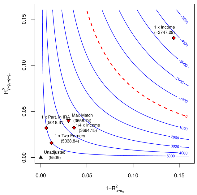
### Visual Description
## Contour Plot: R-squared Values
### Overview
The image is a contour plot showing the relationship between two R-squared values, labeled as `R²y-gs~g-gs` on the y-axis and `1-R²α~αs` on the x-axis. The plot displays several blue contour lines representing different constant values, ranging from -5000 to 5000. A dashed red line is also present. Several data points, represented by red diamonds and a black triangle, are plotted on the graph, each labeled with a description and a numerical value.
### Components/Axes
* **X-axis:** `1-R²α~αs`, ranging from 0.00 to 0.15 in increments of 0.05.
* **Y-axis:** `R²y-gs~g-gs`, ranging from 0.00 to 0.15 in increments of 0.05.
* **Contour Lines:** Blue lines representing constant values. The values are labeled along the lines and range from -5000 to 5000.
* **Dashed Line:** A red dashed line that appears to separate regions of the plot.
* **Data Points:**
* Red diamonds:
* "1 x Part. in IRA (5018.31)" located at approximately (0.01, 0.03).
* "1/4 x Income (3684.15)" located at approximately (0.05, 0.03).
* "1 x Two Earners (5038.84)" located at approximately (0.02, 0.02).
* "1 x Income (-3747.29)" located at approximately (0.15, 0.14).
* Red triangle:
* "Max Match (3658.74)" located at approximately (0.04, 0.04).
* Black triangle:
* "Unadjusted (5509)" located at approximately (0.00, 0.00).
### Detailed Analysis
* **Contour Lines:** The blue contour lines are curved, generally increasing in value as they move towards the bottom-right corner of the plot.
* **Dashed Red Line:** The dashed red line starts near the top-left and curves towards the bottom-right.
* **Data Point Locations:**
* "Unadjusted (5509)" is located at the origin (0.00, 0.00).
* "1 x Two Earners (5038.84)" is located near the origin, slightly above and to the right.
* "1 x Part. in IRA (5018.31)" is located above "1 x Two Earners (5038.84)".
* "Max Match (3658.74)" is located to the right and slightly above "1 x Part. in IRA (5018.31)".
* "1/4 x Income (3684.15)" is located close to "Max Match (3658.74)".
* "1 x Income (-3747.29)" is located in the top-right corner of the plot.
### Key Observations
* The contour lines indicate a complex relationship between the two R-squared values.
* The data points are clustered in the lower-left corner, except for "1 x Income (-3747.29)", which is located in the top-right corner.
* The "Unadjusted (5509)" data point is at the origin.
### Interpretation
The contour plot visualizes how different factors (e.g., participation in IRA, income levels, two earners) affect the relationship between two R-squared values. The contour lines represent constant values, allowing for the comparison of different scenarios. The data points indicate the specific R-squared values for each scenario. The clustering of data points in the lower-left corner suggests that these scenarios have similar effects on the R-squared values. The "1 x Income (-3747.29)" data point, located in the top-right corner, represents an outlier, indicating a significantly different effect on the R-squared values compared to the other scenarios. The red dashed line might represent a threshold or boundary, separating regions with different characteristics or implications.
</details>
(b) Lower limit confidence bound ( $|\rho|=1/2)$ .
Figure 5. Sensitivity contour plots 401(k), NPM. Significance level $a=0.05$ .
All results of Figure 4(a) were computed under the very conservative assumption that, given a pair of partial $R^{2}$ values for the latent variable $A$ , the confounders enter both the outcome and treatment equations in a way that maximizes the bias, resulting in $|\rho|=1$ . Although we can always construct such a confounder (absent further assumptions on the data generating process), it may be an unnatural scenario in practice, especially in nonlinear models. For an extreme example, consider the model $D=A^{2}$ , $Y=\theta D+A$ , with $A\sim N(0,1)$ . Even though the latent variable $A$ nonparametrically explains 100% of the residual variation in both the treatment and the outcome equations, the nonlinearity of the confounding model attenuates this bias, making it effectively zero ( $A^{2}$ is uncorrelated with $A$ ). Thus, similar benchmarking procedures used for assessing the plausibility of the $R^{2}$ values can also be employed to calibrate judgments on the magnitude of $\rho$ . Section F of the appendix shows that in fact none of the observed covariates result in $|\rho|$ values exceeding 1/2. With this in mind, Figure 4(b) presents the same contour plots as before, but now with $|\rho|$ set to a less conservative value of 1/2. Note how this substantially attenuates the bias, with the lower limits of the confidence bounds reaching approximately $\$4,600$ and $\$5,400$ for the Max Match and 1/4 x Income, respectively.
Sensitivity contour plots for the nonparametric model are similar but slightly more conservative, and are provided in Figure 5. The interpretation of the contours is the same as before, with the main difference being that the horizontal axis now describes gains in precision instead of gains in variance explained (see, e.g, Remark 2).
6. Conclusion
In this paper we provide a general theory of omitted variable bias for continuous linear functionals of the conditional expectation function of the outcome—all for general, nonparametric, causal models, while naturally allowing for (semi-)parametric restrictions (such as partial linearity), when such assumptions are made. We allow for arbitrary (e.g., binary or continuous) treatment and outcome variables, and we show that the bounds on the bias depends only on the maximum explanatory power of latent variables. We provide theoretical details of many leading causal estimands, and, in particular, we derive novel bounds for the important special cases of average treatment effects in partially linear models, in nonparametric models with a binary treatment, as well as for average causal derivatives. Finally, we leverage the Riesz representation of our bounds to offer flexible statistical inference through (debiased) machine learning, with rigorous coverage guarantees. Therefore, we provide a concise and complete solution to the OVB problem and the bounding of its size, as well performing statistical inference on these bounds, for a rich and important class of causal parameters.
Our results can potentially be extended to nonlinear functionals, such as those arising in instrumental variable (IV) methods. For instance, consider a variant of the IV problem (Imbens and Angrist, 1994), where the instrumental variable $Z$ is valid only when conditioning both on observed covariates $X$ , and latent variables $A$ . In this case, the IV estimand is given by the ratio of two average treatment effects,
$$
\mathrm{IV}=\frac{\text{ATE}(Z\to Y)}{\text{ATE}(Z\to D)}.
$$
Both the numerator and denominator can be bounded using the methods for the ATE proposed in this paper. Another interesting direction for future work is to consider causal estimands that are functionals of the long quantile regression, or causal estimands that are values of a policy in dynamic stochastic programming. When the degree of confounding is small, it seems possible to use the results in Chernozhukov et al. (2022a) to derive approximate bounds on the bias that can be estimated using debiased ML approaches.
Data Availability, Conflict of Interests, and Funding
Data availability.
All data is is publicly available in our GitHub repository: https://github.com/carloscinelli/dml.sensemakr.
Conflict of interest.
There are no relevant financial or nonfinancial competing interests to report.
Funding.
This research was partially funded by the Royalty Research Fund at the University of Washington.
References
- Altonji et al. (2005) Joseph G Altonji, Todd E Elder, and Christopher R Taber. Selection on observed and unobserved variables: Assessing the effectiveness of catholic schools. Journal of political economy, 113(1):151–184, 2005.
- Angrist and Pischke (2009) Joshua D. Angrist and Jorn-Steffan Pischke. Mostly Harmless Econometrics: An Empiricist’s Companion. Princeton University Press, 2009.
- Aronow and Samii (2016) Peter M Aronow and Cyrus Samii. Does regression produce representative estimates of causal effects? American Journal of Political Science, 60(1):250–267, 2016.
- Athey et al. (2019) Susan Athey, Julie Tibshirani, and Stefan Wager. Generalized random forests. The Annals of Statistics, 47(2):1148–1178, 2019.
- Belloni et al. (2013) A. Belloni, V. Chernozhukov, I. Fernández-Val, and C. Hansen. Program Evaluation with High-Dimensional Data. ArXiv e-prints, November 2013.
- Bickel et al. (1993) Peter J Bickel, Chris AJ Klaassen, Ya’acov Ritov, and Jon A Wellner. Efficient and Adaptive Estimation for Semiparametric Models, volume 4. Johns Hopkins University Press, 1993.
- Blackwell (2013) Matthew Blackwell. A selection bias approach to sensitivity analysis for causal effects. Political Analysis, 22(2):169–182, 2013.
- Blundell et al. (2012) Richard Blundell, Joel L Horowitz, and Matthias Parey. Measuring the price responsiveness of gasoline demand: Economic shape restrictions and nonparametric demand estimation. Quantitative Economics, 3(1):29–51, 2012.
- Blundell et al. (2017) Richard Blundell, Joel Horowitz, and Matthias Parey. Nonparametric estimation of a nonseparable demand function under the slutsky inequality restriction. Review of Economics and Statistics, 99(2):291–304, 2017.
- Bonvini and Kennedy (2021) Matteo Bonvini and Edward H Kennedy. Sensitivity analysis via the proportion of unmeasured confounding. Journal of the American Statistical Association, pages 1–11, 2021.
- Brumback et al. (2004) Babette A Brumback, Miguel A Hernán, Sebastien JPA Haneuse, and James M Robins. Sensitivity analyses for unmeasured confounding assuming a marginal structural model for repeated measures. Statistics in medicine, 23(5):749–767, 2004.
- Chernozhukov et al. (2018a) Victor Chernozhukov, Denis Chetverikov, Mert Demirer, Esther Duflo, Christian Hansen, Whitney Newey, and James Robins. Double/debiased machine learning for treatment and structural parameters. The Econometrics Journal, 2018a. ArXiv 2016; arXiv:1608.00060.
- Chernozhukov et al. (2018b) Victor Chernozhukov, Whitney Newey, and Rahul Singh. De-biased machine learning of global and local parameters using regularized riesz representers. arXiv preprint arXiv:1802.08667, 2018b.
- Chernozhukov et al. (2020) Victor Chernozhukov, Whitney Newey, Rahul Singh, and Vasilis Syrgkanis. Adversarial estimation of riesz representers. arXiv preprint arXiv:2101.00009, 2020.
- Chernozhukov et al. (2021) Victor Chernozhukov, Whitney K Newey, Victor Quintas-Martinez, and Vasilis Syrgkanis. Automatic debiased machine learning via neural nets for generalized linear regression. arXiv preprint arXiv:2104.14737, 2021.
- Chernozhukov et al. (2022a) Victor Chernozhukov, Juan Carlos Escanciano, Hidehiko Ichimura, Whitney K Newey, and James M Robins. Locally robust semiparametric estimation. Econometrica, 2022a.
- Chernozhukov et al. (2022b) Victor Chernozhukov, Whitney K. Newey, Victor Quintas-Martinez, and Vasilis Syrgkanis. Riesznet and forestriesz: Automatic debiased machine learning with neural nets and random forests. International Conference on Machine Learning, 2022b.
- Chernozhukov et al. (2022c) Victor Chernozhukov, Whitney K Newey, and Rahul Singh. Automatic debiased machine learning of causal and structural effects. Econometrica, 2022c.
- Chetverikov and Wilhelm (2017) Denis Chetverikov and Daniel Wilhelm. Nonparametric instrumental variable estimation under monotonicity. Econometrica, 85(4):1303–1320, 2017. doi: https://doi.org/10.3982/ECTA13639.
- Chetverikov et al. (2018) Denis Chetverikov, Dongwoo Kim, and Daniel Wilhelm. Nonparametric instrumental-variable estimation. The Stata Journal, 18(4):937–950, 2018.
- Cinelli and Hazlett (2020) Carlos Cinelli and Chad Hazlett. Making sense of sensitivity: Extending omitted variable bias. Journal of the Royal Statistical Society: Series B (Statistical Methodology), 82(1):39–67, 2020.
- Cinelli et al. (2019) Carlos Cinelli, Daniel Kumor, Bryant Chen, Judea Pearl, and Elias Bareinboim. Sensitivity analysis of linear structural causal models. International Conference on Machine Learning, 2019.
- Detommaso et al. (2021) Gianluca Detommaso, Michael Brückner, Philip Schulz, and Victor Chernozhukov. Causal bias quantification for continuous treatment, 2021.
- Ding and VanderWeele (2016) Peng Ding and Tyler J VanderWeele. Sensitivity analysis without assumptions. Epidemiology (Cambridge, Mass.), 27(3):368, 2016.
- Doksum and Samarov (1995) Kjell Doksum and Alexander Samarov. Nonparametric estimation of global functionals and a measure of the explanatory power of covariates in regression. The Annals of Statistics, pages 1443–1473, 1995.
- Dorie et al. (2016) Vincent Dorie, Masataka Harada, Nicole Bohme Carnegie, and Jennifer Hill. A flexible, interpretable framework for assessing sensitivity to unmeasured confounding. Statistics in medicine, 35(20):3453–3470, 2016.
- Frank (2000) Kenneth A Frank. Impact of a confounding variable on a regression coefficient. Sociological Methods & Research, 29(2):147–194, 2000.
- Franks et al. (2020) AlexanderM Franks, Alexander D’Amour, and Avi Feller. Flexible sensitivity analysis for observational studies without observable implications. Journal of the American Statistical Association, 115(532):1730–1746, 2020.
- Goldberger (1991) Arthur Stanley Goldberger. A course in econometrics. Harvard University Press, 1991.
- Hasminskii and Ibragimov (1978) Rafail Z Hasminskii and Ildar A Ibragimov. On the nonparametric estimation of functionals. In Proceedings of the 2nd Prague Symposium on Asymptotic Statistics, pages 41–51, 1978.
- Imbens (2003) Guido W Imbens. Sensitivity to exogeneity assumptions in program evaluation. American Economic Review, 93(2):126–132, 2003.
- Imbens and Angrist (1994) Guido W. Imbens and Joshua D. Angrist. Identification and estimation of local average treatment effects. Econometrica, 62:467–475, 1994.
- Imbens and Rubin (2015) Guido W Imbens and Donald B Rubin. Causal inference in statistics, social, and biomedical sciences. Cambridge University Press, 2015.
- Jesson et al. (2021) Andrew Jesson, Sören Mindermann, Yarin Gal, and Uri Shalit. Quantifying ignorance in individual-level causal-effect estimates under hidden confounding. arXiv preprint arXiv:2103.04850, 2021.
- Kallus and Zhou (2018) Nathan Kallus and Angela Zhou. Confounding-robust policy improvement. arXiv preprint arXiv:1805.08593, 2018.
- Kallus et al. (2019) Nathan Kallus, Xiaojie Mao, and Angela Zhou. Interval estimation of individual-level causal effects under unobserved confounding. In The 22nd international conference on artificial intelligence and statistics, pages 2281–2290. PMLR, 2019.
- Levit (1975) Boris Ya Levit. On efficiency of a class of non-parametric estimates. Teoriya Veroyatnostei i ee Primeneniya, 20(4):738–754, 1975.
- Liu et al. (2013) Weiwei Liu, S Janet Kuramoto, and Elizabeth A Stuart. An introduction to sensitivity analysis for unobserved confounding in nonexperimental prevention research. Prevention science, 14(6):570–580, 2013.
- Masten and Poirier (2018) Matthew A Masten and Alexandre Poirier. Identification of treatment effects under conditional partial independence. Econometrica, 86(1):317–351, 2018.
- Newey (1994) Whitney K Newey. The asymptotic variance of semiparametric estimators. Econometrica: Journal of the Econometric Society, pages 1349–1382, 1994.
- ORNL (2004) Oak Ridge National Laboratory ORNL. 2001 national household travel survey: User guide. ORNL, 2004. URL http://nhts.ornl.gov/.
- Oster (2017) Emily Oster. Unobservable selection and coefficient stability: Theory and evidence. Journal of Business & Economic Statistics, pages 1–18, 2017.
- Oster (2019) Emily Oster. Unobservable selection and coefficient stability: Theory and evidence. Journal of Business & Economic Statistics, 37(2):187–204, 2019.
- Pearl (2009) Judea Pearl. Causality. Cambridge university press, 2009.
- Pearson (1905) Karl Pearson. On the general theory of skew correlation and non-linear regression. Dulau and Company, 1905.
- Pfanzagl and Wefelmeyer (1985) J Pfanzagl and W Wefelmeyer. Contributions to a general asymptotic statistical theory. Statistics & Risk Modeling, 3(3-4):379–388, 1985.
- Poterba et al. (1994) James M. Poterba, Steven F. Venti, and David A. Wise. 401(k) plans and tax-deferred savings. In D. A. Wise, editor, Studies in the Economics of Aging. Chicago, IL: University of Chicago Press, 1994.
- Poterba et al. (1995) James M. Poterba, Steven F. Venti, and David A. Wise. Do 401(k) contributions crowd out other personal saving? Journal of Public Economics, 58:1–32, 1995.
- Richardson et al. (2014) Amy Richardson, Michael G Hudgens, Peter B Gilbert, and Jason P Fine. Nonparametric bounds and sensitivity analysis of treatment effects. Statistical Science, 29(4):596, 2014.
- Robins (1999) James M Robins. Association, causation, and marginal structural models. Synthese, 121(1):151–179, 1999.
- Rosenbaum (1987) Paul R Rosenbaum. Sensitivity analysis for certain permutation inferences in matched observational studies. Biometrika, 74(1):13–26, 1987.
- Rosenbaum (2002) Paul R Rosenbaum. Observational studies. In Observational studies, pages 1–17. Springer, 2002.
- Rosenbaum and Rubin (1983a) Paul R Rosenbaum and Donald B Rubin. The central role of the propensity score in observational studies for causal effects. Biometrika, 70(1):41–55, 1983a.
- Rosenbaum and Rubin (1983b) Paul R Rosenbaum and Donald B Rubin. Assessing sensitivity to an unobserved binary covariate in an observational study with binary outcome. Journal of the Royal Statistical Society. Series B (Methodological), pages 212–218, 1983b.
- Scharfstein et al. (2021) Daniel O Scharfstein, Razieh Nabi, Edward H Kennedy, Ming-Yueh Huang, Matteo Bonvini, and Marcela Smid. Semiparametric sensitivity analysis: Unmeasured confounding in observational studies. arXiv preprint arXiv:2104.08300, 2021.
- Semenova and Chernozhukov (2021) Vira Semenova and Victor Chernozhukov. Debiased machine learning of conditional average treatment effects and other causal functions. The Econometrics Journal, 24(2):264–289, 2021.
- Słoczyński (2022) Tymon Słoczyński. Interpreting ols estimands when treatment effects are heterogeneous: smaller groups get larger weights. Review of Economics and Statistics, 104(3):501–509, 2022.
- Stoye (2009) Jörg Stoye. More on confidence intervals for partially identified parameters. Econometrica, 77(4):1299–1315, 2009.
- Tan (2006) Zhiqiang Tan. A distributional approach for causal inference using propensity scores. Journal of the American Statistical Association, 101(476):1619–1637, 2006.
- Van der Laan and Rose (2011) Mark J Van der Laan and Sherri Rose. Targeted learning: causal inference for observational and experimental data. Springer Science & Business Media, 2011.
- van der Vaart and Wellner (1996) A. W. van der Vaart and J. A. Wellner. Weak Convergence and Empirical Processes. Springer Series in Statistics, 1996.
- Vanderweele and Arah (2011) Tyler J. Vanderweele and Onyebuchi A. Arah. Bias formulas for sensitivity analysis of unmeasured confounding for general outcomes, treatments, and confounders. Epidemiology (Cambridge, Mass.), 22(1):42–52, January 2011.
- VanderWeele and Ding (2017) Tyler J VanderWeele and Peng Ding. Sensitivity analysis in observational research: introducing the E-value. Annals of Internal Medicine, 167(4):268–274, 2017.
- Veitch and Zaveri (2020) Victor Veitch and Anisha Zaveri. Sense and sensitivity analysis: Simple post-hoc analysis of bias due to unobserved confounding. Advances in Neural Information Processing Systems, 33:10999–11009, 2020.
- Wooldridge (2010) Jeffrey M. Wooldridge. Econometric Analysis of Cross Section and Panel Data. Cambridge, Massachusetts: The MIT Press, second edition, 2010.
- Yadlowsky et al. (2018) Steve Yadlowsky, Hongseok Namkoong, Sanjay Basu, John Duchi, and Lu Tian. Bounds on the conditional and average treatment effect with unobserved confounding factors. arXiv preprint arXiv:1808.09521, 2018.
- Zhao et al. (2019) Qingyuan Zhao, Dylan S Small, and Bhaswar B Bhattacharya. Sensitivity analysis for inverse probability weighting estimators via the percentile bootstrap. Journal of the Royal Statistical Society: Series B, 81(4):735–761, 2019.
Appendix A Preliminaries
A.1. Few Preliminaries
To prove supporting lemmas we recall the following standard definitions and results. Given two normed vector spaces $V$ and $W$ over the field of real numbers $\mathbb{R}$ , a linear map $A:V→ W$ is continuous if and only if it has a bounded operator norm:
$$
\displaystyle\|A\|_{op}:=\inf\{c\geq 0:\|Av\|\leq c\|v\|{\mbox{ for all }}v\in
V%
\}<\infty,
$$
where $\|·\|_{op}$ is the operator norm. The operator norm depends on the choice of norms for the normed vector spaces $V$ and $W$ . A Hilbert space is a complete linear space equipped with an inner product $\langle f,g\rangle$ and the norm $|\langle f,f\rangle|^{1/2}$ . The space $L^{2}(P)$ is the Hilbert space with the inner product $\langle f,g\rangle=∈t fgdP$ and norm $\|f\|_{P,2}$ . The closed linear subspaces of $L^{2}(P)$ equipped with the same inner product and norm are Hilbert spaces.
Hahn-Banach Extension for Normed Vector Spaces. If $V$ is a normed vector space with linear subspace $U$ (not necessarily closed) and if $\phi:U\mapsto K$ is continuous and linear, then there exists an extension $\psi:V\mapsto K$ of $\phi$ which is also continuous and linear and which has the same operator norm as $\phi$ .
Riesz-Frechet Representation Theorem. Let $H$ be a Hilbert space over $\mathbb{R}$ with an inner product $\langle·,·\rangle$ , and $T$ a bounded linear functional mapping $H$ to $\mathbb{R}$ . If $T$ is bounded then there exists a unique $g∈ H$ such that for every $f∈ H$ we have $T(f)=\langle f,g\rangle$ . It is given by $g=z(Tz)$ , where $z$ is unit-norm element of the orthogonal complement of the kernel subspace $K=\{a∈ H:Ta=0\}$ . Moreover, $\|T\|_{op}=\|g\|$ , where $\|T\|_{op}$ denotes the operator norm of $T$ , while $\|g\|$ denotes the Hilbert space norm of $g$ .
Radon-Nykodym Derivative. Consider a measure space $(\mathcal{X},\mathcal{A})$ on which two $\sigma$ -finite measure are defined, $\mu$ and $\nu$ . If $\nu\ll\mu$ (i.e. $\nu$ is absolutely continuous with respect to $\mu$ ), then there is a measurable function $f:\mathcal{X}→[0,∞)$ , such that for any measurable set $A⊂eq\mathcal{X}$ , $\nu(A)=∈t_{A}f\,d\mu$ . The function $f$ is conventionally denoted by $d\nu/d\mu$ .
Integration by Parts. Consider a closed measurable subset $\mathcal{X}$ of $\mathbb{R}^{k}$ equipped with Lebesgue measure $V$ and piecewise smooth boundary $∂\mathcal{X}$ , and suppose that $v:\mathcal{X}→\mathbb{R}^{k}$ and $\phi:\mathcal{X}→\mathbb{R}$ are both $C^{1}(\mathcal{X})$ , then
$$
{\displaystyle\int_{\mathcal{X}}\varphi\operatorname{div}{{v}}\,dV=\int_{%
\partial\mathcal{X}}\varphi\,{{v}}^{\prime}nd{{S}}-\int_{\mathcal{X}}{{v}}^{%
\prime}\operatorname{grad}\varphi\,dV,}
$$
where $S$ is the surface measure over the surface $∂\mathcal{X}$ induced by $V$ , and $n$ is the outward normal vector.
Appendix B Discussion of Additional Restrictions
Sometimes it is useful to impose restrictions on the regression functions, such as partial linearity or additivity. The next lemma describes the RR property for the long and short target parameters in this case.
**Lemma 3 (Riesz Representation for Restricted Regression Classes)**
*If $g$ is known to belong to a closed linear subspace $\Gamma$ of $L^{2}(P_{W})$ , and $g_{s}$ is known to belong to a closed linear subspace $\Gamma_{s}=\Gamma\cap L^{2}(P_{W^{s}})$ , then there exist unique long RR $\bar{\alpha}$ in $\Gamma$ and unique short RR $\bar{\alpha}_{s}$ in $\Gamma_{s}$ that continue to have the representation property
$$
\theta={\mathrm{E}}m(W,g)={\mathrm{E}}g(W)\bar{\alpha}(W),\quad\theta_{s}={%
\mathrm{E}}m(W^{s},g_{s})={\mathrm{E}}g_{s}(W^{s})\bar{\alpha}_{s}(W^{s}),
$$
for all $g∈\Gamma$ and $g_{s}∈\Gamma_{s}$ . Moreover, they are given by the orthogonal projections of $\alpha$ and $\alpha_{s}$ on $\Gamma$ and $\Gamma_{s}$ , respectively. Since projections reduce the norm, we have ${\mathrm{E}}\bar{\alpha}^{2}≤{\mathrm{E}}\alpha^{2}$ and ${\mathrm{E}}\bar{\alpha}_{s}^{2}≤{\mathrm{E}}\alpha_{s}^{2}$ . Furthermore, the best linear projection of $\bar{\alpha}$ on $\bar{\alpha}_{s}$ is given by $\bar{\alpha}_{s}$ , namely,
$$
\min_{b\in\mathbb{R}}{\mathrm{E}}(\bar{\alpha}-b\bar{\alpha}_{s})^{2}={\mathrm%
{E}}(\bar{\alpha}-\bar{\alpha}_{s})^{2}={\mathrm{E}}\bar{\alpha}^{2}-{\mathrm{%
E}}\bar{\alpha}^{2}_{s}.
$$*
In the paper we use the notation $\alpha$ and $\alpha_{s}$ without bars, with the understanding that if such restrictions have been made, then we work with $\bar{\alpha}$ and $\bar{\alpha}_{s}$ .
To illustrate, suppose that the regression functions are partially linear, as in Section 2
$$
g(W)=\beta D+f(X,A),\\
\quad g_{s}(W^{s})=\beta_{s}D+f_{s}(X),
$$
then for either the ATE or the ACD we have that the RR are given by
$$
\alpha(W)=\frac{D-{\mathrm{E}}[D\mid X,A]}{{\mathrm{E}}(D-{\mathrm{E}}[D\mid X%
,A])^{2}},\quad\alpha_{s}(W^{s})=\frac{D-{\mathrm{E}}[D\mid X]}{{\mathrm{E}}(D%
-{\mathrm{E}}[D\mid X])^{2}}.
$$
That is, the representer is given by the (scaled) residualized treatment, which we previously derived using the classical Frisch-Waugh-Lovell theorem, without invoking Riesz representation per se.
Finally, we note the following interesting fact.
**Remark 5 (Tighter Bounds under Restrictions)**
*When we work with restricted parameter spaces, the restricted RRs obey
$$
{\mathrm{E}}(\bar{\alpha}-\bar{\alpha}_{s})^{2}\leq{\mathrm{E}}(\alpha-\alpha_%
{s})^{2},
$$
since the orthogonal projection on a closed subspace reduces the $L^{2}(P)$ norm. This means that the bounds become tighter in this case. Therefore, by default, when restrictions have been made, we work with restricted RRs. ∎*
Appendix C Deferred Proofs
C.1. Proof of Theorem 1 and Corollary 1
The result follows from
| | $\displaystyle{\mathrm{E}}g\alpha-{\mathrm{E}}g_{s}\alpha_{s}$ | $\displaystyle=$ | $\displaystyle{\mathrm{E}}(g_{s}+g-g_{s})(\alpha_{s}+\alpha-\alpha_{s})-{%
\mathrm{E}}g_{s}\alpha_{s}$ | |
| --- | --- | --- | --- | --- |
| $\displaystyle=$ | $\displaystyle{\mathrm{E}}g_{s}(\alpha-\alpha_{s})+{\mathrm{E}}\alpha_{s}(g-g_{%
s})+{\mathrm{E}}(g-g_{s})(\alpha-\alpha_{s})$ | | | |
| $\displaystyle=$ | $\displaystyle{\mathrm{E}}(g-g_{s})(\alpha-\alpha_{s}),$ | | | |
using the fact that $\alpha_{s}$ is orthogonal to $g-g_{s}$ and $g_{s}$ is orthogonal to $\alpha-\alpha_{s}$ by definition of $\alpha,\alpha_{s}$ and $g_{s}$ .
To show the bound $|{\mathrm{E}}(g-g_{s})(\alpha-\alpha_{s})|^{2}≤{\mathrm{E}}(g-g_{s})^{2}{%
\mathrm{E}}(\alpha-\alpha_{s})^{2}$ is sharp, we need to show that
$$
1=\max\{\rho^{2}\mid(\alpha,g):{\mathrm{E}}(\alpha-\alpha_{s})^{2}=B^{2}_{%
\alpha},\quad{\mathrm{E}}(g-g_{s})^{2}=B^{2}_{g}\},
$$
where $B_{\alpha}$ and $B_{g}$ are nonnegative constants such that $B^{2}_{g}≤{\mathrm{E}}(Y-g_{s})^{2}$ , and $\rho^{2}=\mathrm{Cor}^{2}(g-g_{s},\alpha-\alpha_{s})$ . To do so, choose any $\alpha$ such such that ${\mathrm{E}}(\alpha-\alpha_{s})^{2}=B^{2}_{\alpha}$ , then set
$$
g-g_{s}=B_{g}(\alpha-\alpha_{s})/B_{\alpha}.
$$
Corollary 1 follows from observing that the bound factorizes as
$$
B^{2}=S^{2}C^{2}_{Y}C^{2}_{D},
$$
where $S^{2}:={\mathrm{E}}(Y-g_{s})^{2}{\mathrm{E}}\alpha_{s}^{2}$ , and
$$
C^{2}_{Y}=\frac{{\mathrm{E}}(g-g_{s})^{2}}{{\mathrm{E}}(Y-g_{s})^{2}}=R^{2}_{Y%
-g_{s}\sim g-g_{s}},
$$
and
$$
C^{2}_{D}=\frac{{\mathrm{E}}(\alpha-\alpha_{s})^{2}}{{\mathrm{E}}\alpha_{s}^{2%
}}=\frac{{\mathrm{E}}\alpha^{2}-{\mathrm{E}}\alpha^{2}_{s}}{{\mathrm{E}}\alpha%
_{s}^{2}}=\frac{1/{\mathrm{E}}\tilde{D}^{2}-1/{\mathrm{E}}\tilde{D}_{s}^{2}}{1%
/{\mathrm{E}}\tilde{D}_{s}^{2}}=\frac{{\mathrm{E}}\tilde{D}^{2}_{s}-{\mathrm{E%
}}\tilde{D}^{2}}{{\mathrm{E}}\tilde{D}^{2}}=\frac{R^{2}_{\tilde{D}_{s}\sim%
\tilde{A}}}{1-R^{2}_{\tilde{D}_{s}\sim\tilde{A}}},
$$
where $\tilde{D}:=D-{\mathrm{E}}[D\mid X,A]$ , $\tilde{D}_{s}:=D-{\mathrm{E}}[D\mid X]$ , and $\tilde{A}={\mathrm{E}}[D\mid X,A]-{\mathrm{E}}[D\mid X]$ .
Here we used the observation that
$$
{\mathrm{E}}(\alpha-\alpha_{s})^{2}={\mathrm{E}}\alpha^{2}+{\mathrm{E}}\alpha^%
{2}_{s}-2{\mathrm{E}}\alpha\alpha_{s}={\mathrm{E}}\alpha^{2}-{\mathrm{E}}%
\alpha^{2}_{s},
$$
holds because
$$
{\mathrm{E}}\alpha\alpha_{s}=\frac{{\mathrm{E}}\tilde{D}\tilde{D}_{s}}{{%
\mathrm{E}}\tilde{D}^{2}{\mathrm{E}}\tilde{D}_{s}^{2}}=\frac{{\mathrm{E}}%
\tilde{D}^{2}}{{\mathrm{E}}\tilde{D}^{2}{\mathrm{E}}\tilde{D}_{s}^{2}}=\frac{1%
}{{\mathrm{E}}D^{2}_{s}}={\mathrm{E}}\alpha^{2}_{s}.
$$
The corollary now follows immediately from the definitions of $\eta^{2}$ , since, under correct specification of the CEF,
$$
R^{2}_{Y-g_{s}\sim g-g_{s}}=\eta^{2}_{Y\sim A\mid D,X}\text{ and }R^{2}_{%
\tilde{D}_{s}\sim\tilde{A}}=\eta^{2}_{D\sim A\mid X}.
$$
In addition, we note
$$
\frac{{\mathrm{E}}\alpha^{2}-{\mathrm{E}}\alpha^{2}_{s}}{{\mathrm{E}}\alpha_{s%
}^{2}}=\frac{{\mathrm{E}}\alpha^{2}-{\mathrm{E}}\alpha^{2}_{s}}{{\mathrm{E}}%
\alpha^{2}}\frac{{\mathrm{E}}\alpha^{2}}{{\mathrm{E}}\alpha_{s}^{2}}=\frac{1-R%
^{2}_{\alpha\sim\alpha_{s}}}{R^{2}_{\alpha\sim\alpha_{s}}}.\qed
$$
C.2. Proof of Lemma 1
The existence of the unique long RR $\alpha∈ L^{2}(P_{W})$ follows from the Riesz-Frechet representation theory. To show that we can take $\alpha_{s}(W^{s}):={\mathrm{E}}[\alpha(W)\mid W^{s}]$ to be the short RR, we first observe that the long RR obeys
$$
{\mathrm{E}}m(W,g_{s})={\mathrm{E}}g_{s}(W^{s})\alpha(W)
$$
for all $g_{s}∈ L^{2}(P_{W^{s}})$ . That is, the long RR $\alpha$ can represent the linear functionals over the smaller space $L^{2}(P_{W^{s}})⊂ L^{2}(P_{W})$ , but $\alpha$ itself is not in $L^{2}(P_{W^{s}})$ . Then, we decompose the long RR into the orthogonal projection $\alpha_{s}$ and the residual $e$ :
$$
\alpha(W)=\alpha_{s}(W^{s})+e(W);\quad{\mathrm{E}}e(W)g_{s}(W)=0,\text{ for %
all $g_{s}$ in }L^{2}(P_{W^{s}}).
$$
Then
| | $\displaystyle{\mathrm{E}}g_{s}(W)\alpha(W)$ | $\displaystyle=$ | $\displaystyle{\mathrm{E}}\big{[}g_{s}(W^{s})\big{(}\alpha_{s}(W^{s})+e(W^{s})%
\big{)}\big{]}$ | |
| --- | --- | --- | --- | --- |
| $\displaystyle=$ | $\displaystyle{\mathrm{E}}\big{[}g_{s}(W^{s})\alpha_{s}(W^{s})\big{]}.$ | | | |
Therefore ${\mathrm{E}}[\alpha(W)\mid W^{s}]$ is a short RR, and it is unique in $L^{2}(P_{W^{s}})$ by the RF theory. We also have that ${\mathrm{E}}\alpha^{2}={\mathrm{E}}\alpha^{2}_{s}+{\mathrm{E}}e^{2}$ , establishing that ${\mathrm{E}}\alpha^{2}≥{\mathrm{E}}\alpha^{2}_{s}$ .∎
C.3. Proof of Lemma 3.
We have from the Riesz-Frechet theory that
$$
{\mathrm{E}}m(W,g_{r})={\mathrm{E}}g_{r}(W)\alpha(W),
$$
for all $g_{r}∈\Gamma$ , that is the RR $\alpha$ continues to represent the functional over the restricted linear subspace $\Gamma⊂ L^{2}(P_{W})$ . Decompose $\alpha$ in the orthogonal projection $\bar{\alpha}$ and the residual $e$ :
$$
\alpha(W)=\bar{\alpha}(W)+e(W),\quad{\mathrm{E}}e(W)g_{r}(W)=0,\text{ for all %
$g_{r}$ in }\Gamma.
$$
Then we have that
$$
{\mathrm{E}}g_{r}(W)\alpha(W)={\mathrm{E}}g_{r}(W)\bar{\alpha}(W)+{\mathrm{E}}%
g_{r}(W)e(W)={\mathrm{E}}g_{r}(W)\bar{\alpha}(W).
$$
That is, $\bar{\alpha}$ is a RR, and it is unique in $\Gamma$ by the RF theory. We also have that ${\mathrm{E}}\alpha^{2}={\mathrm{E}}\bar{\alpha}^{2}+{\mathrm{E}}e^{2}$ , establishing that ${\mathrm{E}}\alpha^{2}≥{\mathrm{E}}\bar{\alpha}^{2}$ .
Analogous argument yields the result for the closed linear subsets $\Gamma_{s}$ of $L^{2}(P_{W^{s}})$ .
Here we show that $\bar{\alpha}_{s}$ is given by a projection of $\bar{\alpha}$ onto $\Gamma_{s}$ . Indeed, $\bar{\alpha}$ represents the functionals over $\Gamma_{s}$ but it is not itself in $\Gamma_{s}$ . However, its projection onto $\Gamma_{s}$ therefore can also represent the functionals, using the same arguments as above. By uniqueness of the RR over $\Gamma_{s}$ , we must have that the projected $\bar{\alpha}$ coincides with $\bar{\alpha}_{s}$ . Further,
$$
{\mathrm{E}}(\bar{\alpha}-\bar{\alpha}_{s})^{2}\geq\min_{b\in\mathbb{R}}{%
\mathrm{E}}(\bar{\alpha}-b\bar{\alpha}_{s})^{2}\geq\min_{a\in\Gamma_{s}}{%
\mathrm{E}}(\bar{\alpha}-a)^{2}={\mathrm{E}}(\bar{\alpha}-\bar{\alpha}_{s})^{2}.
$$
This shows that the linear orthogonal projection of $\bar{\alpha}$ on $\bar{\alpha}_{s}$ is given by $\bar{\alpha}_{s}$ . The latter means that we can decompose:
$$
{\mathrm{E}}(\bar{\alpha}-\bar{\alpha}_{s})^{2}={\mathrm{E}}\alpha^{2}-{%
\mathrm{E}}\alpha^{2}_{s}.\qed
$$
C.4. Proof of Theorem 2 and Corollary 2
We decompose $L^{2}(P_{W})$ into $L^{2}(P_{W^{s}})$ and its orthocomplement $L^{2}(P_{W^{s}})^{\perp}$ ,
$$
L^{2}(P_{W})=L^{2}(P_{W^{s}})+L^{2}(P_{W^{s}})^{\perp}.
$$
So that any element $m_{s}∈ L^{2}(P_{W^{s}})$ is orthogonal to any $e∈ L^{2}(P_{W^{s}})^{\perp}$ in the sense that
$$
{\mathrm{E}}m_{s}(W^{s})e(W)=0.
$$
The claim of the theorem follows from
| | $\displaystyle{\mathrm{E}}g\alpha-{\mathrm{E}}g_{s}\alpha_{s}$ | $\displaystyle=$ | $\displaystyle{\mathrm{E}}(g_{s}+g-g_{s})(\alpha_{s}+\alpha-\alpha_{s})-{%
\mathrm{E}}g_{s}\alpha_{s}$ | |
| --- | --- | --- | --- | --- |
| $\displaystyle=$ | $\displaystyle{\mathrm{E}}g_{s}(\alpha-\alpha_{s})+{\mathrm{E}}\alpha_{s}(g-g_{%
s})+{\mathrm{E}}(g-g_{s})(\alpha-\alpha_{s})$ | | | |
| $\displaystyle=$ | $\displaystyle{\mathrm{E}}(g-g_{s})(\alpha-\alpha_{s}),$ | | | |
using the fact that $\alpha_{s}∈ L^{2}(P_{W^{s}})$ is orthogonal to $g-g_{s}∈ L^{2}(P_{W^{s}})^{\perp}$ and $g_{s}∈ L^{2}(P_{W^{s}})$ is orthogonal to $\alpha-\alpha_{s}∈ L^{2}(P_{W^{s}})^{\perp}$ .
Corollary 2 follows from observing that
$$
\frac{{\mathrm{E}}(g-g_{s})^{2}}{{\mathrm{E}}(Y-g_{s})^{2}}=R^{2}_{Y-g_{s}\sim
g%
-g_{s}},
$$
as before, and from
$$
\frac{{\mathrm{E}}(\alpha-\alpha_{s})^{2}}{{\mathrm{E}}\alpha_{s}^{2}}=\frac{{%
\mathrm{E}}\alpha^{2}-{\mathrm{E}}\alpha^{2}_{s}}{{\mathrm{E}}\alpha_{s}^{2}}=%
\frac{{\mathrm{E}}\alpha^{2}-{\mathrm{E}}\alpha^{2}_{s}}{{\mathrm{E}}\alpha^{2%
}}\frac{{\mathrm{E}}\alpha^{2}}{{\mathrm{E}}\alpha_{s}^{2}}=\frac{1-R^{2}_{%
\alpha\sim\alpha_{s}}}{R^{2}_{\alpha\sim\alpha_{s}}}.
$$
The proof for the case where $g$ ’s and $\alpha$ ’s are restricted follows similarly, replacing $L^{2}(P_{W})$ with $\Gamma⊂ L^{2}(P_{W})$ and $L^{2}(P_{W^{s}})$ with $\Gamma_{s}=\Gamma\cap L^{2}(P_{W_{s}})$ , and decomposing $\Gamma=\Gamma_{s}+\Gamma_{s}^{\perp}$ , where $\Gamma_{s}^{\perp}$ is the orthogonal complement of $\Gamma_{s}$ relative to $\Gamma$ . The remaining arguments are the same, utilizing Lemma 3.
To show the bound is sharp we need to show that
$$
1=\max\{\rho^{2}\mid(\alpha,g):{\mathrm{E}}(\alpha-\alpha_{s})^{2}=B^{2}_{%
\alpha},\quad{\mathrm{E}}(g-g_{s})^{2}=B^{2}_{g}\},
$$
where $B_{\alpha}$ and $B_{g}$ are nonnegative constants such that $B^{2}_{g}≤{\mathrm{E}}(Y-g_{s})^{2}$ . To do so, choose any $\alpha$ such such that ${\mathrm{E}}(\alpha-\alpha_{s})^{2}=B^{2}_{\alpha}$ , then set
$$
g-g_{s}=B_{g}(\alpha-\alpha_{s})/B_{\alpha}.
$$
This yields an admissible long regression function, and sets $\rho^{2}=1$ . ∎
**Remark 6**
*We note here that certain assumptions on the distribution of observed data $P$ can place other restrictions on the problem, restricting admissible values of $B^{2}_{\alpha}$ or $B^{2}_{g}$ or $\rho^{2}<1$ . For example, we have $0≤ g,g_{s}≤ 1$ when $0≤ Y≤ 1$ . This implies $\|g-g_{s}\|_{∞}≤ 1$ , which can potentially restrict $\rho^{2}<1.$ We leave the study of sharp bounds under restrictions of $P$ for future work.∎*
C.5. Proof of Theorem 3
Here the argument is similar to Chernozhukov et al. (2018b), but we provide details for completeness.
The assumptions directly imply that the candidate long RR obey $\alpha∈ L^{2}(P)$ with $\|\alpha\|_{P,2}≤ C$ in each of the examples, for some constant $C$ that depends on $P$ . By ${\mathrm{E}}Y^{2}<∞$ , we have $g∈ L^{2}(P)$ . Therefore, $|{\mathrm{E}}\alpha g|<\|\alpha\|_{P,2}\|g\|_{P,2}<∞$ in any of the calculations below.
We first verify that long RR $\alpha$ ’s can indeed represent the functionals $g\mapsto\theta(g):={\mathrm{E}}m(W,g)$ in Examples 1,2,3,5 over $g∈ L^{2}(P)$ . In Example 4, the long RR represents the Hanh-Banach extension of the mapping $g\mapsto\theta(g)$ to $L^{2}(P)$ over $L^{2}(P)$ .
In Example 1, recall that $\bar{\ell}(X,A):={\mathrm{E}}[\ell(W^{s})|X,A]$ . Then since $dP(d,x,a)=\sum_{j=0}^{1}1(j=d)P[D=j|X=x,A=a]dP(x,a)$ by Bayes rule, we have
| | $\displaystyle{\mathrm{E}}g(W)\alpha(W)$ | $\displaystyle=$ | $\displaystyle∈t g(d,x,a)\frac{1(d=\bar{d})\bar{\ell}(x,a)}{P[D=\bar{d}|X=x,A%
=a]}dP(d,x,a)$ | |
| --- | --- | --- | --- | --- |
| $\displaystyle=$ | $\displaystyle∈t g(\bar{d},x,a)\bar{\ell}(x,a)dP(x,a)$ | | | |
| $\displaystyle=$ | $\displaystyle{\mathrm{E}}g(\bar{d},X,A)\bar{\ell}(X,A)={\mathrm{E}}g(\bar{d},X%
,A)\ell(W^{s})=\theta(g),$ | | | |
where the penultimate equality follows by the law of iterated expectations. The claim for Example 2 follows from the claim for Example 1.
Example 3 follows by the change of measure of $dP_{\tilde{W}}$ to $dP_{W}$ , given the assumed absolutely continuity of the former with respect to the latter. Then we have
| | $\displaystyle{\mathrm{E}}g(W)\alpha(W)$ | $\displaystyle=$ | $\displaystyle∈t g\ell\left(\frac{dP_{\tilde{W}}-dP_{W}}{dP_{W}}\right)dP_{W}%
=∈t g\ell(dP_{\tilde{W}}-dP_{W})$ | |
| --- | --- | --- | --- | --- |
| $\displaystyle=$ | $\displaystyle∈t\ell(w^{s})(g(T(w^{s}),a)-g(w^{s},a))dP_{W}(w)=\theta(g).$ | | | |
In Example 4, we can write for any $g^{\prime}s$ that have the properties stated in this example:
| | $\displaystyle{\mathrm{E}}g(W)\alpha(W)$ | $\displaystyle=$ | $\displaystyle-∈t∈t g(w)\frac{\mathrm{div}_{d}(\ell(w^{s})t(w^{s})f(d|x,a))%
}{f(d|x,a)}f(d|x,a)\mathrm{d}d\mathrm{d}P(x,a)$ | |
| --- | --- | --- | --- | --- |
| $\displaystyle=$ | $\displaystyle-∈t∈t g(w)\mathrm{div}_{d}(\ell(w^{s})t(w^{s})f(d|x,a))%
\mathrm{d}d\mathrm{d}P(x,a)$ | | | |
| $\displaystyle=$ | $\displaystyle-∈t∈t_{∂\mathcal{D}_{a,x}}g(w)t(w^{s})^{\prime}\ell(w^%
{s})f(d|x,a)n_{a,x}(d)\mathrm{d}S(d)\mathrm{d}P(x,a)$ | | | |
| $\displaystyle+∈t∈t∂_{d}g(w)^{\prime}t(w^{s})\ell(w^{s})f(d|x,a)%
\mathrm{d}d\mathrm{d}P(x,a)$ | | | | |
| $\displaystyle=$ | $\displaystyle\ ∈t∈t∂_{d}g(w)^{\prime}t(w^{s})\ell(w^{s})f(d|x,a)%
\mathrm{d}d\mathrm{d}P(x,a)=\theta(g),$ | | | |
where we used the integration by parts and that $\ell(w^{s})t(w^{s})f(d|x,a)$ vanishes for any $d$ in the boundary of $\mathcal{D}_{x,a}$ .
Example 5 follows by the change of measure $dP_{A}× dF_{k}$ to $dP_{W}$ , given the assumed absolutely continuity of the former with respect to the latter on $\mathcal{A}×\text{support}(\ell)$ . Then we have
| | $\displaystyle{\mathrm{E}}g(W)\alpha(W)$ | $\displaystyle=$ | $\displaystyle∈t g\ell\left(\frac{[dP_{A}× d(F_{1}-F_{0})]}{dP_{W}}%
\right)dP_{W}$ | |
| --- | --- | --- | --- | --- |
| $\displaystyle=$ | $\displaystyle∈t g(w^{s},a)\ell(w^{s})dP_{A}(a)d(F_{1}-F_{0})(w^{s})=\theta(g).$ | | | |
In all examples, the continuity of $g\mapsto\theta(g)$ required in Assumption 1 now follows from the representation property and from $|{\mathrm{E}}\alpha g|≤\|\alpha\|_{P,2}\|g\|_{P,2}≤ C\|g\|_{P,2}$ .
Verification of Assumption 2 follows directly from the inspection of the scores given in Section 5.
Note that we do not need the analytical form of the short RRs to verify Assumptions 1 or 2. However, their analytical form can be found by exactly the same steps as above, or by taking the conditional expectation. ∎
C.6. Proof of Lemma 2 and Theorem 4
The Lemma follows from the application of Theorem 3.1 and Theorem 3.2 in Chernozhukov et al. (2018a). Valid estimation of covariance follows similarly to the proof of Theorem 3.2 in Chernozhukov et al. (2018a). The first result of Theorem 4 follows from the delta method in van der Vaart and Wellner (1996). The validity of the confidence intervals follows from using the standard arguments for confidence intervals based on asymptotic normality.∎
Appendix D Extended Literature Review
We now provide a more extended discussion of the related literature on sensitivity analysis. We focus the discussion on recent methods, and on how they differ from our proposal. We refer readers to Liu et al. (2013), Richardson et al. (2014), Cinelli and Hazlett (2020), and Scharfstein et al. (2021) for further details.
In contrast to our approach, many of the earlier works on sensitivity analyses demand from users a rather extensive specification, or parameterization, of the nature of unobserved confounders. This could range from positing the marginal (or conditional) distribution of these latent variables, along with specifying how such confounders would enter the outcome or treatment equations (e.g, entering linearly). Among such proposals, with varying degrees of requirements and parametric assumptions, we can find, e.g, Rosenbaum and Rubin (1983b), Imbens (2003), Vanderweele and Arah (2011), Dorie et al. (2016), Altonji et al. (2005), and Veitch and Zaveri (2020).
Another branch of the sensitivity literature requires users to specify instead a “tilting,” “selection,” or “bias” function, directly parameterizing the difference between the conditional distribution of the outcome under treatment (control) between treated and control units; or, when the target parameter is the ATE, just parameterizing the difference in conditional means. Earlier work on this area goes back to Robins (1999), Brumback et al. (2004), and Blackwell (2013), with more recent works from Franks et al. (2020) and Scharfstein et al. (2021), the latter with a special focus on binary treatments, and flexible semi-parametric estimation procedures. Our proposal differs from this literature in that we do not model the bias directly, instead we impose constraints on the maximum explanatory power of confounders.
Continuing with binary treatments, many sensitivity proposals focus on this special case. They differ mainly on how to parameterize departures from random assignment. For instance, Masten and Poirier (2018) places bounds on the difference between the treatment assignment distribution, conditioning and not conditioning on potential outcomes, whereas Rosenbaum (1987, 2002) and more recently Tan (2006); Yadlowsky et al. (2018); Kallus and Zhou (2018); Kallus et al. (2019); Zhao et al. (2019); Jesson et al. (2021) place bounds on the odds of such distributions. Bonvini and Kennedy (2021), on the other hand, propose a contamination model approach, placing restriction on the proportion of confounded units. Our approach is different from all these approaches in at least two main ways. First, we do not restrict our analyses to the binary treatment case. Second, even in the important case of a binary treatment, we parameterize violations of ignorability via the gains in precision, due to omitted variables, when predicting treatment assignment. Our sensitivity parameters and bounds are thus different from these approaches (we provide a numerical example in Appendix E, which demonstrates practical and theoretical value of the new parameterization).
Other sensitivity results, while allowing for general confounders, treatments and outcomes, restrict their attention to specific target parameters. For example, Ding and VanderWeele (2016) derive general bounds for the risk-ratio, with sensitivity parameters also in terms of risk-ratios. Our approach is thus different both in terms of target parameters (continuous linear functionals of the CEF), and in terms of sensitivity parameters ( $R^{2}$ based sensitivity parameters). Cinelli and Hazlett (2020) derive bounds for linear regression coefficients. Their result is a special case of ours when the target functional is the coefficient of a linear projection. Their approach does not cover nonlinear regression and the causal parameters that we study here (e.g, it does not cover the ATE in the nonparametric model with a binary treatment). Finally, Detommaso et al. (2021) provide an alternative expression for omitted variable bias of average causal derivatives, but they do not provide the sharp interpretable bounds, nor statistical inference for the bounds.
Appendix E Comparison with Rosenbaum’s and marginal sensitivity models
Given their popularity and importance, here we expand on the difference between our sensitivity parameters, and sensitivity parameters based on odds-ratios, such as in Rosenbaum’s sensitivity model and “marginal sensitivity models” (Rosenbaum, 2002; Tan, 2006; Kallus et al., 2019; Zhao et al., 2019). We note similar reasoning can be applied to risk-ratio based parameters, such as those in Ding and VanderWeele (2016).As these approaches usually restrict $D$ to be binary, we focus on this case, with the understanding that this is not necessary for our approach.
Let, $\pi(x):=P(D=1\mid X=x)$ denote the “short” propensity score, and $\pi_{d}(x,y):=P(D=1\mid X=x,Y(d)=y)$ denote the “long” propensity score, conditioning on the potential outcome $Y(d)$ , $d∈\{0,1\}$ . Also, let $\text{OR}(p_{1},p_{2})=\frac{p_{1}/(1-p_{1})}{p_{2}/(1-p_{2})}$ denote the odds ratio for any two probabilities $p_{1},p_{2}∈(0,1)$ . The marginal sensitivity model places bounds on the sensitivity parameter $\text{OR}(\pi_{d}(x,y),\pi(x))$ ; namely, it posits $\Lambda≥ 1$ such that
$$
\frac{1}{\Lambda}\leq\text{OR}(\pi_{d}(x,y),\pi(x))\leq\Lambda,\qquad\forall x%
\in\mathcal{X},y\in\mathcal{Y},d\in\{0,1\}
$$
Similarly, Rosenbaum’s model places bounds on the sensitivity parameter $\text{OR}(\pi_{d}(x,y),\pi_{d}(x,y^{\prime}))$ ; that is, it posits $\Gamma≥ 1$ such that
$$
\frac{1}{\Gamma}\leq\text{OR}(\pi_{d}(x,y),\pi_{d}(x,y^{\prime}))\leq\Gamma,%
\qquad\forall x\in\mathcal{X},y,y^{\prime}\in\mathcal{Y},d\in\{0,1\}
$$
Note these sensitivity parameters are in terms of odds ratios and thus can be unbounded; our sensitivity parameters are given in terms of $R^{2}$ measures, and are constrained to be between zero and one. To illustrate, let the unobserved confounder $A$ be normally distributed, $A\sim N(0,1)$ and let $Y(d)=A$ for $d∈\{0,1\}$ , that is, in truth there is no treatment effect of $D$ on $Y$ . For simplicity, consider the case with no observed covariates $X$ . Now let the full propensity score be
$$
\displaystyle P(D=1\mid Y(d)=y) \displaystyle=\frac{e^{\rho y}}{1+e^{\rho y}} \tag{13}
$$
We then have that $\text{OR}(\pi_{d}(x,y),\pi_{d}(x,y^{\prime}))=e^{\rho(y-y^{\prime})}$ and $\text{OR}(\pi_{d}(x,y),\pi(x))=e^{\rho y}$ . Thus, the true $\Gamma$ and $\Lambda$ parameters are unbounded,
$$
\Gamma=\Lambda=\infty,
$$
once $\rho≠ 0$ . In contrast, the true $1-R^{2}_{\alpha\sim\alpha_{s}}$ converges to 0 as $\rho→ 0$ . That is our bound naturally collapse to the true parameter $\theta_{0}$ , as confounding diminishes to zero. For example, with $\rho=.1$ , the OR-bounds are infinite, whereas our bounds are very tight, since the true $1-R^{2}_{\alpha\sim\alpha_{s}}$ is about $0.25\%$ .
In summary, in this example, the true sensitivity parameters translate into tight bounds on the ATE in our approach, versus uninformative bounds in odds-ratio based approaches. The example emphasizes the extreme differences that can arise between the two parameterizations, and underscores the potential value of our new approach for empirical work.
Appendix F Benchmarking Analysis
Here we describe our new approach to benchmarking in nonparametric models. Our analysis is partly inspired by benchmarking analyses previously proposed in Imbens (2003), Altonji et al. (2005), Oster (2017), and more recently Cinelli and Hazlett (2020). In particular our proposal is closest in nature to the latter reference for linear regression, by postulating that the gains in explanatory power due to latent variables is similar to the gains in explanatory power of observed variables.
F.1. Notation.
We start by setting notation. For a given observed covariate $X_{j}$ , let $X_{-j}$ denote the set of all other observed covariates $X$ except $X_{j}$ . Let $g_{s,-j}$ and $\alpha_{s,-j}$ denote the CEF and the RR excluding covariate $X_{j}$ . Let $\tilde{Y}:=Y-g_{s}$ and $\tilde{Y}_{-j}:=Y-g_{s,-j}$ . Let $\Delta\eta^{2}_{Y\sim X_{j}}$ be the observed additive gains in explanatory power of $X_{j}$ with the outcome $Y$ : $\Delta\eta^{2}_{Y\sim X_{j}}:=\eta^{2}_{Y\sim DX}-\eta^{2}_{Y\sim DX_{-j}}.$ Similarly, let $\Delta\eta^{2}_{D\sim X_{j}}:=\eta^{2}_{D\sim X}-\eta^{2}_{D\sim X_{-j}}$ denote the additive gain in the explanatory power of $X_{j}$ with the treatment $D$ . More generally, we define the gain in the explanatory power of $X_{j}$ with the RR as:
$$
1-R^{2}_{\alpha_{s}\sim\alpha_{s,-j}}=\frac{{\mathrm{E}}\alpha_{s}^{2}-{%
\mathrm{E}}\alpha_{s,-j}^{2}}{{\mathrm{E}}\alpha_{s}^{2}}.
$$
We also define the change in the estimates of the ATE: $\Delta\theta_{s,j}:={\mathrm{E}}m(W,g_{s,-j})-{\mathrm{E}}m(W,g_{s})$ , for $m(w,g):=g(1,X)-g(0,X)]$ , and the correlation: $\rho_{j}=\mathrm{Cor}(g_{s,-j}-g_{s},\alpha_{s}-\alpha_{s,-j}).$
F.2. Relative bounds on $1-R^{2}_{\alpha\sim\alpha_{s}}$
Note we can write $1-R^{2}_{\alpha\sim\alpha_{s}}$ as,
$$
1-R_{\alpha\sim\alpha_{s}}^{2}=1-\frac{{\mathrm{E}}\alpha_{s}^{2}}{{\mathrm{E}%
}\alpha^{2}}.
$$
Now dividing and multiplying the fraction by ${\mathrm{E}}\alpha_{s,-j}^{2}$ we obtain the following decomposition:
$$
1-R_{\alpha\sim\alpha_{s}}^{2}=1-\frac{{\mathrm{E}}\alpha_{s}^{2}}{{\mathrm{E}%
}\alpha_{s,-j}^{2}}\frac{{\mathrm{E}}\alpha_{s,-j}^{2}}{E\alpha^{2}}=\frac{R_{%
\alpha_{s}\sim\alpha_{s,-j}}^{2}-R_{\alpha\sim\alpha_{s,-j}}^{2}}{R_{\alpha_{s%
}\sim\alpha_{s,-j}}^{2}}=\frac{(1-R_{\alpha\sim\alpha_{s,-j}}^{2})-(1-R_{%
\alpha_{s}\sim\alpha_{s,-j}}^{2})}{R_{\alpha_{s}\sim\alpha_{s,-j}}^{2}}.
$$
The numerator stands for the additive gain in variation that the latent variables $A$ create in the $\mathrm{RR}$ , in addition to what $X_{j}$ creates. We can now define the following measure $k_{D}$ of relative strength of $A$ , which captures how much $A$ adds in terms of variation explained of the RR, as compared to the observed gains due $X_{j}$ ,
$$
\displaystyle k_{D}:=\frac{R_{\alpha_{s}\sim\alpha_{s,-j}}^{2}-R_{\alpha\sim%
\alpha_{s,-j}}^{2}}{1-R_{\alpha_{s}\sim\alpha_{s,-j}}^{2}}. \tag{14}
$$
This allows us to rewrite the sensitivity parameter $1-R_{\alpha\sim\alpha_{s}}^{2}$ in terms of relative measure $k_{D}$ and the observed strength of $X_{j}$ :
$$
\displaystyle 1-R_{\alpha\sim\alpha_{s}}^{2}=k_{D}\left(\frac{1-R_{\alpha_{s}%
\sim\alpha_{s,-j}}^{2}}{R_{\alpha_{s}\sim\alpha_{s,-j}}^{2}}\right). \tag{15}
$$
In a partially linear model, the above reparameterization corresponds to the following result:
$$
\displaystyle 1-R_{\alpha\sim\alpha_{s}}^{2}=\eta^{2}_{D\sim A\mid X}=k_{D}%
\left(\frac{\eta_{D\sim X_{j}\mid X_{-j}}^{2}}{1-\eta_{D\sim X_{j}\mid X_{-j}}%
^{2}}\right). \tag{16}
$$
The usefulness of equations (15) and (16) is that they allow researchers to bound the bias by making claims of relative importance of $A$ , as compared to $X_{j}$ . For example, setting $k_{D}≤ 1$ is equivalent to claiming that the additive gains in explanatory power due to latent confounders is no greater than the observed gains in explanatory power due to $X_{j}$ .
F.3. Relative bounds on $\eta^{2}_{Y\sim A|DX}$
Here we follow a similar strategy as in the previous section. First note we can write $\eta^{2}_{Y\sim A|DX}$ as,
$$
\displaystyle\eta^{2}_{Y\sim A|DX}=\frac{\eta^{2}_{Y\sim AX_{j}|DX_{j}}-\eta^{%
2}_{Y\sim X_{j}|DX_{j}}}{1-\eta^{2}_{Y\sim X_{j}|DX_{j}}}. \tag{17}
$$
Now define the measure of relative strength $k_{Y}$ ,
$$
\displaystyle k_{Y}:=\frac{\eta^{2}_{Y\sim AX_{j}|DX_{j}}-\eta^{2}_{Y\sim X_{j%
}|DX_{j}}}{\eta^{2}_{Y\sim X_{j}|DX_{j}}}. \tag{18}
$$
Note $k_{Y}$ stands for how much variation is explained by adding $A$ to the regression equation, as compared to the observed gains in explanatory power due to $X_{j}$ . This allows us to rewrite $\eta^{2}_{Y\sim A|DX}$ as a function of the relative strength $k_{Y}$ and the observed strength of $X_{j}$ , as in
$$
\displaystyle\eta^{2}_{Y\sim A|DX}=k_{Y}\left(\frac{\eta^{2}_{Y\sim X_{j}|DX_{%
j}}}{1-\eta^{2}_{Y\sim X_{j}|DX_{j}}}\right). \tag{19}
$$
F.4. Benchmarking $|\rho|$
The correlation $\rho$ is not a measure of strength or explanatory power of the latent variables. Rather, it measures how much errors in the outcome equation are systematically related to errors in the Riesz representer. That is, for a confounder to create bias, this confounder not only needs to be strongly associated with the treatment and the outcome, but also the functional form of these associations need to be “similar” in both equations, in order to create systematic biases. For instance, consider the (extreme) example discussed in footnote 17, with structural equations:
$$
\displaystyle D \displaystyle=A^{2} \displaystyle Y \displaystyle=\theta D+A \tag{20}
$$
where $A\sim N(0,1)$ . Here, even though the latent variable $A$ (nonparametrically) explains 100% of the residual variation in both the treatment and the outcome equations, the nonlinearity of the confounding model attenuates this bias, making it effectively zero, because $A^{2}$ is uncorrelated with $A$ .
Therefore, plausibility judgments on the magnitude of $|\rho|$ will depend on how much we expect the functional form of the latent confounder in the treatment and outcome equations to be similar. In order to calibrate this judgment from empirical data, we propose using as a reference the observed correlation of the outcome and RR errors induced by $X_{j}$ , as given by $\rho_{j}$ .
F.5. Estimation
We have the following measure of strength of association of the confounders with the outcome:
$$
\eta^{2}_{Y\sim A\mid DX}=k_{Y}\left(\frac{\eta_{Y\sim X_{j}\mid DX_{-j}}^{2}}%
{1-\eta_{Y\sim X_{j}\mid DX_{-j}}^{2}}\right)=k_{y}\left(\frac{\Delta\eta_{Y%
\sim X_{j}}^{2}}{1-\eta_{Y\sim DX}^{2}}\right)=:k_{Y}G_{Y,j} \tag{22}
$$
The last equality can be obtained by applying the definition of partial $R^{2}$ of equation 5 both to the numerator and the denominator. This last representation will be useful for estimation. We also have the following measure of strength of association of the confounders with the RR:
$$
1-R_{\alpha\sim\alpha_{s}}^{2}=k_{D}\left(\frac{1-R_{\alpha_{s}\sim\alpha_{s,-%
j}}^{2}}{R_{\alpha_{s}\sim\alpha_{s,-j}}^{2}}\right):=k_{D}G_{D,j}. \tag{23}
$$
The latter metric, in a partially linear model, corresponds to:
$$
1-R_{\alpha\sim\alpha_{s}}^{2}=\eta^{2}_{D\sim A\mid X}=k_{D}\left(\frac{\eta_%
{D\sim X_{j}\mid X_{-j}}^{2}}{1-\eta_{D\sim X_{j}\mid X_{-j}}^{2}}\right)=k_{D%
}\left(\frac{\Delta\eta_{D\sim X_{j}}^{2}}{1-\eta_{D\sim X}^{2}}\right).
$$
Again, the representation given by the last equality will be useful for estimation.
We call the estimable components $G_{Y,j}$ and $G_{D,j}$ above the “gain” metrics. They measure gains in the explanatory power of observed covariates and, under the stated hypotheses of $k_{Y}$ and $k_{D}$ , serve as proxies for the sensitivity parameters $\eta^{2}_{Y\sim A\mid DX}$ and $1-R_{\alpha\sim\alpha_{s}}^{2}$ . These quantities also immediately pin-down $C_{Y}^{2}=\eta^{2}_{Y\sim A\mid DX}$ and $C_{D}^{2}=(1-R_{\alpha\sim\alpha_{s}}^{2})/R_{\alpha\sim\alpha_{s}}^{2}$ that enter the bias formulas. Since these components need to be estimated from the data, we use the following debiased representations which we now discuss.
**Remark 7 (Debiased Representations)**
*We use Neyman orthogonal representations for the components of the gain metrics. For quantities based on the nonparametric partial $R^{2}$ , we use,
$$
\eta^{2}_{Y\sim DX}=1-\frac{\operatorname{Var}(\tilde{Y})}{\operatorname{Var}(%
Y)},\quad\eta^{2}_{Y\sim DX_{-j}}=1-\frac{\operatorname{Var}(\tilde{Y}_{-j})}{%
\operatorname{Var}(Y)};
$$
$$
\eta^{2}_{D\sim X}=1-\frac{\operatorname{Var}(\tilde{D})}{\operatorname{Var}(D%
)},\quad\eta^{2}_{D\sim X_{-j}}=1-\frac{\operatorname{Var}(\tilde{D}_{-j})}{%
\operatorname{Var}(D)},
$$
where $\tilde{D}_{-j}:=D-{\mathrm{E}}[D\mid X_{-j}]$ and $\tilde{D}:=D-{\mathrm{E}}[D\mid X]$ . For the gains on the RR, we use:
$$
R^{2}_{\alpha_{s}\sim\alpha_{s,-j}}=\nu^{2}_{s,-j}/\nu^{2}_{s},
$$
where,
$$
\nu^{2}_{s}:=2{\mathrm{E}}m(W,\alpha_{s})-{\mathrm{E}}\alpha^{2}_{s}\text{ and%
}\nu^{2}_{s,-j}:=2{\mathrm{E}}m(W,\alpha_{s,-j})-{\mathrm{E}}\alpha^{2}_{s,-j}
$$
are the debiased forms for ${\mathrm{E}}\alpha_{s}^{2}$ and ${\mathrm{E}}\alpha_{s,-j}^{2}$ . As for $\rho_{j}$ , we first define the debiased form of the change in estimates,
$$
\Delta\theta_{s,j}={\mathrm{E}}m(W,g_{s,-j})+{\mathrm{E}}\tilde{Y}_{-j}\alpha_%
{s,-j}-{\mathrm{E}}m(W,g_{s})-{\mathrm{E}}\tilde{Y}\alpha_{s}.
$$
This gives us the debiased representation for the correlation,
$$
\rho_{j}=\frac{\Delta\theta_{s,j}}{\sqrt{\operatorname{Var}(\tilde{Y}_{-j})-%
\operatorname{Var}(\tilde{Y})}\sqrt{\nu^{2}_{s}-\nu^{2}_{s,-j}}}.
$$
The debiasedness (Neyman orthogonality) of the above expressions follows from the chain rule for functional calculus (e.g., van der Vaart and Wellner (1996)), exploiting the fact that each representation is a smooth transformation of debiased representations. The above formulas also immediately enable statistical inference via delta method, although for simplicity we do not propagate uncertainty of these metrics into the bounds in the main text.*
F.6. Empirical Benchmarking Results for 401(k) Example.
Using the formulas described above, we obtain the following empirical results for the 401(k) example. Table 3 shows the results for the partially linear model and Table 4 shows the results for the nonparametric model. All metrics are estimated using the same procedure described in footnote 10. These gain metrics are the ones used in the contour plots of the main text.
| inc pira twoearn | 0.145 0.038 0.021 | 0.047 0.003 0.007 | 0.34 0.21 -0.25 | 3,349 188 -621 |
| --- | --- | --- | --- | --- |
Table 3. Explanatory power of observed covariates in Partially Linear Model.
| inc pira twoearn | 0.129 0.032 0.015 | 0.143 0.006 0.011 | 0.23 0.19 -0.07 | 3,767 449 -661 |
| --- | --- | --- | --- | --- |
Table 4. Explanatory power of observed covariates in NPM Model. All estimates are debiased and cross-fitted.
Appendix G Deferred Empirical Example: price elasticity of gasoline demand
G.1. Estimates under conditional ignorability
An important part of estimating the welfare consequences of price changes is to identify the price elasticity of demand. Here we re-analyze the data on gasoline demand from the 2001 National Household Travel Survey (NHTS) (Blundell et al., 2012, 2017; Chetverikov and Wilhelm, 2017). This is a household level survey conducted by telephone and complemented by travel diaries and odometer readings (see Blundell et al. (2012) and ORNL (2004) for details). Important variables in the survey include household income, gasoline price, and annual gasoline consumption (as inferred by odometer readings and fuel efficiency of vehicles). Income data corresponds to the median of the income bracket of the household, with $15$ income brackets equally spaced apart in the logarithmic scale. The survey also contains $24$ covariates related to population density, urbanization, demographics and US Census region indicators. The data is available on the npiv STATA package (Chetverikov et al., 2018). The full data contains $3,640$ observations. After applying the same filters suggested by Blundell et al. (2017) and Chetverikov et al. (2018), the final data contains $3,466$ observations.
| Partially linear-nonparametric | -0.701 -0.761 | 0.257 0.360 | | 0.026 0.010 | 0.019 0.011 |
| --- | --- | --- | --- | --- | --- |
Note: $\rho^{2}=1$ ; Significance level of 5%. Standard errors in parenthesis.
Table 5. Minimal sensitivity reporting, gasoline demand.
Under the assumption of conditional ignorability, we estimate the average causal derivative of log price on log demand, adjusting for the $24$ observed covariates. This can be interpreted as the average price elasticity of demand. We approximate the derivative numerically using a finite difference (e.g, $f^{\prime}(x)≈(f(x+0.01)-f(x-0.01))/0.01$ ). We consider both a partially linear model, and a fully nonparametric model For the partially linear specification we use DML with a cross-validated generic machine learning regression to residualize the outcome and the treatment. For the fully nonparametric specification, we use a generic machine learning approach to estimate both the regression function and the Riesz Representer. In both cases, the regression estimator uses $5-$ fold cross-validation to select the best among: (i) lasso models with feature expansions; (ii) random forests; and, (iii) local polynomial forests. The Riesz representer is estimated based on the loss outlined in Remark 4. We again use $5$ -fold cross-validation to choose the best model among a penalized linear Riesz representation with expanded features and a combination of $\ell_{1}$ and $\ell_{2}$ penalty (Chernozhukov et al., 2021, 2022c), and a random forest representation (ForestRiesz) (Chernozhukov et al., 2022b). In both analyses, in order to reduce the variance that stems from sample splitting for cross-validation and for cross-fitting, we repeat the experiment for $5$ random partitions of the data and average the final estimate, incorporating variation across experiments into the standard error, as described in Chernozhukov et al. (2018a). Moreover, since samples are highly correlated within states, we perform grouped cross-validation, where samples of the same state are always in the same fold and we stratify the folds by the census region variable.. The results are shown in the first column of Table 5. In both models, we obtain estimates similar to the ones obtained in prior literature, with an estimated price elasticity of approximately $-0.7$ .
G.2. Sensitivity analysis.
Despite having a large number of control variables, there are several reasons why one should worry about the assumption of no unobserved confounders in this setting. For instance, as was argued in Blundell et al. (2017), prices vary at the local market level, and unobserved factors that affect consumer preferences could act as unobserved confounders. Another potential source of endogeneity is the fact that we only observe the median of the income bracket of each household, and not the actual income. Since these brackets correspond to large income intervals, the remnant variation in the true income could be another major source of unobserved confounding. This is exacerbated in the larger income brackets, which correspond to larger intervals (and explains the reason why these larger income brackets were not included in prior work). Prior work has also analyzed this data via instrumental variable (IV) approaches (Blundell et al., 2017; Chetverikov and Wilhelm, 2017), using the distance to the closest major oil platform as an instrument. They find that IV estimates are close to the ones based on unconfoundedness (Chetverikov and Wilhelm, 2017). Further, note that the above threats to conditional ignorability are also credible threats to the validity of this proposed instrument. Extensions of our sensitivity results to IV is left to future work. We thus applied our sensitivity analysis tools to assess the sensitivity of the previous estimates to unobserved confounding.
<details>
<summary>x7.png Details</summary>
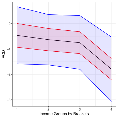
### Visual Description
## Line Chart: ACD vs. Income Groups by Brackets
### Overview
The image is a line chart showing the relationship between ACD (likely an acronym for a measured variable) and Income Groups by Brackets. The x-axis represents income groups, and the y-axis represents the ACD value. The chart displays a central tendency line (black) with upper and lower bounds indicated by red lines, and an overall uncertainty range indicated by blue lines.
### Components/Axes
* **X-axis:** "Income Groups by Brackets" with markers at 1, 2, 3, and 4.
* **Y-axis:** "ACD" with markers at -3, -2, -1, 0, and 1.
* **Data Series:**
* Black line: Represents the central tendency of ACD for each income group.
* Red lines: Represent the upper and lower bounds of a confidence interval around the central tendency.
* Blue lines: Represent the upper and lower bounds of a wider uncertainty range.
### Detailed Analysis
* **Income Group 1:**
* Black line (central tendency): Approximately -0.6
* Red lines (confidence interval): Approximately -0.9 and 0.0
* Blue lines (uncertainty range): Approximately -1.7 and 0.4
* **Income Group 2:**
* Black line (central tendency): Approximately -0.7
* Red lines (confidence interval): Approximately -1.1 and -0.1
* Blue lines (uncertainty range): Approximately -1.7 and 0.3
* **Income Group 3:**
* Black line (central tendency): Approximately -0.7
* Red lines (confidence interval): Approximately -1.2 and -0.2
* Blue lines (uncertainty range): Approximately -1.8 and 0.3
* **Income Group 4:**
* Black line (central tendency): Approximately -1.5
* Red lines (confidence interval): Approximately -2.2 and -0.9
* Blue lines (uncertainty range): Approximately -3.1 and -0.2
**Trends:**
* **Black Line (Central Tendency):** Relatively flat from Income Group 1 to 3, then decreases noticeably from Income Group 3 to 4.
* **Red Lines (Confidence Interval):** Both the upper and lower red lines are relatively flat from Income Group 1 to 3, then decrease from Income Group 3 to 4.
* **Blue Lines (Uncertainty Range):** The upper blue line is relatively flat from Income Group 1 to 3, then decreases from Income Group 3 to 4. The lower blue line is relatively flat from Income Group 1 to 2, then decreases sharply from Income Group 2 to 4.
### Key Observations
* The ACD value tends to decrease as the income group increases, particularly between groups 3 and 4.
* The uncertainty range (blue lines) is wider than the confidence interval (red lines), as expected.
* The confidence interval and uncertainty range appear to narrow slightly as income group increases.
### Interpretation
The chart suggests that there is a negative correlation between ACD and Income Groups by Brackets, especially at higher income brackets. The ACD value tends to be lower for higher income groups. The confidence interval and uncertainty range provide an indication of the variability in the data. The narrowing of the confidence interval and uncertainty range at higher income groups might suggest that the ACD value is more consistent within those groups. It is important to note that this is just a visual interpretation, and statistical analysis would be needed to confirm these observations.
</details>
(a) Partially Linear Model.
<details>
<summary>x8.png Details</summary>
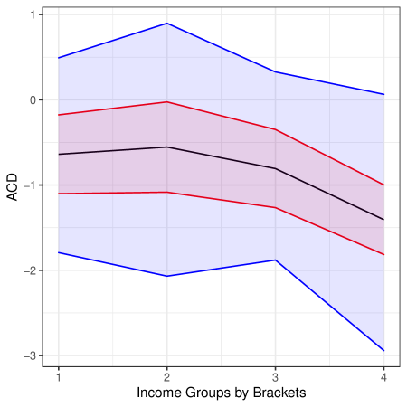
### Visual Description
## Line Chart: ACD vs. Income Groups by Brackets
### Overview
The image is a line chart displaying the relationship between ACD (likely an acronym for a measured variable) and Income Groups by Brackets. The chart includes a central black line representing the mean ACD value for each income group, a red shaded area indicating the standard error, and a blue shaded area indicating the standard deviation. The x-axis represents income groups, and the y-axis represents the ACD value.
### Components/Axes
* **X-axis:** "Income Groups by Brackets" with tick marks at 1, 2, 3, and 4.
* **Y-axis:** "ACD" with tick marks at -3, -2, -1, 0, and 1.
* **Mean:** Represented by a solid black line.
* **Standard Error:** Represented by a red shaded area around the mean.
* **Standard Deviation:** Represented by a blue shaded area around the mean.
### Detailed Analysis
* **Mean (Black Line):**
* At Income Group 1, the mean ACD is approximately -0.4.
* At Income Group 2, the mean ACD is approximately -0.3.
* At Income Group 3, the mean ACD is approximately -0.6.
* At Income Group 4, the mean ACD is approximately -1.4.
* Trend: The mean ACD is relatively stable between income groups 1 and 3, then decreases significantly at income group 4.
* **Standard Error (Red Shaded Area):**
* The red shaded area represents the standard error around the mean.
* At Income Group 1, the standard error ranges from approximately -0.2 to -1.2.
* At Income Group 2, the standard error ranges from approximately 0 to -1.1.
* At Income Group 3, the standard error ranges from approximately -0.2 to -1.4.
* At Income Group 4, the standard error ranges from approximately -0.8 to -2.0.
* Trend: The standard error appears to widen slightly as income group increases.
* **Standard Deviation (Blue Shaded Area):**
* The blue shaded area represents the standard deviation around the mean.
* At Income Group 1, the standard deviation ranges from approximately 0.4 to -1.8.
* At Income Group 2, the standard deviation ranges from approximately 0.9 to -2.1.
* At Income Group 3, the standard deviation ranges from approximately 0.3 to -1.9.
* At Income Group 4, the standard deviation ranges from approximately 0.1 to -2.9.
* Trend: The standard deviation appears to be relatively consistent across income groups, with a slight decrease at income group 4.
### Key Observations
* The mean ACD decreases as income group increases, particularly at income group 4.
* The standard error and standard deviation provide a measure of the variability of ACD within each income group.
* The standard deviation is larger than the standard error, as expected.
### Interpretation
The chart suggests that there is a relationship between income group and ACD. Specifically, as income group increases, the average ACD tends to decrease. The standard error and standard deviation indicate the degree of variability in ACD within each income group. The significant drop in ACD at income group 4 suggests that this income bracket may be associated with a different ACD pattern compared to the lower income groups. Further analysis would be needed to determine the statistical significance of these trends and the underlying factors driving the relationship between income group and ACD.
</details>
(b) Nonparametric Model.
Figure 6. One-Sided Confidence Bounds for the ACD by Income Brackets.
Note: Estimate (black), bounds (red), and confidence bounds (blue) for the ACD. Confounding scenario: $\rho^{2}=1$ ; $C^{2}_{Y}=0.03$ ; $C^{2}_{D}≈ 0.03$ . Significance level of 5%.
The second part of Table 5 reports the robustness values for price elasticity, such that the sensitivity bounds would contain a target value $\theta$ . Here we consider $\theta=-1.5$ (very elastic) and $\theta=0$ (perfectly inelastic). We find that, at the 5% confidence level, these robustness values are at around 2% (PLM) and 1% (NPM). These results show that, unless researchers are able to rule out confounding that explains at about 2% of the residual variation of gasoline price and gasoline consumption, the evidence provided by the data is not strong enough to distinguish between extremes such as a “very elastic,” or a “perfectly inelastic” demand function. To put this number in context, our coarse measure of income (median of the income bracket) explains around 15% of the residual variation of gasoline price and 7% of the residual variation of gasoline demand. It is thus not implausible that remnant variation in the true income could overturn these results.
Finally, we explore how price elasticity varies with income under a specific confounding scenario. We consider three overlapping income groups defined as observations with income within $±.5$ in log-scale around the income points $\$42,500$ , $\$57,500$ and $\$72,500$ , as well as a fourth high income group of all units with income above $11.6$ on the log scale ( $≈\$110,000$ ). To illustrate, we consider a confounding scenario of approximately 3% for both sensitivity parameters, and repeat our nonparametric and partially linear estimation and sensitivity analysis for each sub-group. Point-estimates, bounds and confidence bounds are reported in Figure 6. Note that, under this scenario, the evidence for effect heterogeneity is substantially weakened, especially when using a fully nonparametric model.