2201.12885

## Computational Metacognition Michael T. Cox Zahiduddin Mohammad Sravya Kondrakunta MICHAEL.COX@WRIGHT.EDU MOHAMMAD.48@ WRIGHT.EDU KONDRAKUNTA.2@WRIGHT.EDU Ventaksampath Raja Gogineni GOGINENI.14@WRIGHT.EDU Computer Science and Engineering, Wright State University, Dayton, OH 45435 USA Dustin Dannenhauer Othalia Larue DUSTIN.DANNENHAUER@PARALLAXRESEARCH.ORG OTHALIA.LARUE@PARALLAXRESEARCH.ORG Autonomy Research Group, Parallax Advanced Research, Beavercreek, OH 45431 USA ## Abstract Computational metacognition represents a cognitive systems perspective on high-order reasoning in integrated artificial systems that seeks to leverage ideas from human metacognition and from metareasoning approaches in artificial intelligence. The key characteristic is to declaratively represent and then monitor traces of cognitive activity in an intelligent system in order to manage the performance of cognition itself. Improvements in cognition then lead to improvements in behavior and thus performance. We illustrate these concepts with an agent implementation in a cognitive architecture called MIDCA and show the value of metacognition in problem-solving. The results illustrate how computational metacognition improves performance by changing cognition through meta-level goal operations and learning. ## 1. Introduction The computational metacognition process is analogous to an action-perception cycle in an intelligent agent (Cox, 2005). But, instead of perceiving the environment and acting in the world, metacognition monitors cognition and acts to control cognitive activity. In humans, such introspective processes can prove beneficial, as in a student's proper regulation of classroom learning (Price, Hertzog, & Dunlosky, 2009) or in a game show contestant's judgment of knowing answers to questions posed by the show's host (Reder & Ritter, 1992). Yet given the significant overhead and complexity it exhibits (Conitzer, 2011), metacognition is not a panacea for all computational tasks nor is it always beneficial in human performance (Norman, 2020; Wilson & Schooler, 1991). In this paper, we will examine the kinds of metacognitive activities that can improve a cognitive system's performance, and we will demonstrate these concepts in an implemented problem-solving domain. In some sense, metacognition is an add-on to a cognitive system. If a cognitive system has a certain behavior, then a metacognitive system should be able to observe that behavior and improve the performance of that system by changing its behavior given some parameters under its control. But here we are speaking of cognitive behavior (i.e., problem solving) rather than the physical behavior of the system in the world. The impact on the actual behavior of the joint system is indirect and improves performance by improving thinking. As such, metacognition is one of the characteristics of intelligence that separates humans from mere reinforcement machines. This paper presents a computational approach to metacognition that seeks to clarify the manner in which such indirect levers can exert such influential effects on performance. Its contribution is to specify the mechanism of metacognition in computational terms within the context of an existing cognitive architecture and to evaluate these concepts in planning problems. Previous work has discussed the process of detecting metacognitive expectation failures; the paper here discusses the processes of meta-level explanation and goal generation as well as meta-level planning and learning. This is our first fully complete implementation of the metacognitive cycle. Section 2 describes our concept of computational metacognition consisting of explanatory, immediate and anticipatory metacognition. Subsequently, Section 3 shows how a cognitive architecture instantiates many of these ideas computationally and illustrates the principles with examples. Section 4 then evaluates this approach empirically in a simple, plant-protection domain. Finally, Section 5 enumerates related research, and Section 6 summarizes and concludes. ## 2. Computational Metacognition Though the concept of computational metacognition has many variations in the literature, having both broad and narrow interpretations, virtually all theories divide it into some kind of introspective monitoring and meta-level control . In the broader sense, any self-directed process can be included under its umbrella; whereas, the stricter definition of meta-x as 'x about x' (see Hayes-Roth, Waterman, & Lenat, 1983) constrains the subject to cognition about cognition. This more narrow definition excludes related concepts such as meta-knowledge (i.e., knowledge about knowledge) which is not a cognitive process per se (Cox, 2011). But broadly speaking in all its interpretations across the literature, metacognition is surely 'the many-headed monster of obscure parentage' of which Brown (1987) speaks; it is not a single monolithic construct. Instead, we claim that metacognition has three fundamental forms (see Table 1). Table 1 . Types of Computational Metacognition | Explanatory | Immediate | Anticipatory | |---------------|---------------|----------------| | Past | Present | Future | | Hindsight | Insight | Foresight | | Retrospective | Introspective | Predictive | Explanatory metacognition is a reflective process triggered by failures in previous cognitive operations and thus represents a process akin to hindsight. Immediate metacognition represents introspective run-time control of cognition, analogous to physical eye-hand coordination. 1 Anticipatory metacognition is a reflective judgement of future cognitive performance and hence represents self-directed foresight. This paper has little room to discuss all three forms. Instead, it will focus on the explanatory category of metacognition and briefly examine the anticipatory one. 1 This is also related to decision-theoretic metareasoning applied to partial computations (Horvitz, 1990) and to bounded rationality decisions for anytime-planning (Zilberstein, 2011). In contrast, our approach is symbolic and non-statistical. ## COMPUTATIONAL METACOGNITION ## 2.1 Explanatory Metacognition Expectations play important functional roles in cognition such as the monitoring of plan execution (Dannenhauer & Munoz-Avila, 2015; Pettersson, 2005; Schank, 1982), managing comprehension, especially natural language understanding (Schank & Owens, 1987), and influencing emotion (Langley, 2017). Expectations are knowledge artifacts that enable cognitive systems to verify their behavior is working as intended. The agent checks if discrepancies exist between its expectations and its observations of the state of the world. When such a discrepancy is detected, an expectation failure is said to occur. Different means of addressing expectation failures have been proposed including plan adaptation (i.e., modifying a plan to be executed) (Munoz-Avila & Cox, 2008), learning (i.e., acquiring a new piece of knowledge) (Munoz-Avila, 2018; Ram & Leake, 1995a), and goal reasoning (i.e., changing the goals pursued or formulating new goals to be achieved) (Aha, 2018; Roberts, Borrajo, Cox, & Yorke-Smith, 2018). Expectation failures are signals that a problem may have arisen. Explanations of the problem then provide the basis for goal formulation and thus facilitate problem-solving. Note that we are referring to a kind of internal explanation or selfdiagnosis process rather than an external explanation to another agent. Similarly, metacognitive expectations (Dannenhauer, Cox, & Munoz-Avila, 2018) play an analogous role to the expectations discussed above. But here the expectation concerns the outcome of cognitive processes rather than events in the world. As such, it relates the mental states immediately before and resulting from a specific mental process or action. An individual mental state 𝑠𝑠 𝑀𝑀 = ( 𝑣𝑣1 , … , 𝑣𝑣 𝑛𝑛 ) is a vector of variables; whereas, a mental action 𝛼𝛼 𝑀𝑀 performs reads from or updates to variables in a mental state. The metacognitive expectation then is represented as the triple ( 𝑠𝑠 𝑖𝑖 𝑀𝑀 , 𝛼𝛼 𝑖𝑖 𝑀𝑀 , 𝑠𝑠 𝑖𝑖+1 𝑀𝑀 ) where 𝛼𝛼 𝑖𝑖 𝑀𝑀 is the current cognitive process and each 𝑠𝑠 𝑀𝑀 represents the system's mental state immediately preceding and following from it. 2 That is, for a given cognitive process, the expectation specifies constraints on memory associated with the execution of the process. For example, one might expect commitment to a current goal before a planning process and a plan to be in memory after planning finishes. That is, the expectation would be represented as the triple ( 𝑔𝑔 𝑐𝑐 ∈ 𝑠𝑠 𝑖𝑖 𝑀𝑀 , 𝑃𝑃𝑃𝑃𝑃𝑃𝑃𝑃 , 𝜋𝜋 ∈ 𝑠𝑠 𝑖𝑖+1 𝑀𝑀 ) . If a plan does not result after planning executes, then something went wrong in cognition (Cox & Dannenhauer, 2016). The reasoning from such metacognitive expectation failures is in hindsight, because it happens after a mistake occurs. The function of metacognition is to explain what caused the cognitive-level failure and to formulate a meta-level goal to mitigate the problem. For example, changing the goal minimally to something easier but serving the same end may enable successful planning when physical resources are scarce (see Cox & Veloso, 1998). Multiple meta-level goals are available to affect cognition. Currently, we have implemented three different meta-level goal types. The first aims to change cognition directly, while the other two represents indirect change. 1. To change the reasoning method (e.g., change from state-space planning to case-based planning) (Cox & Dannenhauer, 2016); 2. To change cognition by changing the goals of the system (Cox, Dannenhauer, & Kondrakunta, 2017); 3. To change cognition by learning new knowledge structures (Mohammad, 2021; Mohammad, Cox, & Molineaux, 2020). 2 Dannenhauer, et al. (2018) defined metacognitive expectations as a Boolean function taking such a triple as input. But, the differences are unimportant for the purposes of this paper. This paper will focus on the third type, that is, learning-goals (i.e., an explicit meta-level goal to learn a specific piece of knowledge) (Cox, 1997; Cox & Ram, 1999; Ram & Leake, 1995b) as a metacognitive response, but the others are equally as important. Plans can be generated at the metalevel composed of 'actions' such as performing learning in pursuit of a learning goal or executing different goal operations (Cox, et al., 2017; Kondrakunta, Gogineni, & Cox, in press) such as goal change in pursuit of the second type above. But, the goal delegation operation has a particular role in anticipatory metacognition which spans both cognition and metacognition. ## 2.2 Anticipatory Metacognition The concept of anticipatory metacognition is forward looking. Humans demonstrate foresight concerning their cognitive prowess or the lack thereof on a regular basis. Likewise, cognitive systems can benefit from an ability to predict whether or not they can achieve their goals as opposed to exhaustively trying all possible solutions before acquiescing. Unlike anticipatory thinking (Amos-Binks & Dannenhauer, 2019) that predicts plan execution failures and seeks to mitigate the vulnerability of a plan after it is generated, our approach is to anticipate a failure given the goal but before planning is performed. Making such a prediction, an agent can simply delegate some of its goals to another agent willing to help it and thus mitigate the amount of work to be done. In contrast to explanatory metacognition, which is triggered by metacognitive expectation failures, anticipatory metacognition is triggered by the presence of suspended goals . Suspended goals are ones that were part of an agent's current goal set but were determined to be problematic given physical resource limitations for example. This condition suggests that planning or other reasoning will fail in the future. As a result, metacognition can generate a meta-level goal to change the cognitive-level goal. In this case, it is a change from the agent's goal to another agent's goal. Thus, the goal delegation operation is partially performed at the cognitive level and partially at the meta-level. Suspending the goal is cognitive; whereas, reasoning about another agent's knowledge, skills and goals in relation to the agent's own goals is associated with Theory of Mind (Goldman, 2006; Gopnik, 2012; Wellman, 1990) and with metacognition. This allows the system to target a good candidate agent for the delegation. Finally, if the agent decides to delegate one or more of its goals and determines a candidate to achieve them, the agent still needs to make an actual request, explain the need for the request, and negotiate the favor. Such reasoning is once again situated at the cognitive level and in the speech acts (Searle, 1969) executed in the world. Gogineni, Kondrakunta, and Cox (in press) provide a complete example of this hybrid process with experimental evidence supporting the benefits of this type of metacognitive activity. Given space limitations, this paper cannot but sketch the mechanisms behind anticipatory metacognition. Instead, we will describe the detailed process of explanatory metacognition and show how it is implemented in a particular cognitive architecture. Specifically, we will explain how it manifests as a combination of introspective monitoring and meta-level control. With these details in hand, we will then provide an empirical evaluation that demonstrates the benefit of computational metacognition for cognitive systems. ## 3. Architectural Structure and Implementation The metacognitive integrated dual-cycle architecture (MIDCA) is a cognitive architecture that models both cognition and metacognition for intelligent agents (Cox et al., 2016; Cox, Oates, & Perlis, 2011; Paisner, Cox, Maynord, & Perlis, 2014) and focusses upon various goal operations including goal change, goal formulation and goal delegation (Cox & Dannenhauer, 2017; Cox, et ## COMPUTATIONAL METACOGNITION 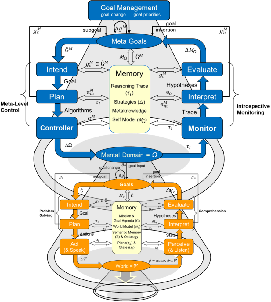al., 2017). 3 It consists of 'action-perception' cycles at both the cognitive level and the metacognitive level (see Figure 1). In general, a cycle performs problem-solving to achieve its goals and then comprehends the results of its behavior and interactions with other agents in its environment. The problem-solving portion of each cycle consists of three phases: intention; planning; and the action-execution/control phase. The comprehension portion consists of perception/monitoring, interpretation, and goal evaluation. The representations in MIDCA and our formal notation borrow much from the AI planning community (e.g., Ghallab, Nau, Traverso, 2004). We rely on the notion of a state transition system Σ = ( 𝑆𝑆 , 𝐴𝐴 , 𝛾𝛾 ) for representing a planning problem. In Σ , 𝑆𝑆 is the set of all possible world states, 𝐴𝐴 is the set of actions the agent can take, and 𝛾𝛾 is the successor function 𝛾𝛾 : 𝑆𝑆 × 𝐴𝐴 ⇢ 𝑆𝑆 . A planning problem is represented as 𝒫𝒫 = ( Σ , 𝑠𝑠0 , 𝑔𝑔 ) where the initial state 𝑠𝑠0 ∈ 𝑆𝑆 and the goal 𝑔𝑔 ∈ 𝐺𝐺 ⊂ 𝑆𝑆 . A plan 𝜋𝜋 = 〈𝛼𝛼1 , 𝛼𝛼2 , … , 𝛼𝛼 𝑛𝑛 〉 is a sequence of actions 𝛼𝛼 𝑖𝑖 ∈ 𝐴𝐴 . The plan 𝜋𝜋 represents a solution to 𝒫𝒫 by achieving 𝑔𝑔 if and only if its iterative execution from 𝑠𝑠0 results in a final state 𝛾𝛾 ( 𝑠𝑠 𝑛𝑛-1 , 𝛼𝛼 𝑛𝑛 ) that entails the goal expression. Note however, that a problem need not always start from some arbitrary initial state but instead may arise during the planning or the plan execution related to some previous problem (Cox, 2020). 4 At the cognitive level, comprehension starts with observations in terms of percepts ( 𝑝𝑝 ⃑ ) of the world ( 𝛹𝛹 ) whereby the Perceive phase infers the objects in the environment and the relationships between them. The Interpret phase takes as input the resulting relational state ( 𝑠𝑠 𝑗𝑗 ) and the expectations in memory to determine whether it is making sufficient progress. It is here that a model of the world ( 𝑀𝑀Ψ ) is inferred from its observations, and new goals ( 𝑔𝑔 𝑛𝑛 ) are generated when the model indicates problems or opportunities. Interpret adds any new goals to the goal agenda ( 𝐺𝐺 � = { 𝑔𝑔1 , 𝑔𝑔2 , … 𝑔𝑔 𝑛𝑛 } ). The Evaluate phase incorporates the concepts inferred from Interpret and checks whether the current goal set ( 𝑔𝑔 𝑐𝑐 ∈ 𝐺𝐺 � ) is achieved, i.e., whether 𝑠𝑠 𝑗𝑗 entails 𝑔𝑔 𝑐𝑐 . If so, 𝑔𝑔 𝑐𝑐 is removed from the agenda and set to the empty set (i.e., 𝐺𝐺 � ← 𝐺𝐺 � / 𝑔𝑔 𝑐𝑐 and 𝑔𝑔 𝑐𝑐 ← {} ). In cognitive-level problem solving, the Intend phase commits to a new goal set 𝑔𝑔 𝑐𝑐 from those available in 𝐺𝐺 � if the old goal set is empty. The Plan phase then generates a sequence of actions (i.e., the current plan, 𝜋𝜋 𝑘𝑘 = 〈𝛼𝛼1 , 𝛼𝛼2 , … 𝛼𝛼 𝑛𝑛 〉 ) to perform in pursuit of its goals. The Act phase executes the steps of the plan ( 𝛼𝛼 𝑖𝑖 ) one at a time to change the environment through their effects. MIDCA will then use expectations about these actions in subsequent cycles to evaluate the execution of the plan. At the end of each cognitive phase, MIDCA performs an entire metacognitive cycle as explained below. Like cognition, MIDCA partitions metacognition into introspective monitoring (analogous to cognitive-level comprehension) and meta-level control (analogous to problem-solving). Introspective monitoring detects metacognitive expectation failures and formulates goals to change cognition in response. Meta-level control generates and executes plans to achieve these goals and thus improve cognitive performance. See Dannenhauer, et al. (2018) for a more formal specification of the two-cycle MIDCA mechanism. Here we give enough detail to capture the metacognitive process computationally and allow the reader to follow the examples and understand the evaluation. 3 MIDCA version 1.5 is open-source and runs on python 3.8. The source code and documentation are publicly available at https://github.com/COLAB2/midca. See also www.midca-arch.org . 4 We actually assume a somewhat different problem representation 𝒫𝒫 𝑐𝑐 = ( 𝑠𝑠 𝑐𝑐 , 𝑠𝑠 𝑒𝑒 , 𝐵𝐵𝐵𝐵 , 𝐻𝐻 𝑐𝑐 ) where 𝑠𝑠 𝑐𝑐 and 𝑠𝑠 𝑒𝑒 represent the currently observed and expected world states, 𝐵𝐵𝐵𝐵 is the background knowledge and 𝐻𝐻 𝑐𝑐 is the episodic problemsolving history of the agent (see Cox, 2020). But the differences are not important for the purposes of this paper and may be ignored by the reader. Figure 1 . The metacognitive integrated dual-cycle architecture and the flow of knowledge between computational phases. The lower (orange) cycle represents cognition, receiving stimuli in the form of percepts and acting upon the environment, thus changing the world state. The upper (blue) cycle represents metacognition, receiving an introspective trace of cognition and controlling the cognitive level through goal operations and learning. Note that all knowledge structures 𝐵𝐵 that are metacognitive have the superscript 𝐵𝐵 𝑀𝑀 . <details> <summary>Image 1 Details</summary>  ### Visual Description ## Cognitive Architecture Diagram ### Overview The image presents a cognitive architecture diagram, illustrating the flow of information and processes within a cognitive system. It depicts two levels of processing: a meta-level control and a problem-solving level, along with introspective monitoring. The diagram uses boxes to represent cognitive modules, arrows to indicate the flow of information, and labels to describe the processes and data involved. ### Components/Axes The diagram is structured around two main processing loops: Meta-Level Control (top, in blue) and Problem Solving (bottom, in orange). Introspective Monitoring is shown on the right side. **Key Components:** * **Goal Management:** Located at the top-center, with inputs "goal change" and "goal priorities". * **Meta Goals:** A central node in the meta-level control loop. * **Intend (Meta-Level):** A module in the meta-level control loop. * **Plan (Meta-Level):** A module in the meta-level control loop. * **Controller:** A module in the meta-level control loop. * **Mental Domain = Ω:** A central node connecting the meta-level and problem-solving loops. * **Goals:** A central node in the problem-solving loop. * **Intend (Problem-Solving):** A module in the problem-solving loop. * **Plan (Problem-Solving):** A module in the problem-solving loop. * **Act (& Speak):** A module in the problem-solving loop. * **World = Ψ:** The external environment. * **Memory (Meta-Level):** Contains "Reasoning Trace (τl)", "Strategies (Δ)", "Metaknowledge", and "Self Model (MΩ)". * **Memory (Problem-Solving):** Contains "Mission & Goal Agenda (Ĝ)", "World Model (Mψ)", "Semantic Memory (Σ) & Ontology", and "Plans(πk) & States(sj)". * **Evaluate (Meta-Level):** A module in the meta-level control loop. * **Interpret (Meta-Level):** A module in the meta-level control loop. * **Monitor:** A module for introspective monitoring. * **Evaluate (Problem-Solving):** A module in the problem-solving loop. * **Interpret (Problem-Solving):** A module in the problem-solving loop. * **Perceive (& Listen):** A module in the problem-solving loop. **Arrows and Labels:** * Arrows indicate the direction of information flow. * Labels on arrows describe the type of information being passed (e.g., "goal", "algorithms", "actions", "hypotheses", "trace"). * Variables are used to represent specific data or states (e.g., gM, ΔgM, MΩ, τl, πk, Ψ). ### Detailed Analysis or ### Content Details **Meta-Level Control Loop (Blue):** 1. **Goal Management** feeds into **Meta Goals**. 2. **Meta Goals** sends information to **Intend**. 3. **Intend** passes a "Goal" to **Plan**. 4. **Plan** generates "Algorithms" for the **Controller**. 5. **Controller** influences the **Mental Domain = Ω** via ΔΩ. 6. **Meta Goals** exchanges information with **Memory (Meta-Level)** via G^M. 7. **Memory (Meta-Level)** sends information to **Evaluate**. 8. **Evaluate** passes "Hypotheses" to **Interpret**. 9. **Interpret** sends "Trace" to **Monitor**. 10. **Monitor** sends τl back to **Memory (Meta-Level)**. **Problem-Solving Loop (Orange):** 1. **Mental Domain = Ω** influences **Goals**. 2. **Goals** sends information to **Intend**. 3. **Intend** passes a "Goal" to **Plan**. 4. **Plan** generates "Actions" for **Act (& Speak)**. 5. **Act (& Speak)** interacts with the **World = Ψ** via ΔΨ. 6. **Goals** exchanges information with **Memory (Problem-Solving)** via G. 7. **Memory (Problem-Solving)** sends information to **Evaluate**. 8. **Evaluate** passes "Hypotheses" to **Interpret**. 9. **Interpret** sends "State" to **Perceive (& Listen)**. 10. **Perceive (& Listen)** interacts with the **World = Ψ** via p = noise, ψ ⊂ Ψ. **Introspective Monitoring (Right Side):** * The **Monitor** receives "Trace" from **Interpret (Meta-Level)**. * The **Monitor** sends τl to **Memory (Meta-Level)**. ### Key Observations * The diagram highlights the interaction between meta-level control and problem-solving processes. * Memory plays a crucial role in both loops, storing information and influencing decision-making. * The Mental Domain acts as a bridge between the two levels. * Introspective monitoring allows the system to reflect on its own processes. * The World represents the external environment, which the system interacts with through perception and action. ### Interpretation This cognitive architecture diagram illustrates a hierarchical cognitive system capable of both problem-solving and meta-level reasoning. The meta-level control loop allows the system to manage its goals, strategies, and knowledge, while the problem-solving loop focuses on interacting with the environment and achieving specific tasks. The introspective monitoring component enables the system to evaluate its own performance and adapt its strategies accordingly. The diagram suggests a system that can learn and improve over time by reflecting on its experiences and updating its internal models. The interaction between the different modules and levels of processing allows for flexible and adaptive behavior. The inclusion of "noise" in the interaction with the "World" acknowledges the uncertainty and complexity of real-world environments. </details> ## 3.1 Introspective Monitoring At the meta-level, introspective monitoring starts with a trace ( 𝜏𝜏 𝑙𝑙 ) of the mental domain, that is, of the activity at the cognitive level (again see Figure 1). In support of this knowledge structure, Dannenhauer, et al., (2018) defines an agent's self-model (i.e., a model of the cognitive level) as Ω = ( 𝑆𝑆 𝑀𝑀 , 𝐴𝐴 𝑀𝑀 , 𝜔𝜔 ) where each 𝑠𝑠 𝑖𝑖 𝑀𝑀 ∈ 𝑆𝑆 𝑀𝑀 is a possible mental state, each 𝛼𝛼 𝑖𝑖 𝑀𝑀 ∈ 𝐴𝐴 𝑀𝑀 is a mental action, and 𝜔𝜔 is a cognitive transition function. 5 In MIDCA, a mental state is represented as a vector of length 𝑃𝑃 = 7 where 𝑠𝑠 𝑖𝑖 𝑀𝑀 = ( 𝑔𝑔 𝑐𝑐 , 𝐺𝐺 � , 𝜋𝜋 𝑘𝑘 , 𝑀𝑀Ψ , 𝐷𝐷 , 𝐸𝐸 , 𝛼𝛼 𝑖𝑖 ) . That is, it consists of the current goal, the goal agenda, the current plan, the current world state, discrepancies detected, explanations generated, and the last action executed in the world. MIDCA employs the following mental actions: Perceive, Detect Discrepancies, Explanation, Goal Insertion (i.e., updates the set of goals 𝐺𝐺 � to be achieved), Evaluate, Intend, Plan, and Act. Each of these represent either one of the six phases at the cognitive level or a subprocess within Interpret. The cognitive transition function is defined as 𝜔𝜔 : 𝑆𝑆 𝑀𝑀 × 𝐴𝐴 𝑀𝑀 ⟶𝑆𝑆 𝑀𝑀 . That is, given a current mental state, 𝜔𝜔 provides the successive mental state resulting from the execution of that mental action and hence is a source of metacognitive expectations. Finally, the trace is an interleaved sequence of mental states and mental actions. More specifically, 𝜏𝜏 𝑙𝑙 = 〈𝑠𝑠0 𝑀𝑀 , 𝛼𝛼1 𝑀𝑀 , 𝑠𝑠1 𝑀𝑀 , 𝛼𝛼2 𝑀𝑀 , … , 𝛼𝛼 𝑛𝑛 𝑀𝑀 , 𝑠𝑠 𝑛𝑛 𝑀𝑀 〉 where 𝑠𝑠0 𝑀𝑀 , … , 𝑠𝑠 𝑛𝑛 𝑀𝑀 ∈ 𝑆𝑆 𝑀𝑀 and 𝛼𝛼1 𝑀𝑀 , … , 𝛼𝛼 𝑛𝑛 𝑀𝑀 ∈ 𝐴𝐴 𝑀𝑀 . The Monitor phase takes the recorded trace and places it in memory for the meta-level Interpret phase to examine. As with the cognitive level phase, meta-level Interpret seeks to detect and explain discrepancies between specific metacognitive expectations and its 'observations' in segments of the cognitive trace. As mentioned in Section 2.1 these expectations consist of the memory states before and after a given cognitive phase or phase component. If a discrepancy exists, then Interpret attempts to explain the discrepancy and formulate a meta-level goal. Consider an agent that is learning to take care of a garden having goals such as the preservation of native plants and the removal of invasive ones. Its knowledge of plant care, such as the correct application of herbicide, may be flawed, and therefore it may make mistakes in both the execution of solutions (i.e., its behavior in the world) and in the derivation of those solutions (i.e., its reasoning to solve problems). For example, the agent's model of the spray action may lack the knowledge that spraying herbicide will kill plants in locations adjacent to those it targets. When the goal of native plant preservation is violated after spraying invasive ones close to the natives, a normal discrepancy occurs. However, when the Interpret phase fails to explain this discrepancy, a metacognitive expectation fails. That is, the cognitive trace 𝜏𝜏 𝑙𝑙 does not adhere to the expectation ( 𝑑𝑑𝑑𝑑𝑠𝑠𝑑𝑑𝑑𝑑𝑑𝑑𝑝𝑝𝑃𝑃𝑃𝑃𝑑𝑑𝑑𝑑 ∈ 𝑠𝑠 𝑖𝑖 𝑀𝑀 , Explain , 𝑑𝑑𝑒𝑒𝑝𝑝𝑃𝑃𝑃𝑃𝑃𝑃𝑃𝑃𝑒𝑒𝑑𝑑𝑒𝑒𝑃𝑃 ∈ 𝑠𝑠 𝑖𝑖+1 𝑀𝑀 ) since the Explain component of the Interpret phase failed to produce the expected explanation. 6 Now the discrepancy at the metalevel must be explained. 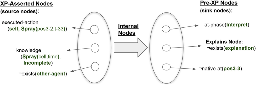At the meta-level Interpret phase, the idea is to detect discrepancies, explain what caused the discrepancy, and then generate a goal to remove the cause. Metacognitive explanation is a casebased process that reuses old explanations from a library of meta-explanation patterns (Meta-XPs) in a similar manner to Cox and Ram (1999; Ram & Cox, 1994). Figure 2 shows a Meta-XP applied to the gardening example. MIDCA retrieves an explanation and then checks for applicability by inspecting the Meta-XP's pre-XP nodes. These sink nodes in the graph of the knowledge structure represent those conditions that need to hold for the XP to be relevant. A distinguished node among them called the Explains node is the concept being explained. As such, the XP provides a causal 5 The self-model Ω is similar to the state transition system Σ defined previously but is a meta-level knowledge structure. 6 Note that if another gardener was observed concurrently spraying herbicide on the adjacent native plant, then an explanation as to why the native plant was killed could be produced and a goal to stop the gardener from repeating that in the future formulated. If this actually was the case, then no metacognitive expectation failure would occur. ## COMPUTATIONAL METACOGNITION Figure 2 . Meta-explanation pattern for failed action execution due to a poor action model. An explanation pattern (Schank, 1986) is a causal knowledge structure representing prior experience. It maps the causes of the explains node (i.e., what is being explained) from the antecedents (i.e., the XP-asserted nodes) through the internal nodes to the consequents (i.e., the pre-XP nodes). <details> <summary>Image 2 Details</summary>  ### Visual Description ## Diagram: Node Relationships ### Overview The image is a diagram illustrating the relationship between "XP-Asserted Nodes" (source nodes) and "Pre-XP Nodes" (sink nodes) through "Internal Nodes". It depicts a flow or connection between these node types, with specific examples of the content within each node. ### Components/Axes * **XP-Asserted Nodes (source nodes):** Located on the left side of the diagram. * Contains three nodes with the following information: * executed-action (self, Spray(pos3-2,t-33)) * knowledge (Spray(cell,time), Incomplete) * ¬exists(other-agent) * **Internal Nodes:** Positioned in the center of the diagram, represented by a gray arrow pointing from left to right. * **Pre-XP Nodes (sink nodes):** Located on the right side of the diagram. * Contains three nodes with the following information: * at-phase(Interpret) * Explains Node: ¬exists(explanation) * ¬native-at(pos3-3) ### Detailed Analysis * **XP-Asserted Nodes:** * The "executed-action" node contains the action "Spray" at position "pos3-2" and time "t-33". * The "knowledge" node contains information about "Spray" with cell and time parameters, and it's marked as "Incomplete". * The "¬exists(other-agent)" node indicates the absence of another agent. * **Internal Nodes:** * Represented by a gray arrow, indicating a flow or transformation between the source and sink nodes. * **Pre-XP Nodes:** * The "at-phase(Interpret)" node indicates the interpretation phase. * The "Explains Node: ¬exists(explanation)" node suggests the absence of an explanation. * The "¬native-at(pos3-3)" node indicates the absence of a native element at position "pos3-3". ### Key Observations * The diagram illustrates a flow from XP-Asserted Nodes to Pre-XP Nodes through Internal Nodes. * The nodes contain information about actions, knowledge, and existence or absence of certain elements. * The "Spray" action and position "pos3" are mentioned in both XP-Asserted and Pre-XP Nodes, suggesting a connection or transformation of information. ### Interpretation The diagram represents a simplified model of how information flows and is transformed within a system. The XP-Asserted Nodes act as the source of information, which is then processed or transformed through Internal Nodes to arrive at the Pre-XP Nodes. The specific content within each node provides insights into the nature of the information being processed, such as actions, knowledge, and existence conditions. The diagram could be used to illustrate the reasoning process of an AI agent, where the agent starts with certain beliefs (XP-Asserted Nodes), infers new information (Internal Nodes), and arrives at conclusions (Pre-XP Nodes). The presence of negations (¬exists) suggests that the system is also capable of reasoning about the absence of certain elements. </details> chain from the XP-asserted nodes (i.e., the XP's antecedents) to the explains node. In the running example, the Meta-XP of Figure 2 explains why the cognitive level Interpret phase failed to generate an explanation when MIDCA was currently at the Interpret phase and a native-plant was not preserved. If that is the case, then the XP says that this is caused when the spray action was executed, no other agent exists nearby, and knowledge of the spray action is incomplete. The meta-level Interpret phase then takes this knowledge structure and generates a goal from the set of XP-asserted nodes. Here the goal is to negate the middle node, that is, to make the knowledge of the spray operator not incomplete (i.e., to learn a better action model). The specific form output to the meta-level goal agenda is (learned spray, 𝑠𝑠 𝑖𝑖+1 ) . See Gogineni, Kondrakunta, Molineaux, & Cox (2018) for further details concerning XP retrieval, selection and application at the cognitive level. The same techniques are used at the meta-level. ## 3.2 Meta-level Control Like problem-solving at the cognitive level, meta-level control consists of an Intend phase, a metalevel Plan phase, and a Controller. Intend takes the meta-level goal agenda ( 𝐺𝐺 � 𝑀𝑀 ) and chooses a subset as the current meta-level goal set ( 𝑔𝑔 𝑐𝑐 𝑀𝑀 ). Details are available in Kondrakunta and Cox (in press; Kondrakunta, 2017) for the decision mechanism. In our running example, only the single learning goal exists in the agenda, and so Intend selects it as the current goal set. The Plan phase of the meta-level then takes the current goals and generates a plan 𝜋𝜋 𝑚𝑚 𝑀𝑀 to achieve it using the fast-downward stone soup planner (Helmert, 2006; Helmert, Roger, & Karpas, 2011). Unlike normal planners that generate sequences of actions in the world to achieve environmental states, MIDCA uses fast downward to achieve meta-level goals. Given the learning goal (learned spray 𝑠𝑠 𝑖𝑖+1 ) , Fast Downward must generate a sequence of learning steps that achieves the goal if executed. To perform this task, MIDCA has a number of operators represented in the Planning Domain Definition Language (PDDL) 2.2 (Edelkamp & Hoffmann, 2004), one of which is shown in Table 2. To select the perform-learning action, the agent checks whether it has a Table 2 . Action model of the meta-level operator perform-learning . Specified in PDDL 2.2, this primitive, planning operator achieves the learning goal (learned ?op ?current-state) . ``` ``` discrepancy in the current state, it has an outdated operator, and the same operator caused the discrepancy. If all the preconditions are met, then it results in the learning goal. The Controller then attempts to execute the plan one step 𝑃𝑃 𝑛𝑛 𝑀𝑀 at a time. In the example, the plan has a single step to perform learning. MIDCA uses the First-Order Inductive Learner (FOIL) (Quinlan, 1990) for this paper. FOIL induces function-free Horn clauses from a set of positive and negative concept examples and some background knowledge represented as a set of first-order logical predicates. It performs hill climbing with an information theoretical function and generates a rule that covers all the examples. The FOIL algorithm is given positive or negative examples experienced during the execution of failed plans. For example, the spray action may have killed a plant in a location directly north of the intended cell. If so, FOIL will learn the following general Horn clause. spray (pos1, time2) :- spray (pos0, time1), adj\_time (time2, time1), adj\_north (pos0, pos1) That is, if the agent sprays a location at time t1, it will be as if it sprays the adjacent location due north at t2. Doing so will then kill all plants in the cell north of the spray. MIDCA then compares such rules generated by the learning procedure with the agent's knowledge of the operator. As a result, it changes the spray operator by adding conditional effects. ``` ``` After the agent's memory is updated with the modified operator, the metacognitive cycle ends. Once metacognition completes, MIDCA continues with the subsequent cognitive phase. Given an incrementally improved operator as with our example or otherwise with some other positive change to cognition, performance will improve. The following section examines this claim empirically and shows specific benefits to cognitive systems that reason about themselves. ## 4. Empirical Evaluation We evaluate the claim that metacognition can improve the performance of cognitive systems with a relatively simple planning task. The experiments we perform use the plant protection domain developed at the Naval Research Laboratory. 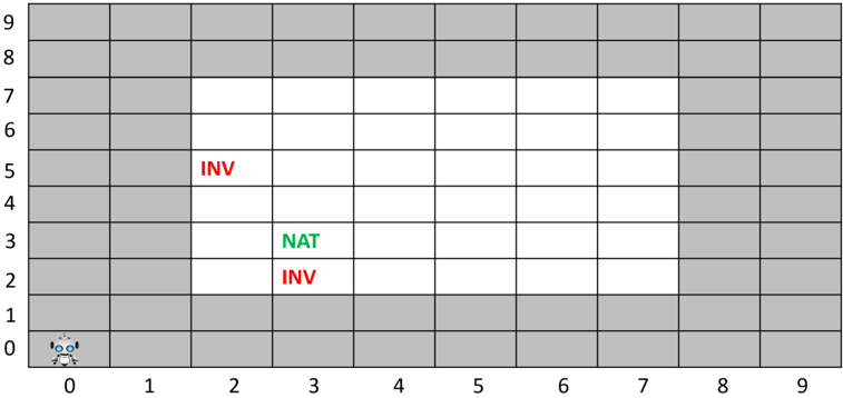## 4.1 The Plant Protection Domain The plant protection domain consists of harmful invasive plants, endangered native plants, a human supervisor, and an agent which navigates to a target cell and deploys herbicides (Boggs, Dannenhauer, Floyd, & Aha, 2018). When an agent deploys herbicides, it will affect the neighboring cells as well. The world in which agents act is a map grid of size 10 ⨉ 10, as shown in Figure 3. It consists of tiles where a plant occupies a single tile, and the tiles contain at most one plant. Plants are static fixtures that cannot be moved or replanted. The garden area where plants exist lies between (2,2) and (7,7), i.e., the white rectangle. In this domain, two key action models exist: a move operator and a spray operator. The walkway around the planting area exists for the ease of agent movement. Figure 3 visually depicts a very simple problem with a gardening agent at location (0,0). The goals of the agent are to preserve all native plants and to remove all invasive ones, i.e., nativeat(pos3-3) ∧ ¬invasive-at(pos2-5) ∧ ¬invasive-at(pos3-2) . Here, the Perceive phase of the cognitive cycle inputs the requested expression for the goals, Interpret adds these goals to the goal agenda, and Intend makes all goals current. Finally, the Plan phase takes the current goal set and generates a plan to move to location (3,2), spray the invasive plant, move to location (2,5), and spray again. Given that the native plant already exists at location (3,3) in the initial state, nothing needs to be done to achieve the goal to have a native plant at (3,3). However, the agent does not realize that spraying in one cell will kill plants in all adjacent cells. Thus, the native plant in (3,3) is also killed. ## 4.2 Experimental Design Two experiments provide a baseline for determining how metacognition with learning affects the performance of an agent in the plant protection domain. Our tests were run in the 10 × 10 world (as discussed above) with a standard planning agent and a metacognitive learning agent. The standard agent does not perform goal reasoning or learning. It just executes plans to remove all invasives. The learning agent learns a more accurate model of its actions over the range of goals given and can reject harmful goals accordingly. We randomly place invasive and native plants in the map grid to form problems of increasing difficulty (i.e., larger amounts of invasive plants and hence more goals to solve in a problem). ## COMPUTATIONAL METACOGNITION Figure 3 . A simple problem in the plant protection domain. The central rectangular area in white indicates the garden with native and invasive plants represented by the symbols NAT and INV respectively. The gardening agent at the origin needs to remove invasives and preserve native plants. <details> <summary>Image 3 Details</summary>  ### Visual Description ## Grid World Diagram ### Overview The image depicts a 10x10 grid world environment. Some cells are grayed out, representing obstacles or boundaries, while others are white, indicating traversable space. A small robot icon is located in the bottom-left corner (0,0). The grid also contains labels "INV" (in red) and "NAT" (in green) at specific locations. ### Components/Axes * **Grid:** 10x10 grid, with rows and columns numbered 0-9. * **Robot:** A small robot icon located at grid coordinate (0,0). * **Obstacles/Boundaries:** Grayed-out cells representing impassable areas. * **Labels:** * "INV" (red) at (2,5) * "NAT" (green) at (3,3) * "INV" (red) at (3,2) ### Detailed Analysis or ### Content Details The grid world has the following characteristics: * **Dimensions:** 10 rows and 10 columns, indexed from 0 to 9. * **Robot Starting Position:** The robot is located at the bottom-left corner, coordinate (0,0). * **Obstacle Configuration:** * Row 0 (y=0) is entirely grayed out. * Row 1 (y=1) is grayed out except for columns 0, 1, 2, and 3. * Rows 2, 3, 4, 5, 6, and 7 are grayed out for columns 0, 1, 8, and 9. * Rows 8 and 9 are entirely grayed out. * **Labeled Cells:** * Cell (2,5) contains the label "INV" in red. * Cell (3,3) contains the label "NAT" in green. * Cell (3,2) contains the label "INV" in red. ### Key Observations * The robot starts in a corner surrounded by obstacles. * The "NAT" and "INV" labels are clustered together in the middle-left area of the traversable space. * The traversable space forms a roughly rectangular area in the center of the grid. ### Interpretation This grid world likely represents a simplified environment for a robot navigation or pathfinding problem. The grayed-out cells define the boundaries and obstacles that the robot must avoid. The "NAT" and "INV" labels could represent different types of locations or objects within the environment, potentially indicating natural resources ("NAT") and areas to investigate ("INV"). The robot's task might be to navigate to these locations while avoiding obstacles. The clustering of "NAT" and "INV" suggests a possible relationship or interaction between these elements within the problem context. </details> For the first experiment, we set the ratio of native to invasive plants at 75:25 and then in another set of trials we set it at 60:40. We also ensure that no two plants are in the same map grid and that all plants are situated between location (2,2) and location (7,7). Experiments were carried out by varying problems with the number of goals ranging from 1 to 20. At each fixed number of goals, we generate 100 random trials thus leading to a total of 2,000 random trials for each experiment. The density of the invasive and native plants on the grid changes in every set of trials as the number of goals increase. Initial goals for this domain will be to remove all the invasive plants and preserve all native plants. 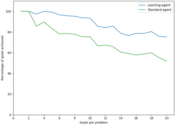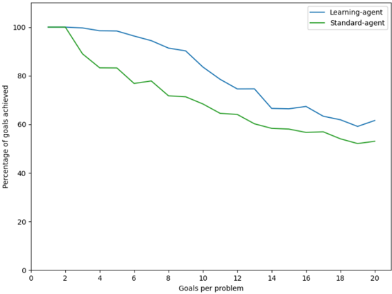## 4.3 Empirical Results In Figure 4, the blue line represents the learning agent, and the green line represents the standard agent. From these results, it is clear that the learning agent performs significantly better than the standard agent because a standard agent removes all invasive plants regardless of any plants in adjacent cells. The learning agent outperforms because, after a given number of trials, it improves its use of herbicide. As the spray operator is gradually fixed, the learning agent generates better plans to remove invasive plants while preserving the native ones. 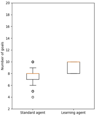For two different points along the x-axis of Figure 4, Figures 5 and 6 show further details using box plots. A box plot is a standardized way of displaying data such as minimum, first quartile, median, third quartile and maximum. The box is drawn from first quartile to third quartile. The lower line below the box is the minimum value (first quartile value -1.5 * interquartile range) and the upper line is the maximum value (first quartile value +1.5 * interquartile range). <details> <summary>Image 4 Details</summary>  ### Visual Description ## Line Chart: Goal Achievement Comparison ### Overview The image is a line chart comparing the percentage of goals achieved by a "Learning-agent" and a "Standard-agent" across a range of "Goals per problem" from 1 to 20. The chart displays the performance of each agent as the number of goals per problem increases. ### Components/Axes * **X-axis:** "Goals per problem", ranging from 0 to 20 in increments of 2. * **Y-axis:** "Percentage of goals achieved", ranging from 0 to 100 in increments of 20. * **Legend (Top-Right):** * Blue line: "Learning-agent" * Green line: "Standard-agent" ### Detailed Analysis * **Learning-agent (Blue Line):** * Trend: Generally decreasing with some fluctuations. * Data Points: * At 1 goal per problem: Approximately 100% * At 2 goals per problem: Approximately 100% * At 4 goals per problem: Approximately 98% * At 6 goals per problem: Approximately 96% * At 8 goals per problem: Approximately 94% * At 10 goals per problem: Approximately 94% * At 12 goals per problem: Approximately 86% * At 14 goals per problem: Approximately 85% * At 16 goals per problem: Approximately 78% * At 18 goals per problem: Approximately 80% * At 20 goals per problem: Approximately 76% * **Standard-agent (Green Line):** * Trend: Decreasing. * Data Points: * At 1 goal per problem: Approximately 100% * At 2 goals per problem: Approximately 100% * At 4 goals per problem: Approximately 86% * At 6 goals per problem: Approximately 80% * At 8 goals per problem: Approximately 78% * At 10 goals per problem: Approximately 78% * At 12 goals per problem: Approximately 66% * At 14 goals per problem: Approximately 64% * At 16 goals per problem: Approximately 60% * At 18 goals per problem: Approximately 58% * At 20 goals per problem: Approximately 52% ### Key Observations * Both agents start with 100% goal achievement at 1 and 2 goals per problem. * The Learning-agent consistently outperforms the Standard-agent across all goal counts. * The performance of both agents decreases as the number of goals per problem increases. * The Standard-agent experiences a more significant drop in performance compared to the Learning-agent. ### Interpretation The chart suggests that the "Learning-agent" is more effective at achieving goals as the complexity of the problem (number of goals per problem) increases. The "Standard-agent" shows a more pronounced decline in performance, indicating it may not adapt as well to more complex scenarios. The data implies that the learning mechanisms implemented in the "Learning-agent" provide a performance advantage over the "Standard-agent," especially when dealing with a higher number of goals per problem. </details> Figure 4 . Experiment 1 performance as a function of problem complexity. The ratio of native to invasive plants is 75:25 in each of the 2,000 trials. As problems increase in complexity given ever more goals to achieve, performance decreases as a percentage of goals achieved. But, the metacognitive agent that learns a better action model outperforms a standard planning agent that uses no metacognition or learning. Figure 5 . Experiment 1 box plots for standard and learning agents in 10-goal problems. <details> <summary>Image 5 Details</summary>  ### Visual Description ## Box Plot: Number of Goals Achieved by Standard and Learning Agents ### Overview The image is a box plot comparing the number of goals achieved by a "Standard agent" and a "Learning agent." The plot visually represents the distribution of goals achieved by each agent type, including the median, quartiles, and outliers. ### Components/Axes * **X-axis:** Categorical axis with two categories: "Standard agent" and "Learning agent." * **Y-axis:** Numerical axis labeled "Number of goals," ranging from 2 to 20, with increments of 2. * **Box Plots:** Each box plot represents the distribution of goals for each agent type. The box represents the interquartile range (IQR), the line inside the box represents the median, and the whiskers extend to the furthest data point within 1.5 times the IQR. Points outside the whiskers are considered outliers. ### Detailed Analysis * **Standard agent:** * The box extends from approximately 7 to 8 goals. * The median is approximately 7.5 goals. * The whiskers extend from approximately 6 to 9 goals. * There are two outliers, one at approximately 4 goals and another at 10 goals. * **Learning agent:** * The box extends from approximately 8 to 10 goals. * The median is approximately 9 goals. * There are no visible whiskers or outliers. ### Key Observations * The Learning agent has a higher median number of goals achieved compared to the Standard agent. * The distribution of goals for the Learning agent appears to be more concentrated, with no visible outliers. * The Standard agent has a wider distribution of goals and includes outliers, suggesting more variability in its performance. ### Interpretation The box plot suggests that the Learning agent is more effective at achieving goals compared to the Standard agent. The higher median and lack of outliers indicate that the Learning agent consistently achieves a higher number of goals. The Standard agent's performance is more variable, with some instances of achieving significantly fewer or more goals than the typical range. This could be due to the Learning agent adapting and improving its performance over time, while the Standard agent's performance remains relatively constant. 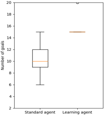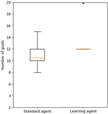</details> Figure 6 . Experiment 1 box plots for standard and learning agents in 20-goal problems. <details> <summary>Image 6 Details</summary>  ### Visual Description ## Box Plot: Number of Goals Achieved by Standard Agent vs. Learning Agent ### Overview The image is a box plot comparing the number of goals achieved by a "Standard agent" and a "Learning agent." The plot visualizes the distribution of goals achieved by each agent, showing the median, quartiles, and outliers. ### Components/Axes * **X-axis:** Agent type (categorical): "Standard agent" and "Learning agent". * **Y-axis:** Number of goals (numerical), ranging from 2 to 20, with tick marks at intervals of 2. * **Box Plot Components:** Each box plot shows the median (orange line), the interquartile range (IQR, the box), and the whiskers extending to the furthest data point within 1.5 times the IQR. Outliers are shown as individual points. ### Detailed Analysis * **Standard Agent:** * The box extends from approximately 9 goals to 12 goals. * The median (orange line) is at approximately 10 goals. * The lower whisker extends down to approximately 6 goals. * The upper whisker extends up to approximately 15 goals. * **Learning Agent:** * The box is a single line at approximately 15 goals, indicating a very narrow interquartile range. * The median (orange line) is at approximately 15 goals. * There is one outlier at approximately 20 goals. ### Key Observations * The learning agent consistently achieves a higher number of goals compared to the standard agent. * The learning agent's performance is much less variable than the standard agent's, as indicated by the narrow box plot. * The learning agent has one outlier, indicating a single instance of exceptionally high performance. ### Interpretation The box plot suggests that the learning agent is significantly more effective at achieving goals than the standard agent. The learning agent's consistent performance, as indicated by the narrow box plot, suggests that it is more reliable. The outlier for the learning agent indicates that it is also capable of achieving exceptionally high performance in some instances. The standard agent's performance is more variable, suggesting that its success is more dependent on external factors or random chance. </details> ## COMPUTATIONAL METACOGNITION In Figures 5 and 6, the orange line represents the median of the distribution. Note that the y-axis reports the number of goals achieved instead of the percentage of goals achieved as in Figure 4. The black circles represent the outliers for the distribution of the data. In Figure 5, it is clear that the median of the standard agent is much less than the median of the learning agent. In Figure 6, the median of the learning agent is significantly greater than the median of the standard agent, and the variance is very low in contrast to the standard agent. By the time 20-goal problems are introduced, the learning agent has learned a complete operator. However, many cases will exist where goals cannot be achieved even with a perfect action model, so performance is less than 20 achievements out of 20 goals. For instance, consider again the example in Figure 3. Because herbicide cannot be sprayed outside the garden itself (e.g., at location (3,1)), the invasive at (3,2) cannot be killed without also killing the native plant. 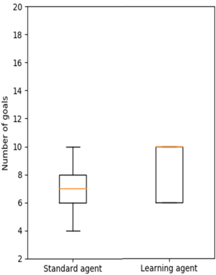In a second experiment with a 60:40 ratio of native to invasive plants, the learning agent still outperforms the standard agent but with less differences in performance (see Figure 7). The reason for this reduced outcome is that fewer examples of native plants being adjacent to invasive ones randomly occur within a 60:40 mix. Box plots are shown in Figures 8 and 9 to provide further details about the variance and significance of the results. ## 5. Related Research As mentioned, computational metacognition has many interpretations in the literature. The cognitive psychology literature includes judgements of learning, feelings of knowing, tip of the tongue states and metamemory phenomena (Dunlosky & Thiede, 2013). But in some work, the definition is so broad as to blur the distinction between cognition and metacognition. For example, Kralik et al. (2018) defines metacognition as any decision process that takes input or output from another decision process. As such, they include planning as a metacognitive process as well as supervisory and arbitration processes. However, to argue that planning and simulation is metacognitive stretches the use of the term and provides little apparent value. The recent work on computational approaches to metacognition are surprisingly thin. Most are either older papers or focus on human psychology rather than artificial intelligence. There is a paper on metacognition applied to neural networks (Babu & Suresh, 2012) and another applied to machine learning (Loeckx, 2017). Neither of these concern high-level reasoning and cognitive systems. Similar to introspective monitoring and meta-level control, the Artificial Cognitive Neural Framework of Crowder, Friess, & Ncc (2011) splits computational metacognition into metacognitive experiences and metacognitive regulation. However, they also add a third component they call metacognitive knowledge or what a cognitive system knows about itself as a cognitive processor. The details of this framework are mainly conceptual, however, and no evaluation exists. A few examples of metareasoning exist in the cognitive systems community such as the work of Martie, Alam, Zhang, & Anderson (2019). Their work on symbolic mirroring learns associations between neural network image classifiers and symbolic abstractions. They use meta-points to reflect on executed and unexecuted sections of the cognitive system itself by passing them to higher-level processes termed meta-operations. Although like MIDCA, the meta-operations examine and modify lower-level processes and involve explanation, much of the work is specific to vision tasks and less general. <details> <summary>Image 7 Details</summary>  ### Visual Description ## Line Chart: Goal Achievement Comparison ### Overview The image is a line chart comparing the percentage of goals achieved by a "Learning-agent" and a "Standard-agent" across a range of goals per problem. The x-axis represents the number of goals per problem, ranging from 0 to 20. The y-axis represents the percentage of goals achieved, ranging from 0 to 100. ### Components/Axes * **X-axis:** "Goals per problem", ranging from 0 to 20 in increments of 2. * **Y-axis:** "Percentage of goals achieved", ranging from 0 to 100 in increments of 20. * **Legend:** Located in the top-right corner. * "Learning-agent" (blue line) * "Standard-agent" (green line) ### Detailed Analysis * **Learning-agent (blue line):** * Trend: Generally decreasing as the number of goals per problem increases. * Data Points: * At 2 goals per problem, approximately 100% achieved. * At 4 goals per problem, approximately 99% achieved. * At 6 goals per problem, approximately 98% achieved. * At 8 goals per problem, approximately 94% achieved. * At 10 goals per problem, approximately 92% achieved. * At 12 goals per problem, approximately 90% achieved. * At 14 goals per problem, approximately 82% achieved. * At 16 goals per problem, approximately 75% achieved. * At 18 goals per problem, approximately 65% achieved. * At 20 goals per problem, approximately 60% achieved. * **Standard-agent (green line):** * Trend: Generally decreasing as the number of goals per problem increases. * Data Points: * At 2 goals per problem, approximately 100% achieved. * At 4 goals per problem, approximately 85% achieved. * At 6 goals per problem, approximately 83% achieved. * At 8 goals per problem, approximately 78% achieved. * At 10 goals per problem, approximately 73% achieved. * At 12 goals per problem, approximately 70% achieved. * At 14 goals per problem, approximately 65% achieved. * At 16 goals per problem, approximately 62% achieved. * At 18 goals per problem, approximately 58% achieved. * At 20 goals per problem, approximately 53% achieved. ### Key Observations * Both agents start at 100% goal achievement for 2 goals per problem. * The Learning-agent consistently outperforms the Standard-agent across all goal-per-problem values greater than 2. * The performance gap between the two agents appears to widen as the number of goals per problem increases. * Both agents experience a decrease in performance as the number of goals per problem increases, indicating that more complex problems are harder to solve. ### Interpretation The data suggests that the "Learning-agent" is more effective at achieving goals in complex problems (higher number of goals per problem) compared to the "Standard-agent". The decreasing trend in both agents' performance indicates that the difficulty of the problems increases with the number of goals. The Learning-agent's ability to maintain a higher percentage of goals achieved suggests it has a better capacity to adapt and solve more complex problems. The widening gap between the two agents as the problem complexity increases highlights the advantage of the learning-based approach. </details> Figure 7. Experiment 2 performance as a function of problem complexity. The ratio of native to invasive plants is 60:40 in each of the 2,000 trials. As problems increase in complexity given ever more goals to achieve, performance goes down in terms of the percentage of goals achieved. Figure 8. Experiment 2 box plots for standard and learning agents in 10-goal problems. <details> <summary>Image 8 Details</summary>  ### Visual Description ## Box Plot: Number of Goals Achieved by Standard and Learning Agents ### Overview The image is a box plot comparing the number of goals achieved by a "Standard agent" and a "Learning agent." The plot displays the distribution of goals achieved by each agent, showing the median, quartiles, and range. ### Components/Axes * **X-axis:** Categorical axis with two categories: "Standard agent" and "Learning agent." * **Y-axis:** Numerical axis labeled "Number of goals," ranging from 2 to 20, with tick marks at intervals of 2. * **Box Plots:** Each box plot represents the distribution of goals for each agent type. The box represents the interquartile range (IQR), the line inside the box represents the median, and the whiskers extend to the minimum and maximum values within 1.5 times the IQR. ### Detailed Analysis * **Standard agent:** * Minimum number of goals: Approximately 4 * First quartile (Q1): Approximately 6 * Median: Approximately 7 * Third quartile (Q3): Approximately 8 * Maximum number of goals: Approximately 10 * **Learning agent:** * Minimum number of goals: Approximately 6 * First quartile (Q1): Approximately 6 * Median: Approximately 8 * Third quartile (Q3): Approximately 10 * Maximum number of goals: Approximately 10 ### Key Observations * The Learning agent has a higher median number of goals achieved compared to the Standard agent. * The range of goals achieved by the Learning agent is smaller than that of the Standard agent. * The interquartile range (IQR) for the Learning agent is higher than the Standard agent. ### Interpretation The box plot suggests that the Learning agent tends to achieve a higher number of goals compared to the Standard agent. The smaller range for the Learning agent indicates more consistent performance. The higher IQR for the Learning agent suggests that the middle 50% of the data is more spread out than the Standard agent. Overall, the Learning agent appears to be more effective in achieving goals. </details> Figure 9. Experiment 2 box plots for standard and learning agents in 20-goal problems. <details> <summary>Image 9 Details</summary>  ### Visual Description ## Box Plot: Number of Goals Achieved by Standard and Learning Agents ### Overview The image is a box plot comparing the number of goals achieved by a "Standard agent" and a "Learning agent." The plot displays the distribution of goals for each agent type, showing the median, quartiles, and outliers. ### Components/Axes * **X-axis:** Categorical axis with two categories: "Standard agent" and "Learning agent." * **Y-axis:** Numerical axis labeled "Number of goals," ranging from 2 to 20, with tick marks at intervals of 2. * **Box Plots:** Each box plot represents the distribution of goals for each agent type. The box represents the interquartile range (IQR), the line inside the box represents the median, and the whiskers extend to the minimum and maximum values within 1.5 times the IQR. Outliers are plotted as individual points. ### Detailed Analysis * **Standard agent:** * The box extends from approximately 10 to 12 goals. * The median (orange line within the box) is approximately 10.5 goals. * The lower whisker extends to approximately 8 goals. * The upper whisker extends to approximately 15 goals. * **Learning agent:** * The median (orange line) is approximately 12 goals. * There is one outlier at approximately 19.8 goals. ### Key Observations * The "Learning agent" has a higher median number of goals achieved compared to the "Standard agent." * The "Learning agent" has an outlier, indicating at least one instance where it achieved a significantly higher number of goals. * The "Standard agent" has a wider distribution of goals, as indicated by the longer whiskers. ### Interpretation The box plot suggests that the "Learning agent" generally performs better than the "Standard agent" in terms of the number of goals achieved. The higher median and the presence of an outlier indicate that the "Learning agent" is capable of achieving a higher number of goals in some instances. The wider distribution of goals for the "Standard agent" suggests that its performance is more variable. </details> ## COMPUTATIONAL METACOGNITION Human metacognition has been studied in the field of cognitive architectures: notably in ACT-R (Anderson, 2009; Larue, Hough, & Juvina, 2018), CLARION (Sun, 2016), and LIDA (Franklin et al., 2007). In ACT-R, Anderson and Fincham (2014) explored how reflective functions supported by metacognition can consciously assesses what one knows and how to extend it to solve a problem. More specifically, metacognition enabled the architecture to reflect on declarative representations of cognitive procedures, allowing for the modification or replacement of elements in the procedures used in mathematical problem-solving. More recent work explored metacognitive trigger mechanisms and more particularly the feeling of rightness (Wang & Thompson, 2019) metacognitive experience, and more particularly how feeling of rightness determines the depth of inner simulation of possible scenarios and hypothesis testing. Metacognition is a key element of CLARION's hybrid (i.e., symbolic and subsymbolic) architecture. Following Flavell's (1976) original definition of metacognition, it supports the active monitoring and regulation of cognitive processes. Metacognitive mechanisms determine how much symbolic and sub-symbolic processing will be involved in decision making and can also dynamically change the ratio of symbolic and sub-symbolic processing and how they interact (e.g., which learning method(s) or reasoning mechanism(s) to apply). Internal parameters (e.g., learning rates, thresholds, and utilities) are also modified through metacognition. In contrast to CLARION and MIDCA, LIDA has no specific metacognitive module. Higherlevel cognitive processes are implemented as collections of behavior streams. Metacognitive processes specifically are a collection of behavior streams (i.e., sequences of actions) that control deliberation through internal actions (e.g., strategy regulation, resource allocation, and the interruption of strategies that have persisted too long in favor of an alternative). We have described metacognition as a kind of add-on to a cognitive system and implemented it as a separate software module in MIDCA. Yet this is not necessarily required computationally. Indeed, metacognition may be a self-reflective aspect of cognition itself. Only further research will clarify the implications of one approach as opposed to the other. ## 6. Conclusion This paper briefly sketches a theory of computational metacognition analogous to a cognitive action-perception cycle and illustrates how it can be implemented in a cognitive architecture. We divide metacognition into three categories: explanatory, immediate and anticipatory metacognition. We discuss the first category in detail and briefly explain the last. Immediate metacognition remains for future research. Finally, we provide an empirical evaluation of explanatory metacognition and show how it improves system performance by progressively learning better action models. Previous publications (Cox & Dannenhauer, 2016; Cox, et al., 2017; Dannenhauer, et al., 2018) report similar results in alternative domains and therefore support the generality of the approach. However, this work is the first time the full metacognitive cycle in MIDCA has been described and demonstrated. Earlier publications focus on specific portions of the meta-level process such as the detection of metacognitive expectation failures, and they make large assumptions about other aspects of the meta-level computation. Yet numerous limitations still exist with respect to the implementation and the theory. As the introduction admits, metacognition is not always the best choice for an agent or for humans. For example, if a system is under severe time constraints, reasoning about reasoning may waste valuable computational resources better spent on cognitive-level problem-solving or action execution. Although future research will provide a greater understanding of the trade-offs involved (see Norman, 2020, for some interesting heuristics that can potentially mitigate this problem), this paper clearly illustrates the positive effect computational metacognition can offer advanced cognitive systems. Furthermore, some of the assumptions in this work remain implicit and underexplored. Although (in machines) statistical reinforcement learning (Sutton & Barto, 1999) or (in humans) operant conditioning (Skinner, 1938, 1957) may be at play at the lower levels of cognition, we view deliberate, goal-driven learning (Cox & Ram, 1999; Ram & Leake, 1995a) as a metacognitive activity. The agent needs to consider why reasoning fails and make decisions to achieve explicit goals to learn and hence (indirectly) improve performance. This perspective conflicts with standard formulations of the learning problem (e.g., Mitchell, 1997) even within the cognitive systems community (e.g., Langley, 2021; Mohan & Laird, 2014). As such, this makes the comparison to and contrast with other learning approaches difficult. Thus, an empirical comparison between an agent that learns with metacognition and one that learns without metacognition is problematic from our point of view. Again, future research will attempt to elaborate upon and evaluate this position and to clarify other assumptions less obvious in this paper. Finally, as the examples shown here demonstrate, MIDCA implements relatively simple solutions for the problem of realizing computational metacognition. At this time, MIDCA's metalevel manages only singleton goal sets, and meta-level plans are currently very short and basic. Interactions between multiple meta-level goals and complex planning alternatives also remain for future work. But previous results shown at the cognitive level with MIDCA together with the robust state of the art in the planning community suggest that solutions to more complicated problems at the meta-level will be relatively straight forward and within practical reach. Rather than focus on sophisticated problems sets that rarely occur, we have instead put forth a fundamental approach to metacognition that promises to change the way we think about what makes a cognitive system intelligent and learning effective. ## Acknowledgements This research is supported in part by the National Science Foundation through grant S&AS1849131 and by the Office of Naval Research (ONR) through grant N00014-18-1-2009. We also thank the anonymous reviewers for their comments, insights, and suggestions and Matt Molineaux for suggesting the use of FOIL as a learning mechanism and his overall technical critique. Finally, we gratefully thank Paul Bello (a previous program manager at ONR) for taking a risk and funding the MIDCA project when it was merely a proposed concept ten years ago. ## References - Aha, D. W. (2018). Goal reasoning: Foundations, emerging applications, and prospects. AI Magazine, 39, 3-24. - Amos-Binks, A., Dannenhauer, D. (2019). Anticipatory thinking: A metacognitive capability. In Working Notes of the 7th Goal Reasoning Workshop . Cambridge, MA. Advances in Cognitive Systems 2019. ## COMPUTATIONAL METACOGNITION - Anderson, J. R. (2009). How can the human mind occur in the physical universe? Oxford, UK: Oxford University Press. - Anderson, J. R., & Fincham, J.M. (2014). Extending problem-solving procedures through reflection. Cognitive psychology 74, 1-34. - Babu, G., & Suresh, S. (2012). Meta-cognitive neural network for classification problems in a sequential learning framework. Neurocomputing 81. 86-96. 10.1016/j.neucom.2011.12.001. - Boggs, J., Dannenhauer, D., Floyd, M. W., & Aha, D. W. (2018). The ideal rebellion: Maximizing task performance in rebel agents. In Proceedings of the 6th Goal Reasoning Workshop , held at IJCAI/FAIM-2018. - Brown, A. (1987). Metacognition, executive control, self-regulation, and other more mysterious mechanisms. In F. E. Weinert & R. H. Kluwe (Eds.), Metacognition, motivation, and understanding (pp. 65-116). Hillsdale, NJ: Lawrence Erlbaum Associates. - Conitzer, V. (2011). Metareasoning as a formal computational problem. In M. T. Cox & A. Raja (Eds.) Metareasoning: Thinking about thinking (pp. 121-127). Cambridge, MA: MIT Press. - Cox, M. T. (1997). Loose coupling of failure explanation and repair: Using learning goals to sequence learning methods. In D. B. Leake & E. Plaza (Eds.), Case-Based Reasoning Research and Development: Second International Conference on Case-Based Reasoning (pp. 425-434). Berlin: Springer-Verlag. - Cox, M. T. (2005). Metacognition in computation: A selected research review. Artificial Intelligence 169(2), 104-141. - Cox, M. T. (2011). Metareasoning, monitoring, and self-explanation. In M. T. Cox & A. Raja (Eds.) Metareasoning: Thinking about thinking (pp. 131-149). Cambridge, MA: MIT Press. - Cox, M. T. (2020). The problem with problems. In Proceedings of the Eighth Annual Conference on Advances in Cognitive Systems . Palo Alto, CA: Cognitive Systems Foundation. - Cox, M. T., Alavi, Z., Dannenhauer, D., Eyorokon, V., Munoz-Avila, H., & Perlis, D. (2016). MIDCA: A metacognitive, integrated dual cycle architecture for self regulated autonomy. In Proceedings of the Thirtieth AAAI Conference on Artificial Intelligence , Vol. 5 (pp. 3712-3718). Palo Alto, CA: AAAI Press. - Cox, M. T., & Dannenhauer, D. (2016). Goal transformation and goal reasoning. In Proceedings of the 4 th Workshop on Goal Reasoning . New York, IJCAI-16. - Cox, M. T., & Dannenhauer, Z. A. (2017). Perceptual goal monitors for cognitive agents in changing environments. In Proceedings of the Fifth Annual Conference on Advances in Cognitive Systems, Poster Collection (pp. 1-16). Palo Alto, CA: Cognitive Systems Foundation. - Cox, M. T., Dannenhauer, D., & Kondrakunta, S. (2017). Goal operations for cognitive systems. In Proceedings of the Thirty-first AAAI Conference on Artificial Intelligence (pp. 4385-4391). Palo Alto, CA: AAAI Press. - Cox, M. T., Oates, T., & Perlis, D. (2011). Toward an integrated metacognitive architecture. In P. Langley (Ed.), Advances in Cognitive Systems: Papers from the 2011 AAAI Fall Symposium (pp. 74-81). Technical Report FS-11-01. Menlo Park, CA: AAAI Press. - Cox, M. T., & Ram, A. (1999). Introspective multistrategy learning: On the construction of learning strategies. Artificial Intelligence, 112, 1-55. - Cox, M. T., & Veloso, M. M. (1998). Goal transformations in continuous planning. In M. desJardins (Ed.), Proceedings of the 1998 AAAI Fall Symposium on Distributed Continual Planning (pp. 23-30). Menlo Park, CA: AAAI Press / The MIT Press. - Crowder, J., Friess, S., & Ncc, M. (2011). Metacognition and metamemory concepts for AI systems. In Proceedings of the 2011 World Congress in Computer Science, Computer Engineering, & Applied Computing: The 2011 International Conference on Artificial Intelligence . CSREA Press. - Dannenhauer, D., Cox, M. T., & Munoz-Avila, H. (2018). Declarative metacognitive expectations for high-level cognition. Advances in Cognitive Systems , 6, 231-250. - Dannenhauer, D., & Munoz-Avila, H. (2015). Raising expectations in GDA agents acting in dynamic environments. In Proceedings of the Twenty-Fourth International Joint Conference on Artificial Intelligence (pp. 2241-2247). Menlo Park, CA: AAAI Press. - Dunlosky, J., & Thiede, K. W. (2013). Metamemory. In D. Reisberg (Ed.), The Oxford handbook of cognitive psychology (pp. 283-298). Oxford, UK: Oxford University Press. - Edelkamp, S., & Hoffmann, J. (2004). PDDL2.2: The language for the classical part of the 4th international planning competition . Technical Report 195, University of Freiburg. - Flavell, J. H. (1976). Metacognitive aspects of problem solving. In A. Resnick (Ed.), The nature of intelligence (pp. 231-235). Hillsdale, NJ: LEA. - Franklin, S., Ramamurthy, U., D'Mello, S., McCauley, L., Negatu, A., Silva R., & Datla, V. (2007). LIDA: A computational model of global workspace theory and developmental learning. In AAAI Fall Symposium on AI and Consciousness: Theoretical Foundations and Current Approaches . Menlo Park, CA: AAAI Press. - Ghallab, M., Nau, D., & Traverso, P. (2004). Automated planning: Theory and practice . San Francisco: Morgan Kaufmann. - Gogineni, V. R., Kondrakunta, S., & Cox, M. T. (in press). Multi-agent goal delegation. To appear in Proceedings of the 9 th Goal Reasoning Workshop . Advances in Cognitive Systems 2021. - Gogineni, V. R., Kondrakunta, S., Molineaux, M., & Cox, M. T. (2018). Application of case-based explanations to formulate goals in a unpredictable mine clearance domain. In M. Minor (Ed.), 26th International Conference on Case-Based Reasoning: Workshop Proceedings - Case-based Reasoning for the Explanation of Intelligent Systems (pp. 42-51). ICCBR-18. - Goldman, A. I. (2006). Simulating minds . Oxford, UK: Oxford University Press. - Gopnik, A. (2012). Reconstructing constructivism: Causal models, Bayesian learning mechanisms, and the theory theory. Psychological Bulletin, 138 (6), 1085-1108. - Hayes-Roth, F., Waterman, D. A., & Lenat, D. B. (Eds.) (1983). Building Expert Systems . London: Addison-Wesley. - Helmert, M. (2006). The fast downward planning system. Journal of Artificial Intelligence Research , 26, 191-246. - Helmert, M., Röger, G., & Karpas, E. (2011). Fast downward stone soup: A baseline for building planner portfolios. In ICAPS 2011 Workshop on Planning and Learning (pp. 28-35). - Horvitz, E. J. (1990). Rational metareasoning and compilation for optimizing decisions under bounded resources . Knowledge Systems Laboratory, Medical Computer Science, Stanford University. ## COMPUTATIONAL METACOGNITION - Kondrakunta, S. (2017). Implementation and evaluation of goal selection in a cognitive architecture . Master's thesis, Wright State University, College of Engineering and Computer Science, Dayton, OH. - Kondrakunta, S., & Cox, M. T. (in press). Autonomous goal selection operation for agent based architectures. To appear in Proceedings of the 2021 World Congress in Computer Science, Computer Engineering, & Applied Computing (CSCE'21). - Kondrakunta, S., Gogineni, V. R., & Cox, M. T. (in press). Agent goal management using goal operations. To appear in Proceedings of the 9 th Goal Reasoning Workshop . Advances in Cognitive Systems 2021. - Kralik, J. D., Lee, J. H., Rosenbloom, P. S., Jackson, P. C., Epstein, S. L., Romero, O. J., Sanz, R., Larue, O., Schmidtke, H. R., Lee, S. W., & McGreggor, K. (2018). Metacognition for a common model of cognition. Procedia Computer Science , 145, 730-739. - Mohan, S., & Laird J. E. (2014). Learning goal-oriented hierarchical tasks from situated interactive instruction. Proceedings of the 28th AAAI Conference on Artificial Intelligence. Menlo Park, CA: AAAI Press. - Langley, P. (2017). A cognitive systems analysis of personality and conversational style. Advances in Cognitive Systems , 5, 1-12. - Langley, P. (2021). The computational gauntlet of human-like learning . Manuscript submitted for publication. - Larue, O., Hough, A., & Juvina, I. (2018). A cognitive model of switching between reflective and reactive decision making in the Wason task. In I. Juvina, J. Houpt, and C. Myers (Eds.) Proceedings of the Sixteenth International Conference on Cognitive Modeling (pp. 55-60). Madison, WI: University of Wisconsin. - Loeckx, J. (2017). The case for meta-cognitive machine learning: On model entropy and concept formation in deep learning. ArXiv , abs/1711.01431. - Martie, L., Alam, A., Zhang, G., & Anderson, R. (2019). Reflecting after learning for understanding. Advances in Cognitive Systems 8, 53-7. - Mitchell, T. M. (1997). Machine learning . New York: McGraw-Hill. - Mohammad, Z. (2021). A rebellion framework with learning for goal-driven autonomy . Master's dissertation, Wright State University, Department of Computer Science and Engineering, Dayton, OH. - Mohammad, Z., Cox, M. T., & Molineaux, M. (2020). Rebel agents that learn from plan execution failures. In Proceedings of the Integrated Execution / Goal Reasoning Workshop (held at the Thirtieth International Conference on Automated Planning and Scheduling - ICAPS-20), Nancy, France. - Munoz-Avila, H. (2018). Adaptive goal driven autonomy. In Cox, M. T., Funk, P., & Begum, S. (Eds.) (2018). Case-Based Reasoning Research and Development: Proceedings of the 26th International Conference (pp. 3-12). Berlin: Springer. - Munoz-Avila, H., & Cox, M. T. (2008). Case-based plan adaptation: An analysis and review . IEEE Intelligent Systems, 23(4), 75-81. - Norman, E. (2020). Metacognition is not always helpful. Frontiers in Psychology , 11, 15-37. - Paisner, M., Cox, M. T., Maynord, M., & Perlis, D. (2014). Goal-driven autonomy for cognitive systems. In Proceedings of the 36th Annual Conference of the Cognitive Science Society (pp. 2085-2090). Austin, TX: Cognitive Science Society. - Pettersson, O. (2005). Execution monitoring in robotics: A survey. Robotics and Autonomous Systems , 53, 73-88. - Price, J., Hertzog, C., & Dunlosky, J. (2009). Self-regulated learning in younger and older adults: Does aging affect metacognitive control?. Neuropsychology, development, and cognition. Section B, Aging, neuropsychology and cognition, 17, 329-59. - Quinlan, J. R. (1990). Learning logical definitions from relations. Machine learning , 5(3), 239-266. - Ram, A., & Cox, M. T. (1994). Introspective reasoning using meta-explanations for multistrategy learning. In R. S. Michalski & G. Tecuci (Eds.), Machine learning: A multistrategy approach IV (pp. 349-377). San Francisco: Morgan Kaufmann. - Ram, A., & Leake, D. (1995a). Goal-driven learning . Cambridge, MA: MIT Press. - Ram, A., & Leake, D. (1995b). Learning, goals, and learning goals. In A. Ram & D. Leake (Eds.), Goal-driven learning (pp. 1-37). Cambridge, MA: MIT Press/Bradford Books. - Reder, L. M., & Ritter, F. (1992). What determines initial feeling of knowing? Familiarity with question terms, not with the answer, Journal of Experimental Psychology , 18(3) 435-451. - Roberts, M., Borrajo, D., Cox, M. T., & Yorke-Smith, N. (Eds.) (2018). Special issue on goal reasoning. AI Communications , 31(2), 115-116. - Schank, R. C. (1982). Dynamic memory: A theory of reminding and learning in computers and people . Cambridge, MA: Cambridge University Press. - Schank, R. C. (1986). Explanation patterns: Understanding mechanically and creatively . Hillsdale, NJ: Lawrence Erlbaum. - Schank, R. C., & Owens, C. C. (1987). Understanding by explaining expectation failures. In R. G. Reilly (Ed.), Communication failure in dialogue and discourse . New York: Elsevier Science. - Searle, J. R. (1969). Speech acts: An essay in the philosophy of language . Cambridge, UK: Cambridge University Press. - Skinner, B. F. (1938). The behavior of organisms: An experimental analysis . New York: AppletonCentury-Crofts. - Skinner, B. F. (1957). Verbal behavior . New York: Appleton-Century-Crofts. - Sun, R. (2016). Anatomy of the mind: Exploring psychological mechanisms and processes with the Clarion cognitive architecture . Oxford, UK: Oxford University Press. - Sutton, R. S., & Barto, A. G. (1999). Reinforcement learning. Journal of Cognitive Neuroscience , 11(1), 126-134. - Wang, S., & Thompson, V. (2019). Fluency and feeling of rightness: The effect of anchoring and models. Psychological Topics , 28, 37-72. - Wellman, H. M. (1990). The child's theory of mind . Cambridge, MA: MIT Press. - Wilson, T. D., & Schooler, J. W. (1991). Thinking too much: Introspection can reduce the quality of preferences and decisions. Journal of Personality and Social Psychology , 60(2), 181-192. - Zilberstein, S. (2011). Metareasoning and bounded rationality. In M. T. Cox & A. Raja (Eds.) Metareasoning: Thinking about thinking (pp. 27-40). Cambridge, MA: MIT Press.