2202.02891

## Causal Inference Using Tractable Circuits ## Adnan Darwiche Computer Science Department University of California, Los Angeles darwiche@cs.ucla.edu ## Abstract The aim of this paper is to discuss a recent result which shows that probabilistic inference in the presence of (unknown) causal mechanisms can be tractable for models that have traditionally been viewed as intractable. This result was reported recently in [15] to facilitate model-based supervised learning but it can be interpreted in a causality context as follows. One can compile a non-parametric causal graph into an arithmetic circuit that supports inference in time linear in the circuit size. The circuit is also non-parametric so it can be used to estimate parameters from data and to further reason (in linear time) about the causal graph parametrized by these estimates. Moreover, the circuit size can sometimes be bounded even when the treewidth of the causal graph is not, leading to tractable inference on models that have been deemed intractable previously. This has been enabled by a new technique that can exploit causal mechanisms computationally but without needing to know their identities (the classical setup in causal inference). Our goal is to provide a causality-oriented exposure to these new results and to speculate on how they may potentially contribute to more scalable and versatile causal inference. ## 1 Introduction Tractable arithmetic circuits have been receiving an increased attention in AI and computer science more broadly; see [16] for a recent survey. These circuits represent real-valued functions and are called tractable because they allow one to answer some hard queries about these functions through linear-time, feed-forward passes on the circuit structure. These circuits were initially compiled from Bayesian networks as proposed in [13, 12] to facilitate probabilistic reasoning. They were later learned from data, starting with [23], and even handcrafted as initially proposed in [30]. Traditional methods for exact probabilistic inference have a complexity which is exponential in treewidth (a graph-theoretic parameter that measures the model's connectivity). With the introduction of compiled circuits, one could practically do inference on models whose treewidth can be in the hundreds; see, e.g., [5, 8, 7]. A recent comprehensive, empirical evaluation of at least a dozen probabilistic inference algorithms showed that methods based on circuits are at the forefront in terms of efficiency [1]; see also [18]. What stands behind the efficacy of circuit-based methods is their ability to aggresively exploit the parametric structure of models such as functional dependencies and context-specific independence [4]. This however has limited their utility in contexts where one does not know the model parameters, which is a common case in causal inference. A circuit compilation method was recently proposed in [15] which can exploit a more abstract form of parametric structure: functional dependencies (i.e., causal mechanisms) whose identities are unknown which is the classical setup in causal inference. This new method was able to compile circuits for models whose treewidth is very large without needing to know the model parameters, leading to a major advance on earlier techniques. Our aim in this paper is to provide an intuitive exposure to this new algorithm and its underlying techniques, while placing it in a causality context. Our belief is that a discussion of these new results could lead to a synthesis on how they can further advance causal inference in terms of scalability and versatility. We start first with a review of some core concepts in causality and circuit-based inference and then follow by a discussion of the new results and their significance. ## 2 Causal Models and Queries Variables are discrete and denoted by uppercase letters (e.g., X ) and their values by lowercase letters (e.g., x ). Sets of variables are denoted by boldface, uppercase letters (e.g., X ) and their instantiations by boldface, lowercase letters (e.g., x ). We will write x ∈ x to mean that x is the value of variable X in instantiation x . For a binary variable X , we will use x and ¯ x to denote X =1 and X =0 , respectively. We next define Structural Causal Models (SCMs) following the treatment in [21]; see also [26]. Definition 1. An SCM is a tuple M = ( U , V , F , { Pr ( U ) } U ∈ U ) where U and V are disjoint sets of variables called 'exogenous' and 'endogenous,' respectively; F contains exactly one function f V for each endogenous variable V ; and Pr ( U ) are distributions over exogenous variables U . A function f V is called a 'causal mechanism' and it determines the value of variable V based on two sets of inputs, U V ⊆ U and V V ⊆ V . That is, the mechanism f V is a mapping U V , V V ↦→ V . The causal graph G of an SCM contains variables U ∪ V as its nodes. It also contains edges X → V for each endogenous variable V and each variable X that is an input to function f V . We will only deal with SCMs that produce acyclic causal graphs (the inputs of a function cannot depend on its output). Moreover, we will assume that exogenous variables are independent and that only endogenous variables can be observed. A key observation about SCMs is that once we fix the values of exogenous variables, the values of all endogenous variables are also fixed by the causal mechanisms. 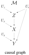We will next consider an example SCM from [2] where all variables are binary. The endogenous variables are V = X,Y,Z , representing a treatment, the outcome and the presence of hypertension, respectively. The exogenous variables are U = U r , U x , U y , U z , representing natural resistance to disease ( U r ) and sources of variation affecting endogenous variables ( U x , U y , U z ). The distributions of exogenous variables are Pr ( u r ) = 0 . 25 , Pr ( u x ) = 0 . 9 , Pr ( u y ) = 0 . 7 and Pr ( u z ) = 0 . 95 . The three causal mechanisms are given next and they lead to the causal graph on the right: <!-- formula-not-decoded --> <details> <summary>Image 1 Details</summary>  ### Visual Description ## Causal Diagram: Directed Acyclic Graph ### Overview The image presents a directed acyclic graph (DAG) representing a causal model. It illustrates the relationships between variables denoted by letters (U, Z, X, Y) and their dependencies, indicated by arrows. The graph includes exogenous variables (U) influencing endogenous variables (Z, X, Y). ### Components/Axes * **Nodes:** Represented by letters: U_z, U_r, Z, U_x, X, U_y, Y. * **Edges:** Represented by arrows, indicating the direction of causal influence. * **Title:** "causal graph" located at the bottom of the diagram. * **Overall Title:** "M" located at the top of the diagram. ### Detailed Analysis The diagram shows the following causal relationships: * U_z influences Z. * U_r influences Z and Y. * U_x influences X. * U_y influences Y. * Z influences X. * X influences Y. The arrows indicate the direction of influence. For example, the arrow from U_z to Z means that U_z has a causal effect on Z. ### Key Observations * Z is influenced by U_z and U_r. * X is influenced by U_x and Z. * Y is influenced by U_y, U_r, and X. * The graph is acyclic, meaning there are no feedback loops. ### Interpretation The causal diagram represents a simplified model of how different variables influence each other. It suggests that Z is a mediator between U_z, U_r and X, and X is a mediator between Z and Y. U_r also has a direct effect on Y. The exogenous variables (U_z, U_r, U_x, U_y) represent unobserved or background factors that influence the endogenous variables (Z, X, Y). The diagram can be used to analyze causal pathways and identify potential interventions to influence the outcome variable Y. 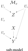</details> A key notion in causal inference is the sub-model M z of an SCM M , where z is an instantiation of some endogenous variables. This is another SCM obtained from M by replacing the function for each variable Z ∈ Z with the constant function f Z = z , where z ∈ z . Intuitively, the sub-model M z is used to reason about an intervention from outside the system modeled by M , which suppresses the causal mechanisms of variables Z and fixes the values of these variables to z . For example, if we intervene to administer a treatment ( x ) in the above SCM M , we get a sub-model M x in which the mechanism for variable X is replaced with the constant function f X = x . The causal graph of the resulting sub-model is shown on the right. sub-model <details> <summary>Image 2 Details</summary>  ### Visual Description ## Diagram: Causal Diagram of a Sub-Model ### Overview The image presents a causal diagram representing a sub-model. It illustrates the relationships between variables X, Y, and Z, along with their respective unobserved confounders U_x, U_y, U_z, and U_r. The diagram shows the causal pathways and dependencies between these variables. ### Components/Axes * **Variables:** X, Y, Z, U_x, U_y, U_z, U_r, M_x * **Arrows:** Represent causal relationships. * **Text:** "sub-model" at the bottom. ### Detailed Analysis * **M_x:** Located at the top of the diagram. * **U_z:** Located at the top-left, with an arrow pointing to Z. * **U_r:** Located at the top-right, with an arrow pointing to Z and Y. * **Z:** Located in the upper-middle, with an arrow pointing to X. * **U_x:** Located to the left of X. * **X:** Located in the middle, with an arrow pointing to Y. * **U_y:** Located to the left of Y, with an arrow pointing to Y. * **Y:** Located at the bottom, representing the outcome variable. * **Arrows:** * U_z -> Z * U_r -> Z * U_r -> Y * Z -> X * U_x -> X * X -> Y * U_y -> Y ### Key Observations * Z is a mediator between U_z, U_r and X. * X is a mediator between Z, U_x and Y. * Y is influenced by X, U_y, and U_r. * U_r is a confounder affecting both Z and Y. ### Interpretation The diagram represents a causal model where X influences Y, and Z influences X. The variables U_x, U_y, U_z, and U_r represent unobserved confounders that may affect the relationships between the observed variables. The presence of U_r influencing both Z and Y indicates a potential confounding effect that needs to be addressed when analyzing the causal relationship between Z and Y. The "sub-model" label suggests that this diagram is a part of a larger causal model. </details> Three types of queries are normally posed on SCMs, which are referred to as associational, interventional and counterfactual queries. They correspond to what is known as the causal hierarchy [26, 28, 27], where each class of queries belongs to a rung [28] or layer [2] in the hierarchy. We next define the syntax and semantics of these queries, using a slightly different notation than is customary-this will allow us to provide a more uniform and general treatment of these queries. Definition 2. An 'observational event' has the form x where X is a set of endogenous variables. An 'interventional event' has the form y x where X and Y are sets of endogenous variables. A 'counterfactual event' has the form η 1 , . . . , η n where η i is an observational or interventional event. An observational event x says that variables X took the value x . For example, a patient did not take the treatment and died ( ¯ x, ¯ y ). An interventional event y x says that variables Y took the value y after setting variables X to x by an intervention. For example, a patient survived after they were given the treatment ( y x ). A counterfactual event is a conjunction of events where each could be observational or interventional. For example, a patient who responds to treatment did not take it and died ( y x , ¯ x, ¯ y ). Definition 3. A 'world' for SCM M is an instantiation of its exogenous variables. The worlds of an observational event W M ( x ) are those worlds that fix the values of variables X to x . The worlds of an interventional event W M ( y x ) are defined as W M x ( y ) . The worlds of a counterfactual event W M ( η 1 , . . . , η n ) are defined as W M ( η 1 ) ∩ . . . ∩ W M ( η n ) . The following table, borrowed from [2], shows all sixteen worlds of the above SCM M , together with their probabilities and the unique states they entail for endogenous variables. | | Ur | Uz | xn | Uy | Z | X | Y | P(u) | | Ur | ²n | xn | Uy | Z | X | Y | P(u) | |----|------|------|------|------|-----|-----|-----|----------|----|------|------|------|------|-----|-----|-----|----------| | 1 | 0 | 0 | 0 | 0 | 0 | 1 | 0 | 0.001125 | 9 | 1 | 0 | 0 | 0 | 0 | 1 | 1 | 0.000375 | | 2 | 0 | 0 | 0 | 1 | 0 | 1 | 0 | 0.002625 | 10 | 1 | 0 | 0 | 1 | 0 | 1 | 1 | 0.000875 | | 3 | 0 | 0 | 1 | 0 | 0 | 0 | 1 | 0.010125 | 11 | 1 | 0 | 1 | 0 | 0 | 0 | 0 | 0.003375 | | 4 | 0 | 0 | 1 | 1 | 0 | 0 | 0 | 0.023625 | 12 | 1 | 0 | 1 | 1 | 0 | 0 | 1 | 0.007875 | | 5 | 0 | 1 | 0 | 0 | 0 | 1 | 0 | 0.021375 | 13 | 1 | 1 | 0 | 0 | 1 | 0 | 0 | 0.007125 | | 6 | 0 | 1 | 0 | 1 | 0 | 1 | 0 | 0.049875 | 14 | 1 | 1 | 0 | 1 | 1 | 0 | 1 | 0.016625 | | 7 | 0 | 1 | 1 | 0 | 0 | 0 | 1 | 0.192375 | 15 | 1 | 1 | 1 | 0 | 1 | 1 | 1 | 0.064125 | | 8 | 0 | 1 | 1 | 1 | 0 | 0 | 0 | 0.448875 | 16 | 1 | 1 | 1 | 1 | 1 | 1 | 1 | 0.149625 | Using this table and a similar one for sub-model M x , we obtain W M (¯ x, ¯ y ) = { u 4 , u 8 , u 11 , u 13 } and W M ( y x ) = { u 9 , . . . , u 16 } which leads to W M ( y x , ¯ x, ¯ y ) = W M (¯ x, ¯ y ) ∩ W M ( y x ) = { u 11 , u 13 } . We are now ready to define the probability of any SCM event. Definition 4. Let M be an SCM with exogenous variables U and distributions Pr ( U ) for U ∈ U . The probability of event η with respect to SCM M is defined as: <!-- formula-not-decoded --> Hence, Pr (¯ x, ¯ y ) = Pr ( u 4 ) + Pr ( u 8 ) + Pr ( u 11 ) + Pr ( u 13 ) = 0 . 4830 and Pr ( y x , ¯ x, ¯ y ) = 0 . 0105 . We can now compute the probability that a patient who did not take the treatment and died would have been alive had they been given the treatment, Pr ( y x | ¯ x, ¯ y ) = Pr ( y x , ¯ x, ¯ y ) / Pr (¯ x, ¯ y ) = 0 . 0217 . We will focus next on associational and interventional queries, leaving counterfactuals to future work. ## 3 Causal Inference Using Circuits As we just saw, one can answer sophisticated causal queries based on a fully specified SCM. However, such a model may not be available, particularly the identities of causal mechanisms and the distributions over exogenous variables. What is more common is to have the causal graph of an underlying SCM in addition to observational data about endogenous variables. A key task of causal inference is then to draw conclusions based on this limited input, particularly about interventional probabilities which is the task we shall focus on. We will next show how this cross-layer inference can be realized using feed-forward circuits that are compiled from the non-parametric causal graphs of SCMs. The discussion will reveal the significance of compiling the smallest possible circuit for a causal graph. It will also motivate the new compilation algorithm in [15] which is particularly relevant to the causal graphs of SCMs (in contrast to Bayesian networks). We shall discuss and study further this algorithm in Sections 4-6 where we will also contribute to understanding its complexity. 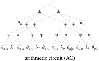The Circuits of Causal Graphs Consider the causal graph X ← U → Y over binary variables and its compiled arithmetic circuit (AC) shown on the right. This circuit has two types of inputs: symbolic parameters θ and indicators λ . There are two parameters for exogenous variable U ( θ u and θ ¯ u ) which specify its distribution. There are four parameters for endogenous variable X ( θ x | u , θ ¯ x | u , θ x | ¯ u , θ ¯ x | ¯ u ) which specify its causal mechanism. The remaining four parameters specify the mechanism for endogenous variable Y . The indicators correspond to the <details> <summary>Image 3 Details</summary>  ### Visual Description ## Arithmetic Circuit Diagram ### Overview The image presents a diagram of an arithmetic circuit (AC). It depicts a hierarchical structure of mathematical operations, specifically additions (+) and multiplications (*), applied to various input variables and parameters. The diagram illustrates the flow of computation from the bottom (inputs) to the top (final result). ### Components/Axes * **Nodes:** The diagram consists of nodes representing mathematical operations (+ and *). * **Inputs:** The bottom layer of the diagram shows the input variables and parameters, denoted as: * θx|u * λx * θx|ū * θx|ū * λx * θx|ū * θy|u * λy * θy|ū * θy|ū * λy * θy|ū * **Intermediate Variables:** Intermediate variables are represented by θu and θū. * **Operations:** The diagram shows alternating layers of multiplication (*) and addition (+) operations. * **Output:** The top node represents the final result of the arithmetic circuit, denoted by a plus sign (+). ### Detailed Analysis The arithmetic circuit diagram is structured as follows: 1. **Bottom Layer (Inputs):** The inputs are arranged linearly at the bottom. 2. **First Layer of Multiplications:** Each pair of adjacent inputs is multiplied. 3. **First Layer of Additions:** The results of the multiplications are added in pairs. 4. **Second Layer of Multiplications:** The results of the additions are multiplied. 5. **Second Layer of Additions:** The results of the multiplications are added. 6. **Top Node (Output):** The final result is obtained at the top node. ### Key Observations * The diagram illustrates a specific arithmetic circuit with a fixed structure. * The circuit involves a combination of multiplication and addition operations. * The inputs consist of variables and parameters related to x, y, u, and ū. ### Interpretation The arithmetic circuit diagram represents a computational process where inputs are combined through a series of multiplications and additions to produce a final result. The specific structure of the circuit determines the mathematical function it computes. The diagram provides a visual representation of the flow of computation and the relationships between different variables and operations. The circuit likely represents a specific mathematical function or algorithm, possibly related to machine learning or signal processing. The parameters θ and λ likely represent weights or coefficients in the computation. </details> values of endogenous variables. Variable X has indicators λ x and λ ¯ x and variable Y has indicators λ y and λ ¯ y . This circuit can compute the probability of any observational event η = x in time linear in the circuit size. We simply set each indicator to 1 if its subscript is compatible with the event η , otherwise we set it to 0 , and then evaluate the circuit [13]. For the event η = ¯ x , the indicators are set to λ x =0 , λ ¯ x =1 , λ y =1 , λ ¯ y =1 . If we (symbolically) evaluate the circuit under this indicator setting, we get θ u θ ¯ x | u ( θ y | u + θ ¯ y | u ) + θ ¯ u θ ¯ x | ¯ u ( θ y | ¯ u + θ ¯ y | ¯ u ) which is the expected result, Pr (¯ x ) . The circuit can also compute the probability of any interventional event η = y x in time linear in the circuit size. This is remarkably simple as well. To compute Pr ( y x ) , known as the causal effect, we first set the parameters of all variables in X to 1 and then evaluate the circuit at instantiation x , y . 1 Suppose that x = ¯ x and y = ¯ y in our running example. To compute Pr (¯ y ¯ x ) , we evaluate the circuit while setting the parameters for variable X to θ x | u = θ ¯ x | u = θ x | ¯ u = θ ¯ x | ¯ u = 1 , and setting the indicators to λ x =0 , λ ¯ x =1 , λ y =0 , λ ¯ y =1 . If we (symbolically) evaluate the circuit under these settings, we get Pr (¯ y ¯ x ) = θ u θ ¯ y | u + θ ¯ u θ ¯ y | ¯ u = Pr (¯ y ) which is the expected result ( X has no causal effect on Y ). Exploiting Unknown Mechanisms Consider the endogenous variable X in the causal graph we just discussed and its parameters θ x | u , θ ¯ x | u , θ x | ¯ u , θ ¯ x | ¯ u . Since these parameters specify a causal mechanism, they must all be in { 0 , 1 } subject to the constraints θ x | u + θ ¯ x | u = 1 and θ x | ¯ u + θ ¯ x | ¯ u = 1 . The main contribution of the new compilation algorithm in [15] is that it can exploit these constraintswithout needing to know the specific values of θ x | u , θ ¯ x | u , θ x | ¯ u , θ ¯ x | ¯ u -to produce circuits whose size can be exponentially smaller compared to methods developed during the last two decades; see, e.g., [13, 5, 6, 11, 32] and [14, Chapters 12,13]. These earlier methods can exploit functional dependencies computationally but only if they know the specific values of parameters. This does not help in a causality context (or a learning context more generally) where we do not know these values. The details of how the algorithm does this are discussed in Sections 4-6. 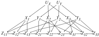For now, consider the family of causal graphs on the right which generally has variables U X , U Y , X i , Y j , Z ij for i, j = 1 , . . . , n . These models have treewidth ≥ n +1 and hence are not accessible to non-parametric inference methods as they take time exponential in n . Moreover, the causal effect of X 1 on Z nn has the only back-door <details> <summary>Image 4 Details</summary>  ### Visual Description ## Diagram: Causal Network ### Overview The image presents a causal network diagram illustrating relationships between variables denoted as U, X, Y, and Z. The diagram shows directed edges (arrows) indicating the direction of influence between these variables. The network is structured in three layers, with U at the top, X and Y in the middle, and Z at the bottom. ### Components/Axes * **Nodes:** The nodes in the diagram represent variables. * Top Layer: U_X, U_Y * Middle Layer: X₁, Y₁, X₂, Y₂, X₃, Y₃ * Bottom Layer: Z₁₁, Z₁₂, Z₁₃, Z₂₁, Z₂₂, Z₂₃, Z₃₁, Z₃₂, Z₃₃ * **Edges:** The edges (arrows) represent causal relationships. The direction of the arrow indicates the direction of influence. ### Detailed Analysis The diagram can be analyzed layer by layer: * **Top Layer (U):** * U_X influences X₁, X₂, and X₃. * U_Y influences Y₁, Y₂, and Y₃. * **Middle Layer (X, Y):** * X₁ influences Z₁₁, Z₁₂, Z₁₃, Z₂₁, Z₂₂, Z₂₃, Z₃₁, Z₃₂, Z₃₃. * Y₁ influences Z₁₁, Z₁₂, Z₁₃, Z₂₁, Z₂₂, Z₂₃, Z₃₁, Z₃₂, Z₃₃. * X₂ influences Z₁₁, Z₁₂, Z₁₃, Z₂₁, Z₂₂, Z₂₃, Z₃₁, Z₃₂, Z₃₃. * Y₂ influences Z₁₁, Z₁₂, Z₁₃, Z₂₁, Z₂₂, Z₂₃, Z₃₁, Z₃₂, Z₃₃. * X₃ influences Z₁₁, Z₁₂, Z₁₃, Z₂₁, Z₂₂, Z₂₃, Z₃₁, Z₃₂, Z₃₃. * Y₃ influences Z₁₁, Z₁₂, Z₁₃, Z₂₁, Z₂₂, Z₂₃, Z₃₁, Z₃₂, Z₃₃. * **Bottom Layer (Z):** * Z₁₁ influences Z₁₂. * Z₁₂ influences Z₁₃. * Z₂₁ influences Z₂₂. * Z₂₂ influences Z₂₃. * Z₃₁ influences Z₃₂. * Z₃₂ influences Z₃₃. ### Key Observations * U_X and U_Y are the root causes influencing the X and Y variables, respectively. * Each X and Y variable influences all Z variables. * The Z variables are sequentially linked within each group (1, 2, 3). ### Interpretation The diagram represents a complex causal model where U_X and U_Y are upstream variables that influence X and Y variables. These X and Y variables, in turn, have a direct influence on all Z variables. Additionally, there is a sequential dependency among the Z variables within each group (1, 2, 3). This type of diagram is used to visualize and understand the relationships between different variables in a system, which can be useful for making predictions or interventions. </details> X 2 , . . . , X n . By exploiting (unknown) causal mechanisms, we can now compile these causal graphs into circuits of size O ( n 2 ) (linear in the number of variables), allowing us to compute associational and interventional queries in O ( n 2 ) time. We will say more about this model and back-doors later. Cross-Layer Inference We next show how to perform cross-layer causal inference using circuits. In a nutshell, we will use the circuit to estimate maximum-likelihood parameters for both exogenous and endogenous variables in the causal graph. We will then plug the estimates into the circuit and use it to compute associational and interventional probabilities in time linear in the circuit size as shown earlier. Suppose V is the set of observed endogenous variables. Since the causal graph has hidden variables, the maximum-likelihood parameters are not unique so they are not identifiable. However, the distribution Pr ( V ) is identifiable in this case. That is, even though we may have multiple maximum-likelihood estimates, they all lead to the same distribution Pr ( V ) . 2 This approach will need to be applied carefully though as its validity depends on (1) the specific query of interest, (2) the set of observed variables and (3) the causal graph structure. We will discuss this in detail after elaborating further on the estimation of maximum-likelihood parameters. Estimation Since each example in a dataset corresponds to an observational event, one can use arithmetic circuits to compute the likelihood function by simply evaluating the circuit at each example (in linear time) and then multiplying the results. The algorithm in [15] facilitates this computation further as it compiles causal graphs into circuits in the form of tensor graphs. These are computation graphs in which nodes represent tensor operations instead of arithmetic operations, allowing one to evaluate and differentiate the circuit significantly more efficiently (think of a tensor operation as doing a bulk of arithmetic operations in parallel). Tensor graphs can lead to orders of magnitude speedups in estimation and inference time, especially that they allow batch (parallel) processing of examples-see [15, 9] which compiled circuits with tens of millions of nodes, leading to evaluation times in milliseconds. Backpropagation on arithmetic circuits takes time linear in the circuit size. Moreover, the partial derivatives with respect to circuit parameters correspond to marginals over families in the causal graph (nodes and their parents) [13], which is all that one needs to compute parameter updates for the EM algorithm; see, for example, [14, Eq. 17.7]. Hence, one can use methods such as gradient descent and EM to seek maximum-likelihood estimates, but the efficacy of these methods needs further investigation under the stated conditions including finite data. 1 This method follows directly from the mutilation semantics of interventions [26, Section 1.3.1] and the polynomial semantics of arithmetic circuits [13, 10]. It is a slight variation on [31] which also emulates interventions by adjusting model parameters; see also [37]. 2 Ying Nian Wu provided the following argument for infinite data. Let Pr D ( V ) be the data distribution and Pr θ ( U , V ) be the model so Pr θ ( V ) = ∑ U Pr θ ( U , V ) . Maximum-likelihood estimation is equivalent to minimizing the KL divergence KL ( Pr D ( V ) | Pr θ ( V )) . If θ is not identifiable, then all solutions of θ belong to an equivalence class that minimizes the KL divergence and they all give the same marginal Pr θ ( V ) . Identifiability A central question in causal inference is whether interventional probabilities can be identified based on a causal graph and (infinite) observational data on the endogenous variables V . Intuitively, identifiability means that interventional probabilities can be computed using any parameterization of the causal graph (or circuit) that yields the true marginal distribution Pr ( V ) ; see [26, Def 3.2.4] for a formal definition. A well behaved case arises when each exogenous variable feeds into at most one causal mechanism. These models are said to be Markovian and the case is termed no unobserved confounders. Interventional probabilities are always identifiable for Markovian models, so we can always compute the causal effect Pr ( y x ) for these models using circuits parameterized by maximum-likelihood parameters. 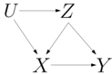3 If an exogenous variable feeds into more than one causal mechanism, the model is said to be semi-Markovian . In this case, interventional probabilities are identifiable only when certain conditions are met. The causal graph on the right corresponds to a semi-Markovian model since U feeds into the causal mechanisms for both X and Z . The causal effect Pr ( y x ) is identifiable since Pr ( y x ) = ∑ z Pr ( y | x, z ) Pr ( z ) . <details> <summary>Image 5 Details</summary>  ### Visual Description ## Diagram: Causal Diagram ### Overview The image presents a causal diagram illustrating relationships between variables U, Z, X, and Y. The diagram uses arrows to indicate the direction of causal influence between these variables. ### Components/Axes * **Nodes:** The diagram contains four nodes labeled U, Z, X, and Y. * **Edges:** The diagram contains edges (arrows) indicating causal relationships. The arrows point from the cause to the effect. * **Arrows:** * U -> Z * U -> X * Z -> X * Z -> Y * X -> Y ### Detailed Analysis or Content Details The diagram shows the following causal relationships: * Variable U influences both Z and X. * Variable Z influences both X and Y. * Variable X influences Y. ### Key Observations * U is a common cause of Z and X. * Z is a common cause of X and Y. * X is a direct cause of Y. ### Interpretation The diagram represents a causal model where U affects Z and X, Z affects X and Y, and X affects Y. This model suggests that changes in U can indirectly affect Y through Z and X, and changes in Z can indirectly affect Y through X. The diagram is useful for understanding potential confounding variables and causal pathways in a system. </details> However, the causal effect Pr ( x z ) is not identifiable as it cannot be uniquely determined based on the causal graph and the distribution Pr ( X,Y,Z ) . The do-calculus provides a complete and efficient characterization of identifiable, interventional probabilities based on observational data [25, 35, 34]; see also [20]. 4 It is based on a set of rules that can be used to transform an interventional probability into a formula that includes only associational probabilities (we will call this an identifiability formula ). If the rules fail to make such a derivation, then the interventional probability is not identifiable. Other methods such as back-door [24] and front-door [29] provide simpler but incomplete tests and lead to simple identifiability formulas. For example, the back-door and front-door formulas have the forms Pr ( y x ) = ∑ z Pr ( y | x , z ) Pr ( z ) and Pr ( y x ) = ∑ z Pr ( z | x ) ∑ x ′ Pr ( y | x ′ , z ) Pr ( x ′ ) , where Z is called a back-door or front-door, respectively. A more refined identifiability test that utilizes contextspecific independence relations was proposed recently [36], thus expanding the reach of cross-layer causal inference. These relations correspond to equating certain parameters and can be integrated into circuits [5] to reduce the number of estimands. In summary, we can compute causal effects on semi-Markovian models using circuits parameterized by maximum-likelihood estimates, but only for identifiable queries as licensed by the do-calculus or a more refined identifiability procedure. Identifiability Formulas vs Circuits Most identifiability procedures yield formulas (also called the effect estimand ) which play three roles: they provide a proof of identifiability; they point to endogenous variables whose measurement guarantees identifiability; and they allow one to evaluate the causal effect by estimating quantities that populate such formulas. Back-door and front-door formulas have simple forms (albeit exponential sums) but the do-calculus and the procedure in [36] may generate identifiability formulas that are much more complex. Some procedures do not even aim to produce identifiability formulas; e.g., [19]. To evaluate causal effects using circuits, one only needs an identifiability test not a formula. That is, one estimates circuit parameters only once and then uses the parametrized circuit to answer any identifiable query in time linear in the circuit size-regardless of how complex the identifiability formula may be and without needing to have access to one. 5 Additional knowledge such as context-specific independence and known mechanisms can be directly integrated into the circuit [5], which can only improve the quality of estimates under finite data. At its core, this use of circuits amounts to computing causal effects based on the classical method of mutilating causal graphs, armed by an observation and an advance. The observation is that using maximum-likelihood parameters is sound if the causal effect is identifiable. The advance is that we can now perform this computation much more efficiently due to exploiting unknown mechanisms. The Circuit Compilation Process Wewill next discuss the circuit compilation algorithm introduced recently in [15]. We will focus on the key insights behind the algorithm and slightly adjust it to suit our current objectives (the original algorithm targetted specific queries as is typically demanded in a supervised learning setting). In a nutshell, the algorithm is based on the classical algorithm of variable elimination (VE) with two exceptions. First, we will use VE symbolically by working with symbolic parameters instead of numeric ones. Second, we will empower VE by two new theorems based on unknown causal mechanisms which can reduce its complexity exponentially. We will review VE in Section 4 and then present the new theorems and compilation algorithm in Sections 5 and 6. 3 See [34, Corollary 4] for a weaker, necessary condition that guarantees identifiability of all causal effects. 4 See also [22] for a treatment of identifiability based on both observational and interventional data and [3] for a survey that considers other tasks such as the evaluation of soft interventions. 5 Using circuits in this manner requires fixing the cardinality of variables including exogenous ones. ## 4 The Variable Elimination Algorithm ( VE ) VE operates on causal graphs which are parameterized by factors. A factor over variables X is a function f ( X ) that maps each instantiation x into a number f ( x ) . For each node X and its parents P in the causal graph, we need a factor f X ( X, P ) where f X ( x, p ) = Pr ( x | p ) . For example, factor f ( U ) on the right specifies the distribution Pr ( U ) for exogenous variable U and factor g ( XY ) specifies the mechanism for endogenous variable Y : x 0 ↦→ y 1 , x 1 ↦→ y 0 . VE is based | U u | X Y x 0 y 0 | |-------|---------------| two factor operations: multiplication and sum-out. The product of factors f ( X ) and g ( Y ) is another factor h ( Z ) , where Z = X ∪ Y and h ( z ) = f ( x ) g ( y ) for the unique instantiations x and y that are compatible with instantiation z . Summing-out variables Y ⊆ X from factor f ( X ) yields another factor g ( Z ) , where Z = X \ Y and g ( z ) = ∑ y f ( yz ) . We use ∑ Y f to denote the resulting factor g . The joint distribution of a parametrized causal graph is simply the product of its factors. The causal graph in Figure 1(b) has factors f A ( A ) , f B ( AB ) , f C ( AC ) , f D ( BCD ) and f E ( CE ) . Its joint distribution is Pr ( ABCDE ) = f A f B f C f D f E . To record an observation X = x , we use an auxiliary evidence factor λ X ( X ) with λ X ( x ) = 1 and λ X ( x ′ ) = 0 for x ′ = x . A posterior distribution is obtained by normalizing the product of all factors in the causal graph including evidence factors. Suppose we have evidence e on variables A and E in Figure 1(b). The posterior Pr ( D | e ) is obtained by evaluating then normalizing the expression ∑ ABCE λ A λ E f A f B f C f D f E . VE tries to evaluate such expressions efficiently [38, 17] based on two theorems; see, e.g., [14, Chapter 6]. The first theorem allows us to sum out variables in any order. The second theorem allows us to pull out factors from sums, which can lead to exponential savings in time and space. <!-- formula-not-decoded --> Theorem 2. If variables X appear in factor f but not in factor g , then ∑ X f · g = g ∑ X f . Consider the expression ∑ ABDE f ( ACE ) f ( BCD ) . A direct evaluation multiplies the two factors to yield f ( ABCDE ) then sums out variables ABDE . Using Theorem 1, we can arrange the expression into ∑ AE ∑ BD f ( ACE ) f ( BCD ) . Using Theorem 2, we can arrange it further into ∑ AE f ( ACE ) ∑ BD f ( BCD ) which is more efficient to evaluate. If we eliminate all variables using order π , and if the largest factor constructed in the process has w +1 variables, then w is called the width of order π . The smallest width attained by any elimination order corresponds to the treewidth of the causal graph. The best time complexity that can be attained by VE is O ( n exp( w )) , where n is the number of variables and w is the causal graph treewidth. This holds for any other non-parametric method known today (i.e., inference methods that do not exploit the graph parameters). ## 5 Variable Elimination with Causal Mechanisms We next present two recent results that allow us to simplify expressions beyond what is permitted by Theorems 1 and 2, leading to a tighter complexity based on what we shall call the causal treewidth. We will use F , G , H to denote sets of factors, where each set is interpreted as a product of its factors. Definition 5. A factor f ( X, P ) is said to be a 'mechanism' for variable X iff all numbers in the factor are in { 0 , 1 } and ∑ x f ( x, p ) = 1 for every instantiation p . Theorem 3 ([15]) . Let f be a mechanism for variable X . If f ∈ G and f ∈ H , then G·H = G ∑ X H . According to this result, if a mechanism for X appears in both parts of a product, then variable X can be summed out from one part without changing the value of the product. This has a key corollary. Corollary 1. Let f be a mechanism for X . If f ∈ G and f ∈ H , then ∑ X G·H = ( ∑ X G ) ( ∑ X H ) . That is, if a mechanism for X appears in both parts of a product, we can sum out variable X from the product by independently summing it out from each part. This is a remarkable addition to the algorithm of variable elimination which has been under study for a few decades now. Corollary 1 may appear unusable as it is predicated on multiple occurrences of a mechanism whereas the factors of a causal graph contain a single mechanism for each endogenous variable. This is where the second result comes in: replicating mechanisms in a product does not change the product value. Theorem 4 ([15]) . For mechanism f , if f ∈ G , then f · G = G . For an example that uses these theorems, consider the expression α = ∑ X f ( XY ) g ( XZ ) h ( XW ) . VE has to multiply all three factors before summing out variable X , leading to a factor over four variables XYZW . However, if factor f is a mechanism for variable X , then we can replicate it by Theorem 4: α = f ( XY ) g ( XZ ) f ( XY ) h ( XW ) . Corollary 1 then gives α = ∑ X f ( XY ) g ( XZ ) ∑ X f ( XY ) h ( XW ) . Hence, we can now evaluate expression α without having to construct any factor over more than three variables. This technique can more generally lead to exponential savings since the size of a factor is exponential in the number of its variables. We will refer to the extension of VE with Theorems 3 and 4 as VEC ( V ariable E limination for C ausality). We emphasize that these new theorems do not require the values of parameters (i.e., specific mechanisms). They only need to know if a variables is functionally determined by its parents. ## 6 Compiling Causal Graphs Into Circuits We next show how VE/VEC can be used symbolically to compile non-parametric causal graphs into arithmetic circuits with symbolic parameters. We will first show this concretely on a small example using VE, then discuss a general compilation algorithm based on VE and finally based on VEC. Consider the causal graph U → V with binary variables. The parameters of this graph are given by the factors f ( U ) and g ( UV ) shown on the right. We also added an evidence factor for endogenous variable V as it will be measured. These factors have symbolic parameters instead of numeric ones. | U | f ( U ) | U u | V g ( UV v θ v | u | V | h ( V ) | |-----|-----------|-------|---------------------------|-----|-----------| | u | θ u | u | ¯ v θ ¯ v | u | v | λ v | | ¯ u | θ ¯ u | ¯ u | v θ v | ¯ u | ¯ v | λ ¯ v | | | | ¯ u | ¯ v θ ¯ v | ¯ u | | | We will further overload the + and ∗ operators so they now construct circuit nodes instead of performing numeric operations. That is, each entry in the above factors can be viewed as a leaf circuit node. When multiplying, say, node θ u with node θ v | u , we construct a circuit node with ∗ as its label and nodes θ u , θ v | u as its children. And similarly for addition. We can now get a circuit for the causal graph by multiplying all its factors, including evidence factors, and then summing out all variables, AC = ∑ UV f ( U ) g ( UV ) h ( V ) . The resulting factor AC will have a single entry which contains the root of compiled circuit λ v ∗ θ u ∗ θ v | u + λ ¯ v ∗ θ u ∗ θ ¯ v | u + λ v ∗ θ ¯ u ∗ θ v | ¯ u + λ ¯ v ∗ θ ¯ u ∗ θ ¯ v | ¯ u . The equivalent expression AC = ∑ V h ( V ) ∑ U f ( U ) g ( UV ) gives the circuit λ v ∗ ( θ u ∗ θ v | u + θ ¯ u ∗ θ v | ¯ u ) + λ ¯ v ∗ ( θ u ∗ θ ¯ v | u + θ ¯ u ∗ θ ¯ v | ¯ u ) . Hence, the size and shape of a compiled circuit depend on how we schedule factor operations (multiplication and sum-out). The symbolic use of VE to compile circuits was initially proposed in [6]. This method was recently refined in [15] by (1) scheduling factor operations based on a specific class of binary jointrees [33] and (2) allowing one to compile circuits using VEC by thinning the jointree. We will explain this advance after a brief review of (binary) jointrees. 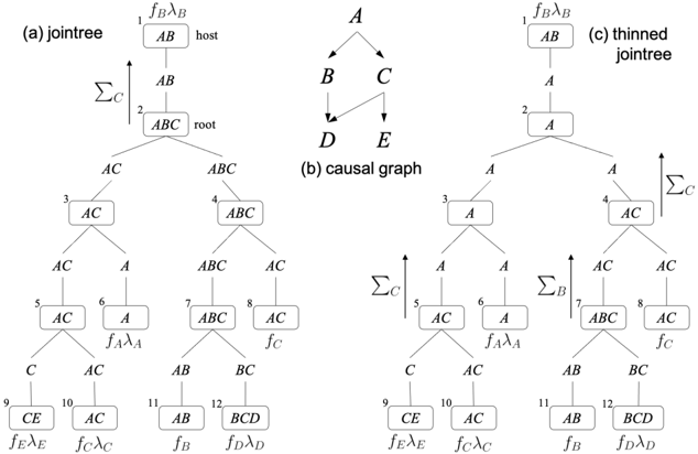Jointrees A binary jointree is a tree in which each node is either a leaf (has a single neighbor) or internal (has three neighbors). We will require the leaf nodes to be in one-to-one correspondence with the factors of a causal graph, including replicated factors but excluding evidence factors. As we show next, the topology of a binary jointree determines all its properties, including the set of variables attached to each node, called a cluster, and the set of variables attached to each edge, called a separator. Figure 1(a) depicts a binary jointree for the causal graph in Figure 1(b). Following the convention in [15], this jointree is layed out so that each internal node has two neighbors below it (children) and the third neighbor above it (parent). The leaf nodes of this jointree are numbered 1 , 6 , 8 , 9 , 10 , 11 , 12 and correspond to the causal graph factors, f B , f A , f C , f E , f C , f B , f D (we replicated the factors for B and C ). The separator for edge ( i, j ) between node i and its parent j is denoted sep ( i ) and contains variables that are shared between factors on both sides of the edge ( i, j ) . For example, sep (3) = { A,C } as these are the variables shared between factors at leaves { 6 , 9 , 10 } and factors at leaves { 1 , 8 , 11 , 12 } . The cluster of node i is denoted cls ( i ) . The cluster of a leaf node is the variables of its associated factor. The cluster of an internal node is the union of separators connected to its children. For example, for leaf node 9 with factor f E , cls (9) = vars ( f E ) = { C, E } . Moreover, for internal node 7 with children 11 and 12 , cls (7) = sep (11) ∪ sep (12) = { A,B,C } . Scheduling Given a binary jointree, VE (and later VEC) schedules its operations as follows. Visiting nodes bottom-up in the jointree, each node i computes a factor f ( i ) and sends it to its parent. A leaf node i computes f ( i ) by projecting its associated factor on sep ( i ) . For example, f (9) = ∑ E f E λ E . An internal node i computes f ( i ) by multiplying the factors it receives from its children and then projecting the product on sep ( i ) . For example, f (2) = ∑ C f (3) f (4) . This process terminates at the Figure 1: A causal graph (middle) with a jointree (left) and a thinned jointree (right). The mechanisms for variables B and C , f B and f C , are replicated twice in the jointrees. <details> <summary>Image 6 Details</summary>  ### Visual Description ## Diagram: Jointree, Causal Graph, and Thinned Jointree ### Overview The image presents three diagrams: a jointree, a causal graph, and a thinned jointree. These diagrams illustrate relationships between variables, potentially in the context of probabilistic graphical models or Bayesian networks. The jointree diagrams show a hierarchical structure with nodes labeled with variable sets, while the causal graph depicts direct dependencies between variables. The thinned jointree is a simplified version of the jointree. ### Components/Axes **(a) Jointree:** * **Nodes:** Rectangular boxes containing sets of variables (e.g., AB, ABC, AC, A, BC, BCD, CE). Each node is numbered from 1 to 12. * **Edges:** Lines connecting the nodes, indicating relationships or message passing. * **Labels:** * Node 1: "fBλB" (top-left of the node), "host" (top-right of the node) * Node 2: "root" (right of the node) * Node 6: "fAλA" (below the node) * Node 8: "fC" (below the node) * Node 9: "fEλE" (below the node) * Node 10: "fCλC" (below the node) * Node 11: "fB" (below the node) * Node 12: "fDλD" (below the node) * **Arrow:** An upward-pointing arrow labeled "ΣC" indicates a summation or marginalization operation. **(b) Causal Graph:** * **Nodes:** Labeled A, B, C, D, and E. * **Edges:** Directed arrows indicating causal relationships. A causes B and C. B causes D. C causes E. **(c) Thinned Jointree:** * **Nodes:** Rectangular boxes containing sets of variables (A, AC, AB, BCD, CE). Each node is numbered from 1 to 12. * **Edges:** Lines connecting the nodes. * **Labels:** * Node 1: "fBλB" (top-left of the node) * Node 6: "fAλA" (below the node) * Node 8: "fC" (below the node) * Node 9: "fEλE" (below the node) * Node 10: "fCλC" (below the node) * Node 11: "fB" (below the node) * Node 12: "fDλD" (below the node) * **Arrows:** Upward-pointing arrows labeled "ΣC" and "ΣB" indicate summation or marginalization operations. ### Detailed Analysis or Content Details **Jointree (a):** * Node 1 (AB) is the host. * Node 2 (ABC) is the root. * The tree branches from the root (ABC) to nodes 3 (AC) and 4 (ABC). * Node 3 (AC) branches to nodes 5 (AC) and 6 (A). * Node 4 (ABC) branches to nodes 7 (ABC) and 8 (AC). * Node 5 (AC) branches to nodes 9 (CE) and 10 (AC). * Node 7 (ABC) branches to nodes 11 (AB) and 12 (BCD). **Causal Graph (b):** * A is the parent node of B and C. * B is the parent node of D. * C is the parent node of E. **Thinned Jointree (c):** * Node 1 (AB) is at the top. * Node 2 (A) is below Node 1. * The tree branches from Node 2 (A) to nodes 3 (A) and 4 (AC). * Node 3 (A) branches to nodes 5 (AC) and 6 (A). * Node 4 (AC) branches to nodes 7 (ABC) and 8 (AC). * Node 5 (AC) branches to nodes 9 (CE) and 10 (AC). * Node 7 (ABC) branches to nodes 11 (AB) and 12 (BCD). ### Key Observations * The jointree and thinned jointree represent factorized probability distributions. * The causal graph shows the dependencies between variables. * The thinned jointree is a simplified version of the jointree, potentially optimized for inference. * The "Σ" symbols indicate marginalization operations, which are used to eliminate variables from the distribution. ### Interpretation The diagrams illustrate the process of converting a causal model (represented by the causal graph) into a form suitable for efficient inference (represented by the jointree and thinned jointree). The causal graph explicitly shows the dependencies between variables, while the jointree represents the joint probability distribution in a factorized form. The thinned jointree is a further simplification, potentially achieved by eliminating redundant variables or factors. The marginalization operations (ΣC, ΣB) are used to compute marginal probabilities by summing over the possible values of the eliminated variables. The labels "fBλB", "fAλA", etc., likely represent factors in the joint probability distribution. The "host" and "root" labels in the jointree indicate specific roles of nodes in the message-passing process. </details> top leaf node r which multiplies the factor it receives from its single child c with its own factor and then projects the product on the empty set. In Figure 1(a), the final computation is ∑ AB f B λ B f (2) . Denoting the factor at leaf node i by F i , this process yields the factor AC = ∑ cls ( r ) F r f ( c ) , where <!-- formula-not-decoded --> The final factor AC has a single entry which contains the root of the compiled circuit as shown earlier. Moreover, the size of this circuit is determined by the jointree clusters and separators. Each cluster/separator contributes a number of multiplication/addition nodes that is exponential in the cluster/separator size. In a jointree, the largest cluster dominates the largest separator and the size of the largest cluster minus 1 is called the jointree width. Furthermore, the smallest width attained by any jointree corresponds to the treewidth of the causal graph; see, [14, Chapter 9]. Hence, the complexity of this compilation method is exponential in the treewidth of the causal graph. Thinning This complexity was recently significantly improved by exploiting (unknown) causal mechanisms [15]. The basic idea is to thin the jointree by shrinking its separators (and hence clusters) while maintaining the correctness of compiled circuit. The thinning process is based on Theorems 3 and 4 and can lead to an exponential reduction in the circuit size. To see the key insight behind this thinning process, consider node 2 in the jointree of Figure 1(a). The separators sep (3) and sep (4) of its children both contain variable C . Hence, the factors f (3) and f (4) sent by these children to node 2 both contain variable C . Since C does not appear in sep (2) it gets summed out at node 2 so it does not appear in the factor f (2) that this node sends to its parent. However, since we have two replicas of the mechanism for variable C at leaf nodes 8 and 10 (as licensed by Theorem 4), we can sum out C earlier, at nodes 4 and 5 (as licensed by Theorem 3). This means that C can be removed from sep (4) , sep (5) and also sep (3) . We can similarly sum out variable B at node 7 , which removes it from sep (7) , sep (4) and sep (2) . The shrinking of separators causes clusters to shrink as well, leading to the thinned jointree in Figure 1(c) and a corresponding smaller circuit compilation. Causal Treewidth The attained reduction in complexity depends on (1) the number of replicas for each mechanism; (2) the used binary jointree; and (3) how the jointree is thinned. Corresponding heuristics were proposed in [15] and the resulting algorithm was shown to yield exponential reductions in the size of compiled circuits on a number of benchmarks (elimination orders and jointrees are also constructed using heuristics since finding optimal ones is NP-hard). This motivates a new measure of complexity which we call the causal treewidth. We define this as the smallest width attained by any thinned jointree for a given causal graph. We next complement the empirical findings in [15] by showing that causal treewidth dominates treewidth and can be bounded when the treewidth is not. Figure 2: A causal graph and its thinned jointree. Mechanisms f X i and f Y j are replicated n times. <details> <summary>Image 7 Details</summary>  ### Visual Description ## Diagram: Causal Graph and Jointree Representations ### Overview The image presents three related diagrams: a causal graph, a thinned jointree, and a jointree fragment. These diagrams likely represent a probabilistic model or inference process. The causal graph shows dependencies between variables, while the jointrees represent factorizations of the joint probability distribution. ### Components/Axes * **(a) causal graph for n=3:** This is a directed acyclic graph (DAG) representing causal relationships between variables. * Nodes: Labeled as U_X, U_Y, X₁, Y₁, X₂, Y₂, X₃, Y₃, Z₁₁, Z₁₂, Z₁₃, Z₂₁, Z₂₂, Z₂₃, Z₃₁, Z₃₂, Z₃₃. * Edges: Represented by lines connecting the nodes, indicating dependencies. U_X and U_Y are at the top, followed by X_i and Y_i, and then Z_ij at the bottom. * **(b) thinned jointree:** This is a tree structure representing a factorization of the joint probability distribution. * Nodes: Labeled with variable sets (e.g., f_UX U_X, U_X, U_XU_Y, U_Y) or T(i,j) where i and j are indices. * Edges: Connect the nodes, representing conditional dependencies. * Nodes are arranged hierarchically, starting from f_UX U_X at the top and branching down to T(1,1), T(1,2), and eventually T(n,n) at the bottom. * **(c) jointree fragment:** This is a detailed view of a portion of a jointree. * Nodes: Labeled with variable sets (e.g., U_XU_Y, Y_jU_X, Y_jU_Y, X_iY_jU_X, Y_jU_Y, X_iY_j, X_iU_X, X_iY_jZ_ij, X_iU_X) or factors (e.g., f_Yj, f_Zij, f_Xi). * Edges: Connect the nodes, representing conditional dependencies. ### Detailed Analysis or Content Details * **Causal Graph:** * U_X and U_Y are parent nodes, influencing X_i and Y_i respectively. * X_i and Y_j influence Z_ij. * The graph is for n=3, indicating three X and Y variables. * **Thinned Jointree:** * The tree starts with f_UX U_X at the root. * The tree branches down, with nodes labeled U_XU_Y. * Nodes labeled T(1,1), T(1,2), and T(n,n) are present, suggesting a pattern. * A dashed line indicates a continuation of the tree structure. * **Jointree Fragment:** * The fragment shows a detailed factorization of a portion of the jointree. * Nodes are labeled with variable sets and factors. * The structure represents conditional dependencies between variables. ### Key Observations * The causal graph provides a high-level view of the dependencies between variables. * The thinned jointree represents a factorization of the joint probability distribution. * The jointree fragment provides a detailed view of a portion of the jointree. * The diagrams are related, with the jointrees representing factorizations derived from the causal graph. ### Interpretation The image illustrates the relationship between a causal graph and its corresponding jointree representation. The causal graph defines the dependencies between variables, while the jointree represents a factorization of the joint probability distribution that respects these dependencies. The thinned jointree provides a simplified view of the jointree, while the jointree fragment shows a detailed portion of the factorization. These diagrams are used in probabilistic inference to efficiently compute probabilities and make predictions. The T(i,j) nodes likely represent intermediate computations or marginalizations over subsets of variables. The dashed line in the thinned jointree indicates that the tree structure continues, suggesting that the full jointree may be more complex than what is shown. 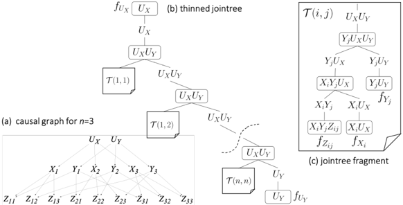</details> Theorem 5. The causal treewidth is no greater than treewidth. Moreover, there is a family of causal graphs with n 2 +2 n +1 variables, treewidth n +1 and causal treewidth 2 where n is an integer ≥ 1 . Proof Sketch. Consider a causal graph G with treewidth w . Without replicating mechanisms, we can always get a (thinned) jointree with width w . Hence, the causal treewidth of G is ≤ w . To show the second part of the theorem, consider the family of causal graphs G n with exogenous variables U X , U Y and endogenous variables X i , Y j , Z ij for i, j = 1 , . . . , n ( 2 + 2 n + n 2 variables), and edges U X → X i , U Y → Y j , X i → Z ij , Y j → Z ij . Figure 2(a) depicts G 3 . We next show that G n has treewidth n +1 based on standard techniques for treewidth; see, e.g., [14, Chapter 9]. The moral graph of G n is obtained by dropping edge directions and connecting every pair of nodes X i and Y j by an undirected edge. Each Z ij has only two (connected) neighbors in the moral graph ( X i and Y j ) so it is a simplicial node. Hence, there must exist an optimal elimination order that starts with nodes Z ij [14, Section 9.3.2]. After eliminating all Z ij , nodes U X and U Y will each have n neighbors, and nodes X i and Y j will each have n +1 neighbors. A simple argument shows that eliminating these variables in any order from the moral graph will create a clique over n +1 variables so the treewidth is ≥ n +1 . One can easily verify that the elimination order Z 11 , . . . , Z nn , U X , Y 1 , . . . , Y n , U Y , X 1 , . . . , X n has width n +1 so the treewidth of G n is n +1 . Figure 2(b) depicts a thinned jointree for G n with width 2 , which results from cascading n 2 instances of the jointree fragment T ( i, j ) in Figure 2(c). This fragment contains the mechanism for Z ij and replicas of the mechanisms for X i and Y j . This thinned jointree is optimal since the mechanism for Z ij contains 3 variables so any thinned jointree must have a cluster of size ≥ 3 . Hence, the causal treewidth of G n is 2 . Theorem 5 effectively says that circuits compiled by VEC are no larger than those compiled by VE and can be exponentially smaller. We finally note that a variation G ′ n on G n was shown in Section 3 with additional edges between variables Z ij . The treewidth of G ′ n must be ≥ n +1 yet has a thinned jointree of width 4 (constructed by the algorithm in [15]) so its causal treewidth is ≤ 4 . Recall that for this family of causal graphs G ′ n , the causal effect of X 1 on Z nn has the only back-door X 2 , . . . , X n so it has a back-door formula with a sum that is exponential in n and a circuit of size O ( n 2 ) . ## 7 Conclusion We discussed recent techniques that can exploit causal mechanisms computationally without having to know their identities, which is the classical setup in causal inference. We also showed how one can use these techniques to compile non-parametric causal graphs into circuits that can be used to estimate parameters from data and to perform cross-layer causal inference in time linear in the circuit size. Our aim was to provide an intuitive exposure to these techniques to a causality audience who may not be as familiar with them, with the hope that this may lead to a synthesis on how tractable arithmetic circuits can aid causal inference in reaching higher levels of scalability and versatility. Acknowledgements I wish to thank Elias Bareinboim, Yizuo Chen, Scott Mueller, Judea Pearl and Jin Tian for useful discussions and feedback. This work has been partially supported by NSF grant #ISS-1910317 and ONR grant #N00014-18-1-2561. ## References - [1] Durgesh Agrawal, Yash Pote, and Kuldeep S. Meel. Partition function estimation: A quantitative study. In IJCAI , pages 4276-4285. ijcai.org, 2021. - [2] E. Bareinboim, Juan David Correa, D. Ibeling, and Thomas F. Icard. On Pearl's hierarchy and the foundations of causal inference. 2021. Technical Report, R-60, Colombia University. - [3] Elias Bareinboim and Judea Pearl. Causal inference and the data-fusion problem. Proc. Natl. Acad. Sci. USA , 113(27):7345-7352, 2016. - [4] Craig Boutilier, Nir Friedman, Moisés Goldszmidt, and Daphne Koller. Context-specific independence in Bayesian networks. CoRR , abs/1302.3562, 2013. - [5] Mark Chavira and Adnan Darwiche. Compiling Bayesian networks with local structure. In Leslie Pack Kaelbling and Alessandro Saffiotti, editors, IJCAI-05, Proceedings of the Nineteenth International Joint Conference on Artificial Intelligence, Edinburgh, Scotland, UK, July 30 August 5, 2005 , pages 1306-1312. Professional Book Center, 2005. - [6] Mark Chavira and Adnan Darwiche. Compiling Bayesian networks using variable elimination. In Proceedings of the 20th International Joint Conference on Artificial Intelligence (IJCAI) , pages 2443-2449, 2007. - [7] Mark Chavira and Adnan Darwiche. On probabilistic inference by weighted model counting. Artif. Intell. , 172(6-7):772-799, 2008. - [8] Mark Chavira, Adnan Darwiche, and Manfred Jaeger. Compiling relational Bayesian networks for exact inference. Int. J. Approx. Reason. , 42(1-2):4-20, 2006. - [9] Yizuo Chen, Arthur Choi, and Adnan Darwiche. Supervised learning with background knowledge. In PGM , 2020. - [10] Arthur Choi and Adnan Darwiche. On relaxing determinism in arithmetic circuits. In Proceedings of the Thirty-Fourth International Conference on Machine Learning (ICML) , pages 825-833, 2017. - [11] Arthur Choi, Doga Kisa, and Adnan Darwiche. Compiling probabilistic graphical models using sentential decision diagrams. In ECSQARU , volume 7958 of Lecture Notes in Computer Science , pages 121-132. Springer, 2013. - [12] Adnan Darwiche. A logical approach to factoring belief networks. In Dieter Fensel, Fausto Giunchiglia, Deborah L. McGuinness, and Mary-Anne Williams, editors, Proceedings of the Eights International Conference on Principles and Knowledge Representation and Reasoning (KR-02), Toulouse, France, April 22-25, 2002 , pages 409-420. Morgan Kaufmann, 2002. - [13] Adnan Darwiche. A differential approach to inference in Bayesian networks. J. ACM , 50(3):280305, 2003. - [14] Adnan Darwiche. Modeling and Reasoning with Bayesian Networks . Cambridge University Press, 2009. - [15] Adnan Darwiche. An advance on variable elimination with applications to tensor-based computation. In ECAI , volume 325 of Frontiers in Artificial Intelligence and Applications , pages 2559-2568. IOS Press, 2020. - [16] Adnan Darwiche. Tractable Boolean and arithmetic circuits. In Pascal Hitzler and Md Kamruzzaman Sarker, editors, Neuro-symbolic Artificial Intelligence: The State of the Art . Frontiers in Artificial Intelligence and Applications. IOS Press, 2022. In print. - [17] Rina Dechter. Bucket elimination: A unifying framework for probabilistic inference. In Proceedings of the Twelfth Annual Conference on Uncertainty in Artificial Intelligence (UAI) , pages 211-219, 1996. - [18] Paulius Dilkas and Vaishak Belle. Weighted model counting with conditional weights for Bayesian networks. In UAI , 2021. - [19] Joseph Y. Halpern. Axiomatizing causal reasoning. J. Artif. Intell. Res. , 12:317-337, 2000. - [20] Yimin Huang and Marco Valtorta. Identifiability in causal bayesian networks: A sound and complete algorithm. In AAAI , pages 1149-1154. AAAI Press, 2006. - [21] Madelyn Glymour Judea Pearl and Nicholas P. Jewell. Causal Inference in Statistics: A Primer . Wiley, 2016. - [22] Sanghack Lee, Juan D. Correa, and Elias Bareinboim. General identifiability with arbitrary surrogate experiments. In UAI , volume 115 of Proceedings of Machine Learning Research , pages 389-398. AUAI Press, 2019. - [23] Daniel Lowd and Pedro M. Domingos. Learning arithmetic circuits. In Proceedings of the 24th Conference in Uncertainty in Artificial Intelligence (UAI) , pages 383-392, 2008. - [24] Judea Pearl. [bayesian analysis in expert systems]: Comment: Graphical models, causality and intervention. Statistical Science , 8(3):266-269, 1993. - [25] Judea Pearl. Causal diagrams for empirical research. Biometrika , 82(4):669-688, 1995. - [26] Judea Pearl. Causality . Cambridge University Press, 2000. - [27] Judea Pearl. The seven tools of causal inference, with reflections on machine learning. Commun. ACM , 62(3):54-60, 2019. - [28] Judea Pearl and Dana Mackenzie. The Book of Why: The New Science of Cause and Effect . Basic Books, 2018. - [29] Judea Pearl and James M. Robins. Probabilistic evaluation of sequential plans from causal models with hidden variables. In Philippe Besnard and Steve Hanks, editors, UAI '95: Proceedings of the Eleventh Annual Conference on Uncertainty in Artificial Intelligence, Montreal, Quebec, Canada, August 18-20, 1995 , pages 444-453. Morgan Kaufmann, 1995. - [30] Hoifung Poon and Pedro M. Domingos. Sum-product networks: A new deep architecture. In UAI , pages 337-346. AUAI Press, 2011. - [31] Biao Qin. Differential semantics of intervention in Bayesian networks. In IJCAI , pages 710-716. AAAI Press, 2015. - [32] Yujia Shen, Arthur Choi, and Adnan Darwiche. Tractable operations for arithmetic circuits of probabilistic models. In NIPS , pages 3936-3944, 2016. - [33] Prakash P. Shenoy. Binary join trees. In UAI , pages 492-499. Morgan Kaufmann, 1996. - [34] Ilya Shpitser and Judea Pearl. Identification of joint interventional distributions in recursive semi-markovian causal models. In AAAI , pages 1219-1226. AAAI Press, 2006. - [35] Jin Tian and Judea Pearl. A general identification condition for causal effects. In AAAI/IAAI , pages 567-573. AAAI Press / The MIT Press, 2002. - [36] Santtu Tikka, Antti Hyttinen, and Juha Karvanen. Identifying causal effects via context-specific independence relations. In NeurIPS , pages 2800-2810, 2019. - [37] Benjie Wang, Clare Lyle, and Marta Kwiatkowska. Provable guarantees on the robustness of decision rules to causal interventions. In IJCAI , pages 4258-4265. ijcai.org, 2021. - [38] Nevin Lianwen Zhang and David Poole. Exploiting causal independence in bayesian network inference. Journal of Artificial Intelligence Research , 5:301-328, 1996.