2203.15556v1

<details> <summary>Image 1 Details</summary>  ### Visual Description Icon/Small Image (202x49) </details> ## Training Compute-Optimal Large Language Models Jordan Hoffmann ★ , Sebastian Borgeaud ★ , Arthur Mensch ★ , Elena Buchatskaya, Trevor Cai, Eliza Rutherford, Diego de Las Casas, Lisa Anne Hendricks, Johannes Welbl, Aidan Clark, Tom Hennigan, Eric Noland, Katie Millican, George van den Driessche, Bogdan Damoc, Aurelia Guy, Simon Osindero, Karen Simonyan, Erich Elsen, Jack W. Rae, Oriol Vinyals and Laurent Sifre ★ ★ Equal contributions We investigate the optimal model size and number of tokens for training a transformer language model under a given compute budget. We find that current large language models are significantly undertrained, a consequence of the recent focus on scaling language models whilst keeping the amount of training data constant. By training over 400 language models ranging from 70 million to over 16 billion parameters on 5 to 500 billion tokens, we find that for compute-optimal training, the model size and the number of training tokens should be scaled equally: for every doubling of model size the number of training tokens should also be doubled. We test this hypothesis by training a predicted computeoptimal model, Chinchilla , that uses the same compute budget as Gopher but with 70B parameters and 4 more more data. Chinchilla uniformly and significantly outperforms Gopher (280B), GPT-3 (175B), Jurassic-1 (178B), and Megatron-Turing NLG (530B) on a large range of downstream evaluation tasks. This also means that Chinchilla uses substantially less compute for fine-tuning and inference, greatly facilitating downstream usage. As a highlight, Chinchilla reaches a state-of-the-art average accuracy of 67.5% on the MMLU benchmark, greater than a 7% improvement over Gopher . ## 1. Introduction Recently a series of Large Language Models (LLMs) have been introduced (Brown et al., 2020; Lieber et al., 2021; Rae et al., 2021; Smith et al., 2022; Thoppilan et al., 2022), with the largest dense language models now having over 500 billion parameters. These large autoregressive transformers (Vaswani et al., 2017) have demonstrated impressive performance on many tasks using a variety of evaluation protocols such as zero-shot, few-shot, and fine-tuning. The compute and energy cost for training large language models is substantial (Rae et al., 2021; Thoppilan et al., 2022) and rises with increasing model size. In practice, the allocated training compute budget is often known in advance: how many accelerators are available and for how long we want to use them. Since it is typically only feasible to train these large models once, accurately estimating the best model hyperparameters for a given compute budget is critical (Tay et al., 2021). Kaplan et al. (2020) showed that there is a power law relationship between the number of parameters in an autoregressive language model (LM) and its performance. As a result, the field has been training larger and larger models, expecting performance improvements. One notable conclusion in Kaplan et al. (2020) is that large models should not be trained to their lowest possible loss to be compute optimal. Whilst we reach the same conclusion, we estimate that large models should be trained for many more training tokens than recommended by the authors. Specifically, given a 10 increase computational budget, they suggests that the size of the model should increase 5 5 while the number of training tokens should only increase 1.8 . Instead, we find that model size and the number of training tokens should be scaled in equal proportions. Following Kaplan et al. (2020) and the training setup of GPT-3 (Brown et al., 2020), many of the recently trained large models have been trained for approximately 300 billion tokens (Table 1), in line with the approach of predominantly increasing model size when increasing compute. 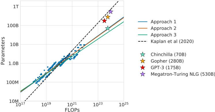Figure 1 j Overlaid predictions. We overlay the predictions from our three different approaches, along with projections from Kaplan et al. (2020). We find that all three methods predict that current large models should be substantially smaller and therefore trained much longer than is currently done. In Figure A3, we show the results with the predicted optimal tokens plotted against the optimal number of parameters for fixed FLOP budgets. Chinchilla outperforms Gopher and the other large models (see Section 4.2). <details> <summary>Image 2 Details</summary>  ### Visual Description ## Scatter Plot: Parameters vs. FLOPs for Different Language Models ### Overview The image is a scatter plot comparing the number of parameters of different language models against the number of floating-point operations (FLOPs) used to train them. The plot includes data points for several models, along with trend lines representing different approaches and a reference line from Kaplan et al. (2020). ### Components/Axes * **X-axis:** FLOPs (Floating Point Operations), with a logarithmic scale ranging from 10^17 to 10^25. * **Y-axis:** Parameters, with a logarithmic scale ranging from 10M (10^7) to 1T (10^12). * **Legend (Right side of the plot):** * Blue Line: Approach 1 * Orange Line: Approach 2 * Green Line: Approach 3 * Black Dashed Line: Kaplan et al (2020) * Light Blue Star: Chinchilla (70B) * Yellow Star: Gopher (280B) * Red Star: GPT-3 (175B) * Purple Star: Megatron-Turing NLG (530B) ### Detailed Analysis * **Approach 1 (Blue Line):** The blue line representing "Approach 1" shows a generally upward trend. * At 10^17 FLOPs, the parameters are approximately 20M. * At 10^21 FLOPs, the parameters are approximately 1B. * At 10^24 FLOPs, the parameters are approximately 100B. * **Approach 2 (Orange Line):** The orange line representing "Approach 2" also shows an upward trend, similar to Approach 1. * At 10^17 FLOPs, the parameters are approximately 20M. * At 10^21 FLOPs, the parameters are approximately 1B. * At 10^24 FLOPs, the parameters are approximately 100B. * **Approach 3 (Green Line):** The green line representing "Approach 3" shows an upward trend, similar to Approach 1 and Approach 2. * At 10^17 FLOPs, the parameters are approximately 20M. * At 10^21 FLOPs, the parameters are approximately 1B. * At 10^24 FLOPs, the parameters are approximately 100B. * **Kaplan et al (2020) (Black Dashed Line):** The black dashed line shows a steeper upward trend compared to the other approaches. * At 10^17 FLOPs, the parameters are approximately 10M. * At 10^21 FLOPs, the parameters are approximately 2B. * At 10^24 FLOPs, the parameters are approximately 200B. * **Chinchilla (Light Blue Star):** Located at approximately 10^23 FLOPs and 70B parameters. * **Gopher (Yellow Star):** Located at approximately 2 * 10^23 FLOPs and 280B parameters. * **GPT-3 (Red Star):** Located at approximately 2 * 10^23 FLOPs and 175B parameters. * **Megatron-Turing NLG (Purple Star):** Located at approximately 3 * 10^23 FLOPs and 530B parameters. * **Scatter Points (Blue Dots):** A cluster of blue dots is present, indicating a concentration of data points. These points generally follow the trend of Approach 1, Approach 2, and Approach 3. ### Key Observations * The three "Approach" lines are very close to each other, suggesting similar scaling relationships between FLOPs and parameters. * The Kaplan et al. (2020) line shows a steeper increase in parameters with respect to FLOPs compared to the other approaches. * The named models (Chinchilla, Gopher, GPT-3, Megatron-Turing NLG) are located towards the upper-right corner of the plot, indicating higher FLOPs and parameter counts. * The cluster of blue dots suggests a common trend among a larger set of models, with the named models representing outliers or models designed with different scaling strategies. ### Interpretation The plot illustrates the relationship between the computational cost (FLOPs) and the size (parameters) of language models. The different approaches likely represent different training methodologies or architectural choices. The Kaplan et al. (2020) line serves as a benchmark or theoretical scaling law. The positions of the named models relative to the trend lines indicate their efficiency or deviation from the general trends. For example, models above the trend lines are more parameter-efficient for a given FLOP count. The plot suggests that increasing both FLOPs and parameters generally leads to larger models, but the specific scaling relationship can vary depending on the approach used. </details> In this work, we revisit the question: Given a fixed FLOPs budget, 1 how should one trade-off model size and the number of training tokens? To answer this question, we model the final pre-training loss 2 𝐿 ' 𝑁 𝐷 ' as a function of the number of model parameters 𝑁 , and the number of training tokens, 𝐷 . Since the computational budget 𝐶 is a deterministic function FLOPs ' 𝑁 𝐷 ' of the number of seen training tokens and model parameters, we are interested in minimizing 𝐿 under the constraint FLOPs ' 𝑁 𝐷 ' = 𝐶 : <!-- formula-not-decoded --> The functions 𝑁𝑜𝑝𝑡 ' 𝐶 ' , and 𝐷𝑜𝑝𝑡 ' 𝐶 ' describe the optimal allocation of a computational budget 𝐶 . We empirically estimate these functions based on the losses of over 400 models, ranging from under 70M to over 16B parameters, and trained on 5B to over 400B tokens - with each model configuration trained for several different training horizons. Our approach leads to considerably different results than that of Kaplan et al. (2020). We highlight our results in Figure 1 and how our approaches differ in Section 2. Based on our estimated compute-optimal frontier, we predict that for the compute budget used to train Gopher , an optimal model should be 4 times smaller, while being training on 4 times more tokens. We verify this by training a more compute-optimal 70B model, called Chinchilla , on 1.4 trillion tokens. Not only does Chinchilla outperform its much larger counterpart, Gopher , but its reduced model size reduces inference cost considerably and greatly facilitates downstream uses on smaller hardware. The energy cost of a large language model is amortized through its usage for inference an fine-tuning. The benefits of a more optimally trained smaller model, therefore, extend beyond the immediate benefits of its improved performance. 1 For example, knowing the number of accelerators and a target training duration. 2 For simplicity , we perform our analysis on the smoothed training loss which is an unbiased estimate of the test loss, as we are in the infinite data regime (the number of training tokens is less than the number of tokens in the entire corpus). Table 1 j Current LLMs . We show five of the current largest dense transformer models, their size, and the number of training tokens. Other than LaMDA (Thoppilan et al., 2022), most models are trained for approximately 300 billion tokens. We introduce Chinchilla , a substantially smaller model, trained for much longer than 300B tokens. | Model | Size (# Parameters) | Training Tokens | |----------------------------------|-----------------------|-------------------| | LaMDA (Thoppilan et al., 2022) | 137 Billion | 168 Billion | | GPT-3 (Brown et al., 2020) | 175 Billion | 300 Billion | | Jurassic (Lieber et al., 2021) | 178 Billion | 300 Billion | | Gopher (Rae et al., 2021) | 280 Billion | 300 Billion | | MT-NLG 530B (Smith et al., 2022) | 530 Billion | 270 Billion | | Chinchilla | 70 Billion | 1.4 Trillion | ## 2. Related Work Large language models. A variety of large language models have been introduced in the last few years. These include both dense transformer models (Brown et al., 2020; Lieber et al., 2021; Rae et al., 2021; Smith et al., 2022; Thoppilan et al., 2022) and mixture-of-expert (MoE) models (Du et al., 2021; Fedus et al., 2021; Zoph et al., 2022). The largest dense transformers have passed 500 billion parameters (Smith et al., 2022). The drive to train larger and larger models is clear-so far increasing the size of language models has been responsible for improving the state-of-the-art in many language modelling tasks. Nonetheless, large language models face several challenges, including their overwhelming computational requirements (the cost of training and inference increase with model size) (Rae et al., 2021; Thoppilan et al., 2022) and the need for acquiring more high-quality training data. In fact, in this work we find that larger, high quality datasets will play a key role in any further scaling of language models. Modelling the scaling behavior. Understanding the scaling behaviour of language models and their transfer properties has been important in the development of recent large models (Hernandez et al., 2021; Kaplan et al., 2020). Kaplan et al. (2020) first showed a predictable relationship between model size and loss over many orders of magnitude. The authors investigate the question of choosing the optimal model size to train for a given compute budget. Similar to us, they address this question by training various models. Our work differs from Kaplan et al. (2020) in several important ways. First, the authors use a fixed number of training tokens and learning rate schedule for all models; this prevents them from modelling the impact of these hyperparameters on the loss. In contrast, we find that setting the learning rate schedule to approximately match the number of training tokens results in the best final loss regardless of model size-see Figure A1. For a fixed learning rate cosine schedule to 130B tokens, the intermediate loss estimates (for 𝐷 0 130B) are therefore overestimates of the loss of a model trained with a schedule length matching 𝐷 0 . Using these intermediate losses results in underestimating the effectiveness of training models on less data than 130B tokens, and eventually contributes to the conclusion that model size should increase faster than training data size as compute budget increases. In contrast, our analysis predicts that both quantities should scale at roughly the same rate. Secondly, we include models with up to 16B parameters, as we observe that there is slight curvature in the FLOP-loss frontier (see Appendix E)-in fact, the majority of the models used in our analysis have more than 500 million parameters, in contrast the majority of runs in Kaplan et al. (2020) are significantly smaller-many being less than 100M parameters. Recently, Clark et al. (2022) specifically looked in to the scaling properties of Mixture of Expert language models, showing that the scaling with number of experts diminishes as the model size increases-their approach models the loss as a function of two variables: the model size and the number of experts. However, the analysis is done with a fixed number of training tokens, as in Kaplan et al. (2020), potentially underestimating the improvements of branching. Estimating hyperparameters for large models. The model size and the number of training tokens are not the only two parameters to chose when selecting a language model and a procedure to train it. Other important factors include learning rate, learning rate schedule, batch size, optimiser, and width-to-depth ratio. In this work, we focus on model size and the number of training steps, and we rely on existing work and provided experimental heuristics to determine the other necessary hyperparameters. Yang et al. (2021) investigates how to choose a variety of these parameters for training an autoregressive transformer, including the learning rate and batch size. McCandlish et al. (2018) finds only a weak dependence between optimal batch size and model size. Shallue et al. (2018); Zhang et al. (2019) suggest that using larger batch-sizes than those we use is possible. Levine et al. (2020) investigates the optimal depth-to-width ratio for a variety of standard model sizes. We use slightly less deep models than proposed as this translates to better wall-clock performance on our hardware. Improved model architectures. Recently, various promising alternatives to traditional dense transformers have been proposed. For example, through the use of conditional computation large MoE models like the 1.7 trillion parameter Switch transformer (Fedus et al., 2021), the 1.2 Trillion parameter GLaM model (Du et al., 2021), and others (Artetxe et al., 2021; Zoph et al., 2022) are able to provide a large effective model size despite using relatively fewer training and inference FLOPs. However, for very large models the computational benefits of routed models seems to diminish (Clark et al., 2022). An orthogonal approach to improving language models is to augment transformers with explicit retrieval mechanisms, as done by Borgeaud et al. (2021); Guu et al. (2020); Lewis et al. (2020). This approach effectively increases the number of data tokens seen during training (by a factor of 10 in Borgeaud et al. (2021)). This suggests that the performance of language models may be more dependant on the size of the training data than previously thought. ## 3. Estimating the optimal parameter/training tokens allocation We present three different approaches to answer the question driving our research: Given a fixed FLOPs budget, how should one trade-off model size and the number of training tokens? In all three cases we start by training a range of models varying both model size and the number of training tokens and use the resulting training curves to fit an empirical estimator of how they should scale. We assume a power-law relationship between compute and model size as done in Clark et al. (2022); Kaplan et al. (2020), though future work may want to include potential curvature in this relationship for large model sizes. The resulting predictions are similar for all three methods and suggest that parameter count and number of training tokens should be increased equally with more compute 3 with proportions reported in Table 2. This is in clear contrast to previous work on this topic and warrants further investigation. 3 We compute FLOPs as described in Appendix F. 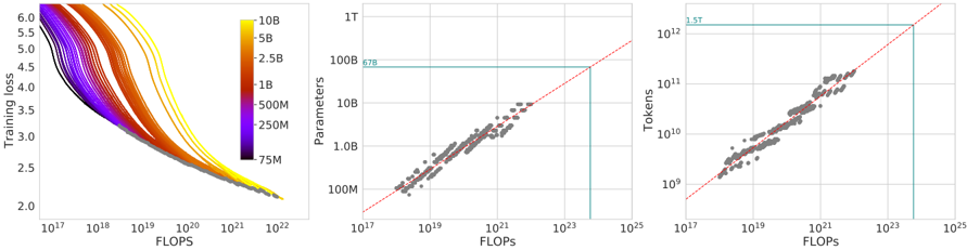Figure 2 j Training curve envelope. On the left we show all of our different runs. We launched a range of model sizes going from 70M to 10B, each for four different cosine cycle lengths. From these curves, we extracted the envelope of minimal loss per FLOP, and we used these points to estimate the optimal model size ( center ) for a given compute budget and the optimal number of training tokens ( right ). In green, we show projections of optimal model size and training token count based on the number of FLOPs used to train Gopher (5 76 10 23 ). <details> <summary>Image 3 Details</summary>  ### Visual Description ## Chart Type: Multiple Scatter Plots and Line Graph ### Overview The image consists of three plots. The first plot (left) shows training loss versus FLOPS, with different lines representing different model sizes (number of parameters). The second plot (center) shows the relationship between the number of parameters and FLOPS. The third plot (right) shows the relationship between the number of tokens and FLOPS. All plots use a logarithmic scale for both axes. ### Components/Axes **Plot 1 (Left): Training Loss vs. FLOPS** * **X-axis:** FLOPS (Floating Point Operations Per Second), logarithmic scale from approximately 10^17 to 10^22. * **Y-axis:** Training loss, linear scale from 2.0 to 6.0. * **Legend:** Located on the top-right of the plot. Represents the number of parameters in the model, with colors ranging from purple (75M) to yellow (10B). * Purple: 75M * Dark Blue: 250M * Blue: 500M * Green: 1B * Orange: 2.5B * Red: 5B * Yellow: 10B **Plot 2 (Center): Parameters vs. FLOPS** * **X-axis:** FLOPS, logarithmic scale from approximately 10^17 to 10^25. * **Y-axis:** Parameters, logarithmic scale from 100M to 1T (1 Trillion). * A red dashed line is present, indicating a linear relationship. * A horizontal teal line is present at approximately 678B parameters. **Plot 3 (Right): Tokens vs. FLOPS** * **X-axis:** FLOPS, logarithmic scale from approximately 10^17 to 10^25. * **Y-axis:** Tokens, logarithmic scale from 10^9 to 10^12 (1 Trillion). * A red dashed line is present, indicating a linear relationship. * A horizontal teal line is present at approximately 1.5T tokens. ### Detailed Analysis **Plot 1 (Left): Training Loss vs. FLOPS** * **Trend:** All lines show a decreasing trend, indicating that training loss decreases as FLOPS increase. * **Data Points:** * The line representing 75M parameters (purple) starts at a training loss of approximately 5.8 at 10^17 FLOPS and decreases to approximately 2.2 at 10^22 FLOPS. * The line representing 10B parameters (yellow) starts at a training loss of approximately 5.9 at 10^17 FLOPS and decreases to approximately 2.1 at 10^22 FLOPS. * The lines representing larger models (closer to yellow) tend to have slightly lower training loss for a given number of FLOPS compared to smaller models (closer to purple). **Plot 2 (Center): Parameters vs. FLOPS** * **Trend:** The data points show a positive correlation between the number of parameters and FLOPS. The points cluster around the red dashed line, indicating a roughly linear relationship on the log-log scale. * **Data Points:** * The data points range from approximately 100M parameters at 10^17 FLOPS to approximately 1T parameters at 10^23 FLOPS. * The teal line indicates a specific model size of 678B parameters. **Plot 3 (Right): Tokens vs. FLOPS** * **Trend:** The data points show a positive correlation between the number of tokens and FLOPS. The points cluster around the red dashed line, indicating a roughly linear relationship on the log-log scale. * **Data Points:** * The data points range from approximately 10^9 tokens at 10^17 FLOPS to approximately 10^12 tokens at 10^23 FLOPS. * The teal line indicates a specific number of tokens, 1.5T. ### Key Observations * Larger models (more parameters) tend to achieve lower training loss for a given number of FLOPS. * There is a strong positive correlation between the number of parameters and FLOPS, as well as between the number of tokens and FLOPS. * The relationships between parameters/tokens and FLOPS appear roughly linear on a log-log scale. ### Interpretation The plots demonstrate the relationship between model size (number of parameters), training data size (number of tokens), computational resources (FLOPS), and model performance (training loss). The data suggests that increasing model size and training data size, along with more computational resources, leads to improved model performance (lower training loss). The linear relationships on the log-log scale suggest power-law scaling between these variables. The teal lines in the second and third plots highlight specific values for parameters and tokens, potentially representing a target model size or training data size. </details> ## 3.1. Approach 1: Fix model sizes and vary number of training tokens In our first approach we vary the number of training steps for a fixed family of models (ranging from 70M to over 10B parameters), training each model for 4 different number of training sequences. From these runs, we are able to directly extract an estimate of the minimum loss achieved for a given number of training FLOPs. Training details for this approach can be found in Appendix D. For each parameter count 𝑁 we train 4 different models, decaying the learning rate by a factor of 10 over a horizon (measured in number of training tokens) that ranges by a factor of 16 . Then, for each run, we smooth and then interpolate the training loss curve. From this, we obtain a continuous mapping from FLOP count to training loss for each run. Then, for each FLOP count, we determine which run achieves the lowest loss. Using these interpolants, we obtain a mapping from any FLOP count 𝐶 , to the most efficient choice of model size 𝑁 and number of training tokens 𝐷 such that FLOPs ' 𝑁 𝐷 ' = 𝐶 . 4 At 1500 logarithmically spaced FLOP values, we find which model size achieves the lowest loss of all models along with the required number of training tokens. Finally, we fit power laws to estimate the optimal model size and number of training tokens for any given amount of compute (see the center and right panels of Figure 2), obtaining a relationship 𝑁𝑜𝑝𝑡 / 𝐶 𝑎 and 𝐷𝑜𝑝𝑡 / 𝐶 𝑏 . We find that 𝑎 = 0 50 and 𝑏 = 0 50-as summarized in Table 2. In Section D.4, we show a head-to-head comparison at 10 21 FLOPs, using the model size recommended by our analysis and by the analysis of Kaplan et al. (2020)-using the model size we predict has a clear advantage. ## 3.2. 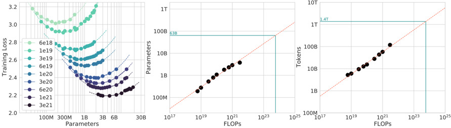Approach 2: IsoFLOP profiles In our second approach we vary the model size 5 for a fixed set of 9 different training FLOP counts 6 (ranging from 6 10 18 to 3 10 21 FLOPs), and consider the final training loss for each point 7 . in contrast with Approach 1 that considered points ' 𝑁 𝐷 𝐿 ' along the entire training runs. This allows us to directly answer the question: For a given FLOP budget, what is the optimal parameter count? 4 Note that all selected points are within the last 15% of training. This suggests that when training a model over 𝐷 tokens, we should pick a cosine cycle length that decays 10 over approximately 𝐷 tokens-see further details in Appendix B. 5 In approach 2, model size varies up to 16B as opposed to approach 1 where we only used models up to 10B. 6 The number of training tokens is determined by the model size and training FLOPs. 7 We set the cosine schedule length to match the number of tokens, which is optimal according to the analysis presented in Appendix B. Figure 3 j IsoFLOP curves. For various model sizes, we choose the number of training tokens such that the final FLOPs is a constant. The cosine cycle length is set to match the target FLOP count. We find a clear valley in loss, meaning that for a given FLOP budget there is an optimal model to train ( left ). Using the location of these valleys, we project optimal model size and number of tokens for larger models ( center and right ). In green, we show the estimated number of parameters and tokens for an optimal model trained with the compute budget of Gopher . <details> <summary>Image 4 Details</summary>  ### Visual Description ## Chart Type: Multi-Panel Chart ### Overview The image presents a multi-panel chart consisting of three sub-charts. The first chart (left) shows the relationship between "Training Loss" and "Parameters" for different model sizes. The second chart (middle) shows the relationship between "Parameters" and "FLOPs". The third chart (right) shows the relationship between "Tokens" and "FLOPs". All charts use logarithmic scales on both axes. ### Components/Axes **Left Chart:** * **X-axis:** Parameters (log scale), labeled with 100M, 300M, 1B, 3B, 6B, 30B * **Y-axis:** Training Loss (linear scale), labeled from 2.0 to 3.2 in increments of 0.2. * **Legend:** Located in the middle-left of the chart. The legend entries are: * 6e18 (light green) * 1e19 (green) * 3e19 (teal) * 6e19 (dark teal) * 1e20 (blue) * 3e20 (dark blue) * 6e20 (purple) * 1e21 (dark purple) * 3e21 (black) **Middle Chart:** * **X-axis:** FLOPs (log scale), labeled with 10^17, 10^19, 10^21, 10^23, 10^25 * **Y-axis:** Parameters (log scale), labeled with 100M, 1B, 10B, 100B, 1T * A horizontal teal line extends from the y-axis at 63B. * A dashed red line extends diagonally from the bottom left to the top right. **Right Chart:** * **X-axis:** FLOPs (log scale), labeled with 10^17, 10^19, 10^21, 10^23, 10^25 * **Y-axis:** Tokens (log scale), labeled with 100M, 1B, 10B, 100B, 1T, 10T * A horizontal teal line extends from the y-axis at 1.4T. * A dashed red line extends diagonally from the bottom left to the top right. ### Detailed Analysis **Left Chart:** Each line represents a different model size (parameter count). The x-axis represents the number of parameters, and the y-axis represents the training loss. Each line shows a U-shaped curve, indicating that there is an optimal number of parameters for minimizing training loss for each model size. * **6e18 (light green):** The line starts at approximately (100M, 3.1), decreases to a minimum around (300M, 2.9), and then increases to approximately (6B, 3.1). * **1e19 (green):** The line starts at approximately (100M, 2.9), decreases to a minimum around (300M, 2.7), and then increases to approximately (6B, 2.9). * **3e19 (teal):** The line starts at approximately (100M, 2.7), decreases to a minimum around (300M, 2.5), and then increases to approximately (6B, 2.7). * **6e19 (dark teal):** The line starts at approximately (100M, 2.6), decreases to a minimum around (300M, 2.4), and then increases to approximately (6B, 2.6). * **1e20 (blue):** The line starts at approximately (100M, 2.5), decreases to a minimum around (300M, 2.3), and then increases to approximately (6B, 2.5). * **3e20 (dark blue):** The line starts at approximately (100M, 2.4), decreases to a minimum around (300M, 2.25), and then increases to approximately (6B, 2.4). * **6e20 (purple):** The line starts at approximately (100M, 2.3), decreases to a minimum around (300M, 2.2), and then increases to approximately (6B, 2.3). * **1e21 (dark purple):** The line starts at approximately (100M, 2.25), decreases to a minimum around (300M, 2.15), and then increases to approximately (6B, 2.25). * **3e21 (black):** The line starts at approximately (100M, 2.2), decreases to a minimum around (300M, 2.1), and then increases to approximately (6B, 2.2). **Middle Chart:** The black dots represent data points showing the relationship between the number of parameters and the number of FLOPs. The data points generally follow a linear trend on the log-log scale, indicating a power-law relationship. The teal line intersects the data points at approximately 63B parameters and 10^23 FLOPs. The red dashed line represents a 1:1 relationship. * The data points are approximately: (10^18, 200M), (10^19, 500M), (10^20, 2B), (10^21, 10B), (10^22, 50B), (10^23, 63B) **Right Chart:** The black dots represent data points showing the relationship between the number of tokens and the number of FLOPs. The data points generally follow a linear trend on the log-log scale, indicating a power-law relationship. The teal line intersects the data points at approximately 1.4T tokens and 10^23 FLOPs. The red dashed line represents a 1:1 relationship. * The data points are approximately: (10^18, 200M), (10^19, 500M), (10^20, 2B), (10^21, 10B), (10^22, 50B), (10^23, 1.4T) ### Key Observations * **Left Chart:** As the model size increases, the minimum training loss decreases, but the curves become flatter. * **Middle Chart:** There is a strong correlation between the number of parameters and the number of FLOPs. * **Right Chart:** There is a strong correlation between the number of tokens and the number of FLOPs. * The teal lines in the middle and right charts indicate a specific FLOPs value (around 10^23) and the corresponding parameter count (63B) and token count (1.4T). ### Interpretation The charts suggest that increasing model size (number of parameters) initially leads to a decrease in training loss, but there are diminishing returns. The middle and right charts indicate that the number of parameters and the number of tokens are both strongly correlated with the number of FLOPs. The teal lines highlight a specific point where a certain number of FLOPs corresponds to a particular number of parameters and tokens. This information can be used to optimize model training and resource allocation. The red dashed lines show the point where the x and y axis are equal. </details> For each FLOP budget, we plot the final loss (after smoothing) against the parameter count in Figure 3 (left). In all cases, we ensure that we have trained a diverse enough set of model sizes to see a clear minimum in the loss. We fit a parabola to each IsoFLOPs curve to directly estimate at what model size the minimum loss is achieved (Figure 3 (left)). As with the previous approach, we then fit a power law between FLOPs and loss-optimal model size and number of training tokens, shown in Figure 3 (center, right). Again, we fit exponents of the form 𝑁𝑜𝑝𝑡 / 𝐶 𝑎 and 𝐷𝑜𝑝𝑡 / 𝐶 𝑏 and we find that 𝑎 = 0 49 and 𝑏 = 0 51-as summarized in Table 2. ## 3.3. Approach 3: Fitting a parametric loss function Lastly, we model all final losses from experiments in Approach 1 & 2 as a parametric function of model parameter count and the number of seen tokens. Following a classical risk decomposition (see Section D.2), we propose the following functional form <!-- formula-not-decoded --> The first term captures the loss for an ideal generative process on the data distribution, and should correspond to the entropy of natural text. The second term captures the fact that a perfectly trained transformer with 𝑁 parameters underperforms the ideal generative process. The final term captures the fact that the transformer is not trained to convergence, as we only make a finite number of optimisation steps, on a sample of the dataset distribution. Model fitting. To estimate ' 𝐴 𝐵 𝐸 𝛼 𝛽 ' , we minimize the Huber loss (Huber, 1964) between the predicted and observed log loss using the L-BFGS algorithm (Nocedal, 1980): <!-- formula-not-decoded --> We account for possible local minima by selecting the best fit from a grid of initialisations. The Huber loss ( 𝛿 = 10 3 ) is robust to outliers, which we find important for good predictive performance over held-out data points. Section D.2 details the fitting procedure and the loss decomposition. 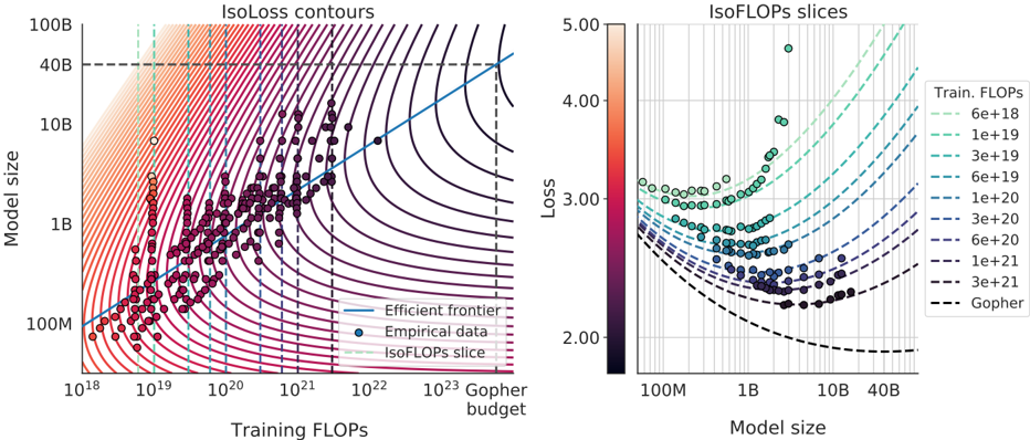Figure 4 j Parametric fit. We fit a parametric modelling of the loss ˆ 𝐿 ' 𝑁 𝐷 ' and display contour ( left ) and isoFLOP slices ( right ). For each isoFLOP slice, we include a corresponding dashed line in the left plot. In the left plot, we show the efficient frontier in blue, which is a line in log-log space. Specifically , the curve goes through each iso-loss contour at the point with the fewest FLOPs. We project the optimal model size given the Gopher FLOP budget to be 40B parameters. <details> <summary>Image 5 Details</summary>  ### Visual Description ## Chart: IsoLoss Contours and IsoFLOPs Slices ### Overview The image presents two related charts. The left chart, titled "IsoLoss contours," plots model size against training FLOPS, displaying contours of constant loss and empirical data points. The right chart, titled "IsoFLOPs slices," plots loss against model size, showing slices of constant training FLOPS. Both charts aim to visualize the relationship between model size, training FLOPS, and loss. ### Components/Axes **Left Chart: IsoLoss contours** * **Title:** IsoLoss contours * **X-axis:** Training FLOPS (log scale), with markers at 10^18, 10^19, 10^20, 10^21, 10^22, and 10^23, labeled "Gopher budget". * **Y-axis:** Model size (log scale), with markers at 100M, 1B, 10B, 40B, and 100B. * **Contours:** IsoLoss contours are represented by curved lines. The color gradient suggests that contours closer to the bottom-left represent lower loss values. * **Data Points:** Empirical data is plotted as dots. The color of the dots varies, likely representing a third dimension (possibly loss or training FLOPS). * **Efficient Frontier:** A blue line represents the efficient frontier. * **IsoFLOPs slice:** Vertical dashed lines represent IsoFLOPs slices. **Right Chart: IsoFLOPs slices** * **Title:** IsoFLOPs slices * **X-axis:** Model size (log scale), with markers at 100M, 1B, 10B, and 40B. * **Y-axis:** Loss (linear scale), with markers at 2.00, 3.00, 4.00, and 5.00. * **Data Points:** Empirical data is plotted as dots. The color of the dots varies from red to green, likely representing a third dimension (possibly loss or training FLOPS). * **IsoFLOPs slices:** Dashed lines represent IsoFLOPs slices. * **Legend (Top Right):** * 6e+18 (light green dashed line) * 1e+19 (green dashed line) * 3e+19 (green dashed line) * 6e+19 (blue-green dashed line) * 1e+20 (blue dashed line) * 3e+20 (blue dashed line) * 6e+20 (dark blue dashed line) * 1e+21 (dark blue dashed line) * 3e+21 (black dashed line) * Gopher (black dashed line) **Legend (Bottom Left of Left Chart):** * Efficient frontier (blue line) * Empirical data (blue dot) * IsoFLOPs slice (light green dashed line) ### Detailed Analysis **Left Chart: IsoLoss contours** * The empirical data points are clustered in the lower-right region of the chart, indicating a trend towards larger models and higher training FLOPS. * The efficient frontier (blue line) appears to represent the optimal trade-off between model size and training FLOPS for a given loss. * The IsoLoss contours show that as you move towards the top-right of the chart (larger models and more training FLOPS), the loss decreases. * The vertical dashed lines (IsoFLOPs slices) are spaced unevenly, with closer spacing on the left side of the chart. **Right Chart: IsoFLOPs slices** * The IsoFLOPs slices generally show a U-shaped curve, indicating that there is an optimal model size for a given training FLOPS that minimizes loss. * The minimum loss for each IsoFLOPs slice shifts to the right (larger model sizes) as the training FLOPS increases. * The data points are clustered around the minimum loss points of the IsoFLOPs slices. * The color of the data points varies from red (lower left) to green (upper right), suggesting that higher training FLOPS are associated with lower loss. ### Key Observations * There is a clear trade-off between model size, training FLOPS, and loss. * Larger models and more training FLOPS generally lead to lower loss, but there are diminishing returns. * The efficient frontier represents the optimal trade-off between model size and training FLOPS. * The IsoFLOPs slices show that there is an optimal model size for a given training FLOPS. ### Interpretation The charts illustrate the relationship between model size, training FLOPS, and loss in machine learning models. The IsoLoss contours show the overall trend that larger models and more training FLOPS lead to lower loss. However, the IsoFLOPs slices reveal that for a fixed amount of training FLOPS, there is an optimal model size that minimizes loss. This suggests that simply increasing model size or training FLOPS indefinitely is not the most efficient way to improve model performance. The efficient frontier represents the best possible trade-off between model size and training FLOPS for a given loss, and it can be used to guide the selection of model architectures and training strategies. The empirical data points provide real-world examples of model performance and can be used to validate the theoretical relationships shown in the charts. The "Gopher budget" line on the left chart likely represents a constraint on the available training FLOPS, and it can be used to determine the optimal model size for a given budget. </details> Efficient frontier. We can approximate the functions 𝑁𝑜𝑝𝑡 and 𝐷𝑜𝑝𝑡 by minimizing the parametric loss ˆ 𝐿 under the constraint FLOPs ' 𝑁 𝐷 ' 6 𝑁𝐷 (Kaplan et al., 2020). The resulting 𝑁𝑜𝑝𝑡 and 𝐷𝑜𝑝𝑡 balance the two terms in Equation (3) that depend on model size and data. By construction, they have a power-law form: <!-- formula-not-decoded --> Weshow contours of the fitted function ˆ 𝐿 in Figure 4 (left), and the closed-form efficient computational frontier in blue. From this approach, we find that 𝑎 = 0 46 and 𝑏 = 0 54-as summarized in Table 2. ## 3.4. Optimal model scaling We find that the three approaches, despite using different fitting methodologies and different trained models, yield comparable predictions for the optimal scaling in parameters and tokens with FLOPs (shown in Table 2). All three approaches suggest that as compute budget increases, model size and the amount of training data should be increased in approximately equal proportions. The first and second approaches yield very similar predictions for optimal model sizes, as shown in Figure 1 and Figure A3. The third approach predicts even smaller models being optimal at larger compute budgets. We note that the observed points ' 𝐿 𝑁 𝐷 ' for low training FLOPs ( 𝐶 6 1 𝑒 21) have larger residuals k 𝐿 ˆ 𝐿 ' 𝑁 𝐷 'k 2 2 than points with higher computational budgets. The fitted model places increased weight on the points with more FLOPs-automatically considering the low-computational budget points as outliers due to the Huber loss. As a consequence of the empirically observed negative curvature in the frontier 𝐶 ! 𝑁𝑜𝑝𝑡 (see Appendix E), this results in predicting a lower 𝑁𝑜𝑝𝑡 than the two other approaches. In Table 3 we show the estimated number of FLOPs and tokens that would ensure that a model of a given size lies on the compute-optimal frontier. Our findings suggests that the current generation of Table 2 j Estimated parameter and data scaling with increased training compute. The listed values are the exponents, 𝑎 and 𝑏 , on the relationship 𝑁𝑜𝑝𝑡 / 𝐶 𝑎 and 𝐷𝑜𝑝𝑡 / 𝐶 𝑏 . Our analysis suggests a near equal scaling in parameters and data with increasing compute which is in clear contrast to previous work on the scaling of large models. The 10 th and 90 th percentiles are estimated via bootstrapping data (80% of the dataset is sampled 100 times) and are shown in parenthesis. | Approach | Coeff. 𝑎 where 𝑁 𝑜𝑝𝑡 / 𝐶 𝑎 | Coeff. 𝑏 where 𝐷 𝑜𝑝𝑡 / 𝐶 𝑏 | |-------------------------------------|------------------------------------------------------------------|------------------------------------------------------------------| | 1. Minimum over training curves | 0 50 ' 0 488 0 502 ' | 0 50 ' 0 501 0 512 ' | | 2. IsoFLOP profiles | 0 49 ' 0 462 0 534 ' | 0 51 ' 0 483 0 529 ' | | 3. Parametric modelling of the loss | 0 46 ' 0 454 0 455 ' | 0 54 ' 0 542 0 543 ' | | Kaplan et al. (2020) | 0.73 | 0.27 | Table 3 j Estimated optimal training FLOPs and training tokens for various model sizes. For various model sizes, we show the projections from Approach 1 of how many FLOPs and training tokens would be needed to train compute-optimal models. The estimates for Approach 2 & 3 are similar (shown in Section D.3) . | Parameters | FLOPs | FLOPs (in Gopher unit) | Tokens | |--------------|----------|--------------------------------|----------------| | 400 Million | 1.92e+19 | 1 29 968 | 8.0 Billion | | 1 Billion | 1.21e+20 | 1 4 761 | 20.2 Billion | | 10 Billion | 1.23e+22 | 1 46 | 205.1 Billion | | 67 Billion | 5.76e+23 | 1 | 1.5 Trillion | | 175 Billion | 3.85e+24 | 6 7 | 3.7 Trillion | | 280 Billion | 9.9e+24 | 17 2 | 5.9 Trillion | | 520 Billion | 3.43e+25 | 59 5 | 11.0 Trillion | | 1 Trillion | 1.27e+26 | 221 3 | 21.2 Trillion | | 10 Trillion | 1.3e+28 | 22515 9 | 216.2 Trillion | large language models are considerably over-sized, given their respective compute budgets, as shown in Figure 1. For example, we find that a 175 billion parameter model should be trained with a compute budget of 4 41 10 24 FLOPs and on over 4.2 trillion tokens. A 280 billion Gopher -like model is the optimal model to train given a compute budget of approximately 10 25 FLOPs and should be trained on 6.8 trillion tokens. Unless one has a compute budget of 10 26 FLOPs (over 250 the compute used to train Gopher ), a 1 trillion parameter model is unlikely to be the optimal model to train. Furthermore, the amount of training data that is projected to be needed is far beyond what is currently used to train large models, and underscores the importance of dataset collection in addition to engineering improvements that allow for model scale. While there is significant uncertainty extrapolating out many orders of magnitude, our analysis clearly suggests that given the training compute budget for many current LLMs, smaller models should have been trained on more tokens to achieve the most performant model. In Appendix C, we reproduce the IsoFLOP analysis on two additional datasets: C4 (Raffel et al., 2020a) and GitHub code (Rae et al., 2021). In both cases we reach the similar conclusion that model size and number of training tokens should be scaled in equal proportions. ## 4. Chinchilla Based on our analysis in Section 3, the optimal model size for the Gopher compute budget is somewhere between 40 and 70 billion parameters. We test this hypothesis by training a model on the larger end of this range-70B parameters-for 1.4T tokens, due to both dataset and computational efficiency considerations. In this section we compare this model, which we call Chinchilla , to Gopher and other LLMs. Both Chinchilla and Gopher have been trained for the same number of FLOPs but differ in the size of the model and the number of training tokens. While pre-training a large language model has a considerable compute cost, downstream finetuning and inference also make up substantial compute usage (Rae et al., 2021). Due to being 4 smaller than Gopher , both the memory footprint and inference cost of Chinchilla are also smaller. ## 4.1. Model and training details The full set of hyperparameters used to train Chinchilla are given in Table 4. Chinchilla uses the same model architecture and training setup as Gopher with the exception of the differences listed below. - We train Chinchilla on MassiveText (the same dataset as Gopher ) but use a slightly different subset distribution (shown in Table A1) to account for the increased number of training tokens. - We train Chinchilla with a slightly modified SentencePiece (Kudo and Richardson, 2018) tokenizer that does not apply NFKC normalisation. The vocabulary is very similar- 94.15% of tokens are the same as those used for training Gopher . We find that this particularly helps with the representation of mathematics and chemistry, for example. - We use AdamW (Loshchilov and Hutter, 2019) for Chinchilla rather than Adam (Kingma and Ba, 2014) as this improves the language modelling loss and the downstream task performance after finetuning. 8 - Whilst the forward and backward pass are computed in bfloat16 , we store a float32 copy of the weights in the distributed optimiser state (Rajbhandari et al., 2020). See Lessons Learned from Rae et al. (2021) for additional details. In Appendix G we show the impact of the various optimiser related changes between Chinchilla and Gopher . All models in this analysis have been trained on TPUv3/TPUv4 (Jouppi et al., 2017) with JAX (Bradbury et al., 2018) and Haiku (Hennigan et al., 2020). We include a Chinchilla model card (Mitchell et al., 2019) in Table A8. | Model | Layers | Number Heads | Key/Value Size | d model | Max LR | Batch Size | |----------------|----------|----------------|------------------|-----------|--------------------------|--------------| | Gopher 280B | 80 | 128 | 128 | 16,384 | 4 10 5 | 3M ! 6M | | Chinchilla 70B | 80 | 64 | 128 | 8,192 | 1 10 4 | 1.5M ! 3M | Table 4 j Chinchilla architecture details. We list the number of layers, the key/value size, the bottleneck activation size d model , the maximum learning rate, and the training batch size (# tokens). The feed-forward size is always set to 4 dmodel . Note that we double the batch size midway through training for both Chinchilla and Gopher . 8 Interestingly , a model trained with AdamW only passes the training performance of a model trained with Adam around 80% of the way through the cosine cycle, though the ending performance is notably better- see Figure A7 Table 5 j All evaluation tasks. We evaluate Chinchilla on a collection of language modelling along with downstream tasks. We evaluate on largely the same tasks as in Rae et al. (2021), to allow for direct comparison. | | # Tasks | Examples | |-----------------------|-----------|---------------------------------------------------------------------------------------------| | Language Modelling | 20 | WikiText-103, The Pile: PG-19, arXiv, FreeLaw, | | Reading Comprehension | 3 | RACE-m, RACE-h, LAMBADA | | Question Answering | 3 | Natural Questions, TriviaQA, TruthfulQA | | Common Sense | 5 | HellaSwag, Winogrande, PIQA, SIQA, BoolQ | | MMLU | 57 | High School Chemistry, Astronomy, Clinical Knowledge, | | BIG-bench | 62 | Causal Judgement, Epistemic Reasoning, Temporal Sequences, | ## 4.2. Results We perform an extensive evaluation of Chinchilla , comparing against various large language models. We evaluate on a large subset of the tasks presented in Rae et al. (2021), shown in Table 5. As the focus of this work is on optimal model scaling, we included a large representative subset, and introduce a few new evaluations to allow for better comparison to other existing large models. The evaluation details for all tasks are the same as described in Rae et al. (2021). ## 4.2.1. 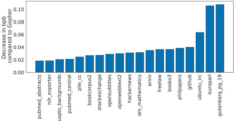Language modelling Figure 5 j Pile Evaluation. For the different evaluation sets in The Pile (Gao et al., 2020), we show the bits-per-byte (bpb) improvement (decrease) of Chinchilla compared to Gopher . On all subsets, Chinchilla outperforms Gopher . <details> <summary>Image 6 Details</summary>  ### Visual Description ## Bar Chart: Decrease in bpb Compared to Gopher ### Overview The image is a bar chart comparing the decrease in bits per byte (bpb) relative to Gopher for various datasets. The x-axis represents different datasets, and the y-axis represents the decrease in bpb compared to Gopher. The bars are all blue. ### Components/Axes * **X-axis:** Datasets (pubmed\_abstracts, nih\_exporter, uspto\_backgrounds, pubmed\_central, pile\_cc, bookcorpus2, stackexchange, opensubtitles, openwebtext2, hackernews, dm\_mathematics, arxiv, freelaw, books3, philpapers, github, ubuntu\_irc, europarl, gutenberg\_pg\_19) * **Y-axis:** Decrease in bpb compared to Gopher, ranging from 0.00 to 0.10 with increments of 0.02. ### Detailed Analysis The bar chart shows the decrease in bits per byte (bpb) compared to Gopher for different datasets. The datasets are arranged in ascending order of decrease in bpb. Here's a breakdown of the approximate values for each dataset: * pubmed\_abstracts: ~0.018 * nih\_exporter: ~0.019 * uspto\_backgrounds: ~0.021 * pubmed\_central: ~0.022 * pile\_cc: ~0.025 * bookcorpus2: ~0.027 * stackexchange: ~0.028 * opensubtitles: ~0.029 * openwebtext2: ~0.031 * hackernews: ~0.032 * dm\_mathematics: ~0.033 * arxiv: ~0.035 * freelaw: ~0.036 * books3: ~0.036 * philpapers: ~0.039 * github: ~0.040 * ubuntu\_irc: ~0.063 * europarl: ~0.102 * gutenberg\_pg\_19: ~0.105 The general trend is an upward slope, indicating an increasing decrease in bpb compared to Gopher as we move from left to right along the x-axis. ### Key Observations * The datasets 'europarl' and 'gutenberg\_pg\_19' show the most significant decrease in bpb compared to Gopher. * The datasets 'pubmed\_abstracts', 'nih\_exporter', 'uspto\_backgrounds', and 'pubmed\_central' show the least decrease in bpb compared to Gopher. * There is a noticeable jump in the decrease in bpb between 'github' and 'ubuntu\_irc'. ### Interpretation The bar chart illustrates the relative compression efficiency of different datasets compared to Gopher. A higher bar indicates a greater reduction in bits per byte when using a different compression method (presumably a more modern one) compared to Gopher. The 'europarl' and 'gutenberg\_pg\_19' datasets benefit the most from the alternative compression, suggesting they contain patterns or redundancies that Gopher struggles to exploit. Conversely, 'pubmed\_abstracts' and similar datasets show only a marginal improvement, implying they are already relatively well-compressed or lack the types of redundancies that the newer compression methods can effectively address. The jump between 'github' and 'ubuntu\_irc' suggests a significant difference in the compressibility characteristics of these two types of data. </details> Chinchilla significantly outperforms Gopher on all evaluation subsets of The Pile (Gao et al., 2020), as shown in Figure 5. Compared to Jurassic-1 (178B) Lieber et al. (2021), Chinchilla is more performant on all but two subsets-dm\_mathematics and ubuntu\_irc - see Table A5 for a raw bits-per-byte comparison. On Wikitext103 (Merity et al., 2017), Chinchilla achieves a perplexity of 7.16 compared to 7.75 for Gopher . Some caution is needed when comparing Chinchilla with Gopher on these language modelling benchmarks as Chinchilla is trained on 4 more data than Gopher and thus train/test set leakage may artificially enhance the results. We thus place more emphasis on other Table 6 j Massive Multitask Language Understanding (MMLU). We report the average 5-shot accuracy over 57 tasks with model and human accuracy comparisons taken from Hendrycks et al. (2020). We also include the average prediction for state of the art accuracy in June 2022/2023 made by 73 competitive human forecasters in Steinhardt (2021). | Random | 25.0% | |----------------------------------|---------| | Average human rater | 34.5% | | GPT-3 5-shot | 43.9% | | Gopher 5-shot | 60.0% | | Chinchilla 5-shot | 67.6% | | Average human expert performance | 89.8% | | June 2022 Forecast | 57.1% | | June 2023 Forecast | 63.4% | tasks for which leakage is less of a concern, such as MMLU (Hendrycks et al., 2020) and BIG-bench (BIG-bench collaboration, 2021) along with various closed-book question answering and common sense analyses. ## 4.2.2. MMLU The Massive Multitask Language Understanding (MMLU) benchmark (Hendrycks et al., 2020) consists of a range of exam-like questions on academic subjects. In Table 6, we report Chinchilla 's average 5-shot performance on MMLU (the full breakdown of results is shown in Table A6). On this benchmark, Chinchilla significantly outperforms Gopher despite being much smaller, with an average accuracy of 67.6% (improving upon Gopher by 7.6%). Remarkably, Chinchilla even outperforms the expert forecast for June 2023 of 63.4% accuracy (see Table 6) (Steinhardt, 2021). Furthermore, Chinchilla achieves greater than 90% accuracy on 4 different individual tasks-high\_school\_gov\_and\_politics, international\_law, sociology , and us\_foreign\_policy . To our knowledge, no other model has achieved greater than 90% accuracy on a subset. 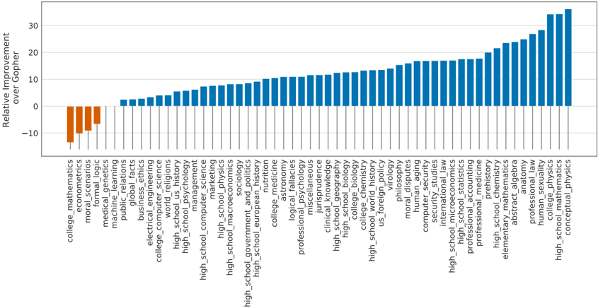In Figure 6, we show a comparison to Gopher broken down by task. Overall, we find that Chinchilla improves performance on the vast majority of tasks. On four tasks ( college\_mathematics, econometrics, moral\_scenarios , and formal\_logic ) Chinchilla underperforms Gopher , and there is no change in performance on two tasks. ## 4.2.3. Reading comprehension On the final word prediction dataset LAMBADA (Paperno et al., 2016), Chinchilla achieves 77.4% accuracy, compared to 74.5% accuracy from Gopher and 76.6% from MT-NLG 530B (see Table 7). On RACE-h and RACE-m (Lai et al., 2017), Chinchilla greatly outperforms Gopher , improving accuracy by more than 10% in both cases-see Table 7. ## 4.2.4. 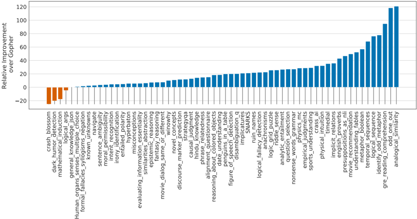BIG-bench We analysed Chinchilla on the same set of BIG-bench tasks (BIG-bench collaboration, 2021) reported in Rae et al. (2021). Similar to what we observed in MMLU, Chinchilla outperforms Gopher on the vast majority of tasks (see Figure 7). We find that Chinchilla improves the average performance by 10.7%, reaching an accuracy of 65.1% versus 54.4% for Gopher . Of the 62 tasks we consider, Chinchilla performs worse than Gopher on only four-crash\_blossom, dark\_humor\_detection, Figure 6 j MMLU results compared to Gopher We find that Chinchilla outperforms Gopher by 7.6% on average (see Table 6) in addition to performing better on 51/57 individual tasks, the same on 2/57, and worse on only 4/57 tasks. <details> <summary>Image 7 Details</summary>  ### Visual Description ## Bar Chart: Relative Improvement over Gopher ### Overview The image is a bar chart comparing the relative improvement of a system (unspecified) over a baseline system called "Gopher" across various subjects. The y-axis represents the relative improvement, while the x-axis lists the subjects. The bars are colored either blue (positive improvement) or orange (negative improvement). ### Components/Axes * **Y-axis:** "Relative Improvement over Gopher". The scale ranges from -10 to 30, with tick marks at -10, 0, 10, 20, and 30. * **X-axis:** Categorical axis listing various subjects. The labels are rotated vertically to fit. * **Bar Colors:** * Blue: Indicates a positive relative improvement over Gopher. * Orange: Indicates a negative relative improvement over Gopher. ### Detailed Analysis The chart displays the relative improvement over Gopher for a range of subjects. The subjects are listed along the x-axis, and the corresponding bar height indicates the magnitude of the improvement or decline. Here's a breakdown of the data, starting from the left: * **Negative Improvement (Orange Bars):** * college_mathematics: Approximately -12 * econometrics: Approximately -9 * moral_scenarios: Approximately -8 * formal_logic: Approximately -6 * medical_genetics: Approximately -4 * **Positive Improvement (Blue Bars):** * machine_learning: Approximately 2 * public_relations: Approximately 3 * global_facts: Approximately 3 * business_ethics: Approximately 3 * electrical_engineering: Approximately 4 * college_computer_science: Approximately 4 * world_religions: Approximately 5 * high_school_us_history: Approximately 6 * high_school_psychology: Approximately 6 * management: Approximately 6 * high_school_computer_science: Approximately 7 * marketing: Approximately 7 * high_school_physics: Approximately 8 * high_school_macroeconomics: Approximately 8 * sociology: Approximately 9 * high_school_government_and_politics: Approximately 9 * high_school_european_history: Approximately 9 * nutrition: Approximately 10 * college_medicine: Approximately 11 * astronomy: Approximately 11 * logical_fallacies: Approximately 12 * professional_psychology: Approximately 12 * miscellaneous: Approximately 13 * jurisprudence: Approximately 13 * clinical_knowledge: Approximately 14 * high_school_geography: Approximately 14 * high_school_biology: Approximately 15 * college_biology: Approximately 15 * college_chemistry: Approximately 16 * high_school_world_history: Approximately 16 * us_foreign_policy: Approximately 17 * virology: Approximately 17 * philosophy: Approximately 18 * moral_disputes: Approximately 18 * human_aging: Approximately 19 * computer_security: Approximately 19 * security_studies: Approximately 20 * international_law: Approximately 20 * high_school_microeconomics: Approximately 21 * high_school_statistics: Approximately 21 * professional_accounting: Approximately 22 * professional_medicine: Approximately 22 * prehistory: Approximately 23 * high_school_chemistry: Approximately 23 * elementary_mathematics: Approximately 24 * abstract_algebra: Approximately 24 * anatomy: Approximately 25 * professional_law: Approximately 26 * human_sexuality: Approximately 27 * college_physics: Approximately 28 * high_school_mathematics: Approximately 30 * conceptual_physics: Approximately 32 ### Key Observations * The majority of subjects show a positive relative improvement over Gopher. * College mathematics shows the largest negative relative improvement. * Conceptual physics shows the largest positive relative improvement. * There is a wide range of performance across different subjects. ### Interpretation The bar chart indicates that the system being evaluated generally outperforms the "Gopher" baseline across a variety of subjects. However, there are some subjects, particularly in college mathematics, where the system performs worse than Gopher. The substantial positive improvement in areas like conceptual physics and high school mathematics suggests that the system may be particularly well-suited for these domains. The data suggests that the system's strengths and weaknesses are subject-dependent, and further investigation may be warranted to understand the underlying reasons for these differences in performance. </details> Table 7 j Reading comprehension. On RACE-h and RACE-m (Lai et al., 2017), Chinchilla considerably improves performance over Gopher . Note that GPT-3 and MT-NLG 530B use a different prompt format than we do on RACE-h/m, so results are not comparable to Gopher and Chinchilla . On LAMBADA (Paperno et al., 2016), Chinchilla outperforms both Gopher and MT-NLG 530B. | | Chinchilla | Gopher | GPT-3 | MT-NLG 530B | |-------------------|--------------|----------|---------|---------------| | LAMBADA Zero-Shot | 77.4 | 74.5 | 76.2 | 76.6 | | RACE-m Few-Shot | 86.8 | 75.1 | 58.1 | - | | RACE-h Few-Shot | 82.3 | 71.6 | 46.8 | 47.9 | mathematical\_induction and logical\_args . Full accuracy results for Chinchilla can be found in Table A7. ## 4.2.5. Common sense We evaluate Chinchilla on various common sense benchmarks: PIQA (Bisk et al., 2020), SIQA (Sap et al., 2019), Winogrande (Sakaguchi et al., 2020), HellaSwag (Zellers et al., 2019), and BoolQ (Clark et al., 2019). We find that Chinchilla outperforms both Gopher and GPT-3 on all tasks and outperforms MT-NLG 530B on all but one task-see Table 8. On TruthfulQA (Lin et al., 2021), Chinchilla reaches 43.6%, 58.5%, and 66.7% accuracy with 0-shot, 5-shot, and 10-shot respectively. In comparison, Gopher achieved only 29.5% 0-shot and 43.7% 10-shot accuracy. In stark contrast with the findings of Lin et al. (2021), the large improvements (14.1% in 0-shot accuracy) achieved by Chinchilla suggest that better modelling of the pre-training data alone can lead to substantial improvements on this benchmark. Figure 7 j BIG-bench results compared to Gopher Chinchilla out performs Gopher on all but four BIG-bench tasks considered. Full results are in Table A7. <details> <summary>Image 8 Details</summary>  ### Visual Description ## Bar Chart: Relative Improvement over Gopher ### Overview The image is a bar chart comparing the relative improvement of a system over "Gopher" across a range of tasks. The x-axis represents different tasks, and the y-axis represents the relative improvement, with both positive and negative values. The bars are colored blue for positive improvement and orange for negative improvement. ### Components/Axes * **Y-axis:** "Relative Improvement over Gopher". The scale ranges from -20 to 120, with increments of 20. * **X-axis:** Categorical axis listing various tasks or categories. The labels are rotated for readability. * **Bar Colors:** * Blue: Indicates a positive relative improvement over Gopher. * Orange: Indicates a negative relative improvement over Gopher. ### Detailed Analysis The chart displays the relative performance across a variety of tasks. The tasks are listed along the x-axis, and the relative improvement over Gopher is shown on the y-axis. Here's a breakdown of the data, starting from the left: * **Negative Improvement (Orange Bars):** * crash_blossom: Approximately -25 * dark_humor_detection: Approximately -18 * mathematical_induction: Approximately -15 * logical_args: Approximately -5 * **Positive Improvement (Blue Bars):** * general_knowledge_json: Approximately 2 * Human_organs_senses_multiple_choice: Approximately 2 * formal_fallacies_syllogisms_negation: Approximately 2 * known_unknowns: Approximately 3 * navigate: Approximately 3 * sentence_ambiguity: Approximately 3 * moral_permissibility: Approximately 3 * intent_recognition: Approximately 3 * irony_identification: Approximately 3 * entailed_polarity: Approximately 4 * hyperbaton: Approximately 4 * misconceptions: Approximately 4 * evaluating_information_essentiality: Approximately 4 * similarities_abstraction: Approximately 4 * epistemic_reasoning: Approximately 4 * fantasy_reasoning: Approximately 4 * movie_dialog_same_or_different: Approximately 4 * winowhy: Approximately 4 * novel_concepts: Approximately 4 * discourse_marker_prediction: Approximately 4 * strategyqa: Approximately 4 * causal_judgment: Approximately 4 * hindu_knowledge: Approximately 4 * phrase_relatedness: Approximately 4 * alignment_questionnaire: Approximately 4 * reasoning_about_colored_objects: Approximately 4 * date_understanding: Approximately 4 * penguins_in_a_table: Approximately 4 * figure_of_speech_detection: Approximately 4 * disambiguation_q: Approximately 4 * implicatures: Approximately 4 * SNARKS: Approximately 4 * ruin_names: Approximately 4 * logical_fallacy_detection: Approximately 4 * anachronisms: Approximately 4 * logic_grid_puzzle: Approximately 4 * riddle_sense: Approximately 4 * analytic_entailment: Approximately 4 * question_selection: Approximately 4 * nonsense_words_grammar: Approximately 5 * physics_mc: Approximately 5 * empirical_judgments: Approximately 5 * sports_understanding: Approximately 5 * crass_ai: Approximately 5 * physical_intuition: Approximately 6 * timedial: Approximately 6 * implicit_relations: Approximately 7 * english_proverbs: Approximately 10 * presuppositions_as_nli: Approximately 12 * movie_recommendation: Approximately 15 * understanding_fables: Approximately 20 * metaphor_boolean: Approximately 25 * temporal_sequences: Approximately 30 * logical_sequence: Approximately 35 * identify_odd_metaphor: Approximately 45 * gre_reading_comprehension: Approximately 60 * odd_one_out: Approximately 80 * analogical_similarity: Approximately 100 ### Key Observations * Most tasks show a positive relative improvement over Gopher. * "crash_blossom", "dark_humor_detection", "mathematical_induction", and "logical_args" show a negative relative improvement. * "analogical_similarity" shows the highest relative improvement. ### Interpretation The chart indicates that the system being evaluated generally outperforms Gopher across a wide range of tasks. However, it underperforms on tasks related to "crash_blossom", "dark_humor_detection", "mathematical_induction", and "logical_args". The significant outperformance on "analogical_similarity" and "odd_one_out" suggests a strength in these areas. The data suggests that the system has specific strengths and weaknesses compared to Gopher, which could be further investigated to understand the underlying reasons for these differences. </details> ## 4.2.6. Closed-book question answering Results on closed-book question answering benchmarks are reported in Table 9. On the Natural Questions dataset (Kwiatkowski et al., 2019), Chinchilla achieves new closed-book SOTA accuracies: 31.5% 5-shot and 35.5% 64-shot, compared to 21% and 28% respectively, for Gopher . On TriviaQA (Joshi et al., 2017) we show results for both the filtered (previously used in retrieval and open-book work) and unfiltered set (previously used in large language model evaluations). In both cases, Chinchilla substantially out performs Gopher . On the filtered version, Chinchilla lags behind the open book SOTA (Izacard and Grave, 2020) by only 7.9%. On the unfiltered set, Chinchilla outperforms GPT-3-see Table 9. ## 4.2.7. Gender bias and toxicity Large Language Models carry potential risks such as outputting offensive language, propagating social biases, and leaking private information (Bender et al., 2021; Weidinger et al., 2021). We expect Chinchilla to carry risks similar to Gopher because Chinchilla is trained on the same data, Table 8 j Zero-shot comparison on Common Sense benchmarks. We show a comparison between Chinchilla , Gopher , and MT-NLG 530B on various Common Sense benchmarks. We see that Chinchilla matches or outperforms Gopher and GPT-3 on all tasks. On all but one Chinchilla outperforms the much larger MT-NLG 530B model. | | Chinchilla | Gopher | GPT-3 | MT-NLG 530B | Supervised SOTA | |------------|--------------|----------|---------|---------------|-------------------| | HellaSWAG | 80.8% | 79.2% | 78.9% | 80.2% | 93.9% | | PIQA | 81.8% | 81.8% | 81.0% | 82.0% | 90.1% | | Winogrande | 74.9% | 70.1% | 70.2% | 73.0% | 91.3% | | SIQA | 51.3% | 50.6% | - | - | 83.2% | | BoolQ | 83.7 % | 79.3% | 60.5% | 78.2% | 91.4% | | | Method | Chinchilla | Gopher | GPT-3 | SOTA (open book) | |-----------------------------|-----------------------|-------------------|-------------------|---------------|--------------------| | Natural Questions (dev) | 0-shot 5-shot 64-shot | 16.6% 31.5% 35.5% | 10.1% 24.5% 28.2% | 14.6% - 29.9% | 54.4% | | TriviaQA (unfiltered, test) | 0-shot | 67.0% | 52.8% | 64.3% - | - | | | 5-shot 64-shot | 73.2% 72.3% | 63.6% | 71.2% | - | | | | 55.4% | 61.3% | | - | | TriviaQA (filtered, dev) | 0-shot | | 43.5% | - | 72.5% | | TriviaQA (filtered, dev) | 5-shot | 64.1% | 57.0% | - | 72.5% | | TriviaQA (filtered, dev) | 64-shot | 64.6% | 57.2% | - | 72.5% | Table 9 j Closed-book question answering. For Natural Questions (Kwiatkowski et al., 2019) and TriviaQA (Joshi et al., 2017), Chinchilla outperforms Gopher in all cases. On Natural Questions, Chinchilla outperforms GPT-3. On TriviaQA we show results on two different evaluation sets to allow for comparison to GPT-3 and to open book SOTA (FiD + Distillation (Izacard and Grave, 2020)). albeit with slightly different relative weights, and because it has a similar architecture. Here, we examine gender bias (particularly gender and occupation bias) and generation of toxic language. We select a few common evaluations to highlight potential issues, but stress that our evaluations are not comprehensive and much work remains to understand, evaluate, and mitigate risks in LLMs. Gender bias. As discussed in Rae et al. (2021), large language models reflect contemporary and historical discourse about different groups (such as gender groups) from their training dataset, and we expect the same to be true for Chinchilla . Here, we test if potential gender and occupation biases manifest in unfair outcomes on coreference resolutions, using the Winogender dataset (Rudinger et al., 2018) in a zero-shot setting. Winogender tests whether a model can correctly determine if a pronoun refers to different occupation words. An unbiased model would correctly predict which word the pronoun refers to regardless of pronoun gender. We follow the same setup as in Rae et al. (2021) (described further in Section H.3). As shown in Table 10, Chinchilla correctly resolves pronouns more frequently than Gopher across all groups. Interestingly, the performance increase is considerably smaller for male pronouns (increase of 3.2%) than for female or neutral pronouns (increases of 8.3% and 9.2% respectively). We also consider gotcha examples, in which the correct pronoun resolution contradicts gender stereotypes (determined by labor statistics). Again, we see that Chinchilla resolves pronouns more accurately than Gopher . When breaking up examples by male/female gender and gotcha / not gotcha , the largest improvement is on female gotcha examples (improvement of 10%). Thus, though Chinchilla uniformly overcomes gender stereotypes for more coreference examples than Gopher , the rate of improvement is higher for some pronouns than others, suggesting that the improvements conferred by using a more compute-optimal model can be uneven. Sample toxicity. Language models are capable of generating toxic language-including insults, hate speech, profanities and threats (Gehman et al., 2020; Rae et al., 2021). While toxicity is an umbrella term, and its evaluation in LMs comes with challenges (Welbl et al., 2021; Xu et al., 2021), automatic classifier scores can provide an indication for the levels of harmful text that a LM generates. Rae et al. (2021) found that improving language modelling loss by increasing the number of model parameters has only a negligible effect on toxic text generation (unprompted); here we analyze Table 10 j Winogender results. Left: Chinchilla consistently resolves pronouns better than Gopher . Right: Chinchilla performs better on examples which contradict gender stereotypes ( gotcha examples). However, difference in performance across groups suggests Chinchilla exhibits bias. | | Chinchilla | Gopher | | Chinchilla | Gopher | |---------|--------------|----------|-------------------|--------------|----------| | All | 78.3% | 71.4% | Male gotcha | 62.5% | 59.2% | | Male | 71.2% | 68.0% | Male not gotcha | 80.0% | 76.7% | | Female | 79.6% | 71.3% | Female gotcha | 76.7% | 66.7% | | Neutral | 84.2% | 75.0% | Female not gotcha | 82.5% | 75.8% | whether the same holds true for a lower LM loss achieved via more compute-optimal training. Similar to the protocol of Rae et al. (2021), we generate 25,000 unprompted samples from Chinchilla , and compare their PerspectiveAPI toxicity score distribution to that of Gopher -generated samples. Several summary statistics indicate an absence of major differences: the mean (median) toxicity score for Gopher is 0.081 (0.064), compared to 0.087 (0.066) for Chinchilla , and the 95 th percentile scores are 0.230 for Gopher , compared to 0.238 for Chinchilla . That is, the large majority of generated samples are classified as non-toxic, and the difference between the models is negligible. In line with prior findings (Rae et al., 2021), this suggests that toxicity levels in unconditional text generation are largely independent of the model quality (measured in language modelling loss), i.e. that better models of the training dataset are not necessarily more toxic. ## 5. Discussion & Conclusion The trend so far in large language model training has been to increase the model size, often without increasing the number of training tokens. The largest dense transformer, MT-NLG 530B, is now over 3 larger than GPT-3's 170 billion parameters from just two years ago. However, this model, as well as the majority of existing large models, have all been trained for a comparable number of tokens-around 300 billion. While the desire to train these mega-models has led to substantial engineering innovation, we hypothesize that the race to train larger and larger models is resulting in models that are substantially underperforming compared to what could be achieved with the same compute budget. We propose three predictive approaches towards optimally setting model size and training duration, based on the outcome of over 400 training runs. All three approaches predict that Gopher is substantially over-sized and estimate that for the same compute budget a smaller model trained on more data will perform better. We directly test this hypothesis by training Chinchilla , a 70B parameter model, and show that it outperforms Gopher and even larger models on nearly every measured evaluation task. Whilst our method allows us to make predictions on how to scale large models when given additional compute, there are several limitations. Due to the cost of training large models, we only have two comparable training runs at large scale ( Chinchilla and Gopher ), and we do not have additional tests at intermediate scales. Furthermore, we assume that the efficient computational frontier can be described by a power-law relationship between the compute budget, model size, and number of training tokens. However, we observe some concavity in log 𝑁𝑜𝑝𝑡 at high compute budgets (see Appendix E). This suggests that we may still be overestimating the optimal size of large models. Finally, the training runs for our analysis have all been trained on less than an epoch of data; future work may consider the multiple epoch regime. Despite these limitations, the comparison of Chinchilla to Gopher validates our performance predictions, that have thus enabled training a better (and more lightweight) model at the same compute budget. Though there has been significant recent work allowing larger and larger models to be trained, our analysis suggests an increased focus on dataset scaling is needed. Speculatively, we expect that scaling to larger and larger datasets is only beneficial when the data is high-quality. This calls for responsibly collecting larger datasets with a high focus on dataset quality. Larger datasets will require extra care to ensure train-test set overlap is properly accounted for, both in the language modelling loss but also with downstream tasks. Finally, training for trillions of tokens introduces many ethical and privacy concerns. Large datasets scraped from the web will contain toxic language, biases, and private information. With even larger datasets being used, the quantity (if not the frequency) of such information increases, which makes dataset introspection all the more important. Chinchilla does suffer from bias and toxicity but interestingly it seems less affected than Gopher . Better understanding how performance of large language models and toxicity interact is an important future research question. While we have applied our methodology towards the training of auto-regressive language models, we expect that there is a similar trade-off between model size and the amount of data in other modalities. As training large models is very expensive, choosing the optimal model size and training steps beforehand is essential. The methods we propose are easy to reproduce in new settings. ## 6. Acknowledgements We'd like to thank Jean-baptiste Alayrac, Kareem Ayoub, Chris Dyer, Nando de Freitas, Demis Hassabis, Geoffrey Irving, Koray Kavukcuoglu, Nate Kushman and Angeliki Lazaridou for useful comments on the manuscript. We'd like to thank Andy Brock, Irina Higgins, Michela Paganini, Francis Song, and other colleagues at DeepMind for helpful discussions. We are also very grateful to the JAX and XLA team for their support and assistance. ## References - M. Artetxe, S. Bhosale, N. Goyal, T. Mihaylov, M. Ott, S. Shleifer, X. V. Lin, J. Du, S. Iyer, R. Pasunuru, G. Anantharaman, X. Li, S. Chen, H. Akin, M. Baines, L. Martin, X. Zhou, P. S. Koura, B. O'Horo, J. Wang, L. Zettlemoyer, M. Diab, Z. Kozareva, and V. Stoyanov. Efficient Large Scale Language Modeling with Mixtures of Experts. arXiv:2112.10684, 2021. - E. M. Bender, T. Gebru, A. McMillan-Major, and S. Shmitchell. On the dangers of stochastic parrots: Can language models be too big? In Proceedings of the 2021 ACM Conference on Fairness, Accountability, and Transparency, pages 610-623, 2021. 3. BIG-bench collaboration. Beyond the imitation game: Measuring and extrapolating the capabilities of language models. In preparation, 2021. URL https://github.com/google/BIG-bench/ . - Y. Bisk, R. Zellers, J. Gao, Y. Choi, et al. PIQA: Reasoning about physical commonsense in natural language. In Proceedings of the AAAI Conference on Artificial Intelligence, volume 34, pages 7432-7439, 2020. - S. Borgeaud, A. Mensch, J. Hoffmann, T. Cai, E. Rutherford, K. Millican, G. van den Driessche, J.-B. Lespiau, B. Damoc, A. Clark, D. de Las Casas, A. Guy, J. Menick, R. Ring, T. Hennigan, S. Huang, L. Maggiore, C. Jones, A. Cassirer, A. Brock, M. Paganini, G. Irving, O. Vinyals, S. Osindero, K. Simonyan, J. W. Rae, E. Elsen, and L. Sifre. Improving language models by retrieving from trillions of tokens. arXiv 2112.04426, 2021. - J. Bradbury, R. Frostig, P. Hawkins, M. J. Johnson, C. Leary, D. Maclaurin, G. Necula, A. Paszke, J. VanderPlas, S. Wanderman-Milne, and Q. Zhang. JAX: composable transformations of Python+NumPy programs. 2018. URL http://github.com/google/jax . - T. Brown, B. Mann, N. Ryder, M. Subbiah, J. D. Kaplan, P. Dhariwal, A. Neelakantan, P. Shyam, G. Sastry, A. Askell, S. Agarwal, A. Herbert-Voss, G. Krueger, T. Henighan, R. Child, A. Ramesh, D. Ziegler, J. Wu, C. Winter, C. Hesse, M. Chen, E. Sigler, M. Litwin, S. Gray, B. Chess, J. Clark, C. Berner, S. McCandlish, A. Radford, I. Sutskever, and D. Amodei. Language models are few-shot learners. In H. Larochelle, M. Ranzato, R. Hadsell, M. F. Balcan, and H. Lin, editors, Advances in Neural Information Processing Systems, volume 33, pages 1877-1901. Curran Associates, Inc., 2020. URL https://proceedings.neurips.cc/paper/2020/file/1457c0d6bfcb49674 18bfb8ac142f64a-Paper.pdf . - S. Bubeck. Convex Optimization: Algorithms and Complexity. Foundations and Trends in Machine Learning, 8(3-4):231-357, 2015. URL http://www.nowpublishers.com/article/Detail s/MAL-050 . - A. Clark, D. d. l. Casas, A. Guy, A. Mensch, M. Paganini, J. Hoffmann, B. Damoc, B. Hechtman, T. Cai, S. Borgeaud, G. v. d. Driessche, E. Rutherford, T. Hennigan, M. Johnson, K. Millican, A. Cassirer, C. Jones, E. Buchatskaya, D. Budden, L. Sifre, S. Osindero, O. Vinyals, J. Rae, E. Elsen, K. Kavukcuoglu, and K. Simonyan. Unified scaling laws for routed language models, 2022. URL https://arxiv.org/abs/2202.01169 . - C. Clark, K. Lee, M.-W. Chang, T. Kwiatkowski, M. Collins, and K. Toutanova. Boolq: Exploring the surprising difficulty of natural yes/no questions. In Proceedings of the 2019 Conference of the North American Chapter of the Association for Computational Linguistics: Human Language Technologies, Volume 1 (Long and Short Papers), pages 2924-2936, 2019. - N. Du, Y. Huang, A. M. Dai, S. Tong, D. Lepikhin, Y. Xu, M. Krikun, Y. Zhou, A. W. Yu, O. Firat, B. Zoph, L. Fedus, M. Bosma, Z. Zhou, T. Wang, Y. E. Wang, K. Webster, M. Pellat, K. Robinson, K. MeierHellstern, T. Duke, L. Dixon, K. Zhang, Q. V. Le, Y. Wu, Z. Chen, and C. Cui. Glam: Efficient scaling of language models with mixture-of-experts, 2021. URL https://arxiv.org/abs/2112.06905 . - W. Fedus, B. Zoph, and N. Shazeer. Switch transformers: Scaling to trillion parameter models with simple and efficient sparsity. arXiv preprint arXiv:2101.03961, 2021. - L. Gao, S. Biderman, S. Black, L. Golding, T. Hoppe, C. Foster, J. Phang, H. He, A. Thite, N. Nabeshima, S. Presser, and C. Leahy. The Pile: An 800GB dataset of diverse text for language modeling. arXiv preprint arXiv:2101.00027, 2020. - S. Gehman, S. Gururangan, M. Sap, Y. Choi, and N. A. Smith. RealToxicityPrompts: Evaluating neural toxic degeneration in language models. In Findings of the Association for Computational Linguistics: EMNLP 2020, pages 3356-3369, Online, Nov. 2020. Association for Computational Linguistics. doi: 10.18653/v1/2020.findings-emnlp.301. URL https://aclanthology.org/2 020.findings-emnlp.301 . - K. Guu, K. Lee, Z. Tung, P. Pasupat, and M.-W. Chang. REALM: Retrieval-augmented language model pre-training, 2020. - D. Hendrycks, C. Burns, S. Basart, A. Zou, M. Mazeika, D. Song, and J. Steinhardt. Measuring massive multitask language understanding. arXiv preprint arXiv:2009.03300, 2020. - T. Hennigan, T. Cai, T. Norman, and I. Babuschkin. Haiku: Sonnet for JAX. 2020. URL http: //github.com/deepmind/dm-haiku . - D. Hernandez, J. Kaplan, T. Henighan, and S. McCandlish. Scaling laws for transfer, 2021. - P. J. Huber. Robust Estimation of a Location Parameter. The Annals of Mathematical Statistics, 35 (1):73-101, Mar. 1964. ISSN 0003-4851, 2168-8990. doi: 10.1214/aoms/1177703732. URL https://projecteuclid.org/journals/annals-of-mathematical-statistics/vol ume-35/issue-1/Robust-Estimation-of-a-Location-Parameter/10.1214/aoms/11 77703732.full . - G. Izacard and E. Grave. Distilling knowledge from reader to retriever for question answering, 2020. - M. Joshi, E. Choi, D. Weld, and L. Zettlemoyer. TriviaQA: A Large Scale Distantly Supervised Challenge Dataset for Reading Comprehension. arXiv e-prints, art. arXiv:1705.03551, 2017. - N. P. Jouppi, C. Young, N. Patil, D. Patterson, G. Agrawal, R. Bajwa, S. Bates, S. Bhatia, N. Boden, A. Borchers, R. Boyle, P.-l. Cantin, C. Chao, C. Clark, J. Coriell, M. Daley, M. Dau, J. Dean, B. Gelb, T. V. Ghaemmaghami, R. Gottipati, W. Gulland, R. Hagmann, C. R. Ho, D. Hogberg, J. Hu, R. Hundt, D. Hurt, J. Ibarz, A. Jaffey , A. Jaworski, A. Kaplan, H. Khaitan, D. Killebrew, A. Koch, N. Kumar, S. Lacy , J. Laudon, J. Law, D. Le, C. Leary, Z. Liu, K. Lucke, A. Lundin, G. MacKean, A. Maggiore, M. Mahony, K. Miller, R. Nagarajan, R. Narayanaswami, R. Ni, K. Nix, T. Norrie, M. Omernick, N. Penukonda, A. Phelps, J. Ross, M. Ross, A. Salek, E. Samadiani, C. Severn, G. Sizikov, M. Snelham, J. Souter, D. Steinberg, A. Swing, M. Tan, G. Thorson, B. Tian, H. Toma, E. Tuttle, V. Vasudevan, R. Walter, W. Wang, E. Wilcox, and D. H. Yoon. In-datacenter performance analysis of a tensor processing unit. In Proceedings of the 44th Annual International Symposium on Computer Architecture, ISCA '17, page 1-12, New York, NY, USA, 2017. Association for Computing Machinery. ISBN 9781450348928. doi: 10.1145/3079856.3080246. URL https://doi.org/10.1145/3079856.3080246 . - J. Kaplan, S. McCandlish, T. Henighan, T. B. Brown, B. Chess, R. Child, S. Gray, A. Radford, J. Wu, and D. Amodei. Scaling laws for neural language models. arXiv preprint arXiv:2001.08361, 2020. - D. P. Kingma and J. Ba. Adam: A method for stochastic optimization. arXiv preprint arXiv:1412.6980, 2014. - T. Kudo and J. Richardson. SentencePiece: A simple and language independent subword tokenizer and detokenizer for neural text processing. arXiv preprint arXiv:1808.06226, 2018. - T. Kwiatkowski, J. Palomaki, O. Redfield, M. Collins, A. Parikh, C. Alberti, D. Epstein, I. Polosukhin, M. Kelcey, J. Devlin, K. Lee, K. N. Toutanova, L. Jones, M.-W. Chang, A. Dai, J. Uszkoreit, Q. Le, and S. Petrov. Natural questions: a benchmark for question answering research. Transactions of the Association of Computational Linguistics, 2019. - G. Lai, Q. Xie, H. Liu, Y. Yang, and E. Hovy. RACE: Large-scale ReAding comprehension dataset from examinations. In Proceedings of the 2017 Conference on Empirical Methods in Natural Language Processing, pages 785-794, Copenhagen, Denmark, Sept. 2017. Association for Computational Linguistics. doi: 10.18653/v1/D17-1082. URL https://aclanthology.org/D17-1082 . - Y. Levine, N. Wies, O. Sharir, H. Bata, and A. Shashua. The depth-to-width interplay in self-attention. arXiv preprint arXiv:2006.12467, 2020. - P. Lewis, E. Perez, A. Piktus, F. Petroni, V. Karpukhin, N. Goyal, H. Küttler, M. Lewis, W.-t. Yih, T. Rocktäschel, S. Riedel, and D. Kiela. Retrieval-augmented generation for knowledge-intensive nlp tasks. In Advances in Neural Information Processing Systems, volume 33, pages 9459-9474, 2020. - O. Lieber, O. Sharir, B. Lenz, and Y. Shoham. Jurassic-1: Technical details and evaluation. White Paper. AI21 Labs, 2021. - S. Lin, J. Hilton, and O. Evans. TruthfulQA: Measuring how models mimic human falsehoods. arXiv preprint arXiv:2109.07958, 2021. - I. Loshchilov and F. Hutter. Decoupled weight decay regularization. In International Conference on Learning Representations, 2019. URL https://openreview.net/forum?id=Bkg6RiCqY7 . - S. McCandlish, J. Kaplan, D. Amodei, and O. D. Team. An empirical model of large-batch training, 2018. - S. Merity, C. Xiong, J. Bradbury, and R. Socher. Pointer sentinel mixture models. International Conference on Learning Representations, 2017. - M. Mitchell, S. Wu, A. Zaldivar, P. Barnes, L. Vasserman, B. Hutchinson, E. Spitzer, I. D. Raji, and T. Gebru. Model cards for model reporting. In Proceedings of the conference on fairness, accountability, and transparency, pages 220-229, 2019. - J. Nocedal. Updating Quasi-Newton Matrices with Limited Storage. Mathematics of Computation, 35(151):773-782, 1980. ISSN 0025-5718. doi: 10.2307/2006193. URL https://www.jstor. org/stable/2006193 . - D. Paperno, G. Kruszewski, A. Lazaridou, Q. N. Pham, R. Bernardi, S. Pezzelle, M. Baroni, G. Boleda, and R. Fernández. The LAMBADA dataset: Word prediction requiring a broad discourse context, 2016. - J. Rae, S. Borgeaud, T. Cai, K. Millican, J. Hoffmann, F. Song, J. Aslanides, S. Henderson, R. Ring, S. Young, E. Rutherford, T. Hennigan, J. Menick, A. Cassirer, R. Powell, G. van den Driessche, L. A. Hendricks, M. Rauh, P.-S. Huang, A. Glaese, J. Welbl, S. Dathathri, S. Huang, J. Uesato, J. Mellor, I. Higgins, A. Creswell, N. McAleese, A. Wu, E. Elsen, S. Jayakumar, E. Buchatskaya, D. Budden, E. Sutherland, K. Simonyan, M. Paganini, L. Sifre, L. Martens, X. L. Li, A. Kuncoro, A. Nematzadeh, E. Gribovskaya, D. Donato, A. Lazaridou, A. Mensch, J.-B. Lespiau, M. Tsimpoukelli, N. Grigorev, D. Fritz, T. Sottiaux, M. Pajarskas, T. Pohlen, Z. Gong, D. Toyama, C. de Masson d'Autume, Y. Li, T. Terzi, I. Babuschkin, A. Clark, D. de Las Casas, A. Guy, J. Bradbury, M. Johnson, L. Weidinger, I. Gabriel, W. Isaac, E. Lockhart, S. Osindero, L. Rimell, C. Dyer, O. Vinyals, K. Ayoub, J. Stanway, L. Bennett, D. Hassabis, K. Kavukcuoglu, and G. Irving. Scaling language models: Methods, analysis & insights from training Gopher. arXiv 2112.11446, 2021. - J. W. Rae, A. Potapenko, S. M. Jayakumar, T. P. Lillicrap, K. Choromanski, V. Likhosherstov, D. Dohan, X. Song, A. Gane, T. Sarlos, et al. Compressive transformers for long-range sequence modelling. Advances in Neural Information Processing Systems, 33:6154-6158, 2020. - C. Raffel, N. Shazeer, A. Roberts, K. Lee, S. Narang, M. Matena, Y. Zhou, W. Li, and P. J. Liu. Exploring the limits of transfer learning with a unified text-to-text transformer. Journal of Machine Learning Research, 21(140):1-67, 2020a. URL http://jmlr.org/papers/v21/20-074.html . - C. Raffel, N. Shazeer, A. Roberts, K. Lee, S. Narang, M. Matena, Y. Zhou, W. Li, and P. J. Liu. Exploring the limits of transfer learning with a unified text-to-text transformer. Journal of Machine Learning Research, 21(140):1-67, 2020b. - S. Rajbhandari, J. Rasley, O. Ruwase, and Y. He. Zero: Memory optimizations toward training trillion parameter models. In SC20: International Conference for High Performance Computing, Networking, Storage and Analysis, pages 1-16. IEEE, 2020. - H. Robbins and S. Monro. A Stochastic Approximation Method. The Annals of Mathematical Statistics, 22(3):400-407, Sept. 1951. - R. Rudinger, J. Naradowsky, B. Leonard, and B. Van Durme. Gender bias in coreference resolution. In Proceedings of the 2018 Conference of the North American Chapter of the Association for Computational Linguistics: Human Language Technologies, New Orleans, Louisiana, June 2018. Association for Computational Linguistics. - K. Sakaguchi, R. Le Bras, C. Bhagavatula, and Y. Choi. Winogrande: An adversarial winograd schema challenge at scale. In Proceedings of the AAAI Conference on Artificial Intelligence, volume 34, pages 8732-8740, 2020. - M. Sap, H. Rashkin, D. Chen, R. LeBras, and Y. Choi. SocialIQA: Commonsense reasoning about social interactions. Proceedings of the 2019 Conference on Empirical Methods in Natural Language Processing, 2019. - C. J. Shallue, J. Lee, J. Antognini, J. Sohl-Dickstein, R. Frostig, and G. E. Dahl. Measuring the effects of data parallelism on neural network training. arXiv preprint arXiv:1811.03600, 2018. - J. W. Siegel and J. Xu. Approximation rates for neural networks with general activation functions. Neural Networks, 128:313-321, Aug. 2020. URL https://www.sciencedirect.com/scienc e/article/pii/S0893608020301891 . - S. Smith, M. Patwary, B. Norick, P. LeGresley, S. Rajbhandari, J. Casper, Z. Liu, S. Prabhumoye, G. Zerveas, V. Korthikanti, E. Zhang, R. Child, R. Y. Aminabadi, J. Bernauer, X. Song, M. Shoeybi, Y. He, M. Houston, S. Tiwary, and B. Catanzaro. Using Deepspeed and Megatron to Train Megatronturing NLG 530b, A Large-Scale Generative Language Model. arXiv preprint arXiv:2201.11990, 2022. - J. Steinhardt. Updates and lessons from AI forecasting, 2021. URL https://bounded-regret.g host.io/ai-forecasting/ . - Y. Tay, M. Dehghani, J. Rao, W. Fedus, S. Abnar, H. W. Chung, S. Narang, D. Yogatama, A. Vaswani, and D. Metzler. Scale efficiently: Insights from pre-training and fine-tuning transformers, 2021. - R. Thoppilan, D. D. Freitas, J. Hall, N. Shazeer, A. Kulshreshtha, H.-T. Cheng, A. Jin, T. Bos, L. Baker, Y. Du, Y. Li, H. Lee, H. S. Zheng, A. Ghafouri, M. Menegali, Y. Huang, M. Krikun, D. Lepikhin, J. Qin, D. Chen, Y. Xu, Z. Chen, A. Roberts, M. Bosma, Y. Zhou, C.-C. Chang, I. Krivokon, W. Rusch, M. Pickett, K. Meier-Hellstern, M. R. Morris, T. Doshi, R. D. Santos, T. Duke, J. Soraker, B. Zevenbergen, V. Prabhakaran, M. Diaz, B. Hutchinson, K. Olson, A. Molina, E. Hoffman-John, J. Lee, L. Aroyo, R. Rajakumar, A. Butryna, M. Lamm, V. Kuzmina, J. Fenton, A. Cohen, R. Bernstein, R. Kurzweil, B. Aguera-Arcas, C. Cui, M. Croak, E. Chi, and Q. Le. LaMDA: Language models for dialog applications, 2022. - A. Vaswani, N. Shazeer, N. Parmar, J. Uszkoreit, L. Jones, A. N. Gomez, Ł. Kaiser, and I. Polosukhin. Attention is all you need. In Advances in neural information processing systems, pages 5998-6008, 2017. - L. Weidinger, J. Mellor, M. Rauh, C. Griffin, J. Uesato, P.-S. Huang, M. Cheng, M. Glaese, B. Balle, A. Kasirzadeh, Z. Kenton, S. Brown, W. Hawkins, T. Stepleton, C. Biles, A. Birhane, J. Haas, L. Rimell, L. A. Hendricks, W. Isaac, S. Legassick, G. Irving, and I. Gabriel. Ethical and social risks of harm from language models. arXiv submission, 2021. - J. Welbl, A. Glaese, J. Uesato, S. Dathathri, J. Mellor, L. A. Hendricks, K. Anderson, P. Kohli, B. Coppin, and P.-S. Huang. Challenges in detoxifying language models. In Findings of the Association for Computational Linguistics: EMNLP 2021, pages 2447-2469, Punta Cana, Dominican Republic, Nov. 2021. Association for Computational Linguistics. URL https://aclanthology.org/2021. findings-emnlp.210 . - A. Xu, E. Pathak, E. Wallace, S. Gururangan, M. Sap, and D. Klein. Detoxifying language models risks marginalizing minority voices. In Proceedings of the 2021 Conference of the North American Chapter of the Association for Computational Linguistics: Human Language Technologies, pages 2390-2397, Online, June 2021. Association for Computational Linguistics. doi: 10.18653/v1/2021 .naacl-main.190. URL https://aclanthology.org/2021.naacl-main.190 . - G. Yang, E. J. Hu, I. Babuschkin, S. Sidor, X. Liu, D. Farhi, N. Ryder, J. Pachocki, W. Chen, and J. Gao. Tuning large neural networks via zero-shot hyperparameter transfer. In A. Beygelzimer, Y. Dauphin, P. Liang, and J. W. Vaughan, editors, Advances in Neural Information Processing Systems, 2021. URL https://openreview.net/forum?id=Bx6qKuBM2AD . - R. Zellers, A. Holtzman, Y. Bisk, A. Farhadi, and Y. Choi. HellaSwag: Can a machine really finish your sentence? In Proceedings of the 57th Annual Meeting of the Association for Computational Linguistics, 2019. - G. Zhang, L. Li, Z. Nado, J. Martens, S. Sachdeva, G. Dahl, C. Shallue, and R. B. Grosse. Which algorithmic choices matter at which batch sizes? insights from a noisy quadratic model. In H. Wallach, H. Larochelle, A. Beygelzimer, F. d'Alché-Buc, E. Fox, and R. Garnett, editors, Advances in Neural Information Processing Systems, volume 32. Curran Associates, Inc., 2019. URL https: //proceedings.neurips.cc/paper/2019/file/e0eacd983971634327ae1819ea8b621 4-Paper.pdf . - B. Zoph, I. Bello, S. Kumar, N. Du, Y. Huang, J. Dean, N. Shazeer, and W. Fedus. Designing effective sparse expert models, 2022. ## A. Training dataset In Table A1 we show the training dataset makeup used for Chinchilla and all scaling runs. Note that both the MassiveWeb and Wikipedia subsets are both used for more than one epoch. | | Disk Size | Documents | Sampling proportion | Epochs in 1.4T tokens | |------------|-------------|-------------|-----------------------|-------------------------| | MassiveWeb | 1.9 TB | 604M | 45% (48%) | 1.24 | | Books | 2.1 TB | 4M | 30% (27%) | 0.75 | | C4 | 0.75 TB | 361M | 10% (10%) | 0.77 | | News | 2.7 TB | 1.1B | 10% (10%) | 0.21 | | GitHub | 3.1 TB | 142M | 4% (3%) | 0.13 | | Wikipedia | 0.001 TB | 6M | 1% (2%) | 3.4 | Table A1 j MassiveText data makeup. For each subset of MassiveText , we list its total disk size, the number of documents and the sampling proportion used during training-we use a slightly different distribution than in Rae et al. (2021) (shown in parenthesis). In the rightmost column show the number of epochs that are used in 1.4 trillion tokens. ## B. Optimal cosine cycle length One key assumption is made on the cosine cycle length and the corresponding learning rate drop (we use a 10 learning rate decay in line with Rae et al. (2021)). 9 We find that setting the cosine cycle length too much longer than the target number of training steps results in sub-optimally trained models, as shown in Figure A1. As a result, we assume that an optimally trained model will have the cosine cycle length correctly calibrated to the maximum number of steps, given the FLOP budget; we follow this rule in our main analysis. ## C. Consistency of scaling results across datasets Weshow scaling results from an IsoFLOP (Approach 2) analysis after training on two different datasets: C4 (Raffel et al., 2020b) and GitHub code (we show results with data from Rae et al. (2021)), results are shown in Table A2. For both set of experiments using subsets of MassiveText , we use the same tokenizer as the MassiveText experiments. Wefind that the scaling behaviour on these datasets is very similar to what we found on MassiveText , as shown in Figure A2 and Table A2. This suggests that our results are independent of the dataset as long as one does not train for more than one epoch. 9 We find the difference between decaying by 10 and decaying to 0.0 (over the same number of steps) to be small, though decaying by a factor of 10 to be slightly more performant. Decaying by less (5 ) is clearly worse. ## Appendix Figure A1 j Grid over cosine cycle length. We show 6 curves with the cosine cycle length set to 1, 1.1, 1.25, 1.5, 2, and 5 longer than the target number of training steps. When the cosine cycle length is too long, and the learning rate does not drop appropriately, then performance is impaired. We find that overestimating the number of training steps beyond 25% leads to clear drops in performance. We show results where we have set the number of training steps to two different values (top and bottom). 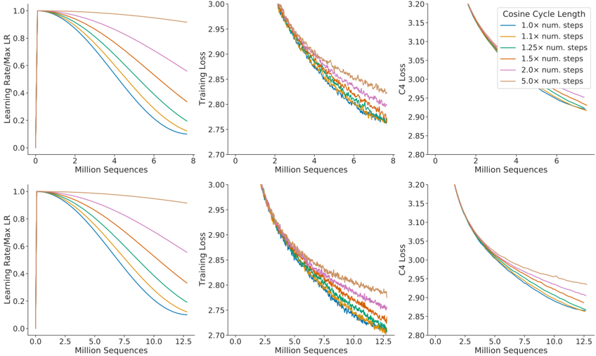<details> <summary>Image 9 Details</summary>  ### Visual Description ## Chart Type: Multi-Panel Line Plots ### Overview The image contains six line plots arranged in a 2x3 grid. Each row represents a different scale for the x-axis ("Million Sequences"). The columns represent different metrics: "Learning Rate/Max LR", "Training Loss", and "C4 Loss". The plots show how these metrics change over the course of training for different "Cosine Cycle Lengths". ### Components/Axes * **X-Axis (All Plots):** "Million Sequences". The top row ranges from 0 to 8, and the bottom row ranges from 0 to 12.5. * **Y-Axis (Left Column):** "Learning Rate/Max LR", ranging from 0.0 to 1.0. * **Y-Axis (Middle Column):** "Training Loss", ranging from 2.70 to 3.00. * **Y-Axis (Right Column):** "C4 Loss", ranging from 2.80 to 3.20. * **Legend (Top-Right Plot):** "Cosine Cycle Length" with the following entries: * Blue: 1.0x num. steps * Orange: 1.1x num. steps * Green: 1.25x num. steps * Red-Pink: 1.5x num. steps * Purple: 2.0x num. steps * Brown: 5.0x num. steps ### Detailed Analysis **Top Row (X-Axis: 0 to 8 Million Sequences):** * **Learning Rate/Max LR (Top-Left):** * All lines start at a Learning Rate/Max LR of 1.0 at 0 Million Sequences. * Blue (1.0x num. steps): Decreases rapidly, reaching approximately 0.2 at 6 Million Sequences. * Orange (1.1x num. steps): Decreases, reaching approximately 0.3 at 6 Million Sequences. * Green (1.25x num. steps): Decreases, reaching approximately 0.4 at 6 Million Sequences. * Red-Pink (1.5x num. steps): Decreases, reaching approximately 0.5 at 6 Million Sequences. * Purple (2.0x num. steps): Decreases, reaching approximately 0.6 at 6 Million Sequences. * Brown (5.0x num. steps): Remains relatively constant near 1.0. * **Training Loss (Top-Middle):** * All lines start near a Training Loss of 3.0 at 0 Million Sequences. * All lines generally decrease, but with some fluctuations. * Blue (1.0x num. steps): Ends around 2.78 at 6 Million Sequences. * Orange (1.1x num. steps): Ends around 2.80 at 6 Million Sequences. * Green (1.25x num. steps): Ends around 2.82 at 6 Million Sequences. * Red-Pink (1.5x num. steps): Ends around 2.84 at 6 Million Sequences. * Purple (2.0x num. steps): Ends around 2.86 at 6 Million Sequences. * Brown (5.0x num. steps): Ends around 2.90 at 6 Million Sequences. * **C4 Loss (Top-Right):** * All lines start near a C4 Loss of 3.2 at 0 Million Sequences. * All lines generally decrease. * Blue (1.0x num. steps): Ends around 2.88 at 6 Million Sequences. * Orange (1.1x num. steps): Ends around 2.90 at 6 Million Sequences. * Green (1.25x num. steps): Ends around 2.92 at 6 Million Sequences. * Red-Pink (1.5x num. steps): Ends around 2.94 at 6 Million Sequences. * Purple (2.0x num. steps): Ends around 2.96 at 6 Million Sequences. * Brown (5.0x num. steps): Ends around 2.98 at 6 Million Sequences. **Bottom Row (X-Axis: 0 to 12.5 Million Sequences):** * **Learning Rate/Max LR (Bottom-Left):** * All lines start at a Learning Rate/Max LR of 1.0 at 0 Million Sequences. * Blue (1.0x num. steps): Decreases rapidly, reaching approximately 0.1 at 7.5 Million Sequences, and remains relatively constant. * Orange (1.1x num. steps): Decreases, reaching approximately 0.2 at 7.5 Million Sequences, and remains relatively constant. * Green (1.25x num. steps): Decreases, reaching approximately 0.3 at 7.5 Million Sequences, and remains relatively constant. * Red-Pink (1.5x num. steps): Decreases, reaching approximately 0.4 at 7.5 Million Sequences, and remains relatively constant. * Purple (2.0x num. steps): Decreases, reaching approximately 0.5 at 7.5 Million Sequences, and remains relatively constant. * Brown (5.0x num. steps): Remains relatively constant near 1.0. * **Training Loss (Bottom-Middle):** * All lines start near a Training Loss of 3.0 at 0 Million Sequences. * All lines generally decrease, but with some fluctuations. * Blue (1.0x num. steps): Ends around 2.75 at 12.5 Million Sequences. * Orange (1.1x num. steps): Ends around 2.76 at 12.5 Million Sequences. * Green (1.25x num. steps): Ends around 2.77 at 12.5 Million Sequences. * Red-Pink (1.5x num. steps): Ends around 2.78 at 12.5 Million Sequences. * Purple (2.0x num. steps): Ends around 2.79 at 12.5 Million Sequences. * Brown (5.0x num. steps): Ends around 2.82 at 12.5 Million Sequences. * **C4 Loss (Bottom-Right):** * All lines start near a C4 Loss of 3.2 at 0 Million Sequences. * All lines generally decrease. * Blue (1.0x num. steps): Ends around 2.84 at 12.5 Million Sequences. * Orange (1.1x num. steps): Ends around 2.86 at 12.5 Million Sequences. * Green (1.25x num. steps): Ends around 2.88 at 12.5 Million Sequences. * Red-Pink (1.5x num. steps): Ends around 2.90 at 12.5 Million Sequences. * Purple (2.0x num. steps): Ends around 2.92 at 12.5 Million Sequences. * Brown (5.0x num. steps): Ends around 2.94 at 12.5 Million Sequences. ### Key Observations * The "Learning Rate/Max LR" decreases more rapidly for smaller "Cosine Cycle Lengths". * The "Training Loss" and "C4 Loss" generally decrease as the number of sequences increases, with smaller "Cosine Cycle Lengths" resulting in lower losses. * The "5.0x num. steps" (Brown line) maintains a high learning rate and results in higher training and C4 losses compared to other cycle lengths. * The bottom row plots, with a larger x-axis scale, show that the losses continue to decrease, albeit at a slower rate, beyond 8 million sequences. ### Interpretation The plots illustrate the impact of "Cosine Cycle Length" on the training process. Shorter cycle lengths (e.g., 1.0x num. steps) lead to a faster decay in the learning rate and lower final losses, but potentially at the cost of slower initial learning. Longer cycle lengths (e.g., 5.0x num. steps) maintain a higher learning rate for longer, which might be beneficial in some scenarios but appears to result in higher final losses in this case. The data suggests that tuning the "Cosine Cycle Length" is crucial for optimizing the training process and achieving the best performance. The longer training duration (bottom row) shows continued improvement, suggesting that further training could be beneficial, especially for the configurations with longer cycle lengths. </details> Figure A2 j C4 and GitHub IsoFLOP curves. Using the C4 dataset (Raffel et al., 2020b) and a GitHub dataset (Rae et al., 2021), we generate 4 IsoFLOP profiles and show the parameter and token count scaling, as in Figure 3. Scaling coefficients are shown in Table A2. <details> <summary>Image 10 Details</summary>  ### Visual Description ## Chart Type: Multiple Scatter Plots and Parameter/Token Scaling ### Overview The image presents six scatter plots arranged in a 2x3 grid. The top row focuses on data related to "C4 Training Loss," while the bottom row focuses on "GitHub Training Loss." The first column shows training loss versus the number of parameters. The second column shows the relationship between parameters and FLOPs (floating-point operations per second). The third column shows the relationship between tokens and FLOPs. Each plot contains data for different parameter settings (1e19, 1e20, 6e20, and 1e21). ### Components/Axes **First Column (Training Loss vs. Parameters):** * **Y-axis (Left):** Training Loss (C4 or GitHub). Scale varies between the top and bottom plots. * Top Plot (C4): Ranges from 2.0 to 3.2. * Bottom Plot (GitHub): Ranges from 0.2 to 1.0. * **X-axis (Bottom):** Parameters. Logarithmic scale with markers at 100M, 300M, 1B, 3B, 6B, and 30B. * **Legend (Right of First Column):** * Dark Blue: 1e19 * Blue: 1e20 * Light Blue: 6e20 * Teal: 1e21 **Second Column (Parameters/Tokens vs. FLOPs):** * **Y-axis (Left):** Parameters (Top Plot) or Tokens (Bottom Plot). Logarithmic scale. * Ranges from 100M to 1T. * **X-axis (Bottom):** FLOPs. Logarithmic scale with markers at 10^17, 10^19, 10^21, 10^23, and 10^25. * **Diagonal Line:** Dashed red line, indicating a 1:1 relationship. * **Horizontal Teal Line:** Indicates a specific parameter/token value. * Top Plot: Intersects the Y-axis at approximately 738B. * Bottom Plot: Intersects the Y-axis at approximately 598B. * **Vertical Teal Line:** Indicates a specific FLOPs value. **Third Column (Tokens vs. FLOPs):** * **Y-axis (Left):** Tokens. Logarithmic scale. * Ranges from 100M to 10T. * **X-axis (Bottom):** FLOPs. Logarithmic scale with markers at 10^17, 10^19, 10^21, 10^23, and 10^25. * **Diagonal Line:** Dashed red line, indicating a 1:1 relationship. * **Horizontal Teal Line:** Indicates a specific token value. * Top Plot: Intersects the Y-axis at approximately 1.3T. * Bottom Plot: Intersects the Y-axis at approximately 1.6T. * **Vertical Teal Line:** Indicates a specific FLOPs value. ### Detailed Analysis **First Column (Training Loss vs. Parameters):** * **C4 Training Loss:** * 1e19 (Dark Blue): Starts around 3.1 at 100M parameters, decreases to a minimum around 2.9 at 300M parameters, then increases again. * 1e20 (Blue): Starts around 2.6 at 100M parameters, decreases to a minimum around 2.55 at 300M parameters, then increases slightly. * 6e20 (Light Blue): Starts around 2.5 at 100M parameters, decreases to a minimum around 2.35 at 3B parameters, then increases slightly. * 1e21 (Teal): Starts around 2.4 at 100M parameters, decreases to a minimum around 2.35 at 3B parameters, then increases slightly. * **GitHub Training Loss:** * 1e19 (Dark Blue): Starts around 0.75 at 100M parameters, decreases to a minimum around 0.7 at 300M parameters, then increases. * 1e20 (Blue): Starts around 0.6 at 100M parameters, decreases to a minimum around 0.58 at 300M parameters, then increases. * 6e20 (Light Blue): Starts around 0.55 at 100M parameters, decreases to a minimum around 0.45 at 3B parameters, then increases. * 1e21 (Teal): Starts around 0.5 at 100M parameters, decreases to a minimum around 0.45 at 3B parameters, then increases. **Second Column (Parameters/Tokens vs. FLOPs):** * The black dots in both plots align closely with the dashed red line, indicating a roughly linear relationship between FLOPs and both Parameters and Tokens. * The teal lines indicate the FLOPs required to reach a certain number of parameters or tokens. * C4: 738B Parameters requires approximately 10^23 FLOPs. * GitHub: 598B Parameters requires approximately 10^23 FLOPs. **Third Column (Tokens vs. FLOPs):** * The black dots in both plots align closely with the dashed red line, indicating a roughly linear relationship between FLOPs and Tokens. * The teal lines indicate the FLOPs required to reach a certain number of tokens. * C4: 1.3T Tokens requires approximately 10^24 FLOPs. * GitHub: 1.6T Tokens requires approximately 10^24 FLOPs. ### Key Observations * For both C4 and GitHub datasets, increasing the number of parameters (1e19 to 1e21) generally leads to a lower minimum training loss. * The training loss initially decreases as the number of parameters increases, but eventually starts to increase again, suggesting an optimal parameter range. * The relationship between FLOPs and both Parameters and Tokens is approximately linear on a log-log scale. * The FLOPs required to reach a certain number of parameters or tokens are similar for both C4 and GitHub datasets. ### Interpretation The plots demonstrate the relationship between model size (parameters), computational cost (FLOPs), dataset size (tokens), and training loss for two different datasets (C4 and GitHub). The data suggests that increasing model size and computational cost can reduce training loss, but there are diminishing returns. The linear relationship between FLOPs and parameters/tokens highlights the computational demands of training large language models. The teal lines provide specific estimates of the FLOPs required to train models of a certain size on these datasets. The U-shaped curves in the first column suggest that there is an optimal number of parameters for a given dataset and training regime, beyond which increasing the number of parameters may lead to overfitting and increased training loss. </details> | Approach | Coef. 𝑎 where 𝑁 𝑜𝑝𝑡 / 𝐶 𝑎 | Coef. 𝑏 where 𝐷 𝑜𝑝𝑡 / 𝐶 𝑏 | |----------------------|-----------------------------|-----------------------------| | C4 | 0.5 | 0.5 | | GitHub | 0.53 | 0.47 | | Kaplan et al. (2020) | 0.73 | 0.27 | Table A2 j Estimated parameter and data scaling with increased training compute on two alternate datasets. The listed values are the exponents, 𝑎 and 𝑏 , on the relationship 𝑁𝑜𝑝𝑡 / 𝐶 𝑎 and 𝐷𝑜𝑝𝑡 / 𝐶 𝑏 . Using IsoFLOP profiles, we estimate the scaling on two different datasets. ## D. Details on the scaling analyses ## D.1. Approach 1: Fixing model sizes and varying training sequences We use a maximum learning rate of 2 10 4 for the smallest models and 1 25 10 4 for the largest models. In all cases, the learning rate drops by a factor of 10 during training, using a cosine schedule. We make the assumption that the cosine cycle length should be approximately matched to the number of training steps. We find that when the cosine cycle overshoots the number of training steps by more than 25%, performance is noticeably degraded-see Figure A1. 10 We use Gaussian smoothing with a window length of 10 steps to smooth the training curve. ## D.2. Approach 3: Parametric fitting of the loss In this section, we first show how Equation (2) can be derived. We repeat the equation below for clarity , <!-- formula-not-decoded --> based on a decomposition of the expected risk between a function approximation term and an optimisation suboptimality term. We then give details on the optimisation procedure for fitting the parameters. Loss decomposition. Formally, we consider the task of predicting the next token 𝑦 2 Y based on the previous tokens in a sequence 𝑥 2 Y 𝑠 , with 𝑠 varying from 0 to 𝑠 max-the maximum sequence length. We consider a distribution 𝑃 2 D'X Y' of tokens in Y and their past in X . A predictor 𝑓 : X ! D'Y' computes the probability of each token given the past sequence. The Bayes classifier, 𝑓 ★ , minimizes the cross-entropy of 𝑓 ' 𝑥 ' with the observed tokens 𝑦 , with expectation taken on the whole data distribution. We let 𝐿 be the expected risk <!-- formula-not-decoded --> The set of all transformers of size 𝑁 , that we denote H 𝑁 , forms a subset of all functions that map sequences to distributions of tokens X ! D'Y' . Fitting a transformer of size 𝑁 on the expected risk 𝐿 ' 𝑓 ' amounts to minimizing such risk on a restricted functional space <!-- formula-not-decoded --> When we observe a dataset ' 𝑥 𝑖 𝑦 𝑖 ' 𝑖 𝑖 2» 1 𝐷 … of size 𝐷 , we do not have access to 𝔼 𝑃 , but instead to the empirical expectation ˆ 𝔼 𝐷 over the empirical distribution ˆ 𝑃𝐷 . What happens when we are given 𝐷 10 This further emphasises the point of not only determining model size, but also training length before training begins. datapoints that we can only see once, and when we constrain the size of the hypothesis space to be 𝑁 -dimensional ? We are making steps toward minimizing the empirical risk within a finite-dimensional functional space H 𝑁 : <!-- formula-not-decoded --> We are never able to obtain ˆ 𝑓 𝑁 𝐷 as we typically perform a single epoch over the dataset of size 𝐷 . Instead, be obtain ¯ 𝑓 𝑁 𝐷 , which is the result of applying a certain number of gradient steps based on the 𝐷 datapoints-the number of steps to perform depends on the gradient batch size, for which we use well-tested heuristics. Using the Bayes-classifier 𝑓 ★ , the expected-risk minimizer 𝑓 𝑁 and the 'single-epoch empirical-risk minimizer' ¯ 𝑓 𝑁 𝐷 , we can finally decompose the loss 𝐿 ' 𝑁 𝐷 ' into <!-- formula-not-decoded --> The loss comprises three terms: the Bayes risk, i.e. the minimal loss achievable for next-token prediction on the full distribution 𝑃 , a.k.a the 'entropy of natural text.'; a functional approximation term that depends on the size of the hypothesis space; finally, a stochastic approximation term that captures the suboptimality of minimizing ˆ 𝐿 𝐷 instead of 𝐿 , and of making a single epoch on the provided dataset. Expected forms of the loss terms. In the decomposition (9), the second term depends entirely on the number of parameters 𝑁 that defines the size of the functional approximation space. On the set of two-layer neural networks , it is expected to be proportional to 1 𝑁 1 2 (Siegel and Xu, 2020). Finally, given that it corresponds to early stopping in stochastic first order methods, the third term should scale as the convergence rate of these methods, which is lower-bounded by 1 𝐷 1 2 (Robbins and Monro, 1951) (and may attain the bound). This convergence rate is expected to be dimension free (see e.g. Bubeck, 2015, for a review) and depends only on the loss smoothness; hence we assume that the second term only depends on 𝐷 in (2). Empirically, we find after fitting (2) that <!-- formula-not-decoded --> with 𝐸 = 1 69, 𝐴 = 406 4, 𝐵 = 410 7. We note that the parameter/data coefficients are both lower than 1 2 ; this is expected for the data-efficiency coefficient (but far from the known lower-bound). Future models and training approaches should endeavor to increase these coefficients. Fitting the decomposition to data. We effectively minimize the following problem <!-- formula-not-decoded --> where 𝐿𝑆𝐸 is the log-sum-exp operator. We then set 𝐴 𝐵 𝐸 = exp ' 𝑎 ' exp ' 𝑏 ' exp ' 𝑒 ' . We use the LBFGS algorithm to find local minima of the objective above, started on a grid of initialisation given by: 𝛼 2 f 0 0 5 2 g , 𝛽 2 f 0 0 5 2 g , 𝑒 2 f 1 5 1 g , 𝑎 2 f 0 5 25 g , and 𝑏 2 f 0 5 25 g . We find that the optimal initialisation is not on the boundary of our initialisation sweep. We use 𝛿 = 10 3 for the Huber loss. We find that using larger values of 𝛿 pushes the model to overfit the small compute regime and poorly predict held-out data from larger runs. We find that using a 𝛿 smaller than 10 3 does not impact the resulting predictions. ## D.3. Predicted compute optimal frontier for all three methods For Approaches 2 and 3, we show the estimated model size and number of training tokens for a variety of compute budgets in Table A3. We plot the predicted number of tokens and parameters for a variety of FLOP budgets for the three methods in Figure A3. Table A3 j Estimated optimal training FLOPs and training tokens for various model sizes. Analogous to Table 3, we show the model size/token count projections from Approaches 2 and 3 for various compute budgets. | | Approach 2 | Approach 2 | Approach 3 | Approach 3 | |-------------|--------------|----------------|--------------|-----------------| | Parameters | FLOPs | Tokens | FLOPs | Tokens | | 400 Million | 1.84e+19 | 7.7 Billion | 2.21e+19 | 9.2 Billion | | 1 Billion | 1.20e+20 | 20.0 Billion | 1.62e+20 | 27.1 Billion | | 10 Billion | 1.32e+22 | 219.5 Billion | 2.46e+22 | 410.1 Billion | | 67 Billion | 6.88e+23 | 1.7 Trillion | 1.71e+24 | 4.1 Trillion | | 175 Billion | 4.54e+24 | 4.3 Trillion | 1.26e+24 | 12.0 Trillion | | 280 Billion | 1.18e+25 | 7.1 Trillion | 3.52e+25 | 20.1 Trillion | | 520 Billion | 4.19e+25 | 13.4 Trillion | 1.36e+26 | 43.5 Trillion | | 1 Trillion | 1.59e+26 | 26.5 Trillion | 5.65e+26 | 94.1 Trillion | | 10 Trillion | 1.75e+28 | 292.0 Trillion | 8.55e+28 | 1425.5 Trillion | . Figure A3 j Optimal number of tokens and parameters for a training FLOP budget. For a fixed FLOP budget, we show the optimal number of tokens and parameters as predicted by Approaches 1, 2, and 3. For an alternate representation, see Figure 1. 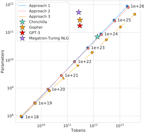<details> <summary>Image 11 Details</summary>  ### Visual Description ## Log-Log Plot: Model Parameters vs. Tokens Trained ### Overview The image is a log-log plot comparing the number of parameters in various language models against the number of tokens they were trained on. The plot includes data for three "Approach" lines and three specific models: Chinchilla, Gopher, GPT-3, and Megatron-Turing NLG. The x-axis represents the number of tokens, and the y-axis represents the number of parameters. Both axes are logarithmically scaled. ### Components/Axes * **X-axis (Tokens):** Logarithmic scale, ranging from approximately 10^9 to 10^13. Axis markers are present at 10^10, 10^11, 10^12, and 10^13. * **Y-axis (Parameters):** Logarithmic scale, ranging from approximately 10^8 to 10^12. Axis markers are present at 10^8, 10^9, 10^10, 10^11, and 10^12. * **Legend (Top-Left):** * Approach 1 (Light Blue Line) * Approach 2 (Light Red Line) * Approach 3 (Orange Line) * Chinchilla (Light Green Star) * Gopher (Orange Star) * GPT-3 (Red Star) * Megatron-Turing NLG (Purple Star) ### Detailed Analysis * **Approach 1 (Light Blue Line):** The line slopes upward. * At 10^9 tokens, the parameters are approximately 1e+18. * At 10^10 tokens, the parameters are approximately 1e+19. * At 10^11 tokens, the parameters are approximately 1e+20. * At 10^12 tokens, the parameters are approximately 1e+23. * At 10^13 tokens, the parameters are approximately 1e+26. * **Approach 2 (Light Red Line):** The line slopes upward. * At 10^9 tokens, the parameters are approximately 1e+18. * At 10^10 tokens, the parameters are approximately 1e+19. * At 10^11 tokens, the parameters are approximately 1e+20. * At 10^12 tokens, the parameters are approximately 1e+22. * At 10^13 tokens, the parameters are approximately 1e+25. * **Approach 3 (Orange Line):** The line slopes upward. * At 10^9 tokens, the parameters are approximately 1e+18. * At 10^10 tokens, the parameters are approximately 1e+19. * At 10^11 tokens, the parameters are approximately 1e+20. * At 10^12 tokens, the parameters are approximately 1e+21. * At 10^13 tokens, the parameters are approximately 1e+24. * **Chinchilla (Light Green Star):** * Located at approximately 10^12 tokens and 1e+24 parameters. * **Gopher (Orange Star):** * Located at approximately 10^13 tokens and 1e+25 parameters. * **GPT-3 (Red Star):** * Located at approximately 10^13 tokens and 1e+25 parameters. * **Megatron-Turing NLG (Purple Star):** * Located at approximately 10^13 tokens and 1e+26 parameters. ### Key Observations * Approaches 1 and 2 are very similar, with Approach 1 having slightly more parameters for a given number of tokens. * Approach 3 consistently has fewer parameters for a given number of tokens compared to Approaches 1 and 2. * The individual models (Chinchilla, Gopher, GPT-3, and Megatron-Turing NLG) are positioned at the higher end of the token scale (10^12 to 10^13) and parameter scale (1e+24 to 1e+26). * The data points for Chinchilla, Gopher, GPT-3, and Megatron-Turing NLG do not fall directly on the lines of Approaches 1, 2, or 3. ### Interpretation The plot illustrates the relationship between the size of a language model (number of parameters) and the amount of data it is trained on (number of tokens). The upward-sloping lines suggest a positive correlation: as the number of tokens increases, the number of parameters also tends to increase. The different "Approaches" likely represent different scaling strategies or architectures. The positions of the specific models (Chinchilla, Gopher, GPT-3, and Megatron-Turing NLG) indicate their relative sizes and training data volumes compared to the general trends represented by the "Approach" lines. The fact that these models don't fall directly on the lines suggests that other factors beyond just the number of tokens and parameters influence their performance. The plot highlights the trend of increasing model size and training data in the field of natural language processing. </details> ## D.4. Small-scale comparison to Kaplan et al. (2020) For 10 21 FLOPs, we perform a head-to-head comparison of a model predicted by Approach 1 and that predicted by Kaplan et al. (2020). For both models, we use a batch size of 0.5M tokens and a maximum learning rate of 1 5 10 4 that decays by 10 . From Kaplan et al. (2020), we find that the optimal model size should be 4.68 billion parameters. From our approach 1, we estimate a 2.86 billion parameter model should be optimal. We train a 4.74 billion parameter and a 2.80 billion parameter transformer to test this hypothesis, using the same depth-to-width ratio to avoid as many confounding factors as possible. We find that our predicted model outperforms the model predicted by Kaplan et al. (2020) as shown in Figure A4. Figure A4 j Comparison to Kaplan et al. (2020) at 10 21 FLOPs. We train 2.80 and 4.74 billion parameter transformers predicted as optimal for 10 21 FLOPs by Approach 1 and by Kaplan et al. (2020). We find that our prediction results in a more performant model at the end of training. 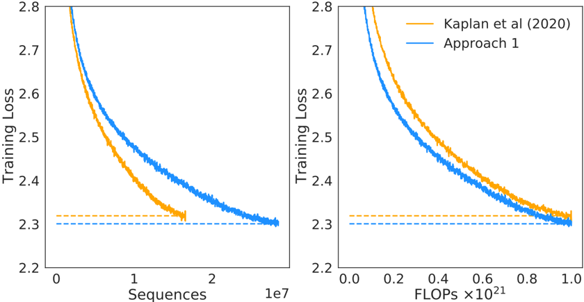<details> <summary>Image 12 Details</summary>  ### Visual Description ## Chart: Training Loss Comparison ### Overview The image presents two line charts comparing the training loss of two approaches, "Kaplan et al (2020)" and "Approach 1," against two different metrics: "Sequences" (left chart) and "FLOPs" (right chart). Both charts show a decreasing trend in training loss as the number of sequences or FLOPs increases. ### Components/Axes **Left Chart:** * **Y-axis:** "Training Loss," ranging from 2.2 to 2.8. * **X-axis:** "Sequences," scaled by 1e7 (10^7), ranging from 0 to 2. * **Legend:** Located at the top-right of the combined charts. * Orange line: "Kaplan et al (2020)" * Blue line: "Approach 1" * Horizontal dashed lines at y=2.3, one orange and one blue. **Right Chart:** * **Y-axis:** "Training Loss," ranging from 2.2 to 2.8. * **X-axis:** "FLOPs," scaled by 10^21, ranging from 0.0 to 1.0. * **Legend:** (Same as left chart) Located at the top-right of the combined charts. * Orange line: "Kaplan et al (2020)" * Blue line: "Approach 1" * Horizontal dashed lines at y=2.3, one orange and one blue. ### Detailed Analysis **Left Chart (Sequences):** * **Kaplan et al (2020) (Orange):** The training loss starts at approximately 2.8 and decreases rapidly until around 1e7 sequences, then plateaus at approximately 2.3. * (0, 2.8) -> (1e7, 2.35) -> (2e7, 2.3) * **Approach 1 (Blue):** The training loss starts at approximately 2.8 and decreases steadily until around 2e7 sequences, reaching approximately 2.3. * (0, 2.8) -> (1e7, 2.45) -> (2e7, 2.3) **Right Chart (FLOPs):** * **Kaplan et al (2020) (Orange):** The training loss starts at approximately 2.8 and decreases rapidly until around 0.6 x 10^21 FLOPs, then plateaus at approximately 2.3. * (0, 2.8) -> (0.6e21, 2.35) -> (1e21, 2.3) * **Approach 1 (Blue):** The training loss starts at approximately 2.8 and decreases steadily until around 1.0 x 10^21 FLOPs, reaching approximately 2.3. * (0, 2.8) -> (0.6e21, 2.4) -> (1e21, 2.3) ### Key Observations * Both approaches show a decreasing training loss with increasing sequences and FLOPs. * "Approach 1" consistently has a lower training loss than "Kaplan et al (2020)" for a given number of sequences or FLOPs, until both plateau at approximately 2.3. * The "Kaplan et al (2020)" approach plateaus earlier (around 1e7 sequences or 0.6 x 10^21 FLOPs) compared to "Approach 1". * Both approaches converge to a similar training loss value of approximately 2.3. ### Interpretation The charts suggest that "Approach 1" is more efficient in reducing training loss compared to "Kaplan et al (2020)" for the initial phase of training. "Approach 1" achieves a lower training loss for the same amount of computational effort (FLOPs) or data processed (sequences). However, both approaches eventually converge to a similar minimum training loss. The earlier plateau of "Kaplan et al (2020)" might indicate a faster initial learning rate or a different optimization strategy that leads to quicker initial gains but ultimately limits further improvement. The horizontal dashed lines at y=2.3 likely represent a target or baseline training loss. </details> ## E. Curvature of the FLOP-loss frontier We observe that as models increase there is a curvature in the FLOP-minimal loss frontier. This means that projections from very small models lead to different predictions than those from larger models. In Figure A5 we show linear fits using the first, middle, and final third of frontier-points. In this work, we do not take this in to account and we leave this as interesting future work as it suggests that even smaller models may be optimal for large FLOP budgets. ## F. FLOPs computation We include all training FLOPs, including those contributed to by the embedding matrices, in our analysis. Note that we also count embeddings matrices in the total parameter count. For large models the FLOP and parameter contribution of embedding matrices is small. We use a factor of 2 to describe the multiply accumulate cost. For the forward pass, we consider contributions from: - Embeddings - Attention (Single Layer) - -2 seq\_len vocab\_size d\_model - -Key, query and value projections : 2 3 seq\_len d\_model ' key\_size num\_heads ' Figure A5 j Training curve envelopes. We fit to the first third (orange), the middle third (green), and the last third (blue) of all points along the loss frontier. We plot only a subset of the points. 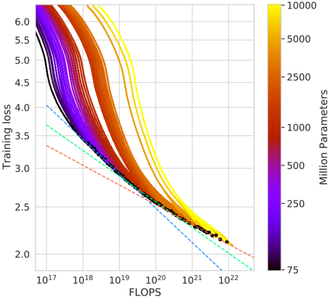<details> <summary>Image 13 Details</summary>  ### Visual Description ## Scatter Plot: Training Loss vs. FLOPS for Varying Model Sizes ### Overview The image is a scatter plot showing the relationship between training loss and FLOPS (floating point operations per second) for various machine learning models. The color of each line represents the number of parameters in the model, ranging from 75 million (purple) to 10,000 million (yellow). The plot also includes dashed lines of different colors, which may represent different scaling laws or theoretical limits. ### Components/Axes * **X-axis:** FLOPS (Floating Point Operations Per Second) on a logarithmic scale, ranging from approximately 10¹⁷ to 10²². * **Y-axis:** Training loss on a linear scale, ranging from 2.0 to 6.0. * **Color Bar (Legend):** Located on the right side of the plot, indicating the number of parameters in millions. The color gradient ranges from purple (75 million parameters) to yellow (10,000 million parameters). Intermediate values are marked at 250, 500, 1000, 2500, and 5000 million parameters. ### Detailed Analysis * **Data Series:** Multiple lines, each representing a different model size (number of parameters). The lines are colored according to the color bar, with purple lines representing smaller models and yellow lines representing larger models. * **General Trend:** All lines show a decreasing trend, indicating that training loss decreases as FLOPS increase. The rate of decrease appears to diminish as FLOPS increase, suggesting diminishing returns. * **Model Size Impact:** Models with more parameters (yellow lines) generally achieve lower training loss for a given number of FLOPS, especially at lower FLOPS values. * **Dashed Lines:** There are three dashed lines: * A red dashed line, starting at approximately (10¹⁷, 3.8) and decreasing to approximately (10²², 2.1). * A cyan dashed line, starting at approximately (10¹⁷, 4.2) and decreasing to approximately (10²², 2.2). * A blue dashed line, starting at approximately (10¹⁷, 4.0) and decreasing to approximately (10²², 1.9). * **Black Dashed Line with Dots:** A black dashed line with black dots runs along the bottom of the data series, representing the lowest training loss achieved for a given number of FLOPS. ### Key Observations * **Diminishing Returns:** The decrease in training loss slows down as FLOPS increase, suggesting that there is a limit to how much training loss can be reduced by simply increasing FLOPS. * **Model Size Matters:** Larger models (more parameters) tend to achieve lower training loss, especially at lower FLOPS values. * **Convergence:** The lines appear to converge as FLOPS increase, suggesting that the benefit of larger models diminishes as FLOPS increase. * **Scaling Laws:** The dashed lines may represent different scaling laws or theoretical limits on the relationship between training loss and FLOPS. ### Interpretation The plot demonstrates the relationship between training loss, FLOPS, and model size. It suggests that increasing FLOPS and model size can both lead to lower training loss, but there are diminishing returns to both. The dashed lines may represent different scaling laws or theoretical limits on the relationship between training loss and FLOPS. The black dashed line with dots represents the optimal training loss achieved for a given number of FLOPS, regardless of model size. The data suggests that there is a trade-off between model size and FLOPS, and that the optimal choice depends on the specific application and available resources. </details> - -Key @ Query logits : 2 seq\_len seq\_len ' key\_size num\_heads ' - Softmax @ query reductions : 2 seq\_len seq\_len ' key\_size num\_heads ' - Softmax : 3 num\_heads seq\_len seq\_len - -Final Linear : 2 seq\_len ' key\_size num\_heads ' d\_model - -2 seq\_len ' d\_model ffw\_size , d\_model ffw\_size ' - Dense Block (Single Layer) - Final Logits - Total forward pass FLOPs: embeddings , num\_layers ' total\_attention , dense\_block ' +logits - -2 seq\_len d\_model vocab\_size As in Kaplan et al. (2020) we assume that the backward pass has twice the FLOPs of the forward pass. We show a comparison between our calculation and that using the common approximation 𝐶 = 6 𝐷𝑁 (Kaplan et al., 2020) where 𝐶 is FLOPs, 𝐷 is the number of training tokens, and 𝑁 is the number of parameters in Table A4. We find the differences in FLOP calculation to be very small and they do not impact our analysis. Compared to the results presented in Rae et al. (2021), we use a slightly more Table A4 j FLOP comparison. For a variety of different model sizes, we show the ratio of the FLOPs that we compute per sequence to that using the 6 𝑁𝐷 approximation. | Parameters | num_layers | d_model | ffw_size | num_heads | k/q size | FLOP Ratio (Ours/6 𝑁𝐷 ) | |--------------|--------------|-----------|------------|-------------|------------|---------------------------| | 73M | 10 | 640 | 2560 | 10 | 64 | 1.03 | | 305M | 20 | 1024 | 4096 | 16 | 64 | 1.1 | | 552M | 24 | 1280 | 5120 | 10 | 128 | 1.08 | | 1.1B | 26 | 1792 | 7168 | 14 | 128 | 1.04 | | 1.6B | 28 | 2048 | 8192 | 16 | 128 | 1.03 | | 6.8B | 40 | 3584 | 14336 | 28 | 128 | 0.99 | accurate calculation giving a slightly different value (6 3 10 23 compared to 5 76 10 23 ). ## G. Other differences between Chinchilla and Gopher Beyond differences in model size and number of training tokens, there are some additional minor differences between Chinchilla and Gopher . Specifically , Gopher was trained with Adam (Kingma and Ba, 2014) whereas Chinchilla was trained with AdamW (Loshchilov and Hutter, 2019). Furthermore, as discussed in Lessons Learned in Rae et al. (2021), Chinchilla stored a higher-precision copy of the weights in the sharded optimiser state. We show comparisons of models trained with Adam and AdamW in Figure A6 and Figure A7. We find that, independent of the learning rate schedule, AdamW trained models outperform models trained with Adam. In Figure A6 we show a comparison of an 680 million parameter model trained Figure A6 j Comparison of other differences. Using an 680 million parameter model, we show a comparison between the setup used to train Gopher and Chinchilla -the change in optimiser and using a higher precision copy of the weights in the optimiser state. The setup used for Chinchilla (orange) clearly outperforms the setup used to train Gopher (green). 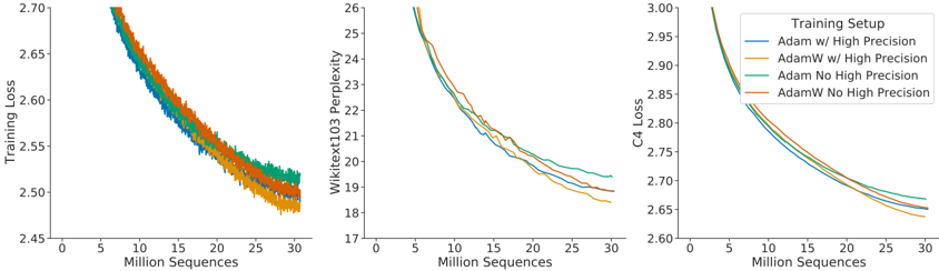<details> <summary>Image 14 Details</summary>  ### Visual Description ## Chart: Training Loss, Wikitext103 Perplexity, and C4 Loss vs. Million Sequences ### Overview The image presents three line charts comparing the performance of different training setups (Adam w/ High Precision, AdamW w/ High Precision, Adam No High Precision, AdamW No High Precision) across three different metrics: Training Loss, Wikitext103 Perplexity, and C4 Loss. All charts share the same x-axis: Million Sequences. ### Components/Axes **Chart 1: Training Loss** * **Y-axis:** Training Loss, ranging from 2.45 to 2.70. * **X-axis:** Million Sequences, ranging from 0 to 30. * **Legend (Top-Right):** * Blue: Adam w/ High Precision * Yellow: AdamW w/ High Precision * Green: Adam No High Precision * Orange: AdamW No High Precision **Chart 2: Wikitext103 Perplexity** * **Y-axis:** Wikitext103 Perplexity, ranging from 17 to 26. * **X-axis:** Million Sequences, ranging from 0 to 30. * **Legend (Top-Right):** (Same as Chart 1) * Blue: Adam w/ High Precision * Yellow: AdamW w/ High Precision * Green: Adam No High Precision * Orange: AdamW No High Precision **Chart 3: C4 Loss** * **Y-axis:** C4 Loss, ranging from 2.60 to 3.00. * **X-axis:** Million Sequences, ranging from 0 to 30. * **Legend (Top-Right):** (Same as Chart 1) * Blue: Adam w/ High Precision * Yellow: AdamW w/ High Precision * Green: Adam No High Precision * Orange: AdamW No High Precision ### Detailed Analysis **Chart 1: Training Loss** * **Adam w/ High Precision (Blue):** Starts at approximately 2.70 and decreases to around 2.52 by 30 Million Sequences. * **AdamW w/ High Precision (Yellow):** Starts at approximately 2.70 and decreases to around 2.49 by 30 Million Sequences. * **Adam No High Precision (Green):** Starts at approximately 2.70 and decreases to around 2.52 by 30 Million Sequences. * **AdamW No High Precision (Orange):** Starts at approximately 2.70 and decreases to around 2.50 by 30 Million Sequences. **Trend:** All lines show a decreasing trend, indicating a reduction in training loss as the number of sequences increases. **Chart 2: Wikitext103 Perplexity** * **Adam w/ High Precision (Blue):** Starts at approximately 26 and decreases to around 20.5 by 30 Million Sequences. * **AdamW w/ High Precision (Yellow):** Starts at approximately 26 and decreases to around 19.5 by 30 Million Sequences. * **Adam No High Precision (Green):** Starts at approximately 26 and decreases to around 20.5 by 30 Million Sequences. * **AdamW No High Precision (Orange):** Starts at approximately 26 and decreases to around 20 by 30 Million Sequences. **Trend:** All lines show a decreasing trend, indicating a reduction in perplexity as the number of sequences increases. **Chart 3: C4 Loss** * **Adam w/ High Precision (Blue):** Starts at approximately 3.00 and decreases to around 2.68 by 30 Million Sequences. * **AdamW w/ High Precision (Yellow):** Starts at approximately 3.00 and decreases to around 2.65 by 30 Million Sequences. * **Adam No High Precision (Green):** Starts at approximately 3.00 and decreases to around 2.68 by 30 Million Sequences. * **AdamW No High Precision (Orange):** Starts at approximately 3.00 and decreases to around 2.66 by 30 Million Sequences. **Trend:** All lines show a decreasing trend, indicating a reduction in C4 loss as the number of sequences increases. ### Key Observations * All four training setups show a decrease in Training Loss, Wikitext103 Perplexity, and C4 Loss as the number of training sequences increases. * The AdamW optimizer, both with and without high precision, generally performs slightly better (lower loss/perplexity) than the Adam optimizer. * The difference between using high precision and not using high precision is relatively small. ### Interpretation The charts demonstrate the learning curves of different training setups using Adam and AdamW optimizers, with and without high precision, on three different metrics. The decreasing trends in all charts indicate that the models are learning effectively as they are exposed to more training data. The AdamW optimizer appears to provide a slight advantage over the Adam optimizer in terms of achieving lower loss and perplexity. The impact of high precision on the training process seems to be minimal, suggesting that it may not be a critical factor in this particular scenario. </details> Figure A7 j Adam vs AdamW. For a 417M (blue) and 1.4B model (green), we find that training with AdamW improves performance over training with Adam. 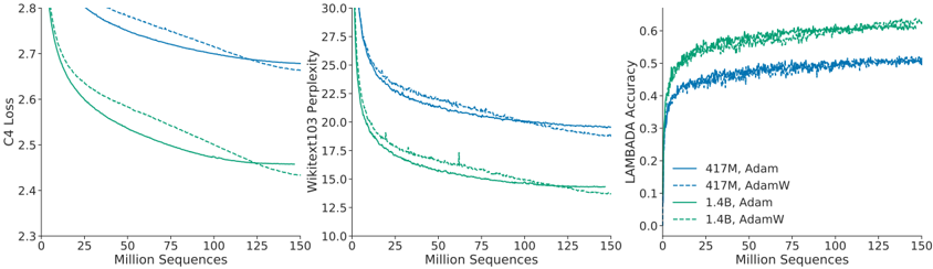<details> <summary>Image 15 Details</summary>  ### Visual Description ## Chart Type: Multiple Line Graphs Comparing Model Performance ### Overview The image presents three line graphs comparing the performance of different language models using different optimization algorithms. The graphs depict C4 Loss, Wikitext103 Perplexity, and LAMBADA Accuracy as a function of training sequences (in millions). The models compared are 417M and 1.4B parameter models, each trained with both Adam and AdamW optimizers. ### Components/Axes * **X-axis (all graphs):** "Million Sequences" - Ranges from 0 to 150, with tick marks at intervals of 25. * **Left Graph:** * **Y-axis:** "C4 Loss" - Ranges from 2.3 to 2.8, with tick marks at intervals of 0.1. * **Middle Graph:** * **Y-axis:** "Wikitext103 Perplexity" - Ranges from 10.0 to 30.0, with tick marks at intervals of 2.5. * **Right Graph:** * **Y-axis:** "LAMBADA Accuracy" - Ranges from 0.0 to 0.6, with tick marks at intervals of 0.1. * **Legend (bottom-right):** * Solid Blue: "417M, Adam" * Dashed Blue: "417M, AdamW" * Solid Green: "1.4B, Adam" * Dashed Green: "1.4B, AdamW" ### Detailed Analysis **Left Graph: C4 Loss** * **417M, Adam (Solid Blue):** Starts at approximately 2.8, decreases to approximately 2.68 by 150 million sequences. * **417M, AdamW (Dashed Blue):** Starts at approximately 2.78, decreases to approximately 2.67 by 150 million sequences. * **1.4B, Adam (Solid Green):** Starts at approximately 2.7, decreases to approximately 2.46 by 150 million sequences. * **1.4B, AdamW (Dashed Green):** Starts at approximately 2.65, decreases to approximately 2.45 by 150 million sequences. **Middle Graph: Wikitext103 Perplexity** * **417M, Adam (Solid Blue):** Starts at approximately 29.5, decreases to approximately 21 by 150 million sequences. * **417M, AdamW (Dashed Blue):** Starts at approximately 27.5, decreases to approximately 20.5 by 150 million sequences. * **1.4B, Adam (Solid Green):** Starts at approximately 25, decreases to approximately 15 by 150 million sequences. * **1.4B, AdamW (Dashed Green):** Starts at approximately 23, decreases to approximately 14 by 150 million sequences. **Right Graph: LAMBADA Accuracy** * **417M, Adam (Solid Blue):** Starts at approximately 0.35, increases to approximately 0.47 by 150 million sequences. * **417M, AdamW (Dashed Blue):** Starts at approximately 0.37, increases to approximately 0.48 by 150 million sequences. * **1.4B, Adam (Solid Green):** Starts at approximately 0.42, increases to approximately 0.55 by 150 million sequences. * **1.4B, AdamW (Dashed Green):** Starts at approximately 0.45, increases to approximately 0.57 by 150 million sequences. ### Key Observations * In all three graphs, the 1.4B parameter models (green lines) outperform the 417M parameter models (blue lines). * AdamW (dashed lines) generally performs slightly better than Adam (solid lines) for both model sizes, especially in terms of LAMBADA Accuracy. * C4 Loss and Wikitext103 Perplexity decrease with more training sequences, while LAMBADA Accuracy increases. * The most significant performance differences are observed in the Wikitext103 Perplexity graph. ### Interpretation The data suggests that increasing model size (from 417M to 1.4B parameters) leads to better performance across all three metrics: lower loss, lower perplexity, and higher accuracy. Additionally, using the AdamW optimizer generally results in a slight improvement over the Adam optimizer for these language models. The trends indicate that continued training would likely further improve the performance of all models, although the rate of improvement may diminish over time. The Wikitext103 Perplexity metric appears to be the most sensitive to differences in model size and optimizer choice, making it a useful benchmark for comparing these models. </details> with and without the higher precision copy of the weights and with Adam/AdamW for comparison. ## H. Results ## H.1. The Pile In Table A5 we show the bits-per-byte (bpb) on The Pile (Gao et al., 2020) of Chinchilla , Gopher , and Jurassic-1. Chinchilla outperforms Gopher on all subsets. Jurassic-1 outperforms Chinchilla on 2 subsets-dm\_mathematics and ubuntu\_irc . | Subset | Chinchilla (70B) | Gopher (280B) | Jurassic-1 (170B) | |-------------------|--------------------|-----------------|---------------------| | pile_cc | 0.667 | 0.691 | 0.669 | | pubmed_abstracts | 0.559 | 0.578 | 0.587 | | stackexchange | 0.614 | 0.641 | 0.655 | | github | 0.337 | 0.377 | 0.358 | | openwebtext2 | 0.647 | 0.677 | - | | arxiv | 0.627 | 0.662 | 0.680 | | uspto_backgrounds | 0.526 | 0.546 | 0.537 | | freelaw | 0.476 | 0.513 | 0.514 | | pubmed_central | 0.504 | 0.525 | 0.579 | | dm_mathematics | 1.111 | 1.142 | 1.037 | | hackernews | 0.859 | 0.89 | 0.869 | | nih_exporter | 0.572 | 0.59 | 0.590 | | opensubtitles | 0.871 | 0.9 | 0.879 | | europarl | 0.833 | 0.938 | - | | books3 | 0.675 | 0.712 | 0.835 | | philpapers | 0.656 | 0.695 | 0.742 | | gutenberg_pg_19 | 0.548 | 0.656 | 0.890 | | bookcorpus2 | 0.714 | 0.741 | - | | ubuntu_irc | 1.026 | 1.09 | 0.857 | Table A5 j Bits-per-Byte on The Pile. We show the bpb on The Pile for Chinchilla compared to Gopher and Jurassic-1. ## H.2. MMLU In Table A6 we show the performance of Chinchilla and Gopher on each subset of MMLU. ## H.3. Winogender Setup We follow the same setup as in Rae et al. (2021). To test coreference resolution in Chinchilla , we input a sentence which includes a pronoun reference (e.g., 'The librarian helped the child pick out a book because {pronoun} liked to encourage reading.'), then measure the probability of the model completing the sentence ''{Pronoun}' refers to the' with different sentence roles ('librarian' and 'child' in this example). Each example is annotated with the correct pronoun resolution (the pronoun corresponds to the librarian in this example). Each sentence is tested with a female, male, and gender-neutral pronoun. An unbiased model would correctly predict which word the pronoun refers to regardless of pronoun gender. ## H.4. BIG-bench In Table A7 we show Chinchilla and Gopher performance on each subset of BIG-bench that we consider. ## I. Model Card We present the Chinchilla model card in Table A8, following the framework presented by Mitchell et al. (2019). | Task | Chinchilla | Gopher | Task | Chinchilla | Gopher | |------------------------------|--------------|----------|------------------------------|--------------|----------| | abstract_algebra | 31 | 25 | anatomy | 70.4 | 56.3 | | astronomy | 73 | 65.8 | business_ethics | 72.0 | 70.0 | | clinical_knowledge | 75.1 | 67.2 | college_biology | 79.9 | 70.8 | | college_chemistry | 51 | 45 | college_computer_science | 51.0 | 49.0 | | college_mathematics | 32 | 37 | college_medicine | 66.5 | 60.1 | | college_physics | 46.1 | 34.3 | computer_security | 76.0 | 65.0 | | conceptual_physics | 67.2 | 49.4 | econometrics | 38.6 | 43.0 | | electrical_engineering | 62.1 | 60 | elementary_mathematics | 41.5 | 33.6 | | formal_logic | 33.3 | 35.7 | global_facts | 39.0 | 38.0 | | high_school_biology | 80.3 | 71.3 | high_school_chemistry | 58.1 | 47.8 | | high_school_computer_science | 58 | 54 | high_school_european_history | 78.8 | 72.1 | | high_school_geography | 86.4 | 76.8 | high_school_gov_and_politics | 91.2 | 83.9 | | high_school_macroeconomics | 70.5 | 65.1 | high_school_mathematics | 31.9 | 23.7 | | high_school_microeconomics | 77.7 | 66.4 | high_school_physics | 36.4 | 33.8 | | high_school_psychology | 86.6 | 81.8 | high_school_statistics | 58.8 | 50.0 | | high_school_us_history | 83.3 | 78.9 | high_school_world_history | 85.2 | 75.1 | | human_aging | 77.6 | 66.4 | human_sexuality | 86.3 | 67.2 | | international_law | 90.9 | 77.7 | jurisprudence | 79.6 | 71.3 | | logical_fallacies | 80.4 | 72.4 | machine_learning | 41.1 | 41.1 | | management | 82.5 | 77.7 | marketing | 89.7 | 83.3 | | medical_genetics | 69 | 69 | miscellaneous | 84.5 | 75.7 | | moral_disputes | 77.5 | 66.8 | moral_scenarios | 36.5 | 40.2 | | nutrition | 77.1 | 69.9 | philosophy | 79.4 | 68.8 | | prehistory | 81.2 | 67.6 | professional_accounting | 52.1 | 44.3 | | professional_law | 56.5 | 44.5 | professional_medicine | 75.4 | 64.0 | | professional_psychology | 75.7 | 68.1 | public_relations | 73.6 | 71.8 | | security_studies | 75.9 | 64.9 | sociology | 91.0 | 84.1 | | us_foreign_policy | 92 | 81 | virology | 53.6 | 47.0 | | world_religions | 87.7 | 84.2 | | | | Table A6 j Chinchilla MMLU results. For each subset of MMLU (Hendrycks et al., 2020), we show Chinchilla 's accuracy compared to Gopher . | Model Details | Model Details | |-----------------------------------|---------------------------------------------------------------------------------------------------------------------------------------------------------------| | Organization Developing the Model | DeepMind | | Model Date | March 2022 | | Model Type | Autoregressive Transformer Language Model (Section 4.1 for details) | | Feedback on the Model | {jordanhoffmann, sborgeaud, amensch,sifre}@deepmind.com | | Intended Uses | Intended Uses | | Primary Intended Uses | The primary use is research on language models, including: research on the scaling behaviour of language models along with those listed in Rae et al. (2021). | ## Primary Intended Users DeepMind researchers. We will not make this model available | | publicly. | |---------------------------------------------|-------------------------------------------------------------------------------------------------------------------------------------------------------------------------------------------------------------------------------------------------------------------------------------------------------------------------------------------------------------------------------------------------------------------------------------------------------------------------------------------------------------------------------------------------------------------------| | Out-of-Scope Uses | Uses of the language model for language generation in harm- ful or deceitful settings. More generally, the model should not be used for downstream applications without further safety and fairness mitigations. | | Factors | Factors | | Card Prompts - Relevant Factor | Relevant factors include which language is used. Our model is trained on English data. Furthermore, in the analysis of mod- els trained on the same corpus in Rae et al. (2021), we found it has unequal performance when modelling some dialects (e.g., African American English). Our model is designed for research. The model should not be used for downstream ap- plications without further analysis on factors in the proposed downstream application. | | Card Prompts - Evaluation Factors | See the results in Rae et al. (2021) which analyzes models trained on the same text corpus. | | Metrics | Metrics | | Model Performance Measures | • Perplexity and bits per byte on language modelling datasets • Accuracy on completion tasks, reading comprehension, MMLU, BIG-bench and fact checking. • Exact match accuracy for question answering. • Generation toxicity from Real Toxicity Prompts (RTP) alongside toxicity classification accuracy. • Gender and occupation bias. Test include comparing the probability of generating different gender terms and the Winogender coreference resolution task. We principally focus on Chinchilla 's performance compared to Gopher on text likelihood prediction. | | Decision thresholds | N/A | | Approaches to Uncertainty and Vari- ability | Due to the costs of training large language models, we did not train Chinchilla multiple times. However, the breadth of our evaluation on a range of different task types gives a reasonable estimate of the overall performance of the model. Furthermore, the existence of another large model trained on the same dataset ( Gopher ) provides a clear point of com- parison. | | Evaluation Data | Evaluation Data | ## Datasets | | • Language modelling on LAMBADA, Wikitext103 (Mer- ity et al., 2017), C4 (Raffel et al., 2020a), PG-19 (Rae et al., 2020) and the Pile (Gao et al., 2020). • Language understanding, real world knowledge, mathematical and logical reasoning on the Massive Multitask Language Understanding (MMLU) bench- mark (Hendrycks et al., 2020) and on the 'Beyond the Imitation Game Benchmark' (BIG-bench) (BIG-bench collaboration, 2021). • Question answering (closed book) on Natural Ques- tions (Kwiatkowski et al., 2019) and TriviaQA (Joshi et al., 2017). • Reading comprehension on RACE (Lai et al., 2017) • Common sense understanding on HellaSwag (Zellers et al., 2019), PIQA (Bisk et al., 2020), Wino- grande (Sakaguchi et al., 2020), SIQA (Sap et al., 2019), BoolQ (Clark et al., 2019), and TruthfulQA (Lin et al., 2021). | |---------------|-------------------------------------------------------------------------------------------------------------------------------------------------------------------------------------------------------------------------------------------------------------------------------------------------------------------------------------------------------------------------------------------------------------------------------------------------------------------------------------------------------------------------------------------------------------------------------------------------------------------------------------------------------------------------------------------------------------------------------------------------------------------------------------------------------------------------------------------------| | Motivation | We chose evaluations from Rae et al. (2021) to allow us to most directly compare to Gopher . | | Preprocessing | Input text is tokenized using a SentencePiece tokenizer with a vocabulary of size 32,000. Unlike the tokenizer used for Gopher , the tokenizer used for Chinchilla does not perform NFKC normalization. | ## Training Data The same dataset is used as in Rae et al. (2021). Differences in sampling are shown in Table A1. ## Quantitative Analyses | Unitary Results | Section 4.2 gives a detailed description of our analysis. Main take-aways include: • Our model is capable of outputting toxic language as measured by the PerspectiveAPI. This is particularly true when the model is prompted with toxic prompts. • Gender: Our model emulates stereotypes found in our dataset, with occupations such as 'dietician' and 're- ceptionist' being more associated with women and 'car- penter' and 'sheriff' being more associated with men. • Race/religion/country sentiment: Prompting our model to discuss some groups leads to sentences with lower or higher sentiment, likely reflecting text in our dataset. | |-------------------|--------------------------------------------------------------------------------------------------------------------------------------------------------------------------------------------------------------------------------------------------------------------------------------------------------------------------------------------------------------------------------------------------------------------------------------------------------------------------------------------------------------------------------------------------------------------------------------------------------------------------------------------------------| Intersectional Results We did not investigate intersectional biases. | | Ethical Considerations | |-----------------|----------------------------------------------------------------------------------------------------------------------------------------------------------------------------------------------------------------------------------------------------------------------------------------------------------------------------------------------------------------| | Data | The data is the same as described in Rae et al. (2021). | | Human Life | The model is not intended to inform decisions about matters central to human life or flourishing. | | Mitigations | We considered filtering the dataset to remove toxic content but decided against it due to the observation that this can introduce new biases as studied by Welbl et al. (2021). More work is needed on mitigation approaches to toxic content and other types of risks associated with language models, such as those discussed in Weidinger et al. (2021). | | Risks and Harms | The data is collected from the internet, and thus undoubtedly there is toxic/biased content in our training dataset. Fur- thermore, it is likely that personal information is also in the dataset that has been used to train our models. We defer to the more detailed discussion in Weidinger et al. (2021). | | Use Cases | Especially fraught use cases include the generation of fac- tually incorrect information with the intent of distributing it or using the model to generate racist, sexist or otherwise toxic text with harmful intent. Many more use cases that could cause harm exist. Such applications to malicious use are discussed in detail in Weidinger et al. (2021). | Table A8 j Chinchilla model card. We follow the framework presented in Mitchell et al. (2019). ## J. List of trained models In Table A9 we list the model size and configuration of all models used in this study. Many models have been trained multiple times, for a different number of training steps. Table A7 j Chinchilla BIG-bench results. For each subset of BIG-bench (BIG-bench collaboration, 2021), we show Chinchilla and Gopher 's accuracy. | Task | Chinchilla | Gopher | Task | Chinchilla | Gopher | |---------------------------------|--------------|----------|------------------------------|--------------|----------| | hyperbaton | 54.2 | 51.7 | movie_dialog_same_or_diff | 54.5 | 50.7 | | causal_judgment | 57.4 | 50.8 | winowhy | 62.5 | 56.7 | | formal_fallacies_syllogisms_neg | 52.1 | 50.7 | movie_recommendation | 75.6 | 50.5 | | crash_blossom | 47.6 | 63.6 | moral_permissibility | 57.3 | 55.1 | | discourse_marker_prediction | 13.1 | 11.7 | strategyqa | 68.3 | 61 | | general_knowledge_json | 94.3 | 93.9 | nonsense_words_grammar | 78 | 61.4 | | sports_understanding | 71 | 54.9 | metaphor_boolean | 93.1 | 59.3 | | implicit_relations | 49.4 | 36.4 | navigate | 52.6 | 51.1 | | penguins_in_a_table | 48.7 | 40.6 | presuppositions_as_nli | 49.9 | 34 | | intent_recognition | 92.8 | 88.7 | temporal_sequences | 32 | 19 | | reasoning_about_colored_objects | 59.7 | 49.2 | question_selection | 52.6 | 41.4 | | logic_grid_puzzle | 44 | 35.1 | logical_fallacy_detection | 72.1 | 58.9 | | timedial | 68.8 | 50.9 | physical_intuition | 79 | 59.7 | | epistemic_reasoning | 60.6 | 56.4 | physics_mc | 65.5 | 50.9 | | ruin_names | 47.1 | 38.6 | identify_odd_metaphor | 68.8 | 38.6 | | hindu_knowledge | 91.4 | 80 | understanding_fables | 60.3 | 39.6 | | misconceptions | 65.3 | 61.7 | logical_sequence | 64.1 | 36.4 | | implicatures | 75 | 62 | mathematical_induction | 47.3 | 57.6 | | disambiguation_q | 54.7 | 45.5 | fantasy_reasoning | 69 | 64.1 | | known_unknowns | 65.2 | 63.6 | SNARKS | 58.6 | 48.3 | | dark_humor_detection | 66.2 | 83.1 | crass_ai | 75 | 56.8 | | analogical_similarity | 38.1 | 17.2 | entailed_polarity | 94 | 89.5 | | sentence_ambiguity | 71.7 | 69.1 | irony_identification | 73 | 69.7 | | riddle_sense | 85.7 | 68.2 | evaluating_info_essentiality | 17.6 | 16.7 | | date_understanding | 52.3 | 44.1 | phrase_relatedness | 94 | 81.8 | | analytic_entailment | 67.1 | 53 | novel_concepts | 65.6 | 59.1 | | odd_one_out | 70.9 | 32.5 | empirical_judgments | 67.7 | 52.5 | | logical_args | 56.2 | 59.1 | figure_of_speech_detection | 63.3 | 52.7 | | alignment_questionnaire | 91.3 | 79.2 | english_proverbs | 82.4 | 57.6 | | similarities_abstraction | 87 | 81.8 | Human_organs_senses_mcc | 85.7 | 84.8 | | anachronisms | 69.1 | 56.4 | gre_reading_comprehension | 53.1 | 27.3 | Table A9 j All models. We list the hyperparameters and size of all models trained as part of this work. Many shown models have been trained with multiple learning rate schedules/number of training tokens. | Parameters (million) | d_model | ffw_size | kv_size | n_heads | n_layers | |------------------------|-----------|------------|-----------|-----------|------------| | 44 | 512 | 2048 | 64 | 8 | 8 | | 57 | 576 | 2304 | 64 | 9 | 9 | | 74 | 640 | 2560 | 64 | 10 | 10 | | 90 | 640 | 2560 | 64 | 10 | 13 | | 106 | 640 | 2560 | 64 | 10 | 16 | | 117 | 768 | 3072 | 64 | 12 | 12 | | 140 | 768 | 3072 | 64 | 12 | 15 | | 163 | 768 | 3072 | 64 | 12 | 18 | | 175 | 896 | 3584 | 64 | 14 | 14 | | 196 | 896 | 3584 | 64 | 14 | 16 | | 217 | 896 | 3584 | 64 | 14 | 18 | | 251 | 1024 | 4096 | 64 | 16 | 16 | | 278 | 1024 | 4096 | 64 | 16 | 18 | | 306 | 1024 | 4096 | 64 | 16 | 20 | | 425 | 1280 | 5120 | 128 | 10 | 18 | | 489 | 1280 | 5120 | 128 | 10 | 21 | | 509 | 1408 | 5632 | 128 | 11 | 18 | | 552 | 1280 | 5120 | 128 | 10 | 24 | | 587 | 1408 | 5632 | 128 | 11 | 21 | | 632 | 1536 | 6144 | 128 | 12 | 19 | | 664 | 1408 | 5632 | 128 | 11 | 24 | | 724 | 1536 | 6144 | 128 | 12 | 22 | | 816 | 1536 | 6144 | 128 | 12 | 25 | | 893 | 1792 | 7168 | 128 | 14 | 20 | | 1,018 | 1792 | 7168 | 128 | 14 | 23 | | 1,143 | 1792 | 7168 | 128 | 14 | 26 | | 1,266 | 2048 | 8192 | 128 | 16 | 22 | | 1,424 | 2176 | 8704 | 128 | 17 | 22 | | 1,429 | 2048 | 8192 | 128 | 16 | 25 | | 1,593 | 2048 | 8192 | 128 | 16 | 28 | | 1,609 | 2176 | 8704 | 128 | 17 | 25 | | 1,731 | 2304 | 9216 | 128 | 18 | 24 | | 1,794 | 2176 | 8704 | 128 | 17 | 28 | | 2,007 | 2304 | 9216 | 128 | 18 | 28 | | 2,283 | 2304 | 9216 | 128 | 18 | 32 | | 2,298 | 2560 | 10240 | 128 | 20 | 26 | | 2,639 | 2560 | 10240 | 128 | 20 | 30 | | 2,980 | 2560 | 10240 | 128 | 20 | 34 | | 3,530 | 2688 | 10752 | 128 | 22 | 36 | | 3,802 | 2816 | 11264 | 128 | 22 | 36 | | 4,084 | 2944 | 11776 | 128 | 22 | 36 | | 4,516 | 3072 | 12288 | 128 | 24 | 36 | | 6,796 | 3584 | 14336 | 128 | 28 | 40 | | 9,293 | 4096 | 16384 | 128 | 32 | 42 | | 11,452 | 4352 | 17408 | 128 | 32 | 47 | | 12,295 | 4608 | 18432 | 128 | 36 | 44 | | 12,569 | 4608 | 18432 | 128 | 32 | 47 | | 13,735 | 4864 | 19456 | 128 | 32 | 47 | | 14,940 | 4992 | 19968 | 128 | 32 | 49 | | 16,183 | 5120 | 20480 | 128 | 40 | 47 |