## From implicit learning to explicit representations
Naomi Chaix-Eichel Inria Bordeaux Sud-Ouest Univ. Bordeaux, CNRS
Snigdha Dagar
Inria Bordeaux Sud-Ouest Univ. Bordeaux, CNRS
Thomas Boraud Univ. Bordeaux, CNRS
Quentin Lanneau
Inria Bordeaux Sud-Ouest Univ. Bordeaux, CNRS
Fr´ ed´ eric Alexandre Inria Bordeaux Sud-Ouest Univ. Bordeaux, CNRS
Abstract -Using the reservoir computing framework, we demonstrate how a simple model can solve an alternation task without an explicit working memory. To do so, a simple bot equipped with sensors navigates inside a 8-shaped maze and turns alternatively right and left at the same intersection in the maze. The analysis of the model's internal activity reveals that the memory is actually encoded inside the dynamics of the network. However, such dynamic working memory is not accessible such as to bias the behavior into one of the two attractors (left and right). To do so, external cues are fed to the bot such that it can follow arbitrary sequences, instructed by the cue. This model highlights the idea that procedural learning and its internal representation can be dissociated. If the former allows to produce behavior, it is not sufficient to allow for an explicit and fine-grained manipulation.
Index Terms -reservoir computing, robotics, simulation, working memory, procedural learning, implicit representation, explicit representation.
## I. INTRODUCTION
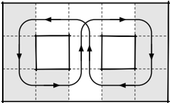
Suppose you want to study how an animal, when presented with two options A and B, can learn to alternatively choose A then B then A, etc. One typical lab setup to study such alternate decision task is the T-maze environment where the animal is confronted to a left or right turn and can be subsequently trained to display an alternate choice behavior. This task can be easily formalized using a block world as it is regularly done in the computational literature. Using such formalization, a simple solution is to negate (logically) a one bit memory each time the model reaches A or B such that, when located at the choice point, the model has only to read the value of this memory in order to decide to go to A or B. However, as simple as it is, this abstract formalization entails the elaboration of an explicit internal representation keeping track of the recent behavior, implemented in a working memory that can be updated when needed. But then, what could be the alternative? Let us consider a slightly different setup where the T-Maze is transformed into a closed 8-Maze (see figure 1-Left). Suppose that you can only observe the white area when the animal is evolving along the arrowed line (both in observable and non-observable areas). From the observer point of view, the animal is turning left one time out of two and turning right one time out of two. Said differently, the observer can infer an alternating behavior because of its
Karen Sobriel
Inria Bordeaux Sud-Ouest
Univ. Bordeaux, CNRS
Nicolas Rougier Inria Bordeaux Sud-Ouest Univ. Bordeaux, CNRS
<details>
<summary>Image 1 Details</summary>
### Visual Description
## Diagram: Interconnected Cyclical System
### Overview
The image depicts a schematic diagram of two interconnected square components arranged horizontally. Arrows form a continuous loop around and between the squares, suggesting a cyclical or feedback-driven process. The background is divided into light gray and white vertical sections by dashed lines. No textual labels, legends, or numerical data are present.
### Components/Axes
- **Primary Elements**:
- Two identical square shapes positioned side-by-side.
- Arrows forming a closed loop:
- Outer arrows circulate clockwise around the perimeter of both squares.
- Inner arrows connect the squares bidirectionally (upward and downward).
- Dashed vertical lines segment the background into five equal-width columns.
- **Color Scheme**:
- Squares and arrows: Black.
- Background: Alternating light gray and white vertical stripes.
### Detailed Analysis
- **Spatial Grounding**:
- Squares are centered horizontally within the diagram.
- Arrows are evenly spaced along their paths, with no overlap or deviation.
- Dashed lines run vertically from top to bottom, dividing the diagram into five equal sections.
- **Flow Direction**:
- Outer loop: Clockwise circulation around the entire structure.
- Inner loop: Bidirectional arrows between the squares (top and bottom).
- **Absence of Text**:
- No labels, legends, or annotations are visible.
- No numerical values, units, or categorical identifiers are present.
### Key Observations
1. The diagram emphasizes symmetry and cyclicality, with no discernible start or end point.
2. The bidirectional inner arrows suggest mutual interaction or exchange between the two squares.
3. The dashed lines may imply segmentation or modularity in the system.
### Interpretation
This diagram likely represents a theoretical or abstract model of a system with reciprocal dependencies. The interconnected squares could symbolize two entities (e.g., processes, departments, or components) engaged in a continuous exchange, while the outer loop reinforces the cyclical nature of the process. The lack of labels or data points suggests the diagram is conceptual rather than data-driven, focusing on structural relationships rather than quantitative analysis. The bidirectional inner arrows highlight interdependence, whereas the outer loop underscores systemic continuity.
</details>
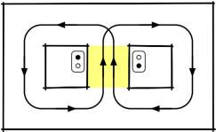
Fig. 1. Left: An expanded view of a T-Maze. An observer can infer an alternating behavior because of her partial view (white area) of the system. Right: 8-maze with cues. A cue (left or right) is given only when the bot is present inside the yellow area.
<details>
<summary>Image 2 Details</summary>
### Visual Description
## Diagram: Bidirectional System Interaction Model
### Overview
The image depicts a technical diagram illustrating bidirectional interactions between two interconnected systems or components. Arrows form closed loops around each component, with a highlighted yellow area indicating a critical interface or interaction zone between them.
### Components/Axes
- **Left Rectangle**: Contains two symbols:
- A filled black circle (●)
- An outlined white circle (○)
- **Right Rectangle**: Contains two outlined white circles (○)
- **Arrows**:
- Bidirectional arrows connect the two rectangles, forming continuous loops.
- Arrows are black with arrowheads, indicating directional flow.
- **Highlighted Area**: A yellow-shaded region between the rectangles, emphasizing the interaction zone.
### Detailed Analysis
- **Left Component Symbols**:
- Filled circle (●): Likely represents a primary state or active element.
- Outlined circle (○): May denote a secondary state or passive element.
- **Right Component Symbols**:
- Two outlined circles (○, ○): Suggests dual passive or secondary states.
- **Flow Dynamics**:
- Bidirectional arrows imply mutual exchange or synchronization between components.
- Closed loops suggest cyclical processes or feedback mechanisms.
### Key Observations
1. The highlighted yellow area between the rectangles is the only visually distinct element, suggesting its functional importance.
2. The left component has one active (●) and one passive (○) element, while the right component has two passive elements (○, ○).
3. No numerical data, labels, or legends are present in the diagram.
### Interpretation
This diagram likely represents a system architecture where two components interact bidirectionally. The left component may have a primary-active state (●) and a secondary state (○), while the right component operates in dual passive states. The highlighted yellow interface implies a critical point for data exchange, control signals, or synchronization. The absence of labels necessitates further context to confirm the exact nature of the components (e.g., hardware modules, software processes, or biological systems). The bidirectional loops suggest a closed-loop system with feedback, common in control systems, communication protocols, or coupled mechanical/electrical systems.
</details>
partial view of the system. The question is: does the animal really implement an explicit alternate behavior or is it merely following a mildly complex dynamic path? This is not a rhetorical question because depending on your hypothesis, you may search for neural correlates that actually do not exist. Furthermore, if the animal is following such mildly complex dynamic path, does this mean that it has no explicit access to (not to say no consciousness of) its own alternating behavior?
This question is tightly linked to the distinction between implicit learning (generally presented as sub-symbolic, associative and statistics-based) and explicit learning (symbolic, declarative and rule-based). Implicit learning refers to the nonconscious effects that prior information processing may exert on subsequent behavior [1]. It is implemented in associative sensorimotor procedural learning and also in model-free reinforcement learning, with biological counterparts in the motor and premotor cortex and in the basal ganglia. Explicit learning is associated with consciousness or awareness, and to the idea of building explicit mental representations [2] that can be used for flexible behavior, involving the prefrontal cortex and the hippocampus. This is what is proposed in model-based reinforcement learning and in other symbolic approaches for planning and reasoning. These strategies of learning are not independent but their relations and interdependencies are not clear today. Explicit learning is often observed in the early stages of learning whereas implicit learning appears on the long run, which can be explained as a way to decrease the cognitive load. But there is also a body of evidence, for example in sequence learning [3] or artificial grammar learning studies [4], that suggests that explicit learning is not a mandatory early step and that improvement in task performance are not necessarily accompanied by the ability to express the acquired knowledge in an explicit way [5].
Coming back to the task mentioned above, it is consequently not clear if we can learn rules without awareness and then to what extent can such implicit learning be projected to performance in an unconscious way? Furthermore, without turning these implicit rules into an explicit mental representation, is it possible to manipulate the rules, which is a fundamental trademark of flexible adaptable control of behavior?
Using the reservoir computing framework generally considered as a way to implement implicit learning, we first propose that a simple alternation or sequence learning task can be solved without an explicit pre-encoded representation of memory. However, to then be able to generate a new sequence or manipulate the rule learnt, we explain that inserting explicit cues in the decision process is needed. In a second series of experiments, we provide a proof of concept still using the reservoir computing framework, for the hypothesis that the recurrent network forms contextual representations from implicitly acquired rules over time. We then show that these representations can be considered explicit and necessary to be able to manipulate behaviour in a flexible manner.
In order to provide preliminary interpretation of what is observed here, it is reminded that recurrent networks, particularly models using the reservoir computing framework, are a suitable candidate to model the prefrontal cortex [6], also characterized by local and recurrent connections. Given their inherent sensitivity to temporal structure, it also makes these networks adaptable for sequence learning. This approach has been used to model complex sensorimotor couplings [7] from the egocentric view of an agent (or animal) that is situated in its environment and can autonomously demonstrate reactive behaviour from its sensory space [8], as we also do in the first series of experiments, for learning sensorimotor couplings by demonstration, or imitation. In the second series of experiment, we propose that the prefrontal cortex is the place where explicit representations can be elaborated when flexible behaviors are required.
## II. METHODS AND TASK
The objective is the creation of a reservoir computing network of type Echo State Network (ESN) that controls the movement of a robot [8], [9], which has to solve a decision-making task (alternately going right and left at an intersection) in the maze presented in figure 1.
## A. Model Architecture : Echo State Network
An ESN is a recurrent neural network (called reservoir) with randomly connected units, associated with an input layer and an output layer, in which only the output (also called readout) neurons are trained. The neurons have the following dynamics:
$$\begin{array} { r l r } { x [ n ] } & = } & { ( 1 - \alpha ) x [ n - 1 ] + \alpha \tilde { x } [ n ] } & { ( 1 ) } \end{array}$$
$$\begin{array} { r l r } { \tilde { x } [ n ] } & = } & { \tanh ( W x [ n - 1 ] + W _ { i n } [ 1 ; u [ n ] ] ) } & { ( 2 ) } \end{array}$$
$$\begin{array} { r l r } { y [ n ] } & { = } & { f ( W _ { o u t } [ 1 ; \tilde { x } ( n ) ] ) } & { ( 3 ) } \end{array}$$
where x ( n ) is a vector of neurons activation, ˜ x ( n ) its update, u ( n ) and y ( n ) are respectively the input and the output vectors, all at time n . W , W in , W out are respectively the reservoir, the input and the output weight matrices. The notation [ . ; . ] stands for the concatenation of two vectors. α corresponds to the leak rate. tanh corresponds to the hyperbolic tangent function and f to linear or piece-wise linear function.
The values in W , W in , W out are initially randomly chosen. While W , W in are kept fixed, the output weights W out are the only ones plastic (red arrows in Figure 2). In this model, the output weights are learnt with the ridge regression method (also known as Tikhonov regularization):
$$W _ { o u t } = Y ^ { t \arg e t } X ^ { T } ( X X ^ { T } + \beta I ) ^ { - 1 } \quad ( 4 )$$
where Y target is the target signal to approximate, X is the concatenation of 1, the input and the neurons activation vectors: [1; u ( n ); x ( n )] , β corresponds to the regularization coefficient and I the identity matrix.
## B. Experiment 1 : Uncued sequence learning
The class of tasks called spatial alternation has been widely used to study hippocampal and working memory functions [10]. For the purpose of our investigation, we simulated a continuous version of the same task, wherein the agent needs to alternate its choice at a decision point, and after the decision, it is led back to the central corridor, in essence following an 8shaped trace while moving (see figure 1-Left). This alternation task is widely believed to require a working memory such as to remember what was the previous choice in order to alternate it. Here we show that the ESN previously described is sufficient to learn the task without an explicit representation of the memory.
1) Tutor model: In order to generate data for learning, we implemented a simple Braintenberg vehicle where the robot moves automatically with a constant speed and changes its orientation according to the values of its sensors. At each time step the sensors measure the distance to the walls and the bot turns such as to avoid the walls. At each timestep, the position of the bot is updated as follows:
$$\begin{array} { r l r } { s k } & \quad } \\ { z e } & \quad } \\ { ( 5 ) } \end{array}$$
$$\begin{array} { r l r } { p ( n ) } & = } & { p ( n - 1 ) + 2 * \left ( \cos ( \theta ( n ) ) + \sin ( \theta ( n ) ) \right ) } & { ( 6 ) } \end{array}$$
where p ( n ) and p ( n +1) are the positions of the robot at time step n and n +1 , θ ( n ) is the orientation of the robot, calculated as the weighted sum ( α i ) of the values of the sensors s i . The norm of the movement is kept constant and fixed at 2.
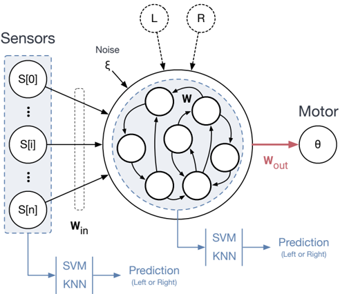
Fig. 2. Model Architecture with 8 sensor inputs, and a motor output (orientation). The black arrows are fixed while the red arrows are plastic and are trained. The reservoir states are used as the input to a classifier which is trained to make a prediction about the decision (going left or right) of the robot. A left (L) and right (R) cue can be fed to the model depending on the experiment (see Methods).
<details>
<summary>Image 3 Details</summary>
### Visual Description
## Diagram: Sensor-Motor Control System with Machine Learning Processing
### Overview
This diagram illustrates a closed-loop control system integrating sensor data, machine learning processing, and motor actuation. The system processes sensor inputs through a computational unit (CPU) containing SVM and KNN models to predict directional decisions (Left/Right), which then control motor movement. Key components include noise injection (ξ), internal weights (w), and output angle (θ).
### Components/Axes
1. **Left Section (Sensors)**:
- Vertical array of labeled sensor inputs: S[0], S[1], ..., S[n]
- Dashed vertical line indicates noise injection point (ξ)
2. **Central Processing Unit (CPU)**:
- Circular boundary containing:
- Internal weights (w) connecting sensor inputs to processing nodes
- Two output arrows labeled "L" (Left) and "R" (Right)
- Dashed boundary indicating processing boundaries
3. **Right Section (Motor)**:
- Output angle (θ) connected to motor
- Weighted output (W_out) in red
4. **Arrows and Flow**:
- Black arrows show data flow from sensors → CPU → motor
- Red arrow specifically highlights motor output (W_out)
### Detailed Analysis
- **Sensor Inputs**:
- Multiple discrete sensors (S[0] to S[n]) provide input data
- Noise (ξ) injected at sensor level before processing
- **CPU Processing**:
- Contains weighted connections (w) between sensor inputs and processing nodes
- Implements two machine learning models:
- SVM KNN (Support Vector Machine + K-Nearest Neighbors)
- Prediction outputs: Left or Right decisions
- Internal processing represented by interconnected nodes
- **Motor Output**:
- Final output angle (θ) controlled by weighted output (W_out)
- Red arrow emphasizes actuation pathway
### Key Observations
1. System architecture follows sensor → processing → actuation flow
2. Dual machine learning models (SVM and KNN) used for directional prediction
3. Noise injection occurs at the sensor level before processing
4. Output angle (θ) is directly controlled by weighted output (W_out)
5. No explicit numerical values provided in diagram
### Interpretation
This diagram represents a hybrid control system combining traditional sensorimotor control with modern machine learning techniques. The integration of SVM and KNN suggests a probabilistic approach to directional decision-making, likely for applications requiring adaptive movement control (e.g., robotics, autonomous systems). The noise injection (ξ) indicates awareness of real-world sensor imperfections, while the weighted connections (w) imply learnable parameters that could be optimized through training. The dual output arrows (L/R) suggest binary decision-making capability, with the motor's angle (θ) representing continuous control output. The system's closed-loop nature implies potential for feedback mechanisms not explicitly shown in this diagram.
</details>
Fig. 3. Generation of the 8-shape pathway with the addition of walls at the intersection points
<details>
<summary>Image 4 Details</summary>
### Visual Description
## Diagram: Robot Pathfinding Simulation in Grid Environment
### Overview
The image depicts a four-panel sequence illustrating a robot's movement and pathfinding in a grid-based environment. Each panel shows a 2x2 grid with two shaded squares (obstacles) and a dotted path representing the robot's trajectory. Red lines indicate directional movement or sensor rays.
### Components/Axes
- **Grid Layout**:
- 2x2 grid in each panel, divided into four equal squares.
- Two squares are shaded (black grid patterns), representing obstacles.
- Dotted paths (gray) show the robot's movement history.
- Red lines represent instantaneous movement or sensor activation.
- **Robot**:
- Circular shape with radiating lines (sensors) in some panels.
- Positioned at grid intersections or mid-grid points.
- **Pathfinding Elements**:
- Dotted paths vary in complexity across panels, suggesting iterative path adjustments.
- Red lines originate from the robot, indicating directional decisions.
### Detailed Analysis
- **Panel 1 (Top-Left)**:
- Robot starts at the bottom-left grid intersection.
- Dotted path curves upward, avoiding the top-left obstacle.
- Red line extends diagonally toward the top-right obstacle.
- **Panel 2 (Top-Right)**:
- Robot moves to the top-right grid intersection.
- Dotted path loops around the top-left obstacle.
- Red line extends horizontally leftward.
- **Panel 3 (Bottom-Left)**:
- Robot positioned at the bottom-right grid intersection.
- Dotted path loops around the bottom-left obstacle.
- Red line extends diagonally upward-left.
- **Panel 4 (Bottom-Right)**:
- Robot at the center of the grid.
- Dotted path forms a complex loop around both obstacles.
- Red line extends horizontally rightward.
### Key Observations
1. **Pathfinding Strategy**:
- The robot avoids obstacles by adjusting its trajectory, as shown by the dotted paths.
- Red lines suggest real-time sensor feedback influencing movement decisions.
2. **Grid Symmetry**:
- Obstacles are consistently placed in the top-left and bottom-right squares across all panels.
3. **Sensor Coverage**:
- Radiating lines (sensors) in Panels 2 and 4 indicate omnidirectional awareness.
### Interpretation
The diagram demonstrates a reactive pathfinding algorithm where the robot dynamically adjusts its route based on obstacle detection. The red lines likely represent sensor-triggered movements, while the dotted paths visualize historical trajectories. The consistent obstacle placement suggests a controlled environment for testing navigation strategies. No numerical data or textual labels are present, so quantitative analysis is not applicable.
</details>
- 2) Training data: The ESN is trained using supervised learning, containing samples from the desired 8-shaped trajectory. Since the Braitenberg algorithm only aims to avoid obstacles, the robot is forced into the desired trajectory by adding walls at the intersection points as shown in figure 3. After generating the right pathway, the added walls are removed and the true sensor values are gathered as input. Gaussian noise is added to the position values of the robot at every time step in order to make the training more robust. Approximately 50,000 time steps were generated (equivalent to 71 complete 8-loops) and separated into training and testing sets.
3) Hyper parameters tuning: The ESN was built with the python library ReservoirPy [11] with the hyper-parameters presented in table I, column 'Without context'. The order
| Parameter | Without context | With context |
|------------------------|-------------------|----------------------------|
| Input size | 8 | 10 |
| Output size | 1 | 1 |
| Number of units | 1400 | 1400 |
| Input connectivity | 0.2 | 0.2 |
| Reservoir connectivity | 0.19 | 0.19 |
| Reservoir noise | 0.01 | 1e-2 |
| Input scaling | 1 | 1(sensors), 10.4695 (cues) |
| Spectral Radius | 1.4 | 1.505 |
| Leak Rate | 0.0181 | 0.06455 |
| Regularization | 4.1e-08 | 1e-3 |
TABLE I
PARAMETER CONFIGURATION FOR THE ESN
of magnitude of the hyper-parameters was first found using the Hyperopt python library [12], then these were fine tuned manually. The ESN receives as input the values of the 8 sensors and output the next orientation.
4) Model evaluation: The performance of the ESN has been calculated with the Normalized Root Mean Squared Error metrics ( NRMSE ) and the R square ( R 2 ) metrics, defined as follows :
$$N R M S E = \frac { \sqrt { \frac { \sum _ { i = 1 } ^ { n } ( y _ { i } - \hat { y } _ { i } ) ^ { 2 } } { n } } } { \sigma } \quad ( 7 )$$
$$R ^ { 2 } = 1 - \frac { \sum ( y _ { i } - \hat { y } _ { i } ) ^ { 2 } } { \sum ( y _ { i } - \bar { y } ) ^ { 2 } } \quad ( 8 )$$
where y i , ˆ y i and ¯ y are respectively the desired output, the predicted output and the mean of the desired output.
5) Reservoir state analysis: In this section the reservoir states are analysed such as to inspect to which extent they form an internal and hidden representation of the memory. To do so, we use Principal Component Analysis (PCA), a dimensionality reduction method enabling the identification of patterns and important features of the processed data. PCA is carried out on the reservoir states for each position of the robot during the 8-shape trajectory. We continued the analysis by doing a classification of the reservoir states. We made the assumption that it is possible to know the future direction of the robot observing the internal states of the reservoir. This implies that the reservoir states can be classified in two classes: one related to the prediction of going left and the other related to the prediction of going right. Two standard classifiers, the KNN (K-Nearest Neighbors) and the SVM (Support Vector Machine) were used. They take as input the reservoir state at each position of the bot while executing the 8-shape and predict the decision the robot will take at the next intersection (see figure 2). Since the classifiers are trained using supervised learning, the training data were generated in the central corridor of the maze (yellow area in figure 1Right), assuming that it is where the reservoir is in the state configuration in which it already knows which direction it will take at the next intersection. 900 data points were generated and separated into training and testing sets.
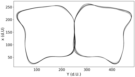
Fig. 4. The trajectory of the robot following the 8-trace in the cartesian map.
<details>
<summary>Image 5 Details</summary>
### Visual Description
## Line Graph: Cyclical Data Series Overlapping in Y-Axis Range
### Overview
The image depicts a line graph with two overlapping closed-loop trajectories plotted against a Cartesian coordinate system. The graph shows cyclical patterns with distinct peaks and troughs, suggesting periodic or oscillatory behavior in the data. The loops intersect spatially but lack explicit numerical annotations or legends.
### Components/Axes
- **X-Axis (Horizontal)**: Labeled "Y (d.U.)" with a scale from 100 to 400 in increments of 100.
- **Y-Axis (Vertical)**: Labeled "x (d.U.)" with a scale from 50 to 250 in increments of 50.
- **Lines**: Two continuous black lines forming closed loops. No legend or color-coding is present to differentiate the lines.
- **Overlap Region**: The loops intersect between Y=200–300 (d.U.) and x=150–200 (d.U.).
### Detailed Analysis
1. **Left Loop**:
- Starts at approximately (Y=100, x=50).
- Peaks at (Y=200, x=250).
- Returns to the starting point, forming a counterclockwise loop.
- Exhibits a smooth, symmetrical arc with minimal deviation.
2. **Right Loop**:
- Begins at (Y=300, x=50).
- Peaks at (Y=400, x=250).
- Returns to the starting point, forming a clockwise loop.
- Mirrors the left loop’s shape but is offset along the Y-axis.
3. **Overlap**:
- Both loops intersect in the central region (Y=200–300, x=150–200).
- The overlapping area suggests a shared range of values where the two data series converge.
### Key Observations
- **Symmetry**: Both loops exhibit near-identical amplitude (x=50–250) but differ in Y-axis positioning.
- **Peak Alignment**: The maximum x-values (250) occur at Y=200 (left loop) and Y=400 (right loop), indicating a potential relationship between Y and x at critical points.
- **No Numerical Labels**: Data points lack explicit values, making precise quantification impossible.
- **Ambiguous Units**: "d.U." is undefined, limiting interpretation of scale.
### Interpretation
The graph likely represents two cyclical processes or variables with similar magnitudes but distinct Y-axis dependencies. The overlapping region implies a shared operational range where both processes interact or coexist. The absence of legends or numerical annotations prevents definitive conclusions about causality or correlation. The mirrored symmetry suggests a designed or natural balance between the two series, possibly indicating redundancy, competition, or complementary dynamics. Further context (e.g., data source, units) is required to validate hypotheses about the system’s behavior.
</details>
## C. Experiment 2 : 8 Maze Task with Contextual Inputs
In this experiment, we fed the reservoir with two additional inputs that represent the next decision, one being related to a right turn (R) and the other to a left turn (L) (see figure 2). They are binary values, switched to a value of 1 only when the bot is known to take the corresponding direction. We thus built a second ESN with the hyper-parameters presented in TABLE I, column 'With context'. The network is similar to the previous one, except that the contextual inputs are added with a different input scaling than the one used for the sensors inputs. During the data generation, the two additional inputs are set to 0 everywhere in the maze, except in the central corridor.
## III. RESULTS
## A. Motor sequence learning
We first show that a recurrent neural network like the ESN can learn a rule-based trajectory in the continuous space, without an explicit memory or feedback connections. The score of the ESN is shown in TABLE II and the results for the trajectory predicted by the ESN are presented in figure 4 and in the top panel in figure 8. At each period of about 350 steps, a behavior or decision switch takes place, which is evident from the crests and troughs in the y-axis coordinates. It can be seen that the ESN correctly predicts the repeated alternating choice in the central arm of the maze. In addition to switching between the left and right loops, the robot also moves through the environment without colliding into obstacles.
| Performance of the ESN for 50 simulations | Performance of the ESN for 50 simulations | Performance of the ESN for 50 simulations | Performance of the ESN for 50 simulations |
|---------------------------------------------|---------------------------------------------|---------------------------------------------|---------------------------------------------|
| NRMSE | NRMSE | R 2 | R 2 |
| Mean | 0.0171 | Mean | 0.9962 |
| Variance | 5.4466e-06 | Variance | 1.0192e-06 |
TABLE II
NRMSE AND R 2 SCORE OF THE ESN WITH 8 INPUTS
## B. Reservoir State Prediction
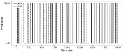
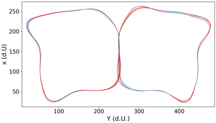
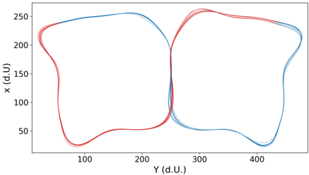
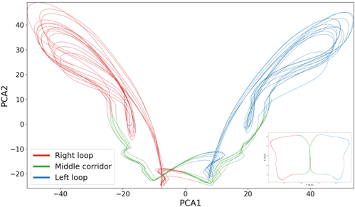
Next, we show that even a simple classifier such as SVM or KNN can observe the internal states of the reservoir and learn to predict the decision (whether to go left or right) of the network. The results of the predictions are presented in the top part of figure 5. As expected, there is a periodicity of choice in line with the position of the bot in the maze, showing that the classification is relevant. At each time step, both classifiers output the same prediction with a small discrepancy in time. The accuracy score obtained for both classifiers is 1. In the bottom part of figure 5, we can observe that the robot knows quite early which decision it will take at the next loop while we could expect that it would take its decision in the yellow corridor in figure 1. Here, we see that if the robot just turned right, the reservoir switches its internal state to go left next time only a few dozen time steps after. We tried the same classifiers but instead of the reservoir states as input, we used the sensors values. The results are shown in the figure 5. As expected, the classifications fail with an accuracy score of 0.57 for SVM and 0.43 for KNN; this randomness can be seen in both figures. Thus, we showed that by simply observing the internal states of the reservoir, it is possible to predict its next prediction. In essence, this is a proof of concept to show that second-order or observer networks, mimicking the role of the regions of the prefrontal cortex implementing contextual rules, can consolidate information linking sensory information to motor actions, to develop relevant contextual representations. Since the state space of the dynamic reservoir is highdimensional, using the Principal Component Analysis (PCA) on the states, we investigated if it is possible to observe subspace attractors. The result for the PCA analysis is presented in figure 7, where PCA was applied for 5000 time steps, which corresponds to 7 8-loops. The figure shows two symmetric sub-attractors, which are linearly separable, that correspond to the two parts of the 8-shape trajectory.
## C. Explicit rules with contextual inputs
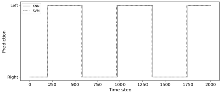
Finally, we demonstrate that although the ESN can learn a motor sequence without contextual inputs, it is limited by its internal representation to learn more complex sequences which may require a longer memory. Adding contextual or explicit information about the rule (which we propose are representations developed by the prefrontal cortex over time) can then bias the ESN to follow any arbitrary trajectory as in 8. With the additional contextual inputs, the ESN is able to reproduce the standard 8 sequence (the performance is shown in table III) but can also achieve more complex tasks by sending to it the proper contextual inputs. One example can be seen in figure 8: the top graph shows the positions of the bot while making the standard 8 sequence [ABABABAB...], the bottom one shows that the bot was able to achieve a more complex sequence [AABBAABBAABB...].
## IV. DISCUSSION
Using a simple reservoir model that learns to follow a specific path, we have shown how the resulting behavior could be
<details>
<summary>Image 6 Details</summary>
### Visual Description
## Bar Chart: Prediction Comparison Between KNN and SVM Over Time Steps
### Overview
The image is a bar chart comparing the performance of two machine learning models, K-Nearest Neighbors (KNN) and Support Vector Machines (SVM), across 2000 time steps. The chart uses vertical bars to represent predictions, with two distinct patterns for each model: solid lines for KNN and dotted lines for SVM. The y-axis is labeled "Prediction" with two categories: "Left" (bottom) and "Right" (top). The x-axis represents time steps, incrementing in intervals of 250 from 0 to 2000.
### Components/Axes
- **X-axis (Horizontal)**: Labeled "Time step," with markers at 0, 250, 500, 750, 1000, 1250, 1500, 1750, and 2000.
- **Y-axis (Vertical)**: Labeled "Prediction," with two categories:
- "Left" (bottom)
- "Right" (top)
- **Legend**: Located in the top-left corner, with:
- **KNN**: Solid black bars
- **SVM**: Dotted gray bars
### Detailed Analysis
- **KNN (Solid Bars)**:
- Consistently taller than SVM bars across all time steps.
- Dominates the "Right" category in most intervals, with occasional dominance in "Left" near time steps 0 and 2000.
- No visible gaps or missing data points.
- **SVM (Dotted Bars)**:
- Shorter than KNN bars in all intervals.
- Predominantly occupies the "Left" category, with minimal presence in "Right."
- Uniform pattern across all time steps.
### Key Observations
1. **Model Performance**: KNN consistently outperforms SVM in prediction frequency, as evidenced by taller bars.
2. **Temporal Stability**: Both models show no significant deviation in performance across time steps, suggesting stable behavior.
3. **Category Distribution**: KNN favors the "Right" prediction, while SVM is skewed toward "Left."
### Interpretation
The chart demonstrates that KNN is more effective than SVM for this specific task, likely due to its ability to capture local patterns in the data. The lack of temporal variation implies that neither model experiences concept drift over time. The stark contrast in bar heights suggests a potential imbalance in class distribution or a fundamental difference in model architecture suitability for the problem. Further investigation into feature engineering or hyperparameter tuning for SVM could bridge this performance gap.
</details>
<details>
<summary>Image 7 Details</summary>
### Visual Description
## Line Graph: Path Trajectories Comparison
### Overview
The image depicts a line graph with two intersecting loops representing two distinct paths (red and blue). The graph spans a coordinate system with X (d.U.) and Y (d.U.) axes, where "d.U." likely denotes "deci-units" or a domain-specific measurement. The red and blue lines form mirrored, figure-eight-like trajectories that intersect near the center of the graph.
### Components/Axes
- **X-axis (Horizontal)**: Labeled "Y (d.U.)", scaled from 0 to 400 in increments of 100.
- **Y-axis (Vertical)**: Labeled "X (d.U.)", scaled from 0 to 250 in increments of 50.
- **Legend**: Located in the top-right corner, associating:
- **Red line**: "Path A"
- **Blue line**: "Path B"
### Detailed Analysis
1. **Path A (Red Line)**:
- Starts at approximately (50, 50).
- Rises sharply to a peak near (250, 250).
- Descends diagonally to a trough at (350, 50).
- Forms a clockwise loop intersecting Path B at (250, 125).
2. **Path B (Blue Line)**:
- Starts at approximately (50, 200).
- Descends to a trough near (250, 50).
- Rises diagonally to a peak at (350, 200).
- Forms a counterclockwise loop intersecting Path A at (250, 125).
3. **Intersection Point**:
- Both paths cross at (250, 125), forming an "X" shape.
- The red line dominates the upper-right quadrant, while the blue line dominates the lower-left.
### Key Observations
- **Symmetry**: The paths exhibit mirrored behavior, suggesting a balanced or reciprocal relationship.
- **Intersection Significance**: The crossing at (250, 125) may represent a critical junction or equilibrium point.
- **Loop Dynamics**: Both paths complete a single loop, indicating cyclical or periodic behavior.
### Interpretation
The graph likely models two competing or complementary processes (e.g., opposing forces, dual trajectories) that intersect at a shared reference point. The symmetry implies a designed balance, while the intersection could signify a convergence of goals, resources, or states. The loops suggest cyclical activity, possibly representing periodic events or feedback mechanisms. The absence of additional data points or annotations leaves the exact context ambiguous, but the structure hints at a system where dual trajectories interact dynamically.
</details>
Fig. 5. Prediction from sensors during 2000 time steps. Top figure shows the prediction of the KNN and SVM classifier, bottom figure shows the SVM prediction along the trajectory.
| Performance of the ESN for 50 runs | Performance of the ESN for 50 runs | Performance of the ESN for 50 runs | Performance of the ESN for 50 runs |
|--------------------------------------|--------------------------------------|--------------------------------------|--------------------------------------|
| NRMSE | NRMSE | R 2 | R 2 |
| Mean | 0.0050 | Mean | 0.9997 |
| Variance | 1.1994e-07 | Variance | 2.0220e-09 |
TABLE III
NRMSE AND R 2 SCORE OF THE ESN WITH THE TWO ADDITIONAL CONTEXTUAL INPUTS
interpreted as an alternating behavior by an external observer. However, we've also shown that from the point of view of the model and in the absence of associated cues, this behavior cannot be interpreted as such. Instead, the behavior results from the internal dynamics of the reservoir (and the learning procedure we implemented). Without external cues, the model is unable to escape its own behavior and is trapped inside an attractor. Only the cues can provide the model with the necessary and explicit information that in turn allows to bias its behavior in favor of option A or option B.
From a neuroscience perspective, as developed in more details in [13], it can be proposed that the reservoir model in the first experiment implements the premotor cortex learning sensorimotor associations in the anterior cortex. In the first experiment, this is made by supervised learning in a process of learning by imitation. In a different protocol, this is also classically be done by reinforcement learning, involving another region of the anterior cortex, the anterior cingulate cortex,
<details>
<summary>Image 8 Details</summary>
### Visual Description
## Line Graph: Prediction Behavior of KNN and SVM Models Over Time
### Overview
The image is a line graph comparing the prediction behavior of two machine learning models (KNN and SVM) across 2000 time steps. The y-axis represents binary prediction categories ("Left" and "Right"), while the x-axis represents sequential time steps. Two distinct data series are plotted: a solid line for KNN and a dotted line for SVM.
### Components/Axes
- **X-axis (Horizontal)**:
- Label: "Time step"
- Scale: 0 to 2000 in increments of 250
- Position: Bottom of the graph
- **Y-axis (Vertical)**:
- Label: "Prediction"
- Categories: "Left" (bottom) and "Right" (top)
- Position: Left side of the graph
- **Legend**:
- Position: Top-left corner
- Entries:
- Solid line: "KNN"
- Dotted line: "SVM"
### Detailed Analysis
1. **KNN Model (Solid Line)**:
- **Initial State**: Predicts "Left" from time step 0 to ~250.
- **First Switch**: Transitions to "Right" at ~250, maintaining this prediction until ~750.
- **Second Switch**: Returns to "Left" at ~750, lasting until ~1250.
- **Third Switch**: Shifts to "Right" at ~1250, persisting until ~1750.
- **Final State**: Reverts to "Left" at ~1750, ending at time step 2000.
- **Key Pattern**: Alternates predictions every ~500 time steps, with the final prediction being "Left".
2. **SVM Model (Dotted Line)**:
- **Initial State**: Predicts "Left" from time step 0 to ~500.
- **First Switch**: Transitions to "Right" at ~500, maintaining this until ~1000.
- **Second Switch**: Returns to "Left" at ~1000, lasting until ~1500.
- **Third Switch**: Shifts to "Right" at ~1500, continuing until time step 2000.
- **Key Pattern**: Alternates predictions every ~500 time steps, with the final prediction being "Right".
### Key Observations
- **Temporal Consistency**: Both models exhibit periodic prediction switches, but with differing frequencies and durations.
- **Final Prediction Divergence**: At time step 2000, KNN predicts "Left" while SVM predicts "Right", indicating model-specific final states.
- **Switch Timing**:
- KNN switches at ~250, 750, 1250, 1750.
- SVM switches at ~500, 1000, 1500.
- **Stability**: SVM maintains predictions for longer intervals (500 steps) compared to KNN's shorter intervals (~250–500 steps).
### Interpretation
The graph demonstrates contrasting prediction dynamics between KNN and SVM:
1. **KNN Behavior**:
- Suggests higher sensitivity to recent data, as evidenced by more frequent prediction changes.
- Final "Left" prediction at 2000 may reflect recent input patterns dominating its output.
2. **SVM Behavior**:
- Indicates greater stability, with predictions persisting for longer intervals.
- Final "Right" prediction at 2000 suggests reliance on broader temporal context rather than recent data.
3. **Practical Implications**:
- KNN might be more suitable for applications requiring rapid adaptation to new data.
- SVM could be preferable for scenarios demanding consistent, long-term predictions.
4. **Anomalies**:
- The abrupt switch at time step 1750 for KNN (from Right to Left) deviates from its earlier ~500-step intervals, potentially indicating an outlier or data shift.
### Spatial Grounding
- **Legend**: Top-left corner, clearly associating line styles with model names.
- **Y-axis Categories**: "Left" positioned at the bottom, "Right" at the top, creating a vertical binary distinction.
- **X-axis Markers**: Time steps labeled at 0, 250, 500, ..., 2000, with grid lines for reference.
### Content Details
- **Numerical Values**:
- KNN switches: ~250, 750, 1250, 1750.
- SVM switches: ~500, 1000, 1500.
- **Line Styles**: Solid (KNN) vs. Dotted (SVM) for visual differentiation.
### Conclusion
The graph highlights model-specific prediction strategies, with KNN favoring recent data and SVM emphasizing stability. These differences underscore the importance of model selection based on application requirements for temporal sensitivity versus consistency.
</details>
Time step
Fig. 6. Prediction from reservoir state during 2000 time steps. Top figure shows the predictions of the KNN and SVM classifier. Bottom figure shows the SVM prediction along the trajectory.
<details>
<summary>Image 9 Details</summary>
### Visual Description
## Line Graph: Intersecting Loops of Line A and Line B
### Overview
The image depicts a line graph with two distinct loops (red and blue) plotted on a coordinate plane. The red line (Line A) and blue line (Line B) form closed loops that intersect near the center of the graph. The axes are labeled with "X (d.U.)" and "Y (d.U.)", suggesting a coordinate system with units denoted as "d.U." (possibly a domain-specific unit).
### Components/Axes
- **X-axis**: Labeled "Y (d.U.)", ranging approximately from 50 to 400.
- **Y-axis**: Labeled "X (d.U.)", ranging approximately from 50 to 250.
- **Legend**: Located in the top-right corner, with:
- **Red**: "Line A"
- **Blue**: "Line B"
### Detailed Analysis
- **Line A (Red)**:
- Starts at the bottom-left corner (X ≈ 50, Y ≈ 100).
- Rises to the top-left (X ≈ 250, Y ≈ 250).
- Moves right to the top-right (X ≈ 400, Y ≈ 250).
- Descends to the bottom-right (X ≈ 400, Y ≈ 50).
- Returns to the starting point, forming a loop.
- **Line B (Blue)**:
- Starts at the bottom-right corner (X ≈ 400, Y ≈ 50).
- Rises to the top-right (X ≈ 400, Y ≈ 250).
- Moves left to the top-left (X ≈ 250, Y ≈ 250).
- Descends to the bottom-left (X ≈ 50, Y ≈ 100).
- Returns to the starting point, forming a loop.
- **Intersection**: The two lines intersect near the center of the graph at approximately (X ≈ 250, Y ≈ 200).
### Key Observations
1. **Symmetry**: The loops are roughly symmetrical but not perfectly aligned.
2. **Intersection Point**: The crossing of Line A and Line B suggests a shared reference or equilibrium point.
3. **Axis Labeling**: The X-axis is labeled "Y (d.U.)" and the Y-axis "X (d.U.)", which may indicate a non-standard coordinate system or a potential labeling error.
4. **Unit Ambiguity**: The unit "d.U." is undefined in the image, requiring further context for interpretation.
### Interpretation
The graph likely represents two cyclical processes or variables (Line A and Line B) that interact at a central point. The loops could symbolize recurring patterns, feedback mechanisms, or interdependent systems. The intersection at (250, 200) may indicate a critical threshold or equilibrium state where the two processes converge. The axis labeling discrepancy ("X" vs. "Y") raises questions about the coordinate system's orientation, which could affect the interpretation of the data. Without additional context, the exact meaning of "d.U." remains unclear, but the visual structure emphasizes the relationship between the two lines.
</details>
Fig. 7. The first two principal components of the reservoir state space after applying PCA on the reservoir states. On the bottom right is the corresponding map of the positions of the robot in the maze.
<details>
<summary>Image 10 Details</summary>
### Visual Description
## Scatter Plot: Principal Component Analysis (PCA) of Spatial Layout
### Overview
The image is a 2D scatter plot visualizing the results of a Principal Component Analysis (PCA) applied to spatial data. Three distinct trajectories are plotted: "Right loop" (red), "Middle corridor" (green), and "Left loop" (blue). An inset diagram in the bottom-right corner provides a spatial reference for the layout.
### Components/Axes
- **X-axis (PCA1)**: Ranges from -40 to 40.
- **Y-axis (PCA2)**: Ranges from -20 to 40.
- **Legend**: Located in the bottom-right corner, mapping colors to labels:
- Red: Right loop
- Green: Middle corridor
- Blue: Left loop
- **Inset Diagram**: A simplified 2D layout of the spatial structure, with the same color coding as the legend.
### Detailed Analysis
1. **Right Loop (Red)**:
- Starts at approximately (-40, 40) and spirals downward in a clockwise direction.
- Ends near (-20, -20), forming a loop with moderate curvature.
- Trajectory shows high variability in PCA2 values, suggesting complex motion.
2. **Middle Corridor (Green)**:
- A nearly straight line connecting the right and left loops.
- Begins near (-20, -20) and extends to (20, -20), with minimal deviation.
- Acts as a central pathway between the two loops.
3. **Left Loop (Blue)**:
- Mirrors the right loop but on the opposite side of the PCA1 axis.
- Starts at (40, 40) and spirals counterclockwise, ending near (20, -20).
- Symmetrical to the right loop in shape and scale.
4. **Inset Diagram**:
- Shows a top-down view of the spatial layout.
- Right loop (red) and left loop (blue) are positioned symmetrically around the middle corridor (green).
- Confirms the spatial relationship between the loops and corridor.
### Key Observations
- **Symmetry**: The right and left loops are mirror images across the PCA1 axis, indicating balanced structural properties.
- **Central Connector**: The middle corridor serves as a direct link between the two loops, suggesting a critical pathway.
- **Loop Complexity**: Both loops exhibit non-linear trajectories, implying dynamic or cyclical behavior in the original data.
- **PCA Dimensionality**: The separation of loops along PCA1 and PCA2 axes highlights distinct principal components in the data.
### Interpretation
This PCA visualization demonstrates how spatial data can be reduced to two principal components while preserving key structural relationships. The symmetry between the right and left loops suggests similar processes or features on either side of the layout. The middle corridor’s linear trajectory indicates it may represent a stable or central feature (e.g., a main pathway or axis of symmetry). The loops’ spiraling paths could reflect rotational or iterative behaviors in the original high-dimensional data.
The inset diagram reinforces the spatial grounding, confirming that PCA1 and PCA2 axes capture the primary axes of variation in the layout. The absence of overlapping trajectories between the loops and corridor suggests distinct functional roles for each component.
**Note**: Exact numerical values for data points are not provided in the image; trends and positions are approximated based on visual inspection.
</details>
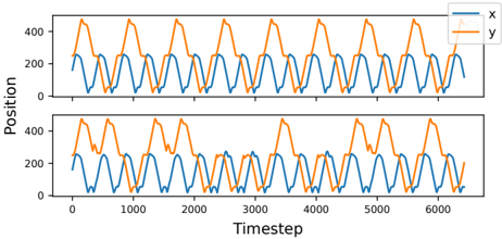
Fig. 8. The coordinates of the agent for 7000 timesteps in the prediction phase. The plots in blue show the x axis coordinates while the ones in red show the y axis coordinates. The figure on top shows the results for the standard 8 sequence [ABABAB..], the figure at the bottom shows the results for a randomly generated sequence [AABAABBBABBAABAB], where 'A' is the left loop and 'B' is the right loop.
<details>
<summary>Image 11 Details</summary>
### Visual Description
## Line Graphs: Position vs. Timestep for Variables x and y
### Overview
The image contains two vertically stacked line graphs, each plotting two variables (x and y) against timesteps. Both graphs share identical axes labels and scales, with timesteps ranging from 0 to 6000 and position values from 0 to 400. The top graph exhibits sharper oscillations, while the bottom graph shows smoother, more damped behavior.
### Components/Axes
- **X-axis**: Labeled "Timestep," with increments at 0, 1000, 2000, 3000, 4000, 5000, and 6000.
- **Y-axis**: Labeled "Position," with increments at 0, 200, and 400.
- **Legend**: Located in the top-right corner of both graphs, with:
- **Blue line**: Represents variable **x**.
- **Orange line**: Represents variable **y**.
- **Graph Structure**: Two identical axes configurations, with the top graph showing more pronounced peaks and the bottom graph displaying attenuated oscillations.
### Detailed Analysis
#### Top Graph
- **x (Blue)**: Peaks reach approximately **400** at timesteps ~500, 1500, 2500, 3500, 4500, and 5500. Troughs dip to ~100 at midpoints between peaks.
- **y (Orange)**: Peaks align with x but are slightly offset, reaching ~350 at timesteps ~1000, 2000, 3000, 4000, and 5000. Troughs remain near ~150.
#### Bottom Graph
- **x (Blue)**: Peaks reduced to ~250 at timesteps ~500, 1500, 2500, 3500, 4500, and 5500. Troughs stabilize near ~120.
- **y (Orange)**: Peaks align with x but are dampened, reaching ~200 at timesteps ~1000, 2000, 3000, 4000, and 5000. A notable dip occurs at ~5000 timesteps, dropping to ~100.
### Key Observations
1. **Top Graph**: Both variables exhibit synchronized oscillations with high amplitude (~400 for x, ~350 for y).
2. **Bottom Graph**: Oscillations are damped, with x and y peaking at ~250 and ~200, respectively. The y variable shows an anomalous dip at ~5000 timesteps.
3. **Phase Relationship**: In both graphs, y lags slightly behind x in peak timing, suggesting a potential causal or reactive relationship.
### Interpretation
The data suggests a time-dependent system where variable x drives oscillations, with y responding in a correlated but slightly delayed manner. The top graph may represent an initial, high-energy state, while the bottom graph reflects a stabilized or damped system. The anomalous dip in y at ~5000 timesteps in the bottom graph could indicate an external perturbation or system failure. These patterns are consistent with oscillatory systems in physics, engineering, or signal processing, where phase shifts and damping are common.
</details>
manipulating prediction of the outcome. Whereas both regions of the anterior cortex and present in mammals, [13] reports that another region, the lateral prefrontal cortex, is unique in primates and has been developed to implement the learning of contextual rules and to possibly act in a hierarchical way in the control of the other regions. We have proposed an elementary implementation of the lateral prefrontal cortex in the second experiment, adding explicit contextual inputs as a basis to form contextual rules. It was accordingly very important to observe that it was then possible to explicitly manipulate the rules and form flexible behavior, whereas in the previous case, rules were implicitly present in the memory but not manipulable.
This simple model shows that the interpretation of the behavior by an observer and the actual behavior might greatly differ even when we can make accurate prediction about the behavior. Such prediction can be incidentally true without actually revealing the true nature of the underlying mechanisms. Based on the reservoir computing framework which can be invoked for both premotor and prefrontal regions, we have implemented models which are structurally similar (as it is the case for that regions) and we have shown that a simple difference related to their inputs can orient then toward implicit or explicit learning as respectively observed in the premotor and lateral prefrontal regions. It will be important in future work to see how these regions are associated to combine both modes of learning and switch from on to the other depending on the complexity of the task.
## REFERENCES
- [1] A. Cleeremans, 'Implicit learning and implicit memory,' Encyclopedia of Consciousness , p. 369-381, 2009. [Online]. Available: http: //dx.doi.org/10.1016/B978-012373873-8.00047-5
- [2] A. Cleeremans, B. Timmermans, and A. Pasquali, 'Consciousness and metarepresentation: A computational sketch,' Neural Networks , vol. 20, no. 9, pp. 1032-1039, 2007.
- [3] B. A. Clegg, G. J. DiGirolamo, and S. W. Keele, 'Sequence learning,' Trends in cognitive sciences , vol. 2, no. 8, pp. 275-281, 1998.
- [4] A. S. Reber, Implicit Learning and Tacit Knowledge . Oxford University Press, Sep 1996. [Online]. Available: http://dx.doi.org/10.1093/acprof: oso/9780195106589.001.0001
- [5] Z. Dienes and D. Berry, 'Implicit learning: Below the subjective threshold,' Psychonomic bulletin & review , vol. 4, no. 1, pp. 3-23, 1997.
- [6] P. Dominey, M. Arbib, and J.-P. Joseph, 'A model of corticostriatal plasticity for learning oculomotor associations and sequences,' Journal of cognitive neuroscience , vol. 7, no. 3, pp. 311-336, 1995.
- [7] J. Tani and S. Nolfi, 'Learning to perceive the world as articulated: an approach for hierarchical learning in sensory-motor systems,' Neural Networks , vol. 12, no. 7-8, pp. 1131-1141, 1999.
- [8] E. Aislan Antonelo and B. Schrauwen, 'On learning navigation behaviors for small mobile robots with reservoir computing architectures,' IEEE Transactions on Neural Networks and Learning Systems , vol. 26, no. 4, p. 763-780, Apr 2015. [Online]. Available: http://dx.doi.org/10.1109/TNNLS.2014.2323247
- [9] E. Antonelo and B. Schrauwen, 'Learning slow features with reservoir computing for biologically-inspired robot localization,' Neural Networks , vol. 25, p. 178-190, Jan 2012. [Online]. Available: http://dx.doi.org/10.1016/j.neunet.2011.08.004
- [10] L. M. Frank, E. N. Brown, and M. Wilson, 'Trajectory encoding in the hippocampus and entorhinal cortex,' Neuron , vol. 27, no. 1, pp. 169178, 2000.
- [11] N. Trouvain, L. Pedrelli, T. T. Dinh, and X. Hinaut, 'ReservoirPy: An efficient and user-friendly library to design echo state networks,' in Artificial Neural Networks and Machine Learning -ICANN 2020 . Springer International Publishing, 2020, pp. 494-505. [Online]. Available: https://doi.org/10.1007/978-3-030-61616-8 40
- [12] J. Bergstra, B. Komer, C. Eliasmith, D. Yamins, and D. D. Cox, 'Hyperopt: a python library for model selection and hyperparameter optimization,' Computational Science & Discovery , vol. 8, no. 1, p. 014008, 2015.
- [13] E. Koechlin, 'An evolutionary computational theory of prefrontal executive function in decision-making.' Philosophical transactions of the Royal Society of London. Series B, Biological sciences , vol. 369, no. 1655, pp. 20 130 474+, Nov. 2014. [Online]. Available: http://dx.doi.org/10.1098/rstb.2013.0474