# Deep Multi-Frame MVDR Filtering for Binaural Noise Reduction
**Authors**: Marvin Tammen, Simon Doclo
## DEEPMULTI-FRAMEMVDRFILTERINGFORBINAURALNOISEREDUCTION
Marvin Tammen, Simon Doclo
Department of Medical Physics and Acoustics and Cluster of Excellence Hearing4all University of Oldenburg, Germany { marvin.tammen, simon.doclo } @uni-oldenburg.de
## ABSTRACT
To improve speech intelligibility and speech quality in noisy environments, binaural noise reduction algorithms for head-mounted assistive listening devices are of crucial importance. Several binaural noise reduction algorithms such as the well-known binaural minimum variance distortionless response (MVDR) beamformer have been proposed, which exploit spatial correlations of both the target speech and the noise components. Furthermore, for singlemicrophone scenarios, multi-frame algorithms such as the multiframe MVDR (MFMVDR) filter have been proposed, which exploit temporal instead of spatial correlations. In this contribution, we propose a binaural extension of the MFMVDR filter, which exploits both spatial and temporal correlations. The binaural MFMVDR filters are embedded in an end-to-end deep learning framework, where the required parameters, i.e., the speech spatio-temporal correlation vectors as well as the (inverse) noise spatio-temporal covariance matrix, are estimated by temporal convolutional networks (TCNs) that are trained by minimizing the mean spectral absolute error loss function. Simulation results comprising measured binaural room impulses and diverse noise sources at signal-to-noise ratios from -5 dB to 20 dB demonstrate the advantage of utilizing the binaural MFMVDR filter structure over directly estimating the binaural multi-frame filter coefficients with TCNs.
Index Terms -binaural noise reduction, multi-frame filtering, supervised learning
## 1. INTRODUCTION
In many speech communication scenarios, head-mounted assistive listening devices such as binaural hearing aids capture not only the target speaker, but also ambient noise, resulting in a degradation of speech quality and speech intelligibility. Hence, several binaural noise reduction algorithms have been proposed, which typically assume that adjacent short-time Fourier transform (STFT) coefficients are uncorrelated over time. This assumption is suitable when considering sufficiently long frames and a small frame overlap. In that case, the speech STFT coefficients at a left and right reference microphone can be estimated by applying (complex-valued) single-frame binaural filters to the available microphone signals. Several approaches have been proposed to estimate these single-frame binaural filters, which can be categorized into statistical model-based approaches (e.g., [1][4]) and supervised learning-based approaches (e.g., [5]-[11]). While the statistical model-based approaches can be mainly differentiated w.r.t. their underlying optimization problem and how the required
This work was funded by the Deutsche Forschungsgemeinschaft (DFG,
German Research Foundation) under Germany's Excellence Strategy - EXC 2177/1 - Project ID 390895286.
parameters are estimated, the supervised learning-based approaches mainly differ in the used deep neural network (DNN) architecture and loss function.
With the goal of exploiting temporal correlations between neighboring STFT coefficients, multi-frame methods have been proposed for both single- and multi-microphone noise reduction, which apply (complex-valued) multi-frame filters to the most recent noisy STFT coefficients of each microphone. Similarly to the single-frame methods mentioned above, several approaches have been proposed to estimate these multi-frame filters, which can again be categorized into statistical model-based approaches (e.g., [12], [13]) and supervised learning-based approaches (e.g., [14]-[18]). In contrast to the singleframe approaches, however, there is a lack of studies that considered multi-frame approaches for binaural noise reduction.
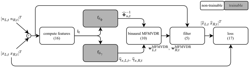
Aiming at utilizing both spatial correlations as in the binaural minimum variance distortionless response (MVDR) beamformer [1], [3] and temporal correlations as in the multi-frame MVDR (MFMVDR) filter [12], [16], we propose to extend the MFMVDR filter to binaural listening scenarios. To implement the binaural MFMVDR filter, estimates of the speech spatio-temporal correlation vectors (STCVs) as well as the (inverse) noise spatio-temporal covariance matrix (STCM) are required. Similarly as in [16], the binaural MFMVDR filter is embedded in an end-to-end supervised learning framework as shown in Fig. 1, where all required parameters are estimated using temporal convolutional networks (TCNs) that are trained using the mean spectral absolute error (MSAE) loss function [19]. Simulation results using measured binaural room impulse responses from [20] as well as clean speech and noise from the third Deep Noise Suppression Challenge (DNS3) [21] at signal-to-noiseratios (SNRs) from -5dB to 20dB show that the proposed deep binaural MFMVDR filter outperforms directly estimating the singleor multi-frame binaural filter coefficients using TCNs, i.e., without exploiting the structure of the deep binaural MFMVDR filter.
## 2. SIGNALMODEL
We consider an acoustic scenario with a single speech source and a single noise source, both located in a reverberant room, recorded by binaural hearing aids with M microphones. In the STFT domain, the noisy microphone signals y m,f,t are given by
<!-- formula-not-decoded -->
where x m,f,t and n m,f,t denote the speech and noise components, respectively, at the m -th microphone, the f -th frequency bin, and the t -th time frame. Since all frequency bins are processed independently, the index f will be omitted in the remainder of this paper.
In single -microphonemulti-framenoisereductionalgorithms[12],
Fig. 1 . Block diagram of the proposed deep binaural MFMVDR filter.
<details>
<summary>Image 1 Details</summary>
### Visual Description
\n
## Diagram: Binaural MFMVDR Processing Flow
### Overview
The image depicts a block diagram illustrating a binaural Multi-Frequency Multi-Channel Wiener Filter (MFMVDR) processing pipeline. The diagram shows the flow of data through several stages, including feature computation, binaural MFMVDR processing, filtering, and loss calculation. The diagram also indicates which components are trainable and non-trainable.
### Components/Axes
The diagram consists of the following components:
* **Input:** `(nL,t, rL,t)ᵀ` and `(xL,t, xR,t)ᵀ`
* **Compute Features:** (16)
* **Feature Vector:** `iₜ`
* **θθ:** Two grey boxes representing parameters, one labeled `Φₙ,ₜ⁻¹` and the other `θₜ`.
* **Binaural MFMVDR:** (10) with outputs `wL,tMFMVDR` and `wR,tMFMVDR`
* **Filter:** (5)
* **Loss:** (17)
* **Output:** `(n̂L,t, n̂R,t)ᵀ`
* **Legend:**
* White box with black text: "non-trainable"
* Black box with white text: "trainable"
### Detailed Analysis or Content Details
The diagram shows the following data flow:
1. **Input:** Two input vectors, `(nL,t, rL,t)ᵀ` and `(xL,t, xR,t)ᵀ`, are summed at a summation junction (represented by a circle with a plus sign).
2. **Compute Features:** The summed input is fed into a "compute features" block, which outputs a feature vector `iₜ`. This block contains the number (16) indicating the number of features.
3. **Binaural MFMVDR:** The feature vector `iₜ` is input to two parameter blocks `θₜ` and `Φₙ,ₜ⁻¹`. The outputs of these blocks, along with `iₜ`, are fed into a "binaural MFMVDR" block, which outputs two weight vectors: `wL,tMFMVDR` and `wR,tMFMVDR`. This block contains the number (10) indicating the number of parameters.
4. **Filter:** The weight vectors `wL,tMFMVDR` and `wR,tMFMVDR` are fed into a "filter" block, which outputs a filtered vector. This block contains the number (5) indicating the number of parameters.
5. **Loss:** The output of the filter is compared to the original input `(n̂L,t, n̂R,t)ᵀ` in a "loss" block, which calculates a loss value. This block contains the number (17) indicating the number of parameters.
6. **Feedback Loop:** The output of the "loss" block is fed back into the parameter blocks `θₜ` and `Φₙ,ₜ⁻¹`, indicating a training or optimization process.
The diagram also indicates the trainability of each block:
* The blocks `θₜ` and `Φₙ,ₜ⁻¹` are marked as "non-trainable" (white box with black text).
* The blocks "compute features", "binaural MFMVDR", "filter", and "loss" are marked as "trainable" (black box with white text).
### Key Observations
The diagram highlights a closed-loop system where the loss is used to update the trainable parameters. The separation of trainable and non-trainable components suggests a hybrid approach to parameter estimation. The numbers in parentheses likely represent the number of parameters or dimensions within each block.
### Interpretation
This diagram represents a signal processing pipeline for binaural audio, likely for tasks such as noise reduction or source separation. The MFMVDR filter is a key component, and the diagram illustrates how it is integrated into a larger trainable system. The feedback loop indicates that the system is designed to learn and adapt its parameters to minimize the loss function, improving its performance over time. The distinction between trainable and non-trainable parameters suggests that some aspects of the system are fixed, while others are learned from data. The diagram provides a high-level overview of the system architecture and data flow, without specifying the exact mathematical details of each block. The numbers in parentheses likely represent the dimensionality or number of parameters within each block, providing a sense of the complexity of each component. The diagram is a conceptual representation of the system, and the actual implementation may involve additional details and optimizations.
</details>
[16], the noisy multi-frame vector ¯ y m,t ∈ C N is defined as
<!-- formula-not-decoded -->
with ◦ T denoting the transpose operator, such that (1) can be written as ¯ y m,t =¯ x m,t +¯ n m,t . In this case, using a complex-valued multiframe filter ¯ w m,t ∈ C N , the speech component x m,t is estimated as
<!-- formula-not-decoded -->
where ◦ H denotes the conjugate transpose operator.
In multi -microphonemulti-framenoisereductionalgorithms[13], [17], [18], the noisy multi-microphone multi-frame vector y m,t ∈ C NM is defined as
<!-- formula-not-decoded -->
such that (1) can be written as y t = x t + n t . Without loss of generality, in this paper we consider the case M =2 , with one hearing aid per side and one microphone per hearing aid, i.e., m ∈{ L,R } , where L and R denote the left and right side, respectively. In this case, using (complex-valued) binaural multi-frame filters w m,t ∈ C 2 N with 2 N taps each, the binaural speech components are estimated as
<!-- formula-not-decoded -->
Assumingthatthespeechandnoisecomponentsarespatio-temporally uncorrelated, the noisy spatio-temporal covariance matrix (STCM) Φ y,t = E{ y t y H t } ∈ C 2 N × 2 N , with E{◦} the expectation operator, can be written as
<!-- formula-not-decoded -->
where Φ x,t and Φ n,t are defined similarly as Φ y,t .
In order to exploit speech correlations across successive time frames, it has been proposed in [12] to decompose the (singlemicrophone) multi-frame speech vector into a temporally correlated and a temporally uncorrelated component. Similarly, the binaural multi-frame speech vector x t can be decomposed into a spatiotemporally correlated and a spatio-temporally uncorrelated component w.r.t. the current left or the right speech STFT coefficient x m,t :
<!-- formula-not-decoded -->
The highly time-varying left or right speech spatio-temporal correlation vector (STCV) γ x,m,t ∈ C 2 N describes the correlation between the N most recent left and right speech STFT coefficients and the current left or the right speech STFT coefficient x m,t , and it is defined as
<!-- formula-not-decoded -->
where ◦ ∗ denotes the conjugate operator and with e T L γ x,L,t = e T R γ x,R,t = 1 . Here, e L and e R denote selection vectors with their first or N +1 -th element equal to 1 , respectively, and the other elements equal to 0 .
## 3. DEEPBINAURALMULTI-FRAMEMVDRFILTER
Aiming at minimizing the output noise power spectral density while leaving the correlated speech component undistorted, in [12] the MFMVDR filter for single-microphone noise reduction has been proposed. In this paper, we propose to extend the single-microphone MFMVDR filter to binaural scenarios by considering the spatiotemporal correlations of the speech and noise components for the left and right side, i.e.,
<!-- formula-not-decoded -->
Solving this optimization problem, the binaural MFMVDR filters are given by
<!-- formula-not-decoded -->
As has been shown for the single-microphone MFMVDRfilter [22], the performance of the (binaural) MFMVDR filter depends on how well the required parameters, i.e., the inverse noise STCM as well as the speech STCVs, are estimated from the noisy STFT coefficients. In contrast to using statistical model-based estimators similar to [23], we embed the binaural MFMVDR filter in an end-to-end supervised learning framework similar to [16], with the parameters estimated by TCNs (see Fig. 1). The TCNs are trained by minimizing the MSAEloss function [19] computed at the output of the deep binaural MFMVDR filter instead of providing explicit parameter labels. Apriori knowledge about the properties of the estimated parameters is exploited as described in the following two sections.
## 3.1. Speech Spatio-Temporal Correlation Vector
The left and right speech STCVs each are two 2 N -dimensional complex-valued vectors (cf. (8)), hence consisting of 8 N real -valued coefficients h R γ,t ∈ R 8 N ( 4 N for the real part and 4 N for the imaginary part). To estimate these real-valued coefficients, we propose to use a TCN f θ γ with parameters θ γ , which is fed input features i t derived from the noisy STFT coefficients, i.e.,
<!-- formula-not-decoded -->
with the features i t defined in (16). To construct a 4 N -dimensional complex-valued vector ̂ h C γ,t from the 8 N -dimensional real-valued vector ̂ h R γ,t , the first 4 N elements of ̂ h R γ,t are used for the real components and the second 4 N elements are used for the imaginary components, i.e.,
<!-- formula-not-decoded -->
where j 2 = -1 . To ensure that the first or N +1 -th element of the speech STCVs is equal to 1 (cf. (8)), the speech STCVs are finally obtained as
<!-- formula-not-decoded -->
## 3.2. Spatio-Temporal Covariance Matrices
Since the 2 N × 2 N -dimensional STCM Φ n,t can be assumed to be Hermitian positive-definite, also its inverse Φ -1 n,t as required in (10) can be assumed to be Hermitian positive-definite. Hence, Φ -1 n,t has a unique Cholesky decomposition [24]:
<!-- formula-not-decoded -->
with L t ∈ C 2 N × 2 N a lower triangular matrix with positive real-valued diagonal. Due to its structure, L is determined by (2 N ) 2 real-valued coefficients. Similarly to the procedure for estimating the speech STCVs,weuseaTCN f θ Φ with parameters θ Φ , which is fed input features i t , to estimate these real-valued coefficients ̂ h R Φ ,t ∈ R (2 N ) 2 , i.e.,
<!-- formula-not-decoded -->
Using ̂ h R Φ ,t , the lower triangular matrix with positive real-valued diagonal ̂ L t is assembled. Finally, an estimate of Φ -1 n,t is obtained using (14) by replacing L t with its estimate ̂ L t .
## 4. SIMULATIONS
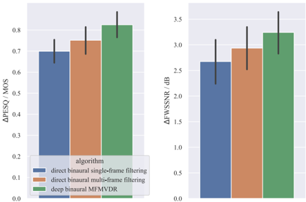
In this section, the binaural noise reduction performance of the proposed deep binaural MFMVDR filter is compared with a number of baseline algorithms, which are described in Section 4.1. Sections 4.2 and 4.3 deal with the used datasets and the simulation settings, respectively. In Section 4.4, the simulation results are presented in terms of the perceptual evaluation of speech quality (PESQ) [25] and frequency-weighted segmental SNR (FWSSNR) [26] improvement.
## 4.1. Baseline Algorithms
The following baseline algorithms have been considered to allow investigating the effect of not using vs. using the proposed deep binaural MFMVDR structure for binaural multi-frame filtering. To achieve this goal, for the baseline algorithms the binaural multi-frame filters in (5) are not obtained using the binaural MFMVDR structure. Instead, the real and imaginary components of the baseline binaural multi-frame filters are directly estimated by a TCN, i.e., without the intermediate steps of speech STCVs and inverse noise STCM estimation and computation of (10). In addition, we investigate the effect of binaural single-frame vs. binaural multi-frame filtering. More specifically, we use the following end-to-end supervised learning-based baseline algorithms:
direct binaural single-frame filtering With N =1 and w B1 m,t ∈ C 2 , only spatial filtering is performed. The filter coefficients are estimated using a TCN f B1 with parameters θ B1 , i.e., w B1 m,t = f B1 { i t } . The real and imaginary parts of the filter coefficients w B1 m,t are bounded to [ -1 , 1] using a hyperbolic tangent activation function.
direct binaural multi-frame filtering With N = 3 and w B2 m,t ∈ C 2 N , both spatial and temporal filtering are performed. The filter coefficients are estimated using a TCN f B2 with parameters θ B2 , i.e., w B2 m,t = f B2 { i t } . The real and imaginary parts of the filter coefficients w B2 m,t are bounded to [ -1 , 1] using a hyperbolic tangent activation function. These bounds are motivated by [14].
## 4.2. Dataset
To train and validate the considered algorithms, we used simulated binaural room impulse responses (BRIRs) from the training subset of the first Clarity Enhancement Challenge (CEC1) dataset [27] as well as clean speech (English read book sentences) and noise from the training subset of the third Deep Noise Suppression Challenge (DNS3) dataset [21]. These BRIRs were simulated by considering a randomly positioned directed speech source and an omnidirectional noise point source captured by binaural behind-the-ear hearing aids in randomly sized rooms with 'low to moderate' reverberation, i.e., around 0 . 2s to 0 . 4s . The speech source was always located at an angle within ± 30 ° w.r.t. the listener, while the noise source could be positioned everywhere in the room except for less than 1m from the walls or the listener. Surface absorption coefficients were varied to simulate various room characteristics such as doors, windows, curtains, rugs, or furniture. In total, 6000 room configurations were considered. Clean speech and noise were convolved with their corresponding BRIRs before being mixed at better ear SNRs from 0dB to 15dB . In total, the training and validation datasets have a length of 80h and 20h , respectively.
To evaluate the considered algorithms, we used measured BRIRs from the dataset proposed in [20] as well as clean speech and noise from the official test subset of the deep noise suppression (DNS) dataset [28]. The dataset in [20] comprises BRIRs measured with binaural behind-the-ear hearing aids 'for multiple, realistic head and sound-source positions in four natural environments reflecting dailylife communication situations with different reverberation times'. The configuration of these hearing aids matches the configuration considered in the training and validation datasets. Clean speech and noise were convolved with the BRIRs before being mixed at better ear SNRs from -5dB to 20dB . In total, 100 utterances, each of length 10s , were considered in the evaluation. Note that, especially due to the use of simulated vs. measured BRIRs, there is considerable mismatch between the training and validation datasets on the one hand and the evaluation dataset on the other hand. All datasets were used at a sampling frequency of 16kHz .
## 4.3. Settings
For the STFT used in all considered algorithms, √ Hann windows with a frame length of 8ms and a frame shift of 2ms were used for both analysis and synthesis. As input features, we used a concatenation of the logarithmic magnitude, the cosine of the phase, and the sine of the phase, of the noisy left and right STFT coefficients, i.e.,
<!-- formula-not-decoded -->
where ◦ denotes the phase of ◦ . Note that both the cosine and sine of the noisy phase are chosen to prevent an ambiguous phase representation.
The multi-frame algorithms use N = 5 frames, resulting in the capability of exploiting temporal correlations within 16ms . To decrease distortion of the speech and residual noise components, a minimum gain of -20dB was included in all algorithms.
ToestimatetherequiredparametersofthedeepbinauralMFMVDR filter or the filter coefficients of the baseline algorithms, we used TCNs, with their hyperparameters fixed to 2 stacks of 6 layers, yielding a temporal receptive field size of 512ms . Since the deep binaural MFMVDRfilter uses two TCNs and the number of real-valued coefficients differs per considered algorithm, the hidden dimension size of the TCNs was varied per algorithm to result in similar numbers of trainable weights for all algorithms, i.e., 6 . 2 × 10 6 . While also the other hyperparameters could have been varied to this end, only varying the hidden dimension size results in TCNs with the same temporal receptive field size, which is required for a fair comparison. To prevent division by 0 , a small constant was added to the denominator in (13).
Asloss function, the MSAE proposed in [19] was used, where the loss was averaged across the batch, the left and right output signals, and the frequency bins and time frames, i.e.,
<!-- formula-not-decoded -->
where B denotes the batch size, F and T denote the numbers of frequency bins and time frames in an utterance, and β =0 . 4 [19].
The TCNs were implemented based on the official Conv-TasNet implementation 1 , and they were trained for a maximum of 150 epochs with early stopping using the AdamW optimizer [29]. The learning rate was initialized as 3 × 10 -4 , and it was halved after 3 epochs without an improvement on the validation dataset. Gradient 2 -norms were clipped to 5 , and the batch size was 8 .
The simulations were implemented using PyTorch 1.10 [30] and performed on NVIDIA GeForce®RTX A5000 graphics cards. A PyTorch implementation of the compared algorithms as well as the model weights used in the evaluation will be made publicly available upon publication.
## 4.4. Results
For all considered algorithms, Fig. 2 depicts the improvement in terms of PESQ and FWSSNR w.r.t. the noisy microphone signals on the evaluation dataset. Note that, similarly as for the MSAE loss function in (17), PESQ and FWSSNR improvements are simply averaged across the left and right output signals [10].
First, a considerable improvement in terms of PESQ and FWSSNR can be observed for all algorithms, with the deep binaural MFMVDR filter outperforming the baseline algorithms. Second, comparing the baseline algorithms, it can be observed that increasing the degrees of freedom of the filter, i.e., by allowing for a binaural multi-frame vs. a binaural single-frame filter, improves binaural noise reduction performance. Third, by enforcing the binaural MFMVDR structure on the binaural multi-frame filter, binaural noise reduction performance is further increased.
1 https://github.com/naplab/Conv-TasNet
Fig. 2 . Mean and standard deviation of the PESQ and FWSSNR improvementsobtainedontheevaluationdataset. ThemeannoisyPESQ score is 1 . 74MOS and the mean noisy FWSSNR score is 14 . 08dB .
<details>
<summary>Image 2 Details</summary>
### Visual Description
\n
## Bar Chart: Performance Comparison of Binaural Filtering Algorithms
### Overview
This image presents a comparative analysis of three binaural filtering algorithms using two different metrics: ΔPESQ / MOS (left chart) and ΔFWSSNR / dB (right chart). The algorithms are: direct binaural single-frame filtering, direct binaural multi-frame filtering, and deep binaural MFMVDR. Each bar represents the mean performance of an algorithm, with error bars indicating the variability.
### Components/Axes
* **X-axis (Both Charts):** "algorithm" with categories: "direct binaural single-frame filtering", "direct binaural multi-frame filtering", and "deep binaural MFMVDR".
* **Y-axis (Left Chart):** "ΔPESQ / MOS". Scale ranges from 0.0 to 0.9, with increments of 0.1.
* **Y-axis (Right Chart):** "ΔFWSSNR / dB". Scale ranges from 0.0 to 3.5, with increments of 0.5.
* **Legend (Bottom-Left):**
* Blue: "direct binaural single-frame filtering"
* Orange: "direct binaural multi-frame filtering"
* Green: "deep binaural MFMVDR"
### Detailed Analysis or Content Details
**Left Chart (ΔPESQ / MOS):**
* **Direct Binaural Single-Frame Filtering (Blue):** The bar is approximately 0.72 ± 0.08. The bar rises to approximately 0.72, with the top of the error bar reaching around 0.80 and the bottom around 0.64.
* **Direct Binaural Multi-Frame Filtering (Orange):** The bar is approximately 0.75 ± 0.07. The bar rises to approximately 0.75, with the top of the error bar reaching around 0.82 and the bottom around 0.68.
* **Deep Binaural MFMVDR (Green):** The bar is approximately 0.83 ± 0.06. The bar rises to approximately 0.83, with the top of the error bar reaching around 0.89 and the bottom around 0.77.
**Right Chart (ΔFWSSNR / dB):**
* **Direct Binaural Single-Frame Filtering (Blue):** The bar is approximately 2.6 ± 0.5. The bar rises to approximately 2.6, with the top of the error bar reaching around 3.1 and the bottom around 2.1.
* **Direct Binaural Multi-Frame Filtering (Orange):** The bar is approximately 3.0 ± 0.4. The bar rises to approximately 3.0, with the top of the error bar reaching around 3.4 and the bottom around 2.6.
* **Deep Binaural MFMVDR (Green):** The bar is approximately 3.2 ± 0.5. The bar rises to approximately 3.2, with the top of the error bar reaching around 3.7 and the bottom around 2.7.
### Key Observations
* In both charts, the "deep binaural MFMVDR" algorithm consistently demonstrates the highest mean performance.
* The "direct binaural multi-frame filtering" algorithm outperforms the "direct binaural single-frame filtering" algorithm in both metrics.
* The error bars indicate that the variability in performance is relatively similar across all algorithms for both metrics.
* The PESQ metric shows smaller differences between algorithms than the FWSSNR metric.
### Interpretation
The data suggests that the "deep binaural MFMVDR" algorithm provides the best performance in terms of both perceptual quality (ΔPESQ / MOS) and signal-to-noise ratio (ΔFWSSNR / dB) compared to the direct filtering methods. The improvement from single-frame to multi-frame filtering indicates that incorporating temporal information enhances performance. The larger differences observed in the FWSSNR metric suggest that the deep learning approach has a more significant impact on reducing noise and improving signal clarity than on directly improving perceived audio quality. The error bars suggest that the observed differences are statistically meaningful, but there is still some variability in the results. This could be due to variations in the input data or the specific implementation of the algorithms. The charts provide a clear quantitative comparison of the effectiveness of different binaural filtering techniques.
</details>
Audio examples for the compared algorithms are available online 2 .
## 5. CONCLUSION
In this paper we proposed a binaural extension of the MFMVDR filter, which is capable of utilizing both spatial and temporal correlations of the speech and noise components. To estimate the speech STCVs as well as the inverse noise STCM required by the binaural MFMVDR filter, we use TCNs, which are trained by embedding the binaural MFMVDR filter in an end-to-end supervised learning framework and minimizing the MSAE loss function. Simulations comprising measured binaural room impulse responses as well as diverse noise sources at SNRs in -5dB to 20dB demonstrate the advantage of binaural multi-frame filtering over binaural single-frame filtering as well as employing the binaural MFMVDR structure over directly estimating the single- or multi-frame binaural filters using TCNs.
## References
- [1] S. Doclo, W. Kellermann, S. Makino, et al. , 'Multichannel Signal Enhancement Algorithms for Assisted Listening Devices: Exploiting spatial diversity using multiple microphones,' IEEE Signal Processing Magazine , vol. 32, no. 2, pp. 18-30, Mar. 2015.
- [2] E. Hadad, S. Doclo, and S. Gannot, 'The Binaural LCMV Beamformer and its Performance Analysis,' IEEE/ACM Transactions on Audio, Speech, and Language Processing , vol. 24, no. 3, pp. 543-558, Mar. 2016.
- [3] S. Gannot, E. Vincent, S. Markovich-Golan, et al. , 'A Consolidated Perspective on Multimicrophone Speech Enhancement and Source Separation,' IEEE/ACM Transactions on Audio, Speech, and Language Processing , vol. 25, no. 4, pp. 692730, Jan. 2017.
- [4] S. Doclo, S. Gannot, D. Marquardt, et al. , 'Binaural Speech Processing with Application to Hearing Devices,' in Audio
2 https://uol.de/en/sigproc/research/audio-demos/ binaural-noise-reduction/deep-bmfmvdr
- Source Separation and Speech Enhancement , John Wiley & Sons, Ltd, Aug. 2018, pp. 413-442.
- [5] A. H. Moore, L. Lightburn, W. Xue, et al. , 'Binaural MaskInformed Speech Enhancement for Hearing AIDS with Head Tracking,' in Proc. 16th International Workshop on Acoustic Signal Enhancement (IWAENC) , Tokyo, Japan, Sep. 2018, pp. 461-465.
- [6] X. Sun, R. Xia, J. Li, et al. , 'A Deep Learning Based Binaural Speech Enhancement Approach with Spatial Cues Preservation,' in Proc. IEEE International Conference on Acoustics, Speech and Signal Processing (ICASSP) , Brighton, UK, May 2019.
- [7] C. Han, Y. Luo, and N. Mesgarani, 'Real-Time Binaural Speech Separation with Preserved Spatial Cues,' in Proc. IEEE International Conference on Acoustics, Speech and Signal Processing (ICASSP) , Barcelona, Spain, May 2020, pp. 6404-6408.
- [8] Z. Sun, Y. Li, H. Jiang, et al. , 'A Supervised Speech Enhancement Method for Smartphone-Based Binaural Hearing Aids,' IEEE Transactions on Biomedical Circuits and Systems , vol. 14, no. 5, pp. 951-960, Oct. 2020.
- [9] J.-H. Kim, J. Choi, J. Son, et al. , 'MIMO Noise Suppression Preserving Spatial Cues for Sound Source Localization in Mobile Robot,' in Proc. IEEE International Symposium on Circuits and Systems (ISCAS) , Daegu, Korea, May 2021.
- [10] B. J. Borgstr¨ om, M. S. Brandstein, G. A. Ciccarelli, et al. , 'Speaker separation in realistic noise environments with applications to a cognitively-controlled hearing aid,' Neural Networks , pp. 136-147, Mar. 2021.
- [11] T. Green, G. Hilkhuysen, M. Huckvale, et al. , 'Speech recognition with a hearing-aid processing scheme combining beamforming with mask-informed speech enhancement,' Trends in Hearing , vol. 26, Jan. 2022.
- [12] Y. A. Huang and J. Benesty, 'A Multi-Frame Approach to the Frequency-Domain Single-Channel Noise Reduction Problem,' IEEE Trans. Audio, Speech, and Language Processing , vol. 20, no. 4, pp. 1256-1269, May 2012.
- [13] E. A. P. Habets, J. Benesty, and J. Chen, 'Multi-microphone noise reduction using interchannel and interframe correlations,' in Proc. IEEE International Conference on Acoustics, Speech and Signal Processing (ICASSP) , Kyoto, Japan, Mar. 2012, pp. 305-308.
- [14] W. Mack and E. A. P. Habets, 'Deep Filtering: Signal Extraction and Reconstruction Using Complex Time-Frequency Filters,' IEEE Signal Processing Letters , vol. 27, pp. 61-65, 2020.
- [15] A.Aroudi,M.Delcroix,T.Nakatani, et al. , 'Cognitive-Driven Convolutional Beamforming Using EEG-Based Auditory Attention Decoding,' in Proc. IEEE 30th International Workshop on Machine Learning for Signal Processing (MLSP) , Espoo, Finland, Sep. 2020.
- [16] M. Tammen and S. Doclo, 'Deep Multi-Frame MVDR Filtering for Single-Microphone Speech Enhancement,' in Proc. IEEE International Conference on Acoustics, Speech and Signal Processing (ICASSP) , Toronto, Ontario, Canada, Jun. 2021, pp. 8443-8447.
- [17] Z. Zhang, Y. Xu, M. Yu, et al. , 'Multi-Channel Multi-Frame ADL-MVDR for Target Speech Separation,' IEEE/ACM Trans. Audio, Speech, and Language Processing , vol. 29, pp. 3526-3540, Nov. 2021.
- [18] Z.-Q. Wang, H. Erdogan, S. Wisdom, et al. , 'Sequential Multi-Frame Neural Beamforming for Speech Separation and Enhancement,' in Proc. IEEE Spoken Language Technology Workshop (SLT) , Shenzhen, China, Jan. 2021, pp. 905-911.
- [19] Z.-Q. Wang, P. Wang, and D. Wang, 'Complex Spectral Mapping for Single- and Multi-Channel Speech Enhancement and Robust ASR,' IEEE/ACM Trans. Audio, Speech, and Language Processing , vol. 28, pp. 1778-1787, May 2020.
- [20] H.Kayser,S.D.Ewert,J.Anemuller, et al. , 'Database of Multichannel In-Ear and Behind-the-Ear Head-Related and Binaural Room Impulse Responses,' EURASIP Journal on Advances in Signal Processing , vol. 2009, no. 1, Jun. 2009.
- [21] C. K. Reddy, H. Dubey, K. Koishida, et al. , 'INTERSPEECH 2021 Deep Noise Suppression Challenge,' in Proc. Interspeech , Brno, Czech Republic, Aug. 2021, pp. 2796-2800.
- [22] D. Fischer and S. Doclo, 'Sensitivity analysis of the multiframe MVDR filter for single-microphone speech enhancement,' in Proc. European Signal Processing Conference (EUSIPCO) , Kos, Greece, Aug. 2017, pp. 603-607.
- [23] A. Schasse and R. Martin, 'Estimation of Subband Speech Correlations for Noise Reduction via MVDR Processing,' IEEE/ACM Transactions on Audio, Speech, and Language Processing , vol. 22, no. 9, pp. 1355-1365, Sep. 2014.
- [24] A.-L. Cholesky, 'Note sur une m´ ethode de resolution des ´ equations normales provenant de l'application de la m´ ethode des moindres carr´ es ` a un syst` eme d'´ equations lineaires en nombreinferieure ` a celui des inconnues,' Bulletin G´ eod´ esique , vol. 2, no. 1, pp. 67-77, Apr. 1924.
- [25] A. W. Rix, J. G. Beerends, M. P. Hollier, et al. , 'Perceptual evaluation of speech quality (PESQ)-a new method for speech quality assessment of telephone networks and codecs,' in Proc. IEEE International Conference on Acoustics, Speech, and Signal Processing (ICASSP) , Salt Lake City, Utah, USA, May2001, pp. 749-752.
- [26] Y. Hu and P. C. Loizou, 'Evaluation of Objective Quality Measures for Speech Enhancement,' IEEETransactions on Audio, Speech,andLanguageProcessing , vol. 16, no. 1, pp. 229-238, Jan. 2008.
- [27] S. Graetzer, J. Barker, T. J. Cox, et al. , 'Clarity-2021 Challenges: Machine Learning Challenges for Advancing Hearing Aid Processing,' in Proc. Interspeech , Brno, Czech Republic, Aug. 2021, pp. 686-690.
- [28] C. K. Reddy, V. Gopal, R. Cutler, et al. , 'The INTERSPEECH 2020 Deep Noise Suppression Challenge: Datasets, Subjective Testing Framework, and Challenge Results,' in Proc. Interspeech , Shanghai, China, Oct. 2020, pp. 2492-2496.
- [29] I. Loshchilov and F. Hutter, 'Decoupled Weight Decay Regularization,' in Proc. International Conference on Learning Representations (ICLR) , New Orleans, LA, USA, May 2019.
- [30] A. Paszke, S. Gross, F. Massa, et al. , 'Pytorch: An imperative style, high-performance deep learning library,' Advances in neural information processing systems , vol. 32, Dec. 2019.