# Matryoshka Representation Learning
> Equal contribution – AK led the project with extensive support from GB and AR for experimentation.
Abstract
Learned representations are a central component in modern ML systems, serving a multitude of downstream tasks. When training such representations, it is often the case that computational and statistical constraints for each downstream task are unknown. In this context, rigid fixed-capacity representations can be either over or under-accommodating to the task at hand. This leads us to ask: can we design a flexible representation that can adapt to multiple downstream tasks with varying computational resources? Our main contribution is
<details>
<summary>x1.png Details</summary>

### Visual Description
Icon/Small Image (28x28)
</details>
${\rm Matryoshka~Representation~Learning}$ ( ${\rm MRL}$ ) which encodes information at different granularities and allows a single embedding to adapt to the computational constraints of downstream tasks. ${\rm MRL}$ minimally modifies existing representation learning pipelines and imposes no additional cost during inference and deployment. ${\rm MRL}$ learns coarse-to-fine representations that are at least as accurate and rich as independently trained low-dimensional representations. The flexibility within the learned ${\rm Matryoshka~Representations}$ offer: (a) up to $\mathbf{14}×$ smaller embedding size for ImageNet-1K classification at the same level of accuracy; (b) up to $\mathbf{14}×$ real-world speed-ups for large-scale retrieval on ImageNet-1K and 4K; and (c) up to $\mathbf{2}$ % accuracy improvements for long-tail few-shot classification, all while being as robust as the original representations. Finally, we show that ${\rm MRL}$ extends seamlessly to web-scale datasets (ImageNet, JFT) across various modalities – vision (ViT, ResNet), vision + language (ALIGN) and language (BERT). ${\rm MRL}$ code and pretrained models are open-sourced at https://github.com/RAIVNLab/MRL.
1 Introduction
Learned representations [57] are fundamental building blocks of real-world ML systems [66, 91]. Trained once and frozen, $d$ -dimensional representations encode rich information and can be used to perform multiple downstream tasks [4]. The deployment of deep representations has two steps: (1) an expensive yet constant-cost forward pass to compute the representation [29] and (2) utilization of the representation for downstream applications [50, 89]. Compute costs for the latter part of the pipeline scale with the embedding dimensionality as well as the data size ( $N$ ) and label space ( $L$ ). At web-scale [15, 85] this utilization cost overshadows the feature computation cost. The rigidity in these representations forces the use of high-dimensional embedding vectors across multiple tasks despite the varying resource and accuracy constraints that require flexibility.
Human perception of the natural world has a naturally coarse-to-fine granularity [28, 32]. However, perhaps due to the inductive bias of gradient-based training [84], deep learning models tend to diffuse “information” across the entire representation vector. The desired elasticity is usually enabled in the existing flat and fixed representations either through training multiple low-dimensional models [29], jointly optimizing sub-networks of varying capacity [9, 100] or post-hoc compression [38, 60]. Each of these techniques struggle to meet the requirements for adaptive large-scale deployment either due to training/maintenance overhead, numerous expensive forward passes through all of the data, storage and memory cost for multiple copies of encoded data, expensive on-the-fly feature selection or a significant drop in accuracy. By encoding coarse-to-fine-grained representations, which are as accurate as the independently trained counterparts, we learn with minimal overhead a representation that can be deployed adaptively at no additional cost during inference.
We introduce
<details>
<summary>x2.png Details</summary>

### Visual Description
Icon/Small Image (28x28)
</details>
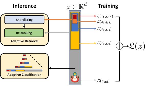
${\rm Matryoshka~Representation~Learning}$ ( ${\rm MRL}$ ) to induce flexibility in the learned representation. ${\rm MRL}$ learns representations of varying capacities within the same high-dimensional vector through explicit optimization of $O(\log(d))$ lower-dimensional vectors in a nested fashion, hence the name ${\rm Matryoshka}$ . ${\rm MRL}$ can be adapted to any existing representation pipeline and is easily extended to many standard tasks in computer vision and natural language processing. Figure 1 illustrates the core idea of ${\rm Matryoshka~Representation~Learning}$ ( ${\rm MRL}$ ) and the adaptive deployment settings of the learned ${\rm Matryoshka~Representations}$ .
<details>
<summary>x3.png Details</summary>
### Visual Description
\n
## Diagram: Adaptive Retrieval and Classification Pipeline
### Overview
This diagram illustrates a pipeline for adaptive retrieval and classification, showing the processes involved in both training and inference stages. The diagram depicts a vertical structure representing a dimensionality reduction or encoding process, with inference and training occurring on either side.
### Components/Axes
The diagram is divided into three main sections:
* **Inference (Left):** Contains two stages: Shortlisting and Re-ranking, leading to Adaptive Retrieval and Adaptive Classification.
* **Central Structure:** A vertical gray rectangle with colored segments representing different levels of dimensionality reduction.
* **Training (Right):** Shows the summation of the encoded representations.
Key labels include:
* `z ∈ ℝᵈ` : Represents the input vector in d-dimensional space.
* `L(z₁:d/16)`, `L(z₁:d/8)`, `L(z₁:d/4)`, `L(z₁:d/2)`, `L(z₁:d)`: Labels indicating different levels of encoded representations.
* `⊕ – Σ(z)`: Represents the summation of encoded representations during training.
* Adaptive Retrieval
* Adaptive Classification
### Detailed Analysis or Content Details
The central structure is a vertical gray rectangle divided into five colored segments from top to bottom: red, blue, yellow, orange, and a red/white patterned base. Each segment is associated with a level of encoded representation `L(z)` with decreasing dimensionality.
* **Red Segment (Top):** Labeled `L(z₁:d/16)`. An orange arrow connects this segment to the "Shortlisting" stage in the Inference section.
* **Blue Segment:** Labeled `L(z₁:d/8)`. An orange arrow connects this segment to the "Re-ranking" stage in the Inference section.
* **Yellow Segment:** Labeled `L(z₁:d/4)`. An orange arrow connects this segment to the "Adaptive Retrieval" stage in the Inference section.
* **Orange Segment:** Labeled `L(z₁:d/2)`. An orange arrow connects this segment to the "Adaptive Classification" stage in the Inference section.
* **Red/White Patterned Segment (Bottom):** Labeled `L(z₁:d)`. An orange arrow connects this segment to the summation symbol `⊕ – Σ(z)` in the Training section.
The Inference section shows a flow from "Shortlisting" to "Re-ranking", then to "Adaptive Retrieval" and "Adaptive Classification". A dashed arrow connects "Adaptive Retrieval" to "Adaptive Classification".
The Training section shows the summation symbol `⊕ – Σ(z)` connected to all the encoded representations via a bracket.
### Key Observations
The diagram highlights a hierarchical encoding process where the input vector `z` is progressively reduced in dimensionality through the layers `L(z)`. The different levels of encoded representations are used for different stages of inference (shortlisting, re-ranking, retrieval, classification). The training process involves summing these encoded representations.
### Interpretation
This diagram represents a machine learning pipeline, likely for information retrieval or classification tasks. The central structure suggests an autoencoder or similar dimensionality reduction technique. The different levels of encoded representations (`L(z)`) likely capture different levels of abstraction or granularity of the input data.
* **Inference:** The inference process uses these encoded representations to first narrow down the search space (shortlisting), then refine the results (re-ranking), and finally retrieve and classify the relevant information.
* **Training:** The training process aims to learn the optimal encoding by minimizing the reconstruction error (summing the encoded representations).
The use of adaptive retrieval and classification suggests that the system can dynamically adjust its retrieval and classification strategies based on the input data. The diagram doesn't provide specific details about the algorithms used, but it provides a high-level overview of the pipeline's architecture. The diagram is conceptual and does not contain numerical data.
</details>
Figure 1:
<details>
<summary>x5.png Details</summary>

### Visual Description
Icon/Small Image (28x28)
</details>
${\rm Matryoshka~Representation~Learning}$ is adaptable to any representation learning setup and begets a ${\rm Matryoshka~Representation}$ $z$ by optimizing the original loss $\mathcal{L}(.)$ at $O(\log(d))$ chosen representation sizes. ${\rm Matryoshka~Representation}$ can be utilized effectively for adaptive deployment across environments and downstream tasks.
The first $m$ -dimensions, $m∈[d]$ , of the ${\rm Matryoshka~Representation}$ is an information-rich low-dimensional vector, at no additional training cost, that is as accurate as an independently trained $m$ -dimensional representation. The information within the ${\rm Matryoshka~Representation}$ increases with the dimensionality creating a coarse-to-fine grained representation, all without significant training or additional deployment overhead. ${\rm MRL}$ equips the representation vector with the desired flexibility and multifidelity that can ensure a near-optimal accuracy-vs-compute trade-off. With these advantages, ${\rm MRL}$ enables adaptive deployment based on accuracy and compute constraints.
The ${\rm Matryoshka~Representations}$ improve efficiency for large-scale classification and retrieval without any significant loss of accuracy. While there are potentially several applications of coarse-to-fine ${\rm Matryoshka~Representations}$ , in this work we focus on two key building blocks of real-world ML systems: large-scale classification and retrieval. For classification, we use adaptive cascades with the variable-size representations from a model trained with ${\rm MRL}$ , significantly reducing the average dimension of embeddings needed to achieve a particular accuracy. For example, on ImageNet-1K, ${\rm MRL}$ + adaptive classification results in up to a $14×$ smaller representation size at the same accuracy as baselines (Section 4.2.1). Similarly, we use ${\rm MRL}$ in an adaptive retrieval system. Given a query, we shortlist retrieval candidates using the first few dimensions of the query embedding, and then successively use more dimensions to re-rank the retrieved set. A simple implementation of this approach leads to $128×$ theoretical (in terms of FLOPS) and $14×$ wall-clock time speedups compared to a single-shot retrieval system that uses a standard embedding vector; note that ${\rm MRL}$ ’s retrieval accuracy is comparable to that of single-shot retrieval (Section 4.3.1). Finally, as ${\rm MRL}$ explicitly learns coarse-to-fine representation vectors, intuitively it should share more semantic information among its various dimensions (Figure 5). This is reflected in up to $2\%$ accuracy gains in long-tail continual learning settings while being as robust as the original embeddings. Furthermore, due to its coarse-to-fine grained nature, ${\rm MRL}$ can also be used as method to analyze hardness of classification among instances and information bottlenecks.
We make the following key contributions:
1. We introduce
<details>
<summary>x6.png Details</summary>

### Visual Description
Icon/Small Image (28x28)
</details>
${\rm Matryoshka~Representation~Learning}$ ( ${\rm MRL}$ ) to obtain flexible representations ( ${\rm Matryoshka~Representations}$ ) for adaptive deployment (Section 3).
1. Up to $14×$ faster yet accurate large-scale classification and retrieval using ${\rm MRL}$ (Section 4).
1. Seamless adaptation of ${\rm MRL}$ across modalities (vision - ResNet & ViT, vision + language - ALIGN, language - BERT) and to web-scale data (ImageNet-1K/4K, JFT-300M and ALIGN data).
1. Further analysis of ${\rm MRL}$ ’s representations in the context of other downstream tasks (Section 5).
2 Related Work
Representation Learning.
Large-scale datasets like ImageNet [16, 76] and JFT [85] enabled the learning of general purpose representations for computer vision [4, 98]. These representations are typically learned through supervised and un/self-supervised learning paradigms. Supervised pretraining [29, 51, 82] casts representation learning as a multi-class/label classification problem, while un/self-supervised learning learns representation via proxy tasks like instance classification [97] and reconstruction [31, 63]. Recent advances [12, 30] in contrastive learning [27] enabled learning from web-scale data [21] that powers large-capacity cross-modal models [18, 46, 71, 101]. Similarly, natural language applications are built [40] on large language models [8] that are pretrained [68, 75] in a un/self-supervised fashion with masked language modelling [19] or autoregressive training [70].
<details>
<summary>x7.png Details</summary>

### Visual Description
Icon/Small Image (28x28)
</details>
${\rm Matryoshka~Representation~Learning}$ ( ${\rm MRL}$ ) is complementary to all these setups and can be adapted with minimal overhead (Section 3). ${\rm MRL}$ equips representations with multifidelity at no additional cost which enables adaptive deployment based on the data and task (Section 4).
Efficient Classification and Retrieval.
Efficiency in classification and retrieval during inference can be studied with respect to the high yet constant deep featurization costs or the search cost which scales with the size of the label space and data. Efficient neural networks address the first issue through a variety of algorithms [25, 54] and design choices [39, 53, 87]. However, with a strong featurizer, most of the issues with scale are due to the linear dependence on number of labels ( $L$ ), size of the data ( $N$ ) and representation size ( $d$ ), stressing RAM, disk and processor all at the same time.
The sub-linear complexity dependence on number of labels has been well studied in context of compute [3, 43, 69] and memory [20] using Approximate Nearest Neighbor Search (ANNS) [62] or leveraging the underlying hierarchy [17, 55]. In case of the representation size, often dimensionality reduction [77, 88], hashing techniques [14, 52, 78] and feature selection [64] help in alleviating selective aspects of the $O(d)$ scaling at a cost of significant drops in accuracy. Lastly, most real-world search systems [11, 15] are often powered by large-scale embedding based retrieval [10, 66] that scales in cost with the ever increasing web-data. While categorization [89, 99] clusters similar things together, it is imperative to be equipped with retrieval capabilities that can bring forward every instance [7]. Approximate Nearest Neighbor Search (ANNS) [42] makes it feasible with efficient indexing [14] and traversal [5, 6] to present the users with the most similar documents/images from the database for a requested query. Widely adopted HNSW [62] ( $O(d\log(N))$ ) is as accurate as exact retrieval ( $O(dN)$ ) at the cost of a graph-based index overhead for RAM and disk [44].
${\rm MRL}$ tackles the linear dependence on embedding size, $d$ , by learning multifidelity ${\rm Matryoshka~Representations}$ . Lower-dimensional ${\rm Matryoshka~Representations}$ are as accurate as independently trained counterparts without the multiple expensive forward passes. ${\rm Matryoshka~Representations}$ provide an intermediate abstraction between high-dimensional vectors and their efficient ANNS indices through the adaptive embeddings nested within the original representation vector (Section 4). All other aforementioned efficiency techniques are complementary and can be readily applied to the learned ${\rm Matryoshka~Representations}$ obtained from ${\rm MRL}$ .
Several works in efficient neural network literature [9, 93, 100] aim at packing neural networks of varying capacity within the same larger network. However, the weights for each progressively smaller network can be different and often require distinct forward passes to isolate the final representations. This is detrimental for adaptive inference due to the need for re-encoding the entire retrieval database with expensive sub-net forward passes of varying capacities. Several works [23, 26, 65, 59] investigate the notions of intrinsic dimensionality and redundancy of representations and objective spaces pointing to minimum description length [74]. Finally, ordered representations proposed by Rippel et al. [73] use nested dropout in the context of autoencoders to learn nested representations. ${\rm MRL}$ differentiates itself in formulation by optimizing only for $O(\log(d))$ nesting dimensions instead of $O(d)$ . Despite this, ${\rm MRL}$ diffuses information to intermediate dimensions interpolating between the optimized ${\rm Matryoshka~Representation}$ sizes accurately (Figure 5); making web-scale feasible.
3
<details>
<summary>x8.png Details</summary>

### Visual Description
Icon/Small Image (28x28)
</details>
${\rm Matryoshka~Representation~Learning}$
For $d∈\mathbb{N}$ , consider a set $\mathcal{M}⊂[d]$ of representation sizes. For a datapoint $x$ in the input domain $\mathcal{X}$ , our goal is to learn a $d$ -dimensional representation vector $z∈\mathbb{R}^{d}$ . For every $m∈\mathcal{M}$ , ${\rm Matryoshka~Representation~Learning}$ ( ${\rm MRL}$ ) enables each of the first $m$ dimensions of the embedding vector, $z_{1:m}∈\mathbb{R}^{m}$ to be independently capable of being a transferable and general purpose representation of the datapoint $x$ . We obtain $z$ using a deep neural network $F(\,·\,;\theta_{F})\colon\mathcal{X}→\mathbb{R}^{d}$ parameterized by learnable weights $\theta_{F}$ , i.e., $z\coloneqq F(x;\theta_{F})$ . The multi-granularity is captured through the set of the chosen dimensions $\mathcal{M}$ , that contains less than $\log(d)$ elements, i.e., $\lvert\mathcal{M}\rvert≤\left\lfloor\log(d)\right\rfloor$ . The usual set $\mathcal{M}$ consists of consistent halving until the representation size hits a low information bottleneck. We discuss the design choices in Section 4 for each of the representation learning settings.
For the ease of exposition, we present the formulation for fully supervised representation learning via multi-class classification. ${\rm Matryoshka~Representation~Learning}$ modifies the typical setting to become a multi-scale representation learning problem on the same task. For example, we train ResNet50 [29] on ImageNet-1K [76] which embeds a $224× 224$ pixel image into a $d=2048$ representation vector and then passed through a linear classifier to make a prediction, $\hat{y}$ among the $L=1000$ labels. For ${\rm MRL}$ , we choose $\mathcal{M}=\{8,16,...,1024,2048\}$ as the nesting dimensions.
Suppose we are given a labelled dataset $\mathcal{D}=\{(x_{1},y_{1}),...,(x_{N},y_{N})\}$ where $x_{i}∈\mathcal{X}$ is an input point and $y_{i}∈[L]$ is the label of $x_{i}$ for all $i∈[N]$ . ${\rm MRL}$ optimizes the multi-class classification loss for each of the nested dimension $m∈\mathcal{M}$ using standard empirical risk minimization using a separate linear classifier, parameterized by $\mathbf{W}^{(m)}∈\mathbb{R}^{L× m}$ . All the losses are aggregated after scaling with their relative importance $\left(c_{m}≥ 0\right)_{m∈\mathcal{M}}$ respectively. That is, we solve
$$
\min_{\left\{\mathbf{W}^{(m)}\right\}_{m\in\mathcal{M}},\ \theta_{F}}\frac{1}{N}\sum_{i\in[N]}\sum_{m\in\mathcal{M}}c_{m}\cdot{\cal L}\left(\mathbf{W}^{(m)}\cdot F(x_{i};\theta_{F})_{1:m}\ ;\ y_{i}\right)\ , \tag{1}
$$
where ${\cal L}\colon\mathbb{R}^{L}×[L]→\mathbb{R}_{+}$ is the multi-class softmax cross-entropy loss function. This is a standard optimization problem that can be solved using sub-gradient descent methods. We set all the importance scales, $c_{m}=1$ for all $m∈\mathcal{M}$ ; see Section 5 for ablations. Lastly, despite only optimizing for $O(\log(d))$ nested dimensions, ${\rm MRL}$ results in accurate representations, that interpolate, for dimensions that fall between the chosen granularity of the representations (Section 4.2).
We call this formulation as ${\rm Matryoshka~Representation~Learning}$ ( ${\rm MRL}$ ). A natural way to make this efficient is through weight-tying across all the linear classifiers, i.e., by defining $\mathbf{W}^{(m)}=\mathbf{W}_{1:m}$ for a set of common weights $\mathbf{W}∈\mathbb{R}^{L× d}$ . This would reduce the memory cost due to the linear classifiers by almost half, which would be crucial in cases of extremely large output spaces [89, 99]. This variant is called Efficient ${\rm Matryoshka~Representation~Learning}$ ( ${\rm MRL\text{--}E}$ ). Refer to Alg 1 and Alg 2 in Appendix A for the building blocks of ${\rm Matryoshka~Representation~Learning}$ ( ${\rm MRL}$ ).
Adaptation to Learning Frameworks.
${\rm MRL}$ can be adapted seamlessly to most representation learning frameworks at web-scale with minimal modifications (Section 4.1). For example, ${\rm MRL}$ ’s adaptation to masked language modelling reduces to ${\rm MRL\text{--}E}$ due to the weight-tying between the input embedding matrix and the linear classifier. For contrastive learning, both in context of vision & vision + language, ${\rm MRL}$ is applied to both the embeddings that are being contrasted with each other. The presence of normalization on the representation needs to be handled independently for each of the nesting dimension for best results (see Appendix C for more details).
4 Applications
In this section, we discuss ${\rm Matryoshka~Representation~Learning}$ ( ${\rm MRL}$ ) for a diverse set of applications along with an extensive evaluation of the learned multifidelity representations. Further, we showcase the downstream applications of the learned ${\rm Matryoshka~Representations}$ for flexible large-scale deployment through (a) Adaptive Classification (AC) and (b) Adaptive Retrieval (AR).
<details>
<summary>x9.png Details</summary>
### Visual Description
## Line Chart: Top-1 Accuracy vs. Representation Size
### Overview
This line chart depicts the relationship between "Representation Size" and "Top-1 Accuracy" for six different models: MRL, MRL-E, FF, SVD, Slim. Net, and Rand. LP. The chart illustrates how the accuracy of each model changes as the size of the representation increases.
### Components/Axes
* **X-axis:** "Representation Size" - Scale ranges from 8 to 2048, with markers at 8, 16, 32, 64, 128, 256, 512, 1024, and 2048.
* **Y-axis:** "Top-1 Accuracy (%)" - Scale ranges from 40% to 80%, with markers at 40, 50, 60, 70, and 80.
* **Legend:** Located in the top-right corner, identifying each line with a color and label:
* MRL (Blue)
* MRL-E (Orange)
* FF (Green)
* SVD (Red)
* Slim. Net (Purple)
* Rand. LP (Brown)
### Detailed Analysis
Here's a breakdown of each line's trend and approximate data points, verifying color consistency with the legend:
* **MRL (Blue):** The line starts at approximately 68% accuracy at a representation size of 8, rises quickly to around 74% at size 16, plateaus around 76-77% between sizes 32 and 512, and remains relatively stable at approximately 77-78% for sizes 1024 and 2048.
* **MRL-E (Orange):** Starts at approximately 57% accuracy at size 8, increases rapidly to around 71% at size 16, reaches a peak of approximately 74% at size 64, and then plateaus around 74-75% for larger representation sizes.
* **FF (Green):** Begins at approximately 62% accuracy at size 8, increases steadily to around 72% at size 64, and then plateaus around 73-74% for larger representation sizes.
* **SVD (Red):** Starts at approximately 42% accuracy at size 8, exhibits a steep increase to around 68% at size 64, continues to rise to approximately 76% at size 256, and then plateaus around 77-78% for larger representation sizes.
* **Slim. Net (Purple):** Starts at approximately 65% accuracy at size 8, increases to around 73% at size 32, and then rises more gradually to approximately 76% at size 512, remaining relatively stable at around 76-77% for larger sizes.
* **Rand. LP (Brown):** Starts at approximately 42% accuracy at size 8, increases steadily to around 65% at size 128, and then rises more rapidly to approximately 74% at size 512, and plateaus around 75-76% for larger sizes.
### Key Observations
* The "MRL" model consistently achieves the highest accuracy across all representation sizes, particularly at larger sizes.
* "SVD" shows the most significant improvement in accuracy as representation size increases, starting from the lowest accuracy and eventually reaching a similar level to "MRL".
* "MRL-E", "FF", and "Slim. Net" exhibit similar accuracy trends, plateauing at around 73-76% for larger representation sizes.
* "Rand. LP" starts with the lowest accuracy but shows a substantial increase with larger representation sizes, though it remains slightly below the other models.
### Interpretation
The data suggests that increasing the representation size generally improves the Top-1 accuracy of these models. However, the rate of improvement diminishes as the representation size grows larger, indicating a point of diminishing returns. The "MRL" model appears to be the most effective in leveraging larger representation sizes, while "SVD" benefits the most from increasing representation size, starting from a lower baseline. The plateauing of accuracy for most models suggests that other factors, such as model architecture or training data, may become more limiting as representation size increases. The differences in accuracy between the models highlight the importance of model design and optimization for achieving high performance. The "Rand. LP" model's initial low accuracy and subsequent improvement suggest that it may require larger representations to effectively capture the underlying patterns in the data.
</details>
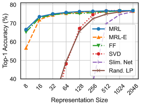
Figure 2: ImageNet-1K linear classification accuracy of ResNet50 models. ${\rm MRL}$ is as accurate as the independently trained FF models for every representation size.
<details>
<summary>x10.png Details</summary>
### Visual Description
## Line Chart: 1-NN Accuracy vs. Representation Size
### Overview
This image presents a line chart illustrating the relationship between representation size and 1-Nearest Neighbor (1-NN) accuracy for six different methods. The chart displays how accuracy changes as the representation size increases, ranging from 8 to 2048.
### Components/Axes
* **X-axis:** Representation Size (scaled logarithmically). Markers are present at 8, 16, 32, 64, 128, 256, 512, 1024, and 2048.
* **Y-axis:** 1-NN Accuracy (%). The scale ranges from 40% to 70%.
* **Legend:** Located in the top-right corner, identifying six data series:
* MRL (Blue, solid line with circle markers)
* MRL-E (Orange, dashed line with square markers)
* FF (Green, dotted line with triangle markers)
* SVD (Red, dotted line with diamond markers)
* Slim. Net (Purple, dashed line with plus markers)
* Rand. FS (Brown, solid line with cross markers)
* **Gridlines:** Present to aid in reading values.
### Detailed Analysis
Here's a breakdown of each data series, noting trends and approximate values:
* **MRL (Blue):** The line starts at approximately 68% accuracy at a representation size of 8, increases slightly to around 71% at 16, plateaus around 72% from 32 to 2048.
* **MRL-E (Orange):** Starts at approximately 58% at 8, rises to around 68% at 16, then plateaus around 70% from 32 to 2048.
* **FF (Green):** Begins at approximately 64% at 8, increases to around 69% at 16, and then plateaus around 71% from 32 to 2048.
* **SVD (Red):** Shows a significant increase in accuracy with increasing representation size. Starts at approximately 43% at 8, rises to around 59% at 16, 68% at 64, 71% at 128, and plateaus around 72% from 256 to 2048.
* **Slim. Net (Purple):** Starts at approximately 60% at 8, increases to around 65% at 16, and then rises more steeply to around 68% at 128, and plateaus around 70% from 256 to 2048.
* **Rand. FS (Brown):** Starts at approximately 40% at 8, increases rapidly to around 60% at 64, 68% at 128, and plateaus around 71% from 256 to 2048.
### Key Observations
* All methods achieve relatively high accuracy (above 70%) at larger representation sizes (256 and above).
* SVD and Rand. FS show the most significant improvement in accuracy as representation size increases, particularly in the lower range (8-128).
* MRL, MRL-E, and FF exhibit relatively stable accuracy across all representation sizes, with minimal improvement beyond a size of 32.
* The performance gap between the methods narrows as representation size increases.
### Interpretation
The data suggests that increasing the representation size generally improves 1-NN accuracy, but the rate of improvement varies significantly depending on the method used. Methods like SVD and Rand. FS, which initially have lower accuracy, benefit the most from larger representation sizes. This indicates that these methods require more data to effectively capture the underlying patterns in the data. Conversely, MRL, MRL-E, and FF achieve high accuracy even with small representation sizes, suggesting they are more efficient at extracting relevant features. The plateauing of accuracy at larger representation sizes for all methods suggests a point of diminishing returns, where further increasing the representation size does not lead to substantial gains in performance. This could be due to overfitting or the inherent limitations of the 1-NN algorithm. The logarithmic scale on the x-axis emphasizes the importance of the initial increase in representation size for methods like SVD and Rand. FS, where the largest gains are observed in the lower range.
</details>
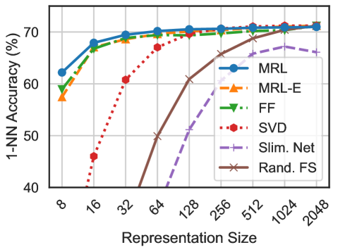
Figure 3: ImageNet-1K 1-NN accuracy of ResNet50 models measuring the representation quality for downstream task. ${\rm MRL}$ outperforms all the baselines across all representation sizes.
4.1 Representation Learning
We adapt ${\rm Matryoshka~Representation~Learning}$ ( ${\rm MRL}$ ) to various representation learning setups (a) Supervised learning for vision: ResNet50 [29] on ImageNet-1K [76] and ViT-B/16 [22] on JFT-300M [85], (b) Contrastive learning for vision + language: ALIGN model with ViT-B/16 vision encoder and BERT language encoder on ALIGN data [46] and (c) Masked language modelling: BERT [19] on English Wikipedia and BooksCorpus [102]. Please refer to Appendices B and C for details regarding the model architectures, datasets and training specifics.
We do not search for best hyper-parameters for all ${\rm MRL}$ experiments but use the same hyper-parameters as the independently trained baselines. ResNet50 outputs a $2048$ -dimensional representation while ViT-B/16 and BERT-Base output $768$ -dimensional embeddings for each data point. We use $\mathcal{M}=\{8,16,32,64,128,256,512,1024,2048\}$ and $\mathcal{M}=\{12,24,48,96,192,384,768\}$ as the explicitly optimized nested dimensions respectively. Lastly, we extensively compare the ${\rm MRL}$ and ${\rm MRL\text{--}E}$ models to independently trained low-dimensional (fixed feature) representations (FF), dimensionality reduction (SVD), sub-net method (slimmable networks [100]) and randomly selected features of the highest capacity FF model.
In section 4.2, we evaluate the quality and capacity of the learned representations through linear classification/probe (LP) and 1-nearest neighbour (1-NN) accuracy. Experiments show that ${\rm MRL}$ models remove the dependence on $|\mathcal{M}|$ resource-intensive independently trained models for the coarse-to-fine representations while being as accurate. Lastly, we show that despite optimizing only for $|\mathcal{M}|$ dimensions, ${\rm MRL}$ models diffuse the information, in an interpolative fashion, across all the $d$ dimensions providing the finest granularity required for adaptive deployment.
4.2 Classification
Figure 3 compares the linear classification accuracy of ResNet50 models trained and evaluated on ImageNet-1K. ResNet50– ${\rm MRL}$ model is at least as accurate as each FF model at every representation size in $\mathcal{M}$ while ${\rm MRL\text{--}E}$ is within $1\%$ starting from $16$ -dim. Similarly, Figure 3 showcases the comparison of learned representation quality through 1-NN accuracy on ImageNet-1K (trainset with 1.3M samples as the database and validation set with 50K samples as the queries). ${\rm Matryoshka~Representations}$ are up to $2\%$ more accurate than their fixed-feature counterparts for the lower-dimensions while being as accurate elsewhere. 1-NN accuracy is an excellent proxy, at no additional training cost, to gauge the utility of learned representations in the downstream tasks.
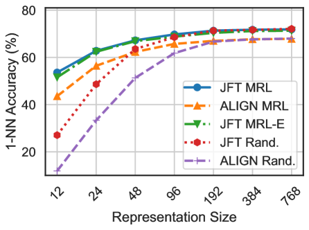
We also evaluate the quality of the representations from training ViT-B/16 on JFT-300M alongside the ViT-B/16 vision encoder of the ALIGN model – two web-scale setups. Due to the expensive nature of these experiments, we only train the highest capacity fixed feature model and choose random features for evaluation in lower-dimensions. Web-scale is a compelling setting for ${\rm MRL}$ due to its relatively inexpensive training overhead while providing multifidelity representations for downstream tasks. Figure 5, evaluated with 1-NN on ImageNet-1K, shows that all the ${\rm MRL}$ models for JFT and ALIGN are highly accurate while providing an excellent cost-vs-accuracy trade-off at lower-dimensions. These experiments show that ${\rm MRL}$ seamlessly scales to large-scale models and web-scale datasets while providing the otherwise prohibitively expensive multi-granularity in the process. We also have similar observations when pretraining BERT; please see Appendix D.2 for more details.
<details>
<summary>x11.png Details</summary>
### Visual Description
## Line Chart: 1-NN Accuracy vs. Representation Size
### Overview
This line chart displays the 1-Nearest Neighbor (1-NN) accuracy for different representation sizes, comparing several models: JFT MRL, ALIGN MRL, JFT MRL-E, JFT Rand., and ALIGN Rand. The x-axis represents the representation size, and the y-axis represents the 1-NN accuracy in percentage.
### Components/Axes
* **X-axis:** Representation Size (with markers at 12, 24, 48, 96, 192, 384, 768)
* **Y-axis:** 1-NN Accuracy (%) (scale from 0 to 80, increments of 10)
* **Legend:** Located in the top-right corner, containing the following labels and corresponding colors:
* JFT MRL (Blue)
* ALIGN MRL (Orange)
* JFT MRL-E (Green)
* JFT Rand. (Red)
* ALIGN Rand. (Purple)
### Detailed Analysis
* **JFT MRL (Blue Line):** The line slopes upward sharply from 12 to 48, then plateaus, reaching approximately 72% accuracy at a representation size of 48, and remaining relatively stable around 72-74% for larger representation sizes.
* At Representation Size 12: ~54%
* At Representation Size 24: ~64%
* At Representation Size 48: ~72%
* At Representation Size 96: ~73%
* At Representation Size 192: ~73%
* At Representation Size 384: ~73%
* At Representation Size 768: ~73%
* **ALIGN MRL (Orange Line):** The line shows a similar upward trend to JFT MRL, but starts at a lower accuracy. It reaches approximately 68% accuracy at a representation size of 48 and plateaus around 70-72% for larger sizes.
* At Representation Size 12: ~42%
* At Representation Size 24: ~55%
* At Representation Size 48: ~68%
* At Representation Size 96: ~70%
* At Representation Size 192: ~71%
* At Representation Size 384: ~71%
* At Representation Size 768: ~71%
* **JFT MRL-E (Green Line):** This line starts with a similar accuracy to ALIGN MRL at a representation size of 12, and increases steadily, reaching approximately 70% accuracy at a representation size of 48. It plateaus around 71-72% for larger sizes.
* At Representation Size 12: ~50%
* At Representation Size 24: ~60%
* At Representation Size 48: ~70%
* At Representation Size 96: ~71%
* At Representation Size 192: ~71%
* At Representation Size 384: ~71%
* At Representation Size 768: ~71%
* **JFT Rand. (Red Line):** This line exhibits a steep upward trend, starting from approximately 24% at a representation size of 12 and reaching approximately 70% accuracy at a representation size of 384. It plateaus around 71-72% for larger sizes.
* At Representation Size 12: ~24%
* At Representation Size 24: ~34%
* At Representation Size 48: ~48%
* At Representation Size 96: ~60%
* At Representation Size 192: ~67%
* At Representation Size 384: ~71%
* At Representation Size 768: ~71%
* **ALIGN Rand. (Purple Line):** This line shows the most significant upward trend, starting from a very low accuracy at a representation size of 12 and increasing rapidly to approximately 65% at a representation size of 192. It plateaus around 70-72% for larger sizes.
* At Representation Size 12: ~10%
* At Representation Size 24: ~20%
* At Representation Size 48: ~32%
* At Representation Size 96: ~46%
* At Representation Size 192: ~65%
* At Representation Size 384: ~71%
* At Representation Size 768: ~71%
### Key Observations
* All models exhibit diminishing returns in accuracy as the representation size increases beyond 48.
* JFT MRL consistently achieves the highest accuracy across all representation sizes.
* ALIGN Rand. shows the most significant improvement in accuracy with increasing representation size, starting from the lowest accuracy.
* The "Rand." models (JFT Rand. and ALIGN Rand.) initially perform worse than their corresponding "MRL" counterparts but converge towards similar accuracy levels at larger representation sizes.
### Interpretation
The chart demonstrates the relationship between representation size and 1-NN accuracy for different models. The plateauing of accuracy at larger representation sizes suggests that the models have reached a point of diminishing returns, where increasing the representation size does not significantly improve performance. The differences in accuracy between the models indicate varying levels of effectiveness in capturing relevant information from the data. The convergence of the "Rand." models towards the "MRL" models at larger representation sizes suggests that random representations can become effective with sufficient dimensionality. This data could be used to optimize model selection and representation size for a given task, balancing accuracy with computational cost. The fact that all lines converge suggests that the underlying data has a limited amount of information that can be extracted, and beyond a certain point, increasing the representation size does not reveal new patterns.
</details>
Figure 4: ImageNet-1K 1-NN accuracy for ViT-B/16 models trained on JFT-300M & as part of ALIGN. ${\rm MRL}$ scales seamlessly to web-scale with minimal training overhead.
<details>
<summary>x12.png Details</summary>
### Visual Description
## Line Chart: 1-NN Accuracy vs. Representation Size
### Overview
This image presents a line chart comparing the 1-Nearest Neighbor (1-NN) accuracy of several models as a function of representation size. The chart displays performance for both standard models and their "Int" (likely integer quantized) versions.
### Components/Axes
* **X-axis:** Representation Size (logarithmic scale). Markers are present at 8, 16, 32, 64, 128, 256, 512, 1024, and 2048.
* **Y-axis:** 1-NN Accuracy (%). The scale ranges from approximately 45% to 75%.
* **Legend:** Located in the top-right corner. Contains the following entries:
* VIT-ALIGN (green dashed line)
* ViT-JFT (blue solid line)
* RN50-1N1K (purple dashed-dotted line)
* VIT-ALIGN-Int (red downward-pointing triangle)
* ViT-JFT-Int (pink circle)
* RN50-1N1K-Int (red square)
### Detailed Analysis
The chart shows the 1-NN accuracy for each model as the representation size increases.
* **VIT-ALIGN (green dashed line):** Starts at approximately 45% accuracy at a representation size of 8, increases rapidly to around 68% at a size of 64, and then plateaus around 68-70% for larger representation sizes.
* **ViT-JFT (blue solid line):** Begins at approximately 65% accuracy at a representation size of 8, increases steadily to around 72% at a size of 64, and then plateaus around 72-73% for larger representation sizes.
* **RN50-1N1K (purple dashed-dotted line):** Starts at approximately 67% accuracy at a representation size of 8, increases to around 71% at a size of 64, and then plateaus around 72-73% for larger representation sizes.
* **VIT-ALIGN-Int (red downward-pointing triangle):** Starts at approximately 52% accuracy at a representation size of 8, increases rapidly to around 70% at a size of 64, and then plateaus around 70-72% for larger representation sizes.
* **ViT-JFT-Int (pink circle):** Begins at approximately 68% accuracy at a representation size of 8, increases steadily to around 73% at a size of 64, and then plateaus around 73-74% for larger representation sizes.
* **RN50-1N1K-Int (red square):** Starts at approximately 70% accuracy at a representation size of 8, increases to around 73% at a size of 64, and then plateaus around 73-74% for larger representation sizes.
### Key Observations
* The "Int" versions of the models generally have lower accuracy than their standard counterparts at smaller representation sizes (8-32).
* As representation size increases, the accuracy of the "Int" models converges towards the accuracy of the standard models.
* All models exhibit diminishing returns in accuracy beyond a representation size of 64.
* ViT-JFT and RN50-1N1K consistently achieve higher accuracy than VIT-ALIGN across all representation sizes.
* RN50-1N1K-Int consistently achieves the highest accuracy.
### Interpretation
The data suggests that increasing the representation size improves the 1-NN accuracy of these models, but there is a point of diminishing returns. The "Int" versions of the models, which likely use integer quantization to reduce memory footprint and computational cost, initially suffer a performance penalty compared to the standard models. However, this penalty is mitigated as the representation size increases, indicating that the larger representation provides sufficient information to overcome the quantization effects. The convergence of the "Int" models towards the standard models suggests that integer quantization is a viable strategy for model compression, especially when combined with larger representation sizes. The consistently higher performance of ViT-JFT and RN50-1N1K suggests that these architectures are more effective for this particular task or dataset. The fact that RN50-1N1K-Int achieves the highest accuracy overall indicates that it is the most efficient and accurate model in this comparison.
</details>
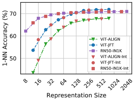
Figure 5: Despite optimizing ${\rm MRL}$ only for $O(\log(d))$ dimensions for ResNet50 and ViT-B/16 models; the accuracy in the intermediate dimensions shows interpolating behaviour.
Our experiments also show that post-hoc compression (SVD), linear probe on random features, and sub-net style slimmable networks drastically lose accuracy compared to ${\rm MRL}$ as the representation size decreases. Finally, Figure 5 shows that, while ${\rm MRL}$ explicitly optimizes $O(\log(d))$ nested representations – removing the $O(d)$ dependence [73] –, the coarse-to-fine grained information is interpolated across all $d$ dimensions providing highest flexibility for adaptive deployment.
4.2.1 Adaptive Classification
The flexibility and coarse-to-fine granularity within ${\rm Matryoshka~Representations}$ allows model cascades [90] for Adaptive Classification (AC) [28]. Unlike standard model cascades [95], ${\rm MRL}$ does not require multiple expensive neural network forward passes. To perform AC with an ${\rm MRL}$ trained model, we learn thresholds on the maximum softmax probability [33] for each nested classifier on a holdout validation set. We then use these thresholds to decide when to transition to the higher dimensional representation (e.g $8→ 16→ 32$ ) of the ${\rm MRL}$ model. Appendix D.1 discusses the implementation and learning of thresholds for cascades used for adaptive classification in detail.
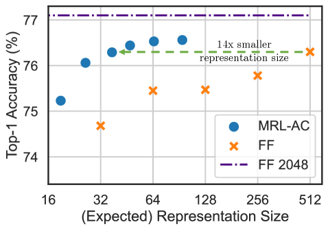
Figure 7 shows the comparison between cascaded ${\rm MRL}$ representations ( ${\rm MRL}$ –AC) and independently trained fixed feature (FF) models on ImageNet-1K with ResNet50. We computed the expected representation size for ${\rm MRL}$ –AC based on the final dimensionality used in the cascade. We observed that ${\rm MRL}$ –AC was as accurate, $76.30\%$ , as a 512-dimensional FF model but required an expected dimensionality of $\sim 37$ while being only $0.8\%$ lower than the 2048-dimensional FF baseline. Note that all ${\rm MRL}$ –AC models are significantly more accurate than the FF baselines at comparable representation sizes. ${\rm MRL}$ –AC uses up to $\sim 14×$ smaller representation size for the same accuracy which affords computational efficiency as the label space grows [89]. Lastly, our results with ${\rm MRL}$ –AC indicate that instances and classes vary in difficulty which we analyze in Section 5 and Appendix J.
4.3 Retrieval
Nearest neighbour search with learned representations powers a plethora of retrieval and search applications [15, 91, 11, 66]. In this section, we discuss the image retrieval performance of the pretrained ResNet50 models (Section 4.1) on two large-scale datasets ImageNet-1K [76] and ImageNet-4K. ImageNet-1K has a database size of $\sim$ 1.3M and a query set of 50K samples uniformly spanning 1000 classes. We also introduce ImageNet-4K which has a database size of $\sim$ 4.2M and query set of $\sim$ 200K samples uniformly spanning 4202 classes (see Appendix B for details). A single forward pass on ResNet50 costs 4 GFLOPs while exact retrieval costs 2.6 GFLOPs per query for ImageNet-1K. Although retrieval overhead is $40\%$ of the total cost, retrieval cost grows linearly with the size of the database. ImageNet-4K presents a retrieval benchmark where the exact search cost becomes the computational bottleneck ( $8.6$ GFLOPs per query). In both these settings, the memory and disk usage are also often bottlenecked by the large databases. However, in most real-world applications exact search, $O(dN)$ , is replaced with an approximate nearest neighbor search (ANNS) method like HNSW [62], $O(d\log(N))$ , with minimal accuracy drop at the cost of additional memory overhead.
The goal of image retrieval is to find images that belong to the same class as the query using representations obtained from a pretrained model. In this section, we compare retrieval performance using mean Average Precision @ 10 (mAP@ $10$ ) which comprehensively captures the setup of relevant image retrieval at scale. We measure the cost per query using exact search in MFLOPs. All embeddings are unit normalized and retrieved using the L2 distance metric. Lastly, we report an extensive set of metrics spanning mAP@ $k$ and P@ $k$ for $k=\{10,25,50,100\}$ and real-world wall-clock times for exact search and HNSW. See Appendices E and F for more details.
<details>
<summary>x13.png Details</summary>
### Visual Description
\n
## Chart: Top-1 Accuracy vs. Representation Size
### Overview
This chart compares the Top-1 Accuracy of two models, MRL-AC and FF, across varying representation sizes. It also shows the performance of a FF 2048 model as a horizontal reference line. The chart demonstrates how accuracy changes with representation size for each model.
### Components/Axes
* **X-axis:** "(Expected) Representation Size" - Scale ranges from 16 to 512, with markers at 16, 32, 64, 128, 256, and 512.
* **Y-axis:** "Top-1 Accuracy (%)" - Scale ranges from 74% to 77%, with gridlines at 0.5% intervals.
* **Data Series:**
* MRL-AC (Blue circles)
* FF (Orange crosses)
* FF 2048 (Purple dashed line)
* **Legend:** Located in the bottom-right corner.
* Blue circle: MRL-AC
* Orange cross: FF
* Purple dashed line: FF 2048
* **Annotation:** "14x smaller representation size" with a green arrow pointing from the FF line to the MRL-AC line.
### Detailed Analysis
**MRL-AC (Blue Circles):**
The MRL-AC line shows an upward trend, indicating increasing accuracy with increasing representation size.
* At Representation Size 16: Approximately 75.2% accuracy.
* At Representation Size 32: Approximately 76.2% accuracy.
* At Representation Size 64: Approximately 76.8% accuracy.
* At Representation Size 128: Approximately 77.0% accuracy.
* At Representation Size 256: Approximately 77.0% accuracy.
* At Representation Size 512: Approximately 76.8% accuracy.
**FF (Orange Crosses):**
The FF line shows a more erratic pattern.
* At Representation Size 16: Approximately 74.8% accuracy.
* At Representation Size 32: Approximately 75.2% accuracy.
* At Representation Size 64: Approximately 75.6% accuracy.
* At Representation Size 128: Approximately 76.0% accuracy.
* At Representation Size 256: Approximately 76.4% accuracy.
* At Representation Size 512: Approximately 76.2% accuracy.
**FF 2048 (Purple Dashed Line):**
This line is horizontal at approximately 77.2% accuracy across all representation sizes.
### Key Observations
* MRL-AC consistently outperforms FF across all representation sizes.
* MRL-AC reaches a plateau in accuracy around a representation size of 128, with minimal improvement at larger sizes.
* FF shows a gradual increase in accuracy with increasing representation size, but remains below MRL-AC.
* The annotation highlights that MRL-AC achieves comparable accuracy to FF 2048 with a representation size that is 14 times smaller.
* The FF line appears to slightly decrease in accuracy at the largest representation size (512).
### Interpretation
The data suggests that MRL-AC is a more efficient model than FF, achieving similar or better accuracy with significantly smaller representation sizes. This is highlighted by the "14x smaller representation size" annotation, indicating a substantial reduction in computational cost or memory usage. The plateau in MRL-AC's accuracy suggests that increasing the representation size beyond a certain point (around 128) does not yield significant performance gains. The FF model, while improving with larger representation sizes, does not reach the same level of accuracy as MRL-AC. The slight dip in FF accuracy at 512 could indicate overfitting or diminishing returns. Overall, the chart demonstrates the effectiveness of MRL-AC in achieving high accuracy with a compact representation, making it a potentially advantageous choice for resource-constrained environments.
</details>
Figure 6: Adaptive classification on ${\rm MRL}$ ResNet50 using cascades results in $14×$ smaller representation size for the same level of accuracy on ImageNet-1K ( $\sim 37$ vs $512$ dims for $76.3\%$ ).
<details>
<summary>x14.png Details</summary>
### Visual Description
## Line Chart: mAP@10 vs. Representation Size
### Overview
This image presents a line chart illustrating the relationship between "Representation Size" and "mAP@10" (mean Average Precision at 10) for six different methods: MRL, MRL-E, FF, SVD, Slim. Net, and Rand. FS. The chart displays how the performance metric (mAP@10) changes as the representation size increases.
### Components/Axes
* **X-axis:** "Representation Size" with values ranging from 8 to 2048. The scale is logarithmic, with markers at 8, 16, 32, 64, 128, 256, 512, 1024, and 2048.
* **Y-axis:** "mAP@10 (%)" with values ranging from 40% to 65%. The scale is linear, with gridlines at 5% intervals.
* **Legend:** Located in the top-right corner, identifying each line with a color and label:
* MRL (Blue)
* MRL-E (Orange)
* FF (Green)
* SVD (Red)
* Slim. Net (Purple)
* Rand. FS (Brown)
### Detailed Analysis
Here's a breakdown of each line's trend and approximate data points, verified against the legend colors:
* **MRL (Blue):** The line starts at approximately 52% at a representation size of 8, rises sharply to around 64% at a representation size of 16, plateaus around 65% between representation sizes of 32 and 2048.
* **MRL-E (Orange):** The line begins at approximately 50% at a representation size of 8, increases to around 63% at a representation size of 16, and then plateaus around 64-65% from a representation size of 64 to 2048.
* **FF (Green):** The line starts at approximately 55% at a representation size of 8, increases to around 62% at a representation size of 16, and then plateaus around 62-63% from a representation size of 32 to 2048.
* **SVD (Red):** The line exhibits a decreasing trend initially, starting at approximately 51% at a representation size of 8, dropping to around 49% at a representation size of 16, and then increasing sharply to around 62% at a representation size of 1024 and 63% at 2048.
* **Slim. Net (Purple):** The line starts at approximately 42% at a representation size of 8, and increases sharply to around 60% at a representation size of 128, and then plateaus around 60-61% from a representation size of 256 to 2048.
* **Rand. FS (Brown):** The line starts at approximately 40% at a representation size of 8, and increases steadily to around 62% at a representation size of 2048.
### Key Observations
* MRL and MRL-E consistently achieve the highest mAP@10 values across all representation sizes, with performance plateauing at higher sizes.
* SVD initially performs poorly but shows a significant improvement at larger representation sizes.
* Slim. Net shows a delayed but steady improvement, reaching a plateau at a lower mAP@10 than MRL and MRL-E.
* Rand. FS exhibits a consistent, but slower, improvement in mAP@10 as representation size increases.
* The performance of most methods plateaus as the representation size increases beyond 64, suggesting diminishing returns.
### Interpretation
The chart demonstrates the impact of representation size on the performance of different methods for a given task (likely information retrieval or similar). The consistent high performance of MRL and MRL-E suggests they are effective at capturing relevant information even with smaller representations. The initial poor performance of SVD, followed by improvement at larger sizes, indicates that it requires a substantial amount of data to effectively represent the information. The plateauing effect observed across most methods suggests that there is a limit to the benefits of increasing representation size beyond a certain point. This could be due to factors such as overfitting or the inherent limitations of the data itself. The differences in performance between the methods highlight the importance of choosing an appropriate representation strategy for a given task and dataset. The chart provides valuable insights into the trade-offs between representation size, computational cost, and performance.
</details>
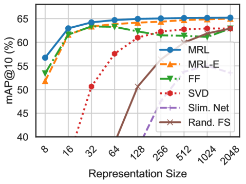
Figure 7: mAP@ $10$ for Image Retrieval on ImageNet-1K with ResNet50. ${\rm MRL}$ consistently produces better retrieval performance over the baselines across all the representation sizes.
Figure 7 compares the mAP@ $10$ performance of ResNet50 representations on ImageNet-1K across dimensionalities for ${\rm MRL}$ , ${\rm MRL\text{--}E}$ , FF, slimmable networks along with post-hoc compression of vectors using SVD and random feature selection. ${\rm Matryoshka~Representations}$ are often the most accurate while being up to $3\%$ better than the FF baselines. Similar to classification, post-hoc compression and slimmable network baselines suffer from significant drop-off in retrieval mAP@ $10$ with $≤ 256$ dimensions. Appendix E discusses the mAP@ $10$ of the same models on ImageNet-4K.
${\rm MRL}$ models are capable of performing accurate retrieval at various granularities without the additional expense of multiple model forward passes for the web-scale databases. FF models also generate independent databases which become prohibitively expense to store and switch in between. ${\rm Matryoshka~Representations}$ enable adaptive retrieval (AR) which alleviates the need to use full-capacity representations, $d=2048$ , for all data and downstream tasks. Lastly, all the vector compression techniques [60, 45] used as part of the ANNS pipelines are complimentary to ${\rm Matryoshka~Representations}$ and can further improve the efficiency-vs-accuracy trade-off.
4.3.1 Adaptive Retrieval
We benchmark ${\rm MRL}$ in the adaptive retrieval setting (AR) [50]. For a given query image, we obtained a shortlist, $K=200$ , of images from the database using a lower-dimensional representation, e.g. $D_{s}=16$ followed by reranking with a higher capacity representation, e.g. $D_{r}=2048$ . In real-world scenarios where top ranking performance is the key objective, measured with mAP@ $k$ where k covers a limited yet crucial real-estate, AR provides significant compute and memory gains over single-shot retrieval with representations of fixed dimensionality. Finally, the most expensive part of AR, as with any retrieval pipeline, is the nearest neighbour search for shortlisting. For example, even naive re-ranking of 200 images with 2048 dimensions only costs 400 KFLOPs. While we report exact search cost per query for all AR experiments, the shortlisting component of the pipeline can be sped-up using ANNS (HNSW). Appendix I has a detailed discussion on compute cost for exact search, memory overhead of HNSW indices and wall-clock times for both implementations. We note that using HNSW with 32 neighbours for shortlisting does not decrease accuracy during retrieval.
|
<details>
<summary>x15.png Details</summary>
### Visual Description
\n
## Scatter Plot: mAP@10 vs. MFLOPS/Query
### Overview
This scatter plot visualizes the relationship between mAP@10 (mean Average Precision at 10) and MFLOPS/Query (Millions of Floating Point Operations Per Second per Query). The plot includes two data series represented by different colored scatter points and trend lines, along with annotations indicating theoretical and real-world speed-up factors. A specific data point is highlighted with a "Funnel" label.
### Components/Axes
* **X-axis:** MFLOPS/Query, ranging from approximately 10^2 to 10^3 (logarithmic scale).
* **Y-axis:** mAP@10 (%), ranging from approximately 64.9 to 65.3.
* **Data Series 1 (Blue):** Represents "128x theoretical speed-up" with a dashed green line.
* **Data Series 2 (Orange):** Represents "14x real-world speed-up" with a dashed orange line.
* **Legend:** Located in the bottom-right corner, identifying the "Funnel" marker (orange 'Y' symbol).
* **Scatter Points:** Various shades of blue and purple, representing individual data points.
### Detailed Analysis
**X-axis:** The x-axis is labeled "MFLOPS/Query" and uses a logarithmic scale. The tick marks are at 10^2 and 10^3.
**Y-axis:** The y-axis is labeled "mAP@10 (%)" and ranges from 64.9 to 65.3, with gridlines at 0.1 intervals.
**Data Series 1 (Blue - 128x theoretical speed-up):**
The trend line slopes downward slightly.
* Approximately at MFLOPS/Query = 10^2, mAP@10 is approximately 65.25%.
* Approximately at MFLOPS/Query = 10^3, mAP@10 is approximately 65.2%.
**Data Series 2 (Orange - 14x real-world speed-up):**
The trend line slopes upward significantly.
* Approximately at MFLOPS/Query = 10^2, mAP@10 is approximately 64.95%.
* Approximately at MFLOPS/Query = 10^3, mAP@10 is approximately 65.2%.
**Scatter Points:**
* There are numerous scatter points distributed across the plot.
* The points generally cluster around the trend lines, but with considerable variance.
* A specific point is marked with an orange 'Y' symbol and labeled "Funnel". This point is located at approximately MFLOPS/Query = 10^2 and mAP@10 = 65.2.
### Key Observations
* The "real-world speed-up" (orange line) shows a more substantial increase in mAP@10 as MFLOPS/Query increases compared to the "theoretical speed-up" (green line).
* The theoretical speed-up line is relatively flat, suggesting diminishing returns in mAP@10 with increasing computational resources.
* The scatter points exhibit significant variability, indicating that factors beyond MFLOPS/Query influence mAP@10.
* The "Funnel" data point is located near the beginning of the x-axis and has a relatively high mAP@10 value.
### Interpretation
The plot demonstrates the trade-off between computational cost (MFLOPS/Query) and model performance (mAP@10). While theoretical speed-ups suggest limited gains, the real-world speed-up shows a more significant improvement in performance with increased computational resources. The scatter plot suggests that the relationship between these two variables is not strictly linear and is influenced by other factors. The "Funnel" data point may represent a specific model or configuration that achieves relatively high performance with lower computational cost. The difference between the theoretical and real-world speed-up lines highlights the importance of considering practical limitations and optimizations when evaluating model performance. The logarithmic scale on the x-axis suggests that the benefits of increasing MFLOPS/Query diminish as the value increases.
</details>
|
<details>
<summary>x16.png Details</summary>
### Visual Description
\n
## Heatmap: Ds vs Dr Correlation
### Overview
The image presents a heatmap-like visualization correlating two parameters, labeled *Ds* and *Dr*. The visualization uses a gradient of colors to represent values, with *Ds* values listed on the left and corresponding *Dr* values represented by the size and color of circles on the right. The image appears to demonstrate a relationship between these two parameters, where increasing *Ds* values correspond to increasing *Dr* values.
### Components/Axes
* **Vertical Axis (Ds):** Labeled "Ds", with values: 8, 16, 32, 64, 128, 256, 512, 1024, 2048.
* **Horizontal Axis (Dr):** Labeled "Dr", with no numerical values explicitly shown, but represented by the size and color of circles.
* **Color Gradient:** A gradient from light blue to dark purple, representing increasing values.
* **Circles:** Varying in size and color, representing the *Dr* value for each corresponding *Ds* value.
### Detailed Analysis
The visualization shows a clear correlation between *Ds* and *Dr*. As *Ds* increases, the size and intensity of the corresponding circle (representing *Dr*) also increases.
Here's a breakdown of the approximate *Dr* values based on the circle size and color:
* Ds = 8: Dr ≈ 1 (very small, light blue circle)
* Ds = 16: Dr ≈ 2 (small, light blue circle)
* Ds = 32: Dr ≈ 3 (slightly larger, light blue circle)
* Ds = 64: Dr ≈ 4 (medium, light blue circle)
* Ds = 128: Dr ≈ 7 (medium, purple circle)
* Ds = 256: Dr ≈ 10 (medium-large, purple circle)
* Ds = 512: Dr ≈ 15 (large, dark purple circle)
* Ds = 1024: Dr ≈ 20 (very large, dark purple circle)
* Ds = 2048: Dr ≈ 25 (largest, dark purple circle)
The color gradient progresses from light blue (low *Dr* values) to dark purple (high *Dr* values). The circles increase in diameter as *Ds* increases, visually representing the positive correlation.
### Key Observations
* The relationship between *Ds* and *Dr* appears to be non-linear. The increase in *Dr* seems to accelerate as *Ds* increases.
* The visualization provides a qualitative understanding of the relationship rather than precise numerical values for *Dr*.
* The scale for *Dr* is not explicitly defined, making it difficult to determine the exact units or range.
### Interpretation
This visualization likely represents a relationship between two parameters in a system where increasing *Ds* leads to a more significant effect, measured by *Dr*. The non-linear relationship suggests that the effect of *Ds* on *Dr* is not constant; it becomes more pronounced at higher values of *Ds*.
Without knowing the context of *Ds* and *Dr*, it's difficult to provide a more specific interpretation. However, the visualization suggests a positive feedback loop or an exponential relationship between the two parameters. The visualization is a qualitative representation of a correlation, and further analysis with precise numerical data would be needed to confirm the nature of the relationship and its underlying mechanisms.
</details>
|
<details>
<summary>x17.png Details</summary>
### Visual Description
## Scatter Plot: Performance Comparison
### Overview
This image presents a scatter plot comparing the performance of a system, likely a model or algorithm, across two metrics: MFLOPS/Query (on the x-axis, logarithmic scale) and mAP@10 (%) (on the y-axis). The plot shows a general trend of increasing mAP@10 with increasing MFLOPS/Query. Two specific points are highlighted with "Funnel" labels and connected by arrows indicating performance improvements. A dashed line represents a theoretical speed-up, and a dotted line represents a real-world speed-up.
### Components/Axes
* **X-axis:** MFLOPS/Query, ranging from 10<sup>2</sup> to 10<sup>4</sup> (logarithmic scale).
* **Y-axis:** mAP@10 (%), ranging from 16.0% to 17.5%.
* **Data Points:** Numerous circular data points, varying in size and color (primarily shades of blue and purple).
* **Legend:** Located in the bottom-right corner, containing a single entry:
* "Funnel" - Represented by a red inverted triangle symbol.
* **Annotations:**
* A green arrow pointing from a lighter blue point to a darker purple point, labeled "6x real-world speed-up".
* A dashed orange line connecting several purple points, labeled "32x theoretical speed-up".
* **Gridlines:** A gray grid is present to aid in reading values.
### Detailed Analysis
The plot contains a large number of data points, making precise extraction of all values difficult. However, key points and trends can be identified:
* **Funnel Point 1 (Left):** Located at approximately MFLOPS/Query = 200, mAP@10 = 16.2%. Marked with a red inverted triangle.
* **Funnel Point 2 (Right):** Located at approximately MFLOPS/Query = 8000, mAP@10 = 17.2%. Marked with a red inverted triangle.
* **Real-World Speed-Up Line:** This line starts around MFLOPS/Query = 200, mAP@10 = 16.2% and ends around MFLOPS/Query = 8000, mAP@10 = 17.2%. The line is relatively flat initially, then slopes upward.
* **Theoretical Speed-Up Line:** This line starts around MFLOPS/Query = 800, mAP@10 = 16.0% and ends around MFLOPS/Query = 4000, mAP@10 = 17.0%. This line shows a steeper upward slope than the real-world speed-up line.
* **Data Point Distribution:** The majority of data points are clustered in the lower-left region of the plot (low MFLOPS/Query, low mAP@10). There is a sparse scattering of points towards the upper-right (high MFLOPS/Query, high mAP@10).
* **Purple Points:** A cluster of purple points generally follow the trend of the "32x theoretical speed-up" line.
* **Blue Points:** The blue points are more dispersed and generally have lower mAP@10 values compared to the purple points.
### Key Observations
* There is a positive correlation between MFLOPS/Query and mAP@10. As computational throughput increases, the model's accuracy (as measured by mAP@10) also tends to increase.
* The "Funnel" points represent a significant performance improvement, with a 6x real-world speed-up observed.
* The theoretical speed-up (32x) is considerably higher than the real-world speed-up, suggesting limitations or bottlenecks in the actual implementation.
* The purple points, which follow the theoretical speed-up line, may represent optimized configurations or algorithms.
### Interpretation
The data suggests that increasing computational resources (MFLOPS/Query) can lead to improved model performance (mAP@10). However, the discrepancy between the theoretical and real-world speed-ups indicates that there are factors limiting the efficiency of the system. These factors could include memory bandwidth, communication overhead, or algorithmic inefficiencies. The "Funnel" points highlight a specific optimization or configuration that achieves a substantial performance gain. The scatter plot demonstrates the trade-off between computational cost and accuracy, and the potential for optimization to approach the theoretical limits of performance. The clustering of points suggests that certain regions of the parameter space are more favorable than others. The difference in distribution between the blue and purple points could indicate different model architectures or training strategies.
</details>
|
| --- | --- | --- |
| (a) ImageNet-1K | | (b) ImageNet-4K |
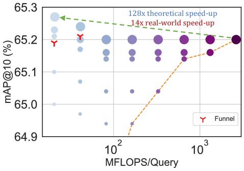
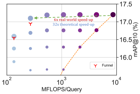
Figure 8: The trade-off between mAP@ $10$ vs MFLOPs/Query for Adaptive Retrieval (AR) on ImageNet-1K (left) and ImageNet-4K (right). Every combination of $D_{s}$ & $D_{r}$ falls above the Pareto line (orange dots) of single-shot retrieval with a fixed representation size while having configurations that are as accurate while being up to $14×$ faster in real-world deployment. Funnel retrieval is almost as accurate as the baseline while alleviating some of the parameter choices of Adaptive Retrieval.
Figure 8 showcases the compute-vs-accuracy trade-off for adaptive retrieval using ${\rm Matryoshka~Representations}$ compared to single-shot using fixed features with ResNet50 on ImageNet-1K. We observed that all AR settings lied above the Pareto frontier of single-shot retrieval with varying representation sizes. In particular for ImageNet-1K, we show that the AR model with $D_{s}=16$ & $D_{r}=2048$ is as accurate as single-shot retrieval with $d=2048$ while being $\mathbf{\sim 128×}$ more efficient in theory and $\mathbf{\sim 14×}$ faster in practice (compared using HNSW on the same hardware). We show similar trends with ImageNet-4K, but note that we require $D_{s}=64$ given the increased difficulty of the dataset. This results in $\sim 32×$ and $\sim 6×$ theoretical and in-practice speedups respectively. Lastly, while $K=200$ works well for our adaptive retrieval experiments, we ablated over the shortlist size $k$ in Appendix K.2 and found that the accuracy gains stopped after a point, further strengthening the use-case for ${\rm Matryoshka~Representation~Learning}$ and adaptive retrieval.
Even with adaptive retrieval, it is hard to determine the choice of $D_{s}$ & $D_{r}$ . In order to alleviate this issue to an extent, we propose Funnel Retrieval, a consistent cascade for adaptive retrieval. Funnel thins out the initial shortlist by a repeated re-ranking and shortlisting with a series of increasing capacity representations. Funnel halves the shortlist size and doubles the representation size at every step of re-ranking. For example on ImageNet-1K, a funnel with the shortlist progression of $200→ 100→ 50→ 25→ 10$ with the cascade of $16→ 32→ 64→ 128→ 256→ 2048$ representation sizes within ${\rm Matryoshka~Representation}$ is as accurate as the single-shot 2048-dim retrieval while being $\sim 128×$ more efficient theoretically (see Appendix F for more results). All these results showcase the potential of ${\rm MRL}$ and AR for large-scale multi-stage search systems [15].
5 Further Analysis and Ablations
Robustness.
We evaluate the robustness of the ${\rm MRL}$ models trained on ImageNet-1K on out-of-domain datasets, ImageNetV2/R/A/Sketch [72, 34, 35, 94], and compare them to the FF baselines. Table 17 in Appendix H demonstrates that ${\rm Matryoshka~Representations}$ for classification are at least as robust as the original representation while improving the performance on ImageNet-A by $0.6\%$ – a $20\%$ relative improvement. We also study the robustness in the context of retrieval by using ImageNetV2 as the query set for ImageNet-1K database. Table 9 in Appendix E shows that ${\rm MRL}$ models have more robust retrieval compared to the FF baselines by having up to $3\%$ higher mAP@ $10$ performance. This observation also suggests the need for further investigation into robustness using nearest neighbour based classification and retrieval instead of the standard linear probing setup. We also find that the zero-shot robustness of ALIGN- ${\rm MRL}$ (Table 18 in Appendix H) agrees with the observations made by Wortsman et al. [96]. Lastly, Table 6 in Appendix D.2 shows that ${\rm MRL}$ also improves the cosine similarity span between positive and random image-text pairs.
Few-shot and Long-tail Learning.
We exhaustively evaluated few-shot learning on ${\rm MRL}$ models using nearest class mean [79]. Table 15 in Appendix G shows that that representations learned through ${\rm MRL}$ perform comparably to FF representations across varying shots and number of classes.
${\rm Matryoshka~Representations}$ realize a unique pattern while evaluating on FLUID [92], a long-tail sequential learning framework. We observed that ${\rm MRL}$ provides up to $2\%$ accuracy higher on novel classes in the tail of the distribution, without sacrificing accuracy on other classes (Table 16 in Appendix G). Additionally we find the accuracy between low-dimensional and high-dimensional representations is marginal for pretrain classes. We hypothesize that the higher-dimensional representations are required to differentiate the classes when few training examples of each are known. This results provides further evidence that different tasks require varying capacity based on their difficulty.
| (a) (b) (c) |
<details>
<summary>TabsNFigs/images/gradcam-annotated-1.png Details</summary>

### Visual Description
\n
## Image Analysis: Visual Attention Heatmaps
### Overview
The image presents a series of heatmaps overlaid on a photograph of two people walking. The heatmaps visualize attention, likely from an AI model, as the complexity of the object being identified increases. The ground truth (GT) object is identified as a "Plastic Bag", and the heatmaps show the model's attention shifting from a "Shower Cap" to a "Plastic Bag" as the complexity increases. The complexity is indicated by numbers below each heatmap (8, 16, 32, 2048).
### Components/Axes
* **Image:** A photograph of two people walking on a street. The person on the left is wearing a dark coat and carrying a white plastic bag. The person on the right is wearing a blue jacket and carrying a red bag.
* **Heatmaps:** Five heatmaps are overlaid on the image, each representing a different level of complexity. The heatmaps use a color gradient, with purple indicating low attention and yellow indicating high attention.
* **Labels:**
* "GT: Plastic Bag" - Located at the top-left corner, indicating the ground truth object.
* "Shower Cap" - Label above the first heatmap.
* "Plastic Bag" - Label above the last heatmap.
* Arrow - A double-headed arrow pointing from "Shower Cap" to "Plastic Bag", indicating the shift in attention.
* Numerical values: 8, 16, 32, 2048 - Located below each heatmap, representing the complexity level.
### Detailed Analysis
The heatmaps show a clear shift in attention.
* **8 (First Heatmap):** The heatmap focuses primarily on the head of the person on the left, highlighting what the model initially identifies as a "Shower Cap". The attention is concentrated on the head region.
* **16 (Second Heatmap):** The attention begins to shift downwards, with some focus still on the head, but increasing attention on the white bag.
* **32 (Third Heatmap):** The attention continues to shift downwards, with the majority of the attention now focused on the white bag.
* **2048 (Fourth Heatmap):** The attention is almost entirely focused on the white bag, correctly identifying it as a "Plastic Bag". The heatmap shows a strong concentration of attention on the bag's shape and form.
The intensity of the yellow color (indicating high attention) increases as the complexity number increases, suggesting a more confident identification of the "Plastic Bag".
### Key Observations
* The model initially misidentifies the plastic bag as a shower cap at low complexity (8).
* As complexity increases, the model's attention shifts from the head to the bag.
* At high complexity (2048), the model accurately identifies the bag with strong confidence.
* The heatmaps demonstrate how increasing complexity can help an AI model refine its object recognition.
### Interpretation
This image demonstrates the process of object recognition refinement in an AI model. The initial misidentification of the plastic bag as a shower cap highlights the challenges of visual perception, especially with ambiguous shapes. The increasing complexity levels likely represent more processing power or more sophisticated algorithms being applied to the image. As the model processes more information (higher complexity), it is able to overcome the initial ambiguity and correctly identify the object. The shift in attention, visualized by the heatmaps, shows how the model learns to focus on the relevant features of the object. This is a common technique used in computer vision to understand how AI models "see" and interpret images. The arrow indicates a progression of understanding, from an initial incorrect assumption to a final correct identification. The data suggests that the model relies on contextual information and increasing processing power to resolve ambiguity and achieve accurate object recognition.
</details>
<details>
<summary>TabsNFigs/images/gradcam-annotated-2.png Details</summary>
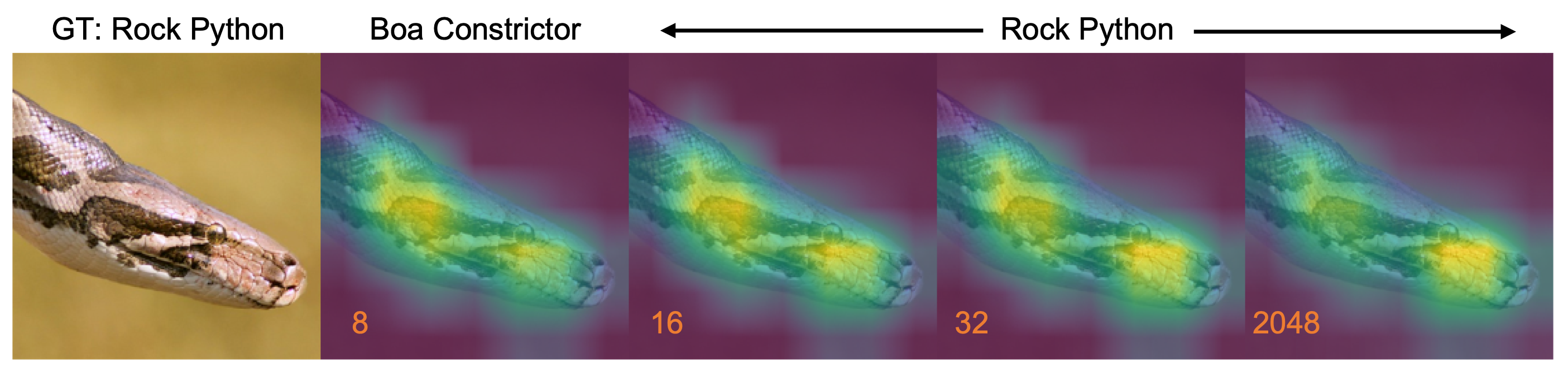
### Visual Description
\n
## Image: Snake Image Series with Numerical Labels
### Overview
The image presents a series of five images depicting snake heads, transitioning from a clear image of a Rock Python head on the left to progressively more blurred or abstracted images. Each image is accompanied by a numerical label positioned below it. A horizontal arrow spans the middle three images, labeled "Boa Constrictor" on the left and "Rock Python" on the right. The top-left corner is labeled "GT: Rock Python".
### Components/Axes
* **Labels:** "GT: Rock Python", "Boa Constrictor", "Rock Python", "8", "16", "32", "2048".
* **Images:** Five snake head images, visually decreasing in clarity from left to right.
* **Arrow:** A horizontal arrow pointing from left to right, spanning the middle three images.
### Detailed Analysis or Content Details
The image sequence can be broken down as follows:
1. **Image 1:** A clear, detailed image of a snake head, labeled "GT: Rock Python" in the top-left corner and "8" below.
2. **Image 2:** A slightly blurred image of a snake head, labeled "16" below.
3. **Image 3:** A more blurred image of a snake head, labeled "32" below.
4. **Image 4:** A significantly blurred image of a snake head, labeled "2048" below.
5. **Image 5:** A highly blurred image of a snake head.
The numerical labels (8, 16, 32, 2048) appear to be increasing, potentially representing a scale or parameter related to the image processing or abstraction. The arrow indicates a transition or comparison between "Boa Constrictor" and "Rock Python" as the images become more abstract.
### Key Observations
* The image clarity decreases as the numerical label increases.
* The initial image is explicitly identified as a "Rock Python".
* The arrow suggests a comparison or transformation between Boa Constrictor and Rock Python.
* The numerical values (8, 16, 32, 2048) form a geometric progression (doubling).
### Interpretation
The image likely demonstrates a process of image abstraction or compression. The "GT: Rock Python" label suggests a ground truth image, and the subsequent images show increasing levels of abstraction, potentially representing different compression ratios or levels of noise. The numerical labels likely correspond to these levels. The arrow and labels "Boa Constrictor" and "Rock Python" suggest that the process is being applied to both types of snakes, potentially to evaluate the robustness of a feature extraction or classification algorithm. The increasing numerical values (8, 16, 32, 2048) could represent the number of features used, the level of downsampling, or a similar parameter controlling the abstraction process. The image could be used to illustrate the trade-off between image clarity and computational efficiency in image processing or machine learning applications. The image does not provide any factual data beyond the labels and visual representation of the abstraction process.
</details>
<details>
<summary>TabsNFigs/images/gradcam-annotated-3.png Details</summary>
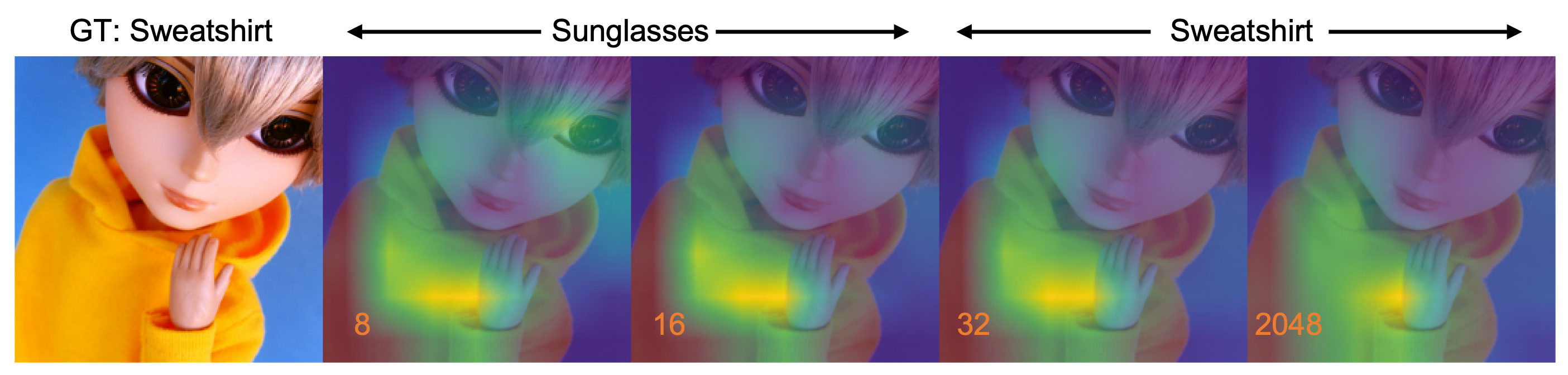
### Visual Description
\n
## Image: Visual Progression of Image Manipulation
### Overview
The image presents a series of four progressively altered images of a person wearing a yellow sweatshirt. The alterations appear to introduce the visual effect of sunglasses, with the intensity of the effect increasing from left to right. Numerical values are displayed below each image, likely representing a parameter controlling the strength or complexity of the effect. The image is framed by text indicating the "Ground Truth" (GT) is a sweatshirt and arrows indicating the direction of the manipulation towards sunglasses and back to a sweatshirt.
### Components/Axes
* **GT:** "Sweatshirt" - Located at the top-left corner, indicating the original image content.
* **Arrows:** Two bidirectional arrows labeled "Sunglasses" and "Sweatshirt" spanning the image horizontally, indicating the direction of the visual transformation.
* **Images:** Four images arranged horizontally, showing the progression of the effect.
* **Numerical Labels:** Four numerical labels ("8", "16", "32", "2048") positioned below each image, likely representing a parameter value.
### Detailed Analysis or Content Details
The images show a clear progression:
1. **Image 1 (Leftmost):** Shows a person wearing a bright yellow sweatshirt. No sunglasses effect is visible. Label: "8".
2. **Image 2:** Shows a subtle visual effect resembling a faint reflection or distortion on the eyes and face, suggesting the beginning of a sunglasses effect. The color palette shifts towards greens and blues. Label: "16".
3. **Image 3:** The sunglasses effect is more pronounced, with a more defined distortion around the eyes. The color palette continues to shift towards greens and blues, becoming more concentrated around the eye area. Label: "32".
4. **Image 4 (Rightmost):** The sunglasses effect is the most prominent, with a strong distortion around the eyes and a significant color shift. The color palette is dominated by greens and blues, with a concentrated effect around the eye area. Label: "2048".
The numerical labels increase exponentially (8, 16, 32, 2048), suggesting that the parameter they represent has a multiplicative or exponential effect on the visual transformation.
### Key Observations
* The visual effect appears to be an attempt to simulate the appearance of sunglasses being added to the image.
* The color palette changes significantly as the effect intensifies, shifting from the original yellow of the sweatshirt to a predominantly green and blue hue.
* The numerical labels suggest a parameter controlling the strength or complexity of the effect, with higher values resulting in a more pronounced transformation.
* The arrows indicate a transformation from the original "Sweatshirt" image towards the "Sunglasses" effect, and potentially back towards a modified "Sweatshirt" appearance.
### Interpretation
This image likely demonstrates a visual manipulation technique, possibly related to image editing or generative modeling. The progression of images suggests an algorithm or process that can transform an image from one state (sweatshirt) to another (sunglasses) by adjusting a specific parameter. The exponential increase in the parameter values (8, 16, 32, 2048) suggests that the effect is not linear, and that small changes in the parameter can lead to significant visual differences. The color changes may indicate the algorithm's method of simulating the light refraction or reflection caused by sunglasses. The image serves as a visual illustration of the impact of parameter tuning on the outcome of an image manipulation process. It could be used to demonstrate the capabilities of an image editing tool, or to visualize the inner workings of a generative model.
</details>
|
| --- | --- |
Figure 9: Grad-CAM [80] progression of predictions in ${\rm MRL}$ model across $8,16,32\text{ and }2048$ dimensions. (a) $8$ -dimensional representation confuses due to presence of other relevant objects (with a larger field of view) in the scene and predicts “shower cap” ; (b) $8$ -dim model confuses within the same super-class of “boa” ; (c) $8$ and $16$ -dim models incorrectly focus on the eyes of the doll ("sunglasses") and not the "sweatshirt" which is correctly in focus at higher dimensions; ${\rm MRL}$ fails gracefully in these scenarios and shows potential use cases of disagreement across dimensions.
Disagreement across Dimensions.
The information packing in ${\rm Matryoshka~Representations}$ often results in gradual increase of accuracy with increase in capacity. However, we observed that this trend was not ubiquitous and certain instances and classes were more accurate when evaluated with lower-dimensions (Figure 12 in Appendix J). With perfect routing of instances to appropriate dimension, ${\rm MRL}$ can gain up to $4.6\%$ classification accuracy. At the same time, the low-dimensional models are less accurate either due to confusion within the same superclass [24] of the ImageNet hierarchy or presence of multiple objects of interest. Figure 9 showcases 2 such examples for $8$ -dimensional representation. These results along with Appendix J put forward the potential for ${\rm MRL}$ to be a systematic framework for analyzing the utility and efficiency of information bottlenecks.
<details>
<summary>x18.png Details</summary>
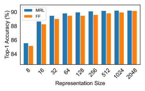
### Visual Description
\n
## Bar Chart: Top-1 Accuracy vs. Representation Size
### Overview
This bar chart compares the Top-1 Accuracy of two models, MRL and FF, across varying Representation Sizes. The chart uses bar graphs to display the accuracy values for each model at each representation size.
### Components/Axes
* **X-axis:** Representation Size. Values are: 8, 16, 32, 64, 128, 256, 512, 1024, 2048.
* **Y-axis:** Top-1 Accuracy (%). Scale ranges from approximately 83% to 91%.
* **Legend:**
* MRL (Blue)
* FF (Orange)
### Detailed Analysis
The chart consists of paired bars for each representation size, representing the Top-1 Accuracy of MRL and FF.
* **Representation Size 8:** MRL ≈ 85.5%, FF ≈ 84.5%
* **Representation Size 16:** MRL ≈ 88.3%, FF ≈ 88.3%
* **Representation Size 32:** MRL ≈ 89.3%, FF ≈ 88.7%
* **Representation Size 64:** MRL ≈ 89.7%, FF ≈ 89.3%
* **Representation Size 128:** MRL ≈ 89.8%, FF ≈ 89.7%
* **Representation Size 256:** MRL ≈ 89.9%, FF ≈ 89.8%
* **Representation Size 512:** MRL ≈ 90.1%, FF ≈ 89.9%
* **Representation Size 1024:** MRL ≈ 90.3%, FF ≈ 90.1%
* **Representation Size 2048:** MRL ≈ 90.4%, FF ≈ 90.3%
**Trends:**
* **MRL:** The blue bars (MRL) generally show an upward trend, increasing in height as the Representation Size increases. The increase appears to plateau after a Representation Size of 1024.
* **FF:** The orange bars (FF) also show an upward trend, similar to MRL, but consistently remain slightly below MRL's accuracy values. The increase also plateaus after a Representation Size of 1024.
### Key Observations
* MRL consistently outperforms FF across all Representation Sizes.
* The difference in accuracy between MRL and FF is relatively small, especially at larger Representation Sizes.
* Both models exhibit diminishing returns in accuracy as the Representation Size increases beyond 1024.
### Interpretation
The data suggests that increasing the Representation Size generally improves the Top-1 Accuracy of both the MRL and FF models. However, the improvement becomes marginal at larger Representation Sizes, indicating a point of diminishing returns. MRL consistently demonstrates slightly higher accuracy than FF, suggesting it may be a more effective model for this task, or that it benefits more from increased representation size. The plateauing of accuracy suggests that other factors, beyond Representation Size, may be limiting the performance of both models. This could include the quality of the training data, the model architecture, or the optimization algorithm used. Further investigation would be needed to determine the optimal Representation Size and identify other potential areas for improvement.
</details>
Figure 10: 31-way ImageNet-1K superclass classification across representation size for ${\rm MRL}$ & FF models showing the capture of underlying hierarchy through tight information bottlenecks.
<details>
<summary>x19.png Details</summary>
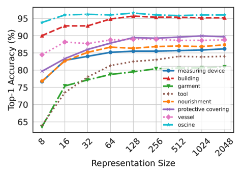
### Visual Description
## Line Chart: Top-1 Accuracy vs. Representation Size
### Overview
This line chart depicts the relationship between "Representation Size" and "Top-1 Accuracy" for several categories. The chart shows how the accuracy of identifying different object categories improves as the representation size increases. The chart has a grid background and a legend in the bottom-right corner.
### Components/Axes
* **X-axis:** "Representation Size" with values: 8, 16, 32, 64, 128, 256, 512, 1024, 2048.
* **Y-axis:** "Top-1 Accuracy (%)" with a scale ranging from approximately 65% to 96%.
* **Legend:** Located in the bottom-right corner, listing the following categories with corresponding colors:
* Measuring device (Green)
* Building (Red)
* Garment (Orange)
* Tool (Brown/Dashed)
* Nourishment (Blue)
* Protective covering (Purple)
* Vessel (Cyan/Dashed)
* Oscine (Teal)
### Detailed Analysis
Here's a breakdown of each line's trend and approximate data points, verified against the legend colors:
* **Measuring device (Green):** The line starts at approximately 66% accuracy at a representation size of 8, and increases rapidly to around 82% at a representation size of 32. It continues to increase, reaching approximately 92% at a representation size of 128, and plateaus around 93-94% for larger representation sizes.
* **Building (Red):** This line starts at approximately 77% accuracy at a representation size of 8, and increases steadily to around 93% at a representation size of 64. It then plateaus, remaining around 94-95% for larger representation sizes.
* **Garment (Orange):** The line begins at approximately 79% accuracy at a representation size of 8, and increases to around 88% at a representation size of 64. It continues to increase, reaching approximately 91% at a representation size of 256, and plateaus around 91-92% for larger representation sizes.
* **Tool (Brown/Dashed):** This line starts at approximately 72% accuracy at a representation size of 8, and increases gradually to around 80% at a representation size of 64. It continues to increase, reaching approximately 86% at a representation size of 512, and plateaus around 86-87% for larger representation sizes.
* **Nourishment (Blue):** The line starts at approximately 82% accuracy at a representation size of 8, and increases to around 86% at a representation size of 64. It then plateaus, remaining around 86-87% for larger representation sizes.
* **Protective covering (Purple):** This line starts at approximately 75% accuracy at a representation size of 8, and increases to around 88% at a representation size of 128. It continues to increase, reaching approximately 90% at a representation size of 256, and plateaus around 90-91% for larger representation sizes.
* **Vessel (Cyan/Dashed):** The line begins at approximately 80% accuracy at a representation size of 8, and increases to around 88% at a representation size of 64. It continues to increase, reaching approximately 90% at a representation size of 256, and plateaus around 90-91% for larger representation sizes.
* **Oscine (Teal):** The line starts at approximately 74% accuracy at a representation size of 8, and increases to around 84% at a representation size of 128. It continues to increase, reaching approximately 89% at a representation size of 512, and plateaus around 89-90% for larger representation sizes.
### Key Observations
* The "Building" category consistently exhibits the highest accuracy across all representation sizes.
* The "Measuring device" category shows the most significant improvement in accuracy with increasing representation size, particularly between 8 and 128.
* The accuracy of most categories plateaus after a representation size of 256, indicating diminishing returns from further increasing the representation size.
* The "Tool" and "Oscine" categories have the lowest overall accuracy compared to the other categories.
### Interpretation
The data suggests that increasing the representation size generally improves the accuracy of identifying these object categories. However, the rate of improvement diminishes as the representation size increases, and there is a point of diminishing returns. The varying accuracy levels across categories indicate that some objects are inherently easier to identify than others, potentially due to their visual distinctiveness or the quality of the training data. The plateauing effect suggests that the model has reached its capacity to extract useful information from the representation for these specific categories. This information could be used to optimize model training and resource allocation, focusing on categories with lower accuracy or exploring alternative representation techniques. The dashed lines for "Tool" and "Vessel" may indicate a different training methodology or data source compared to the solid lines.
</details>
Figure 11: Diverse per-superclass accuracy trends across representation sizes for ResNet50- ${\rm MRL}$ on ImageNet-1K.
Superclass Accuracy.
As the information bottleneck becomes smaller, the overall accuracy on fine-grained classes decreases rapidly (Figure 3). However, the drop-off is not as significant when evaluated at a superclass level (Table 24 in Appendix J). Figure 11 presents that this phenomenon occurs with both ${\rm MRL}$ and FF models; ${\rm MRL}$ is more accurate across dimensions. This shows that tight information bottlenecks while not highly accurate for fine-grained classification, do capture required semantic information for coarser classification that could be leveraged for adaptive routing for retrieval and classification. Mutifidelity of ${\rm Matryoshka~Representation}$ naturally captures the underlying hierarchy of the class labels with one single model. Lastly, Figure 11 showcases the accuracy trends per superclass with ${\rm MRL}$ . The utility of additional dimensions in distinguishing a class from others within the same superclass is evident for “garment” which has up to 11% improvement for 8 $→$ 16 dimensional representation transition. We also observed that superclasses such as “oscine (songbird)” had a clear visual distinction between the object and background and thus predictions using 8 dimensions also led to a good inter-class separability within the superclass.
5.1 Ablations
Table 26 in Appendix K presents that ${\rm Matryoshka~Representations}$ can be enabled within off-the-shelf pretrained models with inexpensive partial finetuning thus paving a way for ubiquitous adoption of ${\rm MRL}$ . At the same time, Table 27 in Appendix C indicates that with optimal weighting of the nested losses we could improve accuracy of lower-dimensions representations without accuracy loss. Tables 29 and 29 in Appendix C ablate over the choice of initial granularity and spacing of the granularites. Table 29 reaffirms the design choice to shun extremely low dimensions that have poor classification accuracy as initial granularity for ${\rm MRL}$ while Table 29 confirms the effectiveness of logarthmic granularity spacing inspired from the behaviour of accuracy saturation across dimensions over uniform. Lastly, Tables 30 and 31 in Appendix K.2 show that the retrieval performance saturates after a certain shortlist dimension and length depending on the complexity of the dataset.
6 Discussion and Conclusions
The results in Section 5.1 reveal interesting weaknesses of ${\rm MRL}$ that would be logical directions for future work. (1) Optimizing the weightings of the nested losses to obtain a Pareto optimal accuracy-vs-efficiency trade-off – a potential solution could emerge from adaptive loss balancing aspects of anytime neural networks [41]. (2) Using different losses at various fidelities aimed at solving a specific aspect of adaptive deployment – e.g. high recall for $8$ -dimension and robustness for $2048$ -dimension. (3) Learning a search data-structure, like differentiable k-d tree, on top of ${\rm Matryoshka~Representation}$ to enable dataset and representation aware retrieval. (4) Finally, the joint optimization of multi-objective ${\rm MRL}$ combined with end-to-end learnable search data-structure to have data-driven adaptive large-scale retrieval for web-scale search applications.
In conclusion, we presented
<details>
<summary>x20.png Details</summary>

### Visual Description
Icon/Small Image (28x28)
</details>
${\rm Matryoshka~Representation~Learning}$ ( ${\rm MRL}$ ), a flexible representation learning approach that encodes information at multiple granularities in a single embedding vector. This enables the ${\rm MRL}$ to adapt to a downstream task’s statistical complexity as well as the available compute resources. We demonstrate that ${\rm MRL}$ can be used for large-scale adaptive classification as well as adaptive retrieval. On standard benchmarks, ${\rm MRL}$ matches the accuracy of the fixed-feature baseline despite using $14×$ smaller representation size on average. Furthermore, the ${\rm Matryoshka~Representation}$ based adaptive shortlisting and re-ranking system ensures comparable mAP@ $10$ to the baseline while being $128×$ cheaper in FLOPs and $14×$ faster in wall-clock time. Finally, most of the efficiency techniques for model inference and vector search are complementary to ${\rm MRL}$
<details>
<summary>x21.png Details</summary>

### Visual Description
Icon/Small Image (28x28)
</details>
further assisting in deployment at the compute-extreme environments.
Acknowledgments
We are grateful to Srinadh Bhojanapalli, Lovish Madaan, Raghav Somani, Ludwig Schmidt, and Venkata Sailesh Sanampudi for helpful discussions and feedback. Aditya Kusupati also thanks Tom Duerig and Rahul Sukthankar for their support. Part of the paper’s large-scale experimentation is supported through a research GCP credit award from Google Cloud and Google Research. Gantavya Bhatt is supported in part by the CONIX Research Center, one of six centers in JUMP, a Semiconductor Research Corporation (SRC) program sponsored by DARPA. Sham Kakade acknowledges funding from the NSF award CCF-1703574 and ONR N00014-22-1-2377. Ali Farhadi acknowledges funding from the NSF awards IIS 1652052, IIS 17303166, DARPA N66001-19-2-4031, DARPA W911NF-15-1-0543 and gifts from Allen Institute for Artificial Intelligence.
References
- Abadi et al. [2015] M. Abadi, A. Agarwal, P. Barham, E. Brevdo, Z. Chen, C. Citro, G. S. Corrado, A. Davis, J. Dean, M. Devin, S. Ghemawat, I. Goodfellow, A. Harp, G. Irving, M. Isard, Y. Jia, R. Jozefowicz, L. Kaiser, M. Kudlur, J. Levenberg, D. Mané, R. Monga, S. Moore, D. Murray, C. Olah, M. Schuster, J. Shlens, B. Steiner, I. Sutskever, K. Talwar, P. Tucker, V. Vanhoucke, V. Vasudevan, F. Viégas, O. Vinyals, P. Warden, M. Wattenberg, M. Wicke, Y. Yu, and X. Zheng. TensorFlow: Large-scale machine learning on heterogeneous systems, 2015. URL https://www.tensorflow.org/. Software available from tensorflow.org.
- Barbu et al. [2019] A. Barbu, D. Mayo, J. Alverio, W. Luo, C. Wang, D. Gutfreund, J. Tenenbaum, and B. Katz. Objectnet: A large-scale bias-controlled dataset for pushing the limits of object recognition models. Advances in neural information processing systems, 32, 2019.
- Bengio et al. [2010] S. Bengio, J. Weston, and D. Grangier. Label embedding trees for large multi-class tasks. Advances in Neural Information Processing Systems, 23, 2010.
- Bengio [2012] Y. Bengio. Deep learning of representations for unsupervised and transfer learning. In Proceedings of ICML workshop on unsupervised and transfer learning, pages 17–36. JMLR Workshop and Conference Proceedings, 2012.
- Bentley [1990] J. L. Bentley. K-d trees for semidynamic point sets. In Proceedings of the sixth annual symposium on Computational geometry, pages 187–197, 1990.
- Beygelzimer et al. [2006] A. Beygelzimer, S. Kakade, and J. Langford. Cover trees for nearest neighbor. In Proceedings of the 23rd international conference on Machine learning, pages 97–104, 2006.
- Brin and Page [1998] S. Brin and L. Page. The anatomy of a large-scale hypertextual web search engine. Computer networks and ISDN systems, 30(1-7):107–117, 1998.
- Brown et al. [2020] T. Brown, B. Mann, N. Ryder, M. Subbiah, J. D. Kaplan, P. Dhariwal, A. Neelakantan, P. Shyam, G. Sastry, A. Askell, et al. Language models are few-shot learners. Advances in neural information processing systems, 33:1877–1901, 2020.
- Cai et al. [2019] H. Cai, C. Gan, T. Wang, Z. Zhang, and S. Han. Once-for-all: Train one network and specialize it for efficient deployment. arXiv preprint arXiv:1908.09791, 2019.
- Chang et al. [2020] W.-C. Chang, F. X. Yu, Y.-W. Chang, Y. Yang, and S. Kumar. Pre-training tasks for embedding-based large-scale retrieval. arXiv preprint arXiv:2002.03932, 2020.
- Chang et al. [2021] W.-C. Chang, D. Jiang, H.-F. Yu, C. H. Teo, J. Zhang, K. Zhong, K. Kolluri, Q. Hu, N. Shandilya, V. Ievgrafov, et al. Extreme multi-label learning for semantic matching in product search. In Proceedings of the 27th ACM SIGKDD Conference on Knowledge Discovery & Data Mining, pages 2643–2651, 2021.
- Chen et al. [2020] T. Chen, S. Kornblith, M. Norouzi, and G. Hinton. A simple framework for contrastive learning of visual representations. In International conference on machine learning, pages 1597–1607. PMLR, 2020.
- Chen et al. [2021] Y. Chen, Z. Liu, H. Xu, T. Darrell, and X. Wang. Meta-baseline: exploring simple meta-learning for few-shot learning. In Proceedings of the IEEE/CVF International Conference on Computer Vision, pages 9062–9071, 2021.
- Datar et al. [2004] M. Datar, N. Immorlica, P. Indyk, and V. S. Mirrokni. Locality-sensitive hashing scheme based on p-stable distributions. In Proceedings of the twentieth annual symposium on Computational geometry, pages 253–262, 2004.
- Dean [2009] J. Dean. Challenges in building large-scale information retrieval systems. In Keynote of the 2nd ACM International Conference on Web Search and Data Mining (WSDM), volume 10, 2009.
- Deng et al. [2009] J. Deng, W. Dong, R. Socher, L.-J. Li, K. Li, and L. Fei-Fei. Imagenet: A large-scale hierarchical image database. In 2009 IEEE conference on computer vision and pattern recognition, pages 248–255. Ieee, 2009.
- Deng et al. [2011] J. Deng, A. C. Berg, and L. Fei-Fei. Hierarchical semantic indexing for large scale image retrieval. In CVPR 2011, pages 785–792. IEEE, 2011.
- Desai and Johnson [2021] K. Desai and J. Johnson. Virtex: Learning visual representations from textual annotations. In Proceedings of the IEEE/CVF Conference on Computer Vision and Pattern Recognition, pages 11162–11173, 2021.
- Devlin et al. [2018] J. Devlin, M.-W. Chang, K. Lee, and K. Toutanova. Bert: Pre-training of deep bidirectional transformers for language understanding. arXiv preprint arXiv:1810.04805, 2018.
- Dietterich and Bakiri [1994] T. G. Dietterich and G. Bakiri. Solving multiclass learning problems via error-correcting output codes. Journal of artificial intelligence research, 2:263–286, 1994.
- Divvala et al. [2014] S. K. Divvala, A. Farhadi, and C. Guestrin. Learning everything about anything: Webly-supervised visual concept learning. In Proceedings of the IEEE Conference on Computer Vision and Pattern Recognition, pages 3270–3277, 2014.
- Dosovitskiy et al. [2020] A. Dosovitskiy, L. Beyer, A. Kolesnikov, D. Weissenborn, X. Zhai, T. Unterthiner, M. Dehghani, M. Minderer, G. Heigold, S. Gelly, et al. An image is worth 16x16 words: Transformers for image recognition at scale. arXiv preprint arXiv:2010.11929, 2020.
- Engelsma et al. [2022] J. J. Engelsma, A. K. Jain, and V. N. Boddeti. Hers: Homomorphically encrypted representation search. IEEE Transactions on Biometrics, Behavior, and Identity Science, 4(3):349–360, 2022.
- Engstrom et al. [2019] L. Engstrom, A. Ilyas, H. Salman, S. Santurkar, and D. Tsipras. Robustness (python library), 2019. URL https://github.com/MadryLab/robustness.
- Gholami et al. [2021] A. Gholami, S. Kim, Z. Dong, Z. Yao, M. W. Mahoney, and K. Keutzer. A survey of quantization methods for efficient neural network inference. arXiv preprint arXiv:2103.13630, 2021.
- Gong et al. [2019] S. Gong, V. N. Boddeti, and A. K. Jain. On the intrinsic dimensionality of image representations. In Proceedings of the IEEE/CVF Conference on Computer Vision and Pattern Recognition, pages 3987–3996, 2019.
- Gutmann and Hyvärinen [2010] M. Gutmann and A. Hyvärinen. Noise-contrastive estimation: A new estimation principle for unnormalized statistical models. In Proceedings of the thirteenth international conference on artificial intelligence and statistics, pages 297–304. JMLR Workshop and Conference Proceedings, 2010.
- Harris and Giachritsis [2000] M. G. Harris and C. D. Giachritsis. Coarse-grained information dominates fine-grained information in judgments of time-to-contact from retinal flow. Vision research, 40(6):601–611, 2000.
- He et al. [2016] K. He, X. Zhang, S. Ren, and J. Sun. Deep residual learning for image recognition. In Proceedings of the IEEE conference on computer vision and pattern recognition, pages 770–778, 2016.
- He et al. [2020] K. He, H. Fan, Y. Wu, S. Xie, and R. Girshick. Momentum contrast for unsupervised visual representation learning. In Proceedings of the IEEE/CVF conference on computer vision and pattern recognition, pages 9729–9738, 2020.
- He et al. [2021] K. He, X. Chen, S. Xie, Y. Li, P. Dollár, and R. Girshick. Masked autoencoders are scalable vision learners. arXiv preprint arXiv:2111.06377, 2021.
- Hegdé [2008] J. Hegdé. Time course of visual perception: coarse-to-fine processing and beyond. Progress in neurobiology, 84(4):405–439, 2008.
- Hendrycks and Gimpel [2016] D. Hendrycks and K. Gimpel. A baseline for detecting misclassified and out-of-distribution examples in neural networks. arXiv preprint arXiv:1610.02136, 2016.
- Hendrycks et al. [2021a] D. Hendrycks, S. Basart, N. Mu, S. Kadavath, F. Wang, E. Dorundo, R. Desai, T. Zhu, S. Parajuli, M. Guo, et al. The many faces of robustness: A critical analysis of out-of-distribution generalization. In Proceedings of the IEEE/CVF International Conference on Computer Vision, pages 8340–8349, 2021a.
- Hendrycks et al. [2021b] D. Hendrycks, K. Zhao, S. Basart, J. Steinhardt, and D. Song. Natural adversarial examples. In Proceedings of the IEEE/CVF Conference on Computer Vision and Pattern Recognition, pages 15262–15271, 2021b.
- Hooker et al. [2019] S. Hooker, A. Courville, G. Clark, Y. Dauphin, and A. Frome. What do compressed deep neural networks forget? arXiv preprint arXiv:1911.05248, 2019.
- Hooker et al. [2020] S. Hooker, N. Moorosi, G. Clark, S. Bengio, and E. Denton. Characterising bias in compressed models. arXiv preprint arXiv:2010.03058, 2020.
- Hotelling [1933] H. Hotelling. Analysis of a complex of statistical variables into principal components. Journal of educational psychology, 24(6):417, 1933.
- Howard et al. [2017] A. G. Howard, M. Zhu, B. Chen, D. Kalenichenko, W. Wang, T. Weyand, M. Andreetto, and H. Adam. Mobilenets: Efficient convolutional neural networks for mobile vision applications. arXiv preprint arXiv:1704.04861, 2017.
- Howard and Ruder [2018] J. Howard and S. Ruder. Universal language model fine-tuning for text classification. arXiv preprint arXiv:1801.06146, 2018.
- Hu et al. [2019] H. Hu, D. Dey, M. Hebert, and J. A. Bagnell. Learning anytime predictions in neural networks via adaptive loss balancing. In Proceedings of the AAAI Conference on Artificial Intelligence, volume 33, pages 3812–3821, 2019.
- Indyk and Motwani [1998] P. Indyk and R. Motwani. Approximate nearest neighbors: towards removing the curse of dimensionality. In Proceedings of the thirtieth annual ACM symposium on Theory of computing, pages 604–613, 1998.
- Jain et al. [2019] H. Jain, V. Balasubramanian, B. Chunduri, and M. Varma. Slice: Scalable linear extreme classifiers trained on 100 million labels for related searches. In Proceedings of the Twelfth ACM International Conference on Web Search and Data Mining, pages 528–536, 2019.
- Jayaram Subramanya et al. [2019] S. Jayaram Subramanya, F. Devvrit, H. V. Simhadri, R. Krishnawamy, and R. Kadekodi. Diskann: Fast accurate billion-point nearest neighbor search on a single node. Advances in Neural Information Processing Systems, 32, 2019.
- Jegou et al. [2010] H. Jegou, M. Douze, and C. Schmid. Product quantization for nearest neighbor search. IEEE transactions on pattern analysis and machine intelligence, 33(1):117–128, 2010.
- Jia et al. [2021] C. Jia, Y. Yang, Y. Xia, Y.-T. Chen, Z. Parekh, H. Pham, Q. Le, Y.-H. Sung, Z. Li, and T. Duerig. Scaling up visual and vision-language representation learning with noisy text supervision. In International Conference on Machine Learning, pages 4904–4916. PMLR, 2021.
- Johnson et al. [2019] J. Johnson, M. Douze, and H. Jégou. Billion-scale similarity search with GPUs. IEEE Transactions on Big Data, 7(3):535–547, 2019.
- Johnson [1984] W. B. Johnson. Extensions of lipschitz mappings into a hilbert space. Contemp. Math., 26:189–206, 1984.
- Jouppi et al. [2017] N. P. Jouppi, C. Young, N. Patil, D. Patterson, G. Agrawal, R. Bajwa, S. Bates, S. Bhatia, N. Boden, A. Borchers, et al. In-datacenter performance analysis of a tensor processing unit. In Proceedings of the 44th annual international symposium on computer architecture, pages 1–12, 2017.
- Kaz Sato [2021] T. C. Kaz Sato. Vertex ai matching engine. Microsoft AI Blog, 2021. URL https://cloud.google.com/blog/topics/developers-practitioners/find-anything-blazingly-fast-googles-vector-search-technology.
- Krizhevsky et al. [2012] A. Krizhevsky, I. Sutskever, and G. E. Hinton. Imagenet classification with deep convolutional neural networks. Advances in neural information processing systems, 25, 2012.
- Kulis et al. [2009] B. Kulis, P. Jain, and K. Grauman. Fast similarity search for learned metrics. IEEE Transactions on Pattern Analysis and Machine Intelligence, 31(12):2143–2157, 2009.
- Kusupati et al. [2018] A. Kusupati, M. Singh, K. Bhatia, A. Kumar, P. Jain, and M. Varma. Fastgrnn: A fast, accurate, stable and tiny kilobyte sized gated recurrent neural network. Advances in Neural Information Processing Systems, 31, 2018.
- Kusupati et al. [2020] A. Kusupati, V. Ramanujan, R. Somani, M. Wortsman, P. Jain, S. Kakade, and A. Farhadi. Soft threshold weight reparameterization for learnable sparsity. In International Conference on Machine Learning, pages 5544–5555. PMLR, 2020.
- Kusupati et al. [2021] A. Kusupati, M. Wallingford, V. Ramanujan, R. Somani, J. S. Park, K. Pillutla, P. Jain, S. Kakade, and A. Farhadi. Llc: Accurate, multi-purpose learnt low-dimensional binary codes. Advances in Neural Information Processing Systems, 34, 2021.
- Leclerc et al. [2022] G. Leclerc, A. Ilyas, L. Engstrom, S. M. Park, H. Salman, and A. Madry. ffcv. https://github.com/libffcv/ffcv/, 2022. commit 607d117.
- LeCun et al. [2015] Y. LeCun, Y. Bengio, and G. Hinton. Deep learning. nature, 521(7553):436–444, 2015.
- Lee et al. [2016] S. Lee, S. Purushwalkam Shiva Prakash, M. Cogswell, V. Ranjan, D. Crandall, and D. Batra. Stochastic multiple choice learning for training diverse deep ensembles. Advances in Neural Information Processing Systems, 29, 2016.
- Li et al. [2018] C. Li, H. Farkhoor, R. Liu, and J. Yosinski. Measuring the intrinsic dimension of objective landscapes. arXiv preprint arXiv:1804.08838, 2018.
- Linde et al. [1980] Y. Linde, A. Buzo, and R. Gray. An algorithm for vector quantizer design. IEEE Transactions on communications, 28(1):84–95, 1980.
- Loshchilov and Hutter [2017] I. Loshchilov and F. Hutter. Decoupled weight decay regularization. arXiv preprint arXiv:1711.05101, 2017.
- Malkov and Yashunin [2018] Y. A. Malkov and D. A. Yashunin. Efficient and robust approximate nearest neighbor search using hierarchical navigable small world graphs. IEEE transactions on pattern analysis and machine intelligence, 42(4):824–836, 2018.
- Masci et al. [2011] J. Masci, U. Meier, D. Cireşan, and J. Schmidhuber. Stacked convolutional auto-encoders for hierarchical feature extraction. In International conference on artificial neural networks, pages 52–59. Springer, 2011.
- Mitra et al. [2002] P. Mitra, C. Murthy, and S. K. Pal. Unsupervised feature selection using feature similarity. IEEE transactions on pattern analysis and machine intelligence, 24(3):301–312, 2002.
- Nanda et al. [2023] V. Nanda, T. Speicher, J. P. Dickerson, S. Feizi, K. P. Gummadi, and A. Weller. Diffused redundancy in pre-trained representations. arXiv preprint arXiv:2306.00183, 2023.
- Nayak [2019] P. Nayak. Understanding searches better than ever before. Google AI Blog, 2019. URL https://blog.google/products/search/search-language-understanding-bert/.
- Paszke et al. [2019] A. Paszke, S. Gross, F. Massa, A. Lerer, J. Bradbury, G. Chanan, T. Killeen, Z. Lin, N. Gimelshein, L. Antiga, et al. Pytorch: An imperative style, high-performance deep learning library. Advances in neural information processing systems, 32, 2019.
- Peters et al. [2018] M. E. Peters, M. Neumann, M. Iyyer, M. Gardner, C. Clark, K. Lee, and L. Zettlemoyer. Deep contextualized word representations. In Proceedings of the 2018 Conference of the North American Chapter of the Association for Computational Linguistics: Human Language Technologies, Volume 1 (Long Papers), pages 2227–2237, New Orleans, Louisiana, June 2018. Association for Computational Linguistics. doi: 10.18653/v1/N18-1202. URL https://aclanthology.org/N18-1202.
- Prabhu et al. [2020] Y. Prabhu, A. Kusupati, N. Gupta, and M. Varma. Extreme regression for dynamic search advertising. In Proceedings of the 13th International Conference on Web Search and Data Mining, pages 456–464, 2020.
- Radford et al. [2018] A. Radford, K. Narasimhan, T. Salimans, and I. Sutskever. Improving language understanding by generative pre-training. OpenAI Blog, 2018. URL https://openai.com/blog/language-unsupervised/.
- Radford et al. [2021] A. Radford, J. W. Kim, C. Hallacy, A. Ramesh, G. Goh, S. Agarwal, G. Sastry, A. Askell, P. Mishkin, J. Clark, et al. Learning transferable visual models from natural language supervision. In International Conference on Machine Learning, pages 8748–8763. PMLR, 2021.
- Recht et al. [2019] B. Recht, R. Roelofs, L. Schmidt, and V. Shankar. Do imagenet classifiers generalize to imagenet? In International Conference on Machine Learning, pages 5389–5400. PMLR, 2019.
- Rippel et al. [2014] O. Rippel, M. Gelbart, and R. Adams. Learning ordered representations with nested dropout. In International Conference on Machine Learning, pages 1746–1754. PMLR, 2014.
- Rissanen [1978] J. Rissanen. Modeling by shortest data description. Automatica, 14(5):465–471, 1978.
- Ruder et al. [2019] S. Ruder, M. E. Peters, S. Swayamdipta, and T. Wolf. Transfer learning in natural language processing. In Proceedings of the 2019 conference of the North American chapter of the association for computational linguistics: Tutorials, pages 15–18, 2019.
- Russakovsky et al. [2015] O. Russakovsky, J. Deng, H. Su, J. Krause, S. Satheesh, S. Ma, Z. Huang, A. Karpathy, A. Khosla, M. Bernstein, et al. Imagenet large scale visual recognition challenge. International journal of computer vision, 115(3):211–252, 2015.
- Salakhutdinov and Hinton [2007] R. Salakhutdinov and G. Hinton. Learning a nonlinear embedding by preserving class neighbourhood structure. In Artificial Intelligence and Statistics, pages 412–419. PMLR, 2007.
- Salakhutdinov and Hinton [2009] R. Salakhutdinov and G. Hinton. Semantic hashing. International Journal of Approximate Reasoning, 50(7):969–978, 2009.
- Sánchez et al. [1997] J. S. Sánchez, F. Pla, and F. J. Ferri. On the use of neighbourhood-based non-parametric classifiers. Pattern Recognition Letters, 18(11-13):1179–1186, 1997.
- Selvaraju et al. [2017] R. R. Selvaraju, M. Cogswell, A. Das, R. Vedantam, D. Parikh, and D. Batra. Grad-cam: Visual explanations from deep networks via gradient-based localization. In Proceedings of the IEEE international conference on computer vision, pages 618–626, 2017.
- Shazeer and Stern [2018] N. Shazeer and M. Stern. Adafactor: Adaptive learning rates with sublinear memory cost. In International Conference on Machine Learning, pages 4596–4604. PMLR, 2018.
- Simonyan and Zisserman [2014] K. Simonyan and A. Zisserman. Very deep convolutional networks for large-scale image recognition. arXiv preprint arXiv:1409.1556, 2014.
- Smith [2017] L. N. Smith. Cyclical learning rates for training neural networks. In 2017 IEEE winter conference on applications of computer vision (WACV), pages 464–472. IEEE, 2017.
- Soudry et al. [2018] D. Soudry, E. Hoffer, M. S. Nacson, S. Gunasekar, and N. Srebro. The implicit bias of gradient descent on separable data. The Journal of Machine Learning Research, 19(1):2822–2878, 2018.
- Sun et al. [2017] C. Sun, A. Shrivastava, S. Singh, and A. Gupta. Revisiting unreasonable effectiveness of data in deep learning era. In Proceedings of the IEEE international conference on computer vision, pages 843–852, 2017.
- Sutskever et al. [2013] I. Sutskever, J. Martens, G. Dahl, and G. Hinton. On the importance of initialization and momentum in deep learning. In International conference on machine learning, pages 1139–1147. PMLR, 2013.
- Tan and Le [2019] M. Tan and Q. Le. Efficientnet: Rethinking model scaling for convolutional neural networks. In International conference on machine learning, pages 6105–6114. PMLR, 2019.
- Van Der Maaten et al. [2009] L. Van Der Maaten, E. Postma, J. Van den Herik, et al. Dimensionality reduction: a comparative. J Mach Learn Res, 10(66-71):13, 2009.
- Varma [2019] M. Varma. Extreme classification. Communications of the ACM, 62(11):44–45, 2019.
- Viola and Jones [2001] P. Viola and M. Jones. Rapid object detection using a boosted cascade of simple features. In Proceedings of the 2001 IEEE computer society conference on computer vision and pattern recognition. CVPR 2001, volume 1, pages I–I. Ieee, 2001.
- Waldburger [2019] C. Waldburger. As search needs evolve, microsoft makes ai tools for better search available to researchers and developers. Microsoft AI Blog, 2019. URL https://blogs.microsoft.com/ai/bing-vector-search/.
- Wallingford et al. [2020] M. Wallingford, A. Kusupati, K. Alizadeh-Vahid, A. Walsman, A. Kembhavi, and A. Farhadi. Are we overfitting to experimental setups in recognition? arXiv preprint arXiv:2007.02519, 2020.
- Wallingford et al. [2022] M. Wallingford, H. Li, A. Achille, A. Ravichandran, C. Fowlkes, R. Bhotika, and S. Soatto. Task adaptive parameter sharing for multi-task learning. arXiv preprint arXiv:2203.16708, 2022.
- Wang et al. [2019] H. Wang, S. Ge, Z. Lipton, and E. P. Xing. Learning robust global representations by penalizing local predictive power. In Advances in Neural Information Processing Systems, pages 10506–10518, 2019.
- Wang et al. [2020] X. Wang, D. Kondratyuk, K. M. Kitani, Y. Movshovitz-Attias, and E. Eban. Multiple networks are more efficient than one: Fast and accurate models via ensembles and cascades. arXiv preprint arXiv:2012.01988, 2020.
- Wortsman et al. [2021] M. Wortsman, G. Ilharco, M. Li, J. W. Kim, H. Hajishirzi, A. Farhadi, H. Namkoong, and L. Schmidt. Robust fine-tuning of zero-shot models. arXiv preprint arXiv:2109.01903, 2021.
- Wu et al. [2018] Z. Wu, Y. Xiong, S. Yu, and D. Lin. Unsupervised feature learning via non-parametric instance-level discrimination. arXiv preprint arXiv:1805.01978, 2018.
- Yosinski et al. [2014] J. Yosinski, J. Clune, Y. Bengio, and H. Lipson. How transferable are features in deep neural networks? Advances in neural information processing systems, 27, 2014.
- Yu et al. [2022] H.-F. Yu, K. Zhong, J. Zhang, W.-C. Chang, and I. S. Dhillon. Pecos: Prediction for enormous and correlated output spaces. Journal of Machine Learning Research, 23(98):1–32, 2022.
- Yu et al. [2018] J. Yu, L. Yang, N. Xu, J. Yang, and T. Huang. Slimmable neural networks. arXiv preprint arXiv:1812.08928, 2018.
- Zellers et al. [2022] R. Zellers, J. Lu, X. Lu, Y. Yu, Y. Zhao, M. Salehi, A. Kusupati, J. Hessel, A. Farhadi, and Y. Choi. Merlot reserve: Neural script knowledge through vision and language and sound. arXiv preprint arXiv:2201.02639, 2022.
- Zhu et al. [2015] Y. Zhu, R. Kiros, R. Zemel, R. Salakhutdinov, R. Urtasun, A. Torralba, and S. Fidler. Aligning books and movies: Towards story-like visual explanations by watching movies and reading books. In Proceedings of the IEEE international conference on computer vision, pages 19–27, 2015.
Checklist
1. For all authors…
1. Do the main claims made in the abstract and introduction accurately reflect the paper’s contributions and scope? [Yes]
1. Did you describe the limitations of your work? [Yes] See Section 6
1. Did you discuss any potential negative societal impacts of your work? [N/A] Our work does not have any additional negative societal impact on top of the existing impact of representation learning. However, a study on the trade-off between representation size and the tendency to encode biases is an interesting future direction along the lines of existing literature [36, 37]. A part of this is already presented in Section 5.
1. Have you read the ethics review guidelines and ensured that your paper conforms to them? [Yes]
1. If you are including theoretical results…
1. Did you state the full set of assumptions of all theoretical results? [N/A]
1. Did you include complete proofs of all theoretical results? [N/A]
1. If you ran experiments…
1. Did you include the code, data, and instructions needed to reproduce the main experimental results (either in the supplemental material or as a URL)? [Yes] See supplemental material and Appendix A. All the code and public models will be open sourced.
1. Did you specify all the training details (e.g., data splits, hyperparameters, how they were chosen)? [Yes] See Section 4 and Appendix C.
1. Did you report error bars (e.g., with respect to the random seed after running experiments multiple times)? [No] We benchmarked on large-scale datasets like ImageNet-1K, JFT-300M and ALIGN data with models like ResNet and ViT making it extremely expensive to run things multiple times.
1. Did you include the total amount of compute and the type of resources used (e.g., type of GPUs, internal cluster, or cloud provider)? [Yes] See Appendix C and Appendix I.
1. If you are using existing assets (e.g., code, data, models) or curating/releasing new assets…
1. If your work uses existing assets, did you cite the creators? [Yes]
1. Did you mention the license of the assets? [No] All the non-proprietary datasets and code used are public under MIT, BSD or CC licenses.
1. Did you include any new assets either in the supplemental material or as a URL? [Yes] We created a new subset of ImageNet-21K for downstream evaluation of retrieval performance at scale. See Section 4.3 and Appendix B
1. Did you discuss whether and how consent was obtained from people whose data you’re using/curating? [N/A]
1. Did you discuss whether the data you are using/curating contains personally identifiable information or offensive content? [N/A]
1. If you used crowdsourcing or conducted research with human subjects…
1. Did you include the full text of instructions given to participants and screenshots, if applicable? [N/A]
1. Did you describe any potential participant risks, with links to Institutional Review Board (IRB) approvals, if applicable? [N/A]
1. Did you include the estimated hourly wage paid to participants and the total amount spent on participant compensation? [N/A] Contents
1. 1 Introduction
1. 2 Related Work
1. 3
<details>
<summary>x22.png Details</summary>

### Visual Description
Icon/Small Image (28x28)
</details>
${\rm Matryoshka~Representation~Learning}$
1. 4 Applications
1. 4.1 Representation Learning
1. 4.2 Classification
1. 4.2.1 Adaptive Classification
1. 4.3 Retrieval
1. 4.3.1 Adaptive Retrieval
1. 5 Further Analysis and Ablations
1. 5.1 Ablations
1. 6 Discussion and Conclusions
1. A Code for ${\rm Matryoshka~Representation~Learning}$
<details>
<summary>x23.png Details</summary>

### Visual Description
Icon/Small Image (28x28)
</details>
( ${\rm MRL}$ )
1. B Datasets
1. C ${\rm Matryoshka~Representation~Learning}$ Model Training
1. D Classification Results
1. D.1 Adaptive Classification ( ${\rm MRL}$ –AC)
1. D.2 JFT, ALIGN and BERT
1. E Image Retrieval
1. F Adaptive Retrieval
1. G Few-shot and Sample Efficiency
1. H Robustness Experiments
1. I In Practice Costs
1. J Analysis of Model Disagreement
1. K Ablation Studies
1. K.1 ${\rm MRL}$ Training Paradigm
1. K.2 Retrieval
Appendix A Code for ${\rm Matryoshka~Representation~Learning}$
<details>
<summary>x24.png Details</summary>

### Visual Description
Icon/Small Image (28x28)
</details>
( ${\rm MRL}$ )
We use Alg 1 and 2 provided below to train supervised ResNet50– ${\rm MRL}$ models on ImageNet-1K. We provide this code as a template to extend ${\rm MRL}$ to any domain.
Algorithm 1 Pytorch code for ${\rm Matryoshka}$ Cross-Entropy Loss
⬇
class Matryoshka_CE_Loss (nn. Module):
def __init__ (self, relative_importance, ** kwargs):
super (Matryoshka_CE_Loss, self). __init__ ()
self. criterion = nn. CrossEntropyLoss (** kwargs)
self. relative_importance = relative_importance # usually set to all ones
def forward (self, output, target):
loss =0
for i in range (len (output)):
loss += self. relative_importance [i] * self. criterion (output [i], target)
return loss
Algorithm 2 Pytorch code for ${\rm MRL}$ Linear Layer
⬇
class MRL_Linear_Layer (nn. Module):
def __init__ (self, nesting_list: List, num_classes =1000, efficient = False, ** kwargs):
super (MRL_Linear_Layer, self). __init__ ()
self. nesting_list = nesting_list # set of m in M (Eq. 1)
self. num_classes = num_classes
self. is_efficient = efficient # flag for MRL-E
if not is_efficient:
for i, num_feat in enumerate (self. nesting_list):
setattr (self, f "nesting_classifier_{i}", nn. Linear (num_feat, self. num_classes, ** kwargs))
else:
setattr (self, "nesting_classifier_0", nn. Linear (self. nesting_list [-1], self. num_classes, ** kwargs)) # Instantiating one nn.Linear layer for MRL-E
def forward (self, x):
nesting_logits = ()
for i, num_feat in enumerate (self. nesting_list):
if (self. is_efficient):
efficient_logit = torch. matmul (x [:, : num_feat], (self. nesting_classifier_0. weight [:, : num_feat]). t ())
else:
nesting_logits. append (getattr (self, f "nesting_classifier_{i}")(x [:, : num_feat]))
if (self. is_efficient):
nesting_logits. append (efficient_logit)
return nesting_logits
Appendix B Datasets
ImageNet-1K [76] contains 1,281,167 labeled train images, and 50,000 labelled validation images across 1,000 classes. The images were transformed with standard procedures detailed by FFCV [56].
ImageNet-4K dataset was constructed by selecting 4,202 classes, non-overlapping with ImageNet-1K, from ImageNet-21K [16] with 1,050 or more examples. The train set contains 1,000 examples and the query/validation set contains 50 examples per class totalling to $\sim$ 4.2M and $\sim$ 200K respectively. We will release the list of images curated together to construct ImageNet-4K.
JFT-300M [85] is a large-scale multi-label dataset with 300M images labelled across 18,291 categories.
ALIGN [46] utilizes a large scale noisy image-text dataset containing 1.8B image-text pairs.
ImageNet Robustness Datasets
We experimented on the following datasets to examine the robustness of ${\rm MRL}$ models:
ImageNetV2 [72] is a collection of 10K images sampled a decade after the original construction of ImageNet [16]. ImageNetV2 contains 10 examples each from the 1,000 classes of ImageNet-1K.
ImageNet-A [35] contains 7.5K real-world adversarially filtered images from 200 ImageNet-1K classes.
ImageNet-R [34] contains 30K artistic image renditions for 200 of the original ImageNet-1K classes.
ImageNet-Sketch [94] contains 50K sketches, evenly distributed over all 1,000 ImageNet-1K classes.
ObjectNet [2] contains 50K images across 313 object classes, each containing $\sim$ 160 images each.
Appendix C ${\rm Matryoshka~Representation~Learning}$ Model Training
We trained all ResNet50– ${\rm MRL}$ models using the efficient dataloaders of FFCV [56]. We utilized the rn50_40_epochs.yaml configuration file of FFCV to train all ${\rm MRL}$ models defined below:
- ${\rm MRL}$ : ResNet50 model with the fc layer replaced by MRL_Linear_Layer (efficient = False)
- ${\rm MRL\text{--}E}$ : ResNet50 model with the fc layer replaced by MRL_Linear_Layer (efficient = True)
- FF–k: ResNet50 model with the fc layer replaced by torch. nn. Linear (k, num_classes), where k $∈[8,16,32,64,128,256,512,1024,2048]$ . We will henceforth refer to these models as simply FF, with the k value denoting representation size.
We trained all ResNet50 models with a learning rate of $0.475$ with a cyclic learning rate schedule [83]. This was after appropriate scaling (0.25 $×$ ) of the learning rate specified in the configuration file to accommodate for 2xA100 NVIDIA GPUs available for training, compared to the 8xA100 GPUs utilized in the FFCV benchmarks. We trained with a batch size of 256 per GPU, momentum [86] of 0.9, and an SGD optimizer with a weight decay of 1e-4.
Our code (Appendix A) makes minimal modifications to the training pipeline provided by FFCV to learn ${\rm Matryoshka~Representations}$ .
We trained ViT-B/16 models for JFT-300M on a 8x8 cloud TPU pod [49] using Tensorflow [1] with a batchsize of 128 and trained for 300K steps. Similarly, ALIGN models were trained using Tensorflow on 8x8 cloud TPU pod for 1M steps with a batchsize of 64 per TPU. Both these models were trained with adafactor optimizer [81] with a linear learning rate decay starting at 1e-3.
Lastly, we trained a BERT-Base model on English Wikipedia and BookCorpus. We trained our models in Tensorflow using a 4x4 cloud TPU pod with a total batchsize of 1024. We used AdamW [61] optimizer with a linear learning rate decay starting at 1e-4 and trained for 450K steps.
In each configuration/case, if the final representation was normalized in the FF implementation, ${\rm MRL}$ models adopted the same for each nested dimension for a fair comparison.
Appendix D Classification Results
Table 1: Top-1 classification accuracy (%) for ResNet50 ${\rm MRL}$ and baseline models on ImageNet-1K.
| 8 16 32 | 4.56 11.29 27.21 | 2.34 7.17 20.46 | 65.29 72.85 74.60 | 0.42 0.96 2.27 | 66.63 73.53 75.03 | 56.66 71.94 74.48 |
| --- | --- | --- | --- | --- | --- | --- |
| 64 | 49.47 | 48.10 | 75.27 | 5.59 | 75.82 | 75.35 |
| 128 | 65.70 | 67.24 | 75.29 | 14.15 | 76.30 | 75.80 |
| 256 | 72.43 | 74.59 | 75.71 | 38.42 | 76.47 | 76.22 |
| 512 | 74.94 | 76.78 | 76.18 | 69.80 | 76.65 | 76.36 |
| 1024 | 76.10 | 76.87 | 76.63 | 74.61 | 76.76 | 76.48 |
| 2048 | 76.87 | – | 76.87 | 76.26 | 76.80 | 76.51 |
We show the top-1 classification accuracy of ResNet50– ${\rm MRL}$ models on ImageNet-1K in Table 1 and Figure 3. We compare the performance of ${\rm MRL}$ models ( ${\rm MRL}$ , ${\rm MRL\text{--}E}$ ) to several baselines:
- FF: We utilize the FF-k models described in Appendix C for $k∈\{8,...2048\}$ .
- SVD: We performed a low rank approximation of the 1000-way classification layer of FF-2048, with rank = 1000.
- Rand. LP: We compared against a linear classifier fit on randomly selected features [30].
- Slim. Net: We take pretrained slimmable neural networks [100] which are trained with a flexible width backbone (25%, 50%, 75% and full width). For each representation size, we consider the first $k$ dimensions for classification. Note that training of slimmable neural networks becomes unstable when trained below 25% width due to the hardness in optimization and low complexity of the model.
At lower dimensions ( $d≤ 128$ ), ${\rm MRL}$ outperforms all baselines significantly, which indicates that pretrained models lack the multifidelity of ${\rm Matryoshka~Representations}$ and are incapable of fitting an accurate linear classifier at low representation sizes.
We compared the performance of ${\rm MRL}$ models at various representation sizes via 1-nearest neighbors (1-NN) image classification accuracy on ImageNet-1K in Table 2 and Figure 3. We provide detailed information regarding the k-NN search pipeline in Appendix E. We compared against a baseline of attempting to enforce nesting to a FF-2048 model by 1) Random Feature Selection (Rand. FS): considering the first $m$ dimensions of FF-2048 for NN lookup, and 2) FF+SVD: performing SVD on the FF-2048 representations at the specified representation size, 3) FF+JL: performing random projection according to the Johnson-Lindenstrauss lemma [48] on the FF-2048 representations at the specified representation size. We also compared against the 1-NN accuracy of slimmable neural nets [100] as an additional baseline. We observed these baseline models to perform very poorly at lower dimensions, as they were not explicitly trained to learn ${\rm Matryoshka~Representations}$ .
Table 2: 1-NN accuracy (%) on ImageNet-1K for various ResNet50 models.
| 8 16 32 | 2.36 12.06 32.91 | 19.14 46.02 60.78 | 0.11 0.09 0.06 | 58.93 66.77 68.84 | 1.00 5.12 16.95 | 62.19 67.91 69.46 | 57.45 67.05 68.6 |
| --- | --- | --- | --- | --- | --- | --- | --- |
| 64 | 49.91 | 67.04 | 0.05 | 69.41 | 35.60 | 70.17 | 69.61 |
| 128 | 60.91 | 69.63 | 0.06 | 69.35 | 51.16 | 70.52 | 70.12 |
| 256 | 65.75 | 70.67 | 0.04 | 69.72 | 60.61 | 70.62 | 70.36 |
| 512 | 68.77 | 71.06 | 0.03 | 70.18 | 65.82 | 70.82 | 70.74 |
| 1024 | 70.41 | 71.22 | - | 70.34 | 67.19 | 70.89 | 71.07 |
| 2048 | 71.19 | 71.21 | - | 71.19 | 66.10 | 70.97 | 71.21 |
D.1 Adaptive Classification ( ${\rm MRL}$ –AC)
Table 3: Threshold-based adaptive classification performance of ResNet50 ${\rm MRL}$ on a 40K sized held-out subset of the ImageNet-1K validation set. Results are averaged over 30 random held-out subsets.
| 13.43 $±$ 0.81 | 73.79 $±$ 0.10 |
| --- | --- |
| 18.32 $±$ 1.36 | 75.25 $±$ 0.11 |
| 25.87 $±$ 2.41 | 76.05 $±$ 0.15 |
| 36.26 $±$ 4.78 | 76.28 $±$ 0.16 |
| 48.00 $±$ 8.24 | 76.43 $±$ 0.18 |
| 64.39 $±$ 12.55 | 76.53 $±$ 0.19 |
| 90.22 $±$ 20.88 | 76.55 $±$ 0.20 |
| 118.85 $±$ 33.37 | 76.56 $±$ 0.20 |
In an attempt to use the smallest representation that works well for classification for every image in the ImageNet-1K validation set, we learned a policy to increase the representation size from $m_{i}$ to $m_{i+1}$ using a 10K sized subset of the ImageNet-1K validation set. This policy is based on whether the prediction confidence $p_{i}$ using representation size $m_{i}$ exceeds a learned threshold $t_{i}^{\ast}$ . If $p_{i}≥ t_{i}^{\ast}$ , we used predictions from representation size $m_{i}$ otherwise, we increased to representation size $m_{i+1}$ . To learn the optimal threshold $t_{i}^{\ast}$ , we performed a grid search between 0 and 1 (100 samples). For each threshold $t_{k}$ , we computed the classification accuracy over our 10K image subset. We set $t_{i}^{\ast}$ equal to the smallest threshold $t_{k}$ that gave the best accuracy. We use this procedure to obtain thresholds for successive models, i.e., $\{t_{j}^{\ast}\mid j∈\{8,16,32,64,...,2048\}\}$ . To improve reliability of threshold based greedy policy, we use test time augmentation which has been used successfully in the past [82].
For inference, we used the remaining held-out 40K samples from the ImageNet-1K validation set. We began with smallest sized representation ( $m=8$ ) and compared the computed prediction confidence $p_{8}$ to learned optimal threshold $t_{8}^{\ast}$ . If $p_{8}≤ t_{8}^{\ast}$ , then we increased $m=16$ , and repeated this procedure until $m=d=2048$ . To compute the expected dimensions, we performed early stopping at $m=\{16,32,64,... 2048\}$ and computed the expectation using the distribution of representation sizes. As shown in Table 3 and Figure 7, we observed that in expectation, we only needed a $\sim 37$ sized representation to achieve $76.3\%$ classification accuracy on ImageNet-1K, which was roughly $14×$ smaller than the FF–512 baseline. Even if we computed the expectation as a weighted average over the cumulative sum of representation sizes $\{8,24,56,...\}$ , due to the nature of multiple linear heads for ${\rm MRL}$ , we ended up with an expected size of $62$ that still provided a roughly $8.2×$ efficient representation than the FF–512 baseline. However, ${\rm MRL\text{--}E}$ alleviates this extra compute with a minimal drop in accuracy.
D.2 JFT, ALIGN and BERT
We examine the k-NN classification accuracy of learned ${\rm Matryoshka~Representations}$ via ALIGN– ${\rm MRL}$ and JFT-ViT– ${\rm MRL}$ in Table 4. For ALIGN [46], we observed that learning ${\rm Matryoshka~Representations}$ via ALIGN– ${\rm MRL}$ improved classification accuracy at nearly all dimensions when compared to ALIGN. We observed a similar trend when training ViT-B/16 [22] for JFT-300M [85] classification, where learning ${\rm Matryoshka~Representations}$ via ${\rm MRL}$ and ${\rm MRL\text{--}E}$ on top of JFT-ViT improved classification accuracy for nearly all dimensions, and significantly for lower ones. This demonstrates that training to learn ${\rm Matryoshka~Representations}$ is feasible and extendable even for extremely large scale datasets. We also demonstrate that ${\rm Matryoshka~Representations}$ are learned at interpolated dimensions for both ALIGN and JFT-ViT, as shown in Table 5, despite not being trained explicitly at these dimensions. Lastly, Table 6 shows that ${\rm MRL}$ training leads to a increase in the cosine similarity span between positive and random image-text pairs.
Table 4: ViT-B/16 and ViT-B/16- ${\rm MRL}$ top-1 and top-5 k-NN accuracy (%) for ALIGN and JFT. Top-1 entries where ${\rm MRL\text{--}E}$ and ${\rm MRL}$ outperform baselines are bolded for both ALIGN and JFT-ViT.
| 12 | 11.90 | 28.05 | 43.57 | 67.36 | 27.07 | 48.57 | 53.61 | 75.30 | 51.54 | 73.94 |
| --- | --- | --- | --- | --- | --- | --- | --- | --- | --- | --- |
| 24 | 33.35 | 55.58 | 56.44 | 78.19 | 48.64 | 70.20 | 62.80 | 81.51 | 62.40 | 81.36 |
| 48 | 51.32 | 73.15 | 62.33 | 82.30 | 63.58 | 81.80 | 67.24 | 84.37 | 66.89 | 83.80 |
| 96 | 61.82 | 81.97 | 65.72 | 84.61 | 68.56 | 85.13 | 69.74 | 85.86 | 68.80 | 85.13 |
| 192 | 66.71 | 85.27 | 67.00 | 85.36 | 71.32 | 86.21 | 71.34 | 86.62 | 70.41 | 86.01 |
| 384 | 67.65 | 85.70 | 67.70 | 85.73 | 71.67 | 86.98 | 71.73 | 87.08 | 71.18 | 86.46 |
| 768 | 68.00 | 86.10 | 67.85 | 85.85 | 72.10 | 87.20 | 71.85 | 86.92 | 71.31 | 86.62 |
Table 5: Examining top-1 and top-5 k-NN accuracy (%) at interpolated hidden dimensions for ALIGN and JFT. This indicates that ${\rm MRL}$ is able to scale classification accuracy as hidden dimensions increase even at dimensions that were not explicitly considered during training.
| 16 32 64 | 49.06 58.64 63.90 | 72.26 79.96 83.39 | 58.35 64.98 68.19 | 78.55 82.89 84.85 |
| --- | --- | --- | --- | --- |
| 128 | 66.63 | 85.00 | 70.35 | 86.24 |
| 256 | 67.10 | 85.30 | 71.57 | 86.77 |
| 512 | 67.64 | 85.72 | 71.55 | 86.67 |
Table 6: Cosine similarity between embeddings
| Positive Text to Image Random Text to Image Random Image to Image | 0.27 8e-3 0.10 | 0.49 -4e-03 0.08 |
| --- | --- | --- |
| Random Text to Text | 0.22 | 0.07 |
We also evaluated the capability of ${\rm Matryoshka~Representations}$ to extend to other natural language processing via masked language modeling (MLM) with BERT [19], whose results are tabulated in Table 7. Without any hyper-parameter tuning, we observed ${\rm Matryoshka~Representations}$ to be within $0.5\%$ of FF representations for BERT MLM validation accuracy. This is a promising initial result that could help with large-scale adaptive document retrieval using BERT– ${\rm MRL}$ .
Table 7: Masked Language Modelling (MLM) accuracy(%) of FF and ${\rm MRL}$ models on the validation set.
| 12 24 48 | 60.12 62.49 63.85 | 59.92 62.05 63.40 |
| --- | --- | --- |
| 96 | 64.32 | 64.15 |
| 192 | 64.70 | 64.58 |
| 384 | 65.03 | 64.81 |
| 768 | 65.54 | 65.00 |
Appendix E Image Retrieval
We evaluated the strength of ${\rm Matryoshka~Representations}$ via image retrieval on ImageNet-1K (the training distribution), as well as on out-of-domain datasets ImageNetV2 and ImageNet-4K for all ${\rm MRL}$ ResNet50 models. We generated the database and query sets, containing $N$ and $Q$ samples respectively, with a standard PyTorch [67] forward pass on each dataset. We specify the representation size at which we retrieve a shortlist of k-nearest neighbors (k-NN) by $D_{s}$ . The database is a thus a [ $N$ , $D_{s}$ ] array, the query set is a [ $Q$ , $D_{s}$ ] array, and the neighbors set is a [ $Q$ , k] array. For metrics, we utilized corrected mean average precision (mAP@k) [55] and precision (P@k): $P@k=\dfrac{correct\_pred}{k}$ where $correct\_pred$ is the average number of retrieved NN with the correct label over the entire query set using a shortlist of length $k$ .
We performed retrieval with FAISS [47], a library for efficient similarity search. To obtain a shortlist of k-NN, we built an index to search the database. We performed an exhaustive NN search with the L2 distance metric with faiss. IndexFlatL2, as well as an approximate NN search (ANNS) via HNSW [47] with faiss. IndexHNSWFlat. We used HNSW with $M=32$ unless otherwise mentioned, and henceforth referred to as HNSW32. The exact search index was moved to the GPU for fast k-NN search computation, whereas the HNSW index was kept on the CPU as it currently lacks GPU support. We show the wall clock times for building the index as well as the index size in Table 20. We observed exact search to have a smaller index size which was faster to build when compared to HNSW, which trades off a larger index footprint for fast NN search (discussed in more detail in Appendix K). The database and query vectors are normalized with faiss. normalize_L2 before building the index and performing search.
Table 8: Retrieve a shortlist of 200-NN with $D_{s}$ sized representations on ImageNet-1K via exact search with L2 distance metric. Top-1 and mAP@10 entries (%) where ${\rm MRL\text{--}E}$ and ${\rm MRL}$ outperform FF at their respective representation sizes are bolded.
| FF | 8 | 10 | 58.93 | 75.76 | 80.25 | 53.42 | 52.29 | 51.84 | 51.57 | 59.32 | 59.28 | 59.25 | 59.21 |
| --- | --- | --- | --- | --- | --- | --- | --- | --- | --- | --- | --- | --- | --- |
| 16 | 20 | 66.77 | 80.88 | 84.40 | 61.63 | 60.51 | 59.98 | 59.62 | 66.76 | 66.58 | 66.43 | 66.27 | |
| 32 | 41 | 68.84 | 82.58 | 86.14 | 63.35 | 62.08 | 61.36 | 60.76 | 68.43 | 68.13 | 67.83 | 67.48 | |
| 64 | 82 | 69.41 | 83.56 | 87.33 | 63.26 | 61.64 | 60.63 | 59.67 | 68.49 | 67.91 | 67.38 | 66.74 | |
| 128 | 164 | 69.35 | 84.23 | 88.24 | 62.30 | 60.16 | 58.73 | 57.29 | 67.84 | 66.83 | 65.96 | 64.92 | |
| 256 | 328 | 69.72 | 84.71 | 88.54 | 61.47 | 58.85 | 57.02 | 55.13 | 67.19 | 65.82 | 64.64 | 63.24 | |
| 512 | 656 | 70.18 | 85.04 | 88.91 | 61.37 | 58.41 | 56.26 | 53.98 | 67.12 | 65.49 | 64.07 | 62.35 | |
| 1024 | 1312 | 70.34 | 85.38 | 89.19 | 61.13 | 57.87 | 55.47 | 52.90 | 66.93 | 65.08 | 63.43 | 61.45 | |
| 2048 | 2624 | 71.19 | 85.66 | 89.17 | 62.90 | 60.06 | 57.99 | 55.76 | 68.46 | 66.9 | 65.52 | 63.83 | |
| ${\rm MRL\text{--}E}$ | 8 | 10 | 57.39 | 74.18 | 79.16 | 51.80 | 50.41 | 49.60 | 48.86 | 57.50 | 57.16 | 56.81 | 56.36 |
| 16 | 20 | 67.08 | 81.38 | 85.15 | 61.60 | 60.36 | 59.66 | 59.04 | 66.79 | 66.53 | 66.24 | 65.87 | |
| 32 | 41 | 68.62 | 82.92 | 86.44 | 63.34 | 61.97 | 61.14 | 60.39 | 68.49 | 68.06 | 67.65 | 67.17 | |
| 64 | 82 | 69.56 | 83.49 | 86.85 | 63.84 | 62.33 | 61.43 | 60.57 | 68.93 | 68.4 | 67.96 | 67.38 | |
| 128 | 164 | 70.13 | 83.63 | 87.07 | 64.15 | 62.58 | 61.61 | 60.70 | 69.19 | 68.62 | 68.11 | 67.50 | |
| 256 | 328 | 70.39 | 83.8 | 87.28 | 64.35 | 62.76 | 61.76 | 60.82 | 69.36 | 68.79 | 68.26 | 67.63 | |
| 512 | 656 | 70.74 | 83.91 | 87.33 | 64.69 | 63.05 | 62.06 | 61.14 | 69.63 | 69.00 | 68.50 | 67.88 | |
| 1024 | 1312 | 71.05 | 84.13 | 87.46 | 64.85 | 63.22 | 62.19 | 61.26 | 69.78 | 69.16 | 68.60 | 67.99 | |
| 2048 | 2624 | 71.17 | 84.27 | 87.67 | 64.99 | 63.33 | 62.29 | 61.33 | 69.90 | 69.24 | 68.68 | 68.05 | |
| ${\rm MRL\text{--}E}$ Interpolated | 12 | 15 | 64.25 | 79.21 | 83.29 | 58.83 | 57.50 | 56.71 | 56.02 | 64.10 | 63.78 | 63.42 | 63.02 |
| 24 | 31 | 68.28 | 82.31 | 85.89 | 62.75 | 61.41 | 60.62 | 59.92 | 67.89 | 67.49 | 67.11 | 66.69 | |
| 48 | 61 | 69.20 | 83.15 | 86.67 | 63.58 | 62.12 | 61.23 | 60.42 | 68.71 | 68.19 | 67.75 | 67.22 | |
| 96 | 123 | 70.05 | 83.63 | 87.11 | 64.04 | 62.46 | 61.52 | 60.63 | 69.10 | 68.51 | 68.04 | 67.45 | |
| 192 | 246 | 70.36 | 83.72 | 87.21 | 64.26 | 62.65 | 61.65 | 60.72 | 69.26 | 68.67 | 68.15 | 67.53 | |
| 384 | 492 | 70.54 | 83.88 | 87.28 | 64.55 | 62.94 | 61.93 | 61.01 | 69.51 | 68.92 | 68.40 | 67.78 | |
| 768 | 984 | 70.96 | 84.05 | 87.44 | 64.79 | 63.15 | 62.15 | 61.22 | 69.72 | 69.10 | 68.56 | 67.95 | |
| 1536 | 1968 | 71.19 | 84.17 | 87.57 | 64.94 | 63.29 | 62.26 | 61.32 | 69.85 | 69.21 | 68.66 | 68.04 | |
| ${\rm MRL}$ | 8 | 10 | 62.19 | 77.05 | 81.34 | 56.74 | 55.47 | 54.76 | 54.12 | 62.06 | 61.81 | 61.54 | 61.17 |
| 16 | 20 | 67.91 | 81.44 | 85.00 | 62.94 | 61.79 | 61.16 | 60.64 | 67.93 | 67.71 | 67.48 | 67.20 | |
| 32 | 41 | 69.46 | 83.01 | 86.30 | 64.21 | 62.96 | 62.22 | 61.58 | 69.18 | 68.87 | 68.54 | 68.17 | |
| 64 | 82 | 70.17 | 83.53 | 86.95 | 64.69 | 63.33 | 62.53 | 61.80 | 69.67 | 69.25 | 68.89 | 68.42 | |
| 128 | 164 | 70.52 | 83.98 | 87.25 | 64.94 | 63.50 | 62.63 | 61.83 | 69.93 | 69.44 | 69.02 | 68.50 | |
| 256 | 328 | 70.62 | 84.17 | 87.38 | 65.04 | 63.56 | 62.66 | 61.81 | 70.02 | 69.52 | 69.07 | 68.50 | |
| 512 | 656 | 70.82 | 84.31 | 87.55 | 65.14 | 63.57 | 62.62 | 61.73 | 70.12 | 69.53 | 69.04 | 68.45 | |
| 1024 | 1312 | 70.89 | 84.44 | 87.68 | 65.16 | 63.58 | 62.60 | 61.68 | 70.14 | 69.54 | 69.01 | 68.41 | |
| 2048 | 2624 | 70.97 | 84.41 | 87.74 | 65.20 | 63.57 | 62.56 | 61.60 | 70.18 | 69.52 | 68.98 | 68.35 | |
| ${\rm MRL}$ Interpolated | 12 | 15 | 65.89 | 80.04 | 83.68 | 60.84 | 59.66 | 58.98 | 58.37 | 65.94 | 65.72 | 65.45 | 65.08 |
| 24 | 31 | 68.76 | 82.48 | 85.87 | 63.64 | 62.42 | 61.74 | 61.13 | 68.64 | 68.35 | 68.07 | 67.71 | |
| 48 | 61 | 69.96 | 83.40 | 86.65 | 64.58 | 63.2 | 62.42 | 61.72 | 69.53 | 69.10 | 68.75 | 68.32 | |
| 96 | 123 | 70.40 | 83.83 | 87.04 | 64.86 | 63.46 | 62.62 | 61.84 | 69.82 | 69.38 | 68.98 | 68.48 | |
| 192 | 246 | 70.64 | 84.09 | 87.37 | 65.00 | 63.53 | 62.66 | 61.83 | 69.98 | 69.49 | 69.05 | 68.50 | |
| 384 | 492 | 70.69 | 84.25 | 87.41 | 65.09 | 63.56 | 62.64 | 61.76 | 70.05 | 69.51 | 69.04 | 68.46 | |
| 768 | 984 | 70.84 | 84.40 | 87.63 | 65.16 | 63.59 | 62.62 | 61.71 | 70.14 | 69.55 | 69.03 | 68.44 | |
| 1536 | 1968 | 70.88 | 84.39 | 87.71 | 65.18 | 63.59 | 62.58 | 61.64 | 70.16 | 69.54 | 68.99 | 68.38 | |
Table 9: Retrieve a shortlist of 200-NN with $D_{s}$ sized representations on ImageNetV2 via exact search with L2 distance metric. Top-1 and mAP@10 entries (%) where ${\rm MRL\text{--}E}$ outperforms FF are bolded. ${\rm MRL}$ outperforms FF at all $D_{s}$ and is thus not bolded.
| FF | 8 | 10 | 48.79 | 64.70 | 69.72 | 43.04 | 41.89 | 41.42 | 41.17 | 48.43 | 48.27 | 48.25 | 48.19 |
| --- | --- | --- | --- | --- | --- | --- | --- | --- | --- | --- | --- | --- | --- |
| 16 | 20 | 55.08 | 69.50 | 74.08 | 49.63 | 48.53 | 48.06 | 47.75 | 54.76 | 54.64 | 54.53 | 54.39 | |
| 32 | 41 | 56.69 | 71.10 | 76.47 | 51.11 | 49.85 | 49.17 | 48.65 | 56.23 | 55.96 | 55.71 | 55.42 | |
| 64 | 82 | 57.37 | 72.71 | 77.48 | 51.28 | 49.75 | 48.85 | 47.99 | 56.65 | 56.14 | 55.71 | 55.15 | |
| 128 | 164 | 57.17 | 73.31 | 78.64 | 50.07 | 48.09 | 46.79 | 45.58 | 55.75 | 54.89 | 54.12 | 53.28 | |
| 256 | 328 | 57.09 | 74.04 | 79.24 | 49.11 | 46.66 | 44.99 | 43.35 | 55.02 | 53.77 | 52.74 | 51.53 | |
| 512 | 656 | 57.12 | 73.91 | 79.32 | 48.95 | 46.25 | 44.37 | 42.42 | 54.88 | 53.49 | 52.29 | 50.83 | |
| 1024 | 1312 | 57.53 | 74.17 | 79.55 | 48.27 | 45.41 | 43.36 | 41.26 | 54.31 | 52.84 | 51.49 | 49.87 | |
| 2048 | 2624 | 57.84 | 74.59 | 79.45 | 49.99 | 47.47 | 45.66 | 43.87 | 55.89 | 54.63 | 53.45 | 52.12 | |
| ${\rm MRL\text{--}E}$ | 8 | 10 | 47.05 | 62.53 | 67.60 | 40.79 | 39.47 | 38.78 | 38.16 | 46.03 | 45.77 | 45.54 | 45.17 |
| 16 | 20 | 55.73 | 70.54 | 74.86 | 49.86 | 48.57 | 47.84 | 47.26 | 54.97 | 54.71 | 54.44 | 54.10 | |
| 32 | 41 | 57.33 | 71.61 | 76.64 | 51.26 | 49.92 | 49.09 | 48.42 | 56.46 | 56.11 | 55.70 | 55.30 | |
| 64 | 82 | 57.90 | 72.55 | 77.44 | 51.89 | 50.29 | 49.34 | 48.53 | 57.06 | 56.45 | 55.97 | 55.43 | |
| 128 | 164 | 57.73 | 72.79 | 77.28 | 52.02 | 50.38 | 49.49 | 48.62 | 57.13 | 56.58 | 56.15 | 55.58 | |
| 256 | 328 | 58.22 | 72.77 | 77.67 | 52.16 | 50.61 | 49.67 | 48.81 | 57.30 | 56.79 | 56.33 | 55.77 | |
| 512 | 656 | 58.46 | 73.00 | 77.88 | 52.52 | 50.97 | 50.02 | 49.16 | 57.65 | 57.10 | 56.64 | 56.08 | |
| 1024 | 1312 | 58.71 | 73.29 | 78.00 | 52.70 | 51.13 | 50.17 | 49.30 | 57.83 | 57.26 | 56.77 | 56.20 | |
| 2048 | 2624 | 58.86 | 73.17 | 78.00 | 52.88 | 51.25 | 50.26 | 49.36 | 57.95 | 57.35 | 56.85 | 56.25 | |
| ${\rm MRL}$ | 8 | 10 | 50.41 | 65.56 | 70.27 | 45.51 | 44.38 | 43.71 | 43.17 | 50.55 | 50.44 | 50.17 | 49.91 |
| 16 | 20 | 56.64 | 70.19 | 74.61 | 50.98 | 49.76 | 49.16 | 48.69 | 55.90 | 55.66 | 55.52 | 55.29 | |
| 32 | 41 | 57.96 | 71.88 | 76.41 | 52.06 | 50.78 | 50.09 | 49.54 | 57.18 | 56.83 | 56.57 | 56.27 | |
| 64 | 82 | 58.94 | 72.74 | 77.17 | 52.65 | 51.24 | 50.44 | 49.76 | 57.72 | 57.29 | 56.94 | 56.52 | |
| 128 | 164 | 59.13 | 73.07 | 77.49 | 52.94 | 51.42 | 50.53 | 49.74 | 58.00 | 57.47 | 57.05 | 56.55 | |
| 256 | 328 | 59.18 | 73.64 | 77.75 | 52.96 | 51.45 | 50.52 | 49.70 | 58.01 | 57.53 | 57.06 | 56.54 | |
| 512 | 656 | 59.40 | 73.85 | 77.97 | 53.01 | 51.39 | 50.46 | 49.61 | 58.11 | 57.49 | 57.04 | 56.48 | |
| 1024 | 1312 | 59.11 | 73.77 | 77.92 | 52.98 | 51.37 | 50.40 | 49.54 | 58.13 | 57.51 | 57.00 | 56.45 | |
| 2048 | 2624 | 59.63 | 73.84 | 77.97 | 52.96 | 51.34 | 50.34 | 49.44 | 58.07 | 57.48 | 56.95 | 56.36 | |
Table 10: Retrieve a shortlist of 200-NN with $D_{s}$ sized representations on ImageNet-4K via exact search with L2 distance metric. ${\rm MRL\text{--}E}$ and FF models are omitted for clarity and compute/inference time costs. All entries are in %.
| Config | $D_{s}$ | MFLOPs | Top-1 | Top-5 | Top-10 | mAP@10 | mAP@25 | mAP@50 | mAP@100 | P@10 | P@25 | P@50 | P@100 |
| --- | --- | --- | --- | --- | --- | --- | --- | --- | --- | --- | --- | --- | --- |
| ${\rm MRL}$ | 8 | 34 | 10.60 | 26.23 | 35.57 | 5.32 | 4.29 | 3.76 | 3.36 | 9.13 | 8.77 | 8.46 | 8.13 |
| 16 | 67 | 16.74 | 36.91 | 47.28 | 8.64 | 6.83 | 5.84 | 5.05 | 13.82 | 12.79 | 12.04 | 13.27 | |
| 32 | 134 | 21.54 | 43.75 | 54.11 | 11.36 | 8.88 | 7.47 | 6.31 | 17.25 | 15.67 | 14.47 | 13.27 | |
| 64 | 269 | 25.00 | 47.97 | 58.25 | 13.38 | 10.40 | 8.67 | 7.23 | 19.68 | 17.64 | 16.14 | 14.65 | |
| 128 | 538 | 27.27 | 50.35 | 60.47 | 14.77 | 11.47 | 9.53 | 7.91 | 21.25 | 18.95 | 17.26 | 15.59 | |
| 256 | 1076 | 28.53 | 51.95 | 61.90 | 15.66 | 12.19 | 10.12 | 8.38 | 22.28 | 19.81 | 18.01 | 16.22 | |
| 512 | 2151 | 29.46 | 53.03 | 62.81 | 16.29 | 12.70 | 10.55 | 8.72 | 22.96 | 20.42 | 18.54 | 16.68 | |
| 1024 | 4303 | 30.23 | 53.72 | 63.45 | 16.76 | 13.08 | 10.86 | 8.97 | 23.48 | 20.88 | 18.93 | 17.00 | |
| 2048 | 8606 | 30.87 | 54.32 | 64.02 | 17.20 | 13.43 | 11.14 | 9.19 | 23.97 | 21.28 | 19.28 | 17.30 | |
| ${\rm MRL}$ - Interpolated | 12 | 50 | 14.04 | 32.56 | 42.71 | 7.16 | 5.70 | 4.92 | 4.32 | 11.81 | 11.08 | 10.52 | 9.94 |
| 24 | 101 | 19.49 | 40.82 | 51.26 | 10.17 | 7.98 | 6.75 | 5.75 | 15.76 | 14.43 | 13.42 | 12.40 | |
| 48 | 202 | 23.51 | 46.23 | 56.56 | 12.49 | 9.72 | 8.13 | 6.81 | 18.62 | 16.75 | 15.39 | 14.04 | |
| 96 | 403 | 26.25 | 49.32 | 59.48 | 14.15 | 11.00 | 9.15 | 7.61 | 20.55 | 18.36 | 16.78 | 15.17 | |
| 192 | 807 | 27.94 | 51.32 | 61.32 | 15.29 | 11.89 | 9.88 | 8.18 | 21.86 | 19.46 | 17.71 | 15.96 | |
| 384 | 1614 | 29.03 | 52.53 | 62.45 | 15.99 | 12.46 | 10.35 | 8.56 | 22.64 | 20.14 | 18.29 | 16.47 | |
| 768 | 3227 | 29.87 | 53.36 | 63.13 | 16.54 | 12.90 | 10.71 | 8.85 | 23.23 | 20.67 | 18.75 | 16.85 | |
| 1536 | 6454 | 30.52 | 54.02 | 63.79 | 16.99 | 13.27 | 11.01 | 9.08 | 23.73 | 21.09 | 19.12 | 17.16 | |
Retrieval performance on ImageNet-1K, i.e. the training distribution, is shown in Table 8. ${\rm MRL}$ outperforms FF models for nearly all representation size for both top-1 and mAP@10, and especially at low representation size ( $D_{s}$ $≤ 32$ ). ${\rm MRL\text{--}E}$ loses out to FF significantly only at $D_{s}$ $=8$ . This indicates that training ResNet50 models via the ${\rm MRL}$ training paradigm improves retrieval at low representation size over models explicitly trained at those representation size (FF- $8...2048$ ).
We carried out all retrieval experiments at $D_{s}$ $∈\{8,16,32,64,128,256,512,1024,2048\}$ , as these were the representation sizes which were a part of the nesting_list at which losses were added during training, as seen in Algorithm 1, Appendix A. To examine whether ${\rm MRL}$ is able to learn ${\rm Matryoshka~Representations}$ at dimensions in between the representation size for which it was trained, we also tabulate the performance of ${\rm MRL}$ at interpolated $D_{s}$ $∈\{12,24,48,96,192,384,768,1536\}$ as ${\rm MRL}$ –Interpolated and ${\rm MRL\text{--}E}$ –Interpolated (see Table 8). We observed that performance scaled nearly monotonically between the original representation size and the interpolated representation size as we increase $D_{s}$ , which demonstrates that ${\rm MRL}$ is able to learn ${\rm Matryoshka~Representations}$ at nearly all representation size $m∈[8,2048]$ despite optimizing only for $|\mathcal{M}|$ nested representation sizes.
We examined the robustness of ${\rm MRL}$ for retrieval on out-of-domain datasets ImageNetV2 and ImageNet-4K, as shown in Table 9 and Table 10 respectively. On ImageNetV2, we observed that ${\rm MRL}$ outperformed FF at all $D_{s}$ on top-1 Accuracy and mAP@10, and ${\rm MRL\text{--}E}$ outperformed FF at all $D_{s}$ except $D_{s}$ $=8$ . This demonstrates the robustness of the learned ${\rm Matryoshka~Representations}$ for out-of-domain image retrieval.
Appendix F Adaptive Retrieval
The time complexity of retrieving a shortlist of k-NN often scales as $O(d)$ , where $d=$ $D_{s}$ , for a fixed k and $N$ . We thus will have a theoretical $256×$ higher cost for $D_{s}$ $=2048$ over $D_{s}$ $=8$ . We discuss search complexity in more detail in Appendix I. In an attempt to replicate performance at higher $D_{s}$ while using less FLOPs, we perform adaptive retrieval via retrieving a k-NN shortlist with representation size $D_{s}$ , and then re-ranking the shortlist with representations of size $D_{r}$ . Adaptive retrieval for a shortlist length $k=200$ is shown in Table 11 for ImageNet-1K, and in Table 12 for ImageNet-4K. On ImageNet-1K, we are able to achieve comparable performance to retrieval with $D_{s}$ $=2048$ (from Table 8) with $D_{s}$ $=16$ at $128×$ less MFLOPs/Query (used interchangeably with MFLOPs). Similarly, on ImageNet-4K, we are able to achieve comparable performance to retrieval with $D_{s}$ $=2048$ (from Table 10) with $D_{s}$ $=64$ on ImageNet-1K and ImageNet-4K, at $32×$ less MFLOPs. This demonstrates the value of intelligent routing techniques which utilize appropriately sized ${\rm Matryoshka~Representations}$ for retrieval.
Table 11: Retrieve a shortlist of k-NN with $D_{s}$ sized representations on ImageNet-1K with ${\rm MRL}$ representations, and then re-order the neighbors shortlist with L2 distances using $D_{r}$ sized representations. Top-1 and mAP@10 entries (%) that are within $0.1\%$ of the maximum value achievable without reranking on ${\rm MRL}$ representations, as seen in Table 8, are bolded.
| Shortlist Length = 200 | $D_{s}$ | $D_{r}$ | MFLOPs | Top-1 | mAP@10 | mAP@25 | mAP@50 | mAP@100 | P@10 | P@25 | P@50 | P@100 |
| --- | --- | --- | --- | --- | --- | --- | --- | --- | --- | --- | --- | --- |
| 8 | 16 | 10 | 68.21 | 63.35 | 62.25 | 61.70 | 61.19 | 68.32 | 68.14 | 67.96 | 67.65 | |
| 32 | 69.42 | 64.12 | 62.81 | 62.03 | 61.32 | 69.04 | 68.63 | 68.22 | 67.71 | | | |
| 64 | 70.05 | 64.46 | 63.03 | 62.14 | 61.29 | 69.37 | 68.83 | 68.32 | 67.66 | | | |
| 128 | 70.34 | 64.68 | 63.16 | 62.21 | 61.27 | 69.59 | 68.96 | 68.38 | 67.65 | | | |
| 256 | 70.40 | 64.77 | 63.21 | 62.23 | 61.26 | 69.66 | 69.02 | 68.41 | 67.65 | | | |
| 512 | 70.60 | 64.86 | 63.22 | 62.21 | 61.22 | 69.74 | 69.02 | 68.39 | 67.62 | | | |
| 1024 | 70.71 | 64.88 | 63.23 | 62.20 | 61.20 | 69.76 | 69.01 | 68.39 | 67.60 | | | |
| 2048 | 70.81 | 64.90 | 63.22 | 62.17 | 61.16 | 69.77 | 68.99 | 68.36 | 67.57 | | | |
| 16 | 32 | 21 | 69.47 | 64.27 | 63.04 | 62.36 | 61.75 | 69.21 | 68.90 | 68.58 | 68.12 | |
| 64 | 70.16 | 64.74 | 63.42 | 62.66 | 61.94 | 69.66 | 69.22 | 68.81 | 68.22 | | | |
| 128 | 70.52 | 65.00 | 63.60 | 62.77 | 61.98 | 69.91 | 69.36 | 68.89 | 68.24 | | | |
| 256 | 70.55 | 65.10 | 63.67 | 62.82 | 62.01 | 69.98 | 69.43 | 68.92 | 68.25 | | | |
| 512 | 70.74 | 65.21 | 63.70 | 62.83 | 62.00 | 70.08 | 69.43 | 68.92 | 68.24 | | | |
| 1024 | 70.83 | 65.23 | 63.72 | 62.83 | 61.99 | 70.08 | 69.45 | 68.92 | 68.23 | | | |
| 2048 | 70.90 | 65.27 | 63.73 | 62.82 | 61.97 | 70.10 | 69.44 | 68.90 | 68.21 | | | |
| 32 | 64 | 41 | 70.16 | 64.69 | 63.35 | 62.57 | 61.93 | 69.68 | 69.26 | 68.92 | 68.51 | |
| 128 | 70.52 | 64.97 | 63.54 | 62.73 | 62.04 | 69.95 | 69.47 | 69.06 | 68.59 | | | |
| 256 | 70.63 | 65.07 | 63.63 | 62.79 | 62.07 | 70.04 | 69.55 | 69.12 | 68.61 | | | |
| 512 | 70.82 | 65.17 | 63.66 | 62.80 | 62.06 | 70.11 | 69.57 | 69.12 | 68.60 | | | |
| 1024 | 70.89 | 65.20 | 63.68 | 62.80 | 62.04 | 70.15 | 69.59 | 69.12 | 68.59 | | | |
| 2048 | 70.97 | 65.24 | 63.70 | 62.79 | 62.02 | 70.19 | 69.59 | 69.10 | 68.56 | | | |
| 64 | 128 | 82 | 70.51 | 64.94 | 63.50 | 62.64 | 61.88 | 69.94 | 69.44 | 69.02 | 68.54 | |
| 256 | 70.63 | 65.04 | 63.57 | 62.69 | 61.91 | 70.02 | 69.52 | 69.08 | 68.57 | | | |
| 512 | 70.83 | 65.14 | 63.59 | 62.67 | 61.87 | 70.12 | 69.54 | 69.06 | 68.54 | | | |
| 1024 | 70.89 | 65.16 | 63.59 | 62.65 | 61.85 | 70.15 | 69.54 | 69.05 | 68.52 | | | |
| 2048 | 70.97 | 65.20 | 63.59 | 62.63 | 61.82 | 70.18 | 69.53 | 69.03 | 68.49 | | | |
| 128 | 256 | 164 | 70.63 | 65.04 | 63.56 | 62.66 | 61.82 | 70.02 | 69.52 | 69.07 | 68.51 | |
| 512 | 70.82 | 65.14 | 63.58 | 62.63 | 61.77 | 70.11 | 69.54 | 69.04 | 68.47 | | | |
| 1024 | 70.89 | 65.16 | 63.58 | 62.60 | 61.73 | 70.14 | 69.54 | 69.02 | 68.45 | | | |
| 2048 | 70.97 | 65.20 | 63.57 | 62.57 | 61.68 | 70.18 | 69.52 | 68.99 | 68.41 | | | |
| 256 | 512 | 328 | 70.82 | 65.14 | 63.57 | 62.62 | 61.74 | 70.12 | 69.53 | 69.04 | 68.45 | |
| 1024 | 70.88 | 65.16 | 63.58 | 62.60 | 61.69 | 70.14 | 69.54 | 69.01 | 68.41 | | | |
| 2048 | 70.97 | 65.20 | 63.56 | 62.56 | 61.62 | 70.18 | 69.52 | 68.98 | 68.37 | | | |
| 512 | 1024 | 656 | 70.90 | 65.16 | 63.58 | 62.60 | 61.68 | 70.14 | 69.54 | 69.01 | 68.41 | |
| 2048 | 70.98 | 65.20 | 63.57 | 62.56 | 61.60 | 70.18 | 69.52 | 68.98 | 68.35 | | | |
| 1024 | 2048 | 1312 | 70.97 | 65.20 | 63.57 | 62.56 | 61.60 | 70.18 | 69.52 | 68.98 | 68.35 | |
Table 12: Retrieve a shortlist of k-NN with $D_{s}$ sized representations on ImageNet-4K with ${\rm MRL}$ representations, and then re-order the neighbors shortlist with L2 distances using $D_{r}$ sized representations. Top-1 and mAP@10 entries (%) that are within $0.1\%$ of the maximum value achievable without reranking on ${\rm MRL}$ representations, as seen in Table 10, are bolded.
| Shortlist Length = 200 | $D_{s}$ | $D_{r}$ | MFLOPs | Top-1 | mAP@10 | mAP@25 | mAP@50 | mAP@100 | P@10 | P@25 | P@50 | P@100 |
| --- | --- | --- | --- | --- | --- | --- | --- | --- | --- | --- | --- | --- |
| 8 | 16 | 34 | 16.84 | 8.70 | 6.88 | 5.88 | 5.08 | 13.86 | 12.80 | 11.98 | 11.10 | |
| 32 | 20.73 | 10.66 | 8.19 | 6.77 | 5.61 | 16.18 | 14.39 | 13.02 | 11.61 | | | |
| 64 | 23.11 | 11.91 | 9.03 | 7.36 | 6.00 | 17.56 | 15.34 | 13.67 | 11.99 | | | |
| 128 | 24.63 | 12.71 | 9.59 | 7.76 | 6.25 | 18.42 | 15.94 | 14.08 | 12.22 | | | |
| 256 | 25.5 | 13.24 | 9.96 | 8.03 | 6.42 | 19.00 | 16.35 | 14.36 | 12.37 | | | |
| 512 | 26.07 | 13.59 | 10.21 | 8.20 | 6.53 | 19.37 | 16.62 | 14.54 | 12.46 | | | |
| 1024 | 26.52 | 13.85 | 10.40 | 8.34 | 6.61 | 19.65 | 16.80 | 14.68 | 12.53 | | | |
| 2048 | 26.94 | 14.11 | 10.57 | 8.45 | 6.68 | 19.92 | 16.98 | 14.79 | 12.58 | | | |
| 16 | 32 | 67 | 21.44 | 11.24 | 8.72 | 7.26 | 6.02 | 17.02 | 15.30 | 13.92 | 12.41 | |
| 64 | 24.36 | 12.78 | 9.75 | 7.96 | 6.43 | 18.72 | 16.41 | 14.63 | 12.74 | | | |
| 128 | 26.08 | 13.70 | 10.39 | 8.39 | 6.69 | 19.68 | 17.07 | 15.05 | 12.94 | | | |
| 256 | 26.99 | 14.27 | 10.79 | 8.67 | 6.85 | 20.27 | 17.48 | 15.31 | 13.07 | | | |
| 512 | 27.60 | 14.66 | 11.06 | 8.86 | 6.97 | 20.67 | 17.75 | 15.50 | 13.16 | | | |
| 1024 | 28.12 | 14.94 | 11.26 | 8.99 | 7.05 | 20.96 | 17.95 | 15.62 | 13.22 | | | |
| 2048 | 28.56 | 15.21 | 11.43 | 9.11 | 7.12 | 21.23 | 18.13 | 15.73 | 13.27 | | | |
| 32 | 64 | 134 | 24.99 | 13.35 | 10.35 | 8.59 | 7.09 | 19.61 | 17.52 | 15.92 | 14.21 | |
| 128 | 27.17 | 14.61 | 11.27 | 9.26 | 7.51 | 20.99 | 18.52 | 16.62 | 14.59 | | | |
| 256 | 28.33 | 15.37 | 11.83 | 9.67 | 7.77 | 21.80 | 19.12 | 17.05 | 14.81 | | | |
| 512 | 29.12 | 15.88 | 12.20 | 9.94 | 7.93 | 22.33 | 19.51 | 17.32 | 14.94 | | | |
| 1024 | 29.78 | 16.25 | 12.47 | 10.13 | 8.05 | 22.71 | 19.79 | 17.5 | 15.03 | | | |
| 2048 | 30.33 | 16.59 | 12.72 | 10.30 | 8.16 | 23.07 | 20.05 | 17.66 | 15.11 | | | |
| 64 | 128 | 269 | 27.27 | 14.76 | 11.47 | 9.51 | 7.85 | 21.25 | 18.92 | 17.20 | 15.40 | |
| 256 | 28.54 | 15.64 | 12.15 | 10.05 | 8.21 | 22.24 | 19.71 | 17.81 | 15.76 | | | |
| 512 | 29.45 | 16.25 | 12.62 | 10.40 | 8.44 | 22.88 | 20.24 | 18.20 | 15.97 | | | |
| 1024 | 30.19 | 16.69 | 12.96 | 10.66 | 8.60 | 23.35 | 20.61 | 18.46 | 16.10 | | | |
| 2048 | 30.81 | 17.10 | 13.27 | 10.88 | 8.74 | 23.79 | 20.93 | 18.69 | 16.21 | | | |
| 128 | 256 | 538 | 28.54 | 15.66 | 12.19 | 10.12 | 8.36 | 22.28 | 19.81 | 18.00 | 16.16 | |
| 512 | 29.45 | 16.29 | 12.69 | 10.53 | 8.66 | 22.96 | 20.41 | 18.50 | 16.48 | | | |
| 1024 | 30.22 | 16.76 | 13.07 | 10.83 | 8.86 | 23.47 | 20.84 | 18.83 | 16.68 | | | |
| 2048 | 30.86 | 17.19 | 13.41 | 11.09 | 9.03 | 23.95 | 21.22 | 19.12 | 16.84 | | | |
| 256 | 512 | 1076 | 29.45 | 16.29 | 12.70 | 10.55 | 8.71 | 22.97 | 20.42 | 18.54 | 16.66 | |
| 1024 | 30.21 | 16.76 | 13.08 | 10.86 | 8.95 | 23.48 | 20.87 | 18.92 | 16.94 | | | |
| 2048 | 30.85 | 17.20 | 13.43 | 11.14 | 9.15 | 23.97 | 21.27 | 19.26 | 17.16 | | | |
| 512 | 1024 | 2152 | 30.22 | 16.76 | 13.08 | 10.86 | 8.97 | 23.48 | 20.88 | 18.93 | 17.00 | |
| 2048 | 30.87 | 17.20 | 13.43 | 11.14 | 9.19 | 23.97 | 21.28 | 19.28 | 17.28 | | | |
| 1024 | 2048 | 4303 | 30.87 | 17.20 | 13.43 | 11.15 | 9.19 | 23.97 | 21.28 | 19.28 | 17.29 | |
Funnel Retrieval.
We also designed a simple cascade policy which we call funnel retrieval to successively improve and refine the k-NN shortlist at increasing $D_{s}$ . This was an attempt to remove the dependence on manual choice of $D_{s}$ & $D_{r}$ . We retrieved a shortlist at $D_{s}$ and then re-ranked the shortlist five times while simultaneously increasing $D_{r}$ (rerank cascade) and decreasing the shortlist length (shortlist cascade), which resembles a funnel structure. We tabulate the performance of funnel retrieval in various configurations in Table 13 on ImageNet-1K, and in Table 14 on ImageNet-4K. With funnel retrieval on ImageNet-1K, we were able to achieve top-1 accuracy within $0.1\%$ of retrieval with $D_{s}$ $=2048$ (as in Table 8) with a funnel with $D_{s}$ $=16$ , with $128×$ less MFLOPs. Similarly, we are able to achieve equivalent top-1 accuracy within $0.15\%$ of retrieval at $D_{s}$ $=2048$ (as in Table 10) with funnel retrieval at $D_{s}$ $=32$ on ImageNet-4K, with $64×$ less MFLOPs. This demonstrates that with funnel retrieval, we can emulate the performance of retrieval with $D_{s}$ $=2048$ with a fraction of the MFLOPs.
Table 13: Retrieve a shortlist of k-NN with $D_{s}$ sized representations on ImageNet-1K with ${\rm MRL}$ . This shortlist is then reranked with funnel retrieval, which uses a rerank cascade with a one-to-one mapping with a monotonically decreasing shortlist length as shown in the shortlist cascade. Top-1 and mAP@10 entries (%) within $0.1\%$ of the maximum achievable without reranking on ${\rm MRL}$ representations, as seen in Table 8, are bolded.
| 8 | 16 $→$ 32 $→$ 64 $→$ 128 $→$ 2048 | 200 $→$ 100 $→$ 50 $→$ 25 $→$ 10 | 10.28 | 70.22 | 82.63 | 85.49 | 64.06 | 68.65 |
| --- | --- | --- | --- | --- | --- | --- | --- | --- |
| 400 $→$ 200 $→$ 50 $→$ 25 $→$ 10 | 10.29 | 70.46 | 83.13 | 86.08 | 64.43 | 69.10 | | |
| 800 $→$ 400 $→$ 200 $→$ 50 $→$ 10 | 10.31 | 70.58 | 83.54 | 86.53 | 64.62 | 69.37 | | |
| 16 | 32 $→$ 64 $→$ 128 $→$ 256 $→$ 2048 | 200 $→$ 100 $→$ 50 $→$ 25 $→$ 10 | 20.54 | 70.90 | 83.96 | 86.85 | 65.19 | 69.97 |
| 400 $→$ 200 $→$ 50 $→$ 25 $→$ 10 | 20.56 | 70.95 | 84.05 | 87.04 | 65.18 | 70.00 | | |
| 800 $→$ 400 $→$ 200 $→$ 50 $→$ 10 | 20.61 | 70.96 | 84.18 | 87.22 | 65.14 | 70.01 | | |
| 32 | 64 $→$ 128 $→$ 256 $→$ 512 $→$ 2048 | 200 $→$ 100 $→$ 50 $→$ 25 $→$ 10 | 41.07 | 70.96 | 84.32 | 87.47 | 65.21 | 70.11 |
| 400 $→$ 200 $→$ 50 $→$ 25 $→$ 10 | 41.09 | 70.97 | 84.32 | 87.47 | 65.19 | 70.11 | | |
| 800 $→$ 400 $→$ 200 $→$ 50 $→$ 10 | 41.20 | 70.97 | 84.36 | 87.53 | 65.18 | 70.11 | | |
Table 14: Retrieve a shortlist of k-NN with $D_{s}$ sized representations on ImageNet-4K with ${\rm MRL}$ . This shortlist is then reranked with funnel retrieval, which uses a rerank cascade with a one-to-one mapping with a monotonically decreasing shortlist length as shown in the shortlist cascade. Top-1 and mAP@10 entries (%) within $0.15\%$ of the maximum achievable without reranking on ${\rm MRL}$ representations, as seen in Table 10, are bolded.
| 8 | 16 $→$ 32 $→$ 64 $→$ 128 $→$ 2048 | 200 $→$ 100 $→$ 50 $→$ 25 $→$ 10 | 33.65 | 26.20 | 46.45 | 54.12 | 12.79 | 17.85 |
| --- | --- | --- | --- | --- | --- | --- | --- | --- |
| 400 $→$ 200 $→$ 50 $→$ 25 $→$ 10 | 33.66 | 26.55 | 47.02 | 54.72 | 13.02 | 18.15 | | |
| 800 $→$ 400 $→$ 200 $→$ 50 $→$ 10 | 33.68 | 26.83 | 47.54 | 55.35 | 13.24 | 18.44 | | |
| 16 | 32 $→$ 64 $→$ 128 $→$ 256 $→$ 2048 | 200 $→$ 100 $→$ 50 $→$ 25 $→$ 10 | 67.28 | 29.51 | 51.44 | 59.56 | 15.27 | 21.03 |
| 400 $→$ 200 $→$ 50 $→$ 25 $→$ 10 | 67.29 | 29.66 | 51.71 | 59.88 | 15.42 | 21.22 | | |
| 800 $→$ 400 $→$ 200 $→$ 50 $→$ 10 | 67.34 | 29.79 | 52.00 | 60.25 | 15.55 | 21.41 | | |
| 32 | 64 $→$ 128 $→$ 256 $→$ 512 $→$ 2048 | 200 $→$ 100 $→$ 50 $→$ 25 $→$ 10 | 134.54 | 30.64 | 53.52 | 62.16 | 16.45 | 22.64 |
| 400 $→$ 200 $→$ 50 $→$ 25 $→$ 10 | 134.56 | 30.69 | 53.65 | 62.31 | 16.51 | 22.73 | | |
| 800 $→$ 400 $→$ 200 $→$ 50 $→$ 10 | 134.66 | 30.72 | 53.78 | 62.43 | 16.55 | 22.79 | | |
| 64 | 128 $→$ 256 $→$ 512 $→$ 1024 $→$ 2048 | 200 $→$ 100 $→$ 50 $→$ 25 $→$ 10 | 269.05 | 30.81 | 54.06 | 63.15 | 16.87 | 23.34 |
| 400 $→$ 200 $→$ 50 $→$ 25 $→$ 10 | 269.10 | 30.84 | 54.20 | 63.31 | 16.92 | 23.42 | | |
| 800 $→$ 400 $→$ 200 $→$ 50 $→$ 10 | 269.31 | 30.87 | 54.27 | 63.42 | 16.95 | 23.46 | | |
Appendix G Few-shot and Sample Efficiency
We compared ${\rm MRL}$ , ${\rm MRL\text{--}E}$ , and FF on various benchmarks to observe the effect of representation size on sample efficiency. We used Nearest Class Means [79] for classification which has been shown to be effective in the few-shot regime [13].
ImageNetV2.
Representations are evaluated on ImageNetV2 with the n-shot k-way setup. ImageNetV2 is a dataset traditionally used to evaluate the robustness of models to natural distribution shifts. For our experiments we evaluate accuracy of the model given $n$ examples from the ImageNetV2 distribution. We benchmark representations in the traditional small-scale (10-way) and large-scale (1000-way) setting. We evaluate for $n∈{1,3,5,7,9}$ with 9 being the maximum value for $n$ because there are 10 images per class.
We observed that ${\rm MRL}$ had equal performance to FF across all representation sizes and shot numbers. We also found that for both ${\rm MRL}$ and FF, as the shot number decreased, the required representation size to reach optimal accuracy decreased (Table 15). For example, we observed that 1-shot performance at $32$ representation size had equal accuracy to $2048$ representation size.
Table 15: Few-shot accuracy (%) on ImageNetV2 for 1000-way classification. ${\rm MRL}$ performs equally to FF across all shots and representation sizes. We also observed that accuracy saturated at a lower dimension for lower shot numbers. E.g. for 1-shot, 32-dim performed comparably to 2048-dim.
| 8 ${\rm MRL}$ 16 | FF 35.37 FF | 35.41 45.69 40.88 | 45.73 49.25 53.96 | 49.23 50.85 57.36 | 50.89 51.73 58.72 | 51.72 59.39 |
| --- | --- | --- | --- | --- | --- | --- |
| ${\rm MRL}$ | 40.90 | 53.94 | 57.37 | 58.65 | 59.29 | |
| 32 | FF | 41.41 | 54.88 | 58.28 | 59.63 | 60.40 |
| ${\rm MRL}$ | 41.40 | 54.91 | 58.30 | 59.65 | 60.45 | |
| 64 | FF | 41.25 | 54.83 | 58.29 | 59.82 | 60.61 |
| ${\rm MRL}$ | 41.28 | 54.80 | 58.32 | 59.77 | 60.69 | |
| 128 | FF | 41.36 | 54.90 | 58.50 | 60.05 | 60.90 |
| ${\rm MRL}$ | 41.38 | 54.95 | 58.50 | 60.06 | 60.83 | |
| 256 | FF | 41.36 | 54.90 | 58.50 | 60.05 | 60.90 |
| ${\rm MRL}$ | 41.38 | 54.95 | 58.50 | 60.06 | 60.83 | |
| 512 | FF | 41.36 | 55.05 | 58.70 | 60.19 | 61.02 |
| ${\rm MRL}$ | 41.34 | 55.14 | 58.78 | 60.40 | 61.18 | |
| 1024 | FF | 41.32 | 55.20 | 58.85 | 60.46 | 61.38 |
| ${\rm MRL}$ | 41.31 | 55.24 | 58.86 | 60.42 | 61.34 | |
| 2048 | FF | 41.18 | 55.09 | 58.77 | 60.38 | 61.34 |
| ${\rm MRL}$ | 41.16 | 55.10 | 58.77 | 60.40 | 61.28 | |
FLUID.
For the long-tailed setting we evaluated ${\rm MRL}$ on the FLUID benchmark [92] which contains a mixture of pretrain and new classes. Table 16 shows the evaluation of the learned representation on FLUID. We observed that ${\rm MRL}$ provided up to 2% higher accuracy on novel classes in the tail of the distribution, without sacrificing accuracy on other classes. Additionally we found the accuracy between low-dimensional and high-dimensional representations was marginal for pretrain classes. For example, the 64-dimensional ${\rm MRL}$ performed $\sim 1\%$ lower in accuracy compared to the 2048-dimensional counterpart on pretrain-head classes (84.46% vs 85.60%). However for novel-tail classes the gap was far larger (6.22% vs 12.88%). We hypothesize that the higher-dimensional representations are required to differentiate the classes when few training examples of each are known. These results provide further evidence that different tasks require varying capacity based on their difficulty.
Table 16: Accuracy (%) categories indicates whether classes were present during ImageNet pretraining and head/tail indicates classes that have greater/less than 50 examples in the streaming test set. We observed that ${\rm MRL}$ performed better than the baseline on novel tail classes by $\sim 2\%$ on average.
| 8 ${\rm MRL}$ ${\rm MRL\text{--}E}$ | FF 71.75 57.40 | 68.04 10.70 6.25 | 11.30 38.29 23.14 | 33.18 0.19 0.04 | 0.36 17.15 11.78 | 16.29 29.34 22.81 | 28.47 |
| --- | --- | --- | --- | --- | --- | --- | --- |
| 16 | FF | 80.74 | 19.12 | 63.29 | 2.78 | 25.65 | 37.61 |
| ${\rm MRL}$ | 81.79 | 17.90 | 61.39 | 1.95 | 24.73 | 37.59 | |
| ${\rm MRL\text{--}E}$ | 79.08 | 9.15 | 60.33 | 0.08 | 20.45 | 30.24 | |
| 32 | FF | 83.67 | 24.30 | 66.66 | 4.23 | 28.86 | 42.40 |
| ${\rm MRL}$ | 83.46 | 23.26 | 65.82 | 3.75 | 28.16 | 41.90 | |
| ${\rm MRL\text{--}E}$ | 81.42 | 10.47 | 68.01 | 0.23 | 22.31 | 32.17 | |
| 64 | FF | 84.12 | 27.49 | 68.20 | 5.17 | 30.64 | 45.18 |
| ${\rm MRL}$ | 84.46 | 27.61 | 67.59 | 6.22 | 31.03 | 45.35 | |
| ${\rm MRL\text{--}E}$ | 82.57 | 13.23 | 70.18 | 0.52 | 23.83 | 34.74 | |
| 128 | FF | 84.87 | 29.96 | 68.79 | 5.54 | 31.84 | 47.06 |
| ${\rm MRL}$ | 84.88 | 30.86 | 68.58 | 8.41 | 33.23 | 47.79 | |
| ${\rm MRL\text{--}E}$ | 82.76 | 18.93 | 64.46 | 2.22 | 25.75 | 39.19 | |
| 256 | FF | 84.77 | 32.78 | 69.96 | 7.21 | 33.65 | 49.15 |
| ${\rm MRL}$ | 85.10 | 32.91 | 69.39 | 9.99 | 34.74 | 49.39 | |
| ${\rm MRL\text{--}E}$ | 82.96 | 22.63 | 64.55 | 3.59 | 27.64 | 41.96 | |
| 512 | FF | 85.62 | 35.27 | 70.27 | 9.05 | 35.42 | 51.14 |
| ${\rm MRL}$ | 85.62 | 34.67 | 70.24 | 11.43 | 36.11 | 50.79 | |
| ${\rm MRL\text{--}E}$ | 82.86 | 25.62 | 64.34 | 4.99 | 29.22 | 44.20 | |
| 1024 | FF | 86.30 | 37.49 | 71.12 | 10.92 | 37.14 | 52.88 |
| ${\rm MRL}$ | 85.64 | 35.88 | 70.02 | 12.19 | 36.80 | 51.58 | |
| ${\rm MRL\text{--}E}$ | 83.03 | 27.78 | 64.58 | 6.32 | 30.57 | 45.71 | |
| 2048 | FF | 86.40 | 37.09 | 71.74 | 10.77 | 37.04 | 52.67 |
| ${\rm MRL}$ | 85.60 | 36.83 | 70.34 | 12.88 | 37.46 | 52.18 | |
| ${\rm MRL\text{--}E}$ | 83.01 | 29.99 | 65.37 | 7.60 | 31.97 | 47.16 | |
Appendix H Robustness Experiments
Table 17: Top-1 classification accuracy (%) on out-of-domain datasets (ImageNet-V2/R/A/Sketch) to examine robustness of ${\rm Matryoshka~Representation~Learning}$ . Note that these results are without any fine tuning on these datasets.
| 8 16 32 | 65.86 73.10 74.68 | 56.92 72.38 74.80 | 67.46 73.80 75.26 | 54.05 60.52 62.24 | 47.40 60.48 62.23 | 55.59 61.71 63.05 | 24.60 28.51 31.28 | 22.98 28.45 30.79 | 23.57 28.85 31.47 | 2.92 3.00 2.60 | 3.63 3.55 3.65 | 3.39 3.59 3.57 | 17.73 21.70 22.03 | 15.07 20.38 21.87 | 17.98 21.77 22.48 |
| --- | --- | --- | --- | --- | --- | --- | --- | --- | --- | --- | --- | --- | --- | --- | --- |
| 64 | 75.45 | 75.48 | 76.17 | 63.51 | 63.15 | 63.99 | 32.96 | 32.13 | 33.39 | 2.87 | 3.99 | 3.76 | 22.13 | 22.56 | 23.43 |
| 128 | 75.47 | 76.05 | 76.46 | 63.67 | 63.52 | 64.69 | 33.93 | 33.48 | 34.54 | 2.81 | 3.71 | 3.73 | 22.73 | 22.73 | 23.70 |
| 256 | 75.78 | 76.31 | 76.66 | 64.13 | 63.80 | 64.71 | 34.80 | 33.91 | 34.85 | 2.77 | 3.65 | 3.60 | 22.63 | 22.88 | 23.59 |
| 512 | 76.30 | 76.48 | 76.82 | 64.11 | 64.09 | 64.78 | 35.53 | 34.20 | 34.97 | 2.37 | 3.57 | 3.59 | 23.41 | 22.89 | 23.67 |
| 1024 | 76.74 | 76.60 | 76.93 | 64.43 | 64.20 | 64.95 | 36.06 | 34.22 | 34.99 | 2.53 | 3.56 | 3.68 | 23.44 | 22.98 | 23.72 |
| 2048 | 77.10 | 76.65 | 76.95 | 64.69 | 64.17 | 64.93 | 37.10 | 34.29 | 35.07 | 2.93 | 3.49 | 3.59 | 24.05 | 23.01 | 23.70 |
Table 18: Zero-shot top-1 image classification accuracy (%) of a ALIGN- ${\rm MRL}$ model on ImageNet-V1/V2/R/A and ObjectNet.
| 12 24 48 | 30.57 45.64 53.84 | 23.98 37.71 46.16 | 14.59 22.75 28.88 | 24.24 46.40 60.71 | 25.52 35.89 42.76 |
| --- | --- | --- | --- | --- | --- |
| 96 | 58.31 | 51.34 | 33.21 | 70.12 | 45.20 |
| 192 | 60.95 | 53.56 | 36.10 | 74.41 | 48.24 |
| 384 | 62.06 | 54.77 | 37.95 | 76.51 | 49.10 |
| 768 | 62.26 | 55.15 | 37.84 | 76.73 | 49.26 |
| Baseline | 66.39 | 59.57 | 39.97 | 80.49 | 51.60 |
We evaluated the robustness of ${\rm MRL}$ models on out-of-domain datasets (ImageNetV2/R/A/Sketch) and compared them to the FF baseline. Each of these datasets is described in Appendix B. The results in Table 17 demonstrate that learning ${\rm Matryoshka~Representations}$ does not hurt out-of-domain generalization relative to FF models, and ${\rm Matryoshka~Representations}$ in fact improve the performance on ImageNet-A. For a ALIGN– ${\rm MRL}$ model, we examine the the robustness via zero-shot retrieval on out-of-domain datasets, including ObjectNet, in Table 18.
Appendix I In Practice Costs
All approximate NN search experiments via HNSW32 were run on an Intel Xeon 2.20GHz CPU with 24 cores. All exact search experiments were run with CUDA 11.0 on 2xA100-SXM4 NVIDIA GPUs with 40G RAM each.
${\rm MRL}$ models.
As ${\rm MRL}$ makes minimal modifications to the ResNet50 model in the final fc layer via multiple heads for representations at various scales, it has only an 8MB storage overhead when compared to a standard ResNet50 model. ${\rm MRL\text{--}E}$ has no storage overhead as it has a shared head for logits at the final fc layer.
Retrieval
Exact search has a search time complexity of $O(dkN)$ , and HNSW has a search time complexity of $O(dk\log(N))$ , where $N$ is the database size, $d$ is the representation size, and $k$ is the shortlist length. To examine real-world performance, we tabulated wall clock search time for every query in the ImageNet-1K and ImageNet-4K validation sets over all representation sizes $d$ in Table 19 for both Exact Search and HNSW32, and ablated wall clock query time over shortlist length $k$ on the ImageNet-1K validation set in Table 21. The wall clock time to build the index and the index size is also shown in Table 20.
Table 19: Retrieval k-NN wall clock search times (s) over the entire validation (query) set of ImageNet-1K and ImageNet-4K, containing 50K and 200K samples respectively.
| 8 16 32 | 0.60 0.57 0.60 | 0.14 0.18 0.20 | 35.70 36.16 36.77 | 1.17 1.65 1.75 |
| --- | --- | --- | --- | --- |
| 64 | 0.66 | 0.24 | 27.88 | 2.21 |
| 128 | 0.86 | 0.32 | 30.10 | 4.15 |
| 256 | 1.29 | 0.46 | 34.97 | 3.39 |
| 512 | 2.17 | 0.68 | 46.97 | 4.83 |
| 1024 | 3.89 | 1.05 | 70.59 | 7.14 |
| 2048 | 7.31 | 2.05 | 117.78 | 13.43 |
Table 20: FAISS [47] index size and build times for exact k-NN search with L2 Distance metric and approximate k-NN search with HNSW32 [62].
| 8 16 32 | 40 80 160 | 0.04 0.08 0.16 | 131 263 525 | 0.33 0.27 0.52 | 381 421 501 | 4.87 6.15 6.80 | 1248 1379 1642 | 24.04 33.31 37.41 |
| --- | --- | --- | --- | --- | --- | --- | --- | --- |
| 64 | 320 | 0.38 | 1051 | 1.05 | 661 | 8.31 | 2167 | 47.23 |
| 128 | 641 | 0.64 | 2101 | 2.10 | 981 | 11.73 | 3218 | 89.87 |
| 256 | 1281 | 1.27 | 4202 | 4.20 | 1622 | 17.70 | 5319 | 102.84 |
| 512 | 2562 | 2.52 | 8404 | 8.39 | 2903 | 27.95 | 9521 | 158.47 |
| 1024 | 5125 | 5.10 | 16808 | 17.20 | 5465 | 44.02 | 17925 | 236.30 |
| 2048 | 10249 | 10.36 | 33616 | 41.05 | 10590 | 86.15 | 34733 | 468.18 |
Table 21: Retrieval k-NN wall clock search times (s) over entire validation (query) set of ImageNet-1K over various shortlist lengths $k$ .
| Exact L2 | 0.4406 | 0.4605 | 0.5736 | 0.6060 | 1.2781 | 2.7047 |
| --- | --- | --- | --- | --- | --- | --- |
| HNSW32 | 0.1193 | 0.1455 | 0.1833 | 0.2145 | 0.2333 | 0.2670 |
Appendix J Analysis of Model Disagreement
Class Trends
Does increasing representation size necessarily help improve classification performance across all classes in ImageNet-1K? We studied this question by examining trends in performance with increasing representation size from $d={8,...2048}$ . For ${\rm MRL}$ models, we observed that $244$ classes showed a monotonic improvement in performance with increasing $d$ , $177$ classes first improved but then observed a slight dip (one or two misclassifications per class), $49$ classes showed a decline first and then an improvement, and the remaining classes did not show a clear trend. When we repeated this experiment with independently trained FF models, we noticed that $950$ classes did not show a clear trend. This motivated us to leverage the disagreement as well as gradual improvement of accuracy at different representation sizes by training ${\rm Matryoshka~Representations}$ . Figure 12 showcases the progression of relative per-class accuracy distribution compared to the ${\rm Matryoshka~Representation~Learning}$ -2048 dimensional model. This also showed that some instances and classes could benefit from lower-dimensional representations.
Discussion of Oracle Accuracy
Based on our observed model disagreements for different representation sizes $d$ , we defined an optimal oracle accuracy [58] for ${\rm MRL}$ . We labeled an image as correctly predicted if classification using any representation size was correct. The percentage of total samples of ImageNet-1K that were firstly correctly predicted using each representation size $d$ is shown in Table 22. This defined an upper bound on the performance of ${\rm MRL}$ models, as $18.46\%$ of the ImageNet-1K validation set were incorrectly predicted $∀ d∈\{8,16,...,2048\}$ . We show the oracle performance on ${\rm MRL}$ models for ImageNet-1K/V2/A/R/Sketch datasets in Table 23.
<details>
<summary>x26.png Details</summary>
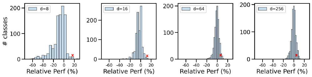
### Visual Description
\n
## Histograms: Relative Performance Distribution
### Overview
The image presents four histograms, each displaying the distribution of relative performance percentages. Each histogram corresponds to a different value of 'd' (8, 16, 64, and 256). Each histogram shows the number of classes (y-axis) against the relative performance percentage (x-axis). A red 'x' mark is present in each histogram, likely indicating a specific data point.
### Components/Axes
* **X-axis Label:** "Relative Perf (%)" - Represents the relative performance percentage, ranging from approximately -60% to +20%.
* **Y-axis Label:** "# classes" - Represents the number of classes, ranging from 0 to 200.
* **Histograms:** Four separate histograms, each with a light blue fill.
* **Legend:** Each histogram has a legend in the top-left corner indicating the value of 'd' for that histogram:
* d = 8
* d = 16
* d = 64
* d = 256
* **Red 'x' Markers:** A single red 'x' marker is present in each histogram.
### Detailed Analysis or Content Details
**Histogram 1 (d=8):**
* The distribution is centered around approximately -10% to 0%.
* The peak of the distribution is around -5%.
* The red 'x' is located at approximately 10% relative performance.
* The number of classes at the peak is approximately 190.
**Histogram 2 (d=16):**
* The distribution is centered around approximately -15% to 0%.
* The peak of the distribution is around -8%.
* The red 'x' is located at approximately 8% relative performance.
* The number of classes at the peak is approximately 180.
**Histogram 3 (d=64):**
* The distribution is centered around approximately -20% to 0%.
* The peak of the distribution is around -12%.
* The red 'x' is located at approximately 6% relative performance.
* The number of classes at the peak is approximately 170.
**Histogram 4 (d=256):**
* The distribution is centered around approximately -25% to 0%.
* The peak of the distribution is around -15%.
* The red 'x' is located at approximately 4% relative performance.
* The number of classes at the peak is approximately 160.
**Trend Verification:**
As 'd' increases, the distribution shifts to the left (more negative relative performance percentages) and the peak of the distribution decreases in height. The red 'x' also shifts to the right (more positive relative performance) with increasing 'd', but at a slower rate than the shift in the distribution.
### Key Observations
* The distributions are all approximately bell-shaped, suggesting a normal or near-normal distribution of relative performance.
* The center of the distribution shifts negatively as 'd' increases.
* The red 'x' consistently represents a relatively higher performance compared to the center of the distribution.
* The number of classes at the peak decreases as 'd' increases.
### Interpretation
The data suggests that as the value of 'd' increases, the typical relative performance decreases. The 'd' parameter likely represents a factor influencing performance, and higher values of 'd' lead to lower performance on average. The red 'x' could represent an outlier or a specific case with relatively high performance, even when 'd' is high. The shift in the distribution indicates a systematic effect of 'd' on performance, while the red 'x' suggests that individual cases can deviate from this trend. The decreasing peak height indicates a greater spread in performance as 'd' increases, meaning the outcomes are more variable. This could be due to increased sensitivity to other factors as 'd' increases.
</details>
Figure 12: Progression of relative per-class accuracy vs ${\rm MRL}$ -2048. As the dimensionality increases, the spread shrinks while the class marked (x) (Madagascar cat) loses accuracy.
In an attempt to derive an optimal routing policy to emulate oracle accuracy, we designed the adaptive classification via cascading method as discussed in Appendix D.1. This led to an interesting observation on the expected dimensionality for $76.30\%$ top-1 classification accuracy being just $d\sim 37$ . We leave the design and learning of a more optimal policy for future work.
Table 22: Percentage of ImageNet-1K validation set that is first correctly predicted using each representation size $d$ . We note that $18.46\%$ of the samples cannot be correctly predicted by any representation size. The remaining $81.54\%$ constitutes the oracle accuracy.
| Correctly Predicted | 67.46 | 8.78 | 2.58 | 1.35 | 0.64 | 0.31 | 0.20 | 0.12 | 0.06 | 18.46 |
| --- | --- | --- | --- | --- | --- | --- | --- | --- | --- | --- |
Table 23: Oracle classification accuracy of various evaluation datasets for ResNet50– ${\rm MRL}$ model trained on ImageNet-1K.
| FF–2048 ${\rm MRL}$ –Oracle | 76.9 81.5 | 64.9 70.6 | 3.6 8.7 | 35.1 39.8 | 23.7 28.9 |
| --- | --- | --- | --- | --- | --- |
Grad-CAM Examples
We analyzed the nature of model disagreement across representation sizes with ${\rm MRL}$ models with the help of Grad-CAM visualization [80]. We observed there were certain classes in ImageNet-1K such as "tools", "vegetables" and "meat cutting knife" which were occasionally located around multiple objects and a cluttered environment. In such scenarios, we observed that smaller representation size models would often get confused due to other objects and fail to extract the object of interest which generated the correct label. We also observed a different nature of disagreement arising when the models got confused within the same superclass. For example, ImageNet-1K has multiple "snake" classes, and models often confuse a snake image for an incorrect species of snake.
Superclass Performance
We created a 30 superclass subset of the validation set based on wordnet hierarchy (Table 24) to quantify the performance of ${\rm MRL}$ model on ImageNet-1K superclasses. Table 25 quantifies the performance with different representation size.
Table 24: 30 Superclasses in ImageNet-1K corresponding to the performance in Table 25.
| insect | motor vehicle | artiodactyl | vegetable | game equipment |
| --- | --- | --- | --- | --- |
| terrier | serpent | machine | measuring device | sheepdog |
| protective covering | sporting dog | vessel, watercraft | building | lizard |
| garment | hound | monkey | home appliance | wind instrument |
| vessel | fish | nourishment | electronic equipment | oscine |
| furniture | wading bird | tool | canine | mechanism |
Table 25: Performance of ${\rm MRL}$ model on 31-way classification (1 extra class is for reject token) on ImageNet-1K superclasses.
| ${\rm MRL}$ | 85.57 | 88.67 | 89.48 | 89.82 | 89.97 | 90.11 | 90.18 | 90.22 | 90.21 |
| --- | --- | --- | --- | --- | --- | --- | --- | --- | --- |
Appendix K Ablation Studies
K.1 ${\rm MRL}$ Training Paradigm
Table 26: Top-1 classification accuracy (%) on ImageNet-1K of various ResNet50 models which are finetuned on pretrained FF-2048 model. We observed that adding more non-linearities is able to induce nesting to a reasonable extent even if the model was not pretrained with nesting in mind.
| 8 16 32 | 5.15 13.79 32.52 | 36.11 58.42 67.81 | 54.78 67.26 71.62 | 60.02 70.10 72.84 | 66.63 73.53 75.03 |
| --- | --- | --- | --- | --- | --- |
| 64 | 52.66 | 72.42 | 73.61 | 74.29 | 75.82 |
| 128 | 64.60 | 74.41 | 74.67 | 75.03 | 76.30 |
| 256 | 69.29 | 75.30 | 75.23 | 75.38 | 76.47 |
| 512 | 70.51 | 75.96 | 75.47 | 75.64 | 76.65 |
| 1024 | 70.19 | 76.18 | 75.70 | 75.75 | 76.76 |
| 2048 | 69.72 | 76.44 | 75.96 | 75.97 | 76.80 |
${\rm Matryoshka~Representations}$ via Finetuning.
To observe if nesting can be induced in models that were not explicitly trained with nesting from scratch, we loaded a pretrained FF-2048 ResNet50 model and initialized a new ${\rm MRL}$ layer, as defined in Algorithm 2, Appendix C. We then unfroze different layers of the backbone to observe how much non-linearity in the form of unfrozen conv layers needed to be present to enforce nesting into a pretrained FF model. A description of these layers can be found in the ResNet50 architecture [29]. All models were finetuned with the FFCV pipeline, with same training configuration as in the end-to-end training aside from changing lr $=0.1$ and epochs $=10$ . We observed that finetuning the linear layer alone was insufficient to learn ${\rm Matryoshka~Representations}$ at lower dimensionalities. Adding more and more non-linear conv+ReLU layers steadily improved classification accuracy of $d=8$ from $5\%$ to $60\%$ after finetuning, which was only $6\%$ less than training ${\rm MRL}$ end-to-end for 40 epochs. This difference was successively less pronounced as we increased dimensionality past $d=64$ , to within $1.5\%$ for all larger dimensionalities. The full results of this ablation can be seen in Table 26.
Table 27: An ablation over boosting training loss at lower nesting dimensions, with top-1 and top-5 accuracy (%). The models are described in Appendix K.1.
| 8 16 32 | 66.63 73.53 75.03 | 84.66 89.52 91.31 | 69.53 73.86 75.28 | 86.19 89.44 91.21 | 69.24 73.91 75.10 | 85.96 89.55 91.14 |
| --- | --- | --- | --- | --- | --- | --- |
| 64 | 75.82 | 92.27 | 75.84 | 92.22 | 75.67 | 92.06 |
| 128 | 76.30 | 92.82 | 76.28 | 92.74 | 76.07 | 92.52 |
| 256 | 76.47 | 93.02 | 76.48 | 92.97 | 76.22 | 92.72 |
| 512 | 76.65 | 93.13 | 76.56 | 93.09 | 76.35 | 92.85 |
| 1024 | 76.76 | 93.22 | 76.71 | 93.21 | 76.39 | 92.98 |
| 2048 | 76.80 | 93.32 | 76.76 | 93.28 | 76.52 | 93.05 |
Relative Importance.
We performed an ablation of ${\rm MRL}$ over the relative importance, $c_{m}$ , of different nesting dimensions $m∈\cal{M}$ , as defined in Sec. 3. In an attempt to improve performance at lower dimensionalities, we boosted the relative importance $c_{m}$ of training loss at lower dimensions as in Eq. 1 with two models, ${\rm MRL}$ -8boost and ${\rm MRL}$ -8+16boost. The ${\rm MRL}$ -8boost model had $c_{m∈\cal M}=[2,1,1,1,1,1,1,1,1]$ and the ${\rm MRL}$ -8+16boost model had $c_{m∈\cal M}=[2,1.5,1,1,1,1,1,1,1]$ . The relative importance list $c_{m∈\cal M}$ had a 1-to-1 correspondence with nesting dimension set $\mathcal{M}$ . In Table 27, we observed that ${\rm MRL}$ -8boost improves top-1 accuracy by $3\%$ at $d=8$ , and also improves top-1 accuracy of all representation scales from 16 to 256 over ${\rm MRL}$ , while only hurting the performance at 512 to 2048 representation scales by a maximum of 0.1%. This suggests that the relative importance $c_{m}$ can be tuned/set for optimal accuracy for all $m∈\mathcal{M}$ , but we leave this extension for future work.
${\rm Matryoshka~Representations}$ at Arbitrary Granularities.
To train ${\rm MRL}$ , we used nested dimensions at logarithmic granularities $\mathcal{M}=\{8,16,...,1024,2048\}$ as detailed in Section 3. We made this choice for two empirically-driven reasons: a) The accuracy improvement with increasing representation size was more logarithmic than linear (as shown by FF models in Figure 3). This indicated that optimizing for granularities increasing in a non-logarithmic fashion would be sub-optimal both for maximum performance and expected efficiency; b) If we have $m$ arbitrary granularities, the expected cost of the linear classifier to train ${\rm MRL}$ scales as $O(L*(m^{2}))$ while logarithmic granularities result in $O(L*2log(d))$ space and compute costs.
To demonstrate this effect, we learned ${\rm Matryoshka~Representations}$ with uniform ( ${\rm MRL}$ -Uniform) nesting dimensions $m∈\mathcal{M}=\{8,212,416,620,824,1028,1232,1436,1640,1844,2048\}$ . We evaluated this model at the standard ( ${\rm MRL}$ -log) dimensions $m∈\mathcal{M}=\{8,16,32,64,128,256,512,1024,2048\}$ for ease of comparison to reported numbers using 1-NN accuracy (%). As shown in Table 29, we observed that while performance interpolated, ${\rm MRL}$ -Uniform suffered at low dimensions as the logarithmic spacing of ${\rm MRL}$ -log resulted in tighter packing of information in these initial dimensions. The higher nesting dimensions of ${\rm MRL}$ -Uniform did not help in significant accuracy improvement due to accuracy saturation, which is often logarithmic in representation size as shown by FF models. Note that the slight improvement at dimensions higher than 512 for ${\rm MRL}$ -Uniform is due to multiple granularities around them compared to just three for ${\rm MRL}$ -log, which are not useful in practice for efficiency.
Lower Dimensionality.
We experimented with training ${\rm MRL}$ with smaller nesting dimension than $m=8$ , as shown in Table 29, with two models: MRL-4 and MRL-6. We found that using lower than 8-dimensions to train ${\rm MRL}$ , i.e. $m_{0}∈\{4,6\}$ for MRL-4 and MRL-6 respectively, did not affect the top-1 accuracy of other granularities significantly. However, granularities smaller than 8-dimensions had very low accuracy and were often unusable for deployment along with additional training difficulty. We also observed a small dip in accuracy at higher dimensions which we attribute to the joint loss that now also included the harder optimization of the smallest dimension. Lastly, we hypothesize the dimensionality of 8 is an empirically validated design choice due to the considerable accuracy it provided along with the ease of training.
Table 28: An ablation over training with smaller nesting dimensionalities in terms of Top-1 accuracy (%). MRL-4 and MRL-6 are variations of the original model (MRL-8) with $m_{0}∈\{4,6\}$ , where $m∈\mathcal{M}$ is part of the nesting_list as seen in Alg 2.
| 4 6 8 | 27.25 - 66.86 | - 58.71 67.55 | - - 66.63 |
| --- | --- | --- | --- |
| 16 | 73.36 | 73.10 | 73.53 |
| 32 | 74.82 | 74.49 | 75.03 |
| 64 | 75.51 | 75.32 | 75.82 |
| 128 | 75.93 | 75.61 | 76.30 |
| 256 | 76.08 | 75.82 | 76.47 |
| 512 | 76.31 | 75.93 | 76.65 |
| 1024 | 76.38 | 76.04 | 76.76 |
| 2048 | 76.43 | 76.12 | 76.80 |
Table 29: An ablation over training ${\rm MRL}$ with nesting list at uniformly distributed granularities. Entries in the ${\rm MRL}$ -Uniform column are evaluated at logarithmic dimensions for a fair comparison to ${\rm MRL}$ -Log (standard ${\rm MRL}$ ) with 1-NN accuracy (%).
| 8 16 32 | 62.19 67.91 69.46 | 58.44 61.11 63.82 |
| --- | --- | --- |
| 64 | 70.17 | 66.44 |
| 128 | 70.52 | 68.71 |
| 256 | 70.62 | 70.06 |
| 512 | 70.82 | 70.98 |
| 1024 | 70.89 | 71.37 |
| 2048 | 70.97 | 71.44 |
K.2 Retrieval
Adaptive Retrieval.
To examine the effect of increasing shortlist lengths on search time, we performed a reranking ablation over shortlist lengths for $D_{s}$ = 16 and $D_{r}$ = 2048 over ImageNet-1K in Table 30, and over ImageNet-4K in Table 31. We observed that using a larger shortlist $k$ saturated ImageNet-1K performance at $k$ =200. But using larger shortlists until $k=2048$ , the maximum value supported by the FAISS framework, steadily improved performance on ImageNet-4K. This is likely due to the increased database size, but could also indicate a correlation with ImageNet-4K being slightly out-of-distribution making the task at hand harder.
Table 30: Adaptive retrieval ablation over shortlist length $k$ for $D_{s}=16$ , $D_{r}=2048$ on ImageNet-1K with exact search. Entries with the highest P@1 and mAP@10 across all $k$ are in bold.
| 100 200 400 | 70.88 70.90 70.94 | 65.19 65.27 65.26 | 63.62 63.73 63.71 | 62.59 62.82 62.81 | 61.24 61.97 62.03 | 69.96 70.10 70.15 | 69.24 69.44 69.51 | 68.53 68.90 69.02 | 67.20 68.21 68.47 |
| --- | --- | --- | --- | --- | --- | --- | --- | --- | --- |
| 800 | 70.96 | 65.23 | 63.64 | 62.69 | 61.85 | 70.16 | 69.52 | 69.02 | 68.45 |
| 1600 | 70.96 | 65.20 | 63.58 | 62.58 | 61.66 | 70.16 | 69.5 | 68.97 | 68.36 |
| 2048 | 70.97 | 65.20 | 63.57 | 62.58 | 61.64 | 70.16 | 69.5 | 68.97 | 68.35 |
Table 31: Adaptive retrieval ablation over shortlist length $k$ for $D_{s}=16$ , $D_{r}=2048$ on ImageNet-4K with exact search.
| 100 200 400 | 27.70 28.56 29.34 | 14.38 15.21 15.83 | 10.62 11.43 12.06 | 8.26 9.11 9.76 | 6.07 7.12 7.79 | 20.12 21.23 22.08 | 16.87 18.13 19.09 | 14.29 15.73 16.83 | 11.26 13.27 14.54 |
| --- | --- | --- | --- | --- | --- | --- | --- | --- | --- |
| 800 | 29.86 | 16.30 | 12.53 | 10.23 | 8.26 | 22.72 | 19.83 | 17.65 | 15.45 |
| 1600 | 30.24 | 16.63 | 12.86 | 10.56 | 8.60 | 23.18 | 20.36 | 18.23 | 16.11 |
| 2048 | 30.35 | 16.73 | 12.96 | 10.65 | 8.69 | 23.31 | 20.50 | 18.40 | 16.30 |