2206.09557

# ArXiv Paper 2206.09557v1 ## nuQmm: Quantized MatMul for Efficient Inference of Large-Scale Generative Language Models Gunho Park ∗† , Baeseong Park ∗‡ , Se Jung Kwon ‡ , Byeongwook Kim ‡ , Youngjoo Lee † , and Dongsoo Lee ‡ † Pohang University of Science and Technology, Pohang, Republic of Korea { gunho1123, youngjoo.lee } @postech.ac.kr ‡ NAVER CLOVA, Seongnam, Republic of Korea { baeseong.park, sejung.kwon, byeonguk.kim, dongsoo.lee } @navercorp.com Abstract -The recent advance of self-supervised learning associated with the Transformer architecture enables natural language processing (NLP) to exhibit extremely low perplexity. Such powerful models demand ever-increasing model size, and thus, large amounts of computations and memory footprints. In this paper, we propose an efficient inference framework for largescale generative language models. As the key to reducing model size, we quantize weights by a non-uniform quantization method. Then, quantized matrix multiplications are accelerated by our proposed kernel, called nuQmm, which allows a wide trade-off between compression ratio and accuracy. Our proposed nuQmm reduces the latency of not only each GPU but also the entire inference of large LMs because a high compression ratio (by low-bit quantization) mitigates the minimum required number of GPUs. We demonstrate that nuQmm can accelerate the inference speed of the GPT-3 (175B) model by about 14.4 times and save energy consumption by 93%. Index Terms -Non-Uniform Quantization, Model Compression, Generative Language Model, Deep Learning, Transformer, AI Inference ## I. INTRODUCTION Recent years have observed large-scale language models presenting state-of-the-art performance on various natural language process (NLP) tasks. Such rapid progress in NLP performance has been highly facilitated by the self-supervised learning method. Through self-supervised learning, a model is first pre-trained by using unlabeled data and then finetuned by a small number of labeled data [1]-[4]. Since pre-training dominates the entire training process without an expensive labeling process, the size of the training dataset can substantially increase. Combined with efficient sequence-tosequence model architectures, such as the Transformers [5], the number of model parameters also significantly increases. 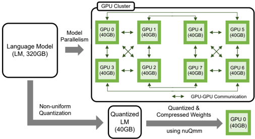As for NLP tasks, it is reported that LM performance follows predictable power-law scaling as a function of model size [6], [7]. Since then, especially for generative LMs, researchers proposed numerous large-scale models including GPT-3 (175B) [6], HyperCLOVA (204B) [8], Gopher (280B) [9], and Megatron Turing NLG (530B) [10]. Note that models of billions of parameters cannot be accommodated by one GPU since GPU memory size is sacrificed and limited in order to enhance memory bandwidth [11], [12]. To address such concerns, model parallelism has been suggested to distribute computations over multiple GPUs through GPU-to-GPU communication [13], [14]. As shown in Fig. 1, model parallelism Fig. 1. A large language model deployed with 8 GPUs supported by model parallelism, or with 1 GPU only using quantized weights. Assuming 40GB GPU memory size, 8 GPUs are required to serve a 320GB language model unless model compression is engaged. <details> <summary>Image 1 Details</summary>  ### Visual Description ## Diagram: Language Model Processing Workflow with GPU Cluster ### Overview The diagram illustrates a technical workflow for processing a large language model (LM) across a GPU cluster, emphasizing model parallelism, quantization, and compression techniques. The LM (320GB) is distributed across 8 GPUs (each 40GB) via model parallelism, with additional paths for non-uniform quantization and weight compression using nuQmm. ### Components/Axes - **Language Model (LM)**: 320GB, input to the workflow. - **Model Parallelism**: Splits the LM across 8 GPUs (GPU 0–7), each with 40GB capacity. - **GPU Cluster**: Contains 8 GPUs (GPU 0–7), interconnected with bidirectional communication arrows. - **Non-uniform Quantization**: Reduces LM size to 40GB. - **Quantized & Compressed Weights**: Further optimized using nuQmm, stored in GPU 0 (40GB). - **Arrows**: Indicate data flow (e.g., GPU-GPU communication, quantization paths). ### Detailed Analysis 1. **Model Parallelism**: - The 320GB LM is split across 8 GPUs (GPU 0–7), each handling 40GB. Arrows show bidirectional communication between GPUs (e.g., GPU 0 ↔ GPU 1, GPU 3 ↔ GPU 2). - GPUs are arranged in two rows (top: GPU 0–5; bottom: GPU 3–7), with diagonal arrows suggesting inter-GPU data exchange. 2. **Quantization Path**: - Non-uniform quantization reduces the LM from 320GB to 40GB, bypassing the GPU cluster. 3. **Compression Path**: - Quantized weights are further compressed using nuQmm, resulting in a 40GB model stored in GPU 0. ### Key Observations - **Memory Optimization**: The workflow demonstrates how quantization and compression reduce the LM’s memory footprint from 320GB to 40GB, enabling deployment on a single GPU (GPU 0). - **Parallelism Overhead**: Despite parallelism, GPU-GPU communication is required, implying potential latency or bandwidth constraints. - **Final Output**: The compressed model resides solely in GPU 0, suggesting a centralized deployment after distributed processing. ### Interpretation This diagram highlights strategies for deploying large language models on constrained hardware. Model parallelism distributes the workload across GPUs, while quantization and compression optimize memory usage. The bidirectional GPU communication indicates collaborative processing, but the final compressed model’s isolation in GPU 0 suggests a trade-off between distributed training and centralized inference. The use of nuQmm for compression implies a focus on efficiency without sacrificing model performance. The workflow underscores the balance between scalability (parallelism) and resource constraints (quantization/compression). </details> splits parameters of a large LM model into numerous GPUs, and information during training/inference can be shared among GPUs through dedicated channels. Model parallelism can be divided into tensor parallelism and pipeline parallelism to improve latency and throughput, respectively. Such parallelism schemes, however, require various communication primitives, such as AllReduce , Reduce , Broadcast , and AllGather , to synchronize partial outputs produced by GPUs [15]. Even though GPU-specific external communication protocols (e.g., NVLink [16]) can reduce communication latency, an inherent variance of GPU performance (caused by various random factors such as fabrication process variation and operating system conditions) is another performance bottleneck [17]. In addition, since a large matrix is separated into submatrices, each GPU faces tall-andskinny matrix multiplications with low utilization of resources [18], [19]. As a result, performance gain by model parallelism becomes a sub-linear function of the number of GPUs. To alleviate the challenges of model parallelism, parameter quantization [20]-[22] is a practical solution to reduce the model size such that the number of GPUs to serve inference can be lower, as described in Fig. 1. Among various quantization schemes, uniform quantization is a popular choice since we can exploit integer-based arithmetic units [23]-[26]. 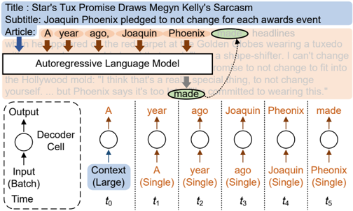Uniform quantization, however, is practically limited to 8 bits Fig. 2. An illustration of the autoregressive language model. Given an input context, a single token is generated for each iteration. The entire generation procedure can be categorized into the summarization stage (along with a large batch size using an input context) and the generation stage executing singlebatch operations using the previously generated token. <details> <summary>Image 2 Details</summary>  ### Visual Description ## Diagram: Autoregressive Language Model Processing Flow ### Overview The diagram illustrates the architecture and processing flow of an autoregressive language model. It shows how input text is processed sequentially through decoder cells over time to generate output text. The example uses a news article about Joaquin Phoenix's commitment to wearing a tuxedo as input context. ### Components/Axes 1. **Input (Batch)**: - Represents the initial text context provided to the model. - Example: "A year ago, Joaquin Phoenix made headlines..." 2. **Decoder Cell**: - Processes sequential input tokens over time to generate output. - Outputs predictions for the next token in the sequence. 3. **Time Steps (t₀ to t₅)**: - Sequential processing of individual tokens. - Labels: - t₀: "A" - t₁: "year" - t₂: "ago" - t₃: "Joaquin" - t₄: "Phoenix" - t₅: "made" 4. **Output**: - Final prediction from the decoder cell at each time step. ### Detailed Analysis - **Input Context**: The model starts with a large context window containing the full article text. - **Tokenization**: The input is broken into individual tokens (words) processed sequentially. - **Sequential Processing**: - At t₀, the model processes "A" and begins building context. - By t₅, the model predicts "made" based on prior tokens ("A year ago, Joaquin Phoenix"). - **Flow**: Arrows indicate the direction of information flow from input tokens to the decoder cell and then to the output. ### Key Observations 1. **Contextual Dependency**: Each token's prediction depends on all prior tokens in the sequence. 2. **Temporal Progression**: The model processes tokens in strict chronological order (t₀ → t₅). 3. **Output Generation**: The final output ("made") is generated after incorporating all preceding tokens. ### Interpretation This diagram demonstrates the core mechanism of autoregressive models: - **Sequential Prediction**: The model generates text one token at a time, using prior tokens as context. - **Example Application**: The input text about Joaquin Phoenix's tuxedo commitment is used to show how the model would predict the next word ("made") in the sentence. - **Technical Insight**: The decoder cell's role in maintaining and updating context over time is critical for coherent text generation. **Note**: No numerical data or quantitative trends are present in this conceptual diagram. The focus is on architectural components and processing flow. </details> while non-linear operations (e.g., softmax and normalization techniques) can be imprecise [27], [28]. Moreover, activation quantization/dequantization should be implemented on-thefly on top of the requirement of accurate estimation of the distribution of activations in advance. In this paper, we consider non-uniform quantization to achieve a high compression ratio. Specifically, we utilize binary-coding quantization (BCQ) scheme [29] to gain benefits of simple arithmetic operations. Note that non-uniform quantization inherently relies on customized hardware to support bit-level operations. To enable efficient BCQ scheme for inference on GPUs, we propose a new BCQ-dedicated matrix multiplication kernel, called nuQmm, to obtain low inference latency while avoiding the necessity of activation quantization. Our major contributions in this work include the following: - Compared to the previously proposed matrix multiplication kernels with quantized parameters, nuQmm provides a wide search space of trade-offs between compression ratio and latency (based on GPU-specific efficient hardware utilization method to implement various BCQ formats). - Under such new search space, we quantize a few wellknown generative LMs, such as GPT-2 and GPT Neo, to investigate the range of compression ratio achievable by nuQmm. - For large LMs, we show that nuQmm can considerably accelerate matrix multiplications with small quantization bits while power consumption is saved a lot by reducing the number of GPUs. Consequently, nuQmm leads to low energy consumption. - In the case of GPT-3 (175B), our experimental results show that matrix multiplications can be accelerated by about 14.4 times while overall energy consumption can be saved by 93%. TABLE I SIZES, ARCHITECTURES, AND RELEASE TYPES OF VARIOUS GENERATIVE LANGUAGE MODELS | Model Name | n params | n layers | d model | Release | |--------------|------------|------------|-----------|-----------| | GPT-2 Small | 124M | 12 | 768 | Public | | GPT-2 Medium | 355M | 24 | 1024 | Public | | GPT-2 Large | 774M | 36 | 1280 | Public | | GPT-2 XL | 1.5B | 48 | 1600 | Public | | GPT Neo 1.3B | 1.3B | 24 | 2048 | Public | | GPT Neo 2.7B | 2.7B | 32 | 2560 | Public | | GPT-J 6B | 6.1B | 28 | 4096 | Public | | GPT-3 6.7B | 6.7B | 32 | 4096 | Private | | GPT-3 13B | 13.0B | 40 | 5140 | Private | | GPT-3 175B | 175.0B | 96 | 12288 | Private | | MT-NLG | 530.0B | 105 | 20480 | Private | ## II. BACKGROUND ## A. Generative Language Models Well-known large-scale generative LMs, such as GPT-3, are autoregressive models that predict future tokens using the previous tokens in a feed-forward fashion. For example, as shown in Fig. 2, assuming an input context is given (for in-context learning [6]), a new token can be predicted by using the previously generated tokens. Correspondingly, autoregressive modeling employs both large-batch operations (for the summarization stage conducting in-context learning using a given input context) and single-batch operations (for the generation stage to generate a single token at a time index). Since the Transformer introduced a self-attention mechanism and a parallelized training algorithm for autoregressive models using a teacher forcing technique [5], virtually all large-scale generative LMs follow the decoder structure of the Transformer. In addition to the architectural advantages of the Transformer to scale the model size, generative LMs are increasing the number of parameters (as depicted in Table I) because: 1) self-supervised learning alleviates the burden of the expensive labeling process and 2) scaling-law [6], [7] provides a predictable performance on the cross-entropy loss as the model size increases. Surprising qualitative evaluation results (e.g., human-like writing) of extreme-scale LMs also fueled the competition in model size [8], [9]. ## B. 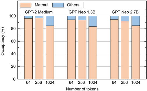GPU-Accelerated Generative LMs For the Transformers and their variants, the processing time of matrix multiplications dominates the entire inference latency because of higher time complexity compared to activation functions, normalization layers, and so on [27], [28], [30]. To validate such a claim, Fig. 3 shows the latency breakdown of representative large-scale generative LMs (GPT-2 Medium, GPT Neo 1.3B, and GPT Neo 2.7B) with a various number of tokens to be generated. Fig. 3 is obtained by RTX-3090 and FasterTransformer inference framework of Nvidia 1 . We can observe that matrix multiplications dominate the entire processing time (at least 80%) for various LM sizes and tokens to be generated. Hence, GPUs are widely adopted to accelerate inference because GPUs embed lots of arithmetic units and 1 https://github.com/NVIDIA/FasterTransformer Fig. 3. Latency breakdown of GPT models with a different number of tokens to be generated. The overall performance is dominated by MatMul operations especially when a larger model size and a small number of tokens are employed. Experiments are conducted with RTX-3090 and FasterTransformer inference framework. <details> <summary>Image 3 Details</summary>  ### Visual Description ## Bar Chart: Model-Specific Occupancy by Token Count ### Overview The chart compares occupancy percentages (Matmul vs. Others) across three AI models (GPT-2 Medium, GPT Neo 1.3B, GPT Neo 2.7B) at three token counts (64, 256, 1024). Occupancy is visualized as stacked bars, with Matmul (orange) and Others (blue) segments. ### Components/Axes - **X-axis**: "Number of tokens" (64, 256, 1024) - **Y-axis**: "Occupancy (%)" (0–100) - **Legend**: - Orange = Matmul - Blue = Others - **Model Groups**: - GPT-2 Medium (leftmost group) - GPT Neo 1.3B (middle group) - GPT Neo 2.7B (rightmost group) ### Detailed Analysis - **GPT-2 Medium**: - 64 tokens: Matmul ~95%, Others ~5% - 256 tokens: Matmul ~95%, Others ~5% - 1024 tokens: Matmul ~85%, Others ~15% - **GPT Neo 1.3B**: - 64 tokens: Matmul ~90%, Others ~10% - 256 tokens: Matmul ~90%, Others ~10% - 1024 tokens: Matmul ~80%, Others ~20% - **GPT Neo 2.7B**: - 64 tokens: Matmul ~90%, Others ~10% - 256 tokens: Matmul ~85%, Others ~15% - 1024 tokens: Matmul ~80%, Others ~20% ### Key Observations 1. **Matmul Dominance**: Matmul consistently occupies >80% of total occupancy across all models and token counts. 2. **Token Count Impact**: - Matmul occupancy decreases slightly as token count increases (e.g., 95% → 85% for GPT-2 Medium at 1024 tokens). - Others occupancy increases with token count (e.g., 5% → 15% for GPT-2 Medium at 1024 tokens). 3. **Model-Specific Trends**: - GPT-2 Medium maintains the highest Matmul occupancy. - GPT Neo 2.7B shows the largest drop in Matmul occupancy (90% → 80%) at 1024 tokens. ### Interpretation The data suggests that Matmul operations dominate computational resources for smaller token counts, but their efficiency diminishes as token size grows. The increasing share of "Others" (likely non-Matmul operations) at higher token counts implies that larger workloads require more diverse computational resources. GPT-2 Medium appears more Matmul-efficient than the GPT Neo variants, potentially indicating architectural differences in how these models handle matrix operations. The trend of declining Matmul efficiency with scale aligns with expectations for memory-bound workloads, where larger token sizes may introduce overhead from data movement or non-linear operations. </details> support multiple threads that are critical to expediting matrix multiplications [11], [14]. Note that extracting high performance from GPUs depends on arithmetic intensity. In other words, batch size should be large enough to ensure a high reuse ratio of data once retrieved from main memory [31]. In the extreme case of a single batch, matrix multiplication becomes memory-bound (in the form of a matrix-vector multiplication) such that utilization of internal arithmetic units is forced to be low. As such, for the generation stage (shown in Fig. 2) requiring single-batch operations, we can expect the speed of GPUs running generative LM inference to be far from peak performance. Another issue with running GPUs for inference is that GPUs have prioritized high memory bandwidth over memory size [31], [32]. Consequently, large LMs need to be distributed across multiple GPUs so as to incur GPU-to-GPU communication overhead. ## C. Binary-Coding Quantization Quantization reduces the number of bits to represent model parameters. Shrinking memory footprint by quantization for generative LMs is effective to address the concerns on GPU performance, namely, 1) memory-bound single-batch operations for generating tokens and 2) the usage of multiple GPUs and associated communication overhead. Note that various uniform quantization methods are being intensively studied because uniform quantization can be implemented by simple fixed-point operations [24], [27], [28], [33]. On the other hand, non-uniform quantization usually demands complicated operations of low parallelism while supporting hardware instructions may not be available [20], [34]. In this paper, we choose binary-coding quantization (BCQ), first introduced in [29], which is one of the non-uniform quantization schemes. When a weight vector w (of size n ) is quantized by BCQ and q is the number of quantization bits, w is approximated to be ∑ q i =1 α i b i where α i ∈ R + is a scaling factor and b i ∈ {-1 , +1 } n is a binary vector. Note that a scaling factor α can be shared by many weights ( n can be any number) such that larger n value results in a relatively smaller memory footprint for scaling factors. The quantization process broadly involves finding scaling factors and binary vectors to minimize the quantization error as follows: $$\arg \min _ { a , b } | w - \sum _ { i = 1 } ^ { q } a _ { i } b _ { i } | ,$$ ∥ ∥ which does not have analytical solutions except when q = 1 . Thus, scaling factors and binary vectors are obtained by iterative search methods [20], [34] or by quantization-aware training [30]. In this work, we discuss the unique mathematical properties of BCQ to enable efficient quantized matrix multiplications. ## III. DESIGN METHODOLOGY OF NUQMM Our overall goal is to explore high-performance and lowenergy inference systems for large-scale generative language models such as GPT-3 175B. To this end, an efficient quantization method is supposed to compress models with a high compression ratio while reducing quantization error (for given quantization bits) in consideration of the characteristics of large-scale LMs. In addition, a new kernel that efficiently supports such an efficient quantization technique is also necessary so that latency improvement through quantization can be maximized. In this section, we propose new advanced BCQ formats that can be supported by our proposed kernel nuQmm. The proposed nuQmm is designed to directly utilize binary weights in a compressed format without additional overhead such as dequantization. As a result, we demonstrate that we can reduce the number of GPUs to run large-scale LM inference. ## A. Group-wise Binary-Coding Quantization In practice, conventional BCQ methods assume that a scaling factor is assigned to each row of a weight matrix (or even to the entire matrix) so as to support vector instructions of CPUs or GPUs [20], [29]. As large-scale LMs introduce deeper and wider model structures along with ever-increasing parameter size [9], [13], however, we argue that such conventional row-wise BCQ format encounters various challenges. Suppose that a relatively small hidden size (e.g., d model = 1024 in Table I) is selected along with small weight matrices correspondingly, row-wise assignment of scaling factors might be reasonable to obtain low quantization error. On the other hand, if the hidden size increases rapidly (e.g., d model = 12288 for GPT-3 175B in Table I) according to the advent of largescale LMs, it would be more difficult to compute a proper scaling factor shared by a larger number of weights. One possible solution to lower quantization error is to increase the number of quantization bits. Such a method, however, sacrifices the compression ratio considerably in a regime of low-bit quantization. As a result, for a given number of quantization bits, it is necessary to investigate different ways of assigning scaling factors as long as a new assignment can be backed by practical implementation. 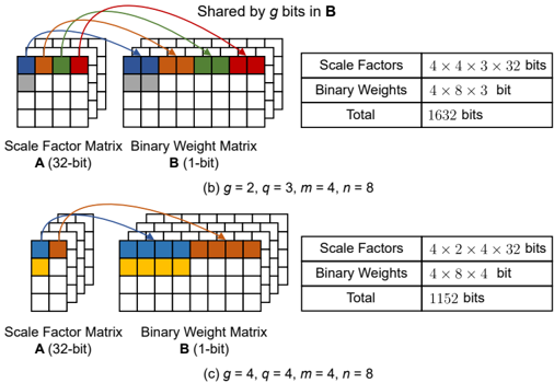| Scale Factors | bits | |-----------------|--------------------------------| | Binary Weights | bit | | Total Space | Scale Factors + Binary Weights | (a) Space complexity | Scale Factors | bits | |-----------------|--------| | Binary Weights | bit | | Total | bits | | Scale Factors | bits | |-----------------|--------| | Binary Weights | bit | | Total | bits | Fig. 4. Group-wise BCQ example with two different ( g, q ) configurations to quantize an ( 8 × 8 ) matrix. Assuming a scaling factor of 32 bits, smaller q can yield a larger memory footprint if g is also small. <details> <summary>Image 4 Details</summary>  ### Visual Description ## Diagram: Scale Factor and Binary Weight Matrix Configuration ### Overview The image presents two technical diagrams (labeled **b** and **c**) illustrating the configuration of **Scale Factor Matrix A** (32-bit) and **Binary Weight Matrix B** (1-bit), with shared bits in B. Each diagram includes a table summarizing the bit allocation for scale factors, binary weights, and total bits. The diagrams use color-coded arrows to indicate shared bits and spatial relationships between matrices. --- ### Components/Axes 1. **Matrices**: - **Scale Factor Matrix A**: 32-bit values, represented as a grid with colored blocks (blue, orange, green, red). - **Binary Weight Matrix B**: 1-bit values, represented as a grid with uniform blocks. - Arrows connect Scale Factor Matrix A to Binary Weight Matrix B, labeled "Shared by *g* bits in B." 2. **Tables**: - **Scale Factors**: Dimensions and total bits (e.g., `4 × 4 × 3 × 32 bits`). - **Binary Weights**: Dimensions and total bits (e.g., `4 × 8 × 3 bits`). - **Total**: Sum of scale factors and binary weights (e.g., `1632 bits`). 3. **Parameters**: - **g**: Number of shared bits in B (e.g., `g = 2` in diagram **b**, `g = 4` in diagram **c**). - **q, m, n**: Dimensions influencing matrix sizes (e.g., `q = 3`, `m = 4`, `n = 8` in diagram **b**). --- ### Detailed Analysis #### Diagram **b** (`g = 2`, `q = 3`, `m = 4`, `n = 8`): - **Scale Factors**: `4 × 4 × 3 × 32 bits` - Total: `4 × 4 × 3 × 32 = 1,536 bits`. - **Binary Weights**: `4 × 8 × 3 bits` - Total: `4 × 8 × 3 = 96 bits`. - **Total**: `1,536 + 96 = 1,632 bits`. #### Diagram **c** (`g = 4`, `q = 4`, `m = 4`, `n = 8`): - **Scale Factors**: `4 × 2 × 4 × 32 bits` - Total: `4 × 2 × 4 × 32 = 1,024 bits`. - **Binary Weights**: `4 × 8 × 4 bits` - Total: `4 × 8 × 4 = 128 bits`. - **Total**: `1,024 + 128 = 1,152 bits`. **Key Observations**: 1. **Shared Bits (`g`)**: - In **b**, `g = 2` bits are shared between A and B. - In **c**, `g = 4` bits are shared, reducing redundancy. 2. **Matrix Dimensions**: - Scale Factor Matrix A’s first dimension scales as `n/g` (e.g., `8/2 = 4` in **b**, `8/4 = 2` in **c**). - Binary Weight Matrix B’s third dimension scales with `q` (e.g., `q = 3` in **b**, `q = 4` in **c**). 3. **Total Bit Reduction**: Increasing `g` from 2 to 4 reduces total bits from 1,632 to 1,152, demonstrating efficiency gains from shared bits. --- ### Interpretation 1. **Efficiency Trade-offs**: - Higher `g` values (shared bits) reduce the Scale Factor Matrix size (`n/g`) but increase Binary Weight Matrix size (`q`). However, the net effect is lower total bits, suggesting optimized memory usage. - Example: In **c**, doubling `g` (from 2 to 4) halves the Scale Factor dimension (`4 → 2`) while increasing Binary Weights (`3 → 4`), but total bits drop by 30%. 2. **Hardware Implications**: - This configuration likely targets applications like neural networks, where 32-bit precision (Scale Factors) and 1-bit weights (Binary Weights) balance accuracy and efficiency. - Shared bits (`g`) may represent quantized or compressed data paths, critical for low-power hardware. 3. **Anomalies**: - No outliers; trends align with parameter definitions. The reduction in total bits with higher `g` is consistent across diagrams. --- ### Key Takeaways - **Shared Bits (`g`)**: Directly impact memory efficiency by reducing Scale Factor dimensions while increasing Binary Weight granularity. - **Parameter Interplay**: `n`, `q`, and `m` define matrix sizes, with `g` acting as a compression factor. - **Practical Use**: Enables efficient storage and computation in hardware-accelerated AI models, balancing precision and resource constraints. </details> - a) Group-wise α Assignment: As an alternative to rowwise quantization, we propose group-wise quantization in which a scaling factor can be shared by an arbitrary number of weights. Our proposed new BCQ format introduces a new hyper-parameter g as a group size that represents the number weights to be shared by a scaling factor. In this paper, g is a fixed number with a range of 8 (as the minimum) to the column width of a matrix (equivalent to row-wise quantization). Since g is a constant number, the hidden size does not affect our group-wise BCQ formats. We discuss how to implement the proposed group-wise BCQ efficiently on GPUs later. b) Impact on Compression Ratio: For a given q (i.e., the number of quantization bits), a smaller group size g can lower quantization error at the expense of increased memory footprint for scaling factors. For a target quantization error, thus, a compression ratio is a compromise between q and g . In other words, due to the introduction of g , we can control the amount of scaling factors and binary vectors as a trade-off process. Note that the memory footprint of conventional rowwise quantization techniques is dominated by the size of binary vectors because the size of scaling factors is usually ignorable if the column width of a matrix is large enough. Compared to the conventional scheme, our proposed group-wise BCQ provides a new wide search space for quantization formats to meet a target compression ratio. Fig. 4 shows an example with two ( g, q ) configurations to quantize an ( 8 × 8 ) matrix. Indeed, even if the number of quantization bits is smaller, the memory footprint can be large when the group size g is small (i.e., more scaling factors are employed). 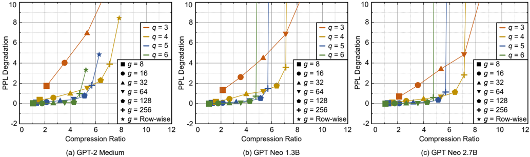c) Exploration of Compression Ratio: To study the capability of group-wise BCQ to enlarge search space for com- pression, we conduct experiments using GPT-2 Medium 2 , GPT Neo 3 1.3B and 2.7B whose pre-trained models are publicly available. Specifically, we apply post-training quantization (with an iterative solver introduced in [20]) to those three pre-trained models while g and q vary. Then, each quantized model is evaluated on the WikiText-2 dataset to obtain the perplexity (PPL) to find the relationship between compression ratio and PPL. Fig. 5 shows PPL degradation and compression ratio 4 when we try various q values (from 3 to 6) and g values (from 8 to matrix column width (i.e., row-wise)). From Fig. 5, we observe that the relationship between PPL degradation and g are vastly different depending on q . As a result, compared to the conventional row-wise quantization, group-wise BCQ offers new optimal configurations. For example in the case of the GPT-2 Medium model in Fig. 5, when a target PPL degradation is around 4.0, then 4-bit quantization is superior to 3-bit quantization in terms of compression ratio (even though g values are different). Thus, for a target PPL degradation (or a target compression ratio), we need to explore various q and g values simultaneously to achieve the best compression ratio (or the minimum PPL degradation). Note that for GPT Neo 1.3B and 2.7B, as we discussed the limits of row-wise quantization for large-scale LMs, a small g value is critical to achieving low PPL degradation. All in all, the effects of q and g on accuracy differ with each model such that q and g are hyper-parameters to be optimized. 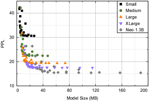Fig. 6 describes PPL (of four GPT-2 models with different sizes and one GPT Neo model) when diversified model sizes for each model are available by exploring q and g values. Even though we adopt post-training quantization instead of quantization-aware training (that might be too expensive for recent large LMs), the sizes of all 5 models in Fig. 6 are reduced a lot by our group-wise quantization. Suppose that we can tolerate some reasonable PPL degradation, we notice that larger models tend to be compressed by a higher compression ratio, which is consistent with a report in [35]. In the next subsections, we study a matrix multiplication kernel to facilitate the potential benefits of group-wise BCQ formats. ## B. Quantized Matrix Multiplication based on Lookup Tables Under our quantization scheme that quantizes weights by using BCQ format and maintains activations to be fullprecision, naive matrix multiplications result in duplicate and redundant partial computations. To illustrate, assume that a binary matrix B ∈ {-1 , +1 } 4 × 4 and an activation vector x ∈ R 4 are given as $$B = \begin{bmatrix} + 1 - 1 - 1 + 1 \\ + 1 - 1 - 1 + 1 \\ - 1 + 1 - 1 + 1 \\ - 1 + 1 - 1 + 1 \end{bmatrix} , x ^ { T } = \begin{bmatrix} - 0.7 0.3 0.6 \\ - 0.7 0.3 0.6 \end{bmatrix} . (2)$$ Then, computing Bx /latticetop (that is to be multiplied by scaling factors) would repeat (1 . 2 -( -0 . 7)) three times and ( -0 . 3 + 2 https://huggingface.co/gpt2-medium 3 https://huggingface.co/EleutherAI 4 Calculated as FP32 model size divided by each quantized model size. Fig. 5. PPL degradation and compression ratio with the various number of quantization bits ( q ) and group size ( g ). Three pre-trained models are quantized (by post-training quantization method) and then evaluated on the WikiText-2 dataset. <details> <summary>Image 5 Details</summary>  ### Visual Description ## Line Chart: PPL Degradation vs Compression Ratio for GPT Models ### Overview Three line charts compare perplexity (PPL) degradation against compression ratio for three GPT variants: GPT-2 Medium, GPT Neo 1.3B, and GPT Neo 2.7B. Each chart shows multiple data series representing different quantization (q) and grouping (g) parameters, with distinct markers and colors for each series. ### Components/Axes - **X-axis**: Compression Ratio (0–12, linear scale) - **Y-axis**: PPL Degradation (-2–10, linear scale) - **Legends**: - **q values**: Quantization levels (3, 4, 5, 6) with distinct colors: - q=3: Red (square) - q=4: Orange (circle) - q=5: Blue (triangle) - q=6: Green (star) - **g values**: Grouping parameters (8, 16, 32, 64, 128, 256, Row-wise) with distinct markers: - g=8: Square - g=16: Circle - g=32: Triangle - g=64: Diamond - g=128: Pentagon - g=256: Hexagon - Row-wise: Star ### Detailed Analysis #### Chart (a) GPT-2 Medium - **q=3 (Red)**: Steep upward slope, reaching ~8 PPL at compression ratio 10. - **q=4 (Orange)**: Gradual increase, peaking at ~6 PPL at ratio 10. - **q=5 (Blue)**: Moderate rise, ~4 PPL at ratio 10. - **q=6 (Green)**: Slowest increase, ~2 PPL at ratio 10. - **g values**: All g series (8–256) cluster near 0–2 PPL until ratio ~6, then diverge sharply. Row-wise (star) shows a unique spike at ratio 8 (~8 PPL). #### Chart (b) GPT Neo 1.3B - **q=3 (Red)**: Sharp rise, ~7 PPL at ratio 10. - **q=4 (Orange)**: Steady increase, ~5 PPL at ratio 10. - **q=5 (Blue)**: Moderate growth, ~3 PPL at ratio 10. - **q=6 (Green)**: Minimal degradation, ~1 PPL at ratio 10. - **g values**: Similar clustering as GPT-2, but Row-wise (star) spikes earlier (~6 PPL at ratio 6). #### Chart (c) GPT Neo 2.7B - **q=3 (Red)**: Most severe degradation, ~9 PPL at ratio 10. - **q=4 (Orange)**: Rapid rise, ~6 PPL at ratio 10. - **q=5 (Blue)**: Gradual increase, ~4 PPL at ratio 10. - **q=6 (Green)**: Stable, ~1.5 PPL at ratio 10. - **g values**: Row-wise (star) shows extreme sensitivity, spiking to ~7 PPL at ratio 8. ### Key Observations 1. **Quantization Impact**: Lower q values (e.g., q=3) consistently show higher PPL degradation across all models. 2. **Grouping Sensitivity**: Higher g values (e.g., g=256) exhibit delayed but severe degradation after compression ratio ~6. 3. **Row-wise Anomaly**: The "Row-wise" series (star) demonstrates disproportionate sensitivity in all models, with sharp spikes at mid-to-high compression ratios. 4. **Model-Specific Trends**: GPT Neo 2.7B shows the most severe overall degradation, particularly for q=3 and Row-wise configurations. ### Interpretation The charts reveal that: - **Compression Ratio** directly correlates with PPL degradation, with steeper slopes indicating worse performance. - **Quantization (q)** and **Grouping (g)** parameters significantly influence degradation patterns: - Lower q values (higher compression) degrade performance more severely. - Larger g values (e.g., g=256) show delayed but catastrophic failure after moderate compression. - **Row-wise grouping** behaves anomalously, suggesting it may not scale well with compression in these models. - **Model Architecture** affects degradation severity: GPT Neo 2.7B (largest) degrades most, while GPT-2 Medium (smallest) shows milder trends. This data implies that compression strategies must carefully balance q and g parameters to mitigate PPL degradation, with Row-wise grouping requiring special consideration due to its nonlinear behavior. </details> ❙☞✌✍✎ Fig. 6. PPL of GPT-2 models and a GPT Neo model when various model sizes for each model are attainable by q and g exploration. <details> <summary>Image 6 Details</summary>  ### Visual Description ## Scatter Plot: Model Size vs. PPL Performance ### Overview The image is a scatter plot comparing model sizes (in MB) to their perplexity (PPL) scores. Different marker shapes and colors represent distinct model categories (Small, Medium, Large, XLarge, Neo-1.3B). The x-axis spans 0–200 MB, and the y-axis ranges from 10 to 40 PPL. Data points are distributed across the plot, with clear trends in performance relative to model size. ### Components/Axes - **X-axis**: Model Size (MB), labeled with increments at 0, 40, 80, 120, 160, and 200. - **Y-axis**: PPL (Perplexity), labeled with increments at 10, 20, 30, and 40. - **Legend**: Located in the top-right corner, mapping colors/shapes to categories: - **Black squares**: Small - **Green circles**: Medium - **Orange triangles**: Large - **Purple inverted triangles**: XLarge - **Gray diamonds**: Neo-1.3B ### Detailed Analysis 1. **Small Models (Black Squares)**: - **Range**: 0–40 MB (model size), 30–40 PPL. - **Trend**: Clustered tightly in the top-left quadrant, indicating high PPL for smaller models. 2. **Medium Models (Green Circles)**: - **Range**: 20–40 MB (model size), 20–30 PPL. - **Trend**: Overlap with Small models but slightly lower PPL, suggesting marginal improvement. 3. **Large Models (Orange Triangles)**: - **Range**: 40–80 MB (model size), 15–25 PPL. - **Trend**: Lower PPL than Medium/Small, with a gradual decline as size increases. 4. **XLarge Models (Purple Inverted Triangles)**: - **Range**: 60–120 MB (model size), 15–20 PPL. - **Trend**: Further reduction in PPL, with a plateau around 15–20 PPL for larger sizes. 5. **Neo-1.3B (Gray Diamonds)**: - **Range**: 80–200 MB (model size), 10–15 PPL. - **Trend**: Dominates the lower-right quadrant, showing the lowest PPL across all sizes. ### Key Observations - **Inverse Relationship**: Larger models consistently exhibit lower PPL, indicating improved performance. - **Neo-1.3B Dominance**: This category achieves the lowest PPL (10–15) despite being the largest (80–200 MB). - **Small Model Inefficiency**: Small models (0–40 MB) have the highest PPL (30–40), suggesting poor performance relative to size. - **Diminishing Returns**: While increasing size reduces PPL, the rate of improvement slows for XLarge and Neo-1.3B models. ### Interpretation The data demonstrates a clear trade-off between model size and performance. Larger models (e.g., Neo-1.3B) achieve significantly lower PPL, implying better generalization or accuracy. However, the diminishing returns for XLarge and Neo-1.3B suggest that beyond a certain size, additional computational resources yield minimal performance gains. Small and Medium models, while more efficient in terms of size, underperform compared to their larger counterparts. This trend aligns with common machine learning principles, where model complexity often correlates with improved task performance, albeit with practical limits due to resource constraints. </details> TABLE II EXAMPLE OF A LOOKUP TABLE TO STORE PRE-COMPUTED VALUES WITH A SUB-VECTOR OF x WHEN µ =3. | Binary Patterns | Key | Value | |-------------------------------------------------------------------------------------------------------------------------------------------------|---------------------------------------------------------------------------------|-------------------------------------------------------------------------------------------------------------------------------------------------| | {- 1 , - 1 , - 1 } {- 1 , - 1 , +1 } {- 1 , +1 , - 1 } {- 1 , +1 , +1 } { +1 , - 1 , - 1 } { +1 , - 1 , +1 } { +1 , +1 , - 1 } { +1 , +1 , +1 } | 0 (b'000) 1 (b'001) 2 (b'010) 3 (b'011) 4 (b'100) 5 (b'101) 6 (b'110) 7 (b'111) | - x 1 - x 2 - x 3 - x 1 - x 2 + x 3 - x 1 + x 2 - x 3 - x 1 + x 2 + x 3 + x 1 - x 2 - x 3 + x 1 - x 2 + x 3 + x 1 + x 2 - x 3 + x 1 + x 2 + x 3 | 0 . 6) two times. Such redundant computations are caused by digitized elements of B , and thus, we expect more duplicated computations as the size of matrices increases according to the growth of model size. Moreover, loading each element of B requires bi-level memory accesses that can be slow for commercial CPUs and GPUs. To avoid bit-level memory accesses and perform Bx /latticetop efficiently, we can pre-compute all possible combinations of fullprecision activations and binary patterns. Note that a lookup table (LUT) has been widely used to save processing time when numerous computations yield outputs within a restricted set [36]-[38]. LUT-based computation is justified especially when retrieving a value from a LUT is much faster than carrying out the original calculations. BCQ format (without quantizing activations that require heavy modifications in training codes and model structure [23], [25]) is also useful to be implemented by LUT-based approaches. For example, with every 3 elements { x 1 , x 2 , x 3 } in x , we can pre-compute 8 (= 2 3 ) possible values as shown in Table II and store those values in a LUT. Let µ be the length of a sub-vector of x to construct a LUT (hence, µ is 3 in Table II). Once 2 µ values of a LUT are generated by using a sub-vector of x , arithmetic operations to obtain partial dot products (of Bx /latticetop ) are replaced with LUT retrieval operations while a key is given by concatenating µ binary elements of B . To complete Bx /latticetop computation, as the final step, those partial products are summed and then multiplied by scaling factors. When the row dimension of B is enlarged (as generative LMs get larger), the utilization of a LUT increases due to more occurrences of redundant computations. Let us briefly explain how to optimize µ that is also discussed in [19]. If µ increases, LUT construction cost increases as well by 2 µ . Such increased µ , however, can enhance computational parallelism because we can replace the µ number of FP32 additions with one LUT retrieval operation. Thus, as reported in [19], there exists an optimal µ to maximize the speed-up. Note that optimizing µ also needs to consider aligned memory accesses. In our work, µ = 8 is used as a practical choice. ## C. nuQmm for Group-Wise BCQ Format In addition to the LUT-based scheme (eliminating redundant computations and bit-level memory accesses), our proposed nuQmm needs to achieve high performance with group-wise quantization in order to enhance accuracy for a given q . Targeting single-batch operations on GPUs, we propose the following as our strategy: ➓➔→ ➣ <details> <summary>Image 7 Details</summary>  ### Visual Description ## Diagram: Matrix Multiplication and GPU Memory Layout for Quantized Neural Network Inference ### Overview The image depicts a technical diagram illustrating the process of matrix multiplication for quantized neural network inference, optimized for GPU execution. It combines two primary components: 1. **Mathematical Operations**: Matrix multiplication of scale factors and binary weights to produce output. 2. **GPU Memory Layout**: Parallel processing architecture showing thread distribution, memory organization, and data flow. ### Components/Axes #### Left Diagram (Mathematical Operations) - **Scale Factor Matrix A**: - Dimensions: 12×96 - Values: Contains decimal values (e.g., 63, 109, 42, 123) in a 4×4 block format. - Legend: Orange color represents this matrix. - **Binary Weight Matrix B**: - Dimensions: 12×96 - Values: Binary values (0/1) in a 4×4 block format. - Legend: Blue color represents this matrix. - **Output Matrix Y**: - Dimensions: 12×1 - Legend: Green color represents this matrix. - **Legend**: Located at the bottom-right of the left diagram, mapping colors to matrices. #### Right Diagram (GPU Memory Layout) - **Threads (1-4)**: - Each thread processes a subset of the computation. - Thread 1: Handles `B11`, `B12`, `B13`, `B14` with scale factors `a11`, `a12`, `a13`, `a14`. - Thread 2: Handles `B21`, `B22`, `B23`, `B24` with scale factors `a21`, `a22`, `a23`, `a24`. - Thread 3: Handles `B31`, `B32`, `B33`, `B34` with scale factors `a31`, `a32`, `a33`, `a34`. - Thread 4: Handles `B41`, `B42`, `B43`, `B44` with scale factors `a41`, `a42`, `a43`, `a44`. - **Global Memory**: - Contains `Packed B` (uint8), `Scale Factors` (fp32), and `Input Vectors` (fp32). - **Look-Up Tables (LUTs)**: - LUT 1: Key-value pairs (e.g., 63→63, 109→109, 42→42, 123→123). - LUT 2: Key-value pairs (e.g., 255→255, 255→255, 255→255, 255→255). - LUT 3: Key-value pairs (e.g., 0→0, 255→255, 255→255, 255→255). - LUT 4: Key-value pairs (e.g., 0→0, 255→255, 255→255, 255→255). - **Legend**: Located at the top-right of the right diagram, mapping colors to threads and memory components. ### Detailed Analysis #### Left Diagram - **Matrix Multiplication**: - Scale Factor Matrix `A` (orange) is multiplied by Binary Weight Matrix `B` (blue) to produce Output Matrix `Y` (green). - Example values: `A` contains 63, 109, 42, 123; `B` contains 0, 1, 0, 1. - **Binary Weight Matrix**: - Structured as a 12×96 matrix with binary values (0/1) in a 4×4 block format. - **Scale Factor Matrix**: - Structured as a 12×96 matrix with decimal values in a 4×4 block format. #### Right Diagram - **Thread Distribution**: - Four threads process different subsets of the computation in parallel. - Each thread accesses specific blocks of `B` and scale factors. - **Memory Organization**: - `Packed B` (uint8) is stored in global memory, optimized for memory efficiency. - `Scale Factors` (fp32) and `Input Vectors` (fp32) are also stored in global memory. - **LUTs**: - LUT 1 maps specific decimal values to themselves (e.g., 63→63). - LUT 2-4 map values to 255 or 0, likely representing quantization thresholds. ### Key Observations 1. **Quantization**: The use of binary weights (`B`) and scale factors (`A`) indicates quantization for reduced memory usage and faster computation. 2. **Parallelism**: The GPU layout distributes the computation across four threads, each handling a subset of the matrix multiplication. 3. **Memory Efficiency**: `Packed B` (uint8) reduces memory footprint compared to full-precision storage. 4. **LUT Usage**: LUTs simplify scale factor adjustments, with LUT 1 preserving values and LUTs 2-4 clamping values to extremes (0/255). ### Interpretation This diagram illustrates a **quantized matrix multiplication** process optimized for GPU execution. The left side shows the mathematical foundation, where binary weights and scale factors are combined to produce outputs. The right side details how this computation is parallelized across GPU threads, with memory optimized for efficiency (e.g., `Packed B` in uint8). The LUTs suggest a mechanism to handle scale factor adjustments, likely for dynamic range compression or calibration. The architecture emphasizes **parallelism** (four threads) and **memory efficiency**, critical for real-time inference in deep learning models. The use of binary weights and scale factors aligns with techniques like **binary neural networks** or **quantized convolution**, which trade precision for speed and reduced memory usage. 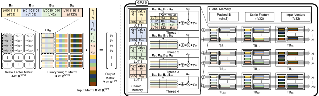</details> ●❄❅❆❇❈ ❉❊❋❍❏❑ /a242/a243/a244 /a245/a246/a247 Fig. 7. The overview of nuQmm implementation on GPUs. In this example, we assume m = 12 , n = 96 , µ = 8 , t h = 4 , l = 4 , t w = 32 , q = 1 , and g = 32 . ' ◦ ' denotes element-wise multiplication and ' · ' indicates a tensor product. - To improve parallelism, we create as many threads as possible while each thread is allowed to perform independent LUT accesses. - Binary weights accessed by a thread can share a common scaling factor such that operations related to scaling factors do not degrade the performance of a thread. - If we allocate too small resources to a thread, then LUT utilization can be low and synchronization overhead can increase. As such, we need to optimize thread configurations empirically. For the sake of simplicity, we formulate the proposed group-wise quantized matrix multiplication as y = ∑ q i =1 ( A i ◦ ( B i · x )) , where A is an ( m × n ) FP32 scaling matrix, B is an ( m × n ) FP32 binary matrix, x is an FP32 input vector of size n , and the operator ◦ indicates elementwise multiplication. Note that in real situations, the memory footprint of A is reduced by g since every g weights share a scaling factor. - a) Overall Architecture: For nuQmm, we assign l number of LUTs to a thread block (TB) of GPU. Then, the size of submatrix of A and B allocated to each TB becomes ( t h × t w ) when t w = l × µ . Small t h can increase the number of available threads while large t h enhances LUT utilization inside a TB. Thus, t h is empirically determined (2048 is a practical number for large-scale LMs). Note that the amount of resources allocated to each TB is small enough such that multiple TBs can share a scaling factor as long as g is larger than l × µ . The overall nuQmm implementation scheme on GPUs is presented in Fig. 7 when we assume µ = 8 , l = 4 , t w = 32 , t h = 4 , q = 1 , and g = 32 . For q > 1 , the entire process of Fig. 7 can be iterated q times while intermediate results are accumulated. - b) Detailed Implementation: Each TB first conducts precomputation using partial x values assigned in order to fill up the l number of LUTs. Then l LUTs can be shared by all threads inside a TB (so as to mitigate costly global memory accesses) and multiple rows of a submatrix of B can be processed by multiple threads (so as to improve throughput). TABLE III COMPARISON BETWEEN FP32 GEMM IN CUBLAS AND NUQMM. AN ( m × n ) MATRIX IS MULTIPLIED BY ( n × 1) MATRIX AS AN SINGLE-BATCH OPERATION. | m = n | q | Memory (MB) | Memory (MB) | Latency ( µ s) | Latency ( µ s) | |---------|---------|---------------|---------------------------------------------------------------|------------------|--------------------------------------------------------------| | | | cuBLAS | nuQmm ( Reduction ) | cuBLAS | nuQmm ( Speed up ) | | 2048 | 2 3 4 5 | 16.78 | 1.06 ( x15.9 ) 1.58 ( x10.6 ) 2.11 ( x8.0 ) 2.63 ( x6.4 ) | 30.99 | 9.54 ( x3.2 ) 10.23 ( x3.0 ) 10.93 ( x2.8 ) 11.43 ( x2.7 ) | | 4096 | 2 3 4 5 | 67.11 | 4.21 ( x15.9 ) 6.31 ( x10.6 ) 8.40 ( x8.0 ) 10.50 ( x6.4 ) | 88.01 | 15.17 ( x5.8 ) 17.35 ( x5.1 ) 20.98 ( x4.2 ) 23.48 ( x3.7 ) | | 8192 | 2 3 4 5 | 268.44 | 16.81 ( x16.0 ) 25.20 ( x10.7 ) 33.59 ( x8.0 ) 41.98 ( x6.4 ) | 313.22 | 37.65 ( x8.3 ) 44.94 ( x7.0 ) 52.06 ( x6.0 ) 60.19 ( x5.2 ) | | 12288 | 2 3 4 5 | 603.98 | 37.80 ( x16.0 ) 56.67 ( x10.7 ) 75.55 ( x8.0 ) 94.42 ( x6.4 ) | 697.85 | 73.45 ( x9.5 ) 84.45 ( x8.3 ) 99.93 ( x7.0 ) 117.67 ( x5.9 ) | When threads finish retrieving and summing LUT values, scaling factors are fetched (only once for each thread) and multiplied to produce partial outputs. Finally, n l × µ partial outputs are accumulated across TBs (through atomicAdd operations, as illustrated in Fig. 7) to generate the final outputs. LUTs are stored in shared memory inside GPU and the shared memory presents high bandwidth (e.g., 17TB/s for RTX3090). Thus, high memory accesses for LUTs (while multiple FLOPs can be replaced with one LUT access) enable fast matrix computations. As for memory size of LUTs, only 1KB is required for every 8 hidden dimensions and the shared memory size is more than a few megabytes (e.g., 10MB for RTX-3090 with 128KB per SM and 82 SMs available). Thus, the whole LUTs can be safely stored in shared memory. To illustrate, the hidden dimension can be up to 80,000 for RTX3090 while 16,384 is the hidden dimension for GPT-3 175B. Table III compares memory footprint and latency between conventional FP32 GEMM kernel in cuBLAS library and our /a116 <details> <summary>Image 8 Details</summary>  ### Visual Description ## Line Chart: Normalized Latency vs. g ### Overview The chart illustrates the relationship between normalized latency and the variable `g` for three distinct system configurations defined by `m = n` values (4096, 8192, 12288). All three data series exhibit a decreasing trend in normalized latency as `g` increases, with convergence observed at higher `g` values. ### Components/Axes - **Y-Axis**: Normalized Latency (scale: 1 to 4, linear increments of 1). - **X-Axis**: `g` (values: 8, 16, 32, 64, 128, 256, 512, 1024). - **Legend**: - Orange: `m = n = 4096` - Blue: `m = n = 8192` - Green: `m = n = 12288` - **Legend Placement**: Top-right corner of the chart. ### Detailed Analysis 1. **Orange Series (`m = n = 4096`)**: - Starts at ~2.8 (g=8) and decreases sharply to ~1.0 by g=1024. - Steepest initial decline among all series. - Data points: (8, 2.8), (16, 1.8), (32, 1.4), (64, 1.2), (128, 1.1), (256, 1.05), (512, 1.02), (1024, 1.0). 2. **Blue Series (`m = n = 8192`)**: - Begins at ~3.8 (g=8) and declines gradually to ~1.0 by g=1024. - Intermediate rate of decrease compared to orange and green. - Data points: (8, 3.8), (16, 2.3), (32, 1.7), (64, 1.3), (128, 1.15), (256, 1.08), (512, 1.03), (1024, 1.0). 3. **Green Series (`m = n = 12288`)**: - Highest initial latency (~4.2 at g=8) but converges to ~1.0 by g=1024. - Slowest rate of decline, maintaining higher latency longer than other series. - Data points: (8, 4.2), (16, 2.5), (32, 1.9), (64, 1.4), (128, 1.2), (256, 1.1), (512, 1.05), (1024, 1.0). ### Key Observations - **Convergence**: All three series converge to ~1.0 normalized latency at `g = 1024`, suggesting diminishing returns in latency reduction beyond this point. - **Initial Disparity**: Larger `m = n` values (green > blue > orange) start with higher latency but follow similar trajectories at higher `g`. - **Rate of Decline**: Orange series (`m = n = 4096`) exhibits the fastest initial reduction in latency, while green (`m = n = 12288`) decreases most slowly. ### Interpretation The chart demonstrates that normalized latency decreases with increasing `g` across all configurations. Larger `m = n` values (e.g., 12288) exhibit higher baseline latency but show diminishing sensitivity to `g` compared to smaller configurations. This implies that system performance (latency) is more strongly influenced by `g` than by `m = n` once `g` exceeds ~128. The convergence at `g = 1024` suggests that system optimization efforts targeting `g` may yield uniform benefits regardless of `m = n` scale, though larger configurations require higher initial resource allocation to achieve baseline performance. 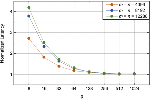</details> ✉ ✈ ✇ ① ② ③ ④ ⑤ Fig. 8. Normalized matrix multiplication latency when a ( m × n ) weight matrix is quantized by ( q =4) bits with different g values. ➆ <details> <summary>Image 9 Details</summary>  ### Visual Description ## Line Chart: Latency vs Compression Ratio ### Overview The chart illustrates the relationship between compression ratio (x-axis) and latency (y-axis) for five different configurations labeled q=2 to q=6. Latency decreases as compression ratio increases, with all configurations converging at lower latency values at higher compression ratios. ### Components/Axes - **X-axis (Compression Ratio)**: Ranges from 0 to 16 in increments of 2. Labeled "Compression Ratio." - **Y-axis (Latency)**: Ranges from 0.1 to 0.7 milliseconds (ms) in increments of 0.1. Labeled "Latency (ms)." - **Legend**: Located in the top-right corner. Colors and symbols: - q=2: Black square - q=3: Orange circle - q=4: Yellow triangle - q=5: Blue triangle - q=6: Green diamond - **Grid**: Light gray grid lines with darker axes. ### Detailed Analysis - **q=2 (Black Square)**: Starts at ~0.6 ms at compression ratio 1, decreases to ~0.1 ms by compression ratio 10, and stabilizes near 0.1 ms. - **q=3 (Orange Circle)**: Begins at ~0.55 ms at compression ratio 1, drops to ~0.1 ms by compression ratio 8, and remains flat. - **q=4 (Yellow Triangle)**: Starts at ~0.5 ms at compression ratio 1, decreases to ~0.1 ms by compression ratio 6, and stabilizes. - **q=5 (Blue Triangle)**: Initiates at ~0.45 ms at compression ratio 1, drops to ~0.1 ms by compression ratio 4, and remains constant. - **q=6 (Green Diamond)**: Begins at ~0.4 ms at compression ratio 1, decreases to ~0.1 ms by compression ratio 2, and stabilizes. ### Key Observations 1. **Inverse Relationship**: All configurations show latency decreasing as compression ratio increases. 2. **Convergence**: By compression ratio 10–12, all q values converge to ~0.1 ms latency. 3. **Initial Variability**: Higher q values (e.g., q=6) start with lower latency at compression ratio 1 compared to lower q values (e.g., q=2). 4. **Stability**: After compression ratio 10, latency plateaus for all configurations. ### Interpretation The data suggests that increasing compression ratio significantly reduces latency across all configurations, with diminishing returns beyond a compression ratio of 10. The convergence of lines at low latency values implies that further compression offers minimal latency benefits. The initial differences in latency between q values may reflect inherent configuration efficiencies (e.g., q=6 being optimized for lower latency at low compression ratios). This trend is critical for optimizing performance in systems where latency and compression trade-offs are prioritized. </details> ➃ ➄ ➅ ➇ ➈ ➉ ➊ ➋ Fig. 9. Relationship between latency and compression ratio when nuQmm performs quantized matrix multiplications with m = 12288 and various ( q , g ) pairs. proposed nuQmm. For experiments, we multiply an ( m × n ) matrix (that can be quantized by q bits) and an ( n × 1) matrix using a single Nvidia 3090 GPU with CUDA 11.5. We can observe that the memory size and execution time required for both cuBLAS and nuQmm increase with larger m (and q for nuQmm). It is clear that the relative reduction of memory footprint and latency by nuQmm increases when a larger weight matrix is employed. Such observation can be partly explained by the fact that kernel launch overhead appears as a performance bottleneck for small matrices (such as m = 2048 ). Thus, the merits of nuQmm would be outstanding as larger-scale generative LMs are introduced. To examine latency variance of nuQmm on group size g , we perform matrix multiplications (using an ( m × n ) matrix and an ( n × 1) matrix) when g values vary. In Fig. 8, for each m (= n ) selection, matrix multiplication latency of different g is compared with that of row-wise (i.e., g = n ) BCQ format. Interestingly, when g > 64 , group-wise nuQmm is as fast as row-wise nuQmm regardless of m in Fig 8. In other words, ➌ ➍ ⑥ ⑦ ⑧ ⑨ ⑩ ❶ ❷ ❸ ❹ ❺❻❼❽ a reasonably large g (such as 256 and 512) can result in fast nuQmm while accuracy improvement by group-wise is substantial as can be seen in Fig. 5. To understand the underlying mechanisms in Fig. 8, we analyze memory footprint of nuQmm because single-batch operations are basically memory-bound such that latency is proportional to memory footprint. Let S b and S α represent space complexity of binary weights and scaling factors, respectively. Then the overall space complexity S can be described as $$\begin{array}{ll} S = S _ { 0 } + S _ { a } & = O \left( 1 \cdot m \cdot n - q ^ { n } + 3 2 \cdot m \cdot \frac { n } { q } \right) \\ & = O \left( m \cdot n \cdot \frac { n } { q } \right) . 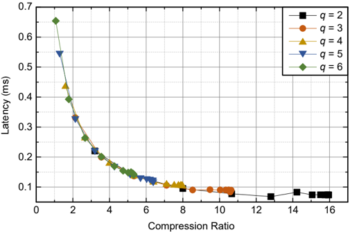\end{array}$$ As a consequence, if g /greatermuch 32 , S can be independent of g and approximated to be O ( m · n · q ) . To verify our claim that latency of nuQmm is proportional to memory footprint (when running single-batch operations), we explore various ( q, g ) pairs and compression ratios correspondingly, and measure matrix multiplication latency when m = 12288 as shown in Fig. 9. It can be noticed that the additional search parameter g allows a fine-grained search space of compression ratio that is not available by q alone. Across all available compression ratios in Fig. 9, latency is a function of compression ratio. For instance, if two different pairs ( q 1 , g 1 ) and ( q 2 , g 2 ) exhibit a similar memory footprint, then we can expect similar latency by nuQmm. ## D. Comparison with Tensor Parallelism (of Full-Precision) Since the model size is rapidly increasing in order to empower language models to improve accuracy on various tasks, computing systems are scaled up with a growing number of computation units and memory capacity. Note that for highly parallel computing systems, such as GPUs, high memory bandwidth is essential to feed lots of arithmetic units so as to maintain high resource utilization. The main memory system of GPUs, hence, is inclined to focus on high bandwidth instead of large capacity. Correspondingly, even though new innovative memory architectures (e.g., HBM [39]) are proposed, the maximum memory capacity for a single GPU is still limited up to a few tens of gigabytes [16]. Such limited GPU's memory capacity derived various parallelism ideas to partition a large-scale LM over multiple GPUs [13], [14]. In this work, we consider tensor parallelism that can split matrix multiplications over multiple GPUs, which is useful for both training and inference. Note that even though tensor parallelism can generate smaller sub-tasks that can be executed simultaneously, synchronization and GPT-to-GPU communication overhead are additionally induced. Our new BCQ format and nuQmm can reduce the model size with low latency such that the overhead of tensor parallelism can be alleviated. For a comparison between nuQmm and cuBLAS, we measure the latency of completing a large matrix multiplication as TABLE IV PROFILING RESULTS OF MATRIX MULTIPLICATIONS (WITH AN ( m × m ) MATRIX AND AN ( m × 1) MATRIX). FOR NUQMM, g = m AND q IS 2 OR 4. | Type | GPUs | m | Comput. Ratio ( % ) | Comm. Ratio ( % ) | Speed up | GPU Util. ( % ) | Memory Util. ( % ) | Average Power (W) | Total Energy (mJ) | Normalized Energy | |-----------------|--------|-------|-----------------------|---------------------|------------|-------------------|----------------------|---------------------|---------------------|---------------------| | cuBLAS | 1 | 8192 | 100 | 0 | 1 | 96.67 | 100 | 318.33 | 99.8 | 1 | | cuBLAS | 2 | 8192 | 84.55 | 15.45 | 1.54 | 88.06 | 92.46 | 321.06 | 130.77 | 1.31 | | cuBLAS | 4 | 8192 | 68.84 | 31.16 | 1.95 | 72.82 | 59.73 | 260.78 | 168.14 | 1.68 | | cuBLAS | 8 | 8192 | 55.23 | 44.77 | 1.73 | 55.25 | 26.92 | 197.01 | 286.5 | 2.87 | | nuQmm ( q = 2 ) | 1 | 8192 | 100 | 0 | 8.33 | 85.85 | 69.9 | 333.78 | 12.57 | 0.13 | | nuQmm ( q = 4 ) | 1 | 8192 | 100 | 0 | 5.9 | 90.85 | 82.89 | 331.97 | 17.64 | 0.18 | | cuBLAS | 1 | 12288 | 100 | 0 | 1 | 97.37 | 100 | 317.9 | 221.59 | 1 | | cuBLAS | 2 | 12288 | 90.44 | 9.56 | 1.76 | 93.38 | 99.79 | 320.57 | 254.41 | 1.15 | | cuBLAS | 4 | 12288 | 80.56 | 19.44 | 2.46 | 83.29 | 81.4 | 310.75 | 351.49 | 1.59 | | cuBLAS | 8 | 12288 | 61.65 | 38.35 | 2.98 | 64.59 | 45.33 | 239.83 | 448.29 | 2.02 | | nuQmm ( q = 2 ) | 1 | 12288 | 100 | 0 | 12.21 | 91.36 | 91.35 | 331.21 | 18.91 | 0.09 | | nuQmm ( q = 4 ) | 1 | 12288 | 100 | 0 | 6.89 | 95.02 | 99.57 | 327.07 | 33.1 | 0.15 | | cuBLAS | 1 | 16384 | 100 | 0 | 1 | 98.16 | 100 | 317.83 | 387.72 | 1 | | cuBLAS | 2 | 16384 | 93.15 | 6.85 | 1.77 | 94.6 | 100 | 321.13 | 435.48 | 1.12 | | cuBLAS | 4 | 16384 | 84.04 | 15.96 | 3.06 | 89.86 | 94.4 | 319.52 | 510.66 | 1.32 | | cuBLAS | 8 | 16384 | 69.01 | 30.99 | 3.89 | 72.83 | 60.33 | 263.67 | 663.54 | 1.71 | | nuQmm ( q = 2 ) | 1 | 16384 | 100 | 0 | 13.41 | 93.92 | 99.2 | 329.24 | 29.95 | 0.08 | | nuQmm ( q = 4 ) | 1 | 16384 | 100 | 0 | 7.43 | 96.94 | 100 | 327.98 | 53.88 | 0.14 | 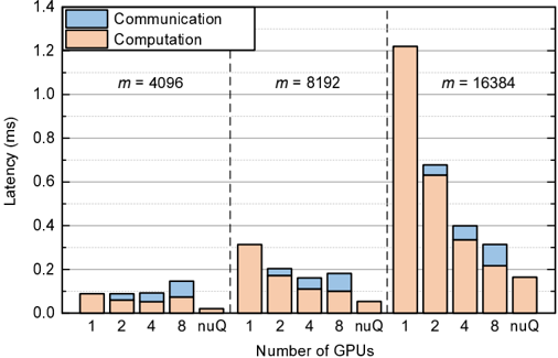shown in Fig. 10. We assume that we multiply an ( m × m ) matrix and an ( m × 1 ) matrix (as a single-batch operation to run inference of generation steps in Fig. 1) when m can be 4096, 8192, or 16384. For conventional full-precision (FP32) cuBLAS [11], one to eight GPUs serve tensor parallelism through NCCL library [16] to communicate via PCIe 4.0. When nuQmm is applied (with only one GPU), q is given as 4 and g is the same as m 5 . From Fig. 10, we observe the following: 1) for cuBLAS, more GPUs with tensor parallelism can reduce the overall computation latency while communication latency increases, 2) tensor parallelism is more effective with larger m , and 3) for all three m configurations, nuQmm is faster than cuBLAS even 8 GPUs are employed. Note that if m is small, then communication latency (including GPU-to-GPU communication and synchronization across GPUs) cannot be ignored. As such, latency improvement by tensor parallelism is a sub-linear function of the number of GPUs (for any m ) such that certain configurations of tensor parallelism may even harm the overall inference latency (while the cost of inference system increases due to more GPUs). In the case of nuQmm, the requirement for tensor parallelism can be eliminated (or alleviated) due to reduced model size. As a result, nuQmm can reduce both latency and system design cost of inference. Table IV is a summary of profiling results of matrix multiplications performed by using cuBLAS (with tensor parallelism) or nuQmm (with one GPU). In this work, GPU power and other metrics are collected by using nvidia-smi utility [40], [41]. Again, an ( m × m ) matrix is multiplied by an ( m × 1 ) matrix while we select m to be 8192, 12288 (used for GPT-3 175B), or 16384. For Table IV, we include the case of q = 2 for nuQmm (with g = m ) as 2-bit quantization for the Transformer is reported to be feasible by quantization-aware training along with BCQ format [30]. We notice that throughout all m configurations, increasing 5 As shown in Fig. 8, unless g is too small, g does not affect latency noticeably. Thus, we show row-wise quantization results in this section. GPUs for cuBLAS with tensor parallelism brings about a higher reduction in GPU utilization, memory utilization, and latency ratio of computations. As evidenced by the increase in the latency ratio of communication, such reductions in utilization indicate that some GPUs can be temporarily idle until all GPUs are synchronized. Accordingly, the amount of speed-up that can be obtained by tensor parallelism is a lot smaller than the number of GPUs. As a result, cuBLAS with more GPUs causes increased energy consumption for matrix multiplications. On the other hand, nuQmm (with one GPU) can offer high speed-up (that cannot be achieved by tensor parallelism) while retaining high GPU/memory utilization. Combining low latency and a reduced number of GPUs, thus, nuQmm saves energy consumption for matrix multiplications significantly. For example, when m = 12288 , nuQmm (with q = 2 ) achieves 11 . 7 × energy reduction and 12 . 2 × speed-up compared to cuBLAS with one GPU. ## IV. 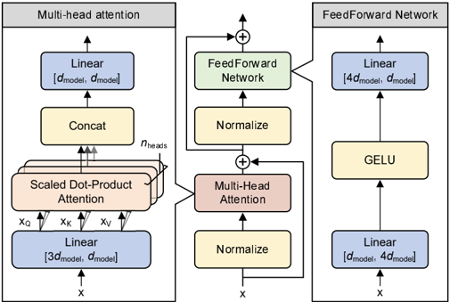EXPERIMENTAL RESULTS ON GPT-3 175B In this section, we apply nuQmm to major matrix multiplications in GPT-3 175GB [6] (chosen as a representative largescale LM) and estimate speed-up and energy reduction. GPT3 follows the structure of the Transformer [5] that consists of identical layers. Assuming that m is the hidden size (i.e., d model ), each layer has multi-head attention and feed-forward network as shown in Fig. 11 and includes 4 major linear computations of higher time complexity (than the other nonlinear operations) for which we multiply a ( m × 1 ) activation matrix and the following 4 matrices: - ( m × m ) matrix for attention output - ( 3 m × m ) matrix for key, query, and value of attention - ( m × 4 m ) matrix for the first feed-forward sub-layer - ( 4 m × m ) matrix for the second feed-forward sub-layer Since all layers of the Transformers have identical structures and matrix multiplications dominate the entire inference latency [30], we can successfully approximate the overall impact ➺ <details> <summary>Image 10 Details</summary>  ### Visual Description ## Bar Chart: Latency Comparison Across GPU Configurations and Matrix Sizes ### Overview The chart compares communication and computation latency (in milliseconds) for three matrix sizes (m = 4096, 8192, 16384) across varying numbers of GPUs (1, 2, 4, 8) and a "nuQ" configuration. Latency is split into two components: communication (blue) and computation (orange). Vertical dashed lines separate the three matrix size categories. ### Components/Axes - **X-axis**: Number of GPUs (1, 2, 4, 8, "nuQ"). Labels are centered below each bar group. - **Y-axis**: Latency (ms), ranging from 0.0 to 1.4 ms in 0.2 ms increments. - **Legend**: Top-left corner, with blue representing "Communication" and orange representing "Computation." - **Matrix Size Labels**: "m = 4096" (left), "m = 8192" (middle), "m = 16384" (right), positioned above their respective sections. ### Detailed Analysis #### Communication Latency (Blue) - **m = 4096**: - 1 GPU: ~0.05 ms - 2 GPUs: ~0.06 ms - 4 GPUs: ~0.08 ms - 8 GPUs: ~0.12 ms - **m = 8192**: - 1 GPU: ~0.15 ms - 2 GPUs: ~0.18 ms - 4 GPUs: ~0.20 ms - 8 GPUs: ~0.25 ms - **m = 16384**: - 1 GPU: ~0.30 ms - 2 GPUs: ~0.35 ms - 4 GPUs: ~0.40 ms - 8 GPUs: ~0.45 ms - **nuQ**: No communication latency (no blue bars). #### Computation Latency (Orange) - **m = 4096**: - 1 GPU: ~0.03 ms - 2 GPUs: ~0.04 ms - 4 GPUs: ~0.07 ms - 8 GPUs: ~0.08 ms - nuQ: ~0.02 ms - **m = 8192**: - 1 GPU: ~0.10 ms - 2 GPUs: ~0.12 ms - 4 GPUs: ~0.15 ms - 8 GPUs: ~0.20 ms - nuQ: ~0.05 ms - **m = 16384**: - 1 GPU: ~0.60 ms - 2 GPUs: ~0.65 ms - 4 GPUs: ~0.70 ms - 8 GPUs: ~0.75 ms - nuQ: ~0.15 ms ### Key Observations 1. **Computation Dominates**: Computation latency consistently exceeds communication latency across all matrix sizes and GPU counts. 2. **Scaling Trends**: - For smaller matrices (m = 4096), latency increases modestly with more GPUs. - For larger matrices (m = 16384), latency spikes dramatically, especially for computation. 3. **nuQ Exception**: The "nuQ" configuration shows significantly lower computation latency (e.g., ~0.15 ms for m = 16384 vs. ~0.75 ms for 8 GPUs). 4. **Communication Scaling**: Communication latency increases with matrix size but remains relatively stable per GPU count (e.g., ~0.45 ms for 8 GPUs in m = 16384 vs. ~0.12 ms for 8 GPUs in m = 4096). ### Interpretation - **Computation Bottleneck**: The data highlights computation as the primary latency driver, particularly for large matrices. Adding GPUs reduces per-GPU computation time but does not eliminate the inherent complexity of larger matrices. - **nuQ Optimization**: The "nuQ" configuration suggests a specialized setup (e.g., no inter-GPU communication overhead) that drastically reduces computation latency, likely by avoiding synchronization delays. - **Scalability Limits**: While increasing GPUs improves performance, diminishing returns are evident for large matrices (e.g., 8 GPUs for m = 16384 only reduces computation latency to ~0.75 ms from ~0.60 ms for 1 GPU). - **Communication-Computation Balance**: For smaller matrices, communication latency is a smaller fraction of total latency, but this ratio worsens for larger matrices (e.g., m = 16384: communication = 0.45 ms, computation = 0.75 ms → 60% of total latency). ### Spatial Grounding & Verification - **Legend Alignment**: Blue bars (communication) and orange bars (computation) match the legend colors exactly. - **Trend Verification**: - Communication latency slopes upward with matrix size but plateaus per GPU count. - Computation latency slopes upward steeply for larger matrices, confirming its dominance. - **Outliers**: The "nuQ" configuration deviates from the GPU-count trend, suggesting a non-standard optimization. ### Conclusion The chart demonstrates that computation latency scales non-linearly with matrix size, while communication latency grows linearly. The "nuQ" configuration offers a potential pathway to mitigate computation bottlenecks, though its applicability depends on the specific hardware/software constraints. </details> ➻ ➼ ➽ ➾ ➚ ➪ ➶ ➹ Fig. 10. Latency comparison between full-precision cuBLAS and nuQmm. We multiply an ( m × m ) matrix and ( m × 1) matrix (for single-batch inference). For cuBLAS, tensor parallelism is utilized with up to 8 GPUs. For nuQmm, q and g are 4 and m , respectively. <details> <summary>Image 11 Details</summary>  ### Visual Description ## Diagram: Transformer Block Architecture ### Overview The image depicts a technical diagram of a transformer block architecture, illustrating the flow of data through multi-head attention mechanisms and feedforward networks. The diagram uses color-coded blocks to represent different computational steps, with arrows indicating data flow. ### Components/Axes 1. **Multi-head Attention Block (Left Section)** - **Linear Layers**: - Input: `[3d_model, d_model]` → Output: `[d_model, d_model]` - Output: `[d_model, d_model]` → Output: `[d_model, d_model]` - **Concat**: Combines outputs from multiple attention heads. - **Scaled Dot-Product Attention**: - Inputs: `x_q` (queries), `x_k` (keys), `x_v` (values). - Dimensions: `[d_model, d_model]` for all inputs. - **Normalize**: Applied after attention computation. - **n_heads**: Number of attention heads (not quantified numerically). 2. **FeedForward Network (Right Section)** - **Linear Layers**: - Input: `[d_model, 4d_model]` → Output: `[4d_model, d_model]`. - **GELU Activation**: Applied after the first linear layer. - **Normalize**: Applied after the GELU activation. 3. **Residual Connections**: - "+" symbols indicate residual connections between blocks (e.g., input + output of attention/feedforward). ### Detailed Analysis - **Multi-head Attention Flow**: 1. Input `x` is linearly transformed into queries (`x_q`), keys (`x_k`), and values (`x_v`). 2. Scaled dot-product attention computes relationships between queries and keys, then applies softmax to weight values. 3. Outputs from all attention heads are concatenated and linearly projected back to `[d_model, d_model]`. 4. Normalization stabilizes the output. - **FeedForward Network Flow**: 1. Input `x` is linearly expanded to `[4d_model]` using GELU activation for non-linearity. 2. A second linear layer projects the output back to `[d_model]`. 3. Normalization is applied to stabilize gradients. - **Residual Connections**: - Data is added to the input of each block (e.g., `x + attention_output`), enabling deeper networks by mitigating vanishing gradients. ### Key Observations - **Dimensionality Changes**: - Attention heads reduce dimensionality via linear projections (e.g., `[3d_model, d_model]` → `[d_model, d_model]`). - Feedforward network expands and contracts dimensions (`[d_model, 4d_model]` → `[4d_model, d_model]`). - **Activation Functions**: - GELU (Gaussian Error Linear Unit) introduces non-linearity in the feedforward path. - **Normalization**: - Applied after both attention and feedforward steps to ensure stable training. ### Interpretation This diagram represents a core component of transformer models (e.g., BERT, GPT). The multi-head attention mechanism allows the model to focus on different parts of the input simultaneously, while the feedforward network adds non-linear transformations. Residual connections and normalization are critical for training deep networks by preserving gradient flow and stabilizing activations. The architecture balances computational efficiency (via attention heads) and representational power (via feedforward expansions). No numerical data or trends are present in the diagram; it focuses on structural relationships and component roles. </details> ➳➵➸ /a220/a221/a222/a223/a224/a225/a226/a227/a228/a229/a230/a231/a232 ❁❂❃❄❅❇❈❉❊❍ ■❏▲❖/a80❘❙❚❯ ❲❳❨❩❬❭❫❴❵❛❜ ❝❞❡❢❣✐❥ Fig. 11. Transformer layer incorporating multi-head attention and feedforward network performing 4 major matrix multiplications. of nuQmm on a generative LM by estimating speed-up and energy reduction using the above 4 matrix multiplications. By setting m to be hidden dimension size 12288 of GPT3 175B, Table V compares speed-up and energy reduction between cuBLAS (1 or 8 GPUs) and nuQmm ( q is 2 or 4). It should be noted that even though we include the result of FP32 cuBLAS with one GPU, the entire parameters of GPT-3 175B cannot be stored in the main memory of one GPU. Thus, multiple GPUs would be mandatory if we do not quantize GPT-3 175B. We can observe that for all matrix multiplications in Table V, nuQmm presents high performance with less energy consumption. Even though we present a few matrix configurations Table V, such matrix configurations are repeatedly presented through Transformer blocks of the same structure. Thus, Table V is useful to estimate the overall performance improvement of GPT models as m increases or nuQmm is applied. Overall, the total speed-up and energy reduction of GPT-3 175B by nuQmm (with q = 2 ) can be approximated to be 14 . 4 × and 14 . 3 × , respectively, compared ➘ ➴ TABLE V SPEED-UP AND ENERGY REDUCTION BY NUQMM ON GPT-3 175B FOR WHICH m IS SET TO BE HIDDEN DIMENSION SIZE 12288. | Layer Type (Shape) | Kernel | GPUs | q | Speed-up | Norm. Energy | |-------------------------------------|----------|--------|--------|------------|----------------| | Attention query,key,value ( 3 m,m ) | cuBLAS | 1 | (FP32) | 1 | 1 | | Attention query,key,value ( 3 m,m ) | cuBLAS | 8 | (FP32) | 4.18 | 1.65 | | Attention query,key,value ( 3 m,m ) | nuQmm | 1 | 2 | 14.29 | 0.07 | | Attention query,key,value ( 3 m,m ) | nuQmm | 1 | 4 | 7.47 | 0.14 | | Attention output ( m,m ) | cuBLAS | 1 | (FP32) | 1 | 1 | | Attention output ( m,m ) | cuBLAS | 8 | (FP32) | 3 | 2.02 | | Attention output ( m,m ) | nuQmm | 1 | 2 | 12.25 | 0.09 | | Attention output ( m,m ) | nuQmm | 1 | 4 | 6.88 | 0.15 | | FFN 1st sub-layer ( m, 4 m ) | cuBLAS | 1 | (FP32) | 1 | 1 | | FFN 1st sub-layer ( m, 4 m ) | cuBLAS | 8 | (FP32) | 5.65 | 1.38 | | | nuQmm | 1 | 2 | 15.04 | 0.07 | | | nuQmm | 1 | 4 | 7.8 | 0.13 | | FFN 2nd sub-layer ( 4 m,m ) | cuBLAS | 1 | (FP32) | 1 | 1 | | | cuBLAS | 8 | (FP32) | 4.7 | 1.47 | | | nuQmm | 1 | 2 | 14.54 | 0.07 | | | nuQmm | 1 | 4 | 7.41 | 0.14 | | Total | cuBLAS | 1 | (FP32) | 1 | 1 | | (Attention | cuBLAS | 8 | (FP32) | 4.59 | 1.53 | | + FFN) | nuQmm | 1 | 2 | 14.41 | 0.07 | | (Attention | nuQmm | 1 | 4 | 7.5 | 0.14 | to cuBLAS with 1 GPU (or 3 . 2 × and 21 . 9 × , respectively, compared to cuBLAS with 8 GPUs). In our experiments, we do not consider uniform quantization because 1) at least 8 bits are necessary for the Transformers [27], [28], [30], 2) activations need to be dynamically quantized during inference with quantization/dequantization overhead, and 3) to the best of our knowledge, uniform quantization for generative LMs has not been reported. ## V. EXTENSION OF NUQMM FOR GENERATIVE LMS In this section, we discuss additional architectural considerations for nuQmm to be extensively useful for various generative language models. ## A. Mixed Precision using nuQmm It is well known that different layers of neural networks present different sensitivity to model compression [42], [43]. For example, parameter pruning acquires various pruning rates for layers given a target global pruning rate and test accuracy [44], [45]. As such, mixed precision techniques for quantization are eligible for obtaining higher compression ratio practical techniques by assigning different quantization bits to layers while measuring accurate sensitivity of layers is complicated and computationally demanding [42], [46]. Note that since we introduce an additional parameter g (i.e., group size for scaling factors), nuQmm can offer wider search space exploration for mixed precision compared to the conventional methods allowing the number of quantization bits as the only search parameter. For experiments, we consider two sub-layers (multi-head attention and feed-forward networks) in Fig. 11 to be quantized by different quantization schemes with nuQmm. In order to facilitate efficient exploration of search space for mixed precision, we set the following constraints: 1) all matrices of Fig. 12. Mixed precision quantization results using GPT Neo 1.3B. All matrices of the same sub-layer type are quantized by the same ( q, g ) configuration. Available sets for exploring q and g are { 3 , 4 , 5 } and { 128 , 256 , 512 , 2048 } , respectively. 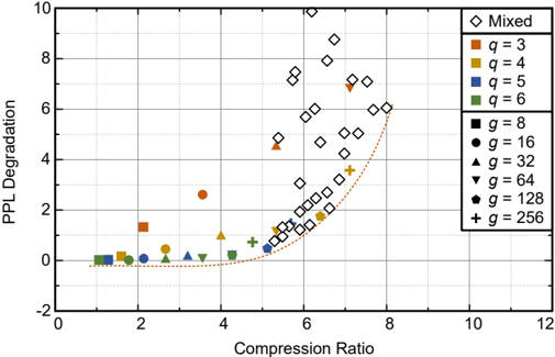<details> <summary>Image 12 Details</summary>  ### Visual Description ## Scatter Plot: PPL Degradation vs. Compression Ratio ### Overview The image is a scatter plot comparing **PPL Degradation** (y-axis) against **Compression Ratio** (x-axis). Data points are categorized by two parameters: **q** (number of categories) and **g** (model size). A dashed orange trend line indicates a general upward trend in PPL degradation as compression ratio increases. The legend on the right maps symbols and colors to specific **q** and **g** values. --- ### Components/Axes - **X-axis (Compression Ratio)**: Ranges from 0 to 12, with gridlines at integer intervals. - **Y-axis (PPL Degradation)**: Ranges from -2 to 10, with gridlines at integer intervals. - **Legend**: Located in the top-right corner. Symbols and colors represent: - **q values**: - Orange square: q = 3 - Yellow circle: q = 4 - Blue diamond: q = 5 - Green triangle: q = 6 - **g values**: - Black square: g = 8 - Black circle: g = 16 - Black triangle: g = 32 - Black inverted triangle: g = 64 - Black pentagon: g = 128 - Black plus: g = 256 - **Mixed**: White diamond (no explicit **q** or **g** label). --- ### Detailed Analysis #### Data Series Trends 1. **Mixed (White Diamonds)**: - Scattered across the plot, with concentrations at compression ratios 5–8 and PPL degradation 4–8. - Example points: (5, 5), (6, 6), (7, 7), (8, 8). 2. **q = 3 (Orange Squares)**: - Two points: (2, 1) and (4, 3). - Lower PPL degradation compared to other **q** values at similar compression ratios. 3. **q = 4 (Yellow Circles)**: - Points at (3, 0.5), (4, 1), and (5, 2). - Moderate degradation, increasing with compression ratio. 4. **q = 5 (Blue Diamonds)**: - Points at (4, 1.5), (5, 2.5), and (6, 4). - Higher degradation than **q = 3** and **q = 4** at similar compression ratios. 5. **q = 6 (Green Triangles)**: - Points at (3, 0.2), (4, 0.5), and (5, 1). - Lowest degradation among **q** values. 6. **g = 8 (Black Squares)**: - Points at (1, 0), (2, 0.5), and (3, 1). - Minimal degradation, suggesting smaller model size mitigates degradation. 7. **g = 16 (Black Circles)**: - Points at (2, 0.3), (3, 0.6), and (4, 1.2). - Slightly higher degradation than **g = 8**. 8. **g = 32 (Black Triangles)**: - Points at (3, 0.8), (4, 1.5), and (5, 2.5). - Moderate degradation, increasing with compression ratio. 9. **g = 64 (Black Inverted Triangles)**: - Points at (4, 2), (5, 3.5), and (6, 5). - Higher degradation than smaller **g** values. 10. **g = 128 (Black Pentagons)**: - Points at (5, 4), (6, 5.5), and (7, 7). - Significant degradation, especially at higher compression ratios. 11. **g = 256 (Black Plus)**: - Points at (6, 6), (7, 7.5), and (8, 9). - Highest degradation, with a steep upward trend. #### Trend Line - The dashed orange line curves upward, indicating a **non-linear relationship** between compression ratio and PPL degradation. The slope steepens as compression ratio increases, suggesting diminishing returns in compression efficiency at higher ratios. --- ### Key Observations 1. **Compression Ratio Impact**: - PPL degradation generally increases with compression ratio, but the relationship is not strictly linear. - At compression ratios >6, degradation accelerates sharply (e.g., **g = 256** at (8, 9)). 2. **q vs. g Interaction**: - Higher **q** values (e.g., q = 6) show lower degradation than lower **q** values (e.g., q = 3) at similar compression ratios. - Larger **g** values (e.g., g = 256) exhibit significantly higher degradation, implying model size exacerbates degradation. 3. **Outliers**: - The **q = 3** point at (4, 3) is an outlier, as it has higher degradation than other **q = 3** points at similar compression ratios. - The **g = 256** point at (8, 9) is the highest degradation observed, far exceeding other data points. --- ### Interpretation The plot demonstrates that **PPL degradation** is influenced by both **compression ratio** and **model size (g)**. Higher compression ratios correlate with increased degradation, but the effect is non-linear, with a steep rise at higher ratios. Larger models (higher **g**) exacerbate degradation, suggesting that compression techniques may disproportionately harm larger models. The **q** parameter (number of categories) also plays a role: lower **q** values (e.g., q = 3) show higher degradation than higher **q** values (e.g., q = 6) at similar compression ratios, indicating that simpler categorization schemes may be less robust to compression. The **Mixed** category’s variability suggests that real-world data (with mixed **q** and **g** values) experiences degradation across a wide range. This highlights the trade-off between compression efficiency and model performance, with no single optimal configuration. </details> each sub-layer type (i.e., multi-head attention or feed-forward network) across all layers are quantized by the same ( q, g ) configuration, 2) q is selected to be one of { 3 , 4 , 5 } , and 3) g is selected to be one of { 128 , 256 , 512 , 2048 } that lead to less than 10% latency overhead compared to row-wise quantization as depicted in Fig. 8. Fig. 12 shows PPL degradation of GPT Neo 1.3B quantized by mixed precision (using two ( q, g ) configurations as described above) in addition to the previous quantization results of Fig. 5 that allow only one ( q, g ) configuration across all layers. Notice that mixed precision combined with additional parameter g produces extensive trade-offs between PPL degradation and compression ratio. Due to our selected ranges for q and g , we extract numerous ( q, g ) pairs enabling high compression ratio with reasonable PPL degradation in Fig. 12. Further optimal points would be obtainable by fine-grained mixed precision with more diversified ( q, g ) configurations for layers and matrices at the cost of additional evaluation time. ## B. Context Processing using Quantized Weights As we discussed, inference of generative LMs can be separated into the summarization stage (using input context) and the generation stage as shown in Fig. 2. Note that even though the same weights can be applied to both summarization and generation, those two processes require different batch sizes. As for summarization, since tokens for input context are already provided, multiple tokens can be fed into the Transformer to improve explicit parallelism. On the other hand, the generation stage is fundamentally processed by single-batch operations because of autoregressive properties. In other words, inference of generative LMs is basically supposed to support two potentially conflicting operations, namely, compute-bound context process with high parallelism and memory-bound generation process with low parallelism. 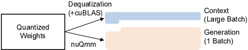Because nuQmm is specifically designed for single-batch matrix multiplications, the context process can be better performed by conventional kernels with parallel computing ❻❼❽❾❿➀➁➂➃➄➅➆➇ <details> <summary>Image 13 Details</summary>  ### Visual Description ## Diagram: Quantized Weights Processing Flowchart ### Overview The diagram illustrates a two-pathway processing flow originating from "Quantized Weights," splitting into "Dequatization (+cuBLAS)" and "nuQmm." Each pathway feeds into distinct output stages: "Context (Large Batch)" and "Generation (1 Batch)." ### Components/Axes - **Left Section**: - **Box**: "Quantized Weights" (source node). - **Arrows**: - Top arrow labeled "Dequatization (+cuBLAS)" (blue). - Bottom arrow labeled "nuQmm" (orange). - **Right Section**: - **Top Bar**: "Context (Large Batch)" (blue, matching the top arrow). - **Bottom Bar**: "Generation (1 Batch)" (orange, matching the bottom arrow). ### Detailed Analysis - **Quantized Weights**: Central starting point, feeding into two parallel processes. - **Dequatization (+cuBLAS)**: - Process name combines "Dequatization" with the cuBLAS library (NVIDIA's GPU-accelerated BLAS implementation). - Outputs to "Context (Large Batch)," implying optimization for high-throughput scenarios. - **nuQmm**: - Likely a specialized quantization method (abbreviated from "nuQuantized Matrix Multiplication"). - Outputs to "Generation (1 Batch)," suggesting single-batch processing for targeted tasks. ### Key Observations 1. **Batch Size Differentiation**: - "Context" uses a large batch, while "Generation" uses a single batch. - This implies resource allocation trade-offs: larger batches for efficiency vs. smaller batches for precision. 2. **Library Integration**: - cuBLAS integration in the "Dequatization" path highlights GPU acceleration for scalability. 3. **Pathway Divergence**: - The split suggests architectural choices for balancing speed and accuracy in different use cases. ### Interpretation The diagram represents an optimized workflow for deploying quantized neural network models. The "Dequatization (+cuBLAS)" path prioritizes throughput for large-scale context processing (e.g., real-time inference on GPUs), while "nuQmm" targets precision in single-batch generation tasks (e.g., fine-tuning or specialized inference). The use of cuBLAS indicates reliance on hardware acceleration, whereas "nuQmm" may represent a custom or lightweight quantization strategy. This bifurcation reflects a design philosophy where different quantization methods and batch strategies are tailored to specific computational demands. **Note**: No numerical data or trends are present; the diagram focuses on architectural relationships and process flow. </details> ➈➉➊➋➌➍➎➏➐ Fig. 13. Our proposed strategy to support both context process and generation process using quantized weight with BCQ format. resources (such as Tensor Cores of Nvidia [31]). As such, we propose our inference strategy as shown in Fig. 13. Quantized weights are stored in memory in the form of BCQ and then 1) dequantized to conduct full-precision cuBLAS matrix multiplications for context process or 2) used as inputs of nuQmm for the generation process. The rationale behind our approach is as follows: - It is necessary to quantize weights even for the context process. Otherwise, the effort to save memory by nuQmm would be worthless. - Dequantization overhead (in latency) becomes ignorable as more tokens are utilized for context process and/or generation process. - If input context gets longer, then the latency of cuBLAS matrix multiplications is a lot higher than that of dequantization (due to higher time complexity). - As target tasks require more tokens to be generated, the generation stage would dominate inference latency (and then, the latency of the entire context process including dequantization can be negligible). Few-shot learning or in-context learning techniques first introduced in GPT-3 [6] intentionally require a small number of tokens for context. ## VI. DISCUSSION In this paper, we consider the FP32 format as a baseline for various comparisons with the BCQ format. Admittedly, low-precision formats are actively studied because well-trained neural networks (with proper regularization) can be robust to various noise sources. As an example, BFLOAT16 [47] has 16 bits to represent a parameter, and thus, saves memory footprint and area overhead of arithmetic units compared to FP32. Recently, large-scale generative models (e.g., [6], [9], [13]) are developed by mixing BFLOAT16 and FP32. Specifically, BFLOAT16 is selected for major matrix multiplications while FP32 is utilized to perform various non-linear operations (such as normalization layers, SoftMAX, and activation functions). Compared to FP32, BFLOAT16 can halve memory bandwidth and offer double peak performance. Thus, our estimated speedup and energy savings by nuQmm can be roughly reduced by 50% while such improvements are still significant. For our experiments, we measured the accuracy of quantized models by performing a post-training quantization method for fast design exploration of nuQmm. There are several ways to further improve accuracy and/or compression ratio. For example, quantization-aware training for Transformers [30] is reported to save additional 1 or 2 quantization bits at the cost of training time with hyper-parameter tuning. In particular to self-supervised language models, fine-tuning techniques (e.g., LoRA [48]) using a small dataset can be a potentially economic choice to improve accuracy after posttraining quantization. Applying nuQmm to such advanced quantization techniques is left as future works. Pre-trained extreme-scale language models (e.g., GPT-3 (175B) [6], HyperCLOVA (204B) [8], and Megatron Turing NLG (530B) [10]) are usually not publicly available. Thus, in this work, our detailed analysis of group-wise quantization and nuQmm is limited to relatively smaller models (such as GPT Neo). In the case of GPT-3 175B, since it is not feasible to find q for reasonable model accuracy without a pre-trained model, we assumed q = 2 or q = 4 to estimate speed-up and energy consumptions of major matrix multiplications based on the reports that larger neural networks can be quantized by a smaller number of quantization bits [21], [49]. The parameter pruning technique is a promising complement to parameter quantization in order to further compress neural networks [43], [50]. When parameters identified as unimportant are removed first, then quantization can be performed with a reduced number of parameters. Then, the number of quantization bits can also be reduced along with a smaller quantization error [51]. Both fine-grained pruning and structured pruning are investigated because of trade-offs between compression ratio and the regularity of memory access patterns [12], [52]. Exploring pruning techniques to integrate nuQmm with proper sparse representation (to be practical with GPUs or CPUs) would be interesting. ## VII. CONCLUSION Generative language models, such as GPT-3 175B, are attracting attention due to their generation capability on various complicated tasks. It is widely expected that the growth rate in parameter size would be exponential to follow scaling laws in natural language processing. The inference speed, however, is a serious concern not only because of parameter size increase but also because of autoregressive operations associated with single-batch operation. Thus, conventional matrix multiplication using cuBLAS leads to low utilization of GPUs and low performance during the running of the generation stage of the Transformer decoder. To improve the inference speed of large-scale generative models, in this paper, we proposed a new group-wise binarycoding quantization format and a dedicated matrix multiplication kernel nuQmm. By introducing a new hyper-parameter, group size, it is possible to explore a wider compression ratio such that conventional row-wise quantization is replaced with our group-wise quantization. Then, LUT-based matrix multiplication enables computations with quantized weights without a special conversion process. As such, our nuQmm can exploit both low latency and reduced memory footprint. nuQmm is especially superior to tensor parallelism that is required if a model size is too big to be accommodated in a single GPU. Combining low latency and a reduced number of GPUs, inference of GPT-3 175B can be performed with significantly reduced energy consumption. We also discussed additional considerations of nuQmm such as mixed precision and context processing. ## REFERENCES - [1] J. Devlin, M.-W. Chang, K. Lee, and K. Toutanova, 'BERT: Pretraining of deep bidirectional transformers for language understanding,' in Proceedings of the 2019 Conference of the North American Chapter of the Association for Computational Linguistics: Human Language Technologies, Volume 1 (Long and Short Papers) , 2019, pp. 4171-4186. - [2] W. Hu, B. Liu, J. Gomes, M. Zitnik, P. Liang, V. Pande, and J. Leskovec, 'Strategies for pre-training graph neural networks,' in International Conference on Learning Representations , 2020. - [3] A. Baevski, Y. Zhou, A. Mohamed, and M. Auli, 'Wav2vec 2.0: A framework for self-supervised learning of speech representations,' in Advances in Neural Information Processing Systems , vol. 33, 2020, pp. 12 449-12 460. - [4] T. Chen, S. Kornblith, M. Norouzi, and G. Hinton, 'A simple framework for contrastive learning of visual representations,' in International conference on machine learning . PMLR, 2020, pp. 1597-1607. - [5] A. Vaswani, N. Shazeer, N. Parmar, J. Uszkoreit, L. Jones, A. N. Gomez, Ł. Kaiser, and I. Polosukhin, 'Attention is all you need,' Advances in neural information processing systems , vol. 30, 2017. - [6] T. Brown, B. Mann, N. Ryder, M. Subbiah, J. D. Kaplan, P. Dhariwal, A. Neelakantan, P. Shyam, G. Sastry, A. Askell et al. , 'Language models are few-shot learners,' Advances in neural information processing systems , vol. 33, pp. 1877-1901, 2020. - [7] J. Kaplan, S. McCandlish, T. Henighan, T. B. Brown, B. Chess, R. Child, S. Gray, A. Radford, J. Wu, and D. Amodei, 'Scaling laws for neural language models,' arXiv:2001.08361 , 2020. - [8] B. Kim, H. Kim, S.-W. Lee, G. Lee, D. Kwak, J. D. Hyeon, S. Park, S. Kim, S. Kim, D. Seo et al. , 'What changes can large-scale language models bring? intensive study on hyperclova: Billions-scale korean generative pretrained transformers,' in Proceedings of the 2021 Conference on Empirical Methods in Natural Language Processing , 2021, pp. 34053424. - [9] J. W. Rae, S. Borgeaud, T. Cai, K. Millican, J. Hoffmann, F. Song, J. Aslanides, S. Henderson, R. Ring, S. Young, E. Rutherford, T. Hennigan, J. Menick, A. Cassirer, R. Powell, G. van den Driessche, L. A. Hendricks, M. Rauh, P.-S. Huang, A. Glaese, J. Welbl, S. Dathathri, S. Huang, J. Uesato, J. Mellor, I. Higgins, A. Creswell, N. McAleese, A. Wu, E. Elsen, S. Jayakumar, E. Buchatskaya, D. Budden, E. Sutherland, K. Simonyan, M. Paganini, L. Sifre, L. Martens, X. L. Li, A. Kuncoro, A. Nematzadeh, E. Gribovskaya, D. Donato, A. Lazaridou, A. Mensch, J.-B. Lespiau, M. Tsimpoukelli, N. Grigorev, D. Fritz, T. Sottiaux, M. Pajarskas, T. Pohlen, Z. Gong, D. Toyama, C. de Masson d'Autume, Y. Li, T. Terzi, V. Mikulik, I. Babuschkin, A. Clark, D. de Las Casas, A. Guy, C. Jones, J. Bradbury, M. Johnson, B. Hechtman, L. Weidinger, I. Gabriel, W. Isaac, E. Lockhart, S. Osindero, L. Rimell, C. Dyer, O. Vinyals, K. Ayoub, J. Stanway, L. Bennett, D. Hassabis, K. Kavukcuoglu, and G. Irving, 'Scaling language models: Methods, analysis & insights from training gopher,' arXiv:2112.11446 , 2021. - [10] S. Smith, M. Patwary, B. Norick, P. LeGresley, S. Rajbhandari, J. Casper, Z. Liu, S. Prabhumoye, G. Zerveas, V. Korthikanti et al. , 'Using deepspeed and megatron to train megatron-turing nlg 530b, a large-scale generative language model,' arXiv preprint arXiv:2201.11990 , 2022. - [11] S. Migacz, '8-bit inference with TensorRT,' in NVIDIA GPU Technology conference , 2017. - [12] J. Yu, A. Lukefahr, D. Palframan, G. Dasika, R. Das, and S. Mahlke, 'Scalpel: Customizing DNN pruning to the underlying hardware parallelism,' in Proceedings of the 44th Annual International Symposium on Computer Architecture , 2017, pp. 548-560. - [13] M. Shoeybi, M. Patwary, R. Puri, P. LeGresley, J. Casper, and B. Catanzaro, 'Megatron-lm: Training multi-billion parameter language models using model parallelism,' arXiv preprint arXiv:1909.08053 , 2019. - [14] D. Narayanan, M. Shoeybi, J. Casper, P. LeGresley, M. Patwary, V. Korthikanti, D. Vainbrand, P. Kashinkunti, J. Bernauer, B. Catanzaro et al. , 'Efficient large-scale language model training on gpu clusters using megatron-lm,' in Proceedings of the International Conference for High Performance Computing, Networking, Storage and Analysis , 2021, pp. 1-15. - [15] A. A. Awan, C.-H. Chu, H. Subramoni, and D. K. Panda, 'Optimized broadcast for deep learning workloads on dense-gpu infiniband clusters: Mpi or nccl?' in Proceedings of the 25th European MPI Users' Group Meeting , 2018, pp. 1-9. - [16] A. Li, S. L. Song, J. Chen, J. Li, X. Liu, N. R. Tallent, and K. J. Barker, 'Evaluating modern gpu interconnect: Pcie, nvlink, nv-sli, nvswitch and gpudirect,' IEEE Transactions on Parallel and Distributed Systems , vol. 31, no. 1, pp. 94-110, 2019. - [17] S. Roy, J. Dean, S. Ghemawat, R. Sepassi, H. Lim, M. Isard, P. Barham, Y. Wu, L. Shafey, A. Chowdhery et al. , 'Pathways: Asynchronous distributed dataflow for ml,' Proceedings of Machine Learning and Systems , vol. 4, 2022. - [18] N. Bell and M. Garland, 'Efficient sparse matrix-vector multiplication on cuda,' Tech. Rep., 2008. - [19] Y. Jeon, B. Park, S. J. Kwon, B. Kim, J. Yun, and D. Lee, 'Biqgemm: matrix multiplication with lookup table for binary-coding-based quantized dnns,' in SC20: International Conference for High Performance Computing, Networking, Storage and Analysis . IEEE, 2020, pp. 1-14. - [20] C. Xu, J. Yao, Z. Lin, W. Ou, Y. Cao, Z. Wang, and H. Zha, 'Alternating multi-bit quantization for recurrent neural networks,' in International Conference on Learning Representations (ICLR) , 2018. - [21] Y. Choi, M. El-Khamy, and J. Lee, 'Towards the limit of network quantization,' in International Conference on Learning Representations (ICLR) , 2017. - [22] M. D. McDonnell, 'Training wide residual networks for deployment using a single bit for each weight,' in International Conference on Learning Representations (ICLR) , 2018. - [23] B. Jacob, S. Kligys, B. Chen, M. Zhu, M. Tang, A. Howard, H. Adam, and D. Kalenichenko, 'Quantization and training of neural networks for efficient integer-arithmetic-only inference,' in Proceedings of the IEEE Conference on Computer Vision and Pattern Recognition , 2018, pp. 2704-2713. - [24] R. Zhao, Y. Hu, J. Dotzel, C. D. Sa, and Z. Zhang, 'Improving neural network quantization without retraining using outlier channel splitting,' in International Conference on Machine Learning (ICML) , 2019, pp. 7543-7552. - [25] S. Wu, G. Li, F. Chen, and L. Shi, 'Training and inference with integers in deep neural networks,' in International Conference on Learning Representations (ICLR) , 2018. - [26] D. Lin, S. Talathi, and S. Annapureddy, 'Fixed point quantization of deep convolutional networks,' in International Conference on Machine Learning , 2016, pp. 2849-2858. - [27] S. Kim, A. Gholami, Z. Yao, M. W. Mahoney, and K. Keutzer, 'I-bert: Integer-only bert quantization,' in International conference on machine learning . PMLR, 2021, pp. 5506-5518. - [28] A. Bhandare, V. Sripathi, D. Karkada, V. Menon, S. Choi, K. Datta, and V. Saletore, 'Efficient 8-bit quantization of transformer neural machine language translation model,' arXiv:1906.00532 , 2019. - [29] M. Rastegari, V. Ordonez, J. Redmon, and A. Farhadi, 'XNOR-Net: Imagenet classification using binary convolutional neural networks,' in ECCV , 2016. - [30] I. Chung, B. Kim, Y. Choi, S. J. Kwon, Y. Jeon, B. Park, S. Kim, and D. Lee, 'Extremely low bit transformer quantization for on-device neural machine translation,' in Findings of the Association for Computational Linguistics: EMNLP 2020 , 2020, pp. 4812-4826. - [31] S. Markidis, S. W. Der Chien, E. Laure, I. B. Peng, and J. S. Vetter, 'Nvidia tensor core programmability, performance & precision,' in 2018 IEEE international parallel and distributed processing symposium workshops (IPDPSW) . IEEE, 2018, pp. 522-531. - [32] T. Gale, M. Zaharia, C. Young, and E. Elsen, 'Sparse gpu kernels for deep learning,' in SC20: International Conference for High Performance Computing, Networking, Storage and Analysis . IEEE, 2020, pp. 1-14. - [33] M. Nagel, R. A. Amjad, M. van Baalen, C. Louizos, and T. Blankevoort, 'Up or down? adaptive rounding for post-training quantization,' in International Conference on Machine Learning (ICML) , 2017, pp. 76967705. - [34] Y. Guo, A. Yao, H. Zhao, and Y. Chen, 'Network sketching: exploiting binary structure in deep CNNs,' in IEEE Conference on Computer Vision and Pattern Recognition (CVPR) , 2017, pp. 4040-4048. - [35] Z. Li, E. Wallace, S. Shen, K. Lin, K. Keutzer, D. Klein, and J. Gonzalez, 'Train big, then compress: Rethinking model size for efficient training and inference of transformers,' in International Conference on Machine Learning . PMLR, 2020, pp. 5958-5968. - [36] P. K. Meher, 'LUT optimization for memory-based computation,' IEEE Transactions on Circuits and Systems II: Express Briefs , vol. 57, no. 4, pp. 285-289, 2010. - [37] S. Xu, Q. Wang, X. Wang, S. Wang, and T. T. Ye, 'Multiplication through a single look-up-table (LUT) in CNN inference computation,' IEEE Transactions on Computer-Aided Design of Integrated Circuits and Systems , pp. 1-1, 2021. - [38] R. de Queiroz and P. Stein, 'LUT filters for quantized processing of signals,' IEEE Transactions on Signal Processing , vol. 52, no. 3, pp. 687-693, 2004. - [39] S. Rajbhandari, O. Ruwase, J. Rasley, S. Smith, and Y. He, 'Zeroinfinity: Breaking the gpu memory wall for extreme scale deep learning,' in Proceedings of the International Conference for High Performance Computing, Networking, Storage and Analysis , 2021, pp. 1-14. - [40] D. Tiwari, S. Gupta, G. Gallarno, J. Rogers, and D. Maxwell, 'Reliability lessons learned from gpu experience with the titan supercomputer at oak ridge leadership computing facility,' in Proceedings of the International Conference for High Performance Computing, Networking, Storage and Analysis , 2015, pp. 1-12. - [41] G. Ali, S. Bhalachandra, N. Wright, A. Sill, and Y. Chen, 'Evaluation of power controls and counters on general-purpose graphics processing units (gpus).' - [42] W. Chen, P. Wang, and J. Cheng, 'Towards mixed-precision quantization of neural networks via constrained optimization,' in Proceedings of the IEEE/CVF International Conference on Computer Vision , 2021, pp. 5350-5359. - [43] S. Han, H. Mao, and W. J. Dally, 'Deep compression: Compressing deep neural networks with pruning, trained quantization and Huffman coding,' in International Conference on Learning Representations (ICLR) , 2016. - [44] M. Zhu and S. Gupta, 'To prune, or not to prune: exploring the efficacy of pruning for model compression,' CoRR , vol. abs/1710.01878, 2017. - [45] J. Frankle, G. K. Dziugaite, D. Roy, and M. Carbin, 'Pruning neural networks at initialization: Why are we missing the mark?' in International Conference on Learning Representations , 2020. - [46] B. Wu, Y. Wang, P. Zhang, Y. Tian, P. Vajda, and K. Keutzer, 'Mixed precision quantization of convnets via differentiable neural architecture search,' arXiv:1812.00090 , 2018. - [47] D. Kalamkar, D. Mudigere, N. Mellempudi, D. Das, K. Banerjee, S. Avancha, D. T. Vooturi, N. Jammalamadaka, J. Huang, H. Yuen, J. Yang, J. Park, A. Heinecke, E. Georganas, S. Srinivasan, A. Kundu, M. Smelyanskiy, B. Kaul, and P. Dubey, 'A study of BFLOAT16 for deep learning training,' arXiv:1905.12322 , 2019. - [48] E. J. Hu, yelong shen, P. Wallis, Z. Allen-Zhu, Y . Li, S. Wang, L. Wang, and W. Chen, 'LoRA: Low-rank adaptation of large language models,' in International Conference on Learning Representations , 2022. - [49] P. Stock, A. Joulin, R. Gribonval, B. Graham, and H. J´ egou, 'And the bit goes down: Revisiting the quantization of neural networks,' in International Conference on Learning Representations , 2019. - [50] C. Zhu, S. Han, H. Mao, and W. J. Dally, 'Trained ternary quantization,' in International Conference on Learning Representations (ICLR) , 2017. - [51] S. J. Kwon, D. Lee, B. Kim, P. Kapoor, B. Park, and G.-Y. Wei, 'Structured compression by weight encryption for unstructured pruning and quantization,' in Proceedings of the IEEE/CVF Conference on Computer Vision and Pattern Recognition , 2020, pp. 1909-1918. - [52] N. Lee, T. Ajanthan, and P. H. Torr, 'Snip: Single-shot network pruning based on connection sensitivity,' in ICLR , 2019.