# End-to-End Binaural Speech Synthesis
**Authors**: Wen Chin Huang, Dejan Markovic, Alexander Richard, Israel Dejene Gebru, Anjali Menon
## End-to-End Binaural Speech Synthesis
Wen-Chin Huang 1 ∗ , Dejan Markovi´ c 2 , Israel D. Gebru 2 , Anjali Menon 2 , Alexander Richard 2
Nagoya University, Japan 2 Meta Reality Labs Research, USA
wen.chinhuang@g.sp.m.is.nagoya-u.ac.jp { dejanmarkovic,idgebru,aimenon,richardalex } @fb.com
## Abstract
In this work, we present an end-to-end binaural speech synthesis system that combines a low-bitrate audio codec with a powerful binaural decoder that is capable of accurate speech binauralization while faithfully reconstructing environmental factors like ambient noise or reverb. The network is a modified vectorquantized variational autoencoder, trained with several carefully designed objectives, including an adversarial loss. We evaluate the proposed system on an internal binaural dataset with objective metrics and a perceptual study. Results show that the proposed approach matches the ground truth data more closely than previous methods. In particular, we demonstrate the capability of the adversarial loss in capturing environment effects needed to create an authentic auditory scene.
Index Terms : binaural speech synthesis, spatial audio, audio codec, neural speech representation
## 1. Introduction
Augmented and virtual reality technologies promise to revolutionize remote communications by achieving spatial and social presence, i.e., the feeling of shared space and authentic face-toface interaction with others. High-quality, accurately spatialized audio is an integral part of such an AR/VR communication platform. In fact, binaural audio guides us to effortlessly focus on a speaker in multi-party conversation scenarios, from formal meetings to causal chats [1]. It also provides surround understanding of space and helps us navigate 3D environments.
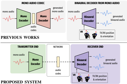
Our goal is to create a pipeline for a binaural communication system, as shown at the bottom of Fig. 1. At the transmitter end, monaural audio is first encoded by an audio encoder, and then transmitted over the network. At the receiver end, the transmitted audio code is decoded, and the binaural audio is synthesized according to transmitter and receiver positions in the virtual space. Specifically, such a system should be capable of (a) encoding transmitter audio into a low-bitrate neural code and (b) synthesizing binaural audio from these codes including environmental factors such as room reverb and noise floor, which are crucial for acoustic realism and depth perception.
Although binaural synthesis has recently experienced a breakthrough based on neural audio rendering techniques [2-4] that allow to learn binauralization and spatial audio in a datadriven way, these approaches fall short in their ability to faithfully model environmental factors such as room reverb and noise floor. The reason these models fail to model stochastic processes is their reliance on direct reconstruction losses on waveforms. Additionally, this reliance on metric losses makes the joint optimization of neural spatial renderers and neural audio codecs a difficult task. In fact, given their high sensitivity
∗ Work done while interning at Meta Reality Labs Research.
Figure 1: Illustration of previous works and the proposed system. Top left : Standard audio codec which encodes and reconstructs mono audio. Top right : binaural decoder that spatializes mono audio by conditioning on orientation and relative position between the transmitter and receiver. Bottom : proposed end-to-end binaural system that combines previous modules.
<details>
<summary>Image 1 Details</summary>
### Visual Description
## System Diagram: Mono Audio Codec and Binaural Decoder
### Overview
The image presents two system diagrams: one illustrating a "Previous Works" approach to mono audio codec, and the other depicting a "Proposed System" involving a transmitter end, network, and receiver end for binaural audio decoding from mono audio.
### Components/Axes
**Previous Works (Top)**
* **Title:** MONO AUDIO CODEC (left), BINAURAL DECODER FROM MONO AUDIO (right)
* **Left Diagram:**
* **Input:** "mono audio" (red waveform)
* **Component 1:** "Mono Encoder" (green trapezoid)
* **Intermediate:** "audio codes" (yellow rectangle)
* **Component 2:** "Mono Decoder" (red trapezoid)
* **Output:** "generated mono audio" (red waveform)
* **Right Diagram:**
* **Input:** "mono audio" (red waveform)
* **Component:** "Binaural Decoder" (purple trapezoid)
* **Output:** "generated binaural audio" (two blue waveforms)
* **Additional Inputs:** "VR" (Virtual Reality headset icon), "TX/RX position & orientation" (text near VR icon)
**Proposed System (Bottom)**
* **Title:** PROPOSED SYSTEM
* **Left Section (TRANSMITTER END):**
* **Input:** "mono audio" (red waveform)
* **Component:** "Mono Encoder" (green trapezoid)
* **Middle Section (NETWORK):**
* **Component:** "audio codes" (yellow rectangle, dashed lines connecting to adjacent sections)
* **Right Section (RECEIVER END):**
* **Component:** "Binaural Decoder" (purple trapezoid)
* **Output:** "generated binaural audio" (two blue waveforms)
* **Additional Inputs:** "VR" (Virtual Reality headset icon), "TX/RX position & orientation" (text near VR icon)
### Detailed Analysis
**Previous Works - Mono Audio Codec:**
1. **Input Audio:** A red waveform labeled "mono audio" enters the "Mono Encoder."
2. **Mono Encoder:** The green "Mono Encoder" processes the audio.
3. **Audio Codes:** The encoded audio is represented as a yellow rectangle labeled "audio codes."
4. **Mono Decoder:** The "Mono Decoder" (red) receives the audio codes.
5. **Output Audio:** A red waveform labeled "generated mono audio" exits the "Mono Decoder."
**Previous Works - Binaural Decoder from Mono Audio:**
1. **Input Audio:** A red waveform labeled "mono audio" enters the "Binaural Decoder."
2. **Binaural Decoder:** The purple "Binaural Decoder" processes the audio.
3. **Output Audio:** Two blue waveforms labeled "generated binaural audio" exit the "Binaural Decoder."
4. **VR Input:** A VR headset icon and the text "TX/RX position & orientation" indicate that the decoder uses VR-related data.
**Proposed System:**
1. **Transmitter End:**
* A red waveform labeled "mono audio" enters the "Mono Encoder" (green).
2. **Network:**
* The encoded audio is represented as a yellow rectangle labeled "audio codes." Dashed lines connect this to the "Mono Encoder" and "Binaural Decoder."
3. **Receiver End:**
* The "Binaural Decoder" (purple) receives the audio codes.
* Two blue waveforms labeled "generated binaural audio" exit the "Binaural Decoder."
* A VR headset icon and the text "TX/RX position & orientation" indicate that the decoder uses VR-related data.
### Key Observations
* The "Previous Works" section shows two separate systems: a mono audio codec and a binaural decoder.
* The "Proposed System" integrates the mono audio encoding and binaural decoding into a single system with a network component.
* Both binaural decoding systems utilize VR-related data ("VR" and "TX/RX position & orientation").
* The "Proposed System" separates the encoding and decoding processes into "Transmitter End" and "Receiver End" sections, connected by a "Network."
### Interpretation
The diagrams illustrate the evolution from separate mono audio processing and binaural decoding systems to a unified system designed for network transmission and VR integration. The "Proposed System" suggests a more complex and potentially more efficient approach to generating binaural audio from mono audio, particularly in VR applications. The separation of transmitter and receiver ends implies a system designed for remote or distributed audio processing.
</details>
to phase shifts that do not necessarily correlate with perceptual quality, metric losses are known to perform badly in pure generative tasks, including speech synthesis from compressed representations. Yet, efficient compression and encoding are required in a practical setting like an AR/VR communication system.
In this work, we demonstrate that these shortcomings of existing binauralization systems can be overcome with adversarial learning which is more powerful at matching the generator distribution with the real data distribution. Simultaneously, this paradigm shift in training spatial audio systems naturally allows their fusion with neural audio codecs for efficient transmission over a network. We present a fully end-to-end, waveform-towaveform system based on a state-of-the-art neural codec [5] and binaural decoder [2]. The proposed model borrows the codec architecture from [5] and physics-inspired elements, such as view conditioning and time warping, from [2]. We propose loss functions and a training strategy that allows for efficient training, natural sounding outputs and accurate audio spatialization. In summary, our contributions are as follows:
- we propose a first fully end-to-end binaural speech transmission system that combines low-bitrate audio codecs with high-quality binaural synthesis;
- we show that our end-to-end trained system performs better than a baseline that cascades a monaural audio codec system (top left of Fig. 1) and a binaural decoder (top right of Fig. 1);
- we demonstrate that adversarial learning allows to faithfully reconstruct realistic audio in an acoustic scene, including stochastic noise and reverberation effects that existing approaches fail to model.
## 2. Related Work.
Audio codecs have long relied on traditional signal processing and in-domain knowledge of psychoacoustics in order to perform encoding of speech [6] or general audio signals [7, 8]. More recently, following advances in speech synthesis [9-11], data-driven neural audio codecs were developed [12-16], and Soundstream [5], a novel neural audio codec, has shown to be capable of operating on bitrates as low as 3kbps with state-ofthe-art sound reconstruction quality. None of these approaches, however, was developed with spatial audio in mind, focusing solely on reconstructing monaural signals, as illustrated at the top left of Fig. 1.
Binaural audio synthesis has traditionally relied on signal processing techniques that model the physics of human spatial hearing as a linear time-invariant system [17-20]. More recently, there has been a line of studies on neural synthesis of binaural audio that showed the advantages of the data-driven approaches [2-4,21-25]. We will refer to these models, illustrated at the top right of Fig. 1, as binaural decoders . All these approaches, however, are trained as regression models with pointwise, metric losses such as mean squared error. Consequently, they fail to model stochastic processes on the receiver side that are not observable on the mono transmitter input. Examples of these processes are noise floor and reverberant effects in the virtual receiver environment.
## 3. Proposed system
## 3.1. Model architecture
Formally, we aim to find a model f that takes as input a mono audio signal x ∈ R T , and generates the left and right binaural signals ˆ y = ( ˆ y ( l ) , ˆ y ( r ) ) (both of length T ) by conditioning on a temporal signal c of length T which contains the transmitter and receiver position and orientation. Our model, depicted in Fig. 2, is based on Soundstream [5], with a series of modifications for generating binaural signals. The input signal x is first encoded with a convolutional (conv) neural network, Enc , and then discretized with a residual vector quantizer (RVQ) to obtain the audio codes, h ∈ R T M × D , where M is the downsampling rate and D is the dimension of a single code. The decoder, Dec , which consists of a convnet and a warpnet [2], then generates the binaural signals by conditioning on the position information. The process can be formulated as follows:
<!-- formula-not-decoded -->
In order to facilitate adversarial training, a set of discriminators is trained together with the entire network in an end-to-end fashion. We describe each component in detail below, and because we mostly followed the specifications described in [5], we omit detailed hyperparameters due to space constraints.
## 3.1.1. Soundstream-based encoder
The first part of the encoder is a stack of four 1D conv blocks, with each block containing three residual units and a downsampling strided conv layer. After the input mono signal is transformed into a series of continuous vectors, they are thereafter discretized through a RVQ [5, 26] of N VQ layers, which represents each vector with a sum of codewords from a set of finite codebooks. These final vectors are denoted as the audio codes . Note that in [5], several techniques are used to improve codebook usage and bitrate scalability including k-means based initialization, codeword revival and quantization dropout, which we did not find necessary in our work. During training, the codebooks are updated with exponential moving averages, following [5,27].
## 3.1.2. Partially conditioned binaural decoder
The first part of the decoder is a reverse mirror of the encoder, with the downsampling strided conv layers replaced by upsampling transposed conv layers. Because it was orginally proposed for mono audio reconstruction, we carefully designed the decoder to capture the required fidelity of the binaural signals by conditioning on the position information c . First, a FiLMbased affine layer [28] was added to the output of each conv layer. Specifically, the position information is first processed through a three-layered MLP with ReLU activation, which is then upsampled to be used as the scale and shift parameters to perform feature-wise affine transformation. Second, due to the low dimension and low frequency nature of the position vector, we further adopt a Gaussian Fourier encoding layer [29] at the beginning of the position input to learn the implicit, high frequency correlation between the position vector and the binaural audio. Moreover, we empirically discovered that it is sufficient to condition only the last few decoder blocks with position information to get high-quality binaural signals. This is because interaural differences are typically determined within a short temporal window ( ≤ 100 samples), and the position information is only needed to accurately shift and scale the binaural signals by such a small amount. Since the temporal resolution of the audio codes (determined by the encoder downsampling rate) is greater than this difference, introducing the conditioning at the start of the decoder is ineffective.
Additionally, we added a neural time warping layer proposed in [2] at the end of the decoder to model the temporal shifts from mono to binaural signals caused by sound propagation delays. The layer is a fully differentiable implementation of the monotonous dynamic time warping algorithm.
## 3.1.3. Multi-scale and single-scale discriminators
Following [5], we used two types of discriminators. The first type is a single-scale STFT discriminator, which operates on the STFT spectrogram. The architecture is based on a stack of conv layer-based residual units. The second type, originally proposed in [10], is a multi-scale discriminator (MSD) with three sub-discriminator operating on different temporal scales: 1/2/4 × downsampled version of the input signal. Each subdiscriminator is composed of a sequence of strided and grouped convolutional layers. In addition, we adopted the projection discriminator proposed in [30] to inform the multi-scale discriminator to make use of the conditional information when approximating the underlying probabilistic model given in Eq. 1. We empirically found that this significantly improves the quality of spatialization.
## 3.2. Loss function
Let the target binaural signals be y = ( y ( l ) , y ( r ) ) . Given the importance of interaural time and level differences for human auditory perception [31], we optimize the difference between the left and right predicted signal against the target signal,
<!-- formula-not-decoded -->
We additionally use a phase loss L pha that directly optimizes the phase in angular space, which has been proven crucial for accurate phase modeling in [2].
Figure 2: Model architecture. Top left : Soundstream-based encoder, consists of a stack of conv layer-based encoder blocks and a residual vector quantizer. Bottom left : Partially conditioned binaural decoder, consists of a stack of partially FiLMed decoder blocks and a WarpNet. Top right : Multi-scale projection discriminator. Bottom right : STFT discriminator.
<details>
<summary>Image 2 Details</summary>

### Visual Description
## Neural Audio Processing Diagram
### Overview
The image presents a block diagram of a neural audio processing system. It includes an encoder, a decoder, and two discriminators. The encoder converts mono audio into audio codes, which are then used by the decoder to generate binaural audio. The discriminators evaluate the generated audio.
### Components/Axes
**Encoder Section (Top-Left):**
* **Title:** Soundstream based encoder
* **Input:** mono audio (represented by a waveform)
* **Blocks:**
* Conv (Convolutional layer)
* Encoder block x4 (containing Residual unit x3)
* Strided Conv (Strided Convolutional layer)
* Residual vector quantizer (containing 1st VQ, 2nd VQ, ..., Nth VQ)
* **Output:** audio codes (represented by a vertical bar)
**Decoder Section (Bottom-Left):**
* **Title:** Partially conditioned binaural decoder
* **Input:** audio codes (represented by a vertical bar)
* **Conditioning Input:** TX/RX position & orientation (with VR headset icon)
* **Blocks:**
* Conv (Convolutional layer)
* Decoder block x2 (containing Residual unit x3)
* Transposed Conv-FiLM (Transposed Convolutional layer with FiLM conditioning)
* FiLMed decoder block x2 (containing FiLMed residual unit x3)
* Conv-FiLM (Convolutional layer with FiLM conditioning)
* WarpNet
* **Output:** generated binaural audio (represented by a waveform)
**Multi-Scale Discriminator (Top-Right):**
* **Title:** Multi scale discriminator
* **Input:** binaural audio (represented by a waveform)
* **Blocks:**
* 2x avgpool (Average pooling layer, repeated twice)
* Sub discriminator (repeated three times)
* **Conditioning Input:** TX/RX position & orientation (with VR headset icon)
* **Output:** logits (from each sub-discriminator)
**STFT Discriminator (Bottom-Right):**
* **Title:** STFT discriminator
* **Input:** binaural audio (represented by a waveform)
* **Blocks:**
* STFT layer (Short-Time Fourier Transform layer)
* Residual unit x6
* Conv (Convolutional layer)
* **Output:** logits
### Detailed Analysis or Content Details
**Encoder:**
1. Mono audio enters the encoder.
2. The audio passes through a convolutional layer (Conv).
3. The audio then goes through four encoder blocks (Encoder block x4), each containing three residual units (Residual unit x3).
4. A strided convolutional layer (Strided Conv) follows.
5. The audio is then processed by a residual vector quantizer (Residual vector quantizer), which contains multiple vector quantization stages (1st VQ, 2nd VQ, ..., Nth VQ).
6. The output of the encoder is audio codes.
**Decoder:**
1. Audio codes enter the decoder.
2. The audio codes pass through a convolutional layer (Conv).
3. The audio codes then go through two decoder blocks (Decoder block x2), each containing three residual units (Residual unit x3).
4. The audio codes are processed by a transposed convolutional layer with FiLM conditioning (Transposed Conv-FiLM).
5. The audio codes then go through two FiLMed decoder blocks (FiLMed decoder block x2), each containing three FiLMed residual units (FiLMed residual unit x3).
6. The audio codes are processed by a convolutional layer with FiLM conditioning (Conv-FiLM).
7. The audio codes are then processed by WarpNet.
8. The output of the decoder is generated binaural audio.
**Multi-Scale Discriminator:**
1. Binaural audio enters the multi-scale discriminator.
2. The audio passes through two average pooling layers (2x avgpool).
3. The audio is then processed by three sub-discriminators (Sub discriminator).
4. The output of each sub-discriminator is logits.
**STFT Discriminator:**
1. Binaural audio enters the STFT discriminator.
2. The audio passes through an STFT layer (STFT layer).
3. The audio is then processed by six residual units (Residual unit x6).
4. The audio is then processed by a convolutional layer (Conv).
5. The output of the discriminator is logits.
### Key Observations
* The system uses a combination of convolutional layers, residual units, and vector quantization to encode and decode audio.
* The decoder is conditioned on the position and orientation of the listener.
* The system uses two discriminators to evaluate the generated audio: a multi-scale discriminator and an STFT discriminator.
### Interpretation
The diagram illustrates a neural audio processing system designed for generating binaural audio from mono audio, potentially for virtual reality (VR) applications. The encoder compresses the mono audio into a set of audio codes, while the decoder reconstructs binaural audio from these codes, taking into account the listener's position and orientation. The use of FiLM conditioning in the decoder suggests that the position and orientation information is used to modulate the audio features. The multi-scale and STFT discriminators likely serve to improve the quality and realism of the generated binaural audio by penalizing artifacts and inconsistencies. The system appears to be designed to create a realistic and immersive audio experience for VR users.
</details>
We also adopted a mix of losses used in [5]. The first loss is a hinge adversarial loss, where the respective losses for the generator (the model f in Eq. 1) and the discriminator D 1 are defined as:
<!-- formula-not-decoded -->
<!-- formula-not-decoded -->
Second, the feature matching loss [10, 11] is introduced as an implicit similarity metric defined as the differences of the intermediate features from the discriminator between a ground truth and a generated sample:
<!-- formula-not-decoded -->
where L denotes the total number of layers in D and D i denotes the features from the i -th layer. Finally, the mel spectrogram loss is applied, as in [11]:
<!-- formula-not-decoded -->
where φ denotes the transform from audio to mel spectrogram.
The overall generator loss is a weighted sum of the different loss components:
<!-- formula-not-decoded -->
Our initial experiments with weights suggested in [5] ( λ fm = 100 , λ mel = 1 ) yielded poor results. Instead, we discovered that it is critical to give the mel spectrogram loss a higher weight. The final weight combination we used is: λ diff = λ adv = 1 , λ pha = 0 . 01 , λ fm = 2 , λ mel = 45 .
## 3.3. Mono pretraining
From Eq. 1, the Dec is responsible for (1) upsampling h to match the temporal resolution of x , and (2) spatialization using information from c . If the model is trained from scratch, the Dec struggles to achieve both tasks concurrently. As a result, we propose a pretraining strategy, which we found to be
1 For simplicity we assume that D outputs the average logits of all sub-discriminators in this section.
important for fast convergence and high-quality output. In the pretraining step the model is trained to generate two copies of the monaural input signals. The primary objective is to train the decoder to upsample while ignoring the condition information via a constant zero vector. Following that, the fine-tuning step is performed using the acutal binaural signals and position condition information. Once the model has been initialised to perform well at upsampling, it can be trained to spatialize and is expected to retain the ability to upsample.
## 4. Experiments
## 4.1. Experimental settings
Datasets. We re-recorded the VCTK corpus [32] using a binaural microphone setup comprised of three 3Dio Omni Pro rigs, which were placed at the center of a non-anechoic room. Speech signals were played back on a loudspeaker, which was carried by a person walking randomly around the room to cover various areas. The 3D position and orientation of the loudspeaker as well as the static 3DIO rigs were tracked using Motive Optitrack system. We recorded 42 hours of binaural audio data, covering a distance of 4.6 m horizontally and 2.4 m vertically. The audio was sampled at 48kHz and the tracking data was recorded at 240 frames per second. For mono-pretraining, we used the original monaural version of VCTK.
Competing systems. We first consider the state-of-the-art binaural decoder only system [2]. It is trained on the same binaural speech dataset. We then consider a baseline system, where we directly cascade the Soundstream [5] and the binaural decoder [2] models trained separately on VCTK and the binaural speech datasets, respectively.
Objective metrics. The 2 distance of the predicted and ground truth audio is calculated in the waveform and mel spectrogram domains. To assess the spatialization accuracy, we report the deep perceptual spatial-audio localization metric (DPLM) [33]. Subjective evaluation protocol. This evaluation is divided into two parts. In the first part, participants were presented the result of our system and a competing system (either the decoder only or the baseline system) and were asked to determine which of them is closer to the ground truth. The second part focuses on spatialization. The reference and synthetic samples are played alternating, switching between the one and the other every few
Table 1: Objective evaluation results on the competing systems and variations of the proposed systems.
| System | Wave- 2 ↓ | Mel spec- 2 ↓ | DPLM ↓ |
|-----------------|----------------------------|--------------------------------|----------|
| Decoder only | 0.228 | 1.22 | 0.108 |
| Baseline | 0.75 | 1.173 | 0.105 |
| Proposed system | 0.807 | 0.631 | 0.106 |
<details>
<summary>Image 3 Details</summary>
### Visual Description
## Stacked Bar Chart: Comparison of Approaches
### Overview
The image presents a stacked bar chart comparing the performance of "our approach" against two different baselines: "baseline" and "decoder only". The chart shows the percentage breakdown of outcomes, categorized as "our approach", "baseline" or "decoder only", and "both are bad". There are two stacked bars, one for each baseline comparison.
### Components/Axes
* **Chart Type:** Stacked Bar Chart
* **Categories:** Two comparisons are shown as two stacked bars.
* **Legend (Top):**
* Green: "our approach"
* Red: "baseline"
* Gray (with dots): "both are bad"
* **Legend (Bottom):**
* Green: "our approach"
* Red: "decoder only"
* Gray (with dots): "both are bad"
* **Values:** Percentages are displayed within each segment of the stacked bars.
### Detailed Analysis
**Top Bar (Comparison with "baseline"):**
* **"our approach" (Green):** 82.0%
* **"both are bad" (Gray):** 14.9%
* **"baseline" (Red):** 3.1%
**Bottom Bar (Comparison with "decoder only"):**
* **"our approach" (Green):** 79.4%
* **"both are bad" (Gray):** 3.4%
* **"decoder only" (Red):** 17.2%
### Key Observations
* "Our approach" consistently accounts for the largest percentage in both comparisons (82.0% and 79.4%).
* The "decoder only" baseline results in a significantly higher percentage (17.2%) compared to the "baseline" (3.1%).
* The "both are bad" category is relatively small in both comparisons (14.9% and 3.4%).
### Interpretation
The data suggests that "our approach" outperforms both the "baseline" and "decoder only" methods. The significant difference between the "baseline" and "decoder only" percentages indicates that the "decoder only" method is less effective than the "baseline" method. The relatively low percentages for "both are bad" suggest that "our approach" is generally successful, even when compared to the other methods. The stacked bar chart effectively visualizes the relative performance of "our approach" against the two baselines, highlighting its superiority.
</details>
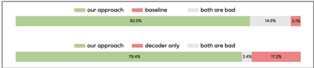
(a) Evaluation 1: participants were asked if our system or the baseline (top)/decoder only (bottom) system are closer to the ground truth.
<details>
<summary>Image 4 Details</summary>
### Visual Description
## Stacked Bar Chart: Comparison of Approaches
### Overview
The image presents a stacked bar chart comparing the performance of "our approach" against two baselines: "baseline" and "decoder only". The chart displays the percentage breakdown of each approach, indicating the proportion of cases where "our approach" is better, worse, or shows "no difference".
### Components/Axes
* **Chart Type:** Stacked Bar Chart
* **Categories:** Two categories are compared:
* Comparison 1: "our approach" vs. "baseline"
* Comparison 2: "our approach" vs. "decoder only"
* **Legend:** Located at the top of the chart, indicating the color-coding for each approach:
* Green: "our approach"
* Red: "baseline" or "decoder only"
* Light Gray with diagonal lines: "no difference"
* **Values:** Percentages are displayed within each segment of the stacked bar.
### Detailed Analysis
**Comparison 1: "our approach" vs. "baseline"**
* "our approach" (Green): 30.3%
* "no difference" (Light Gray): 60.7%
* "baseline" (Red): 9.0%
**Comparison 2: "our approach" vs. "decoder only"**
* "our approach" (Green): 17.6%
* "no difference" (Light Gray): 58.0%
* "decoder only" (Red): 17.6%
### Key Observations
* In both comparisons, "no difference" is the largest segment, indicating that in the majority of cases, "our approach" performs similarly to the baselines.
* "our approach" performs better than the "baseline" in 30.3% of cases, while the "baseline" performs better in only 9.0% of cases.
* When compared to "decoder only", "our approach" and "decoder only" perform better in the same percentage of cases (17.6%).
### Interpretation
The stacked bar chart provides a direct comparison of "our approach" against two different baselines. The data suggests that "our approach" shows a significant improvement over the "baseline" but performs similarly to the "decoder only" approach. The large "no difference" segment in both comparisons indicates that "our approach" does not consistently outperform the baselines, but it also doesn't consistently underperform. The chart highlights the need for further investigation to understand the specific scenarios where "our approach" excels or falls short compared to the baselines.
</details>
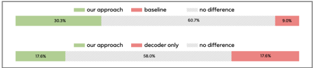
(b) Evaluation 2: participants were asked if our system or the baseline (top)/decoder only (bottom) system are more accurately spatialized.
Figure 3: Subjective evaluation results.
seconds, so the listeners can observe the change in the sound source position when the switch happens. Participants are asked which of the synthetic samples has source position closer to the reference. Participants annotated more than 350 test examples.
## 4.2. Empirical Evaluation
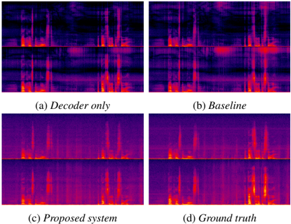
Objective Evaluation. The objective evaluation results are shown in Tab. 1. Unsurprisingly, being optimized in the waveform domain, the decoder only model outperforms others on wave 2 metric. However, the 2 -loss is not a good indicator of signal quality and can result in highly distorted signals even if the loss itself is low. The proposed system is superior in terms of mel spec 2 . We note that the mel spectrogram loss is more indicative of signal quality than the waveform 2 . In fact, spectrogram visualizations in Fig. 4 show that the proposed system matches the ground truth much better than both baseline and decoder only models. Finally, the DPLM scores shows that the proposed approach achieves the same spatialization quality as the state-of-the art binaural decoders.
User study. The subjective evaluation results are shown in Fig. 3. The first evaluation confirms that the proposed approach generates more natural outputs that are closer to the ground truth recordings than both baseline and decoder-only models. When listening to outputs generated by the baseline and decoder-only models, we found that these models have difficulty reconstructing output that is uncorrelated or only weakly correlated to the input such as room noise floor and reverberation. As a result, these effects are masked out, whereas our approach models them accurately. The second evaluation confirm that the proposed approach achieves the same level of spatialization quality as the state-of-the art binaural decoders. The results also correlated well with DPLM scores presented in Tab. 1. 2
Ablation study. We conducted ablation studies to understand
2 Audio samples can be found at https://unilight. github.io/Publication-Demos/publications/ e2e-binaural-synthesis
Figure 4: Visualizations of spectrograms from the decoder only, baseline, proposed system and the ground truth.
<details>
<summary>Image 5 Details</summary>
### Visual Description
## Spectrogram Comparison: Speech Synthesis Models
### Overview
The image presents a visual comparison of spectrograms generated by different speech synthesis models, including a "Decoder only" model, a "Baseline" model, a "Proposed system," and the "Ground truth" spectrogram. Each model's output is displayed as a spectrogram, showing frequency content over time. The spectrograms are displayed in a 2x2 grid.
### Components/Axes
Each spectrogram displays frequency on the vertical axis and time on the horizontal axis, though specific scales are not provided. The color intensity represents the magnitude of the frequency components, with darker colors indicating lower magnitudes and brighter colors (towards red/yellow) indicating higher magnitudes.
The subplots are labeled as follows:
* **(a) Decoder only**: Spectrogram generated by a decoder-only model.
* **(b) Baseline**: Spectrogram generated by a baseline model.
* **(c) Proposed system**: Spectrogram generated by the proposed system.
* **(d) Ground truth**: Spectrogram representing the actual speech signal.
### Detailed Analysis
Each spectrogram is divided into two horizontal sections, presumably representing different aspects of the audio signal or different channels.
* **(a) Decoder only**: The spectrogram shows some distinct vertical bands, indicating the presence of specific frequencies over time. The intensity is generally lower compared to the other spectrograms.
* **(b) Baseline**: This spectrogram shows more intense frequency components compared to the "Decoder only" model, with some distinct vertical bands and some areas of higher intensity.
* **(c) Proposed system**: The spectrogram generated by the proposed system appears to have a higher resolution and more distinct frequency components compared to the "Decoder only" and "Baseline" models. It shows clear vertical bands and areas of high intensity.
* **(d) Ground truth**: The "Ground truth" spectrogram shows the actual speech signal, with distinct vertical bands and areas of high intensity. It serves as a reference for evaluating the performance of the other models.
### Key Observations
* The "Proposed system" spectrogram visually resembles the "Ground truth" spectrogram more closely than the "Decoder only" and "Baseline" spectrograms.
* The "Decoder only" spectrogram appears to have the lowest intensity and least defined frequency components.
* The "Baseline" spectrogram shows some improvement over the "Decoder only" spectrogram but is still less defined than the "Proposed system" and "Ground truth" spectrograms.
### Interpretation
The image suggests that the "Proposed system" is more effective at capturing the frequency characteristics of the speech signal compared to the "Decoder only" and "Baseline" models. The closer resemblance of the "Proposed system" spectrogram to the "Ground truth" spectrogram indicates that the proposed system is better at synthesizing speech that is similar to the actual speech signal. The spectrograms provide a visual representation of the performance of different speech synthesis models, allowing for a qualitative comparison of their outputs.
</details>
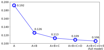
Figure 5: Distances calculated by the deep perceptual spatialaudio localization metric (DPLM) from different variations of the model. Smaller the better. A : mel spectrogram loss ( L mel ). B : adversarial-related loss ( L adv + L fm ). C : mono pretraining. D : partially-conditioned decoder. E : projection discriminator.
<details>
<summary>Image 6 Details</summary>
### Visual Description
## Line Chart: Model Performance with Feature Inclusion
### Overview
The image is a line chart illustrating the performance of a model as features are added incrementally. The x-axis represents the features included in the model (A, A+B, A+B+C, A+B+C+D, A+B+C+D+E), and the y-axis represents a performance metric, presumably an error rate or loss, ranging from 0.100 to 0.200. The line shows a decreasing trend, indicating that adding more features generally improves the model's performance.
### Components/Axes
* **X-axis:** Represents the features included in the model. The categories are:
* A
* A+B
* A+B+C
* A+B+C+D
* A+B+C+D+E (full model)
* **Y-axis:** Represents the performance metric, ranging from 0.100 to 0.200 in increments of 0.020.
* 0.100
* 0.120
* 0.140
* 0.160
* 0.180
* 0.200
* **Line:** A blue line connects the data points, showing the trend in model performance.
### Detailed Analysis
The blue line starts at a value of 0.192 when only feature A is included. As more features are added, the line slopes downward, indicating improved performance.
* **A:** 0.192
* **A+B:** 0.126
* **A+B+C:** 0.113
* **A+B+C+D:** 0.109
* **A+B+C+D+E (full model):** 0.106
### Key Observations
* The most significant performance improvement occurs when feature B is added to feature A (from 0.192 to 0.126).
* The performance improvement diminishes as more features are added beyond A+B.
* The full model (A+B+C+D+E) achieves the best performance, with a value of 0.106.
### Interpretation
The chart suggests that adding features to the model generally improves its performance, as indicated by the decreasing trend of the line. However, the marginal benefit of adding each additional feature decreases as more features are included. The most significant improvement comes from adding feature B to feature A. This could indicate that feature B is highly informative or complementary to feature A. The full model achieves the best performance, but the difference between the performance of A+B+C+D and the full model is relatively small, suggesting that features C, D, and E contribute less to the model's performance than features A and B.
</details>
the impact of various design choices in the proposed system by gradually adding components and calculating the DPLM distances of different model variations. Results are shown in Fig. 5. We see that all model components contribute to the DPLM metric, demonstrating the significance of our design choices.
Effectiveness of the adversarial loss. Note especially the importance of the adversarial loss for spatialization (A vs. A+B in Fig. 5). Due to the information bottleneck in the quantized audio codes, not all phase information is sufficiently maintained and reconstructable using a metric loss only. With the addition of adversarial loss, the model is able to generate a plausible phase, resulting in a significant improvement in spatialization quality. In addition, we found that the adversarial loss to be effective at capturing effects such as background noise and reverberation. This can be observed from the spectrograms shown in Figure 4. Because the decoder-only and baseline methods are trained without adversarial loss, the generated speech lacks background noise and reverb details, making the output binaural sound uncanny.
## 5. Conclusions
Wedescribed in detail an the end-to-end binaural speech synthesis system capable of (1) transmitting source monaural speech in the form of compressed speech codes, and (2) synthesizing accurate spatialized binaural speech by conditioning on source and receiver position/orientation information in virtual space. We tested our method on a real-world binaural dataset and found it to be objectively and subjectively superior to a cascade baseline. Finally, we conducted ablation studies to justify various design choices.
## 6. References
- [1] C. Hendrix and W. Barfield, 'The Sense of Presence within Auditory Virtual Environments,' Presence: Teleoper. Virtual Environ. , vol. 5, no. 3, p. 290-301, 1996.
- [2] A. Richard, D. Markovic, I. D. Gebru, S. Krenn, G. A. Butler, F. Torre, and Y. Sheikh, 'Neural Synthesis of Binaural Speech From Mono Audio,' in Proc. ICLR , 2021.
- [3] I. D. Gebru, D. Markovi´ c, A. Richard, S. Krenn, G. A. Butler, F. De la Torre, and Y. Sheikh, 'Implicit HRTF Modeling Using Temporal Convolutional Networks,' in Proc. ICASSP , 2021, pp. 3385-3389.
- [4] A. Richard, P. Dodds, and V. K. Ithapu, 'Deep impulse responses: Estimating and parameterizing filters with deep networks,' in IEEE International Conference on Acoustics, Speech and Signal Processing , 2022.
- [5] N. Zeghidour, A. Luebs, A. Omran, J. Skoglund, and M. Tagliasacchi, 'SoundStream: An End-to-End Neural Audio Codec,' IEEE/ACM TASLP , vol. 30, pp. 495-507, 2022.
- [6] D. O'Shaughnessy, 'Linear predictive coding,' IEEE Potentials , vol. 7, no. 1, pp. 29-32, 1988.
- [7] J. Valin, M. Corporation, K. Vos, and T. Terriberry, 'Definition of the Opus Audio Codec,' 2012.
- [8] M. Dietz, M. Multrus, V. Eksler, V. Malenovsky, E. Norvell, H. Pobloth, L. Miao, Z. Wang, L. Laaksonen, A. Vasilache, Y. Kamamoto, K. Kikuiri, S. Ragot, J. Faure, H. Ehara, V. Rajendran, V. Atti, H. Sung, E. Oh, H. Yuan, and C. Zhu, 'Overview of the EVS codec architecture,' in Proc. ICASSP , 2015, pp. 5698-5702.
- [9] A. v. d. Oord, S. Dieleman, H. Zen, K. Simonyan, O. Vinyals, A. Graves, N. Kalchbrenner, A. Senior, and K. Kavukcuoglu, 'Wavenet: A generative model for raw audio,' arXiv preprint arXiv:1609.03499 , 2016.
- [10] K. Kumar, R. Kumar, T. de Boissiere, L. Gestin, W. Teoh, J. Sotelo, A. de Br´ ebisson, Y . Bengio, and A. C. Courville, 'MelGAN: Generative Adversarial Networks for Conditional Waveform Synthesis,' in Proc. NeurIPS , vol. 32, 2019.
- [11] J. Kong, J. Kim, and J. Bae, 'HiFi-GAN: Generative Adversarial Networks for Efficient and High Fidelity Speech Synthesis,' in Proc. NeurIPS , vol. 33, 2020, pp. 17 022-17 033.
- [12] W. B. Kleijn, F. S. C. Lim, A. Luebs, J. Skoglund, F. Stimberg, Q. Wang, and T. C. Walters, 'Wavenet Based Low Rate Speech Coding,' in Proc. ICASSP , 2018, pp. 676-680.
- [13] C. Gˆ arbacea, A. v. den Oord, Y. Li, F. S. C. Lim, A. Luebs, O. Vinyals, and T. C. Walters, 'Low Bit-rate Speech Coding with VQ-VAE and a WaveNet Decoder,' in Proc. ICASSP , 2019, pp. 735-739.
- [14] K. Zhen, M. S. Lee, J. Sung, S. Beack, and M. Kim, 'Efficient And Scalable Neural Residual Waveform Coding with Collaborative Quantization,' in Proc. ICASSP , 2020.
- [15] W. B. Kleijn, A. Storus, M. Chinen, T. Denton, F. S. C. Lim, A. Luebs, J. Skoglund, and H. Yeh, 'Generative Speech Coding with Predictive Variance Regularization,' in Proc. ICASSP , 2021, pp. 6478-6482.
- [16] A. Polyak, Y. Adi, J. Copet, E. Kharitonov, K. Lakhotia, W.-N. Hsu, A. Mohamed, and E. Dupoux, 'Speech Resynthesis from Discrete Disentangled Self-Supervised Representations,' in Proc. Interspeech , 2021.
- [17] L. Savioja, J. Huopaniemi, T. Lokki, and R. V¨ a¨ an¨ anen, 'Creating Interactive Virtual Acoustic Environments,' Journal of the Audio Engineering Society , vol. 47, no. 9, pp. 675-705, 1999.
- [18] D. Zotkin, R. Duraiswami, and L. Davis, 'Rendering localized spatial audio in a virtual auditory space,' IEEE Transactions on Multimedia , vol. 6, no. 4, pp. 553-564, 2004.
- [19] K. Sunder, J. He, E. L. Tan, and W.-S. Gan, 'Natural Sound Rendering for Headphones: Integration of signal processing techniques,' IEEE Signal Processing Magazine , vol. 32, no. 2, pp. 100-113, 2015.
- [20] W. Zhang, P. Samarasinghe, H. Chen, and T. Abhayapala, 'Surround by Sound: A Review of Spatial Audio Recording and Reproduction,' Applied Sciences , vol. 7, p. 532, 05 2017.
- [21] P. Morgado, N. Nvasconcelos, T. Langlois, and O. Wang, 'SelfSupervised Generation of Spatial Audio for 360° Video,' in Proc. NeurIPS , vol. 31, 2018.
- [22] R. Gao and K. Grauman, '2.5 d Visual Sound,' in Proc. CVPR , 2019, pp. 324-333.
- [23] Y.-D. Lu, H.-Y. Lee, H.-Y. Tseng, and M.-H. Yang, 'SelfSupervised Audio Spatialization with Correspondence Classifier,' in Proc. ICIP , 2019, pp. 3347-3351.
- [24] K. Yang, B. Russell, and J. Salamon, 'Telling Left From Right: Learning Spatial Correspondence of Sight and Sound,' in Proc. CVPR , 2020.
- [25] H. Zhou, X. Xu, D. Lin, X. Wang, and Z. Liu, 'Sep-stereo: Visually guided stereophonic audio generation by associating source separation,' in Proc. ECCV , 2020.
- [26] A. van den Oord, O. Vinyals, and k. Kavukcuoglu, 'Neural Discrete Representation Learning,' in Proc. NIPS , 2017, pp. 63066315.
- [27] A. Razavi, A. Van den Oord, and O. Vinyals, 'Generating Diverse High-fidelity Images with VQ-VAE-2,' in Proc. NeurIPS , 2019.
- [28] E. Perez, F. Strub, H. De Vries, V. Dumoulin, and A. Courville, 'FiLM: Visual Reasoning with a General Conditioning Layer,' in Proc. AAAI , vol. 32, no. 1, 2018.
- [29] M. Tancik, P. Srinivasan, B. Mildenhall, S. Fridovich-Keil, N. Raghavan, U. Singhal, R. Ramamoorthi, J. Barron, and R. Ng, 'Fourier features let networks learn high frequency functions in low dimensional domains,' in Proc. NeurIPS , 2020, pp. 75377547.
- [30] T. Miyato and M. Koyama, 'cGANs with Projection Discriminator,' in Proc. ICLR , 2018.
- [31] C. Darwin and R. Hukin, 'Auditory objects of attention: the role of interaural time differences.' Journal of Experimental Psychology: Human perception and performance , vol. 25, no. 3, p. 617, 1999.
- [32] C. Veaux, J. Yamagishi, and K. MacDonald, 'CSTR VCTK Corpus: English Multi-speaker Corpus for CSTR Voice Cloning Toolkit,' 2017.
- [33] P. Manocha, A. Kumar, B. Xu, A. Menon, I. D. Gebru, V. K. Ithapu, and P. Calamia, 'DPLM: A Deep Perceptual SpatialAudio Localization Metric,' in Proc. Workshop on Applications of Signal Processing to Audio and Acoustics (WASPAA) , 2021, pp. 6-10.