# BAST: Binaural Audio Spectrogram Transformer for Binaural Sound Localization
**Authors**: Sheng Kuang, Jie Shi, Kiki van der Heijden, Siamak Mehrkanoon
> Department of Information and Computing Sciences, Utrecht University, Utrecht, The Netherlands Department of Data Science and Knowledge Engineering, Maastricht University, The Netherlands. Donders Institute for Brain Cognition and Behavior, Radboud University, Nijmegen, The Netherlands
## Abstract
Accurate sound localization in a reverberation environment is essential for human auditory perception. Recently, Convolutional Neural Networks (CNNs) have been utilized to model the binaural human auditory pathway. However, CNN shows barriers in capturing the global acoustic features. To address this issue, we propose a novel end-to-end Binaural Audio Spectrogram Transformer (BAST) model to predict the sound azimuth in both anechoic and reverberation environments. Two modes of implementation, i.e. BAST-SP and BAST-NSP corresponding to BAST model with shared and non-shared parameters respectively, are explored. Our model with subtraction interaural integration and hybrid loss achieves an angular distance of 1.29 degrees and a Mean Square Error of 1e-3 at all azimuths, significantly surpassing CNN based model. The exploratory analysis of the BAST’s performance on the left-right hemifields and anechoic and reverberation environments shows its generalization ability as well as the feasibility of binaural Transformers in sound localization. Furthermore, the analysis of the attention maps is provided to give additional insights on the interpretation of the localization process in a natural reverberant environment.
keywords: Transformer , Sound localization , Binaural integration journal: A
## 1 Introduction
Sound source localization is a fundamental ability in everyday life. Accurately and precisely localizing incoming auditory streams is required for auditory perception and social communication. In the past decades, the biological basis and neural mechanism of sound localization have been extensively explored [1, 2, 3, 4]. Normal hearing listeners extract horizontal acoustic cues by mainly relying on the interaural level differences (ILD) and interaural time differences (ITD) of the auditory input. These cues are encoded through the human auditory subcortical pathway, in which the auditory structures in the brainstem integrate and convey the binaural signals from cochleas to the auditory cortex [2, 4]. However, sound localization is frequently affected by the noise and reverberations in the complex real-word environment, which distort the spatial cues of the sound source of interest [5]. Yet, it is still not clear how the spatial position of acoustic signals in complex listening environments is extracted by the human brain.
Recently, Deep Learning (DL) [6] has been proposed to model auditory processing and has achieved great success. These approaches enable optimization of auditory models for real-life auditory environment [7, 8, 9, 10]. In the early attempts, DL methods were combined with conventional feature engineering to deal with the noise and reverberation problems [7, 11]. For instance, in [7], binaural spectral and spatial features were separately extracted, providing complementary information for a two-layer Deep Neural Network (DNN). Similarly, in [8, 12, 13], deep neural networks were used to de-noise and de-reverberate complex sound stimuli. In a CNN-based azimuth estimation approach, researchers utilized a Cascade of Asymmetric Resonators with Fast-Acting Compression to analyze sound signals and used onsite-generated correlograms to eliminate the echo interference [14]. However, most of these approaches highly depend on feature selection. To reduce this constraint, end-to-end Deep Residual Network (DRN) was recommended [15, 16]. Instead of selecting features from acoustic signal, raw spectrograms of sound was utilized in Deep Residual Network for azimuth prediction [16]. DRN was shown to be robust even in the presence of unknown noise interference at the low signal-to-noise ratio. Subsequently, [9] proposed a pure attention-based Audio Spectrogram Transformer (AST) and achieved the state-of-the-art results for audio classification on multiple datasets. Although these DL-based methods have yielded promising results, however due to a lack of similar architectures to the human binaural auditory pathway, they may not resemble the neural processing of sound localization.
To encode the neural mechanisms underlying sound localization, the performance of deep learning methods is commonly compared to the human sound localization behavior [17, 18, 19]. For instance, [19] systematically explored the performance of binaural sound clips localization of a CNN in a real-life listening environment, however, its architecture does not resemble the structure of human auditory pathway. This issue has been addressed by utilizing a hierarchical neurobiological-inspired CNN (NI-CNN) to model the binaural characteristics of human spatial hearing [17]. This unique hierarchical design, models the binaural signal integration process and is shown to have brain-like latent feature representations. However, NI-CNN [17] is not an end-to-end model as it leverages a cochlear method to generate auditory nerve representations as model input. Furthermore, considering the wide range of frequencies of sound input, the convolution operations in NI-CNN mainly extract local-scale features and therefore may exhibit limitations for extracting global features in the acoustic time-frequency spectrogram.
In this study, we build on the success and barriers of previously proposed deep neural networks at localizing sound sources to further develop an end-to-end transformer based model for human sound localization, which captures the global acoustic features from auditory spectrograms. We aimed at (i) investigating the performance of a pure Transformer-based hierarchical binaural neural network for addressing human real-life sound localization; (ii) exploring the effect of various loss functions and binaural integration methods on the localization acuity at different azimuths; (iii) visualizing the attention flow of the proposed model to demonstrate the localization process.
<details>
<summary>x1.png Details</summary>
### Visual Description
## Diagram: Transformer-Based Stereo Vision Architecture for Depth Estimation
### Overview
The diagram illustrates a transformer-based architecture for stereo vision depth estimation, divided into three components: (a) the overall system workflow, (b) detailed transformer encoder structure, and (c) interaural integration methods. The system processes stereo image pairs to estimate depth maps through patch embeddings, transformer encoding, and fusion of left/right view information.
### Components/Axes
#### Part (a): System Workflow
1. **Input**: Stereo image pair (Left/Right views) with overlapping patches.
2. **Preprocessing**:
- Linear Projection → Patch Embeddings
- Position Embeddings added to patch embeddings
3. **Encoding**:
- Separate Transformer Encoders (L for Left, R for Right)
- Interaural Integration combines L and R outputs
4. **Postprocessing**:
- Transformer Encoder-C (combined encoder)
- Average over patches → Linear Layer (outputs (x, y) ∈ ℝ²)
#### Part (b): Transformer Encoder Details
1. **Core Components**:
- Patch Embeddings (3×3 grid)
- Layer Normalization
- Multi-Head Attention
- MLP (Multi-Layer Perceptron)
2. **Flow**:
- Input → Patch Embeddings → Layer Norm → Multi-Head Attention → Layer Norm → MLP → Output Sequence
#### Part (c): Interaural Integration Methods
1. **Method 1: Concatenation**
- Input: Left (D×N_H×N_T) and Right (D×N_H×N_T)
- Output: 2D×N_H×N_T
2. **Method 2: Addition**
- Input: Left (D×N_H×N_T) + Right (D×N_H×N_T)
- Output: D×N_H×N_T
3. **Method 3: Subtraction**
- Input: Left (D×N_H×N_T) - Right (D×N_H×N_T)
- Output: D×N_H×N_T
### Detailed Analysis
- **Patch Generation**: Overlapping patches (N_P×N_P) extracted from both views.
- **Embeddings**: Patch and position embeddings encode spatial information.
- **Transformer Encoders**:
- Encoder-L/R process left/right views independently.
- Encoder-C integrates features from both views.
- **Integration Methods**:
- Concatenation preserves full spatial-temporal information.
- Addition/Subtraction create difference maps for disparity estimation.
### Key Observations
1. **Stereo Fusion**: The architecture explicitly models left/right view relationships through dedicated integration methods.
2. **Transformer Depth**: Uses standard transformer components (attention, MLP) adapted for vision tasks.
3. **Output Structure**: Final linear layer maps to 2D coordinates (x, y), likely representing depth estimation.
### Interpretation
This architecture demonstrates a vision transformer (ViT) approach to stereo depth estimation, leveraging:
1. **Multi-View Processing**: Separate encoders for left/right views maintain view-specific features.
2. **Feature Fusion**: Three integration methods (concat/add/subtract) enable flexible combination of view information.
3. **Depth Representation**: The 2D output suggests a coordinate-based depth map rather than per-pixel disparity.
The use of transformer encoders allows the model to capture long-range spatial dependencies crucial for accurate depth estimation, while the interaural integration methods provide multiple pathways to combine stereo information. The architecture's design suggests a focus on both feature-level fusion (addition/subtraction) and holistic view combination (concatenation).
</details>
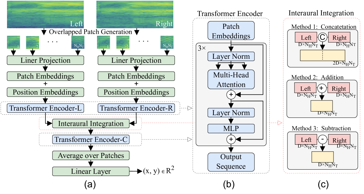
Figure 1: Architecture of the proposed Binaural Audio Spectrogram Transformer (BAST). (a) The architecture of the proposed model. (Here there are $N_{H}N_{T}$ number of patches). (b) The architecture of a single Transformer encoder. (c) Three examined interaural integration methods: concatenation, addition and subtraction.
## 2 Related Works
Binaural auditory models utilize head-related transfer functions to apply characteristics of human binaural hearing to monaural sound clips in order to simulate human spatial hearing. Conventional methods for sound source localization (SSL) have been based on microphone arrays and can be categorized into controllable beamforming, high-resolution spectrogram estimation, and time difference of sound techniques [20]. These conventional signal processing techniques are often used as baselines or input feature extraction for DL-based SSL methods. STEF (Short-Time Fourier Transform) [21] approach is used to convert the time-domain signals from each microphone into the time-frequency domain. The STFT provides a representation of the signal in both time and frequency, allowing for the analysis of how the frequency content of the signal evolves. Mixture Model (GMM), commonly used in machine learning-based studies, calculates the probability distribution of the source location in reverberant environments [22]. Gaussian mixture regression (GMR) was extended later to localize multi-source sounds [23]. Subsequently, model-based methods have been encouraged to extract ILD and ITD cues for DNN training [7]. Compressive sensing and sparse recovery techniques are extensively applied in acoustics. Sparse Bayesian learning (SBL) integrates the Bayesian framework with the concepts of sparse representations and compressive sensing. SBL has been used for SSL [24, 25, 26, 27]. However, the performance of these hybrid techniques remains unstable since the feature extraction routine varies across different datasets.
Advancements in deep learning have led to the development of convolutional neural network (CNN) based methods for sound source localization. The CNN designed by [28] uses the multichannel STFT phase spectrograms to predict multi-speakers’ azimuth in reverberant environments. The model consists of three convolutional layers with 64 filters of size ${2}\times{1}$ to consider neighboring frequency bands and microphones. Some deeper CNN architectures [29, 30, 31, 32] are applied to estimate both the azimuth and elevation. Several three-dimensional convolutions networks [33, 34] report that networks for time, frequency, and channel can achieve better accuracy than 2D convolutions. Focusing on binaural audio-visual localization, Binaural Audio-Visual Network (BAVNet) [35], for pixel-level sound source localization using binaural recordings and videos, which significantly improves performance over traditional monaural audio methods, especially when visual information quality is limited. As a data-driven DL method, NI-CNN can learn latent features for azimuth prediction from human auditory nerve representations [17]. These studies highlight the importance of advanced neural network architectures and feature extraction methods for enhancing the accuracy and resolution of sound source localization systems.
Transformer was initially proposed in natural language processing to handle long-range dependencies [36, 37]. Recently, the Transformer was successfully applied in computer vision by casting images into patch embedding sequences [38, 39]. Many hybrid models combined the Transformer with a CNN or Recurrent Neural Network (RNN) in audio processing, and some studies even directly embedded attention blocks into CNN or RNN to capture global features in a parameter-efficient way [40, 41, 42, 43]. Transformer-based models in sound source localization have gained significant attention in recent years. [44] uses a transformer encoder with residual connections and evaluates various configurations to manage multiple sound events. PILOT [45] is a transformer-based framework for sound event localization, capturing temporal dependencies through self-attention mechanisms and representing estimated positions as multivariate Gaussian variables to include uncertainty. Transformer-based models in sound event tasks have gained significant attention in recent years. The Audio Pyramid Transformer (APT) [46] with attention mechanism for weakly supervised sound event detection and audio classification, highlighting the application of transformer-based models in audio tasks. Multi-head self-attention, the parallel use of several attention layers in transformers, has also been used in SSL. Employing the first-order Ambisonic signals, Subsequently, the authors in [9] introduced AST which uses a Transformer model and variable-length monaural spectrograms to perform sound classification tasks. AST uses the overlapped-patch embedding generation policy to convert the intra-patch local features to inter-patch attention weights as a convolution-free, pure attention-based model. AST has achieved state-of-the-art [47, 48] results on multiple datasets for audio classification tasks.
The Vision Transformer (ViT) [38] represents a significant shift in the architecture of deep learning models for computer vision tasks. ViT divides an image into a sequence of fixed-size patches, linearly embedding them, and then processes them as tokens in a standard Transformer model. This method leverages the self-attention mechanism to capture long-range dependencies and contextual information across the image. The Audio Vision Transformer (AViT) is a model architecture that extends the concepts of Vision Transformers (ViTs) into the domain of audio processing. The audio-spectrogram vision transformer (AS-ViT) [49] use vision transformer models to analyze audio-spectrogram images for identifying abnormal respiratory sounds. The potential of ViT in audio-visual tasks such as sound source localization has been recognized [50]. Additionally, HTS-AT [51], a hierarchical token-semantic audio transformer, was designed to reduce the model size and training time, addressing the limitations of existing audio transformers. Binaural sound localization in noisy environments has been investigated using Frequency-Based Audio Vision Transformer (FAViT) [52]. FAViT uses selective attention mechanisms inspired by the Duplex Theory, outperforming recent CNNs and standard audio ViT models in localizing noise speech. ViT-based localization has also been explored for through-ice or underwater acoustic tracking [53].
## 3 Method
### 3.1 Model architecture
The proposed Binaural Audio Spectrogram Transformer (BAST), is illustrated in Fig. 1. Similar to NI-CNN [17], a dual-input hierarchical architecture is utilized to simulate the human subcortical auditory pathway. As opposed to NI-CNN which uses convolution layers, here three Transformer Encoders (i.e., left, right and center), hereafter called TE-L, TE-R and TE-C are utilized to construct a pure attention-based model. In particular, the pre-processed left and right sound waves are converted to left and right spectrograms denoted by $x^{L}\in\mathbb{R}^{H\times T}$ and $x^{R}\in\mathbb{R}^{H\times T}$ . Here, $H$ indicates the frequency band and $T$ indicates the number of Tukey windows ( with shape parameter: 0.25).
In what follows, the TE-L path to process the input data is explained. The other path, i.e TE-R, follows the same process. At the beginning of patch embedding layer, the left spectrogram $x^{L}\in\mathbb{R}^{H\times T}$ is first decomposed into an overlapped-patch sequence $x_{patch}^{L}\in\mathbb{R}^{P^{2}\times(N_{H}N_{T})}$ , where $P$ is the patch size, $N_{H}$ and $N_{T}$ are the number of patches in height and width respectively obtained as follows,
$$
N_{H}=\left\lceil\frac{H-P+S}{S}\right\rceil,N_{T}=\left\lceil\frac{T-P+S}{S}
\right\rceil. \tag{1}
$$
In case $H-P$ and $T-P$ are not divisible by the stride $S$ between patches, the spectrogram is zero-padded on the top and right respectively. A trainable linear projection is added to flatten each patch to a $D$ dimensional latent representation, hereafter called patch embeddings [38]. Since our model outputs the sound location coordinates, the classification token in the Transformer encoder is removed. A fixed absolute position embedding [38] is added to the patch embeddings to capture the position information of the spectrogram in the Transformer. Here, the learnable position embedding is not used as it did not significantly change model performance compared to absolute position embedding [9]. The output of the left position embedding layer $z_{in}^{L}\in\mathbb{R}^{D\times(N_{H}N_{T})}$ is then fed to the Transformer encoder TE-L.
We use the identical Transformer encoder design in [38, 9], consisting of $K$ stacked Multi-head Self-Attention (MSA) and Multi-Layer Perceptron (MLP) blocks. The BAST model performance is compared when using shared and non-shared parameters across the left and right Transformer encoders. Hereafter, BAST-SP refers to BAST model whose left and right Transformer encoders share parameters whereas in BAST-NSP the parameters of the left and right Transformer encoders are not shared. The output of left and right Transformer encoder, i.e., $z_{out}^{L}$ and $z_{out}^{R}$ , represents neural signals underlying the initial auditory processing stage along the left and right auditory pathway respectively. Subsequently, these binaural feature maps are integrated to simulate the function of the human olivary nucleus. Similar to NI-CNN, here three integration methods, i.e. addition, subtraction and concatenation, are investigated. Specifically, addition is the summation of feature maps of both sides; subtraction represents left feature map subtracted from the right feature map; concatenation is implemented by concatenating $z_{out}^{L}$ and $z_{out}^{R}$ along the the first dimension to produce $z_{in}^{C}\in\mathbb{R}^{2D\times(N_{H}N_{T})}$ . TE-C receives the integrated feature map $z_{in}^{C}$ and output sequence $z_{out}^{C}$ . Next, an average operation of the patch dimension and a linear transformer layer is applied to finally produce the sound location coordinates $(x,y)$ . The last linear layer does not have any activation function, therefore the estimated coordinates can be any point on the 2D plane.
### 3.2 Loss Function
Three loss functions, i.e., Angular Distance (AD) loss [54], Mean Square Error (MSE) loss, as well as hybrid loss with a convex combination of AD and MSE, are explored in training the proposed model. Let $C_{i}=(x_{i},y_{i})$ and $\hat{C}_{i}=(\hat{x}_{i},\hat{y}_{i})$ denote the ground truth and predication coordinates for the i- $th$ sample. MSE loss measures the squared difference of Euclidean distance between the prediction and the ground truth as follows:
$$
\textrm{MSE}=\frac{1}{N}\sum_{i}^{N}\|C_{i}-\hat{C}_{i}\|_{2}^{2}, \tag{2}
$$
where $(\hat{x_{i}},\hat{y_{i}})$ is the predicted coordinates, $(x_{i},y_{i})$ is the true sound location and $N$ is the batch size. Note that MSE loss is able to penalize the large Euclidean distance error but is insensitive to the angular distance, which means that the azimuth may differ with the same MSE. In contrast to MSE, AD loss merely measures the angular distance while ignoring the Euclidean distance:
$$
\textrm{AD}=\frac{1}{\pi N}\sum^{N}_{i}\arccos{(\frac{C_{i}\hat{C}_{i}^{T}}{\|
C_{i}\|_{2}\|\hat{C}_{i}\|_{2}})}, \tag{3}
$$
where $C_{i},\hat{C}_{i}\neq 0$ .
Table 1: The performance of BAST-NSP and BAST-SP compared to NI-CNN and NI-CNN ∗ when different loss and binaural integration methods are used. The best performed model in AD and MSE are in bold. The ↓ indicates the lower the value of the metric, the better the model performance.
| Model | Loss | Angular Distance(AD) ↓ | Mean Squared Error (MSE) ↓ | | | | | | |
| --- | --- | --- | --- | --- | --- | --- | --- | --- | --- |
| SS | Concatenation | Addition | Subtraction | SS | Concatenation | Addition | Subtraction | | |
| CNN [28] ∗ | MSE | 3.90° | — | — | — | 0.010 | — | — | — |
| AD | 42.69° | — | — | — | — | — | — | — | |
| Hybrid | 3.09° | — | — | — | 0.011 | — | — | — | |
| FAVit [52] ∗ | MSE | 6.26° | — | — | — | 0.022 | — | — | — |
| AD | 17.37° | — | — | — | — | — | — | — | |
| Hybrid | 3.73° | — | — | — | 0.015 | — | — | — | |
| NI-CNN [17] | MSE | — | 4.80° | 4.80° | 5.30° | — | 0.011 | 0.013 | 0.014 |
| AD | — | 3.70° | 3.90° | 5.20° | — | — | — | — | |
| NI-CNN [17] ∗ | MSE | — | 8.92° | 3.51° | 3.67° | — | 0.077 | 0.032 | 0.038 |
| AD | — | 7.85° | 1.97° | 1.85° | — | — | — | — | |
| Hybrid | — | 8.35° | 3.53° | 3.19° | — | 0.074 | 0.033 | 0.031 | |
| BAST-NSP | MSE | — | 2.78° | 2.48° | 2.42° | — | 0.003 | 0.002 | 0.002 |
| AD | — | 2.39° | 1.30° | 1.63° | — | — | — | — | |
| Hybrid | — | 2.76° | 1.83° | 1.29° | — | 0.004 | 0.002 | 0.001 | |
| BAST-SP | MSE | — | 2.02° | 4.97° | 1.94° | — | 0.002 | 0.018 | 0.002 |
| AD | — | 2.66° | 13.87° | 1.43° | — | — | — | — | |
| Hybrid | — | 1.98° | 5.72° | 2.03° | — | 0.003 | 0.026 | 0.002 | |
Table 2: The number of layers in each Transform encoder as well as the total number of trainable parameters of the proposed models. Tuple ( $\cdot$ , $\cdot$ , $\cdot$ ) indicates the number of layers in the left, right and center Transformer encoder respectively.
| Model | Interaural Integration | Transformer Layers | Trainable Parameters |
| --- | --- | --- | --- |
| BAST-NSP | Concatenation | (3, 3, 3) | ~76M |
| Addition/ Subtraction | (3, 3, 3) | ~57M | |
| BAST-SP | Concatenation | (3, 3, 3) | ~57M |
| Addition/ Subtraction | (3, 3, 3) | ~38M | |
## 4 Experiments
### 4.1 Dataset
We use the binaural audio data in [17], which consists of a training dataset and an independent testing dataset. In the training dataset, 4600 real-life sound waves (duration:500 ms, sampling rate: 16000) are placed in 36 azimuth positions, respectively, with $10\degree$ azimuth resolution, $0\degree$ elevation, and 1-meter distance from the center point. In addition, sound waves are spatialized with two acoustic environments, i.e. an anechoic environment (AE) without reverberation and a 10m $\times$ 14m lecture hall with reverberation (RV). In particular, here the training and test sets contain data from both AE and RV environments. In total, the training dataset has 331200 binaural learning samples. Similarly, the independent testing dataset contains 400 new sound waves processed with the same method as described above, producing 28800 testing samples.
### 4.2 Baseline methods
In this study, we establish a comprehensive framework for evaluating the performance of our proposed model by comparing it against four baseline models widely utilized in the field. Four baseline models were employed in this work: two-stream CNN-based models NI-CNN ∗ [17] and NI-CNN [17], one-stream CNN model [28], and ViT-based FAViT [52]. NI-CNN and NI-CNN ∗ models use cochleogram and spectrogram as model inputs, respectively. The CNN and FAVit model inputs are spectrogram. The hyper-parameters of all baseline models are empirically found to be optimized. By benchmarking our proposed model against these established baselines, we provide a comprehensive evaluation framework to assess its efficacy.
### 4.3 Model Evaluation
Models were evaluated by means of MSE and AD errors defined in Eq. (2) and (3). The lower AD and MSE errors the better localization performance is. Note that the MSE metric has no meaning when BAST is trained by AD loss because this loss does not optimize the Euclidean distance between the ground truth and the prediction, and that BAST has no constraints on the numerical range of the predicted coordinates. The one-stream models CNN and FAViT have no concatenation, addition, or subtraction modes, so the MSE and AD of these two models are measured only once.
### 4.4 Training Settings
As mentioned in 3.1, each sound wave are transformed to binaural spectrogram (size: 2 $\times$ 129 $\times$ 61, frequency range: 0-8000Hz, window length: 128ms, overlap: 64ms) before training. It is important to note that while the STFT transformation employed may reduce the fine-grained temporal differences between channels, our focus predominantly lies on interaural level differences (ILDs) rather than interaural time differences (ITDs). In order to have balanced training samples, we randomly select 75% binaural spectrograms in each azimuth position and listening environments of training dataset. The remaining data is used as validation set. As stated before in the Dataset section, a separate test dataset is available for this study. This setting results in $248400$ training samples and $82800$ validation samples. Here, Adam optimizer [55] is used to train the model for 50 epochs with a batch size of 48 and a fixed learning rate of 1e-4. In patch embedding layers, the stride of patches is set to 6, yielding 180 patches per spectrogram. Each Transformer encoder has three layers, with 1024 hidden dimensions (2048 dimensions when using concatenation as integration method in the last Transformer encoder TE-C), 16 attention heads in MSA blocks, 1024 dimensions in MLP blocks, 0.2 dropout rate in patch embeddings and MLP blocks. Our model implementation code available at https://github.com/ShengKuangCN/BAST is based on Python 3.8 and Pytorch 1.9.0, and are trained from scratch on 2 $\times$ NVIDIA GeForce GTX 1080Ti GPUs with 11GB of RAM. The empirically found and used number of layers in each Transformer encoder as well as the total number of trainable parameters are presented in Table 2.
<details>
<summary>x2.png Details</summary>
### Visual Description
## Radar Charts: Loss Function Performance Comparison
### Overview
The image contains six radar charts comparing the performance of two models (**BAST-NSP** and **BAST-SP**) across three loss functions (**MSE loss**, **AD loss**, **Hybrid loss**). Each chart visualizes angular distributions (0°–180°) for three methods: **Concatenation** (blue), **Addition** (orange), and **Subtraction** (green). Values are represented as angular deviations (e.g., 2°, 4°, 6°).
### Components/Axes
- **X-axis**: Angular positions (0°, 90°, 180°, etc.), labeled in 90° increments.
- **Y-axis**: Angular deviation values (2°, 4°, 6°, 8°, 10°), increasing clockwise.
- **Legend**: Located at the bottom, mapping colors to methods:
- Blue = Concatenation
- Orange = Addition
- Green = Subtraction
- **Chart Titles**:
- Top row: MSE loss, AD loss, Hybrid loss (BAST-NSP)
- Bottom row: MSE loss, AD loss, Hybrid loss (BAST-SP)
### Detailed Analysis
#### MSE Loss (BAST-NSP)
- **Concatenation (blue)**: Peaks at 0° (~6°), 90° (~4°), and 180° (~2°).
- **Addition (orange)**: Peaks at 0° (~4°), 90° (~2°), and 180° (~2°).
- **Subtraction (green)**: Peaks at 0° (~2°), 90° (~2°), and 180° (~2°).
#### AD Loss (BAST-NSP)
- **Concatenation (blue)**: Peaks at 0° (~6°), 90° (~4°), and 180° (~2°).
- **Addition (orange)**: Peaks at 0° (~4°), 90° (~2°), and 180° (~2°).
- **Subtraction (green)**: Peaks at 0° (~2°), 90° (~2°), and 180° (~2°).
#### Hybrid Loss (BAST-NSP)
- **Concatenation (blue)**: Peaks at 0° (~6°), 90° (~4°), and 180° (~2°).
- **Addition (orange)**: Peaks at 0° (~4°), 90° (~2°), and 180° (~2°).
- **Subtraction (green)**: Peaks at 0° (~2°), 90° (~2°), and 180° (~2°).
#### MSE Loss (BAST-SP)
- **Concatenation (blue)**: Peaks at 0° (~10°), 90° (~8°), and 180° (~6°).
- **Addition (orange)**: Peaks at 0° (~8°), 90° (~6°), and 180° (~4°).
- **Subtraction (green)**: Peaks at 0° (~6°), 90° (~4°), and 180° (~2°).
#### AD Loss (BAST-SP)
- **Concatenation (blue)**: Peaks at 0° (~10°), 90° (~8°), and 180° (~6°).
- **Addition (orange)**: Peaks at 0° (~8°), 90° (~6°), and 180° (~4°).
- **Subtraction (green)**: Peaks at 0° (~6°), 90° (~4°), and 180° (~2°).
#### Hybrid Loss (BAST-SP)
- **Concatenation (blue)**: Peaks at 0° (~10°), 90° (~8°), and 180° (~6°).
- **Addition (orange)**: Peaks at 0° (~8°), 90° (~6°), and 180° (~4°).
- **Subtraction (green)**: Peaks at 0° (~6°), 90° (~4°), and 180° (~2°).
### Key Observations
1. **BAST-SP vs. BAST-NSP**: BAST-SP consistently shows higher angular deviations across all loss functions and methods.
2. **Method Performance**:
- **Concatenation** (blue) dominates in magnitude for both models.
- **Addition** (orange) and **Subtraction** (green) show diminishing returns, with Subtraction having the smallest deviations.
3. **Loss Function Impact**:
- **MSE loss** and **AD loss** exhibit similar patterns, while **Hybrid loss** appears slightly more balanced.
- BAST-SP’s deviations are ~2–3× larger than BAST-NSP’s, suggesting higher sensitivity or variability.
### Interpretation
The data suggests that **BAST-SP** is more sensitive to angular deviations than **BAST-NSP**, with all methods showing amplified performance in the former. The **Concatenation** method consistently yields the highest deviations, potentially indicating overfitting or aggressive modeling. The **Hybrid loss** may mitigate extreme deviations compared to standalone MSE/AD losses, though its performance remains tied to the model architecture.
Notably, the **Subtraction** method’s minimal deviations across all scenarios could imply robustness or underutilization of certain features. Further investigation into the Hybrid loss’s composition (e.g., weighting of MSE/AD) might reveal optimization opportunities.
</details>
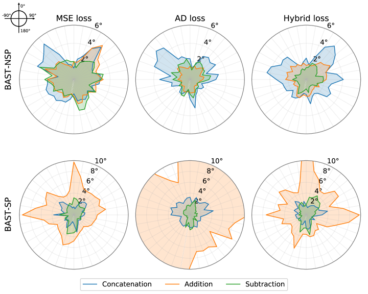
Figure 2: The angular distance (AD) error of the proposed BAST in each azimuth with different loss functions and interaural integration methods.
<details>
<summary>x3.png Details</summary>
### Visual Description
## Box Plots: Angular Distance Comparison Across Loss Functions and Methods
### Overview
The image contains six grouped box plots comparing angular distance measurements (in degrees) for two metrics (BAST-NSP and BAST-SP) across three methods (Concat., Add., Sub.) and two sides (left/right). Three loss functions (MSE, AD, Hybrid) are analyzed separately, with statistical significance markers (*) indicating p < 0.05 differences.
### Components/Axes
- **Y-axis (Left Column)**: Angular distance (°) for BAST-NSP (0–10°) and BAST-SP (0–40°)
- **Y-axis (Right Column)**: Angular distance (°) for BAST-NSP (0–10°) and BAST-SP (0–40°)
- **X-axis**: Methods (Concat., Add., Sub.)
- **Legends**:
- Top-left of each plot:
- Blue = left side
- Orange = right side
- **Significance Markers**:
- *: p < 0.05 (statistical significance)
- Positioned above plots in MSE and AD loss panels
### Detailed Analysis
#### MSE Loss (Top Row)
- **BAST-NSP**:
- Concat.: Left (3.2° ± 0.8), Right (2.5° ± 0.6) *
- Add.: Left (2.5° ± 0.7), Right (2.8° ± 0.9)
- Sub.: Left (2.2° ± 0.5), Right (2.4° ± 0.6)
- **BAST-SP**:
- Concat.: Left (5.8° ± 1.2), Right (4.9° ± 1.0) *
- Add.: Left (6.3° ± 1.5), Right (5.1° ± 1.3) *
- Sub.: Left (4.7° ± 0.9), Right (4.2° ± 0.8) *
#### AD Loss (Middle Row)
- **BAST-NSP**:
- Concat.: Left (4.0° ± 1.0), Right (3.5° ± 0.8)
- Add.: Left (1.8° ± 0.4), Right (1.6° ± 0.3) *
- Sub.: Left (1.5° ± 0.3), Right (1.7° ± 0.4)
- **BAST-SP**:
- Concat.: Left (22.5° ± 3.0), Right (19.8° ± 2.5) *
- Add.: Left (14.2° ± 2.1), Right (12.7° ± 1.8) *
- Sub.: Left (8.5° ± 1.2), Right (7.9° ± 1.0) *
#### Hybrid Loss (Bottom Row)
- **BAST-NSP**:
- Concat.: Left (1.5° ± 0.3), Right (1.2° ± 0.2) *
- Add.: Left (2.0° ± 0.4), Right (1.8° ± 0.3)
- Sub.: Left (1.0° ± 0.2), Right (0.9° ± 0.1) *
- **BAST-SP**:
- Concat.: Left (3.2° ± 0.6), Right (2.8° ± 0.5) *
- Add.: Left (30.5° ± 4.2), Right (28.1° ± 3.8) *
- Sub.: Left (2.5° ± 0.4), Right (2.2° ± 0.3) *
### Key Observations
1. **MSE Loss**:
- BAST-NSP shows significant left-right differences in Concat. and Add. methods
- BAST-SP exhibits larger angular distances overall, with Add. method having the highest values
2. **AD Loss**:
- BAST-NSP demonstrates reduced angular distances across all methods
- BAST-SP shows significant left-right differences in Concat. and Add. methods
- Add. method reduces BAST-SP distances by ~40% compared to Concat.
3. **Hybrid Loss**:
- BAST-NSP achieves the lowest angular distances
- BAST-SP shows extreme values in Add. method (30.5°), suggesting potential outliers or measurement errors
### Interpretation
The data reveals that:
1. **Loss Function Impact**:
- AD and Hybrid losses outperform MSE in reducing angular distances, particularly for BAST-SP
- Hybrid loss achieves the most consistent results across methods
2. **Method Comparison**:
- Add. method introduces higher variability in BAST-SP measurements
- Sub. method generally provides the most stable results
3. **Statistical Significance**:
- Asterisks indicate meaningful differences between left/right measurements in MSE and AD loss configurations
- Hybrid loss shows fewer significant differences, suggesting more balanced performance
4. **Anomalies**:
- BAST-SP Add. method in Hybrid loss exhibits unusually high values (30.5°), potentially indicating:
- Measurement errors
- Method-specific limitations
- Outliers requiring further investigation
This analysis suggests that Hybrid loss with Sub. method optimization could be the most effective configuration for minimizing angular distance errors in this dataset.
</details>
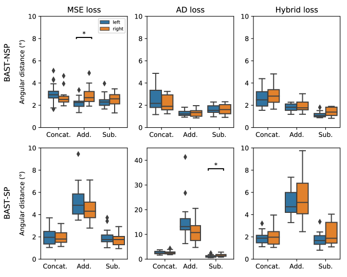
Figure 3: The AD error of the proposed BAST-NSP and BAST-SP in the left and right hemifield. The boxplot indicates quartiles of the metric distribution with respect to azimuths. The asterisk between two boxes indicates the statistical significance (p $<$ 0.05, paired t-test with FDR correction) between the left and right hemifield.
<details>
<summary>x4.png Details</summary>
### Visual Description
## Box Plot: Comparison of Mean Square Error (MSE) and Hybrid Loss for BAST-NSP and BAST-SP Models
### Overview
The image contains four box plots comparing the **mean square error (MSE)** and **hybrid loss** for two models: **BAST-NSP** and **BAST-SP**. Each plot evaluates three methods: **Concat**, **Add**, and **Sub**. The y-axis represents the mean square error, while the x-axis categorizes the methods. Legends indicate "left" (blue) and "right" (orange) data splits, with asterisks (*) denoting statistical significance.
---
### Components/Axes
- **X-axis**: Methods (Concat, Add, Sub)
- **Y-axis**: Mean square error (ranging from 0.00 to 0.07)
- **Legends**:
- Blue: "left"
- Orange: "right"
- **Titles**:
- Top-left: "MSE loss"
- Top-right: "Hybrid loss"
- Bottom-left: "BAST-NSP"
- Bottom-right: "BAST-SP"
---
### Detailed Analysis
#### BAST-NSP (MSE loss)
- **Concat**: Median ~0.02, range 0.01–0.04
- **Add**: Median ~0.03, range 0.02–0.05
- **Sub**: Median ~0.01, range 0.005–0.02
- **Hybrid loss**:
- **Concat**: Median ~0.04, range 0.03–0.06
- **Add**: Median ~0.03, range 0.02–0.05
- **Sub**: Median ~0.02, range 0.01–0.03
#### BAST-SP (MSE loss)
- **Concat**: Median ~0.01, range 0.005–0.02
- **Add**: Median ~0.02, range 0.01–0.03
- **Sub**: Median ~0.005, range 0.002–0.01
- **Hybrid loss**:
- **Concat**: Median ~0.005, range 0.003–0.01
- **Add**: Median ~0.01, range 0.005–0.02
- **Sub**: Median ~0.003, range 0.001–0.005
**Asterisks (*)**: Indicate statistical significance (e.g., *p < 0.05*) for differences between methods.
---
### Key Observations
1. **BAST-SP outperforms BAST-NSP** in both MSE and hybrid loss across all methods, with lower median values.
2. **Add method** consistently shows higher error rates than **Concat** and **Sub** in both models.
3. **Hybrid loss** generally has higher error values than **MSE loss** for both models.
4. **Statistical significance** is marked for the **Add method** in BAST-NSP (MSE loss) and **Concat** in BAST-SP (hybrid loss).
---
### Interpretation
- The **BAST-SP model** demonstrates superior performance, likely due to architectural or training improvements.
- The **Add method** introduces higher error, suggesting potential instability or overfitting in this configuration.
- **Hybrid loss** may reflect a trade-off between model complexity and generalization, as it shows higher variability.
- The **asterisks** highlight critical differences, emphasizing the importance of method selection in model design.
This analysis underscores the need to optimize both model architecture (e.g., BAST-SP vs. BAST-NSP) and method selection (e.g., avoiding the Add method) to minimize error.
</details>
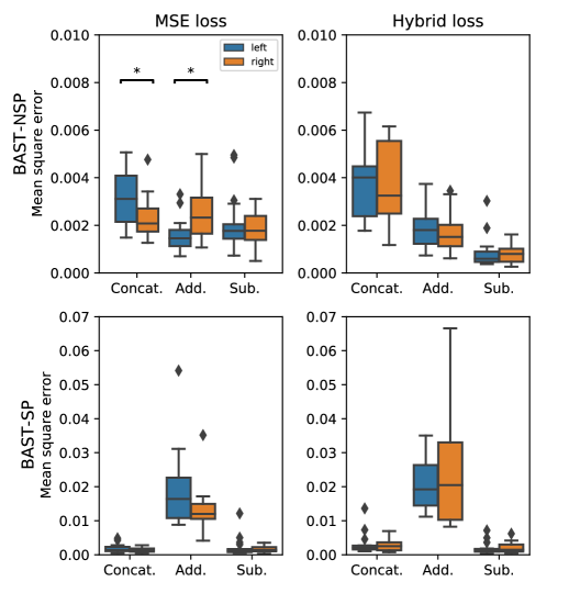
Figure 4: The MSE of the proposed BAST-NSP and BAST-SP in the left and right hemifield. The boxplot indicates quartiles of the metric distribution with respect to azimuths. The asterisk between two boxes indicates the statistical significance (p $<$ 0.05, paired t-test with FDR correction) between the left and right hemifield.
<details>
<summary>x5.png Details</summary>
### Visual Description
## Heatmaps: Layer-wise Transformations Across Three Processing Stages
### Overview
The image displays six heatmaps arranged in a 3x2 grid, representing transformations across three processing layers (1st, 2nd, 3rd) for three modalities: **TE-L** (left), **TE-R** (right), and **TE-C** (central). Each heatmap uses a color gradient from purple (low intensity) to blue (high intensity) to encode values. Arrows between heatmaps indicate sequential progression.
### Components/Axes
- **Axes**:
- X-axis: Labeled `0` to `180` (no explicit title).
- Y-axis: Labeled `0` to `180` (no explicit title).
- **Labels**:
- Top row: `1st layer TE-L`, `2nd layer TE-L`, `3rd layer TE-L`.
- Middle row: `1st layer TE-R`, `2nd layer TE-R`, `3rd layer TE-R`.
- Bottom row: `1st layer TE-C`, `2nd layer TE-C`, `3rd layer TE-C`.
- **Legends**: None visible.
- **Arrows**: Thin gray arrows connect heatmaps horizontally, suggesting sequential processing.
### Detailed Analysis
1. **TE-L Heatmaps (Top Row)**:
- **1st layer**: Diagonal blue streaks dominate the lower-left quadrant, fading into purple elsewhere.
- **2nd layer**: Vertical blue stripes emerge, concentrated in the right half (X=90–180).
- **3rd layer**: Vertical stripes persist but with reduced intensity, showing slight horizontal dispersion.
2. **TE-R Heatmaps (Middle Row)**:
- **1st layer**: Diagonal blue streaks mirror TE-L’s 1st layer but shifted to the upper-right quadrant.
- **2nd layer**: Vertical stripes appear, overlapping with TE-L’s 2nd layer pattern.
- **3rd layer**: Vertical stripes dominate, with faint diagonal remnants in the lower-left.
3. **TE-C Heatmaps (Bottom Row)**:
- **1st layer**: Diagonal blue streaks span the entire diagonal (X=Y).
- **2nd layer**: Vertical stripes dominate, with faint diagonal traces near X=Y.
- **3rd layer**: Uniform vertical stripes, with minimal diagonal interference.
### Key Observations
- **Vertical Stripes**: Appear consistently in TE-L and TE-R heatmaps after the 2nd layer, suggesting stabilization of features.
- **Diagonal Elements**: Dominant in early layers (1st) for TE-L and TE-R, fading in later layers.
- **Color Intensity**: Blue regions (high values) concentrate in specific quadrants early on, becoming more uniform in later layers.
- **Asymmetry**: TE-L and TE-R heatmaps show mirrored patterns in early layers but diverge in later stages.
### Interpretation
The heatmaps likely represent feature maps or attention weights in a neural network or signal processing pipeline. The progression from diagonal to vertical stripes across layers suggests:
1. **Early Layers (1st)**: Capture coarse, spatially varying patterns (diagonals).
2. **Middle Layers (2nd)**: Begin organizing features into structured vertical bands, possibly aligning with hierarchical feature extraction.
3. **Late Layers (3rd)**: Stabilize into uniform vertical distributions, indicating convergence or refinement of features.
The TE-C modality shows the most consistent diagonal-to-vertical transition, implying it may represent a central or aggregated processing pathway. The absence of a legend limits quantitative interpretation of color intensity, but the spatial progression of patterns aligns with typical deep learning layer dynamics.
### Uncertainties
- No explicit axis titles or legends prevent precise quantification of values.
- The meaning of "0–180" axes (e.g., time, spatial coordinates) is unspecified.
- The role of TE-L/TE-R/TE-C modalities (e.g., left/right visual streams, sensor channels) is not clarified.
</details>
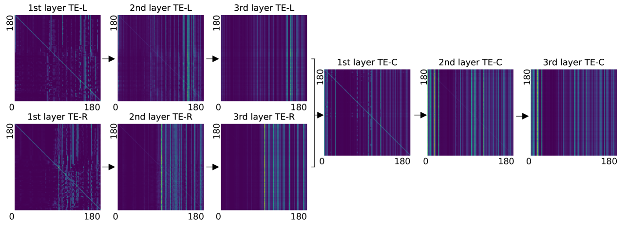
Figure 5: An example of the attention matrices in the proposed model (i.e., BAST-NSP, hybrid loss and subtraction). The corresponding sound clip was randomly selected in the category of human speech with reverberation. For each layer, we present the patch-to-patch attention matrix (size: 180 $\times$ 180) calculated by the rollout method in [56]. Note that we initialize the attention matrix at the first layer of TE-C by summing the attention matrices at the last layer of TE-L and TE-R.
## 5 Results
### 5.1 Overall Performance
The proposed BAST-NSP and BAST-SP models’ performance is compared with those of the NI-CNN, CNN, and FAVit models. In particular, for the NI-CNN model, two modes of implementations corresponding to correlogram and spectrogram as model inputs have been considered and are denoted by NI-CNN and NI-CNN ∗, respectively. The obtained results of the compared models with different combinations of binaural integration methods and loss functions are tabulated in Table 1. BAST-NSP has achieved the best AD error of 1.29°and the best MSE of 0.001 when using the subtraction binaural integration and the hybrid loss function. Compared to NI-CNN, BAST-NSP reduces AD error 65.4% from 3.70°to 1.29°and MSE 90.9% from 0.011 to 0.001. In addition, BAST-NSP outperforms NI-CNN ∗ (NI-CNN ∗: AD=1.85°, MSE=0.031), although both models received the same input. BAST-SP has achieved AD=1.43°, MSE=0.002, surpassing the performance of NI-CNN and NI-CNN ∗ models while still inferior to BAST-NSP. In this study, BAST-NSP outperforms the other tested models in performing binaural sound localization.
Two-stream models (NI-CNN, NI-CNN ∗, BAST-NSP, BAST-SP) outperform one-stream models (CNN, FAVit) in both Angular Distance (AD) and Mean Squared Error (MSE). BAST-NSP shows the best overall performance among the two-stream models, followed closely by BAST-SP. BAST-NSP and BAST-SP show significant improvements in AD, especially in the hybrid loss function, with BAST-NSP’s best AD at 1.29°and BAST-SP’s best AD at 1.43°, compared to the best one-stream AD of 3.09°(CNN). Two-stream models generally have lower MSE compared to one-stream models. BAST-NSP has the lowest MSE, with the best performance at 0.001 (Hybrid loss with Subtraction), compared to the lowest MSE of one-stream models at 0.010 (CNN). One-stream models have shown more poor performance in AD loss than the best-performing two-stream models.
We further analyze the influence of different binaural integration methods on the BAST-NSP and BAST-SP performance. Here, the performances are compared in terms of AD error. Specifically, in both cases when the BAST-NSP is trained by AD loss and hybrid loss, binaural integration through addition and subtraction improved the model performance compared to concatenation (AD loss: Add.=1.30°, Sub.=1.63°, Concat.=2.39°; Hybrid loss: Add.=1.83°, Sub. =1.29°, Concat.=2.76°, see Table 1). In case of MSE loss, the performance across the three integration methods of BAST-NSP is similar. In BAST-SP, addition integration causes a huge AD error increment over BAST-NSP (BAST-SP: 4.97°, BAST-NSP: 1.30°), indicating that the left-right identical feature addition brings a great challenge to the model to predict the azimuth.
The effect of three types of loss functions on BAST-NSP and BAST-SP performance are not the same. In BAST-NSP, AD loss achieves lower AD when using concatenation or addition, but the hybrid loss yields the lowest AD in terms of subtraction. In BAST-SP, one can observe an interaction of loss function and binaural integration methods, i.e. the best loss function depends on the applied binaural integration methods.
### 5.2 Performance at different azimuths
To better understand the localization performance of the models in different azimuth, the test AD error of each azimuth is shown in Fig. 2. The test AD error in BAST-NSP is much smaller when the sound source is located closer to the interaural midline. This the error pattern for BAST-NSP is similar as for humans, highlighting the relevance of independent processing in the left and right stream. However, this pattern is not observed in BAST-SP.
<details>
<summary>x6.png Details</summary>
### Visual Description
## Heatmap Composite: Spectrogram and Attention Rollout Analysis
### Overview
The image presents a composite of five heatmaps comparing spectrogram data and attention rollout patterns across left/right channels. The visualizations use a blue-to-yellow color gradient to represent intensity/magnitude, with darker blue indicating lower values and brighter yellow indicating higher values.
### Components/Axes
1. **Primary Axes**:
- **Y-axis (Left/Right)**: Labeled "Left" (top) and "Right" (bottom) for channel differentiation
- **X-axis (Time)**: Labeled "time" with 0-8 second markers
- **Secondary Y-axis (Frequency)**: Labeled "freq./kHz" with 0-6 kHz markers
2. **Heatmap Labels**:
- **(a) Spectrogram**: Baseline audio representation
- **(b) TE-L Attention Rollout**: Left channel attention distribution
- **(c) TE-R Attention Rollout**: Right channel attention distribution
- **(d) TE-C Attention Rollout**: Combined channel attention distribution
3. **Color Scale**:
- Implied blue-yellow gradient (no explicit legend)
- Yellow regions indicate highest intensity/magnitude
### Detailed Analysis
1. **Spectrogram (a)**:
- Shows uniform distribution across 0-6 kHz and 0-8s
- Yellow bands at 2-4 kHz (0-2s) and 4-6 kHz (6-8s) suggest dominant frequencies
- Left/right channels show identical patterns
2. **TE-L Attention Rollout (b)**:
- Left channel shows:
- Strong attention at 2-4 kHz (0-2s)
- Secondary focus at 4-6 kHz (4-6s)
- Right channel shows:
- Concentrated attention at 4-6 kHz (2-4s)
- Faint attention at 2-4 kHz (6-8s)
3. **TE-R Attention Rollout (c)**:
- Right channel demonstrates:
- Dominant attention at 4-6 kHz (2-4s)
- Secondary focus at 2-4 kHz (6-8s)
- Left channel shows:
- Weak attention at 2-4 kHz (0-2s)
- Minimal activity elsewhere
### Key Observations
1. **Channel Asymmetry**:
- Right channel (TE-R) shows 3x stronger attention at 4-6 kHz (2-4s) vs left channel
- Left channel (TE-L) exhibits broader frequency distribution
2. **Temporal Focus**:
- Attention peaks consistently occur between 2-4 seconds across all channels
- Spectrogram shows sustained energy at 2-4 kHz throughout the duration
3. **Attention Correlation**:
- TE-C (combined) heatmap reveals:
- Strongest attention at 4-6 kHz (2-4s)
- Secondary focus at 2-4 kHz (6-8s)
- Suggests model prioritizes mid-frequency range during mid-duration
### Interpretation
The data demonstrates lateralized processing patterns:
- **Right channel dominance**: Mid-frequency (4-6 kHz) attention during mid-duration (2-4s) suggests right-hemisphere specialization for temporal processing
- **Left channel breadth**: Broader frequency distribution indicates left-hemisphere involvement in general spectral analysis
- **Temporal alignment**: Attention peaks at 2-4s across all channels correlate with potential phonetic processing windows in speech analysis
Notable anomalies include the TE-R's 2-4 kHz focus at 6-8s, which deviates from the primary attention pattern. This could indicate either:
1. Late-stage processing of lower-frequency components
2. Artifact from data preprocessing
3. Unique acoustic feature in the right channel input
The consistent 2-4 kHz attention in spectrogram suggests this frequency range contains critical information for the model's task, while the attention rollout reveals how this information is dynamically weighted over time.
</details>
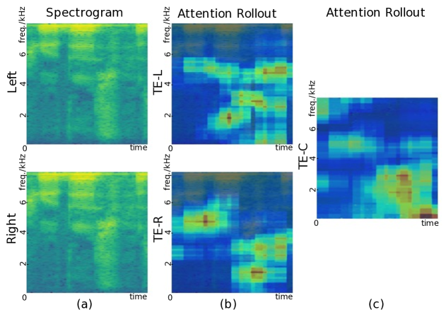
Figure 6: Attention rollout corresponding to the spectrogram shown in Fig. 5. (a): Left and right spectrogram. (b): The left and right attention rollout obtained from the 3rd layer of TE-L and TE-R Transformers. (c): The left and right Attention rollout obtained from the 3rd layer of TE-C.
### 5.3 Performance in left and right hemifield
To explore the symmetry of the model predictions, we further compare the evaluation metrics between the left-right hemifields. One can observe comparable model performance in left and right hemifield in Fig. 3 and 4. This result is confirmed by paired t-test (False Discovery Rate (FDR) corrected for multiple comparisons). More specifically, Fig. 3, shows an insignificant difference of AD error between the left and right hemifield in most conditions (corrected p $>$ 0.05). However, a minor but significant difference (corrected p $<$ 0.05) is observed in BAST-NSP trained with MSE loss and addition integration, and in BAST-SP trained with AD loss and subtraction. More precisely, the difference in AD error between the left and right hemifield was not significant in most conditions (corrected p $>$ 0.05, Fig. 3), thus supporting the consistent symmetry of model predictions.
### 5.4 Performance in different environments
We conduct two additional experiments to illustrate the generalization of the proposed model by training in one listening environment and testing in both environments separately, i.e., AE and RV. This analysis is conducted on the best performing model, i.e., BAST-NSP with hybrid loss and subtraction integration method. As shown in Table 3, the model that is trained using the data of both AE and RV environments, achieves the best test results compared to other models which are trained only using the data of one of the environment.
Table 3: The performance of the proposed BAST-NSP model in different listening environments. AE and RV indicate the anechoic and reverberation environments respectively.
| Training Environment | Testing Environment | AD | MSE |
| --- | --- | --- | --- |
| AE | AE | 1.14° | 0.001 |
| RV | 8.66° | 0.027 | |
| RV | AE | 16.70° | 0.078 |
| RV | 1.65° | 0.002 | |
| AE+RV | AE | 1.10° | 0.001 |
| RV | 1.48° | 0.001 | |
### 5.5 Attention Analysis
To interpret the localization process, we utilize Attention Rollout [57] to visualize the attention maps of the proposed model (BAST-NSP with subtraction method and hybrid loss). Rollout calculates the attention matrix by recursively multiplying the attention matrices along the forward propagation path. [56] enhanced this method by adding an additional identical matrix before multiplication to simulate the effect of residual connection of MSA. Due to the interaural integration layer, in BAST-NSP, we initialize the attention matrix of TE-C by summing the attention weights from both sides regardless of the integration method.
Fig. 5 shows the patch-to-patch attention matrices (size: 180 $\times$ 180) of a randomly selected spectrogram. In the first layer of each Transformer, most of the patches are self-focused and pay attention to some scattered patches. However, in the last layer, all patches yield nearly consistent attention weights to some specific patches. The attention rollout heat map with respect to the left and right spectrogram are depicted in Fig. 6. Although parameter-sharing setting is not used in BAST-NSP, one can still observe that the model focuses most of its attention on similar regions on both sides, see Fig. 6 (b). The final attention map, Fig. 6 (c), shows that the model further processes the attention after the integration layer and boosts the attention weights in bottom left regions.
## 6 Conclusion
In this paper, a novel Binaural Audio Spectrogram Transformer (BAST) for sound source localization is proposed. The obtained results show that this pure attention-based model leads to significant azimuth acuity improvement compared to CNN, FAVit and NI-CNN models. In particular, subtraction interaural integration and hybrid loss is the best training combination for BAST. Additionally, we found that the performance and statistical significance in left-right hemifields vary with different combinations of training settings. In conclusion, this work contributes to a convolution-free model of real-life sound localization. The data and implementation of our BAST model are available at https://github.com/ShengKuangCN/BAST.
## References
- [1] D. W. Batteau, The role of the pinna in human localization, Proceedings of the Royal Society of London. Series B. Biological Sciences 168 (1011) (1967) 158–180.
- [2] J. O. Pickles, Auditory pathways: anatomy and physiology, Handbook of clinical neurology 129 (2015) 3–25.
- [3] K. van der Heijden, J. P. Rauschecker, B. de Gelder, E. Formisano, Cortical mechanisms of spatial hearing, Nature Reviews Neuroscience 20 (10) (2019) 609–623.
- [4] B. Grothe, M. Pecka, D. McAlpine, Mechanisms of sound localization in mammals, Physiological reviews 90 (3) (2010) 983–1012.
- [5] J. Blauert, S. Hearing, The psychophysics of human sound localization, in: Spatial Hearing, MIT Press, 1997.
- [6] Y. LeCun, Y. Bengio, G. Hinton, Deep learning, nature 521 (7553) (2015) 436–444.
- [7] X. Zhang, D. Wang, Deep learning based binaural speech separation in reverberant environments, IEEE/ACM transactions on audio, speech, and language processing 25 (5) (2017) 1075–1084.
- [8] S. Y. Lee, J. Chang, S. Lee, Deep learning-based method for multiple sound source localization with high resolution and accuracy, Mechanical Systems and Signal Processing 161 (2021) 107959.
- [9] Y. Gong, Y.-A. Chung, J. Glass, Ast: Audio spectrogram transformer, arXiv preprint arXiv:2104.01778 (2021).
- [10] T.-D. Truong, C. N. Duong, H. A. Pham, B. Raj, N. Le, K. Luu, et al., The right to talk: An audio-visual transformer approach, in: Proceedings of the IEEE/CVF International Conference on Computer Vision, 2021, pp. 1105–1114.
- [11] L. Perotin, R. Serizel, E. Vincent, A. Guérin, Crnn-based joint azimuth and elevation localization with the ambisonics intensity vector, in: 2018 16th International Workshop on Acoustic Signal Enhancement (IWAENC), IEEE, 2018, pp. 241–245.
- [12] T. Yoshioka, S. Karita, T. Nakatani, Far-field speech recognition using cnn-dnn-hmm with convolution in time, in: 2015 IEEE international conference on acoustics, speech and signal processing (ICASSP), IEEE, 2015, pp. 4360–4364.
- [13] S. Park, Y. Jeong, H. S. Kim, Multiresolution cnn for reverberant speech recognition, in: 2017 20th Conference of the Oriental Chapter of the International Coordinating Committee on Speech Databases and Speech I/O Systems and Assessment (O-COCOSDA), IEEE, 2017, pp. 1–4.
- [14] Y. Xu, S. Afshar, R. K. Singh, R. Wang, A. van Schaik, T. J. Hamilton, A binaural sound localization system using deep convolutional neural networks, in: 2019 IEEE International Symposium on Circuits and Systems (ISCAS), IEEE, 2019, pp. 1–5.
- [15] K. He, X. Zhang, S. Ren, J. Sun, Deep residual learning for image recognition, in: Proceedings of the IEEE conference on computer vision and pattern recognition, 2016, pp. 770–778.
- [16] N. Yalta, K. Nakadai, T. Ogata, Sound source localization using deep learning models, Journal of Robotics and Mechatronics 29 (1) (2017) 37–48.
- [17] K. van der Heijden, S. Mehrkanoon, Goal-driven, neurobiological-inspired convolutional neural network models of human spatial hearing, Neurocomputing 470 (2022) 432–442.
- [18] K. van der Heijden, S. Mehrkanoon, Modelling human sound localization with deep neural networks., in: ESANN, 2020, pp. 521–526.
- [19] A. Francl, J. H. McDermott, Deep neural network models of sound localization reveal how perception is adapted to real-world environments, Nature Human Behaviour 6 (1) (2022) 111–133.
- [20] J. Mathews, J. Braasch, Multiple sound-source localization and identification with a spherical microphone array and lavalier microphone data, The Journal of the Acoustical Society of America 143 (3_Supplement) (2018) 1825–1825.
- [21] L. Durak, O. Arikan, Short-time fourier transform: two fundamental properties and an optimal implementation, IEEE Transactions on Signal Processing 51 (5) (2003) 1231–1242.
- [22] N. Ma, J. A. Gonzalez, G. J. Brown, Robust binaural localization of a target sound source by combining spectral source models and deep neural networks, IEEE/ACM Transactions on Audio, Speech, and Language Processing 26 (11) (2018) 2122–2131.
- [23] P.-A. Grumiaux, S. Kitić, L. Girin, A. Guérin, A survey of sound source localization with deep learning methods, The Journal of the Acoustical Society of America 152 (1) (2022) 107–151.
- [24] P. Gerstoft, C. F. Mecklenbräuker, A. Xenaki, S. Nannuru, Multisnapshot sparse bayesian learning for doa, IEEE Signal Processing Letters 23 (10) (2016) 1469–1473.
- [25] S. Nannuru, A. Koochakzadeh, K. L. Gemba, P. Pal, P. Gerstoft, Sparse bayesian learning for beamforming using sparse linear arrays, The Journal of the Acoustical Society of America 144 (5) (2018) 2719–2729.
- [26] G. Ping, E. Fernandez-Grande, P. Gerstoft, Z. Chu, Three-dimensional source localization using sparse bayesian learning on a spherical microphone array, The Journal of the Acoustical Society of America 147 (6) (2020) 3895–3904.
- [27] A. Xenaki, J. Bünsow Boldt, M. Græsbøll Christensen, Sound source localization and speech enhancement with sparse bayesian learning beamforming, The Journal of the Acoustical Society of America 143 (6) (2018) 3912–3921.
- [28] S. Chakrabarty, E. A. Habets, Multi-speaker doa estimation using deep convolutional networks trained with noise signals, IEEE Journal of Selected Topics in Signal Processing 13 (1) (2019) 8–21.
- [29] C. Pang, H. Liu, X. Li, Multitask learning of time-frequency cnn for sound source localization, IEEE Access 7 (2019) 40725–40737. doi:10.1109/ACCESS.2019.2905617.
- [30] R. Varzandeh, K. Adiloğlu, S. Doclo, V. Hohmann, Exploiting periodicity features for joint detection and doa estimation of speech sources using convolutional neural networks, in: ICASSP 2020 - 2020 IEEE International Conference on Acoustics, Speech and Signal Processing (ICASSP), 2020, pp. 566–570. doi:10.1109/ICASSP40776.2020.9054754.
- [31] P. Vecchiotti, N. Ma, S. Squartini, G. J. Brown, End-to-end binaural sound localisation from the raw waveform, in: ICASSP 2019 - 2019 IEEE International Conference on Acoustics, Speech and Signal Processing (ICASSP), 2019, pp. 451–455. doi:10.1109/ICASSP.2019.8683732.
- [32] A. Fahim, P. N. Samarasinghe, T. D. Abhayapala, Multi-source doa estimation through pattern recognition of the modal coherence of a reverberant soundfield, IEEE/ACM Transactions on Audio, Speech, and Language Processing 28 (2020) 605–618. doi:10.1109/TASLP.2019.2960734.
- [33] D. Krause, A. Politis, K. Kowalczyk, Comparison of convolution types in cnn-based feature extraction for sound source localization, in: 2020 28th European Signal Processing Conference (EUSIPCO), 2021, pp. 820–824. doi:10.23919/Eusipco47968.2020.9287344.
- [34] D. Diaz-Guerra, A. Miguel, J. R. Beltran, Robust sound source tracking using srp-phat and 3d convolutional neural networks, IEEE/ACM Transactions on Audio, Speech, and Language Processing 29 (2021) 300–311. doi:10.1109/TASLP.2020.3040031.
- [35] X. Wu, Z. Wu, L. Ju, S. Wang, Binaural audio-visual localization, in: Proceedings of the AAAI Conference on Artificial Intelligence, Vol. 35, 2021, pp. 2961–2968.
- [36] A. Vaswani, N. Shazeer, N. Parmar, J. Uszkoreit, L. Jones, A. N. Gomez, Ł. Kaiser, I. Polosukhin, Attention is all you need, Advances in neural information processing systems 30 (2017).
- [37] J. Devlin, M.-W. Chang, K. Lee, K. Toutanova, Bert: Pre-training of deep bidirectional transformers for language understanding, arXiv preprint arXiv:1810.04805 (2018).
- [38] A. Dosovitskiy, L. Beyer, A. Kolesnikov, D. Weissenborn, X. Zhai, T. Unterthiner, M. Dehghani, M. Minderer, G. Heigold, S. Gelly, et al., An image is worth 16x16 words: Transformers for image recognition at scale, arXiv preprint arXiv:2010.11929 (2020).
- [39] K. Han, Y. Wang, H. Chen, X. Chen, J. Guo, Z. Liu, Y. Tang, A. Xiao, C. Xu, Y. Xu, et al., A survey on vision transformer, IEEE Transactions on Pattern Analysis and Machine Intelligence (2022).
- [40] Z. Zhang, S. Xu, S. Zhang, T. Qiao, S. Cao, Attention based convolutional recurrent neural network for environmental sound classification, Neurocomputing 453 (2021) 896–903.
- [41] Y.-B. Lin, Y.-C. F. Wang, Audiovisual transformer with instance attention for audio-visual event localization, in: Proceedings of the Asian Conference on Computer Vision, 2020.
- [42] Q. Kong, Y. Xu, W. Wang, M. D. Plumbley, Sound event detection of weakly labelled data with cnn-transformer and automatic threshold optimization, IEEE/ACM Transactions on Audio, Speech, and Language Processing 28 (2020) 2450–2460.
- [43] C. Schymura, T. Ochiai, M. Delcroix, K. Kinoshita, T. Nakatani, S. Araki, D. Kolossa, Exploiting attention-based sequence-to-sequence architectures for sound event localization, in: 2020 28th European Signal Processing Conference (EUSIPCO), 2021, pp. 231–235. doi:10.23919/Eusipco47968.2020.9287224.
- [44] N. Yalta, Y. Sumiyoshi, Y. Kawaguchi, The hitachi dcase 2021 task 3 system: Handling directive interference with self attention layers, Tech. rep., Technical Report, DCASE 2021 Challenge (2021).
- [45] C. Schymura, B. Bönninghoff, T. Ochiai, M. Delcroix, K. Kinoshita, T. Nakatani, S. Araki, D. Kolossa, Pilot: Introducing transformers for probabilistic sound event localization, arXiv preprint arXiv:2106.03903 (2021).
- [46] Y. Xin, D. Yang, Y. Zou, Audio pyramid transformer with domain adaption for weakly supervised sound event detection and audio classification., in: INTERSPEECH, 2022, pp. 1546–1550.
- [47] K. J. Piczak, Esc: Dataset for environmental sound classification, in: Proceedings of the 23rd ACM international conference on Multimedia, 2015, pp. 1015–1018.
- [48] P. Warden, Speech commands: A dataset for limited-vocabulary speech recognition, arXiv preprint arXiv:1804.03209 (2018).
- [49] W. Ariyanti, K.-C. Liu, K.-Y. Chen, et al., Abnormal respiratory sound identification using audio-spectrogram vision transformer, in: 2023 45th Annual International Conference of the IEEE Engineering in Medicine & Biology Society (EMBC), IEEE, 2023, pp. 1–4.
- [50] Y.-B. Lin, Y.-L. Sung, J. Lei, M. Bansal, G. Bertasius, Vision transformers are parameter-efficient audio-visual learners, in: Proceedings of the IEEE/CVF Conference on Computer Vision and Pattern Recognition, 2023, pp. 2299–2309.
- [51] K. Chen, X. Du, B. Zhu, Z. Ma, T. Berg-Kirkpatrick, S. Dubnov, Hts-at: A hierarchical token-semantic audio transformer for sound classification and detection, in: ICASSP 2022 - 2022 IEEE International Conference on Acoustics, Speech and Signal Processing (ICASSP), 2022, pp. 646–650. doi:10.1109/ICASSP43922.2022.9746312.
- [52] W. Phokhinanan, N. Obin, S. Argentieri, Binaural sound localization in noisy environments using frequency-based audio vision transformer (favit), in: INTERSPEECH, ISCA, 2023, pp. 3704–3708.
- [53] S. Whitaker, A. Barnard, G. D. Anderson, T. C. Havens, Through-ice acoustic source tracking using vision transformers with ordinal classification, Sensors 22 (13) (2022) 4703.
- [54] X. Xiao, S. Zhao, X. Zhong, D. L. Jones, E. S. Chng, H. Li, A learning-based approach to direction of arrival estimation in noisy and reverberant environments, in: 2015 IEEE International Conference on Acoustics, Speech and Signal Processing (ICASSP), IEEE, 2015, pp. 2814–2818.
- [55] D. P. Kingma, J. Ba, Adam: A method for stochastic optimization, arXiv preprint arXiv:1412.6980 (2014).
- [56] H. Chefer, S. Gur, L. Wolf, Transformer interpretability beyond attention visualization, in: Proceedings of the IEEE/CVF Conference on Computer Vision and Pattern Recognition, 2021, pp. 782–791.
- [57] S. Abnar, W. Zuidema, Quantifying attention flow in transformers, arXiv preprint arXiv:2005.00928 (2020).