2207.06405v3

# Masked Autoencoders that Listen **Authors**: Po-Yao Huang, Hu Xu, Juncheng Li, Alexei Baevski, Michael Auli, Wojciech Galuba, Florian Metze, Christoph Feichtenhofer ## Masked Autoencoders that Listen Po-Yao Huang 1 Hu Xu 1 Juncheng Li 2 Alexei Baevski 1 Michael Auli 1 Wojciech Galuba 1 Florian Metze 1 Christoph Feichtenhofer 1 1 Meta AI 2 Carnegie Mellon University ## Abstract This paper studies a simple extension of image-based Masked Autoencoders (MAE) [1] to self-supervised representation learning from audio spectrograms. Following the Transformer encoder-decoder design in MAE, our Audio-MAE first encodes audio spectrogram patches with a high masking ratio, feeding only the non-masked tokens through encoder layers. The decoder then re-orders and decodes the encoded context padded with mask tokens, in order to reconstruct the input spectrogram. We find it beneficial to incorporate local window attention in the decoder, as audio spectrograms are highly correlated in local time and frequency bands. We then fine-tune the encoder with a lower masking ratio on target datasets. Empirically, Audio-MAE sets new state-of-the-art performance on six audio and speech classification tasks, outperforming other recent models that use external supervised pre-training. Our code and models is available at https://github.com/facebookresearch/AudioMAE . ## 1 Introduction Transformers [2] and self-supervised learning [3, 4, 5, 6, 7, 1] are dominating computer vision (CV) and natural language processing (NLP) research. The revolution firstly started in NLP with the invention of the Transformer architecture and self-attention [8]. Masked autoencoding with BERT [3] set a new state-of-the-art on various NLP tasks by self-supervised pre-training on large-scale language corpus. Similarly in the CV community, Vision Transformers (ViT) [9] have become popular for CV tasks, and, for self-supervised image representation learning, Masked Autoencoders (MAE) [1] have brought the CV community closer to the success of BERT in NLP. In addition to the existing masked autoencoders that can read (BERT) or see (MAE), in this work we study those that can listen . Transformer-based models have recently refreshed leaderboards for audio understanding tasks. For example, AST [10] and MBT [11] improved the audio classification performance on the AudioSet [12], Event Sound Classification [13], etc. The key technique behind this is initialization of audio model weights with ImageNet pre-trained supervised models ( e.g ., DeiT [14]) by deflating patch embeddings and interpolating positional embeddings for encoding audio spectrograms. However, exploiting ImageNet pre-trained models could be sub-optimal. Unlike initializing video models with weights from image models ( e.g ., the initial weights of I3D [15] or 3D-ResNets [16] are inflated from ImageNet pre-trained image models), there are clear and notable discrepancies between spectrograms representing audio content and natural images. It remains unclear why such heterogeneous image-toaudio transfer is useful beyond arguably similar low-level semantics such as shapes of spectrograms and shapes of visual objects. Further, any label bias would inevitably be transferred to audio models. Addressing these concerns, self-supervised audio representation learning has recently attracted much research attention. Based on BEiT [17] that learns to reconstruct image patches or learnt patch tokens, SS-AST [18] extends to the audio domain and exploits spectrograms (akin to 1-channel 2D images) and use both contrastive and reconstruction objective as self-supervision. Without using any labels, the key enabler to effective self-supervised representation learning is large-scale pre-training data. In this work we use AudioSet [12] for pre-training, a common dataset containing ∼ 2 million audio recordings. Performing large-scale training with Transformer architectures is challenging as self-attention in Transformers has quadratic complexity w.r.t. the length of input sequence. 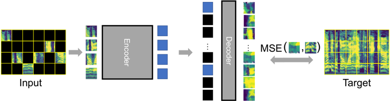Figure 1: Audio-MAE for audio self-supervised learning . An audio recording is first transformed into a spectrogram and split into patches. We embed patches and mask out a large subset (80%). An encoder then operates on the visible (20%) patch embeddings. Finally, a decoder processes the order-restored embeddings and mask tokens to reconstruct the input. Audio-MAE is minimizing the mean square error (MSE) on the masked portion of the reconstruction and the input spectrogram. <details> <summary>Image 1 Details</summary>  ### Visual Description ## Diagram: Autoencoder Architecture with Reconstruction Loss ### Overview The diagram illustrates the flow of data through an autoencoder architecture, demonstrating how input data is compressed, reconstructed, and evaluated for quality. The process includes an encoder, decoder, and mean squared error (MSE) loss function to quantify reconstruction accuracy. ### Components/Axes 1. **Input**: A 4x4 grid of patches with varying color intensities (black, blue, green, yellow). Some patches are fully colored, while others are partially filled or empty. 2. **Encoder**: A gray rectangular block labeled "Encoder," representing the dimensionality reduction phase. It processes the input into a compressed representation (blue squares). 3. **Decoder**: A gray rectangular block labeled "Decoder," responsible for reconstructing the input from the compressed representation. It outputs a grid of patches similar to the input. 4. **Target**: A 4x4 grid of patches with distinct color distributions compared to the input, serving as the ground truth for reconstruction. 5. **MSE (Mean Squared Error)**: A bidirectional arrow labeled "MSE" connecting the decoder output to the target, indicating the loss function used to optimize the model. ### Detailed Analysis - **Input**: The input grid contains 16 patches. Approximately 6 patches are fully colored (mix of blue, green, yellow), 4 patches are partially filled, and 6 patches are empty (black). The spatial arrangement suggests localized features. - **Encoder**: Converts the input into a compressed representation (blue squares). The exact dimensions of the compressed representation are not specified but are implied to be smaller than the input. - **Decoder**: Expands the compressed representation back into a grid format. The decoder output matches the input's 4x4 structure but with altered patch distributions. - **Target**: The target grid has 16 patches with a different spatial distribution of colors. Approximately 8 patches are fully colored (predominantly yellow and green), 5 patches are partially filled, and 3 patches are empty. This differs significantly from the input grid. - **MSE**: The bidirectional arrow indicates that the MSE loss is calculated between the decoder's output and the target. This loss drives the optimization of the encoder-decoder parameters to minimize reconstruction error. ### Key Observations 1. **Input vs. Target Discrepancy**: The input and target grids differ in patch distribution, suggesting the autoencoder is trained to reconstruct a target that may not match the original input (e.g., denoising or anomaly detection). 2. **Encoder Compression**: The encoder reduces the input's spatial complexity into a lower-dimensional representation (blue squares), critical for learning efficient features. 3. **Decoder Reconstruction**: The decoder attempts to recover the target structure from the compressed representation, highlighting the model's ability to generalize. 4. **MSE as Optimization Driver**: The MSE loss quantifies the difference between reconstructed and target outputs, guiding the training process to improve accuracy. ### Interpretation This diagram demonstrates the core functionality of an autoencoder: learning a compressed representation of data (via the encoder) and reconstructing it (via the decoder) while minimizing reconstruction error (MSE). The mismatch between input and target implies the model could be used for tasks like: - **Denoising**: Reconstructing clean data from noisy inputs. - **Anomaly Detection**: Identifying inputs where the reconstruction error (MSE) exceeds a threshold. - **Dimensionality Reduction**: Efficiently encoding high-dimensional data into a latent space. The use of MSE as the loss function emphasizes the importance of pixel-level accuracy in reconstruction, which is critical for applications requiring precise output matching (e.g., image restoration). The colored patches likely represent features the model learns to capture, with the encoder-decoder architecture balancing compression and fidelity. </details> This computational burden has been addressed in different ways. A popular approach is to reduce the sequence length in self-attention. Various ViT-based architectures have been developed to alleviate such issues for image and video understanding. For example, Swin-Transformer [19] only performs local attention within windows that shift across layers. MViT [20] employs pooling attention to construct a hierarchy of Transformers where sequence lengths are downsampled. For self-supervised learning, MAE [1] efficiently encodes only a small portion (25%) of visual patches while the majority of patches is discarded. The simplicity and scalability in MAE make it a promising framework for large-scale self-supervised learning. In this work, we study MAE for sound recognition and the unique challenges of the audio domain. We present Audio-MAE (Fig. 1) as unified and scalable framework for learning self-supervised audio representations. Similar to MAE, it is composed of a pair of a Transformer encoder and decoder. Sound is first transformed and embedded into spectrogram patches. Before feeding them into the Transformer encoder, we mask and discard the majority and only feed a small number of non-masked embeddings into the encoder for efficient encoding. After padding encoded patches with learnable embeddings to represent masked patches, it then restores the order of these patches in frequency and time and propagates them through a Transformer decoder to reconstruct the audio spectrogram. Different from image patches, spectrogram patches are comparably local-correlated. For example, formants, the vocal tract resonances, are typically grouped and continuous locally in the spectrogram. The location in frequency and time embeds essential information that determines the semantics of a spectrogram patch and how it sounds like. To this end, we further investigate using localized attention and a hybrid architecture in the Transformer decoder to properly decode for reconstruction. This simple-yet-effective upgrade leads to improved performance for Audio-MAE. Similar to MAE for images, we minimize the patch-normalized mean square error. At the fine-tuning stage, we discard the decoder and fine-tune the encoder with patch-masking. Empirically, AudioMAEsets a new state-of-the-art performance on six audio and speech classification tasks. It is the first audio-only self-supervised model that achieves state-of-the-art mAP on AudioSet-2M, outperforming other recent models with external supervision. We further provide the visualization and audible examples to qualitatively demonstrate the effectiveness of the Audio-MAE decoder. ## 2 Related Work Visual masked pre-training. Masked/Denoising autoencoders [21, 22, 3] are a general representation learning methodology by reconstructing source from masked or corrupted inputs. In CV, visual masked pre-training has made recent progress [23, 24, 1, 20]. Based on ViT [9] that applies Transformers to image patches, BEiT [17] and MAE [1] present masked image modeling frameworks. BEiT [17] learns to predict discrete visual tokens generated by V AE [25] in masked patches. MAE [1] reduces sequence length by masking a large portion of image patches randomly and encoding only non-masked ones for reconstruction of pixel color information. MaskFeat [20] studies features for masked pre-training and finds that Histograms of Oriented Gradients (HoG) [26], which are in turn related to spectrogram features, perform strongly for image and video classification models. Our work extends the MAE framework for representation learning with audio spectrograms. Out-of-domain pre-training for audio. Transferring ImageNet supervised pre-trained ViT [9] or ResNet [27] has become a popular practice for audio models [10, 28, 11, 29, 30, 31]. After pre-training, these models operate over audio spectrograms by deflating from 3-channels (RGB) into 1-channel (spectrogram) in the pre-trained patch embedding in ViT and employing the rest of the transformer blocks on top. For example, HTS-AT [29] encodes spectrograms with hierarchical Transformer initialized from the Swin Transformer [19]. MBT [11] uses ImageNet-21K pre-trained ViT; AST [10] and PaSST [28] employ DeiT [14] as the Transformer backbone. Without using out-of-domain (non-audio) data, the proposed Audio-MAE focuses on audio-only self-supervised pre-training from scratch. In-domain pre-training for audio. Existing in-domain ( i.e ., audio-only) self-supervised methods can be broadly categorized by the input signal type ( e.g ., raw waveform [32, 33, 34], frame-level features [35, 36, 37], or spectrogram patches [18, 38]); and the objective used for self-supervision ( e.g ., contrastive [39, 33, 40, 41, 35] or prediction/reconstruction [18, 34, 37, 36]). For example, wav2vec 2.0 [33] takes raw waveform as inputs and exploits contrastive learning to discriminate contextualized representations in different time segments. Mockingjay [42] proposed a masked acoustic model pretext task to reconstruct frame-level Mel-features of masked time frames. SSAST [18] is the closest work to Audio-MAE and is our main benchmark. Inspired by the success of BERT [3], SS-AST proposed a self-supervised learning method which operates over spectrogram patches and employs joint contrastive and reconstructive objectives on masked patches. These previous methods generate audio representations by encoding full-view of both masked and nonmasked time or spectrogram segments for self-supervised pre-training. In contrast, Audio-MAE encodes only the non-masked spectrogram patches. Our work is done independently and concurrently with [38, 43, 44] related methods. We also compare our model to these concurrent works in the experiments and showcase the superiority of Audio-MAE. ## 3 Audio Masked Autoencoders (Audio-MAE) Audio-MAE is a conceptually simple extension of MAE to learn self-supervised representations from audio spectrograms. Fig. 1 depicts an overview. The details of each component are as follows. Spectrogram Patch Embeddings . Following [10, 18], we transform audio recordings into Melspectrograms and divide them into non-overlapped regular grid patches. These patches are then flattened and embedded by a linear projection. Similar to MAE [1], we add fixed sinusoidal positional embeddings to the embedded patches. Figure 2: Audio-MAE's masking strategies on Mel-spectrograms. <details> <summary>Image 2 Details</summary>  ### Visual Description ## Heatmap Visualization: Spectrogram Masking Patterns ### Overview The image displays five heatmap panels (a-e) comparing different masking strategies applied to a spectrogram. Each panel uses a color gradient (yellow-green-blue) to represent signal intensity, with black regions indicating masked areas. The panels demonstrate progressive masking techniques from unstructured to structured patterns. ### Components/Axes - **Panels**: - (a) Original: Full spectrogram with no masking - (b) Unstructured: Checkerboard pattern masking - (c) Time: Vertical stripe masking - (d) Frequency: Horizontal stripe masking - (e) Time+frequency: Combined vertical/horizontal masking - **Axes**: - Implied time axis (x-axis) and frequency axis (y-axis) based on spectrogram conventions - No explicit axis labels or scales visible - **Color Scale**: - Yellow (high intensity) to blue (low intensity) - No numerical legend present ### Detailed Analysis 1. **Panel (a) Original**: - Full spectrogram with continuous color gradients - Vertical striations suggest periodic signals - Horizontal bands indicate frequency components 2. **Panel (b) Unstructured**: - 50% checkerboard masking (alternating black/white blocks) - Random spatial distribution of masked regions - Preserves some temporal and frequency continuity 3. **Panel (c) Time**: - Vertical black stripes mask 30-40% of time axis - Regular 10-unit interval masking pattern - Frequency components remain fully visible 4. **Panel (d) Frequency**: - Horizontal black stripes mask 25% of frequency axis - Regular 8-unit interval masking pattern - Temporal continuity preserved 5. **Panel (e) Time+frequency**: - Overlapping vertical/horizontal masking - Creates grid-like occlusion pattern - 60% of data points masked in combined pattern ### Key Observations - Masking intensity increases from (a) to (e) - Structured masking (c-d) shows systematic data removal - Combined masking (e) creates diagonal artifacts - Color gradients remain consistent across panels - No explicit numerical values or units provided ### Interpretation This visualization demonstrates the impact of different masking strategies on spectrogram analysis: 1. **Structured vs Unstructured**: Checkerboard masking (b) preserves more contextual information than structured time/frequency masking 2. **Temporal vs Frequency Focus**: Vertical masking (c) disrupts time-domain analysis more than horizontal masking (d) affects frequency analysis 3. **Combined Effects**: Panel (e) shows how simultaneous time/frequency masking creates unique artifacts not present in single-axis masking 4. **Signal Robustness**: The original spectrogram (a) reveals complex periodic patterns that become increasingly obscured in masked versions The progression suggests this could be used to evaluate machine learning models' ability to handle partial data or to study human perception of masked audio signals. The absence of explicit legends/axes implies this is a conceptual demonstration rather than quantitative analysis. </details> Masking Strategies . Audio-MAE masks out a large subset of spectrogram patches. As a spectrogram can be viewed as a 2D representation of time and frequency components of a sound, it is reasonable to explore treating time and frequency differently during masking. In this work, we investigate both the unstructured ( i.e ., random masking without any prior) and structured ( i.e ., randomly masking a portion of time, frequency, or time + frequency of a spectrogram) in the pre-training and fine-tuning phase. Illustrative examples are shown in Fig. 2. We show masked regions with dark overlay. The masking mechanism, as introduced in MAE [1], is the key ingredient for efficient self-supervised learning. For a input patch sequence, this can be regarded as a Bernoulli process where each patch is masked/dropped with probability p (masking ratio). Masking reduces input patch sequence length and encourages learning global, contextualized representations from limited 'visible' patches. We observe that akin to images, a large masking rate (80% in our experiments for spectrogram patches, which is similar to 75% in MAE for images) is feasible for learning self-supervised audio representations. Unlike BERT [3] that uses 15% masking rate for self-supervised learning in NLP, most of the tokens/patches can be discarded for spectrograms as well as images due to high redundancy in these modalities. Beyond self-supervised pre-training, we further explore the effectiveness of masking in the supervised fine-tuning stage. Empirically, we found unstructured (random) masking at a higher ratio for pre-training and structured (time + frequency masking) at a lower ratio for fine-tuning provide best accuracy (ablations are in §4.4). Encoder . Audio-MAE uses a stack of standard Transformers [2] as its encoder. The encoder only processes (20%) non-masked patches to reduce computation overhead which is quadratic to the input sequence length. We use the 12-layer ViT-Base (ViT-B) [9] Transformer as our default. Decoder with Local Attention . The decoder is also composed of standard Transformer blocks. The encoded patches from the encoder are padded with trainable masked tokens. After restoring the original time-frequency order in the audio spectrogram, we add the decoder's (fixed sinusoidal) positional embeddings and feed the restored sequence into the decoder. At the top of the decoder stack, we add a linear head to predict and reconstruct the input spectrogram. To address the unique characteristics of audio spectrograms, our work investigates an enhancement to the vanilla MAE decoder. Image-based MAE uses global self-attention in the Transformer decoder which is appropriate for visual context, because visual objects are typically invariant under translation or scaling, and their exact position may not affect the semantics of an image. In contrast, the position, scale, and translation of spectrogram features however directly affects the sound or semantics of an audio recording. Consequently, global self-attention is sub-optimal for spectrograms if the timefrequency components is predominantly local. For instance, we would have better success to use the harmonics ( e.g ., Fig. 2a) in lower bands of a vowel to predict the spectrogram patch vertically in a higher frequency band rather than horizontally in the time domain. Similarly, a frictional sound of a consonant likely only correlates to other part of the consonant, and is without dependency to other silence segments in the audio recording. Compared to images, the spectrogram patches are more similar to speech or text tokens where its order and position is more relevant. 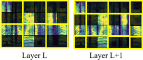To address the nature of audio spectrograms, in addition to using Transformers with global self-attention as in vanilla MAE, we incorporate the local attention mechanism which groups and separates the spectrogram patches in to local windows in self-attention for decoding. We investigate two types of local attention: (1) Shifted window location: Inspired by the shifted-window in Swin Transformers [19], we shift window attention by 50% between consecutive Transformer decoder layers. For padding the margin when shifting, we cyclically shift the spectrogram to the top-left direction. Fig. 3 illustrates Figure 3: Decoder's local attention and shifted window (right). <details> <summary>Image 3 Details</summary>  ### Visual Description ## Heatmap Visualization: Layer L vs Layer L+1 ### Overview The image presents two side-by-side heatmaps labeled "Layer L" (left) and "Layer L+1" (right), each divided into a 3x3 grid of cells. Both heatmaps use a color gradient ranging from dark green (low values) to yellow (medium) to blue (high values). The grids are outlined with yellow borders, and the labels are positioned at the bottom center of each heatmap. --- ### Components/Axes - **Labels**: - "Layer L" (bottom-left heatmap) - "Layer L+1" (bottom-right heatmap) - **Grid Structure**: - Both heatmaps contain 9 cells arranged in 3 rows and 3 columns. - No explicit axis titles or numerical scales are visible. - **Color Gradient**: - Dark green → Yellow → Blue (inferred intensity scale, no legend present). - **Positioning**: - Heatmaps are aligned horizontally, with "Layer L" on the left and "Layer L+1" on the right. - Labels are centered below their respective heatmaps. --- ### Detailed Analysis #### Layer L (Left Heatmap) - **Top Row**: - Left cell: Predominantly dark green (low values). - Middle cell: Mix of dark green and yellow (moderate variation). - Right cell: Dark green with faint yellow streaks. - **Middle Row**: - Left cell: Vertical yellow streaks on dark green background. - Middle cell: Horizontal yellow streaks with dark green base. - Right cell: Vertical yellow streaks with dark green base. - **Bottom Row**: - Left cell: Dark green with faint yellow horizontal lines. - Middle cell: Dark green with faint vertical yellow lines. - Right cell: Dark green with faint diagonal yellow lines. #### Layer L+1 (Right Heatmap) - **Top Row**: - Left cell: Vertical yellow streaks on dark green. - Middle cell: Horizontal yellow streaks with dark green base. - Right cell: Vertical yellow streaks with dark green base. - **Middle Row**: - Left cell: Horizontal yellow streaks with dark green base. - Middle cell: Dominant yellow with dark green base. - Right cell: Vertical yellow streaks with dark green base. - **Bottom Row**: - Left cell: Vertical yellow streaks with dark green base. - Middle cell: Horizontal yellow streaks with dark green base. - Right cell: Vertical yellow streaks with dark green base. --- ### Key Observations 1. **Layer L+1 shows higher overall intensity**: - More cells in Layer L+1 exhibit yellow/blue hues compared to Layer L. - Example: The middle row of Layer L+1 has two cells with dominant yellow, while Layer L’s middle row has only one. 2. **Bottom-right cell divergence**: - Layer L’s bottom-right cell has faint diagonal yellow lines on dark green. - Layer L+1’s bottom-right cell shows vertical yellow streaks, indicating a significant increase in activity. 3. **Middle row trend**: - Layer L+1’s middle row has a consistent yellow streak pattern, suggesting a systematic change or activation. 4. **Color consistency**: - Dark green dominates Layer L, while Layer L+1 shifts toward yellow/blue, implying a progression or transformation between layers. --- ### Interpretation The heatmaps likely represent feature maps or activation patterns in a neural network, where Layer L+1 builds upon Layer L. The increased yellow/blue intensity in Layer L+1 suggests enhanced feature extraction or activation in specific regions. The middle row’s consistent yellow streaks in Layer L+1 may indicate a localized transformation or pooling operation. The bottom-right cell’s dramatic shift from faint diagonal lines (Layer L) to vertical streaks (Layer L+1) could represent a critical feature amplification or edge detection. The absence of a legend limits precise quantification, but the relative color intensity differences highlight a clear progression between layers. </details> the localized decoder attention by shifted windows. (2) Hybrid window attention (global + local attention): Inspired by [45], to add better cross-window connections, we design a simple hybrid (global+local) attention that computes local attention within a window in all but the last few top layers. In this way, the input feature maps for the final reconstruction layer also contain global information. For simplicity, we use no pooling or hierarchical structure. Decoders with different attention types are compared in §4.4. Objective . The Audio-MAE decoder learns to reconstruct the input spectrogram by predicting the values in the spectrogram patches or their per-patch normalized ones. The objective is the mean squared error (MSE) between the prediction and the input spectrogram, averaged over unknown patches. Empirically we found employing the reconstruction loss alone is sufficient while including additional contrastive objectives ( e.g ., InfoNCE loss [46]) does not improve Audio-MAE. Fine-tuning for Downstream Tasks . In the fine-tuning stage, we only keep and fine-tune the AudioMAE encoder and discard the decoder. Different from the original MAE, and inspired by [47, 28], we also explore to employ masking in the fine-tuning stage to remove a portion of patches to further regularize learning from a limited view of spectrogram inputs, which, as a side effect, also reduces computation during fine-tuning. Compared to SpecAug [48] which takes full-length input with the masked portion set to zero as data augmentation, Audio-MAE sees only a subset of real-valued input patches without the nullified ones. Audio-MAE then encodes these non-masked patches and applies an average pooling layer followed by a linear layer on top for fine-tuning in classification tasks. ## 4 Experiments We perform an extensive evaluation on six tasks, including audio classification on AudioSet (AS-2M, AS-20K) and Environmental Sound Classification (ESC-50), and speech classification on Speech Commands (SPC-1 and SPC-2) and VoxCeleb (SID). We use AudioSet for ablation studies. ## 4.1 Datasets and Tasks AudioSet [12] (AS-2M, AS-20K) contains ∼ 2 million 10-second YouTube clips for audio classification. 527 types of audio events are weakly annotated [49, 50, 51] for each clip. There could be multiple events in a clip. The full training set has 2 subsets: A class-wise balanced (22,176 clips) and an unbalanced (2,042,985 clips) set. The eval set has 20,383 clips. We downloaded and processed around 1.96M unbalanced training, 21K balanced training, and 19K evaluation clips. For the AS-2M experiments, we use the union of unbalanced and balanced training audio for pretraining and fine-tuning. For the AS-20K experiments, we use AS-2M for pre-training and the 20K balanced set for fine-tuning. We report the testing mAP on the 19K eval set used by AST [10]. Environmental Sound Classification (ESC-50) [13] is an audio classification dataset consists of 2,000 5-second environmental sound recordings. There are 50 classes in ESC. We report accuracy under 5-fold cross-validation with the same split used by [10]. Speech Commands (SPC-2, SPC-1) [52] are two keyword spotting tasks. In SPC-2, there are 35 speech commands. The training/validation/testing set has 84,843/9,981/11,005 1-second recordings, respectively. In SPC-1, there are 10 classes of keywords, 1 silence class, and 1 unknown class that includes all the other 20 common speech commands. We use the data and split provided in the SUPERB [53] benchmark to report the testing accuracy. VoxCeleb (SID) [54] contains 150K utterances from 1,251 speakers. The speaker identification task (SID) is to classify the utterances to identify its original speaker. We use the V1 standard train (138,361), validation (6,904), testing (8,251) sets and report the testing accuracy. ## 4.2 Implementation Details We use a vanilla 12-layer ViT-B by default as the Transformer encoder. For the decoder, we use a 16-layer Transformer with shifted local attention. We investigate the vanilla (global attention) and hybrid (global + local attention) decoder variants (see Table. 1c). Following [10, 11], we transform raw waveform (pre-processed as mono channel under 16,000 sampling rate) into 128 Kaldi [55]-compatible Mel-frequency bands with a 25ms Hanning window that shifts every 10 ms. For a 10-second recording in AudioSet, the resulting spectrogram is of 1 × 1024 × 128 dimension. For patch embedding, we use convolutional kernels with (16 , 16) size and stride in time and frequency (thus, patches are non-overlapping) to avoid short-cuts via overlap in self-supervision (though, at high masking ratios such short-cuts are less severe). By default, we use a masking ratio of 0 . 8 with (unstructured) random masking for pre-training. During fine-tuning, we employ a lower masking ratio ( 0 . 3 in time and 0 . 3 in frequency). Ablations on these design choices are given in §4.4. ## 4.3 Pre-training and Fine-tuning We use AudioSet-2M for pre-training and randomly iterate over all audio recordings. We train for 32 epochs with a batch size of 512 and a 0.0002 learning rate. We distribute the training load over 64 V100 GPUs and the total training time is ∼ 36 hours. For each audio, we randomly sample the starting time, cyclically extract 10-second audio, and randomly jitter its magnitude by up to ± 6dB. We use only natural audio spectrograms and apply no augmentations ( e.g ., [48, 56, 57]) as we do not find these strong augmentations helpful in the pre-training phase. In the fine-tuning phase, we remove the decoder and only fine-tune the encoder. For the supervised fine-tuning on AudioSet-2M, since the size of training samples are uneven across classes (unbalanced), we follow the common practice of using a weighted sampling to balance the classes during training. In each epoch, we sample 200K instances ( ∼ 10% of AudioSet-2M) without replacement. 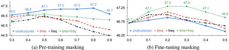We fine-tune Figure 4: Masking strategy . For pre-training, a higher ratio and unstructured masking (random) is preferred. For fine-tuning, a lower ratio and structured masking (time + frequency) is better. The y-axes are mAP on AS-2M and the x-axes are masking ratio. This ablation format follows [1]. <details> <summary>Image 4 Details</summary>  ### Visual Description ## Line Graphs: Pre-training and Fine-tuning Masking Performance ### Overview The image contains two line graphs comparing the performance of different masking strategies during pre-training and fine-tuning phases. Each graph shows four data series (unstructured, time, freq, time+freq) plotted against varying masking ratios. Performance is measured in percentage on the y-axis, while masking ratios are on the x-axis. ### Components/Axes **Graph (a): Pre-training Masking** - **X-axis**: Pre-training masking ratio (0.3 to 0.9) - **Y-axis**: Performance (%) (44.5 to 47.5) - **Legend**: - Blue squares: Unstructured - Red stars: Time - Black crosses: Freq - Green triangles: Time+freq **Graph (b): Fine-tuning Masking** - **X-axis**: Fine-tuning masking ratio (0.0 to 0.5) - **Y-axis**: Performance (%) (46.25 to 47.25) - **Legend**: Same as (a) ### Detailed Analysis **Graph (a) Trends**: 1. **Unstructured (blue)**: Starts at 46.6, peaks at 47.3 (0.7 masking), then declines to 46.7. 2. **Time (red)**: Starts at 46.6, peaks at 46.8 (0.4 masking), then declines to 45.5. 3. **Freq (black)**: Starts at 45.8, peaks at 46.5 (0.5 masking), then declines to 45.0. 4. **Time+freq (green)**: Starts at 46.3, peaks at 46.8 (0.4 masking), then declines to 46.3. **Graph (b) Trends**: 1. **Unstructured (blue)**: Starts at 46.7, peaks at 47.1 (0.1 masking), then declines to 46.9. 2. **Time (red)**: Starts at 46.7, peaks at 47.3 (0.2 masking), then declines to 46.6. 3. **Freq (black)**: Starts at 46.7, peaks at 47.1 (0.1 masking), then declines to 46.5. 4. **Time+freq (green)**: Starts at 46.7, peaks at 47.3 (0.2 masking), then declines to 46.9. ### Key Observations 1. **Pre-training Masking**: - Time+freq achieves the highest peak (47.3) at 0.7 masking. - Unstructured masking outperforms others initially but drops sharply after 0.7. - Freq masking shows the steepest decline post-peak. 2. **Fine-tuning Masking**: - Time+freq maintains the highest performance (47.3) at 0.2 masking. - All strategies show performance drops after their respective peaks. - Unstructured masking declines more sharply than others. ### Interpretation - **Optimal Masking Strategy**: Time+freq consistently outperforms other strategies in both phases, suggesting that combining temporal and frequency-based masking is most effective. - **Performance Peaks**: Both graphs show performance peaks at intermediate masking ratios (0.4–0.7 for pre-training, 0.1–0.2 for fine-tuning), indicating diminishing returns at higher masking ratios. - **Unstructured Masking**: While competitive in pre-training, its sharp decline in fine-tuning suggests it may overfit or lack adaptability during later stages. - **Anomalies**: Freq masking underperforms in pre-training but matches time+freq in fine-tuning, hinting at context-dependent efficacy. The data implies that hybrid masking strategies (time+freq) balance exploration and exploitation better than single-axis approaches, though further analysis is needed to explain the performance drops at higher masking ratios. </details> for 100 epochs, which aggregate to ∼ 10 full epochs of AudioSet-2M. The probability of sampling an instance is inversely proportional to the dataset-wise occurrences of its classes. Fine-tuning on 64 GPUs takes ∼ 12 hours. For the smaller balanced AudioSet-20K, we fine-tune on 4 GPUs for 60 epochs without weighted sampling. Please see Supplementary for the details on other datasets. ## 4.4 Ablations and Model Properties Masking Strategies in Pre-training and Fine-tuning. In Fig. 4, we compare different pre-training and fine-tuning masking strategies for Audio-MAE. First, in Fig. 4a we explore the pre-training masking ratio . We observe, similar as in MAE for images [1], that a high pre-training masking ratio (80% in our case) is optimal for audio spectrograms. This is due to the fact that both audio spectrograms and images are continuous signals with significant redundancy. Further, we find the unstructured random masking works the best for self-supervised pre-training over more structured masking ( e.g ., time + frequency). 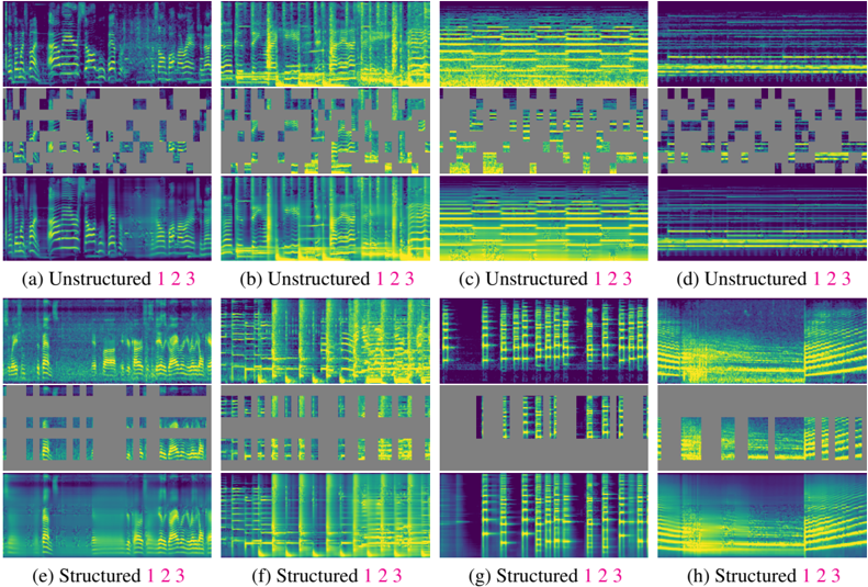Unlike MAE for images, there are clear performance differences among masking strategies when pre-training with audio spectrograms. Comparing Audio-MAE reconstructions between Fig. 6a to 6e and 6d to 6h, under the same masking ratio, we observe the unstructured random masking is comparably easier than structured masking ( i.e ., time and/or frequency) as the model can guess the missing component by extrapolating nearby context ( e.g ., formants in vowels and frictional sounds in consonants around). We also observe that for higher masking ratios, the structured masking alternatives drop in performance, presumably because the task becomes too difficult while random masking improves steadily up to 80%. This result show that designing a pretext task with proper hardness is important for effective self-supervised learning of audio representations. We therefore use random masking with ratio of 80% as our default for pre-training. Fig. 4b studies the effect of masking during the fine-tuning phase. We see that in this case, it is more beneficial to use structured masking: time + frequency performs better than time- or frequency-based masking, and these perform better than unstructured masking. Overall, we see that the optimal masking ratios are lower than for pre-training and we use 0.3 as our default in the fine-tuning phase. In general, we observe that for task-agnostic pre-training, unstructured masking with a higher ratio is preferred. While in task-specific fine-tuning, structured masking with lower ratios performs better. Impact of Patch Size and Stride. Wecompare the performance of Audio-MAE trained with different patch sizes and strides in Table 1a. A non-zero overlap ( i.e ., stride < patch size) between patches will increase the number of patches and quadratically increase computation in floating point operations (FLOPs), as reported in the table. Most prior works follow AST [10] to use overlapped patches (patch = 16 and stride = 10 ) to boost end task performance. As shown in Table 1a, we do not observe a performance improvement using overlapped patches for Audio-MAE (both 47.3 mAP), presumably because due to overlap, the patch embedding can leak information into the masked patches. The non-overlapped 16 × 16 patches achieve a good balance between computation and performance. By default, we use this setup in our experiments. Encoder. We investigate the design choices of encoder and decoder architectures in Audio-MAE. Table 1b shows the trade-off between encoder model size and performance. As expected, larger models achieve better performance, at a cost of computation and memory. The accuracy gain of ViT-L over ViT-B/S is more significant on the smaller and balanced AS-20K. For ViT-S, the performance Table 1: Ablation studies on AS-2M . The gray entries are the default Audio-MAE setup (ViT-B encoder, decoder with shifted local attention, pre-trained for 32 epochs). Table format follows [1]. | Patch size, stride Seq shape FLOPs mAP | Backbone #Params AS-20K AS-2M | Patch size, stride Seq shape FLOPs mAP | Patch size, stride Seq shape FLOPs mAP | Patch size, stride Seq shape FLOPs mAP | Patch size, stride Seq shape FLOPs mAP | Patch size, stride Seq shape FLOPs mAP | |------------------------------------------|---------------------------------|------------------------------------------|------------------------------------------|------------------------------------------|------------------------------------------|------------------------------------------| gap to ViT-B can be significantly closed (5.0 → 2.3 mAP) when fine-tuning with more in-domain data (AS-20K → AS-2M). 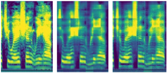Decoder. Table 1c compares decoder attention types in Audio-MAE. Note that decoders are discarded after pretraining and only the equal-sized ViT-B encoders are fine-tuned for the end task. Our results show that local attention with shifted window achieves the best performance. Combining local and global attention ( i.e ., hybrid attention, Hwin) also improves vanilla global self-attention. Fig. 5 shows the qualitative reconstruction comparison. In the spectrogram of vowels, the decoder with local attention reconstructs better harmonics and recovers more context in the spectrogram. Similar phenomena are observed in the frictional sound in the middle consonant. Ground-Truth w/ global attention w/ local attention <details> <summary>Image 5 Details</summary>  ### Visual Description ## Heatmaps: Comparative Analysis of Three Panels ### Overview The image displays three adjacent heatmaps with color gradients ranging from dark blue (low values) to bright yellow (high values). No textual labels, legends, or axis markers are visible. The panels appear to represent spatial or temporal distributions of an unspecified metric. ### Components/Axes - **Structure**: - Each heatmap is divided into a grid-like pattern with vertical and horizontal bands. - Color intensity varies across the grid, suggesting a scalar value mapped to a color scale (e.g., 0–100% or categorical intensity). - **Spatial Arrangement**: - **Panel 1 (Left)**: Dominated by vertical yellow streaks on the left and right edges, with a central region of alternating blue and yellow bands. - **Panel 2 (Center)**: Features a checkerboard-like pattern with alternating blue and yellow squares, interrupted by vertical yellow bands near the center. - **Panel 3 (Right)**: Shows a more uniform distribution of yellow bands concentrated in the upper and lower regions, with a central blue-dominated area. ### Detailed Analysis - **Color Distribution**: - **Panel 1**: Yellow regions occupy ~30% of the total area, concentrated in vertical bands. Blue regions dominate (~70%), with wavy horizontal gradients. - **Panel 2**: Yellow and blue regions are nearly equal (~50% each), with a grid-like alternation. Vertical yellow bands occupy ~20% of the width. - **Panel 3**: Yellow regions occupy ~40% of the area, primarily in the upper and lower thirds. Blue regions dominate the central ~60%. - **Notable Patterns**: - Panel 1 exhibits wave-like horizontal gradients, suggesting a sinusoidal or oscillatory trend. - Panel 2’s checkerboard pattern implies a binary or alternating categorical distribution. - Panel 3’s asymmetry (yellow concentrated at top/bottom) may indicate boundary effects or directional bias. ### Key Observations 1. **Panel 1**: High-intensity (yellow) regions are localized and vertical, contrasting with the diffuse blue background. 2. **Panel 2**: Regular alternation of colors suggests a structured, possibly binary system (e.g., on/off states). 3. **Panel 3**: Asymmetrical yellow distribution implies a non-uniform process, such as directional flow or edge dominance. ### Interpretation The heatmaps likely represent variations in a physical, biological, or computational system. The absence of legends or labels prevents precise quantification, but the following inferences can be made: - **Panel 1** may depict a system with localized peaks (e.g., signal strength, temperature) against a baseline. - **Panel 2** could represent a binary classification or alternating process (e.g., on/off cycles, categorical states). - **Panel 3** might illustrate a directional phenomenon (e.g., fluid flow, wave propagation) with boundary-driven intensity. **Critical Limitation**: Without axis labels, legends, or contextual metadata, the exact nature of the data (e.g., units, categories) remains speculative. The analysis is constrained to visual pattern recognition. </details> Figure 5: Decoder reconstruction comparison. Table 1d ablates the impact of decoder depth on mAP. A deeper 16-layer decoder achieves better performance against its shallower variants. Note that our decoder uses local window attention by default where only a fraction of tokens (4 × 4 local windows vs. 64 × 8 with global attention) are attended. For global attention we find 8-layer decoders to perform better than 16-layer. Table 1e compares decoder width (embedding dimension). A 512-dimension decoder achieves a good trade-off between computation and performance as a wider one is not better. Pre-training Data and Setup. Table 1f summarizes the impact of pre-training dataset size. Overall the model performance is monotonically increasing when using more data for pre-training. Comparing the performance of using 1% well-annotated AS-20K balanced data to using randomly sampled 20K unbalanced data for pre-training, the similar mAPs (39.4 vs 39.6) suggest that the distribution of data classes (balanced vs. unbalanced) is less important for pre-training. Meanwhile, as shown in Table 1g, training for longer is beneficial yet the performance saturates after the 24th epoch. Out-of-domain Pre-training on ImageNet. Initializing audio models from ImageNet pre-trained weights has become popular for audio classification. However, as there are significant discrepancies between image and audio modalities, it is questionable if out-of-domain pre-training benefits audio representation learning. In Table 1h we design 3 scenarios to investigate this for Audio-MAE: (1) Table 2: Comparison with other state-of-the-art models on audio and speech classification tasks. Metrics are mAP for AS and accuracy (%) for ESC/SPC/SID. For pre-training (PT) dataset, AS:AudioSet, LS:LibriSpeech, and IN:ImageNet. † : Fine-tuning results with additional supervised training on AS-2M. We gray-out models pre-trained with external non-audio datasets ( e.g ., ImageNet). Best single models in AS-2M are compared (no ensembles). * : linear evaluation results from [53]. | Model | Backbone | PT-Data | AS-20K | AS-2M | ESC-50 | SPC-2 | SPC-1 | SID | |----------------------------------------|----------------------------------------|----------------------------------------|----------------------------------------|----------------------------------------|----------------------------------------|----------------------------------------|----------------------------------------|----------------------------------------| | No pre-training | No pre-training | No pre-training | No pre-training | No pre-training | No pre-training | No pre-training | No pre-training | No pre-training | | ERANN [58] | CNN | - | - | 45.0 | 89.2 | - | - | - | | PANN [59] | CNN | - | 27.8 | 43.1 | 83.3 | 61.8 | - | - | | In-domain self-supervised pre-training | In-domain self-supervised pre-training | In-domain self-supervised pre-training | In-domain self-supervised pre-training | In-domain self-supervised pre-training | In-domain self-supervised pre-training | In-domain self-supervised pre-training | In-domain self-supervised pre-training | In-domain self-supervised pre-training | | wav2vec 2.0 [33] | Transformer | LS | - | - | - | - | 96.2 * | 75.2 * | | HuBERT [35] | Transformer | LS | - | - | - | - | 96.3 * | 81.4 * | | Conformer [37] | Conformer | AS | - | 41.1 | 88.0 | - | - | - | | SS-AST [18] | ViT-B | AS+LS | 31.0 | - | 88.8 | 98.0 | 96.0 | 64.3 | | Concurrent MAE-based works | Concurrent MAE-based works | Concurrent MAE-based works | Concurrent MAE-based works | Concurrent MAE-based works | Concurrent MAE-based works | Concurrent MAE-based works | Concurrent MAE-based works | Concurrent MAE-based works | | MaskSpec [43] | ViT-B | AS | 32.3 | 47.1 | 89.6 | 97.7 | - | - | | MAE-AST [38] | ViT-B | AS+LS | 30.6 | - | 90.0 | 97.9 | 95.8 | 63.3 | | Audio-MAE (global) | ViT-B | AS | 36.6 ± . 11 | 46.8 ± . 06 | 93.6 ± . 11 | 98.3 ± . 06 | 97.6 ± . 06 | 94.1 ± . 06 | | Audio-MAE (local) | ViT-B | AS | 37.0 ± . 11 | 47.3 ± . 11 | 94.1 ± . 10 | 98.3 ± . 06 | 96.9 ± . 00 | 94.8 ± . 11 | | Out-of-domain supervised pre-training | Out-of-domain supervised pre-training | Out-of-domain supervised pre-training | Out-of-domain supervised pre-training | Out-of-domain supervised pre-training | Out-of-domain supervised pre-training | Out-of-domain supervised pre-training | Out-of-domain supervised pre-training | Out-of-domain supervised pre-training | | PSLA [30] | EffNet [60] | IN | 31.9 | 44.4 | - | 96.3 | - | - | | AST [10] | DeiT-B | IN | 34.7 | 45.9 | 88.7 | 98.1 | 95.5 | 41.1 | | MBT [11] | ViT-B | IN-21K | 31.3 | 44.3 | - | - | - | - | | HTS-AT [29] | Swin-B | IN | - | 47.1 | 97.0 † | 98.0 | - | - | | PaSST [28] | DeiT-B | IN | - | 47.1 | 96.8 † | - | - | - | Audio-only pre-training (AS-SSL) from scratch. We consider this the ideal schema for learning audio representations as it is a simple and clean setup that prevents uncontrollable bias transfer from other modalities. (2) Directly using self-supervised ImageNet MAE models (IN-SSL) and its fine-tuned variant (IN-SL). (3) Audio-MAE self-supervised pre-training on top of these ImageNet weights. The results show that (1) from-scratch audio-only pre-training is the best. For scenarios (2) and (3), we observe that ImageNet pre-training alone (2) is not sufficient (especially when the downstream data is smaller, AS-20K), and, in self-supervised pre-training on AudioSet, ImageNet initialization (3) does not help but degrades accuracy. Also in (3), supervised ImageNet pre-training (IN-SL) seems harmful. Consequently, the result suggests that out-of-domain pre-training ( i.e ., ImageNet) is not helpful for Audio-MAE, possibly due to domain shift. ## 4.5 Comparison with the State-of-the-art Table 2 compares Audio-MAE (with 3-run error bars) to prior state-of-the-art. We categorize the comparison into 3 groups. For fair comparison, our main benchmark is the models in the middle group with self-supervised pre-training on in-domain (audio) datasets (AudioSet and LibriSpeech). For reference we also list other models without pre-training (the top group) and other models with supervised pre-training on out-of-domain ImageNet (the bottom group), where the latter contains previous best systems on the datasets. Pre-trained on AudioSet, Audio-MAE achieves the best performance across all tasks compared to other models with in-domain self-supervised pre-training. On AudioSet-20K, its 37.1 mAP significantly outperforms all other approaches including concurrent works and other models with outof-domain pre-training. On AudioSet-2M and ESC-50, our method also outperforms Conformer [37] and SS-AST [18]. Notably, unlike SS-AST and concurrent MAE-AST [38], which trained with additional 1,000 hours of speech in Librispeech, we use only AudioSet for pre-training. In the bottom group of Table 2, Audio-MAE also outperforms previous state-of-the-art models with ImageNet supervised pre-training. Note that the proposed Audio-MAE does not rely on any out-ofdomain data and labels, nor using knowledge distillation ( e.g ., DeiT) from additional CNN-based models. Also, compared to HTS-AT [29] and PaSST [28], Audio-MAE is trained with audio under 16K sampling rate. As experimented in [59], there could be up to 0.4 potential mAP improvement for Audio-MAE if audio with 32K sampling rate are available. Figure 6: Spectrogram reconstruction visualizations on the AudioSet eval set . Column-wise type: speech, music, event, others. Masking type: (a-d) unstructured (random); (e-h) structured (time + frequency). Masking Ratio: 70%. In each group, we show the original spectrogram (1, top), masked input (2, middle), and MAE output (3, bottom). The spectrogram size is 1024 × 128; patch size is 16 × 16. Each sample has 64 × 8=512 patches with 154 (70% masked) patches being visible to Audio-MAE. Please click (1 2 3) for audible .wav s. More audible examples are in Supplementary. <details> <summary>Image 6 Details</summary>  ### Visual Description ## Heatmap Visualization: Structured vs. Unstructured Configurations ### Overview The image presents eight heatmaps (labeled a-h) comparing "Structured" and "Unstructured" configurations across three categories (1, 2, 3). Each panel displays a 3x3 grid of color-coded values, with variations in intensity and distribution. The heatmaps use a blue-to-yellow gradient, likely representing magnitude or frequency, though no explicit legend is provided. ### Components/Axes - **Rows**: - Top row: "Unstructured 1 2 3" (panels a-d) - Middle row: "Structured 1 2 3" (panels e-h) - **Columns**: - Left column: "Unstructured 1 2 3" (panels a, e) - Right column: "Structured 1 2 3" (panels b, f, g, h) - **Heatmap Labels**: - Panels a-d: "Unstructured 1 2 3" - Panels e-h: "Structured 1 2 3" - **Color Gradient**: Blue (low values) to Yellow (high values), no explicit legend. ### Detailed Analysis #### Unstructured Configurations (a-d) - **Panel a**: Vertical stripes dominate, with alternating blue and yellow bands. - **Panel b**: Horizontal stripes with sparse yellow blocks. - **Panel c**: Scattered yellow blocks on a blue background, suggesting localized high values. - **Panel d**: Uniform blue with faint yellow streaks, indicating minimal variation. #### Structured Configurations (e-h) - **Panel e**: Vertical stripes with consistent spacing, resembling a grid. - **Panel f**: Horizontal stripes with dense yellow blocks, suggesting higher values. - **Panel g**: Vertical stripes with sharp transitions, indicating abrupt changes. - **Panel h**: Grid-like pattern with alternating blue and yellow blocks, showing structured regularity. ### Key Observations 1. **Structured vs. Unstructured**: - Structured configurations (e-h) exhibit more organized patterns (stripes, grids) compared to unstructured (a-d), which show irregular or sparse distributions. - Structured panels (f, h) have higher yellow intensity, implying greater magnitude or frequency. 2. **Color Trends**: - Yellow regions (high values) are more concentrated in structured configurations, particularly in panels f and h. - Unstructured panels (a, c) show fragmented or isolated yellow areas. 3. **Missing Legend**: - The absence of a legend prevents precise interpretation of color values. However, the blue-to-yellow gradient likely represents a scale from low to high. ### Interpretation The visual data suggests that structured configurations produce more consistent and organized patterns, potentially indicating improved performance or stability. Unstructured configurations exhibit variability, with some panels (e.g., c) showing localized high values but no clear trend. The lack of a legend limits quantitative analysis, but the spatial distribution of colors implies that structured approaches may yield more predictable outcomes. ### Notes - No numerical data or explicit axis titles are present. - All text is in English; no other languages are detected. - The heatmaps lack a legend, so color interpretation relies on visual inference. </details> For the speech tasks (SPC-1, SPC-2, and SID), Audio-MAE outperforms other models without pre-training (ERANN [58], PANN [59]), supervised (AST) and self-supervised models (SS-AST, MAE-AST). We further list other works (marked with * ) to include the latest results introduced in the SUPERB [53] benchmark. But note that these results are not strictly comparable since SUPERB employs linear evaluation where the underlying pre-trained models are not end-to-end fine-tuned. In summary, with audio-only from-scratch pre-training on AudioSet, our Audio-MAE performs well for both the audio and speech classification tasks. ## 4.6 Visualization and Audible Examples by Audio-MAE Decoder For better visualization, we follow MAE [1] to use MSE over non-normalized spectrograms as the selfsupervised objective. We use ViT-L as the Audio-MAE encoder for visualization. Fig. 6 illustrates the reconstruction results sampled from the AudioSet-2M eval set. We further reconstruct .wav s using the Griffin-Lim [61] algorithm, audible under the anonymous links (accessible in respective 1 2 3). As can be seen and heard, for various masking strategies and different sounds, our Audio-MAE generates reasonable reconstruction. It works well for noisy event sounds ( e.g ., the reconstructed siren in Fig. 6c-3), as well as speech and music ( e.g ., the reconstructed singing in Fig. 6b-3). Notably, unlike visual contents that are typically scale/translation/position invariant [19], absolute positions and arrangement of spectrogram components are critical for humans to understand sound [62]. For example, shifting a pitch will make an audio sounds completely different. Also, phoneme sequences in time are important cues for speech understanding. Consequently, unstructured masking produces better aligned outputs that are closer to the ground-truth (top row in each subfigure) as the model can make better predictions based on nearby spectrogram patches; while structured masking is harder (less accurate or with words missing), especially when masking is performed over the time axis. A failure example (missing words) is the reconstructed speech in Fig. 6e-3. ## 5 Conclusion We have explored a simple extension of MAE [1] to audio data. Our Audio-MAE learns to reconstruct masked spectrogram patches from audio recordings and achieves state-of-the-art performance on six audio and speech classification tasks. We have drawn four interesting observations: First, a simple MAE approach works surprisingly well for audio spectrograms. Second, we find that it is possible to learn stronger representations with local self-attention in the decoder. Third, we show that masking can be applied to both pre-training and fine-tuning, improving accuracy and reducing training computation. The optimal strategy depends on the nature of the data (audio, image, etc .) and the learning type (self-/supervised). Fourth, the best performance can be achieved by pre-training and fine-tuning under the same modality, without reliance on cross-modality transfer learning. In future work, we aim to explore multimodal self-supervised learning with a joint audio-visual MAE approach as these domains share natural correspondences in video data. Acknowledgements. Wethank Kaiming He and Luke Zettlemoyer for their feedback and discussions. ## References - [1] K. He, X. Chen, S. Xie, Y. Li, P. Dollár, and R. Girshick, 'Masked autoencoders are scalable vision learners,' arXiv preprint arXiv:2111.06377 , 2021. - [2] A. Vaswani, N. Shazeer, N. Parmar, J. Uszkoreit, L. Jones, A. N. Gomez, L. Kaiser, and I. Polosukhin, 'Attention is all you need,' in Proceedings of the 31st International Conference on Neural Information Processing Systems , ser. NIPS'17. USA: Curran Associates Inc., 2017, pp. 6000-6010. - [3] J. Devlin, M. Chang, K. Lee, and K. Toutanova, 'BERT: pre-training of deep bidirectional transformers for language understanding,' in Proceedings of the 2019 Conference of the North American Chapter of the Association for Computational Linguistics: Human Language Technologies, NAACL-HLT 2019, Minneapolis, MN, USA, June 2-7, 2019, Volume 1 (Long and Short Papers) . Association for Computational Linguistics, 2019, pp. 4171-4186. - [4] T. B. Brown, B. Mann, N. Ryder, M. Subbiah, J. Kaplan, P. Dhariwal, A. Neelakantan, P. Shyam, G. Sastry, A. Askell, S. Agarwal, A. Herbert-Voss, G. Krueger, T. Henighan, R. Child, A. Ramesh, D. M. Ziegler, J. Wu, C. Winter, C. Hesse, M. Chen, E. Sigler, M. Litwin, S. Gray, B. Chess, J. Clark, C. Berner, S. McCandlish, A. Radford, I. Sutskever, and D. Amodei, 'Language models are few-shot learners,' in Advances in Neural Information Processing Systems 33: Annual Conference on Neural Information Processing Systems 2020, NeurIPS 2020, December 6-12, 2020, virtual , 2020. - [5] Y. Liu, M. Ott, N. Goyal, J. Du, M. Joshi, D. Chen, O. Levy, M. Lewis, L. Zettlemoyer, and V. Stoyanov, 'Roberta: A robustly optimized BERT pretraining approach,' CoRR , vol. abs/1907.11692, 2019. - [6] K. He, H. Fan, Y. Wu, S. Xie, and R. B. Girshick, 'Momentum contrast for unsupervised visual representation learning,' in 2020 IEEE/CVF Conference on Computer Vision and Pattern Recognition, CVPR 2020, Seattle, WA, USA, June 13-19, 2020 . Computer Vision Foundation / IEEE, 2020, pp. 9726-9735. - [7] X. Chen, S. Xie, and K. He, 'An empirical study of training self-supervised vision transformers,' in 2021 IEEE/CVF International Conference on Computer Vision, ICCV 2021, Montreal, QC, Canada, October 10-17, 2021 . IEEE, 2021, pp. 9620-9629. - [8] R. Paulus, C. Xiong, and R. Socher, 'A deep reinforced model for abstractive summarization,' arXiv , vol. abs/1705.04304, 2017. - [9] A. Dosovitskiy, L. Beyer, A. Kolesnikov, D. Weissenborn, X. Zhai, T. Unterthiner, M. Dehghani, M. Minderer, G. Heigold, S. Gelly et al. , 'An image is worth 16x16 words: Transformers for image recognition at scale,' arXiv preprint arXiv:2010.11929 , 2020. - [10] Y. Gong, Y. Chung, and J. R. Glass, 'AST: audio spectrogram transformer,' in Interspeech 2021, 22nd Annual Conference of the International Speech Communication Association, Brno, Czechia, 30 August - 3 September 2021 . ISCA, 2021, pp. 571-575. - [11] A. Nagrani, S. Yang, A. Arnab, A. Jansen, C. Schmid, and C. Sun, 'Attention bottlenecks for multimodal fusion,' in Advances in Neural Information Processing Systems 34: Annual - Conference on Neural Information Processing Systems 2021, NeurIPS 2021, December 6-14, 2021, virtual , 2021, pp. 14 200-14 213. - [12] J. F. Gemmeke, D. P. Ellis, D. Freedman, A. Jansen, W. Lawrence, R. C. Moore, M. Plakal, and M. Ritter, 'Audio set: An ontology and human-labeled dataset for audio events,' in 2017 IEEE International Conference on Acoustics, Speech and Signal Processing (ICASSP) . IEEE, 2017, pp. 776-780. - [13] K. J. Piczak, 'ESC: Dataset for Environmental Sound Classification,' in Proceedings of the 23rd Annual ACM Conference on Multimedia . ACM Press, 2015, pp. 1015-1018. - [14] H. Touvron, M. Cord, M. Douze, F. Massa, A. Sablayrolles, and H. Jégou, 'Training dataefficient image transformers & distillation through attention,' in International Conference on Machine Learning . PMLR, 2021, pp. 10 347-10 357. - [15] J. Carreira and A. Zisserman, 'Quo vadis, action recognition? A new model and the kinetics dataset,' in 2017 IEEE Conference on Computer Vision and Pattern Recognition, CVPR 2017, Honolulu, HI, USA, July 21-26, 2017 . IEEE Computer Society, 2017, pp. 4724-4733. - [16] C. Feichtenhofer, A. Pinz, and R. P. Wildes, 'Spatiotemporal residual networks for video action recognition,' in NIPS , 2016. - [17] H. Bao, L. Dong, and F. Wei, 'Beit: BERT pre-training of image transformers,' CoRR , vol. abs/2106.08254, 2021. - [18] Y. Gong, C.-I. Lai, Y.-A. Chung, and J. R. Glass, 'Ssast: Self-supervised audio spectrogram transformer,' ArXiv , vol. abs/2110.09784, 2021. - [19] Z. Liu, Y. Lin, Y. Cao, H. Hu, Y. Wei, Z. Zhang, S. Lin, and B. Guo, 'Swin transformer: Hierarchical vision transformer using shifted windows,' in 2021 IEEE/CVF International Conference on Computer Vision, ICCV 2021, Montreal, QC, Canada, October 10-17, 2021 . IEEE, 2021, pp. 9992-10 002. - [20] C. Wei, H. Fan, S. Xie, C. Wu, A. L. Yuille, and C. Feichtenhofer, 'Masked feature prediction for self-supervised visual pre-training,' CoRR , vol. abs/2112.09133, 2021. - [21] P. Vincent, H. Larochelle, Y. Bengio, and P. Manzagol, 'Extracting and composing robust features with denoising autoencoders,' in Machine Learning, Proceedings of the Twenty-Fifth International Conference (ICML 2008), Helsinki, Finland, June 5-9, 2008 , ser. ACM International Conference Proceeding Series, vol. 307. ACM, 2008, pp. 1096-1103. - [22] P. Vincent, H. Larochelle, I. Lajoie, Y. Bengio, and P. Manzagol, 'Stacked denoising autoencoders: Learning useful representations in a deep network with a local denoising criterion,' J. Mach. Learn. Res. , vol. 11, pp. 3371-3408, 2010. - [23] D. Pathak, P. Krähenbühl, J. Donahue, T. Darrell, and A. A. Efros, 'Context encoders: Feature learning by inpainting,' in 2016 IEEE Conference on Computer Vision and Pattern Recognition, CVPR 2016, Las Vegas, NV, USA, June 27-30, 2016 . IEEE Computer Society, 2016, pp. 2536-2544. - [24] M. Chen, A. Radford, R. Child, J. Wu, H. Jun, D. Luan, and I. Sutskever, 'Generative pretraining from pixels,' in Proceedings of the 37th International Conference on Machine Learning, ICML 2020, 13-18 July 2020, Virtual Event , ser. Proceedings of Machine Learning Research, vol. 119. PMLR, 2020, pp. 1691-1703. - [25] A. Ramesh, M. Pavlov, G. Goh, S. Gray, C. Voss, A. Radford, M. Chen, and I. Sutskever, 'Zero-shot text-to-image generation,' in Proceedings of the 38th International Conference on Machine Learning, ICML 2021, 18-24 July 2021, Virtual Event , ser. Proceedings of Machine Learning Research, vol. 139. PMLR, 2021, pp. 8821-8831. - [26] N. Dalal and B. Triggs, 'Histograms of oriented gradients for human detection,' in 2005 IEEE Computer Society Conference on Computer Vision and Pattern Recognition (CVPR 2005), 20-26 June 2005, San Diego, CA, USA . IEEE Computer Society, 2005, pp. 886-893. - [27] K. He, X. Zhang, S. Ren, and J. Sun, 'Deep residual learning for image recognition,' 2016 IEEE Conference on Computer Vision and Pattern Recognition (CVPR) , pp. 770-778, 2015. - [28] K. Koutini, J. Schlüter, H. Eghbal-zadeh, and G. Widmer, 'Efficient training of audio transformers with patchout,' CoRR , vol. abs/2110.05069, 2021. - [29] K. Chen, X. Du, B. Zhu, Z. Ma, T. Berg-Kirkpatrick, and S. Dubnov, 'Hts-at: A hierarchical token-semantic audio transformer for sound classification and detection,' arXiv preprint arXiv:2202.00874 , 2022. - [30] Y. Gong, Y. Chung, and J. Glass, 'Psla: Improving audio tagging with pretraining, sampling, labeling, and aggregation,' IEEE/ACM Transactions on Audio, Speech, and Language Processing , 2021. - [31] Y. Gong, S. Khurana, A. Rouditchenko, and J. Glass, 'Cmkd: Cnn/transformer-based cross-model knowledge distillation for audio classification,' 2022. - [32] S. Schneider, A. Baevski, R. Collobert, and M. Auli, 'wav2vec: Unsupervised pre-training for speech recognition,' in Interspeech 2019, 20th Annual Conference of the International Speech Communication Association, Graz, Austria, 15-19 September 2019 . ISCA, 2019, pp. 3465-3469. - [33] A. Baevski, Y. Zhou, A. Mohamed, and M. Auli, 'wav2vec 2.0: A framework for self-supervised learning of speech representations,' in Advances in Neural Information Processing Systems 33: Annual Conference on Neural Information Processing Systems 2020, NeurIPS 2020, December 6-12, 2020, virtual , 2020. - [34] A. Baevski, W. Hsu, Q. Xu, A. Babu, J. Gu, and M. Auli, 'data2vec: A general framework for self-supervised learning in speech, vision and language,' CoRR , vol. abs/2202.03555, 2022. - [35] W.-N. Hsu, B. Bolte, Y.-H. H. Tsai, K. Lakhotia, R. Salakhutdinov, and A. Mohamed, 'Hubert: Self-supervised speech representation learning by masked prediction of hidden units,' IEEE/ACM Transactions on Audio, Speech, and Language Processing , vol. 29, pp. 3451-3460, 2021. - [36] B. Shi, W. Hsu, and A. Mohamed, 'Robust self-supervised audio-visual speech recognition,' CoRR , vol. abs/2201.01763, 2022. - [37] S. Srivastava, Y . Wang, A. Tjandra, A. Kumar, C. Liu, K. Singh, and Y. Saraf, 'Conformer-based self-supervised learning for non-speech audio tasks,' arXiv preprint arXiv:2110.07313 , 2021. - [38] A. Baade, P. Peng, and D. Harwath, 'Mae-ast: Masked autoencoding audio spectrogram transformer,' arXiv preprint arXiv:2203.16691 , 2022. - [39] A. van den Oord, Y. Li, and O. Vinyals, 'Representation learning with contrastive predictive coding,' CoRR , vol. abs/1807.03748, 2018. - [40] R. Arandjelovic and A. Zisserman, 'Objects that sound,' in Computer Vision - ECCV 2018 15th European Conference, Munich, Germany, September 8-14, 2018, Proceedings, Part I , ser. Lecture Notes in Computer Science, vol. 11205. Springer, 2018, pp. 451-466. - [41] M. Patrick, P. Huang, I. Misra, F. Metze, A. Vedaldi, Y. M. Asano, and J. F. Henriques, 'Space-time crop & attend: Improving cross-modal video representation learning,' in 2021 IEEE/CVF International Conference on Computer Vision, ICCV 2021, Montreal, QC, Canada, October 10-17, 2021 . IEEE, 2021, pp. 10 540-10 552. - [42] A. T. Liu, S. Yang, P. Chi, P. Hsu, and H. Lee, 'Mockingjay: Unsupervised speech representation learning with deep bidirectional transformer encoders,' in 2020 IEEE International Conference on Acoustics, Speech and Signal Processing, ICASSP 2020, Barcelona, Spain, May 4-8, 2020 . IEEE, 2020, pp. 6419-6423. - [43] D. Chong, H. Wang, P. Zhou, and Q. Zeng, 'Masked spectrogram prediction for self-supervised audio pre-training,' 2022. - [44] D. Niizumi, D. Takeuchi, Y. Ohishi, N. Harada, and K. Kashino, 'Masked spectrogram modeling using masked autoencoders for learning general-purpose audio representation,' arXiv:2204.12260 , 2022. - [45] Y. Li, C.-Y. Wu, H. Fan, K. Mangalam, B. Xiong, J. Malik, and C. Feichtenhofer, 'Mvitv2: Improved multiscale vision transformers for classification and detection,' in CVPR , 2022. - [46] A. van den Oord, Y. Li, and O. Vinyals, 'Representation learning with contrastive predictive coding,' CoRR , vol. abs/1807.03748, 2018. - [47] A. Baevski, M. Auli, and A. Mohamed, 'Effectiveness of self-supervised pre-training for speech recognition,' CoRR , vol. abs/1911.03912, 2019. - [48] D. S. Park, W. Chan, Y. Zhang, C.-C. Chiu, B. Zoph, E. D. Cubuk, and Q. V. Le, 'Specaugment: A simple data augmentation method for automatic speech recognition,' ArXiv , vol. abs/1904.08779, 2019. - [49] J. B. Li, S. Qu, P. Huang, and F. Metze, 'Audiotagging done right: 2nd comparison of deep learning methods for environmental sound classification,' CoRR , vol. abs/2203.13448, 2022. - [50] S. Hershey, S. Chaudhuri, D. P. W. Ellis, J. F. Gemmeke, A. Jansen, C. Moore, M. Plakal, D. Platt, R. A. Saurous, B. Seybold, M. Slaney, R. Weiss, and K. Wilson, 'Cnn architectures for large-scale audio classification,' in International Conference on Acoustics, Speech and Signal Processing (ICASSP) , 2017. - [51] S. Hershey, D. P. Ellis, E. Fonseca, A. Jansen, C. Liu, R. C. Moore, and M. Plakal, 'The benefit of temporally-strong labels in audio event classification,' in ICASSP 2021-2021 IEEE International Conference on Acoustics, Speech and Signal Processing (ICASSP) . IEEE, 2021, pp. 366-370. - [52] P. Warden, 'Speech Commands: A Dataset for Limited-Vocabulary Speech Recognition,' ArXiv e-prints , Apr. 2018. - [53] S. wen Yang, P.-H. Chi, Y.-S. Chuang, C.-I. J. Lai, K. Lakhotia, Y. Y. Lin, A. T. Liu, J. Shi, X. Chang, G.-T. Lin, T.-H. Huang, W.-C. Tseng, K. tik Lee, D.-R. Liu, Z. Huang, S. Dong, S.-W. Li, S. Watanabe, A. Mohamed, and H. yi Lee, 'SUPERB: Speech Processing Universal PERformance Benchmark,' in Proc. Interspeech 2021 , 2021, pp. 1194-1198. - [54] A. Nagrani, J. S. Chung, W. Xie, and A. Zisserman, 'Voxceleb: Large-scale speaker verification in the wild,' Comput. Speech Lang. , vol. 60, 2020. - [55] D. Povey, A. Ghoshal, G. Boulianne, L. Burget, O. Glembek, N. Goel, M. Hannemann, P. Motlicek, Y. Qian, P. Schwarz et al. , 'The kaldi speech recognition toolkit,' in IEEE 2011 workshop on automatic speech recognition and understanding , no. CONF. IEEE Signal Processing Society, 2011. - [56] S. Yun, D. Han, S. Chun, S. J. Oh, Y. Yoo, and J. Choe, 'Cutmix: Regularization strategy to train strong classifiers with localizable features,' in 2019 IEEE/CVF International Conference on Computer Vision, ICCV 2019, Seoul, Korea (South), October 27 - November 2, 2019 . IEEE, 2019, pp. 6022-6031. - [57] H. Zhang, M. Cissé, Y. N. Dauphin, and D. Lopez-Paz, 'mixup: Beyond empirical risk minimization,' in 6th International Conference on Learning Representations, ICLR 2018, Vancouver, BC, Canada, April 30 - May 3, 2018, Conference Track Proceedings . OpenReview.net, 2018. - [58] S. Verbitskiy, V. Berikov, and V. Vyshegorodtsev, 'Eranns: Efficient residual audio neural networks for audio pattern recognition,' arXiv preprint arXiv:2106.01621 , 2021. - [59] Q. Kong, Y. Cao, T. Iqbal, Y. Wang, W. Wang, and M. D. Plumbley, 'Panns: Large-scale pretrained audio neural networks for audio pattern recognition,' IEEE ACM Trans. Audio Speech Lang. Process. , vol. 28, pp. 2880-2894, 2020. - [60] M. Tan and Q. V. Le, 'Efficientnet: Rethinking model scaling for convolutional neural networks,' in Proceedings of the 36th International Conference on Machine Learning, ICML 2019, 9-15 June 2019, Long Beach, California, USA , ser. Proceedings of Machine Learning Research, vol. 97. PMLR, 2019, pp. 6105-6114. - [61] D. Griffin and J. Lim, 'Signal estimation from modified short-time fourier transform,' IEEE Transactions on Acoustics, Speech, and Signal Processing , vol. 32, no. 2, pp. 236-243, 1984. - [62] Y. Suzuki and H. Takeshima, 'Equal-loudness-level contours for pure tones,' The Journal of the Acoustical Society of America , vol. 116, no. 2, pp. 918-933, 2004. - [63] I. Loshchilov and F. Hutter, 'Decoupled weight decay regularization,' in 7th International Conference on Learning Representations, ICLR 2019, New Orleans, LA, USA, May 6-9, 2019 . OpenReview.net, 2019. - [64] --, 'SGDR: stochastic gradient descent with warm restarts,' in 5th International Conference on Learning Representations, ICLR 2017, Toulon, France, April 24-26, 2017, Conference Track Proceedings . OpenReview.net, 2017. - [65] G. Huang, Y. Sun, Z. Liu, D. Sedra, and K. Q. Weinberger, 'Deep networks with stochastic depth,' in Computer Vision - ECCV 2016 - 14th European Conference, Amsterdam, The Netherlands, October 11-14, 2016, Proceedings, Part IV , ser. Lecture Notes in Computer Science, vol. 9908. Springer, 2016, pp. 646-661. - [66] N. Srivastava, G. E. Hinton, A. Krizhevsky, I. Sutskever, and R. Salakhutdinov, 'Dropout: a simple way to prevent neural networks from overfitting,' J. Mach. Learn. Res. , vol. 15, no. 1, pp. 1929-1958, 2014. - [67] R. Müller, S. Kornblith, and G. E. Hinton, 'When does label smoothing help?' in Advances in Neural Information Processing Systems 32: Annual Conference on Neural Information Processing Systems 2019, NeurIPS 2019, December 8-14, 2019, Vancouver, BC, Canada , 2019, pp. 4696-4705. - [68] B. Lee and J. Chang, 'Packet loss concealment based on deep neural networks for digital speech transmission,' IEEE ACM Trans. Audio Speech Lang. Process. , vol. 24, no. 2, pp. 378-387, 2016. - [69] J. Lin, Y. Wang, K. Kalgaonkar, G. Keren, D. Zhang, and C. Fuegen, 'A time-domain convolutional recurrent network for packet loss concealment,' in ICASSP 2021 - 2021 IEEE International Conference on Acoustics, Speech and Signal Processing (ICASSP) , 2021, pp. 7148-7152. - [70] Y. Chang, K. Lee, P. Wu, H. Lee, and W. H. Hsu, 'Deep long audio inpainting,' CoRR , vol. abs/1911.06476, 2019. - [71] A. Marafioti, N. Perraudin, N. Holighaus, and P. Majdak, 'A context encoder for audio inpainting,' IEEE ACM Trans. Audio Speech Lang. Process. , vol. 27, no. 12, pp. 2362-2372, 2019. - [72] B. Liu, J. Tao, Z. Wen, Y. Li, and D. Bukhari, 'A novel method of artificial bandwidth extension using deep architecture,' in INTERSPEECH 2015, 16th Annual Conference of the International Speech Communication Association, Dresden, Germany, September 6-10, 2015 . ISCA, 2015, pp. 2598-2602. ## Checklist 1. For all authors... 2. (a) Do the main claims made in the abstract and introduction accurately reflect the paper's contributions and scope? [Yes] 3. (b) Did you describe the limitations of your work? [Yes] Ans: Please refer to the limitation discussion in the supplemental material. 4. (c) Did you discuss any potential negative societal impacts of your work? [N/A] 5. (d) Have you read the ethics review guidelines and ensured that your paper conforms to them? [Yes] . Ans: Our paper conforms the ethics requirement. 2. If you are including theoretical results... 7. (a) Did you state the full set of assumptions of all theoretical results? [N/A] 8. (b) Did you include complete proofs of all theoretical results? [N/A] 3. If you ran experiments... 10. (a) Did you include the code, data, and instructions needed to reproduce the main experimental results (either in the supplemental material or as a URL)? Data: [Yes] - the datasets we used are publicly available §4.1. Code and model: [Yes] - the code and pre-trained model will be released at the url specified in the Abstract. 11. (b) Did you specify all the training details (e.g., data splits, hyperparameters, how they were chosen)? [Yes] Ans: part of them are in §4.2 and §4.3 and the rest are specified in the Appendix. 12. (c) Did you report error bars (e.g., with respect to the random seed after running experiments multiple times)? [Yes] Ans: Please see Table 2. - (d) Did you include the total amount of compute and the type of resources used (e.g., type of GPUs, internal cluster, or cloud provider)? [Yes] Ans: please check §4.3 4. If you are using existing assets (e.g., code, data, models) or curating/releasing new assets... - (a) If your work uses existing assets, did you cite the creators? [Yes] - (b) Did you mention the license of the assets? [Yes] - (c) Did you include any new assets either in the supplemental material or as a URL? [Yes] - (d) Did you discuss whether and how consent was obtained from people whose data you're using/curating? [N/A] - (e) Did you discuss whether the data you are using/curating contains personally identifiable information or offensive content? [N/A] 5. If you used crowdsourcing or conducted research with human subjects... - (a) Did you include the full text of instructions given to participants and screenshots, if applicable? [N/A] - (b) Did you describe any potential participant risks, with links to Institutional Review Board (IRB) approvals, if applicable? [N/A] - (c) Did you include the estimated hourly wage paid to participants and the total amount spent on participant compensation? [N/A] ## Appendix The appendix is organized as follows: In §A, we first demonstrate additional audible visualizations with anonymous URL links. In §B, we provide the complete experimental details and hyperparameter configurations for pre-training and fine-tuning on each dataset. Then in §C, we conduct extra experiments on ESC-50 (§C.1) with additional supervised pre-training on AudioSet to complete the comparison with the models marked with † in Table 2 of the main paper. We then study a case how Audio-MAE could be applied to a practical speech generation task (§C.2); and share some negative results and insights on directions we tried that did not work well (§C.3). Finally, we discuss the limitations (§D) of Audio-MAE. ## A Additional Reconstruction Details and Results by Audio-MAE Decoder Fig. 7 illustrates additional reconstruction results on the AudioSet-2M eval set. Audible examples are under the anonymous links, accessible by clicking on respective 1 2 3. (1 is the ground truth reference, 2 is the masked input for Audio-MAE, and 3 is the reconstruction output by Audio-MAE.) We use an Audio-MAE model with a ViT-L encoder and a 16-layer decoder with local attention for visualization. The model is trained under 80% unstructured (random) masking on AudioSet. We inverse Mel-spectrograms and exploit the Griffin-Lim [61] algorithm to reconstruct waveform. There could be perceivable artifacts due to imperfect phase estimation in [61]. Note that the default masking ratio in Fig. 7 is 70% for better visualization. We also show reconstruction results under 80% masking ratio in Fig. 7e-7h for comparison. Comparing 2 and 3 under the each caption in Fig. 7, even with 70%-80% masking ratio, Audio-MAE can still create reasonable reconstructions. Music and event sound are easier for Audio-MAE due to their relatively predictable spectrogram patterns. For example, the repeating tempos across time domain ( e.g ., the music in Fig. 7b and Fig. 7l) and the harmonics across frequency domain ( e.g ., the siren in Fig. 7c and the trumpeting elephant in Fig. 7d) are very well reconstructed. Speech recordings are more challenging as shown in Fig. 7a and Fig. 7e. In most cases, Audio-MAE successfully restores audio from masked/corrupted inputs. With these encouraging results, we envision that Audio-MAE can also be applied to other speech generation tasks and qualitatively case-study an application in §C.2. Figure 7: Additional spectrogram reconstruction visualizations on the AudioSet eval set . Column-wise type: speech, music, event, others. Masking type: (a-h) unstructured (random); (i-p) structured (time + frequency). Masking ratio: 80% for (e-h) and the rest are 70% . In each group, we show the original spectrogram (1, top), masked input (2, middle), and Audio-MAE output (3, bottom). The spectrogram size is 1024 × 128; patch size is 16 × 16. Each sample has 64 × 8=512 patches with either 154 (for 70% masked) or 102 (for 80% masked) patches being visible to Audio-MAE. Please click on corresponding (1 2 3) for audible .wav s. 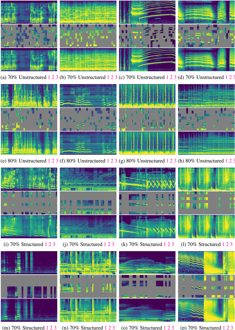<details> <summary>Image 7 Details</summary>  ### Visual Description ## Heatmap Array: Processing Order and Data Structure Impact ### Overview The image displays a 4x4 grid of heatmaps (16 total) comparing visual patterns across different data structure configurations and processing orders. Each heatmap is labeled with a percentage (70% or 80%) and a sequence identifier (1, 2, or 3), suggesting variations in data composition and processing stages. ### Components/Axes - **Rows**: Labeled with percentages (70%, 80%, 70%) indicating data structure composition. - **Columns**: Labeled with "Unstructured" or "Structured" followed by order numbers (1, 2, 3). - **Color Gradient**: Blue-to-yellow scale (no explicit legend, but titles imply quantitative representation). - **Spatial Layout**: - Top row: 70% Unstructured (1, 2, 3) - Second row: 80% Unstructured (1, 2, 3) - Third row: 70% Structured (1, 2, 3) - Bottom row: 70% Structured (1, 2, 3) ### Detailed Analysis 1. **Unstructured Data Trends**: - **70% Unstructured (a, b, c)**: - Horizontal yellow stripes dominate (a), vertical bands (b), and diagonal patterns (c). - 80% Unstructured (e, f, g) shows increased vertical striping (e), fragmented blocks (f), and intensified diagonal gradients (g). - **Structured Data (i, j, k, l, m, n, o, p)**: - Structured 1 (i, m): Vertical yellow bands with gray interruptions. - Structured 2 (j, n): Horizontal yellow stripes with gray gaps. - Structured 3 (k, o, p): Diagonal yellow patterns with varying density. 2. **Order-Specific Patterns**: - Order 1 (a, e, i, m): Vertical/horizontal dominance. - Order 2 (b, f, j, n): Fragmented or alternating patterns. - Order 3 (c, g, k, o, p): Diagonal complexity increases. ### Key Observations - **Color Intensity**: Yellow regions (likely high values) cluster in specific zones, suggesting metric concentration. - **Structured vs. Unstructured**: Structured data heatmaps (i-p) show more geometric regularity than unstructured counterparts. - **Order Impact**: Processing order 3 consistently introduces diagonal complexity across all data types. - **Percentage Effect**: 80% unstructured data (e, f, g) exhibits more chaotic patterns than 70% variants. ### Interpretation The heatmaps likely represent a performance metric (e.g., accuracy, error rate) influenced by: 1. **Data Structure**: Structured data (i-p) shows predictable geometric patterns, implying stability. 2. **Processing Order**: Order 3 introduces diagonal complexity, possibly indicating iterative refinement or error propagation. 3. **Unstructured Data Threshold**: Higher unstructured content (80%) correlates with fragmented patterns, suggesting reduced model confidence or increased noise. The absence of a legend limits quantitative interpretation, but the visual trends strongly suggest that structured data and specific processing orders optimize performance metrics. The diagonal patterns in order 3 heatmaps (c, g, k, o, p) may represent a critical transition phase in the processing pipeline. </details> Table 3: Pre-training (PT) and Fine-tuning (FT) hyperparameters . For augmentation, R: sampling random starting points with cyclic rolling in time; N: adding random noise (signal-to-noise ratio (SNR): 20dB) to spectrograms. For loss functions, BCE: binary cross entropy loss (for multi-label datasets or when using mixup [57]); CE: cross-entropy loss, MSE: mean square error loss. * : We repeat and balance each class to 50% of the size of the unknown class. † : For ViT-S, We use a learning rate of 0.0005 on AS-2M FT and 0.002 on AS-20K FT as we find larger learning rates work better for ViT-S encoder. | | pre-training | | fine-tuning | fine-tuning | fine-tuning | fine-tuning | fine-tuning | |----------------------------------|------------------------------|------------------------------|------------------------------|------------------------------|------------------------------|------------------------------|------------------------------| | Configuration | AS-2M PT | AS-2M | AS-20K | ESC [13] | SPC-2 [52] | SPC-1 | SID [54] | | Optimizer | AdamW [63] | AdamW [63] | AdamW [63] | AdamW [63] | AdamW [63] | AdamW [63] | AdamW [63] | | Optimizer momentum | 1 = 0 . 9 , β 2 = 0 . 95 | 1 = 0 . 9 , β 2 = 0 . 95 | 1 = 0 . 9 , β 2 = 0 . 95 | 1 = 0 . 9 , β 2 = 0 . 95 | 1 = 0 . 9 , β 2 = 0 . 95 | 1 = 0 . 9 , β 2 = 0 . 95 | 1 = 0 . 9 , β 2 = 0 . 95 | | Weight decay | 0.0001 | 0.0001 | 0.0001 | 0.0001 | 0.0001 | 0.0001 | 0.0001 | | Base learning rate | 0.0002 | 0.0002 † | 0.001 | 0.001 | 0.001 | 0.001 | 0.001 | | Learning rate schedule | half-cycle cosine decay [64] | half-cycle cosine decay [64] | half-cycle cosine decay [64] | half-cycle cosine decay [64] | half-cycle cosine decay [64] | half-cycle cosine decay [64] | half-cycle cosine decay [64] | | Minimum learning rate | 0.000001 | 0.000001 | 0.000001 | 0.000001 | 0.000001 | 0.000001 | 0.000001 | | Gradient clipping Warm-up epochs | 3 | 20 | 4 | None 4 | 4 | 1 | 4 | | Epochs | 32 | 100 | 60 | 60 | 60 | 10 | 60 | | Batch size | 512 | 512 | 32 | 64 | 256 | 256 | 64 | | GPUs | 64 | 64 | 4 | 4 | 4 | 4 | 4 | | Weighted sampling | False | True | False | False | False | False * | False | | Weighted sampling size | - | 200,000 | - | - | - | - | - | | Augmentation | R | R | R | R | R+N | R+N | R+N | | SpecAug [48] (time/frequency) | - | 192/48 | 192/48 | 96/24 | 48/48 | 48/48 | 192/48 | | Drop path [65] | 0.0 | 0.1 | 0.1 | 0.1 | 0.1 | 0.1 | 0.1 | | Dropout [66] | 0.0 | 0.0 | 0.0 | 0.0 | 0.0 | 0.0 | 0.0 | | Mixup [57] | 0.0 | 0.5 | 0.5 | 0.0 | 0.5 | 0.5 | 0.0 | | Multilabel | n/a | True | True | False | False | False | False | | Loss Function | MSE | BCE | BCE | CE | BCE | BCE | CE | | Dataset Mean for Normalization | -4.268 | -4.268 | -4.268 | -6.627 | -6.846 | -6.702 | -6.370 | | Dataset Std for Normalization | 4.569 | 4.569 | 4.569 | 5.359 | 5.565 | 5.448 | 3.074 | ## B Experimental Details and Hyperparameter Settings In this section we provide additional experimental details. For audio recordings in each dataset, we pre-process all of them into mono channel under 16K sampling rate for simplicity and consistency between pre-training and fine-tuning tasks. Note that their native sampling rate may not be 16K (there are many 8K or higher sampling rate recordings in AudioSet. Also, video compression by YouTube may up-samples or down-samples the audio tracks of user-uploaded videos). During data loading, we pad or trim the audio length (in seconds) on each dataset as follows: AudioSet: 10, ESC: 5, SPC-1 and SPC-2: 1, SID: 10 seconds. We use a window of 25 ms with a hop length of 10 ms to transform waveform into 128 mel-bank features. The resulting input shapes are: AudioSet: 1 × 1024 × 128 , ESC: 1 × 512 × 128 , SPC: 1 × 128 × 128 , SID: 1 × 1024 × 128 . With different input shapes and audio types, we adjust the hyperparameters and data augmentation for each task respectively. We summarize the pre-training (AS-2M PT) and fine-tuning details on each dataset in Table 3. We adopt most of the default hyper-parameters used in MAE [1]. Note that the effective learning rate ( lr eff) depends on the base learning rate ( lr base) and the batch size. Precisely, lr eff = lr base ∗ batch size 256 . When the dataset is multi-label or the mixup [57] augmentation is enabled, we use binary crossentropy loss (BCE) as the fine-tuning objective without label smoothing [67].We also experimented using strong data augmentations ( e.g ., mixup [57], SpecAug [57], and CutMix [56]) for pre-training but found the resulting performance similar or worse (especially for CutMix which resulted in ∼ 0.5 mAP degrade in AudioSet-2M). Therefore we discard these strong data augmentations in the pre-training phase by default. To perform importance sampling when fine-tuning on the unbalanced AudioSet-2M, following prior works, we apply a weighted sampler. We set the probability of sampling a sample proportional to the inverse frequency of its labels, where the label frequency is estimated over the training set. Specifically, for a instance i in a dataset D with a label pool C , its sampling weight is proportional to ∑ c i ∈ C w c , where w c = 1000 ∑ i ∈ D c i + and = 0 . 01 is set to avoid underflow in majority classes as in [10]. In each fine-tuning epoch on AS-2M, we sample 200K instances ( ∼ 10% of AudioSet-2M) without replacement in avoidance of duplicated samples in a batch and repeating samples within an epoch. We fine-tune for 100 epochs, which aggregate to ∼ 10 full epochs of AudioSet-2M. Proper normalization for audio is important to avoid pre-training fine-tuning discrepancy. We use the training split of each end task to estimate dataset-wise mean and standard deviation The code, scripts, and pretrained models for reproducibility are at https://github.com/facebookresearch/AudioMAE . ## C Additional Experiments In this section, we extend our experimental investigation of Audio-MAE to include additional results that are not covered in the main paper. First (§C.1), on ESC-50, we report and compare model performance under an additional round of supervised pre-training on labeled AudioSet-2M (models marked with † in Table 2 of the main paper). Second (§C.2), we include additional qualitative results on packet loss concealment (PLC) as a preliminary case study on practically useful downstream tasks for the decoder in Audio-MAE, and demonstrate its potential impact for generative applications. Third (§C.3), we share some negative results when we tried incorporating contrastive objectives for Audio-MAE. Our findings suggest that using reconstruction objective alone is sufficient. ## C.1 ESC-50 with AudioSet-2M Supervised Pre-training ESC-50 is designed for environmental sound classification. Besides the pre-training setup introduced in the original paper, we further study a widely compared setup where the models are additionally supervisedly pre-trained with AudioSet data and labels before fine-tuning on ESC-50. Table 4 summarizes the results under this setup where our Audio-MAE achieves state of the art accuracy with the additional AudioSet-2M supervised pre-training. Note that our model is still audio-only and uses no ImageNet data (IN-SL). Table 4: Comparison with other state-of-the-art models on ESC-50 with an additional round of supervised pre-training on AudioSet (AS-SL). SSL: self-supervised learning. We gray-out the models with out-of-domain pre-training on ImageNet (IN). | Model | Backbone | Pre-training | ESC-50 FT | |--------------------|------------|----------------|-------------| | ERANN [58] | CNN | AS-SL | 96.1 | | PANN [59] | CNN | AS-SL | 94.7 | | AST [10] | DeiT-B | IN-SL, AS-SL | 95.6 | | HTS-AT [29] | Swin-B | IN-SL, AS-SL | 97 | | PASST [28] | DeiT-B | IN-SL, AS-SL | 96.8 | | Audio-MAE (global) | ViT-B | AS-SSL, AS-SL | 96.9 | | Audio-MAE (local) | ViT-B | AS-SSL, AS-SL | 97.4 | ## C.2 Qualitative Results for a practical generation task Packet Loss Concealment (PLC) is a widely deployed technique to alleviate side effects from missing or corrupted packets in Voice over IP (VoIP) applications ( e.g ., video conferencing, Bluetooth earbuds, wireless virtual reality headset, etc .) When an encoded speech is sent as a sequence of VoIP packets over a network, these packets may get lost or be corrupted during the transmission, resulting in undesirable low quality speech. To this end, various PLC techniques has been developed. The recent approaches substitute the corrupted waveform segments by either replacing the corrupted waveform segments with other intact segments base on the acoustic pitch detected, or via inpainting with RNN-based [68], CNN-based [69], or autoencoding-based [70, 71] reconstruction. In this section, we qualitatively demonstrate how Audio-MAE could potentially be applied for PLC to recover corrupted waveform segments with its encoder-decoder architecture. In Fig. 8, we simulate two time-corrupted speech recordings by masking speech in time and perform reconstruction with Audio-MAE. In practice, a PLC system may exploit packet checksums to identify corrupted or missing packets and mask them. The PLC problem then can be viewed as a special case (time-only, structured masking) of Audio-MAE. As shown in both cases, the Audio-MAE decoder produces reasonable speech reconstruction. We leave the in-depth study and analysis of generative tasks ( e.g . PLC and speech bandwidth expansion (BWE) [72, 54]) as the future work. Figure 8: Qualitative Results for Packet Loss Concealment with Audio-MAE Decoder . Simulations of 25% packet loss rate in time for two speech recordings. In each group, we show the original spectrogram(left) and time(right) sequence (1, top), corrupted input with packet loss (2, middle), and Audio-MAE restoration (3, bottom). The spectrogram size is 1024 × 128; patch size is 16 × 16. Please click (1 2 3) for audible .wav s. 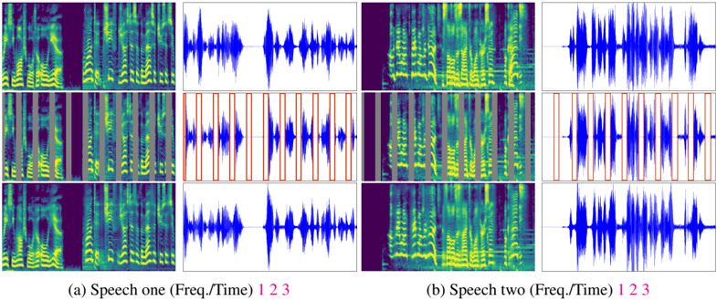<details> <summary>Image 8 Details</summary>  ### Visual Description ## Spectrogram and Waveform Analysis: Speech Comparison ### Overview The image presents a comparative analysis of two speech samples (Speech one and Speech two) across three time-frequency segments (1, 2, 3). Each segment includes a spectrogram (left) and corresponding waveform (right), with annotations highlighting specific features. --- ### Components/Axes 1. **Spectrogram Axes**: - **X-axis**: Time (s) - Linear scale from 0 to ~3 seconds. - **Y-axis**: Frequency (Hz) - Logarithmic scale from ~0 to ~4 kHz. - **Color Scale**: Intensity (dB) - Dark blue (low) to bright yellow (high). 2. **Waveform Axes**: - **X-axis**: Time (s) - Linear scale matching spectrogram. - **Y-axis**: Amplitude (normalized) - Vertical displacement of audio signal. 3. **Annotations**: - **Red Boxes**: Highlighted intervals in Speech two, Subsection 2 (Time: ~0.5–1.5s). - **Subsection Labels**: "1", "2", "3" in magenta, positioned at bottom-left of spectrograms. 4. **Legend**: - **Top-right corner**: - Blue: Waveform (Speech one/two). - Green/Yellow: Spectrogram intensity. --- ### Detailed Analysis #### Speech one - **Subsection 1**: - Spectrogram: Dominant vertical stripes at ~1–2 kHz, indicating sustained vowel sounds. - Waveform: Moderate amplitude peaks (~0.5–1.0) with consistent periodicity. - **Subsection 2**: - Spectrogram: Reduced intensity at ~500 Hz, suggesting transitional phonemes. - Waveform: Lower amplitude (~0.2–0.4) with irregular oscillations. - **Subsection 3**: - Spectrogram: Broadband noise (0.5–4 kHz) with intermittent peaks, likely fricatives or background noise. - Waveform: High-amplitude bursts (~1.2–1.8) with chaotic patterns. #### Speech two - **Subsection 1**: - Spectrogram: Similar vertical stripes to Speech one but narrower bandwidth (~1.5–2.5 kHz). - Waveform: Slightly higher amplitude (~0.6–1.1) with sharper peaks. - **Subsection 2** (Highlighted): - Spectrogram: Red boxes mark intervals with abrupt frequency drops (~200 Hz) and intensity spikes (~3 kHz). - Waveform: Sharp transients (~0.8–1.2) with irregular spacing. - **Subsection 3**: - Spectrogram: More pronounced noise floor (0.3–3 kHz) compared to Speech one. - Waveform: Lower overall amplitude (~0.3–0.7) with reduced peak sharpness. --- ### Key Observations 1. **Subsection 2 Highlights**: - Speech two exhibits abrupt spectral changes (red boxes), potentially indicating phonetic boundaries or articulation errors. - Waveform transients align with spectrogram intensity spikes, suggesting plosive consonants or glottal stops. 2. **Subsection 3 Variability**: - Speech one shows higher energy in broadband noise, possibly due to environmental interference. - Speech two’s reduced amplitude may reflect quieter articulation or post-processing. 3. **Temporal Consistency**: - Both speeches maintain similar temporal alignment (3-second duration), but Speech two’s waveforms display greater amplitude variability. --- ### Interpretation The data suggests a comparative study of speech characteristics, possibly for phonetic analysis or speaker identification. The highlighted intervals in Speech two (Subsection 2) may represent critical features for distinguishing speech patterns, such as dialectal differences or pathological speech markers. The spectrogram-waveform correlation confirms that spectral features (e.g., formants, noise) directly map to temporal amplitude variations. Subsection 3’s noise differences could indicate varying recording conditions or speaker-specific prosody. The use of color coding enhances interpretability by decoupling time-frequency intensity from amplitude visualization. </details> ## C.3 Negative Results: Directions that did not work well Additional Contrastive Objective We examined using additional contrastive objectives in the pretraining phase but do not find them helpful empirically. Similar to SS-AST [18] and Wave2vec 2.0 [33], we apply InfoNCE [46] loss over masked tokens of an instance. Specifically, let x i , i = 1 . . . N denotes the values of i -th masked spectrogram patch where N is the number of masked patches in an instance. ( e.g ., rounded N = 102 under 80% masking over 64 × 8 spectrogram patches of a 10-second audio recording.) And let c i denotes its corresponding contextualized embedding projected by a separated decoder head. We investigate the following contrastive objective: $$L _ { c } = - \frac { 1 } { N } \sum _ { i = 1 } ^ { N } \log \frac { e ^ { i x _ { i } } } { \sum _ { j = 1 } ^ { N } e ^ { i x _ { j } } }$$ Intuitively, L c draws closer patches with their contextualized embeddings (positive pairs) at each masked position while contrasting and pushing away mismatched ones (negative pairs) from all masked patches. For the reconstructive objective, let ˆ x i , i = 1 . . . N be the reconstruction of i -th masked spectrogram patch generated by the reconstruction head of our Audio-MAE decoder. The original reconstruction objective L r in Audio-MAE is formally defined as: $$L _ { r } = \frac { 1 } { N } \sum _ { i = 1 } ^ { N } ( x _ { i } - x ) ^ { 2 } .$$ We consider three setups: (1) Using the reconstructive objective ( L r ) alone (the default setup); (2) using the contrastive objective ( L c ) alone; (3) multi-tasking with both the reconstructive and contrastive objectives ( L r + αL c ), where α is the hyper-parameter that balances two objectives. Table 5 shows the results: We see that the reconstruction objective L r alone is sufficient and yields the best performance. Empirically, we do not observe improvement with contrastive objectives alone or under the multi-task setup (the best α is 0.2 in our experiments). L c and L r do not work complementarily in Audio-MAE. ## D Limitations We think there are few direct limitations of this work. The data scale is one of them. AudioSet used by Audio-MAE is around two orders of magnitude smaller than the text corpus used in the language [3, 5, 4] counterparts. Another limitation is duration of each sample: the 10-second recordings in AudioSet are short and thus distant temporal dependencies in audio may not be properly learned yet. Further, as AudioSet is unbalanced and there are many audio types beyond the 527 classes annotated in AudioSet, Audio-MAE could be sub-optimal when transferring to tasks concerning rare or unseen audio events. Lastly, while Audio-MAE has greatly improved the efficiency of large-scale self-supervised learning, modeling lengthy audio and high-dimensional data with Transformers is computationally demanding. Table 5: Impact of contrastive objective . | Objective | AS-20K AS-2M | AS-20K AS-2M | |---------------------------------------------|----------------|----------------| | Reconstruction ( L r ) | 37.1 | 47.3 | | Contrastive ( L c ) | 36.4 | 46.6 | | Contrastive + Reconstruction ( L r + αL c ) | 36.8 | 46.8 |