2207.14070v2

## Full counting statistics of interacting lattice gases after an expansion: The role of the condensate depletion in the many-body coherence Ga´ etan Herc´ e, 1, ∗ Jan-Philipp Bureik, 1, ∗ Antoine T´ enart, 1 Alain Aspect, 1 Alexandre Dareau, 1 and David Cl´ ement 1 1 Universit´ e Paris-Saclay, Institut d'Optique Graduate School, CNRS, Laboratoire Charles Fabry, 91127, Palaiseau, France (Dated: December 1, 2022) We study the full counting statistics (FCS) of quantum gases in samples of thousands of interacting bosons, detected atom-by-atom after a long free-fall expansion. In this far-field configuration, the FCS reveals the many-body coherence from which we characterize iconic states of interacting lattice bosons by deducing the normalized correlations g ( n ) (0) up to the order n = 6. In Mott insulators, we find a thermal FCS characterized by perfectly-contrasted correlations g ( n ) (0) = n !. In interacting Bose superfluids, we observe small deviations to the Poisson FCS and to the ideal values g ( n ) (0) = 1 expected for a pure condensate. To describe these deviations, we introduce a heuristic model that includes an incoherent contribution attributed to the depletion of the condensate. The predictions of the model agree quantitatively with our measurements over a large range of interaction strengths, that includes the regime where the condensate is strongly depleted by interactions. These results suggest that the condensate component exhibits a full coherence g ( n ) (0) = 1 at any order n up to n = 6 and at arbitrary interaction strengths. The approach demonstrated here is readily extendable to characterize a large variety of interacting quantum states and phase transitions. ## I. INTRODUCTION The dispersion of a physical quantity contains important information, beyond that obtained from its average value. The analysis of quantum and thermal noise is central in various systems, ranging from quantum electronics [1] and quantum optics [2] to quantum gases [3-5]. The ultimate precision on the measurement of noise is given by the full counting statistics (FCS) [6], which is obtained with single-particle-resolved detection methods that provide the number of particles detected in a given time and/or space interval. These methods yield highorder moments of the particle number beyond the variance. Probing high-order moments is a means to study quantum phase transitions [7-9], universality [10, 11], entanglement properties [12] or out-of-equilibrium dynamics [13]. The FCS has indeed successfully characterized various phenomena in mesoscopic conductors [1, 6, 14, 15], Rydberg [16-18] and non-interacting [19, 20] atomic gases. From a Quantum Information perspective, the FCS holds great promises for large ensembles of particles. In contrast to a full-state tomography [21], the FCS is accessible even in large systems as it probes information only about the diagonal part of the n -body density matrices ( i.e. populations). Although it does not contain the total information about the quantum state, the FCS is sufficient to identify many quantum states without resorting to a consuming tomography. A similar idea was introduced by R. Glauber to characterize light sources from photon correlations at any order [22]. For Gaussian states, for which the Wigner function is positive [2], measuring the FCS or the magnitudes of correlation functions ∗ These authors contributed equally to this work. is indeed equivalent. In strongly-correlated quantum states characterized by non-Gaussian Wigner functions, measuring the FCS and many-body correlations is expected to reveal the nontrivial nature of such states [5, 23-25]. Moreover, recent works have shown that applying random unitary transformations before measuring the FCS provides access to non-diagonal correlators [26, 27], further motivating the development of experimental approaches to the FCS in strongly-interacting quantum systems. In this letter, we report the measurement of the full counting statistics in large three-dimensional (3D) ensembles ( ∼ 5 × 10 3 atoms) of interacting lattice bosons after a free-fall expansion (see Fig. 1(a)). This configuration is analogous to the far-field regime of light propagation during which interferences take place, and after which the FCS identifies quantum states through their many-body coherence [28]. In quantum gases, farfield - or momentum - correlations have been measured with single-atom detection in non-interacting and nondegenerate bosonic [29, 30] and fermionic [31, 32] gases and in Bose-Einstein condensates [33]. More recently momentum correlations in interacting lattice bosons [3436] and interacting fermions [37] were studied. However, the FCS has thus far been measured only in 1D noninteracting bosons [30]. Here, we study various regimes of interacting 3D Bose gases across the superfluid-to-Mott phase transition, extending the measurement of manybody correlations to the strongly-interacting regime. This allows us to reveal the role of the depletion of the condensate in the many-body coherence properties of interacting Bose superfluids. We characterize the FCS by measuring the probability distribution of the atom number N Ω falling in a small voxel V Ω (see Fig. 1(a)). 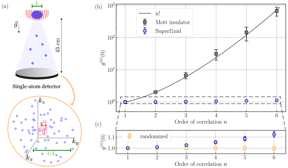As explained below, a crucial asset of our work is the ability to probe many-body coherence into volumes smaller than that occupied by one FIG. 1. (a) Free-fall expansion of interacting quantum gases of metastable Helium-4 atoms from a three-dimensional optical lattice, yielding the 3D positions of individual atoms in the momentum space. The full counting statistics P ( N Ω ) describes the statistics of the atom number N Ω detected in a small voxel of volume V Ω ∼ ( δk ) 3 (red cube). To reveal the many-body coherence properties of the trapped gas of size L , δk is chosen such that δk 2 π/L . (b) Magnitudes g ( n ) ( 0 ) of n -body correlations as a function of the order n , measured in a Mott insulator (black squares) and a superfluid (blue circles). The black solid line is the prediction for thermal states, g ( n ) (0) = n !. (c) g ( n ) ( 0 ) in the superfluid (blue circles) and in a randomized set (orange squares, see main text). A deviation to the prediction for a pure coherent state, g ( n ) (0) = 1, is observed. <details> <summary>Image 1 Details</summary>  ### Visual Description ## Chart/Diagram Type: Experimental Setup & Correlation Function Plots ### Overview The image presents an experimental setup for observing single atoms and corresponding plots of the correlation function g⁽²⁾(0) versus the order of correlation *n* for different quantum phases of matter: Mott insulator, superfluid, and a randomized control. The setup involves a laser beam (indicated by the blue cone) focused onto a sample, and a single-atom detector. ### Components/Axes **(a) Experimental Setup Diagram:** * **Labels:** "L" (length scale), "g" (gravitational acceleration direction), "43 cm" (distance), "Single-atom detector". * **Diagram Components:** Laser beam focus, atom positions, single-atom detector, k-space representation with wavevectors k_x, k_y, k_z, and δk. * **k-space:** A cube with dimensions 1/L. **(b) Correlation Function Plot:** * **X-axis:** "Order of correlation n" (scale from 1 to 6). * **Y-axis:** "g⁽²⁾(0)" (logarithmic scale from 10⁰ to 10³). * **Legend:** * Black line: "n!" * Gray square: "Mott insulator" * Blue circle: "Superfluid" * **Error Bars:** Present for all data points. **(c) Correlation Function Plot (Randomized):** * **X-axis:** "Order of correlation n" (scale from 1 to 6). * **Y-axis:** "g⁽²⁾(0)" (linear scale from 1.0 to 1.2). * **Legend:** * Red square: "randomized" * Blue circle: "Superfluid" * **Error Bars:** Present for all data points. ### Detailed Analysis or Content Details **(a) Experimental Setup:** The diagram shows a laser beam focused onto a region containing atoms. The length scale "L" is indicated on the beam. The distance from the beam focus to the single-atom detector is approximately 43 cm. The k-space representation shows the distribution of wavevectors, with a cube representing the reciprocal lattice space with dimensions 1/L. **(b) Correlation Function Plot:** * **n! (Black Line):** The line exhibits an exponential increase with increasing *n*. * n=1: g⁽²⁾(0) ≈ 1.0, with error bar spanning approximately 0.8 to 1.2. * n=2: g⁽²⁾(0) ≈ 2.0, with error bar spanning approximately 1.5 to 2.5. * n=3: g⁽²⁾(0) ≈ 6.0, with error bar spanning approximately 4.0 to 8.0. * n=4: g⁽²⁾(0) ≈ 24.0, with error bar spanning approximately 18.0 to 30.0. * n=5: g⁽²⁾(0) ≈ 120.0, with error bar spanning approximately 80.0 to 160.0. * n=6: g⁽²⁾(0) ≈ 720.0, with error bar spanning approximately 500.0 to 900.0. * **Mott Insulator (Gray Squares):** The data points are approximately constant around g⁽²⁾(0) ≈ 1.0, with small fluctuations within the error bars. * n=1: g⁽²⁾(0) ≈ 1.0, with error bar spanning approximately 0.8 to 1.2. * n=2: g⁽²⁾(0) ≈ 1.2, with error bar spanning approximately 0.9 to 1.5. * n=3: g⁽²⁾(0) ≈ 1.1, with error bar spanning approximately 0.8 to 1.4. * n=4: g⁽²⁾(0) ≈ 1.3, with error bar spanning approximately 1.0 to 1.6. * n=5: g⁽²⁾(0) ≈ 1.1, with error bar spanning approximately 0.9 to 1.3. * n=6: g⁽²⁾(0) ≈ 1.2, with error bar spanning approximately 1.0 to 1.4. * **Superfluid (Blue Circles):** The data points are approximately constant around g⁽²⁾(0) ≈ 1.0, with small fluctuations within the error bars. * n=1: g⁽²⁾(0) ≈ 1.0, with error bar spanning approximately 0.8 to 1.2. * n=2: g⁽²⁾(0) ≈ 1.0, with error bar spanning approximately 0.8 to 1.2. * n=3: g⁽²⁾(0) ≈ 1.0, with error bar spanning approximately 0.8 to 1.2. * n=4: g⁽²⁾(0) ≈ 1.0, with error bar spanning approximately 0.8 to 1.2. * n=5: g⁽²⁾(0) ≈ 1.0, with error bar spanning approximately 0.8 to 1.2. * n=6: g⁽²⁾(0) ≈ 1.1, with error bar spanning approximately 0.9 to 1.3. **(c) Correlation Function Plot (Randomized):** * **Randomized (Red Square):** The data points are approximately constant around g⁽²⁾(0) ≈ 1.1, with small fluctuations within the error bars. * n=1: g⁽²⁾(0) ≈ 1.1, with error bar spanning approximately 0.9 to 1.3. * n=2: g⁽²⁾(0) ≈ 1.1, with error bar spanning approximately 0.9 to 1.3. * n=3: g⁽²⁾(0) ≈ 1.1, with error bar spanning approximately 0.9 to 1.3. * n=4: g⁽²⁾(0) ≈ 1.1, with error bar spanning approximately 0.9 to 1.3. * n=5: g⁽²⁾(0) ≈ 1.1, with error bar spanning approximately 0.9 to 1.3. * n=6: g⁽²⁾(0) ≈ 1.1, with error bar spanning approximately 0.9 to 1.3. * **Superfluid (Blue Circles):** The data points are approximately constant around g⁽²⁾(0) ≈ 1.0, with small fluctuations within the error bars. ### Key Observations * The correlation function for the "n!" series increases dramatically with the order of correlation *n*, indicating strong correlations between atoms. * Both the Mott insulator and superfluid phases exhibit a nearly constant correlation function around g⁽²⁾(0) ≈ 1.0, suggesting weak correlations. * The randomized data shows a slightly elevated correlation function around g⁽²⁾(0) ≈ 1.1, indicating some residual correlations. * The error bars are relatively large, especially for the "n!" series, indicating significant uncertainty in the measurements. ### Interpretation The data demonstrates the distinct correlation properties of different quantum phases of matter. The exponential increase in the correlation function for the "n!" series likely represents a theoretical benchmark or a reference for comparison. The constant correlation function for the Mott insulator and superfluid phases suggests that atoms in these phases are either localized (Mott insulator) or delocalized (superfluid), resulting in weak correlations. The randomized data provides a control to assess the level of correlations present in the system due to experimental artifacts or residual interactions. The large error bars suggest that the measurements are challenging and require further refinement. The difference between the superfluid and randomized data suggests that the superfluid phase exhibits a degree of coherence not present in the randomized system. The experimental setup provides a means to probe the quantum properties of atoms and distinguish between different phases of matter based on their correlation characteristics. </details> mode in momentum space, i.e. V Ω (2 π/L ) 3 with L the in-trap size of the gas. This possibility is given by the large quantum efficiency of our detector( η = 0 . 53(2)) [36]. Furthermore, we determine the magnitudes g ( n ) (0) of correlation functions (up to n = 6) from the factorial moments of N Ω [38]. As shown in Fig. 1(b), g ( n ) (0) is found to vary by several orders of magnitude between the superfluid and the Mott insulator states. Interestingly, we observe small deviations to the predictions for a pure condensate in Bose superfluids (see Fig. 1(c)), which is in contrast to a previous work [33]. Since ab-initio calculations of many-body correlations with thousands of interacting atoms are beyond state-of-the-art numerics, we interpret our findings from introducing a heuristic model that includes the contribution of the condensate depletion. Its hypotheses rely on an intuitive physical picture in the weakly-interacting regime but, surprisingly, its predictions are in quantitative agreement with our observations even in the strongly-interacting regime. Our observations lead us to conclude that the condensate component exhibits a full coherence, g ( n ) (0) = 1 (at least up to n = 6), at arbitrary strength of interactions. ## II. FULL COUNTING STATISTICS (FCS) OF PURE-STATE BECS AND MOTT INSULATORS Textbook descriptions of Bose-Einstein Condensates (BECs) and Mott insulators are based on pure states. Bose-Einstein condensation is associated with the breaking of phase symmetry [39] whose complex order parameter defines a coherent state describing the BEC. In a grand canonical approach, coherent states have a Poisson counting statistics, P ( N Ω ) = 〈 N Ω 〉 N Ω exp[ -〈 N Ω 〉 ] /N Ω ! where N Ω is the number of detected bosons in the considered volume V Ω , and a full coherence g ( n ) = 1 at any order n of normalized correlations either in position or in momentum space [22]. In our experiment, we determine $$e \text subscript { e- } \quad g ^ { ( n ) } ( 0 ) = g ^ { ( n ) } ( k , k , \dots , k ) = \frac { \langle [ a ^ { \dagger } ( k ) ] ^ { n } [ a ( k ) ] ^ { n } \rangle } { \langle a ^ { \dagger } ( k ) a ( k ) \rangle ^ { n } } , \quad ( 1 )$$ where k is the momentum at which correlations are evaluated, i.e. where the volume V Ω is located. For a pure coherent state we expect g ( n ) (0) = 1 at all orders. In contrast, a 'perfect' Mott insulator - a uniform Mott insulator at zero temperature - is thought of as a Fock state in the (in-trap) position basis. In the momentum basis, which is probed after a long expansion from the trap, it is expected to exhibit thermal statistics [34, 40, 41]. This is because far-field correlations reflect multi-particle interferences from a discrete series of emitters (atoms in the lattice sites) with no coherence between the sites (no tunnelling), a situation analog to that of light emitted by many incoherent sources. Thermal states are characterized by a counting statistics P ( N Ω ) = (1 -q ) q N Ω where q = 〈 N Ω 〉 / 1 + 〈 N Ω 〉 and g ( n ) ( k , k , ...., k ) = n ! [42]. Note that both the Poisson and the thermal FCS are fully determined by a single parameter, the average number of particles 〈 N Ω 〉 , as a result of the Gaussian character of their quantum state [2]. For Gaussian states, a detection efficiency η smaller than one does not affect the measurement of the FCS - nor that of g ( n ) . Whether these many-body coherence properties of pure states describe experiments is not granted. On the one hand, pure states are approximated descriptions of states produced in an experiment because of the coupling to the environment. Determining the level e.g. the order n of correlations -up to which a description in terms of pure states is valid provides a quantitative certification of experimental realizations. In the context of the development of platforms for quantum technologies, such a certification is of interest. On the other hand, the properties of quantum states produced at thermodynamical equilibrium are affected by constraints on macroscopic quantities. In the canonical (or microcanonical) ensemble there are no fluctuations of the total BEC atom number N BEC in a gas of non-interacting bosons at zero temperature [43]: N BEC is fixed to the total atom number, N BEC = N . The statistics of N BEC is therefore not that of a coherent state [44]. To alleviate such global constraints and mimic a grand canonical ensemble, one may probe the FCS in a volume V Ω much smaller than that, V BEC , occupied by the BEC. The volume V BEC -V Ω ∼ V BEC then serves as a reservoir for the sub-volume V Ω where the number of bosons N Ω N may fluctuate [45]. Measuring the FCS in small sub-volumes V Ω is also crucial if correlation functions g ( n ) ( k , k ′ , ...., k ′′ ) are bell shaped with widths l ( n ) c . While this is not an issue for a coherent state, which is fully coherent over the entire volume it occupies, correlation functions of a thermal state must be probed in a volume V Ω much smaller than the coherence volume V ( n ) c = [ l ( n ) c ] 3 , since particles distant by l ( n ) c are essentially uncorrelated. This is well known in the case of the Hanbury-Brown and Twiss effect where the property g (2) ( k , k ′ ) = 2 is expected only if | k -k ′ | is less that the width of the far-field diffraction pattern associated with the source size. In the far-field, the correlation lengths of Mott insulators and of thermal Bose gases are set by the inverse in-trap size, l ( n ) c ∼ 2 π/L [34, 35]. As a result, observing fully-contrasted n -body correlations requires using V Ω (2 π/L ) 3 . This condition also ensures the above-mentioned criterion on probing BECs as the volume occupied by the BEC in the momentum space is set by ∆ k ∼ 1 . 6 /L [46]. With these consider- ations in mind, we compute the magnitudes g ( n ) (0) of correlation functions in a volume V Ω ∼ ( δk ) 3 of the momentum space such that δk × L 2 π (see Fig. 1(a)). As illustrated below, this choice is essential to correctly reveal the full statistical properties. ## III. MEASUREMENT OF THE FCS IN MOTT INSULATORS AND BOSE SUPERFLUIDS Our measurement of the FCS in the far-field exploits the 3D atom-by-atom detection of metastable Helium4 ( 4 He ∗ ) after a long free-fall expansion [47, 48] (see Fig. 1(a)). The detection efficiency is η = 0 . 53(2) per atom, with negligible dark counts. For an individual run, we register the number of atoms in each of the voxels V Ω mentioned above, and we use more than 2000 runs to obtain the probability distribution in each voxel. We apply this approach to probe equilibrium quantum states of 4 He ∗ atoms loaded in the lowest energy-band of a threedimensional (3D) optical lattice [49]. The lattice implements the 3D Bose-Hubbard Hamiltonian whose main parameters are the tunnelling amplitude J and the onsite (repulsive) interaction U . 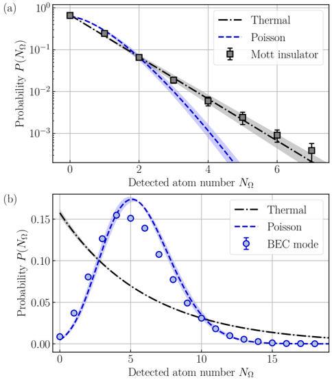We first investigate the thermal nature of Mott insulators in the momentum space. We realize Mott insulators with N = 6 . 5(6) × 10 3 atoms at U/J = 76, which corresponds to a lattice filling of one atom per site at the trap center [34] and an almost uniform filling of the first Brillouin zone in the momentum space. To compute the counting statistics in this first set of experiments, we divide the first Brillouin zone into cubic voxels V Ω of size δk = 6 × 10 -2 k d and average the probability distributions measured over all these voxels. Here k d = 2 π/d is the momentum associated with the lattice spacing d = 775 nm and the size δk is comparable to that of one mode in momentum space, δk ∼ 2 π/L (see Appendix A). The resulting FCS of the Mott state is shown in Fig. 2(a). It is found to be in excellent agreement with a thermal statistics whose average atom number is that measured in the experiment, 〈 N Ω 〉 = 0 . 46(5). The statistical properties of the Mott state are also revealed through the magnitudes g ( n ) (0) of the normalized correlation functions, as an alternative to the probability distribution P ( N Ω ). We determine g ( n ) (0) from the factorial moments of the detected atom number N Ω in small voxels V Ω with δk 2 π/L (see Appendix B), $$g ^ { ( n ) } ( 0 ) = \frac { \langle N _ { \Omega } ( N _ { \Omega } - 1 ) \dots ( N _ { \Omega } - n + 1 ) \rangle } { \langle N _ { \Omega } \rangle ^ { n } } , \quad ( 2 )$$ transposing a well-known approach in quantum optics [50]. The correlation functions of quantum optics [22] are defined with normal ordering of the destruction operators since a detected photon is destroyed. Even if it is not always emphasized, the correlation functions in quantum optics are indeed calculated from the factorial moments, and it is remarkable that the corresponding quantities in classical statistics are also based on factorial moments FIG. 2. (a) Full Counting statistics P ( N Ω ) to find N Ω atoms in a small volume V Ω of the momentum space when probing a Mott insulator with unity filling (black circles). The predictions for thermal ( resp. Poissonian) statistics is shown as a dashed-dotted black ( resp. dashed blue) line. We use the measured value 〈 N Ω 〉 = 0 . 46(5) for the theoretical predictions (the shaded areas reflect the uncertainty on 〈 N Ω 〉 ). The error bars denote the statistical uncertainty (standard deviation) estimated with the bootstrapping method. (b) Same as (a) in the BEC mode ( k = 0 ) of interacting lattice superfluids (SF) with U/J = 5. The mean atom number is 〈 N Ω 〉 = 5 . 3(2). Error bars are smaller than the dots. <details> <summary>Image 2 Details</summary>  ### Visual Description \n ## Chart: Atom Number Distribution ### Overview The image presents two charts (labeled (a) and (b)) displaying the probability distribution of detected atom numbers. Both charts share the same x-axis label ("Detected atom number NΩ") and y-axis label ("Probability P(NΩ)"), but differ in their y-axis scale (logarithmic in (a) and linear in (b)). Each chart compares experimental data (represented by markers with error bars) to theoretical distributions: Thermal and Poisson. Chart (a) focuses on the Mott insulator state, while chart (b) focuses on the BEC mode. ### Components/Axes * **X-axis:** "Detected atom number NΩ", ranging from approximately 0 to 6 in (a) and 0 to 12 in (b). * **Y-axis (a):** "Probability P(NΩ)", logarithmic scale, ranging from approximately 10⁻³ to 10⁰. * **Y-axis (b):** "Probability P(NΩ)", linear scale, ranging from approximately 0 to 0.16. * **Legend:** * **Chart (a):** * Black dashed line: "Thermal" * Blue dashed line: "Poisson" * Gray square markers with error bars: "Mott insulator" * **Chart (b):** * Black dashed line: "Thermal" * Blue dashed line: "Poisson" * Blue circle markers with error bars: "BEC mode" * **Grid:** Both charts have a grid for easier value reading. ### Detailed Analysis or Content Details **Chart (a): Mott Insulator** * **Mott Insulator (Gray Squares):** The data points show a decreasing probability as the detected atom number increases. * NΩ = 0: P(NΩ) ≈ 0.95 ± 0.05 * NΩ = 1: P(NΩ) ≈ 0.30 ± 0.05 * NΩ = 2: P(NΩ) ≈ 0.10 ± 0.02 * NΩ = 3: P(NΩ) ≈ 0.03 ± 0.01 * NΩ = 4: P(NΩ) ≈ 0.01 ± 0.005 * NΩ = 5: P(NΩ) ≈ 0.003 ± 0.002 * NΩ = 6: P(NΩ) ≈ 0.001 ± 0.001 * **Thermal (Black Dashed):** Starts at approximately 1 and decreases slowly with increasing NΩ. * **Poisson (Blue Dashed):** Starts at approximately 1 and decreases more rapidly than the Thermal distribution. **Chart (b): BEC Mode** * **BEC Mode (Blue Circles):** The data points show an initial increase in probability, reaching a maximum around NΩ = 4, and then decreasing. * NΩ = 0: P(NΩ) ≈ 0.02 ± 0.01 * NΩ = 1: P(NΩ) ≈ 0.06 ± 0.01 * NΩ = 2: P(NΩ) ≈ 0.10 ± 0.01 * NΩ = 3: P(NΩ) ≈ 0.14 ± 0.01 * NΩ = 4: P(NΩ) ≈ 0.15 ± 0.01 * NΩ = 5: P(NΩ) ≈ 0.11 ± 0.01 * NΩ = 6: P(NΩ) ≈ 0.07 ± 0.01 * NΩ = 7: P(NΩ) ≈ 0.04 ± 0.01 * NΩ = 8: P(NΩ) ≈ 0.02 ± 0.01 * NΩ = 9: P(NΩ) ≈ 0.015 ± 0.005 * NΩ = 10: P(NΩ) ≈ 0.01 ± 0.005 * NΩ = 11: P(NΩ) ≈ 0.005 ± 0.003 * NΩ = 12: P(NΩ) ≈ 0.003 ± 0.002 * **Thermal (Black Dashed):** Decreases monotonically with increasing NΩ. * **Poisson (Blue Dashed):** Increases initially, reaches a maximum around NΩ = 2, and then decreases. ### Key Observations * In Chart (a), the Mott insulator data deviates significantly from both the Thermal and Poisson distributions, especially at higher atom numbers. The Mott insulator distribution decays much faster than the Poisson distribution. * In Chart (b), the BEC mode data shows a clear peak, indicating a preferred atom number. The BEC mode distribution is significantly different from both the Thermal and Poisson distributions. * The logarithmic scale in Chart (a) emphasizes the differences in the tail of the distribution, while the linear scale in Chart (b) highlights the peak. ### Interpretation These charts demonstrate the distinct statistical properties of different quantum states of atoms. Chart (a) shows that the Mott insulator state exhibits a strong suppression of atom number fluctuations, deviating from the predictions of both thermal and Poisson statistics. This is consistent with the theoretical expectation that Mott insulators are characterized by a fixed number of atoms per site. Chart (b) shows that the BEC mode exhibits a peak in the probability distribution, indicating a tendency for atoms to condense into the same quantum state. The shape of the BEC mode distribution is also different from both thermal and Poisson statistics, reflecting the unique quantum mechanical properties of Bose-Einstein condensates. The comparison to the Poisson distribution is particularly relevant, as the Poisson distribution describes the statistics of independent events, while the Mott insulator and BEC mode represent correlated quantum states. The error bars on the experimental data indicate the uncertainty in the measurements, and the agreement between the experimental data and the theoretical predictions provides strong evidence for the validity of the theoretical models. The use of two different y-axis scales allows for a more comprehensive comparison of the distributions, highlighting both the overall shape and the details of the tails. </details> [51]. In the experiments reported here, each detected He ∗ atom is destroyed ( i.e. it decays to its ground-state) and the results of quantum optics are directly transposed. As explained in section II, fully-contrasted correlation functions are measured only when computed in voxels of small size δk 2 π/L . This requirement is more stringent than the one for measuring the probability distributions (see Appendix B). The results are plotted in Fig. 1(b) and are found in excellent quantitative agreement with the prediction for thermal states, g ( n ) (0) = n !. They represent a significant progress with respect to the literature where 2- [40] and 3-body [34] correlations had only been measured with limited amplitudes g ( n ) (0) < n !. The momentum-space FCS of a Mott insulator is thus identical to that of a statistical mixture of thermal bosons. Their full correlation functions however differ in their sizes l ( n ) c which are determined by their different in-trap sizes and the incompressible ( resp. compressible) character of Mott insulators ( resp. thermal gases) [34]. In a second set of experiments, we address the n -body coherence of the BEC component in lattice superfluids with N = 5(1) × 10 3 at U/J = 5. In the momentum space, the BEC occupies a volume of width ∆ k 0 . 15 k d centered at k = 0 [36]. This volume contains many atoms in each run and the statistics of the atom number falling in a sphere S Ω of a radius δk = 0 . 025 k d ∆ k , centered at k = 0 , is sufficient to extract the counting statistics (see Appendix C). We measure the counting statistics P ( N Ω ) in S Ω over about 2000 experimental runs, with the results plotted in Fig. 2(b). It is compared with Poisson and thermal statistics whose average atom number 〈 N Ω 〉 = 5 . 3(2) is that measured in the experiment. The counting statistics in the BEC mode is close to the Poisson FCS and clearly differs from the thermal FCS. This is confirmed by the measured values of g ( n ) (0) calculated from the normalized factorial moments of N Ω . In Fig. 1(b) we plot g ( n ) (0) as a function of n and find that g ( n ) (0) ∼ 1 at any order n in the BEC mode. These results, predicted by Glauber for a fully coherent sample, are in striking contrast with those of the Mott state, a difference that illustrates the outstanding capabilities of the FCS measured after an expansion to reveal the n -body coherence. Surprisingly, however, our measurements in the BEC mode deviate from the predictions for a coherent state and from a previous observation [33]: the deviation in the FCS (see Fig. 2(b)) is reflected in the fact that g ( n ) (0) > 1, as shown in Fig. 1(c). To verify that the observed deviations are statistically meaningful, we apply our computation of the n -body correlations to a randomized set, with the same numbers of atoms and of runs. This randomized set is obtained by randomly shuffling the detected atoms across the experimental runs. Doing so, atom correlations present within individual runs ( i.e. before shuffling) should vanish, and a Poisson statistics should be observed as a result of the discrete nature of our detection method applied to fully independent events. Indeed we find g ( n ) (0) = 1 . 00(2) at any order n of the randomized ensemble (see the orange squares in Fig. 1(c)), confirming that the deviations in the (nonrandomized) experimental data are significant. The randomization method also yields a Poisson statistics when applied to the Mott insulator data set. Note that the results of the randomization method validate the algorithm used to compute the n -body correlations and provide a means to test the accuracy of the measured statistics (see Appendix D). In the next section, we propose an interpretation of the deviations g ( n ) (0) > 1 revealed by our experiment in the case of lattice superfluids. ## IV. 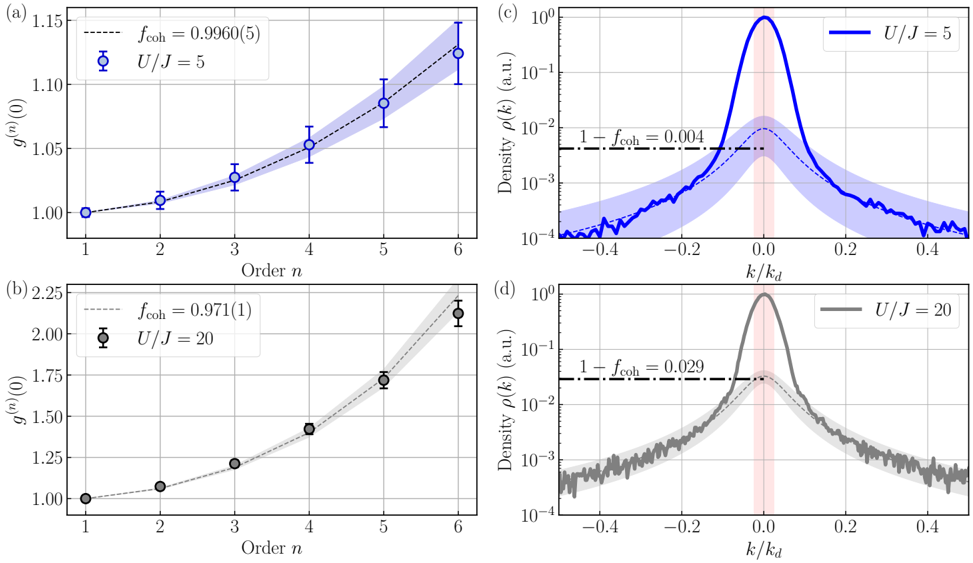COHERENT FRACTION OF BOSE SUPERFLUIDS IN THE BEC MODE At thermal equilibrium, a fraction of the total atom number is expelled from the BEC by the finite interactions (quantum depletion) and by the finite temperature FIG. 3. (a) -(b) Plots of g ( n ) (0) measured at k = 0 in lattice superfluids with U/J = 5 and U/J = 20. The data in panel (a) is identical to that of shown in Fig. 1(c). The dashed lines ( resp. the shaded areas) are the predictions of the model with the values f coh ( resp. the uncertainties on f coh ) fitted to the data. (c) -(d) Plots of 1D cuts through the momentum densities measured at U/J = 5 and U/J = 20 and normalized to their value at k = 0. The vertical shaded area indicates the volume occupied by the sphere S Ω where the counting statistics is evaluated. The horizontal dashed-dotted lines indicate the fitted values 1 -f coh . The dashed lines are Lorentzian functions fitted to the tails of the densities in the range [0 . 2 k d , 0 . 5 k d ] in order to estimate the density of the depletion at k = 0 (the shaded areas represent the error from the fitted parameters). <details> <summary>Image 3 Details</summary>  ### Visual Description \n ## Charts: Correlation Function and Density Distribution ### Overview The image presents four charts: (a) and (b) depict correlation functions, while (c) and (d) show density distributions. Charts (a) and (c) correspond to U/J = 5, and charts (b) and (d) correspond to U/J = 20. The correlation functions show the average value of a quantity (denoted as ⟨n(r)⟩) as a function of order 'n'. The density distributions show the probability density function ρ(k) as a function of k/kd. ### Components/Axes * **Charts (a) & (b):** * X-axis: Order n (ranging from approximately 1 to 6). * Y-axis: ⟨n(r)⟩ (ranging from approximately 1.0 to 2.25). * Data points: Represented by circles with error bars. * Shaded region: Represents the uncertainty around the fitted curve. * Text: "fcoh = 0.9960(5)" for (a) and "fcoh = 0.971(1)" for (b). * Label: "U/J = 5" for (a) and "U/J = 20" for (b). * **Charts (c) & (d):** * X-axis: k/kd (ranging from approximately -0.4 to 0.4, on a logarithmic scale). * Y-axis: Density ρ(k) (a.u.) (ranging from approximately 10^-4 to 10^0, on a logarithmic scale). * Lines: Represent the density distribution. * Shaded region: Represents the uncertainty or variation in the density distribution. * Text: "1 + fcoh = 0.004" for (c) and "1 + fcoh = 0.029" for (d). * Label: "U/J = 5" for (c) and "U/J = 20" for (d). * Red shaded region: Highlighted area around k/kd = 0. * **Legend (top-right):** * U/J = 5 (Blue line) * U/J = 20 (Black line) ### Detailed Analysis or Content Details * **Chart (a):** The blue line representing U/J = 5 shows an upward trend. * n = 1: ⟨n(r)⟩ ≈ 1.00, error bar ≈ ± 0.02 * n = 2: ⟨n(r)⟩ ≈ 1.04, error bar ≈ ± 0.02 * n = 3: ⟨n(r)⟩ ≈ 1.08, error bar ≈ ± 0.02 * n = 4: ⟨n(r)⟩ ≈ 1.12, error bar ≈ ± 0.03 * n = 5: ⟨n(r)⟩ ≈ 1.16, error bar ≈ ± 0.03 * n = 6: ⟨n(r)⟩ ≈ 1.20, error bar ≈ ± 0.04 * **Chart (b):** The black line representing U/J = 20 shows a steeper upward trend. * n = 1: ⟨n(r)⟩ ≈ 1.00, error bar ≈ ± 0.03 * n = 2: ⟨n(r)⟩ ≈ 1.20, error bar ≈ ± 0.04 * n = 3: ⟨n(r)⟩ ≈ 1.40, error bar ≈ ± 0.05 * n = 4: ⟨n(r)⟩ ≈ 1.60, error bar ≈ ± 0.06 * n = 5: ⟨n(r)⟩ ≈ 1.80, error bar ≈ ± 0.07 * n = 6: ⟨n(r)⟩ ≈ 2.00, error bar ≈ ± 0.08 * **Chart (c):** The blue line representing U/J = 5 shows a peak around k/kd = 0, with a relatively narrow distribution. * Peak density ≈ 1.0 * Density at k/kd = ±0.2 ≈ 0.1 * Density at k/kd = ±0.4 ≈ 0.01 * **Chart (d):** The black line representing U/J = 20 shows a broader peak around k/kd = 0, with a wider distribution. * Peak density ≈ 1.0 * Density at k/kd = ±0.2 ≈ 0.2 * Density at k/kd = ±0.4 ≈ 0.05 ### Key Observations * The correlation function ⟨n(r)⟩ increases with order 'n' for both U/J values, indicating a positive correlation. * The rate of increase in ⟨n(r)⟩ is significantly higher for U/J = 20 (Chart b) compared to U/J = 5 (Chart a). * The density distribution for U/J = 5 (Chart c) is more sharply peaked around k/kd = 0, suggesting a more localized distribution. * The density distribution for U/J = 20 (Chart d) is broader, indicating a more delocalized distribution. * The value of fcoh is higher for U/J = 5 (0.9960(5)) than for U/J = 20 (0.971(1)). ### Interpretation These charts likely represent the behavior of a system (possibly a quantum system) with different interaction strengths (U/J). The correlation function ⟨n(r)⟩ measures the spatial correlation of a quantity 'n' at different distances (represented by 'n'). The density distribution ρ(k) represents the distribution of the system in momentum space. The higher U/J value (20) leads to a faster increase in the correlation function, suggesting stronger correlations at larger distances. This could indicate a tendency towards ordering or localization. The broader density distribution for U/J = 20 supports this interpretation, as it implies that the system's momentum is more spread out, consistent with a more delocalized state. The fcoh parameter likely represents a coherence factor. The higher value for U/J = 5 suggests a higher degree of coherence in the system at that interaction strength. The red shaded region around k/kd = 0 in both density distribution charts may highlight a specific region of interest, potentially related to the system's ground state or a dominant scattering process. The logarithmic scale on the y-axis of the density distribution charts emphasizes the relative probabilities of different momentum values. </details> (thermal depletion). Even if it amounts to a negligible fraction of the atom number N Ω falling in S Ω , the total depletion of the condensate may contribute to the measured statistics. We define the 'coherent fraction' f coh as the fraction of N Ω that belongs to the BEC. Building on these considerations, we introduce a heuristic model that assumes (i) that atoms in the BEC and in the depletion contribute independently to the measured counting statistics in S Ω [44], and (ii) that the BEC is a coherent state while both the thermal and quantum depletion exhibit thermal statistics in S Ω . While a thermal FCS is expected for the thermal depletion, we emphasize that describing the contribution of the quantum depletion with a thermal statistics is an assumption. The statistics of the quantum depletion was shown to be thermal when measured at non-zero momenta, outside the BEC [35]. Whether this is also valid for small momenta within the BEC mode is difficult to assess in a harmonic trap. Finally, there is a priori no reason for our model to be valid in the strongly-interacting regime. In contrast to the weakly-interacting regime where the Bogoliubov approximation holds, neglecting the correlations between the condensate and its depletion at large interaction strengths could be an erroneous assumption. Our measurements however show that the model agrees with the experimental data over a wide range of interaction strengths. With the hypotheses of our model, we obtain an analytical prediction for g ( n ) (0) that depends only on the coherent fraction f coh (see Appendix E), $$g ^ { ( n ) } ( 0 ) - 1 = \sum _ { p = 1 } ^ { n - 1 } \left [ ( n - p ) ! \binom { n } { p } ^ { 2 } - \binom { n } { p } \right ] f _ { c o h } ^ { p } ( 1 - f _ { c o h } ) ^ { n - p } <text><loc_434><loc_205><loc_499><loc_255>(3) While</text> </doctag>$$ While our model straightforwardly predicts the magnitudes g ( n ) (0), this is not the case for the probability distribution P ( N Ω ). The latter results from a complex convolution of the probability distributions of the condensate and of the depletion and it is well established that obtaining P ( X ) from the moments of a random variable X is a difficult problem [52]. In Fig. 3(a), we fit the experimental data shown in Fig. 1(b) with the analytical prediction of Eq. (3), finding a good agreement with the coherent fraction as the only adjustable parameter (found equal to f c = 0 . 9960(5) for the case of U/J = 5). We then repeated our measurements for various condensate fractions. To do so, we change the lattice depth to obtain ratios of on-site interaction U to tunnelling amplitude J ranging from U/J = 2 to U/J = 22. In this range of parameters, the gas remains far from entering the Mott insulator regime expected at the critical ratio ( U/J ) c 25 -30 [49], but it enters the strongly-interacting regime where the condensate is strongly depleted (at U/J = 22 the condensate fraction is f c ∼ 0 . 15). In Fig. 3(b) we plot the magnitude of the n -body correlations for a lattice superfluids with an increased interaction U/J = 20. The deviation from the ideal coherent state is increased, in qualitative agreement with the physical picture at the root of the model. To be quantitative, we fit the experimental data with the analytical prediction of Eq. (3). Firstly, we confirm that Eq. (3) correctly fits the values of g ( n ) (0) with a single adjustable parameter f coh . Secondly, the extracted values of f coh decrease with the interaction strength as intuitively expected. The uncertainty on the values f coh is extremely small, at the ∼ 0 . 1% level. As can be inferred from Fig. 3, the larger the order n of correlations we measure, the smaller the uncertainty on f coh . This illustrates the extreme sensitivity of high-order correlations to probe many-body coherence. A quantitative test of the model would compare the value 1 -f coh to the fraction η D of depleted atoms detected within S Ω . We are not aware of a quantitative analytical prediction for η D in 3D interacting trapped lattice Bose gases. However, an indirect comparison is amenable from measuring the momentum densities. In Fig 3(c)-(d), we plot 1D cuts through the momentum densities measured at U/J = 5 and U/J = 20 and we fit the tails (in the range [0 . 2 k d , 0 . 5 k d ]) with a Lorentzian function to extrapolate the density of the depletion at k = 0. Using a Lorentzian function is an arbitrary choice which happens to correctly fit the tails. This analysis indicates that the values 1 -f coh are compatible with the extrapolated densities, while both quantities vary by one order of magnitude. 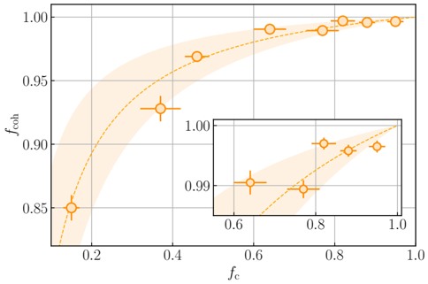To assess the validity of the model, we proceed with a quantitative comparison of the measured coherent fraction to the measured condensate fraction [47]. The coherent fraction f coh in S Ω differs from the condensate fraction f c of the entire gas since the radius of S Ω is much smaller than 2 π/L . Moreover, the scaling of f coh with f c is non-linear since f coh reveals the BEC atom number in a small volume S Ω where the BEC contribution is maximum while that of the depletion is small (except when f c 1). The volumes occupied by the BEC ( V c ) and by the depletion ( V d ) set their respective contributions in S Ω . A simple estimate (see Appendix F) leads to $$f _ { c o h } \simeq \frac { f _ { c } } { f _ { c } + ( 1 - f _ { c } ) \mathcal { V } _ { c } / \mathcal { V } _ { d } } . \quad \ \ ( 4 )$$ In Fig. 4 we plot the measured values of f coh and f c , along with the prediction of Eq. (4). Here, f c is obtained similarly to [47] and the ratio V c / V d used to plot Eq. (4) is estimated from the measured density pro- FIG. 4. Coherent fraction f coh as a function of the condensate fraction f c . The dashed-line is the prediction of Eq. (4) where the ratio V c / V d = 0 . 03(1) is evaluated from the measured density profiles (see Appendix F). The shaded area reflects the uncertainty on V c / V d . <details> <summary>Image 4 Details</summary>  ### Visual Description \n ## Chart: Coherence Factor vs. Correction Factor ### Overview The image presents a scatter plot with a fitted curve, illustrating the relationship between a coherence factor (`f_coh`) and a correction factor (`f_c`). The plot includes a shaded region representing uncertainty or variance around the fitted curve. A zoomed-in inset plot provides a more detailed view of the data in the upper-right quadrant of the main plot. ### Components/Axes * **X-axis:** Labeled `f_c` (Correction Factor). Scale ranges from approximately 0.0 to 1.0, with tick marks at 0.2, 0.4, 0.6, 0.8, and 1.0. * **Y-axis:** Labeled `f_coh` (Coherence Factor). Scale ranges from approximately 0.8 to 1.0, with tick marks at 0.85, 0.90, 0.95, and 1.00. * **Data Points:** Represented by orange circles with error bars. * **Fitted Curve:** A dashed orange line that approximates the trend of the data points. * **Uncertainty Region:** A light orange shaded area surrounding the fitted curve, indicating the range of possible values. * **Inset Plot:** A smaller plot positioned in the top-right corner, providing a zoomed-in view of the data between `f_c` values of 0.6 and 1.0. The inset plot has the same axes labels and visual elements as the main plot. ### Detailed Analysis The main plot shows a generally increasing trend between `f_c` and `f_coh`. As `f_c` increases, `f_coh` also tends to increase, but the rate of increase diminishes as `f_c` approaches 1.0. Here's a breakdown of approximate data points extracted from the main plot: * `f_c` ≈ 0.05, `f_coh` ≈ 0.85 (with error bar extending to approximately 0.80) * `f_c` ≈ 0.2, `f_coh` ≈ 0.90 (with error bar extending to approximately 0.85) * `f_c` ≈ 0.4, `f_coh` ≈ 0.95 (with error bar extending to approximately 0.90) * `f_c` ≈ 0.6, `f_coh` ≈ 0.97 (with error bar extending to approximately 0.92) * `f_c` ≈ 0.8, `f_coh` ≈ 0.99 (with error bar extending to approximately 0.97) * `f_c` ≈ 1.0, `f_coh` ≈ 1.00 (with error bar extending to approximately 0.98) The inset plot shows a similar trend, but with more detail in the region where `f_c` is close to 1.0. * `f_c` ≈ 0.65, `f_coh` ≈ 0.992 (with error bar extending to approximately 0.985) * `f_c` ≈ 0.8, `f_coh` ≈ 0.996 (with error bar extending to approximately 0.990) * `f_c` ≈ 0.9, `f_coh` ≈ 0.998 (with error bar extending to approximately 0.993) * `f_c` ≈ 1.0, `f_coh` ≈ 1.00 (with error bar extending to approximately 0.995) ### Key Observations * The relationship between `f_c` and `f_coh` appears to be non-linear, exhibiting diminishing returns as `f_c` increases. * The error bars indicate a degree of uncertainty in the data, particularly at lower values of `f_c`. * The inset plot suggests that the increase in `f_coh` slows down significantly as `f_c` approaches 1.0. * The fitted curve provides a smoothed representation of the underlying trend, but it's important to consider the uncertainty represented by the shaded region. ### Interpretation The chart likely represents a model or empirical observation where a correction factor (`f_c`) is applied to improve the coherence (`f_coh`) of a system or process. The diminishing returns observed as `f_c` approaches 1.0 suggest that there's a limit to the improvement that can be achieved through this correction. The error bars indicate that the relationship is not perfectly deterministic, and there's inherent variability in the system. The inset plot is included to highlight the behavior of the system when the correction factor is already relatively high. This could be important for understanding the practical limitations of the correction method. The data suggests that further increases in `f_c` beyond a certain point yield only marginal improvements in `f_coh`. The chart could be used to optimize the value of `f_c` to achieve a desired level of coherence, balancing the benefits of correction with the potential costs or limitations. The shaded region around the fitted curve is crucial for risk assessment and decision-making, as it provides a range of plausible outcomes. </details> files (see Appendix F). The quantitative prediction of our model (without any adjustable parameter) correctly reproduces the observed non-linear dependency of f coh with f c . As discussed previously, the agreement in the strongly-interacting regime is rather surprising. Understanding this fact requires a more elaborate theoretical approach than the one presented in this work. We observe that the heuristic model quantitatively captures the deviations to g ( n ) (0) = 1, attributing the latter to the presence of depleted atoms (both from the thermal and the quantum depletion). In turn, this suggests that BEC atoms have the statistics of a fully coherent state, with g ( n ) (0) = 1 at any order n ≤ 6. The role of the depletion in the many-body coherence unveiled in this work was not identified previously [33]. A major difference of our experiment with respect to that of [33] is that the volume V Ω used in that work to compute the statistics is larger than the coherence volume (2 π/L ) 3 , a choice made in light of a smaller detection efficiency η ∼ 0 . 08. Using too large of a volume V Ω entails a convolution of the correlation functions that significantly reduces their amplitudes and, in turn, hides the contribution from the depletion. This is illustrated by the fact that in the thermal case the authors of [33] find g (2) (0) = 1 . 022(2) and g (3) (0) = 1 . 061(6) instead of g (2) (0) = 2 and g (3) (0) = 6 . We conclude that our ability to obtain sufficient statistics in tiny volumes is a major asset to quantitatively probe many-body correlations. ## V. CONCLUSION We have presented measurements of the full counting statistics (FCS) and of perfectly-contrasted n -body correlations in interacting lattice Bose gases. We find that a Mott insulator exhibits a thermal statistics in the mo- mentum space with g ( n ) (0) = n !, while the condensate component is fully coherent with g ( n ) (0) = 1 (at least) up to n = 6. The latter conclusion derives from assuming that the heuristic model we introduce to analyse the FCS in Bose superfluids and to describe the contribution from the depletion of the condensate is valid. We have assessed this validity in the experiment from studying the coherent fraction at increasing interaction strengths. A theoretical validation is beyond the scope of this work. Our results represent the most stringent certifications of the many-body coherence properties of Mott insulators and of BECs, and they validate emblematic pure-state descriptions of n -body coherence up to the order n = 6. In the future, the experimental approach we use is readily extendable to probe the many-body coherence in a large variety of interacting quantum states and phase transitions realized on cold-atom platforms ( e.g. [911, 53]). It relies on (i) a free-fall expansion from the trap and (ii) a single-atom-resolved detection method. The first condition is ensured with lattice or low-dimensional (1D and 2D) gases for which interactions do not affect the expansion, as well as with quantum gases for which interactions are switched off during the expansion [54]. The second condition is met with various detection methods and atomic species [55]. - [1] Y. Blanter and M. B¨ uttiker, Shot noise in mesoscopic conductors, Physics Reports 336 , 1 (2000). - [2] C. Gardiner and P. Zoller, Quantum Noise - A Handbook of Markovian and Non-Markovian Quantum Stochastic Methods with Applications to Quantum Optics (Springer Berlin, Heidelberg, 2004). - [3] E. A. Burt, R. W. Ghrist, C. J. Myatt, M. J. Holland, E. A. Cornell, and C. E. Wieman, Coherence, correlations, and collisions: What one learns about bose-einstein condensates from their decay, Phys. Rev. Lett. 79 , 337 (1997). - [4] E. Altman, E. Demler, and M. D. Lukin, Probing manybody states of ultracold atoms via noise correlations, Phys. Rev. A 70 , 013603 (2004). - [5] T. Schweigler, V. Kasper, S. Erne, I. Mazets, B. Rauer, F. Cataldini, T. Langen, T. Gasenzer, J. Berges, and J. Schmiedmayer, Experimental characterization of a quantum many-body system via higher-order correlations, Nature 545 , 323 (2017). - [6] L. S. Levitov, H. Lee, and G. B. Lesovik, Electron counting statistics and coherent states of electric current, Journal of Mathematical Physics 37 , 4845 (1996). - [7] D. A. Ivanov and A. G. Abanov, Phase transitions in full counting statistics for periodic pumping, EPL (Europhysics Letters) 92 , 37008 (2010). - [8] F. J. G´ omez-Ruiz, J. J. Mayo, and A. del Campo, Full counting statistics of topological defects after crossing a phase transition, Phys. Rev. Lett. 124 , 240602 (2020). - [9] P. Devillard, D. Chevallier, P. Vignolo, and M. Albert, Full counting statistics of the momentum occupation numbers of the tonks-girardeau gas, Phys. Rev. A 101 , 063604 (2020). Another interesting direction consists in realizing recent proposals to access non-trivial n -body correlations [26, 27]. These theoretical works have shown that nondiagonal correlators can be accessed from combining twoparticle unitary transformations e.g. beamsplitters with a measurement of the FCS. Such protocols have many potential applications, from quantifying entanglement to implementing variational algorithms. ## ACKNOWLEDGEMENT We thank S. Butera, A. Browaeys, I. Carusotto, T. Lahaye, T. Roscilde and the members of the Quantum Gas group at Institut d'Optique for insightful discussions. We acknowledge financial support from the R´ egion Ile-de-France in the framework of the DIM SIRTEQ, the 'Fondation d'entreprise iXcore pour la Recherche', the Agence Nationale pour la Recherche (Grant number ANR-17-CE30-0020-01). D.C. acknowledges support from the Institut Universitaire de France. A. A. acknowledges support from the Simons Foundation and from Nokia-Bell labs. - [10] V. Eisler, Universality in the full counting statistics of trapped fermions, Phys. Rev. Lett. 111 , 080402 (2013). - [11] I. Lovas, B. D´ ora, E. Demler, and G. Zar´ and, Full counting statistics of time-of-flight images, Phys. Rev. A 95 , 053621 (2017). - [12] I. Klich and L. Levitov, Quantum noise as an entanglement meter, Phys. Rev. Lett. 102 , 100502 (2009). - [13] M. Esposito, U. Harbola, and S. Mukamel, Nonequilibrium fluctuations, fluctuation theorems, and counting statistics in quantum systems, Rev. Mod. Phys. 81 , 1665 (2009). - [14] S. Gustavsson, R. Leturcq, B. Simoviˇ c, R. Schleser, T. Ihn, P. Studerus, K. Ensslin, D. C. Driscoll, and A. C. Gossard, Counting statistics of single electron transport in a quantum dot, Phys. Rev. Lett. 96 , 076605 (2006). - [15] V. F. Maisi, D. Kambly, C. Flindt, and J. P. Pekola, Full counting statistics of andreev tunneling, Phys. Rev. Lett. 112 , 036801 (2014). - [16] T. C. Liebisch, A. Reinhard, P. R. Berman, and G. Raithel, Atom counting statistics in ensembles of interacting rydberg atoms, Phys. Rev. Lett. 95 , 253002 (2005). - [17] N. Malossi, M. M. Valado, S. Scotto, P. Huillery, P. Pillet, D. Ciampini, E. Arimondo, and O. Morsch, Full counting statistics and phase diagram of a dissipative rydberg gas, Phys. Rev. Lett. 113 , 023006 (2014). - [18] J. Zeiher, R. van Bijnen, P. Schauß, S. Hild, J.-y. Choi, T. Pohl, I. Bloch, and C. Gross, Many-body interferometry of a rydberg-dressed spin lattice, Nature Physics 12 , 1095 (2016). - [19] A. ¨ Ottl, S. Ritter, M. K¨ ohl, and T. Esslinger, Correlations and counting statistics of an atom laser, Phys. Rev. Lett. 95 , 090404 (2005). - [20] M. Perrier, Z. Amodjee, P. Dussarrat, A. Dareau, A. Aspect, M. Cheneau, D. Boiron, and C. I. Westbrook, Thermal counting statistics in an atomic two-mode squeezed vacuum state, SciPost Phys. 7 , 2 (2019). - [21] S. T. Flammia, D. Gross, Y.-K. Liu, and J. Eisert, Quantum tomography via compressed sensing: error bounds, sample complexity and efficient estimators, New Journal of Physics 14 , 095022 (2012). - [22] R. J. Glauber, The quantum theory of optical coherence, Phys. Rev. 130 , 2529 (1963). - [23] P. E. Dolgirev, J. Marino, D. Sels, and E. Demler, Nongaussian correlations imprinted by local dephasing in fermionic wires, Phys. Rev. B 102 , 100301 (2020). - [24] C. Fabre and N. Treps, Modes and states in quantum optics, Rev. Mod. Phys. 92 , 035005 (2020). - [25] M. Walschaers, Non-gaussian quantum states and where to find them, PRX Quantum 2 , 030204 (2021). - [26] E. Brunner, A. Buchleitner, and G. Dufour, Many-body coherence and entanglement from randomized correlation measurements, arXiv 10.48550/arxiv.2107.01686 (2021). - [27] P. Naldesi, A. Elben, A. Minguzzi, D. Cl´ ement, P. Zoller, and B. Vermersch, Fermionic correlation functions from randomized measurements in programmable atomic quantum devices, arXiv 10.48550/arxiv.2205.00981 (2022). - [28] A. Aspect, Hanbury brown and twiss, hong ou and mandel effects and other landmarks in quantum optics: from photons to atoms, in Current Trends in Atomic Physics , edited by A. Browaeys, T. Lahaye, T. Porto, C. S. Adams, M. Weidem¨ uller, and L. F. Cugliandolo (Oxford University Press, 2019). - [29] M. Schellekens, R. Hoppeler, A. Perrin, J. V. Gomes, D. Boiron, A. Aspect, and C. I. Westbrook, Hanbury brown twiss effect for ultracold quantum gases, Science 310 , 648 (2005). - [30] R. G. Dall, A. G. Manning, S. S. Hodgman, W. RuGway, K. V. Kheruntsyan, and A. G. Truscott, Ideal n-body correlations with massive particles, Nature Physics 9 , 341 (2013). - [31] T. Jeltes, J. M. McNamara, W. Hogervorst, W. Vassen, V. Krachmalnicoff, M. Schellekens, A. Perrin, H. Chang, D. Boiron, A. Aspect, and C. I. Westbrook, Comparison of the hanbury brown-twiss effect for bosons and fermions, Nature 445 , 402 (2007). - [32] A. Bergschneider, V. M. Klinkhamer, J. H. Becher, R. Klemt, L. Palm, G. Z¨ urn, S. Jochim, and P. M. Preiss, Experimental characterization of two-particle entanglement through position and momentum correlations, Nature Physics 15 , 640 (2019). - [33] S. S. Hodgman, R. G. Dall, A. G. Manning, K. G. H. Baldwin, and A. G. Truscott, Direct measurement of long-range third-order coherence in bose-einstein condensates, Science 331 , 1046 (2011). - [34] C. Carcy, H. Cayla, A. Tenart, A. Aspect, M. Mancini, and D. Cl´ ement, Momentum-space atom correlations in a mott insulator, Phys. Rev. X 9 , 041028 (2019). - [35] H. Cayla, S. Butera, C. Carcy, A. Tenart, G. Herc´ e, M. Mancini, A. Aspect, I. Carusotto, and D. Cl´ ement, Hanbury brown and twiss bunching of phonons and of the quantum depletion in an interacting bose gas, Phys. Rev. Lett. 125 , 165301 (2020). - [36] A. Tenart, G. Herc´ e, J.-P. Bureik, A. Dareau, and D. Cl´ ement, Observation of pairs of atoms at opposite momenta in an equilibrium interacting bose gas, Nature Physics 17 , 1364 (2021). - [37] M. Holten, L. Bayha, K. Subramanian, S. Brandstetter, C. Heintze, P. Lunt, P. M. Preiss, and S. Jochim, Observation of cooper pairs in a mesoscopic two-dimensional fermi gas, Nature 606 , 287 (2022). - [38] L. Mandel and E. Wolf, Optical Coherence and Quantum Optics (Cambridge University Press, 1995). - [39] L. P. Pitaevskii and S. Stringari, Bose-Einstein Condensation (Clarendon press, Oxford, 2004). - [40] S. F¨ olling, F. Gerbier, A. Widera, O. Mandel, T. Gericke, and I. Bloch, Spatial quantum noise interferometry in expanding ultracold atom clouds, Nature 434 , 481 (2005). - [41] E. Toth, A. M. Rey, and P. B. Blakie, Theory of correlations between ultracold bosons released from an optical lattice, Phys. Rev. A 78 , 013627 (2008). - [42] D. F. Walls and G. J. Milburn, Quantum Optics (Springer Berlin, Heidelberg, 2008). - [43] M. A. Kristensen, M. B. Christensen, M. Gajdacz, M. Iglicki, K. Paw lowski, C. Klempt, J. F. Sherson, K. Rza˙ zewski, A. J. Hilliard, and J. J. Arlt, Observation of atom number fluctuations in a bose-einstein condensate, Phys. Rev. Lett. 122 , 163601 (2019). - [44] Y. Castin and R. Dum, Low-temperature bose-einstein condensates in time-dependent traps: Beyond the u (1) symmetry-breaking approach, Phys. Rev. A 57 , 3008 (1998). - [45] Note that in the experiment the total atom number N is not strictly constant from shot to shot. However, the measurement of the FCS in a tiny volume V Ω is largely immune to small shot-to-shot fluctuations of N . - [46] J. Stenger, S. Inouye, A. P. Chikkatur, D. M. StamperKurn, D. E. Pritchard, and W. Ketterle, Bragg spectroscopy of a bose-einstein condensate, Phys. Rev. Lett. 82 , 4569 (1999). - [47] H. Cayla, C. Carcy, Q. Bouton, R. Chang, G. Carleo, M. Mancini, and D. Cl´ ement, Single-atom-resolved probing of lattice gases in momentum space, Phys. Rev. A 97 , 061609 (2018). - [48] A. Tenart, C. Carcy, H. Cayla, T. Bourdel, M. Mancini, and D. Cl´ ement, Two-body collisions in the time-of-flight dynamics of lattice bose superfluids, Phys. Rev. Research 2 , 013017 (2020). - [49] C. Carcy, G. Herc´ e, A. Tenart, T. Roscilde, and D. Cl´ ement, Certifying the adiabatic preparation of ultracold lattice bosons in the vicinity of the mott transition, Phys. Rev. Lett. 126 , 045301 (2021). - [50] K. Laiho, T. Dirmeier, M. Schmidt, S. Reitzenstein, and C. Marquardt, Measuring higher-order photon correlations of faint quantum light: A short review, Physics Letters A 435 , 128059 (2022). - [51] J. W. Goodman, Statistical optics , edited by W.-I. New York, Vol. 1 (1985). - [52] N. I. Akhiezer, The classical moment problem: and Some Related Questions in Analysis , edited by O. B. L. Edinburgh and London (1965). - [53] D. Contessi, A. Recati, and M. Rizzi, Phase diagram detection via gaussian fitting of number probability distribution, arXiv , 2207.01478 (2022). - [54] I. Bloch, J. Dalibard, and W. Zwerger, Many-body physics with ultracold gases, Rev. Mod. Phys. 80 , 885 (2008). - [55] H. Ott, Single atom detection in ultracold quantum gases: a review of current progress, Reports on Progress in Physics 79 , 054401 (2016). ## Appendix A. PROBABILITY DISTRIBUTION IN MOTT INSULATORS AND MULTIMODE THERMAL STATISTICS We consider the thermal statistics found in the case of Mott insulators. The bell-shaped correlation functions are well-fitted by a Gaussian function [34] and we introduce the two-body correlation length l c as $$g ^ { ( 2 ) } ( k _ { 1 } , k _ { 2 } ) = g ^ { ( 2 ) } ( 0 ) \times \exp \, \left ( \frac { - 2 | k _ { 1 } - k _ { 2 } \, | ^ { 2 } } { l _ { c } ^ { 2 } } \right ) . \quad ( 5 )$$ For the data set of a Mott insulator shown in the main text, the two-body correlation length is l c /k d = 0 . 031(2) and corresponds to the expected value [34], l c /k d ∼ 1 /N site where N site is the number of lattice sites occupied by the Mott insulator in the trap. In the case of a thermal statistics, the two-body correlation length in momentum space is equal to the inverse trap size of the gas, i.e. to the size of a mode in momentum space. We define a mode from its coherence volume V c as a cubic voxel of size 2 l c . When one computes two-body correlations in a cubic volume V Ω of size δk comparable to, or larger than, the correlation length l c , the measured magnitude differs from the fully-contrasted value g (2) (0) due to the spatial averaging of g (2) ( k 1 , k 2 ). For instance, using V Ω = V c , the magnitude of two-body correlations is reduced by a factor 1 / ( √ π/ 8 erf[ √ 2]) 3 ∼ 4 . 7. In contrast, we find that computing the probability distribution P ( N Ω ) is not affected by considering a volume V Ω ∼ V c , as we shall now discuss. In Fig. 5 we plot the probability distributions P ( N Ω ) computed with volumes V Ω equal or larger than V c . Firstly, we observe that the statistics is thermal when V Ω ≤ V c . More specifically, there is no need to ensure the condition V Ω V c to measure the probability distribution of a thermal statistics. Secondly, this statement is confirmed by analysing the measured probability distributions P ( N Ω ) for V Ω > V c . Indeed, the probability distribution computed over a number M of independent modes, each of which exhibiting a thermal statistics with an average occupation 〈 N 〉 , reads [20, 51] $$P _ { M } ( N _ { \Omega } ) = \frac { ( \langle N _ { \Omega } \rangle + M - 1 ) ! } { \langle N _ { \Omega } \rangle ! ( M - 1 ) ! } \frac { ( \langle N _ { \Omega } \rangle / M ) ^ { N _ { \Omega } } } { ( 1 + \langle N \rangle / M ) ^ { N _ { \Omega } + M } } .$$ In Fig. 5 the prediction P M ( N Ω ) for a multi-mode thermal statistics is plotted with a number of modes equal to M = V Ω /V c . These predictions are found to be in excellent agreement with the measured distributions without any adjustable parameters. 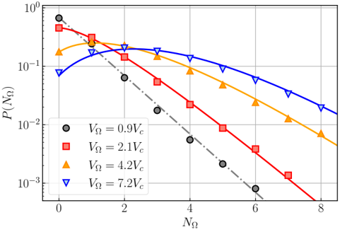FIG. 5. Probability distributions P ( N Ω ) measured in a Mott insulator with a varying voxel size V Ω . For V Ω = 0 . 9 V c , the measured distribution (black dots) matches the prediction (black dashed-dotted line) for a thermal distribution. For V Ω > V c , the measured distributions (red squares, orange triangles and blue triangles) agree with the predictions P M ( N Ω ) for a multi-mode thermal distribution (red, orange and blue solid lines). No adjustable parameters are used to plot the predictions P M ( N Ω ) that depend on the measured mean atom number 〈 N Ω 〉 and the chosen ratio M = V Ω /V c . <details> <summary>Image 5 Details</summary>  ### Visual Description ## Chart: Probability Distribution of NΩ ### Overview The image presents a chart illustrating the probability distribution P(NΩ) as a function of NΩ for different values of VΩ. The chart uses a logarithmic scale for the y-axis (P(NΩ)) and a linear scale for the x-axis (NΩ). Four distinct lines represent the probability distributions for VΩ values of 0.9V𝑐, 2.1V𝑐, 4.2V𝑐, and 7.2V𝑐. ### Components/Axes * **X-axis:** Labeled "NΩ", ranging from approximately 0 to 8. * **Y-axis:** Labeled "P(NΩ)", on a logarithmic scale, ranging from approximately 10⁻³ to 10⁰ (or 1). * **Legend:** Located in the bottom-left corner, listing the following data series: * Black circles: VΩ = 0.9V𝑐 * Red squares: VΩ = 2.1V𝑐 * Orange triangles: VΩ = 4.2V𝑐 * Blue triangles: VΩ = 7.2V𝑐 * **Grid:** A grid is present to aid in reading values from the chart. * **Vertical dashed line:** A vertical dashed line is present at approximately NΩ = 2. ### Detailed Analysis * **VΩ = 0.9V𝑐 (Black circles):** The line starts at approximately P(NΩ) = 0.9 at NΩ = 0, decreases rapidly, reaching approximately P(NΩ) = 0.01 at NΩ = 4, and continues to decrease, reaching approximately P(NΩ) = 0.001 at NΩ = 7. The trend is a steep downward slope. * **VΩ = 2.1V𝑐 (Red squares):** The line starts at approximately P(NΩ) = 0.2 at NΩ = 0, initially decreases, reaches a minimum around NΩ = 1.5 at approximately P(NΩ) = 0.08, then increases slightly before decreasing again. At NΩ = 8, P(NΩ) is approximately 0.01. The trend is initially decreasing, then slightly increasing, and finally decreasing. * **VΩ = 4.2V𝑐 (Orange triangles):** The line starts at approximately P(NΩ) = 0.1 at NΩ = 0, increases to a maximum around NΩ = 1.5 at approximately P(NΩ) = 0.15, then decreases. At NΩ = 8, P(NΩ) is approximately 0.03. The trend is increasing initially, then decreasing. * **VΩ = 7.2V𝑐 (Blue triangles):** The line starts at approximately P(NΩ) = 0.1 at NΩ = 0, increases to a maximum around NΩ = 2 at approximately P(NΩ) = 0.13, then decreases. At NΩ = 8, P(NΩ) is approximately 0.02. The trend is increasing initially, then decreasing. ### Key Observations * The probability distributions for all VΩ values decrease as NΩ increases, but the rate of decrease varies. * The distributions for VΩ = 4.2V𝑐 and VΩ = 7.2V𝑐 exhibit a peak before decreasing, suggesting a most probable value of NΩ around 1.5-2. * The distribution for VΩ = 0.9V𝑐 shows a monotonic decrease, indicating that higher values of NΩ are less probable. * The vertical dashed line at NΩ = 2 appears to mark a transition point where the distributions for VΩ = 4.2V𝑐 and VΩ = 7.2V𝑐 begin to decrease more rapidly. ### Interpretation The chart demonstrates how the probability distribution of NΩ changes with different values of VΩ. The parameter VΩ likely represents a potential or voltage, and NΩ could represent a related quantity, possibly the number of events or particles. The shape of the distributions suggests that the system's behavior is sensitive to the value of VΩ. The peak observed in the distributions for higher VΩ values indicates that there is a preferred value of NΩ for those conditions. As VΩ increases, the peak shifts slightly to the right, suggesting that the preferred value of NΩ also increases. The monotonic decrease for the lowest VΩ value suggests that the system is less likely to exhibit a preferred value of NΩ under those conditions. The vertical dashed line at NΩ = 2 might represent a threshold or critical point where the system's behavior changes significantly. The fact that the distributions for higher VΩ values start to decrease more rapidly after this point suggests that the system becomes less stable or more prone to fluctuations beyond this threshold. The logarithmic scale on the y-axis emphasizes the relative probabilities of different NΩ values. The steep slopes observed for some of the lines indicate that small changes in NΩ can lead to significant changes in probability. </details> ## Appendix B. MAGNITUDES OF CORRELATION FUNCTIONS IN MOTT INSULATORS ## A. Condition to measure fully-contrasted atom correlations As discussed in section II, obtaining fully-contrasted n -body correlation functions requires to probe the statistics in small voxels V Ω V c . This condition is much stringent than that ( V Ω ≤ V c ) to obtain the probability distribution P ( N Ω ). This poses serious difficulties in the case of a Mott insulator as its momentum-space density is low because a Mott insulator occupies a large volume in momentum-space, extending beyond the first Brillouin zone. The statistics of the atom number N Ω in a single voxel V Ω V c is therefore not sufficient to extract the magnitude g ( n ) (0) of the n -body correlation functions accurately, even when using an average over all the voxels contained in the first Brillouin zone. To circumvent this issue, we first compute the statistics in larger voxels from which the results in small voxels V Ω V c are then extrapolated. This procedure is detailed below. ## B. Magnitudes of correlation functions measured in voxels V Ω ∼ V c We first evaluate the magnitudes of correlation functions in anisotropic voxels of volume V ( δk ⊥ ) = δk × δk 2 ⊥ with δk ⊥ ≥ l c > δk = 0 . 015 k d . The volume V ( δk ⊥ ) ∼ V c is sufficiently large to compute the statistics of N δk ⊥ . To proceed, we divide the first Brillouin zone in voxels of volume V ( δk ⊥ ) and label each voxel with an integer j . The factorial moment in one voxel is denoted 〈 N δk ⊥ ( N δk ⊥ -1) ... ( N δk ⊥ -n + 1) 〉 j and the average of the factorial moments over the first Brillouin zone reads $$\sum _ { j } \, \langle N _ { \delta k _ { \perp } } ( N _ { \delta k _ { \perp } } - 1 ) \dots ( N _ { \delta k _ { \perp } } - n + 1 ) \rangle _ { j } . \quad ( 7 )$$ We obtain the magnitudes of correlation functions from normalizing the average value of the factorial moments, $$g _ { \delta k _ { \perp } } ^ { ( n ) } ( 0 ) = \frac { \sum _ { j } \, \langle N _ { \delta k _ { \perp } } ( N _ { \delta k _ { \perp } } - 1 ) \dots ( N _ { \delta k _ { \perp } } - n + 1 ) \rangle _ { j } } { \sum _ { j } \, \langle N _ { \delta k _ { \perp } } \rangle _ { j } ^ { n } } .$$ In the case of two-body correlations, an alternative to the approach based on the factorial moments is to compute the histogram of atom pairs [34]. We have verified that both approaches yield similar results for the magnitude g (2) δk ⊥ (0). ## C. Magnitudes of correlation functions measured in voxels V Ω V c We repeat the above analysis for voxels of varying volume, by changing the transverse size δk ⊥ , with the results plotted in Fig. 6. These results illustrate the fact that the magnitudes of the correlation functions are reduced when the voxel used to compute the statistics is too large, i.e. of the order or larger than the coherence volume V c . The fully-contrasted magnitude g ( n ) (0), expected in voxels V Ω V c , is the value of g ( n ) δk ⊥ (0) in the limit δk ⊥ → 0. We fit the measured variations of g ( n ) δk ⊥ (0) with δk ⊥ (see dashed-line in Fig. 6) and extrapolate g ( n ) (0) in the limit δk ⊥ → 0. ## Appendix C. PROBABILITY DISTRIBUTION AND MAGNITUDES OF CORRELATION FUNCTIONS IN BOSE SUPERFLUIDS The magnitudes of the normalized correlation functions are obtained from the factorial moments of the atom number N Ω in the small volume V Ω V c . In the case of the BEC mode at k = 0 , the average number of atoms in V Ω is relatively large, 〈 N Ω 〉 ∼ 5. As a consequence, the statistics in V Ω is sufficient to extract accurately the factorial moments. The n -factorial moment is defined as 〈 ( N Ω ) n 〉 = 〈 N Ω ( N Ω -1) ... 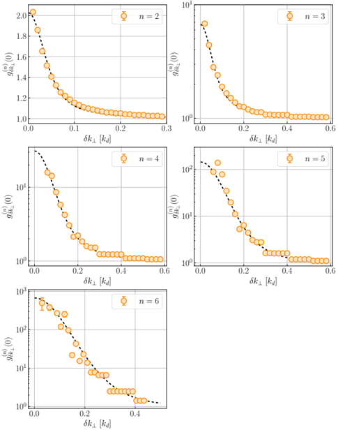( N Ω -n +1) 〉 and g ( n ) (0) are expressed as $$g ^ { ( n ) } ( 0 ) = \frac { \langle N _ { \Omega } ( N _ { \Omega } - 1 ) \dots ( N _ { \Omega } - n + 1 ) \rangle } { \langle N _ { \Omega } \rangle ^ { n } } = \frac { \langle ( N _ { \Omega } ) _ { n } \rangle } { \langle N _ { \Omega } \rangle ^ { n } } \quad t h e r ( 9 ) \quad s t a t i s$$ ⊥ FIG. 6. Plot of the magnitude g ( n ) δk ⊥ (0) as a function of the transverse integration δk ⊥ . The different panels correspond to different orders n of correlation functions, from n = 2 to n = 6. Apart from the data for n = 2 plotted in linear scale, the vertical axes are in log scale. <details> <summary>Image 6 Details</summary>  ### Visual Description ## Chart: Correlation Function Plots for Different 'n' Values ### Overview The image presents six individual plots, arranged in a 2x3 grid. Each plot displays a correlation function, g⁽ⁿ⁾(0), as a function of δk⊥/kᵈ. Each plot corresponds to a different value of 'n' (n=2, 3, 4, 5, 6), indicated at the top-right corner of each subplot. The plots appear to show a decay in the correlation function with increasing δk⊥/kᵈ. The y-axis is on a logarithmic scale for n=3, 4, 5, and 6. ### Components/Axes * **x-axis label (all plots):** δk⊥ [kᵈ] * **y-axis label (n=2):** g⁽²⁾(0) * **y-axis label (n=3, 4, 5, 6):** g⁽ⁿ⁾(0) (logarithmic scale) * **Title (each plot):** "n = [value]" where [value] is 2, 3, 4, 5, or 6. * **Data Series:** A single series of orange data points with error bars in each plot. * **Grid:** Each plot has a grid with lines at integer values on both axes. ### Detailed Analysis or Content Details **Plot 1: n = 2** * The data series shows a decreasing trend. * At δk⊥/kᵈ ≈ 0.0, g⁽²⁾(0) ≈ 1.9. * At δk⊥/kᵈ ≈ 0.1, g⁽²⁾(0) ≈ 1.4. * At δk⊥/kᵈ ≈ 0.2, g⁽²⁾(0) ≈ 1.1. * At δk⊥/kᵈ ≈ 0.3, g⁽²⁾(0) ≈ 1.0. **Plot 2: n = 3** * The data series shows a rapid initial decrease, followed by a slower decay. * At δk⊥/kᵈ ≈ 0.0, g⁽³⁾(0) ≈ 10¹. * At δk⊥/kᵈ ≈ 0.1, g⁽³⁾(0) ≈ 5. * At δk⊥/kᵈ ≈ 0.2, g⁽³⁾(0) ≈ 2. * At δk⊥/kᵈ ≈ 0.3, g⁽³⁾(0) ≈ 1.2. * At δk⊥/kᵈ ≈ 0.4, g⁽³⁾(0) ≈ 0.8. * At δk⊥/kᵈ ≈ 0.6, g⁽³⁾(0) ≈ 0.6. **Plot 3: n = 4** * Similar trend to n=3, with a rapid initial decrease. * At δk⊥/kᵈ ≈ 0.0, g⁽⁴⁾(0) ≈ 10². * At δk⊥/kᵈ ≈ 0.1, g⁽⁴⁾(0) ≈ 8. * At δk⊥/kᵈ ≈ 0.2, g⁽⁴⁾(0) ≈ 3. * At δk⊥/kᵈ ≈ 0.3, g⁽⁴⁾(0) ≈ 1.5. * At δk⊥/kᵈ ≈ 0.4, g⁽⁴⁾(0) ≈ 0.9. * At δk⊥/kᵈ ≈ 0.6, g⁽⁴⁾(0) ≈ 0.6. **Plot 4: n = 5** * Similar trend to n=4. * At δk⊥/kᵈ ≈ 0.0, g⁽⁵⁾(0) ≈ 10². * At δk⊥/kᵈ ≈ 0.1, g⁽⁵⁾(0) ≈ 7. * At δk⊥/kᵈ ≈ 0.2, g⁽⁵⁾(0) ≈ 2.5. * At δk⊥/kᵈ ≈ 0.3, g⁽⁵⁾(0) ≈ 1.2. * At δk⊥/kᵈ ≈ 0.4, g⁽⁵⁾(0) ≈ 0.8. * At δk⊥/kᵈ ≈ 0.6, g⁽⁵⁾(0) ≈ 0.6. **Plot 5: n = 6** * Similar trend to n=5. * At δk⊥/kᵈ ≈ 0.0, g⁽⁶⁾(0) ≈ 10³. * At δk⊥/kᵈ ≈ 0.1, g⁽⁶⁾(0) ≈ 10². * At δk⊥/kᵈ ≈ 0.2, g⁽⁶⁾(0) ≈ 4. * At δk⊥/kᵈ ≈ 0.3, g⁽⁶⁾(0) ≈ 1.8. * At δk⊥/kᵈ ≈ 0.4, g⁽⁶⁾(0) ≈ 0.9. ### Key Observations * The correlation function decreases as δk⊥/kᵈ increases for all values of 'n'. * The initial rate of decay is faster for higher values of 'n'. * The y-axis scale is logarithmic for n=3, 4, 5, and 6, indicating a wider range of correlation function values. * The error bars are relatively small, suggesting good precision in the measurements. ### Interpretation The plots demonstrate the decay of higher-order correlation functions with increasing wavevector difference (δk⊥). The parameter 'n' likely represents the order of the correlation function, and the plots show that higher-order correlations decay more rapidly. This suggests that the system becomes more disordered or uncorrelated as the wavevector difference increases, and this effect is more pronounced for higher-order correlations. The logarithmic scale used for n=3, 4, 5, and 6 indicates that these correlation functions span a much wider range of values than the second-order correlation function (n=2). The consistent decay pattern across different 'n' values suggests a fundamental property of the system being investigated. The data suggests a transition from correlated to uncorrelated behavior as δk⊥/kᵈ increases. The error bars indicate the uncertainty in the measurements, and their small size suggests a high degree of confidence in the observed trends. </details> We define the error bars on g ( n ) (0) as ∆( N Ω ) n / 〈 N Ω 〉 n , where ∆( N Ω ) n is the standard error of the factorial moment of order n , $$\Delta ( N _ { \Omega } ) _ { n } = \frac { 1 } { \sqrt { N _ { r u n s } } } \sqrt { \langle ( N _ { \Omega } ) _ { n } ^ { 2 } \rangle - \langle ( N _ { \Omega } ) _ { n } \rangle ^ { 2 } } \quad ( 1 0 )$$ ## Appendix D. RANDOMIZED DATA AND UPPER LIMIT OF THE ORDER OF CORRELATIONS We use the randomized data to estimate up to which order n we are able to compute the magnitudes of correlation functions correctly. As explained in the main text, the randomized data sets are built from the actual data sets of the experiment by shuffling the atoms from a given shot into many different shots. By construction, the randomized data has the same number of shots and of atoms per shot than the non-randomized data. Therefore we expect it to provide a means to test the accuracy of the finite data sets we use: because the randomized data should exhibit a perfect Poisson statistics, a systematic deviation to the latter is used as a signal of insufficient statistics. As illustrated in Fig. 7 in the case of Bose superfluids at U/J = 5 (same data set as the one shown in Fig. 1 of the main text), we are able to compute correlations of order larger than n = 6. However, for n > 6 we observe a systematic shift to the expected value g ( n ) (0) = 1 in the randomized data. We attribute this systematic shift to the fact that there are too few shots with an atom number N Ω > 6 to correctly evaluate the probability to find N Ω = n for n > 6. We therefore restrict our analysis to the orders n ≤ 6. A similar analysis for the other data sets shown in this work yields the same result. FIG. 7. Magnitude g ( n ) (0) as a function of the order n of correlations. The blue circles correspond to experimental data measured in Bose superfluids at U/J = 5. The orange squares correspond to the randomized data set. 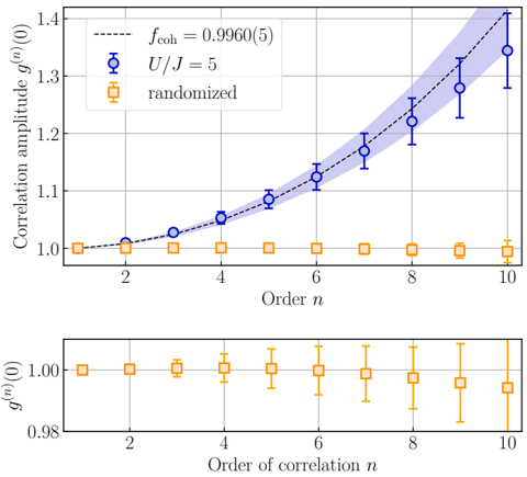<details> <summary>Image 7 Details</summary>  ### Visual Description ## Chart: Correlation Amplitude vs. Order ### Overview The image presents a chart comparing the correlation amplitude, g(n), as a function of the order 'n' for three different conditions: a coherent system (blue), a system with U/J = 5 (orange circles), and a randomized system (orange squares). The chart consists of two subplots, the top one showing the correlation amplitude for all three conditions, and the bottom one focusing on the randomized system with a zoomed-in y-axis. ### Components/Axes * **X-axis (both plots):** "Order n" or "Order of correlation n". Scale ranges from approximately 1 to 10, with tick marks at integer values. * **Y-axis (top plot):** "Correlation amplitude g(n)". Scale ranges from approximately 1.0 to 1.4, with tick marks at 0.2 intervals. * **Y-axis (bottom plot):** "g(n)". Scale ranges from approximately 0.98 to 1.02, with tick marks at 0.02 intervals. * **Legend (top-left):** * Blue line with error bars: "f_coh = 0.9960(5)" * Orange circles with error bars: "U/J = 5" * Orange squares with error bars: "randomized" * **Grid:** A light gray grid is present on both plots, aiding in data point localization. ### Detailed Analysis or Content Details **Top Plot:** * **Blue Line (f_coh = 0.9960(5)):** The blue line represents a coherent system. It exhibits a clear upward trend, indicating that the correlation amplitude increases with increasing order 'n'. * n = 1: g(n) ≈ 1.08 ± 0.03 * n = 2: g(n) ≈ 1.12 ± 0.03 * n = 3: g(n) ≈ 1.16 ± 0.03 * n = 4: g(n) ≈ 1.20 ± 0.03 * n = 5: g(n) ≈ 1.24 ± 0.03 * n = 6: g(n) ≈ 1.28 ± 0.03 * n = 7: g(n) ≈ 1.32 ± 0.03 * n = 8: g(n) ≈ 1.36 ± 0.03 * n = 9: g(n) ≈ 1.40 ± 0.03 * n = 10: g(n) ≈ 1.44 ± 0.03 * **Orange Circles (U/J = 5):** The orange circles represent a system with U/J = 5. The data points are relatively flat, fluctuating around g(n) ≈ 1.0. * n = 1: g(n) ≈ 1.03 ± 0.03 * n = 2: g(n) ≈ 1.01 ± 0.03 * n = 3: g(n) ≈ 1.02 ± 0.03 * n = 4: g(n) ≈ 1.03 ± 0.03 * n = 5: g(n) ≈ 1.01 ± 0.03 * n = 6: g(n) ≈ 1.01 ± 0.03 * n = 7: g(n) ≈ 1.02 ± 0.03 * n = 8: g(n) ≈ 1.01 ± 0.03 * n = 9: g(n) ≈ 1.02 ± 0.03 * n = 10: g(n) ≈ 1.00 ± 0.03 * **Orange Squares (randomized):** The orange squares represent a randomized system. The data points are also relatively flat, fluctuating around g(n) ≈ 1.0. * n = 1: g(n) ≈ 1.01 ± 0.03 * n = 2: g(n) ≈ 0.99 ± 0.03 * n = 3: g(n) ≈ 1.01 ± 0.03 * n = 4: g(n) ≈ 1.00 ± 0.03 * n = 5: g(n) ≈ 1.00 ± 0.03 * n = 6: g(n) ≈ 1.01 ± 0.03 * n = 7: g(n) ≈ 1.00 ± 0.03 * n = 8: g(n) ≈ 1.01 ± 0.03 * n = 9: g(n) ≈ 1.00 ± 0.03 * n = 10: g(n) ≈ 1.00 ± 0.03 **Bottom Plot:** * **Orange Squares (randomized):** This plot is a zoomed-in view of the randomized data from the top plot. The data points remain consistently around g(n) ≈ 1.0, with error bars indicating the uncertainty. ### Key Observations * The coherent system (blue line) exhibits a strong positive correlation between correlation amplitude and order 'n'. * Both the U/J = 5 system (orange circles) and the randomized system (orange squares) show minimal variation in correlation amplitude with respect to order 'n', remaining close to 1.0. * The error bars on all data points indicate a degree of uncertainty in the measurements. * The bottom plot confirms the flatness of the randomized system's correlation amplitude. ### Interpretation The data suggests that the coherent system demonstrates a long-range correlation, as evidenced by the increasing correlation amplitude with increasing order 'n'. This indicates that elements in the system are strongly linked, even over larger distances. In contrast, the U/J = 5 system and the randomized system lack this long-range correlation, as their correlation amplitudes remain close to 1.0, indicating a lack of significant correlation beyond immediate neighbors. The randomized system, by definition, should exhibit minimal correlation, and the data confirms this. The U/J = 5 system, while not fully coherent, shows a slight tendency towards correlation, but it is not statistically significant given the error bars. The value f_coh = 0.9960(5) likely represents a coherence factor for the coherent system, indicating a high degree of coherence. The error of (5) suggests the uncertainty in the coherence factor. The difference in behavior between the coherent system and the other two suggests that the coherence is a key factor in establishing long-range correlations within the system. </details> ## Appendix E. MODEL FOR THE MAGNITUDES OF CORRELATIONS IN BOSE SUPERFLUIDS We introduce a simple model to account for the presence of atoms belonging both to the BEC and to its depletion in the central voxel located at k = 0 . The depletion of the condensate results from the sum of the quantum depletion (induced by interactions) and the thermal depletion (induce by the finite temperature). As we have no mean to distinguish between the quantum and the thermal depletion, the depletion of the condensate we refer to in the following is the sum of both contributions. We assume that the statistical properties of the BEC mode are those of a coherent state, g ( n ) BEC (0) = 1. In contrast, the statistical properties of the depletion are assumed to be those of a thermal state, g ( n ) dep (0) = n !. This latter assumption holds because we consider a small voxel of size dk = 0 . 025 k d l c 0 . 15 k d where the correlation length l c is set by the inverse in-trap size 1 /L of the gas (see the main text). Moreover, we further assume that the BEC and depletion operators are uncorrelated. This is valid because the voxel we consider is much smaller than the volume occupied by the depletion, implying that the correlation between the total number of BEC atoms and the total number of depleted atoms (in the canonical ensemble) can be safely neglected. We are interested in the statistical properties of the atom number ˆ N Ω = a † Ω a Ω falling in the considered voxel, where a Ω = a BEC + a dep is the sum of the operators associated with the BEC and the depletion. Since we assume the operators a BEC and a dep are uncorrelated, one simply obtains $$\langle ( a _ { \Omega } ^ { \dagger } ) ^ { n } a _ { \Omega } ^ { n } \rangle = \sum _ { p = 1 } ^ { n } { n \choose p } ^ { 2 } \langle ( a _ { B E C } ^ { \dagger } ) ^ { p } a _ { B E C } ^ { p } ( a _ { d e p } ^ { \dagger } ) ^ { n - p } a _ { d e p } ^ { n - p } \rangle$$ where by definition a n Ω = ∑ n p =1 ( n p ) a p BEC a n -p dep . This leads to the formula given in the main text, $$g ^ { ( n ) } ( 0 ) - 1 & = \frac { \langle ( a _ { \Omega } ^ { \dagger } ) ^ { n } a _ { \Omega } ^ { n } \rangle } { \langle a _ { \Omega } ^ { \dagger } a _ { \Omega } \rangle ^ { n } } - 1 \\ & = \sum _ { p = 1 } ^ { n - 1 } \left [ ( n - p ) ! \binom { n } { p } ^ { 2 } - \binom { n } { p } \right ] f _ { c o h } ^ { p } ( 1 - f _ { c o h } ) ^ { n - p }$$ ## Appendix F. RELATION f coh VERSUS f c . The coherent fraction is approximatively given by $$f _ { c o h } \simeq \frac { \rho _ { B E C } ( 0 ) } { \rho _ { B E C } ( 0 ) + \rho _ { d e p } ( 0 ) } \quad \ \ ( 1 2 )$$ where ρ BEC (0) ( resp. ρ dep (0)) is the momentum density of the BEC ( resp. of the depletion) at the center of the Brillouin zone, k = 0. The condensate fraction is approximately given by $$f _ { c } \simeq \frac { \rho _ { B E C } ( 0 ) \mathcal { V } _ { c } } { \rho _ { B E C } ( 0 ) \mathcal { V } _ { c } + \rho _ { d e p } ( 0 ) \mathcal { V } _ { d } } \quad ( 1 3 )$$ where V c ( resp. V d ) is the total volume of the momentum-space occupied by the BEC ( resp. by the depletion) normalized to the density at k = 0. Combining these two definitions, one obtains the equation Eq. (4) of the main text. To compare the prediction of Eq. (4) with the measurements, we need to evaluate the volumes V c and V d . We describe the BEC density profile with an isotropic function [46] $$n _ { B E C } ( \mathbf k ) = \rho _ { B E C } ( 0 ) e ^ { - k ^ { 2 } / 2 \sigma _ { b e c } ^ { 2 } } \quad ( 1 4 ) \quad \begin{array} { l l } { { d e n } } \\ { { v / } } \end{array}$$ and the density profile of the depletion with a lorentzian function along each (uncoupled) lattice axis, $$n _ { d e p } ( k ) = \rho _ { d e p } ( 0 ) \, \Pi _ { j = x , y , z } \left ( \frac { \sigma _ { d e p } ^ { 2 } / 4 } { k _ { j } ^ { 2 } + ( \sigma _ { d e p } / 2 ) ^ { 2 } } \right ) . \quad ( 1 5 )$$ We obtain V c = ( √ 2 πσ bec ) 3 and V d = ( σ dep arctan [ k d σ dep ]) 3 . From fitting the measured density profiles with the above dependency, we obtain V c / V d = 0 . 03(1), a value which we use to plot the theoretical prediction in Fig. 4.