2207.14140v1

## Playing a 2D Game Indefinitely using NEAT and Reinforcement Learning Jerin Paul Selvan Dept. of Computer Engineering Pune Institute of Computer Technology Pune, India jerinsprograms@gmail.com Abstract -For over a decade now, robotics and the use of artificial agents have become a common thing. Testing the performance of new path finding or search space optimisation algorithms has also become a challenge as they require simulation or an environment to test them. The creation of artificial environments with artificial agents is one of the methods employed to test such algorithms. Games have also become an environment to test them. The performance of the algorithms can be compared by using artificial agents that will behave according to the algorithm in the environment they are put in. The performance parameters can be, how quickly the agent is able to differentiate between rewarding actions and hostile actions. This can be tested by placing the agent in an environment with different types of hurdles and the goal of the agent is to reach the farthest by taking decisions on actions that will lead to avoiding all the obstacles. The environment chosen is a game called 'Flappy Bird'. The goal of the game is to make the bird fly through a set of pipes of random heights. The bird must go in between these pipes and must not hit the top, the bottom, or the pipes themselves. The actions that the bird can take are either to flap its wings or drop down with gravity. The algorithms that are enforced on the artificial agents are NeuroEvolution of Augmenting Topologies (NEAT) and Reinforcement Learning. The NEAT algorithm takes an 'N' initial population of artificial agents. They follow genetic algorithms by considering an objective function, crossover, mutation, and augmenting topologies. Reinforcement learning, on the other hand, remembers the state, the action taken at that state, and the reward received for the action taken using a single agent and a Deep Q-learning Network. The performance of the NEAT algorithm improves as the initial population of the artificial agents is increased. Keywords -NeuroEvolution of Augmenting Topologies (NEAT), Artificial agent, Artificial environment, Game, Reinforcement Learning (RL) ## I. INTRODUCTION An intelligent agent is anything that can detect its surroundings, act independently to accomplish goals, and learn from experience or use knowledge to execute tasks better. The agent's surroundings are considered an environment in artificial intelligence. The agent uses actuators to send its output to the environment after receiving information from it through sensors. [11] There are several types of environments, Fully Observable vs Partially Observable, Deterministic vs Stochastic, Competitive vs Collaborative, Single-agent vs Multi-agent, Static vs Dynamic, Discrete vs Continuous, Dr. P. S. Game Dept. of Computer Engineering Pune Institute of Computer Technology Pune, India psgame@pict.edu Episodic vs Sequential and Known vs Unknown. An approach to machine learning known as NEAT, or Neuroevolution of Augmenting Topologies, functions similarly to evolution. In its most basic form, [1] NEAT is a technique for creating networks that are capable of performing a certain activity, like balancing a pole or operating a robot. It's significant that NEAT networks can learn using a reward function as opposed to back-propagation. By executing actions and observing the outcomes of those actions, an agent learns how to behave in a given environment via reinforcement learning, a feedbackbased machine learning technique. The agent receives compliments for each positive activity and is penalised or given negative feedback for each negative action. In contrast to supervised learning, reinforcement learning uses feedback to autonomously train the agent without the use of labelled data. The agent can only learn from its experience because there is no labelled data. In situations like gaming, robotics, and the like, where decisions must be made sequentially and with a long-term objective, RL provides a solution. The agent engages with the environment and independently explores it. In reinforcement learning, an agent's main objective is to maximise positive rewards while doing better. ## II. LITERATURE SURVEY Games have been used a lot to act as an environment to test algorithms. There is a lot of research [3] done to create an AI bot that can challenge a player in a multi-player or two-player game. Neuroevolution and Reinforcement learning algorithms are some of the algorithms that are used to create AI bots or artificial agents. [1], [7] and [8] have implemented a configuration of an ANN called Neuroevolution. The algorithm does not depend on the actions taken by the agents as a whole. [3], [4], [5], [6] and [7] use Reinforcement Learning algorithm with Deep Q-Learning to train the agents. The performance of the Neuroevolution algorithm depends on the objective function, initial population, mutation rate, weights and bias added to the network, the activation function used and overall topology of the network. Authors in [2] talk about how superior the Neuroevolution algorithm is over the traditional Reinforcement Learning algorithm with the Deep Q-Learning algorithm. Neuroevolution has an upper hand when it comes to the time taken by the artificial agent to train itself. There are other parameters that need to be taken into consideration while using a Neural Network. The topology of the network plays a vital role in the performance. Two strategies were proposed by Evgenia Papavasileiou (2021) [2], using fixed topologies in the neural networks and using augmented topologies. The network topology is a single hidden layer of neurons, with each hidden neuron connected to every network input and every network output. Evolution searches the space of connection weights of this fully-connected topology by allowing high performing networks to reproduce. The weight space is explored through the crossover of network weight vectors and through the mutation of single networks' weights. Thus, the goal of fixed-topology NE is to optimise the connection weights that determine the functionality of a network. The topology, or structure, of neural networks also affects their functionality, and modifying the network structure has been effective as part of supervised training. There are two ways of making use of the environment. Authors in [3], [4], [6] and [7] use DNN to extract the features from the frame of the game and they form the input to the agent. However, [1], [5] and [8] make use of the game itself and place the agent to perceive its surroundings. There are several combinations of Reinforcement Learning algorithms possible, like Deep Neural Networks (DNN), Long short-term memory (LSTM), Deep Q-Network (DQN) and the like. However, depending on the type of obstacle and the type of game, its performance varies. Reinforcement Learning algorithm with DNN and LSTM have been used in [3]. This algorithm addresses issues like vast search space, dependencies between the actions taken by the agent, the state and the environment, inputs and imperfect information. To reduce the complexity of the data generated by the perception of the agent, data skipping techniques are implemented. There is, however, a drawback with this algorithm. It takes a lot of time for the agent to train. Or, for every discrete step taken by the agent, it receives a state that belongs to a set S and it sends an action from the set A actions to the environment. The environment makes a transition from state St to St+1 and a gamma value [0, 1] determines the preference for immediate reward over longterm reward. A self-playing method is used by storing the parameters of the network to create a pool of past agents. This pool of past agents is used to sample opponents. This method offers RL to learn the Nash equilibrium strategy. Data skipping techniques were proposed in this paper. It refers to the process of dropping certain data during the training and evaluation process. Data skipping techniques proposed are: 'no-op' and 'maintain move decision'. The network is composed of an LSTM-based architecture, which has four heads with a shared state representation layer. An actor-critic off-policy learning algorithm was proposed. Botong Liu (2020) [4] has used Reinforcement Learning with DQN. The game was split into frames, and each game image was sequentially scaled, grayed, and adjusted for brightness. Deep Q Network algorithm was used to convert the game decision problem into a classification and recognition prob- lem of multi-dimensional images and solve it using CNN. Reinforcement learning works best for continuous decisionmaking problems. However, Deep Reinforcement Learning has a limitation of not converging for which Neural fitted Q-learning and DQN algorithms were used to overcome the issue. Since FNQ can work with numerical information only the author suggests use of DQN. Combining Q learning with CNN, the DQN can achieve self-learning. ReLu and maximum pooling layers are added to the CNN. Gradient descent (Adam Optimizer) was used to train the DQN parameters. Q-Value function based algorithms are the focus of Aidar Shakerimov (2021) [5]. For the DQN algorithms, improvements could be achieved in their performance by using a cumulative reward for training actions. To speed up training, RNN-ReLU was used instead of LSTM or GRU. LSTM or GRU performs better than RNN-ReLU but takes 7 times more time to train. Label smoothing was used to prevent the vanishing gradients in RNN-ReLU. However, DQN is sensitive to seed randomization. SARSA is a slight variation of the traditional Q-Learning algorithm. Authors in [6] use SARSA and Q-Learning algorithms with modifications such as -greedy policy, discretization and backward updates. Some variants of Q-Learning were also implemented such as a tabular approach, Q-value approximation using linear regression, and NN. In the implementation, [6] finds the SARSA algorithm to have outperformed Q-learning. The specifications of the rewards are a positive 5 for passing a pipe, a negative 1000 for hitting a pipe, and a positive 0.5 for surviving a frame. Feed-forward NN was used with a 3 neuron input layer, 50 neuron hidden layer, 20 neuron hyphen layer, and a 2 neuron output layer (ReLU activation function). The CNN is used with preprocessed input image by removing the background, grayscale, and resizing to 80 x 80, 2 CNN layers were used, one using sixteen 5 × 5 kernels with stride 2, and another with thirty-two 5 × 5 kernels with stride 2. [7] proposes the use of specific feature selection and presents the state by the bird velocity and the difference between the bird's position and the next lower pipe. This reduces the feature space and eliminates the need for deeper modules. The agent is provided with rational human-level inputs along with generic RL and a standard 3-layer NN with a genetic optimization algorithm. The reward for the agent is a positive 1 for every cross of the pipe and a negative 100 if the agent dies. The Neuro evolution has the following characteristics: the NN weights and the number of hidden layer units undergo changes, the mutation rate is kept at 0.3, and the initial population size is 200. [8] proposes the use of two levels for the Flappy Bird game. The fitness function is calculated by the distance traveled by the agent and the current distance to the closest gap. The mutation rate is kept at 0.2, and there are 5 neurons in the hidden layer. ## III. METHODOLOGY The NEAT algorithm implementation is dependent on the objective function, crossover, mutation, and a population of agents. For a given position of the bird, say (x, y), there are two actions that the agent can make. Either the bird flaps its wings or it does not flap its wings. The vertical and horizontal distances traveled by the agent are determined by the following equations. $$d _ { v e r t i c a l } = v _ { j u m p } . t + \frac { 1 } { 2 } . a . t ^ { 2 } \quad ( 1 )$$ $$d _ { h o r i z o n t a l } = v _ { f l o o r } . t \quad ( 2 )$$ $$d _ { f l o o r } = v _ { f l o o r } . t \quad ( 3 )$$ $$d _ { p i p e } = v _ { p i p e } . 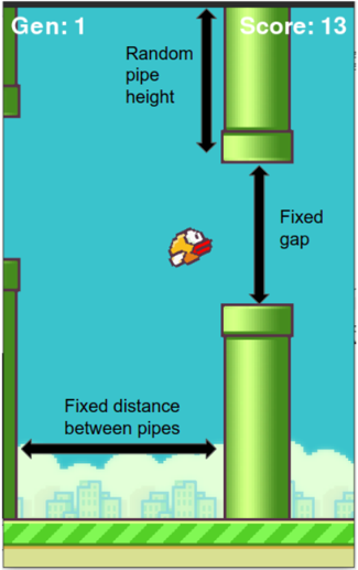t \quad ( 4 )$$ Eq. (1) determines the vertical displacement of the agent, where a is the acceleration that is a constant [12]. As shown in Fig. 1. Details of the game environment [10] <details> <summary>Image 1 Details</summary>  ### Visual Description ## Flappy Bird Game Diagram ### Overview The image is a diagram illustrating the setup of the Flappy Bird game environment. It highlights key parameters such as pipe height, gap size, and distance between pipes. The diagram also shows the current generation and score. ### Components/Axes * **Title**: None explicitly stated, but the image represents the Flappy Bird game environment. * **Labels**: * "Gen: 1" (Generation 1) - Located at the top-left. * "Score: 13" - Located at the top-right. * "Random pipe height" - Label with a double-headed arrow pointing to the top pipe. * "Fixed gap" - Label with a double-headed arrow pointing to the space between the top and bottom pipes. * "Fixed distance between pipes" - Label with a double-headed arrow pointing to the horizontal distance between two sets of pipes. ### Detailed Analysis or ### Content Details * **Game Elements**: * **Bird**: A small, yellow and orange bird is positioned in the center of the screen. * **Pipes**: Green pipes are placed vertically, with a gap between them for the bird to fly through. The height of the pipes varies randomly. * **Background**: The background is a light blue color, with a ground area at the bottom consisting of green grass and a cityscape. * **Parameters**: * The height of the pipes is described as "Random pipe height". * The gap between the pipes is described as "Fixed gap". * The distance between the sets of pipes is described as "Fixed distance between pipes". * **Game State**: * The game is currently in "Gen: 1" (Generation 1). * The current "Score: 13". ### Key Observations * The diagram emphasizes the key parameters that define the game's difficulty and challenge. * The "Random pipe height" suggests that the game dynamically adjusts the pipe configuration. * The "Fixed gap" and "Fixed distance between pipes" provide constraints within which the bird must navigate. ### Interpretation The diagram provides a visual representation of the Flappy Bird game environment and highlights the key parameters that influence gameplay. The combination of random pipe heights and fixed gaps and distances creates a challenging and unpredictable experience for the player. The "Gen" and "Score" indicate the game's progress and performance metrics. The diagram is useful for understanding the game's mechanics and the challenges it presents. 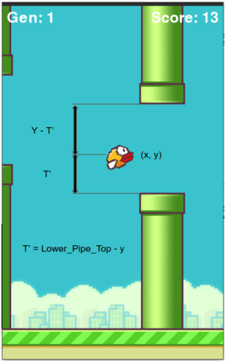</details> the Fig. 2, the y coordinate of the agent, the distance between the top pipe and the agent (y - T') and the distance between the bottom pipe and the agent (T') are the inputs to the neural network. The gap between the top and the bottom pipe is fixed to 320 pixels, and the heights are randomly generated. The distance between subsequent pipes is also kept constant. With respect to the NEAT algorithm, the fitness of the agent is determined by the number of pipes that the agent is able to cross without collision. As soon as the agent collides with the pipe, hits the roof, or falls down to the ground, the agent is removed from the environment. The performance of the algorithm depends on the initial population that is taken into consideration. The activation function used is the hyperbolic tangent function. The mutation rate is kept at 0.03. The encoding of the chromosome is shown in Table. I. The weight of the connection from a node in a layer to another node in the other layer and the dropped value is also considered as part of the encoding. If the connection is to be dropped, it Fig. 2. Parameters required as input to the NN <details> <summary>Image 2 Details</summary>  ### Visual Description ## Game Diagram: Flappy Bird State ### Overview The image depicts a state within a Flappy Bird game environment. It shows the bird's position relative to the pipes, along with game information such as the generation number and score. The diagram also includes annotations indicating how certain distances are calculated. ### Components/Axes * **Game Environment:** The background shows a blue sky with pixelated clouds and a cityscape at the bottom. A green ground with stripes is also visible. * **Pipes:** Two green pipes are present, one extending downwards from the top of the screen and the other extending upwards from the bottom. * **Bird:** A yellow and orange bird is positioned in the center of the screen, labeled with coordinates (x, y). * **Labels:** * "Gen: 1" (top-left) indicates the generation number. * "Score: 13" (top-right) indicates the current score. * "Y - T'" (left side, above the bird) represents the distance between the top pipe and a point relative to the bird's vertical position. * "T'" (left side, below the bird) represents a distance. * "T' = Lower\_Pipe\_Top - y" (bottom-left) defines T' as the difference between the top of the lower pipe and the bird's y-coordinate. * **Arrows:** Two vertical arrows indicate the distance "Y - T'" and "T'". A horizontal arrow points from the bird to the label "(x, y)". ### Detailed Analysis or ### Content Details * The bird is positioned approximately in the horizontal center of the screen. * The vertical distance between the top and bottom pipes appears to be relatively small. * The equation "T' = Lower\_Pipe\_Top - y" suggests that T' represents the vertical distance between the top of the lower pipe and the bird's vertical position. * "Y - T'" likely represents the distance between the top of the upper pipe and the bird's vertical position, adjusted by T'. ### Key Observations * The game is in its first generation, and the player has a score of 13. * The diagram focuses on the spatial relationship between the bird and the pipes, particularly the vertical distances. * The annotations provide insight into how the game might calculate distances for collision detection or AI purposes. ### Interpretation The image provides a snapshot of the Flappy Bird game state, highlighting the key parameters used in determining the bird's position relative to the obstacles. The equation for T' is crucial, as it likely plays a role in the game's logic for determining success or failure. The variables "Y - T'" and "T'" are used to calculate the distance between the bird and the pipes. The game uses these distances to determine if the bird has collided with a pipe. The diagram suggests that the game uses the bird's y-coordinate and the position of the lower pipe to calculate T'. This value is then used to calculate the distance between the bird and the pipes. 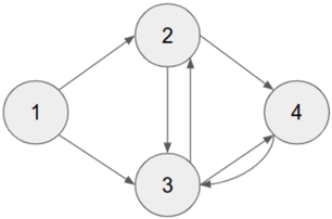</details> is encoded with the value 0 otherwise, it has the value 1. With reference to Fig. 3 and Table. I, the edges between Fig. 3. Diagramatic view of the encoded chromosome in Table I <details> <summary>Image 3 Details</summary>  ### Visual Description ## Diagram: Directed Graph ### Overview The image shows a directed graph with four nodes labeled 1, 2, 3, and 4. The arrows indicate the direction of the relationships between the nodes. ### Components/Axes * **Nodes:** Four nodes represented as circles, labeled 1, 2, 3, and 4. * **Edges:** Directed edges (arrows) connecting the nodes. ### Detailed Analysis * Node 1 has outgoing edges to Node 2 and Node 3. * Node 2 has outgoing edges to Node 3 and Node 4. * Node 3 has outgoing edges to Node 2. * Node 4 has outgoing edges to Node 3 and a self-loop (an edge back to itself). ### Key Observations * The graph is directed, meaning the relationships between nodes are not necessarily reciprocal. * Node 4 has a self-loop, indicating a relationship with itself. * There is a cycle between nodes 2 and 3. * Node 1 is the only node with no incoming edges. ### Interpretation The diagram represents a system with four components (nodes) and the relationships (edges) between them. The direction of the arrows indicates the flow or influence between the components. The self-loop on Node 4 suggests a feedback mechanism or self-reinforcing behavior within that component. The cycle between nodes 2 and 3 indicates a reciprocal relationship or feedback loop between these two components. Node 1 appears to be an initial or source node, as it has no incoming edges. 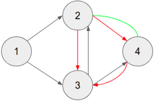</details> TABLE I ENCODING OF A CHROMOSOME BEFORE CROSSOVER AND MUTATION | Weight | 0.25 | 2.31 | 1.55 | 0.98 | 5.11 | 1.17 | 0.07 | |----------|--------|--------|--------|--------|--------|--------|--------| | From | 1 | 2 | 3 | 1 | 3 | 4 | 2 | | To | 2 | 3 | 2 | 3 | 4 | 3 | 4 | | Enabled | 1 | 0 | 1 | 1 | 1 | 1 | 1 | the nodes are represented by the rows 'From' and 'To'. The Table. I shows the encoding of the network before mutation. After the mutation, or rather after topology augmentation, the encoding of the edges is shown in Table. II. The resultant connections are shown in Fig. 4. The edges that are in red are the edges that were dropped, and the edges that are in green are the ones that have been added as a result of the mutation. The cross-over process happens between any two randomly selected parents. The next population is determined by the fitness of the individual agents. Fig. 4. Diagramatic view of the encoded chromosome in Table. II <details> <summary>Image 4 Details</summary>  ### Visual Description ## Diagram: Directed Graph with Colored Edges ### Overview The image depicts a directed graph consisting of four nodes labeled 1, 2, 3, and 4. The nodes are connected by edges, some of which are colored differently (gray, red, and green) to indicate different relationships or properties. ### Components/Axes * **Nodes:** Four nodes labeled 1, 2, 3, and 4, arranged in a roughly diamond shape. * **Edges:** Directed edges (arrows) connecting the nodes. The edges are colored gray, red, or green. ### Detailed Analysis * **Node 1:** * Has a gray edge directed towards Node 2. * Has a gray edge directed towards Node 3. * **Node 2:** * Has a gray edge directed towards Node 4. * Has a red edge directed towards Node 3. * Has a green edge directed towards Node 4. * **Node 3:** * Has a gray edge directed towards Node 2. * Has a red edge directed towards Node 4. * **Node 4:** * Has a gray edge directed towards Node 3. * Has a red edge directed towards Node 4 (self-loop). ### Key Observations * The graph is directed, meaning the edges have a specific direction. * The colors of the edges (gray, red, green) likely represent different types of relationships or properties between the nodes. * Node 4 has a self-loop (an edge that starts and ends at the same node). ### Interpretation The diagram represents a network or system with four components (nodes) and relationships (edges) between them. The colors of the edges could represent different types of interactions, strengths of connections, or other properties. The self-loop on Node 4 indicates a feedback mechanism or a recurring process within that component. Without further context, the specific meaning of the colors and the overall purpose of the graph cannot be determined. </details> TABLE II ENCODING OF A CHROMOSOME AFTER CROSSOVER AND MUTATION | Weight | 0.25 | 5.11 | 1.17 | 0.98 | 2.31 | 1.55 | 0.07 | |----------|--------|--------|--------|--------|--------|--------|--------| | From | 1 | 2 | 4 | 1 | 3 | 3 | 4 | | To | 3 | 4 | 2 | 4 | 2 | 4 | 3 | | Enabled | 1 | 1 | 1 | 0 | 1 | 1 | 0 | ## IV. 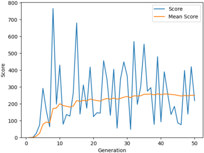RESULTS The implementation of the algorithm requires no historic data or any dataset. The algorithm makes use of the sensory data perceived from the environment by the artificial agent as the program runs. The inputs to the algorithm are the y position of the agent, the vertical distance of the agent from the top pipe, and the vertical distance of the agent from the lower pipe. The output of the algorithm is the action that the agent is to take i.e. jump or drop down owing to gravity. NEAT algorithm was implemented by taking different initial populations. Fig. 5, Fig. 6 and Fig. 7 shows the average score and the scores reached in every generation, when the game is played by the agents over 50 generations. The change in the average scores Fig. 5. Gameplay when initial population is 80 <details> <summary>Image 5 Details</summary>  ### Visual Description ## Line Chart: Score vs. Generation ### Overview The image is a line chart showing the "Score" and "Mean Score" over 50 "Generations". The "Score" line fluctuates significantly, while the "Mean Score" line shows a smoother, generally increasing trend. ### Components/Axes * **X-axis:** "Generation", ranging from 0 to 50 in increments of 10. * **Y-axis:** "Score", ranging from 0 to 800 in increments of 100. * **Legend:** Located in the top-right corner. * Blue line: "Score" * Orange line: "Mean Score" ### Detailed Analysis * **Score (Blue Line):** * Trend: Highly volatile, with large spikes and dips. * Initial values: Starts at approximately 0 at Generation 0. * Notable peaks: Around Generation 8 (approximately 770), Generation 16 (approximately 680), Generation 32 (approximately 580). * Notable dips: Around Generation 12 (approximately 120), Generation 38 (approximately 80). * Final value: Approximately 220 at Generation 50. * **Mean Score (Orange Line):** * Trend: Generally increasing, with smoother fluctuations compared to the "Score" line. * Initial values: Starts at approximately 0 at Generation 0. * Increases to approximately 190 by Generation 10. * Plateaus around 220-260 between Generations 20 and 50. * Final value: Approximately 250 at Generation 50. ### Key Observations * The "Score" exhibits high variance, indicating significant fluctuations in performance across generations. * The "Mean Score" provides a more stable representation of the overall performance trend, showing a gradual improvement over generations. * The "Score" line has several peaks and valleys, suggesting periods of both high and low performance. * The "Mean Score" plateaus after Generation 30, indicating that the average performance stabilizes. ### Interpretation The chart likely represents the performance of an algorithm or system over multiple generations. The "Score" reflects the instantaneous performance in each generation, while the "Mean Score" represents the average performance up to that generation. The high volatility of the "Score" suggests that individual generations can have widely varying outcomes, possibly due to randomness or sensitivity to initial conditions. The increasing "Mean Score" indicates that, on average, the system is improving over time, even though individual generations may perform poorly. The plateau in "Mean Score" after Generation 30 suggests that the system has reached a point of diminishing returns, where further generations do not lead to significant improvements in average performance. 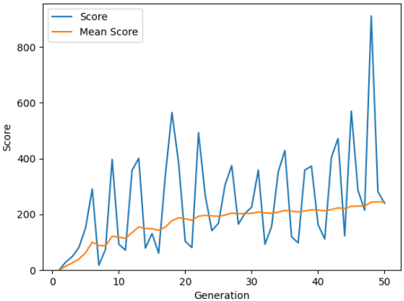</details> over the change in the initial population is separately shown in Fig. 6. Gameplay when initial population is 100 <details> <summary>Image 6 Details</summary>  ### Visual Description ## Line Chart: Score vs. Generation ### Overview The image is a line chart displaying the "Score" and "Mean Score" over 50 generations. The x-axis represents the generation number, and the y-axis represents the score. The chart shows the fluctuation of the score and the trend of the mean score over the generations. ### Components/Axes * **Title:** There is no explicit title on the chart. * **X-axis:** * Label: "Generation" * Scale: 0 to 50, with tick marks every 10 units (0, 10, 20, 30, 40, 50). * **Y-axis:** * Label: "Score" * Scale: 0 to 800, with tick marks every 200 units (0, 200, 400, 600, 800). * **Legend:** Located in the top-left corner. * "Score" - represented by a blue line. * "Mean Score" - represented by an orange line. ### Detailed Analysis * **Score (Blue Line):** * Trend: Highly volatile, with peaks and troughs throughout the generations. Generally increasing over time, with a large spike at generation 50. * Data Points: * Generation 0: Score is approximately 0. * Generation 5: Score is approximately 100. * Generation 10: Score fluctuates between approximately 50 and 400. * Generation 20: Score fluctuates between approximately 75 and 600. * Generation 30: Score fluctuates between approximately 100 and 400. * Generation 40: Score fluctuates between approximately 100 and 500. * Generation 50: Score reaches a peak of approximately 875. * **Mean Score (Orange Line):** * Trend: Generally increasing over time, with less volatility than the "Score" line. * Data Points: * Generation 0: Mean Score is approximately 0. * Generation 5: Mean Score is approximately 50. * Generation 10: Mean Score is approximately 150. * Generation 20: Mean Score is approximately 175. * Generation 30: Mean Score is approximately 200. * Generation 40: Mean Score is approximately 225. * Generation 50: Mean Score is approximately 250. ### Key Observations * The "Score" fluctuates significantly, indicating variability in performance across generations. * The "Mean Score" shows a gradual increase, suggesting an overall improvement in performance as the generations progress. * The large spike in "Score" at generation 50 is a notable outlier. ### Interpretation The chart likely represents the performance of a genetic algorithm or similar optimization process. The "Score" represents the performance of the best individual in each generation, while the "Mean Score" represents the average performance of the population. The increasing "Mean Score" suggests that the algorithm is successfully evolving better solutions over time. The volatility of the "Score" indicates that there is still significant variation in the population, and the spike at generation 50 suggests that a particularly good solution was found in that generation. The difference between the score and the mean score indicates the diversity of the population. 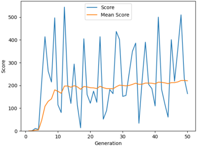</details> Fig. 7. Gameplay when initial population is 120 <details> <summary>Image 7 Details</summary>  ### Visual Description ## Line Chart: Score vs. Generation ### Overview The image is a line chart displaying the "Score" and "Mean Score" over 50 generations. The "Score" line fluctuates significantly, while the "Mean Score" line shows a gradual increase and then stabilizes. ### Components/Axes * **X-axis:** Generation, labeled from 0 to 50 in increments of 10. * **Y-axis:** Score, labeled from 0 to 500 in increments of 100. * **Legend (top-center):** * Blue line: "Score" * Orange line: "Mean Score" ### Detailed Analysis * **Score (Blue Line):** * Trend: Highly volatile, with large fluctuations between generations. * Initial Values: Starts near 0 at generation 0. * Peak Values: Reaches peaks around 400-500 at various generations (e.g., around generations 10, 25, 40, and 50). * Low Values: Drops to near 0 at several points (e.g., around generations 15, 20, 30, and 45). * **Mean Score (Orange Line):** * Trend: Initially increases rapidly, then stabilizes around a value between 180 and 220. * Initial Values: Starts near 0 at generation 0. * Stabilized Value: Reaches a plateau around 200 after approximately 10 generations. * Final Value: Ends around 220 at generation 50. ### Key Observations * The "Score" exhibits high variance, indicating significant performance differences between individual generations. * The "Mean Score" provides a smoother representation of the overall performance trend, showing an initial learning phase followed by stabilization. * The "Score" line frequently dips to very low values, suggesting occasional poor-performing generations despite the overall increasing trend in the "Mean Score." ### Interpretation The chart likely represents the performance of an algorithm or model over multiple generations. The volatile "Score" indicates that individual iterations can vary widely in their effectiveness. However, the "Mean Score" suggests that, on average, the algorithm improves over time, eventually reaching a stable level of performance. The large fluctuations in the "Score" could be due to factors such as randomness in the algorithm, sensitivity to initial conditions, or exploration of different solution spaces. The stabilization of the "Mean Score" implies that the algorithm has converged to a relatively consistent level of performance. 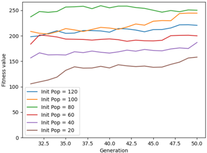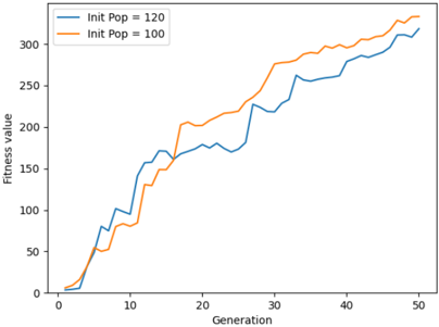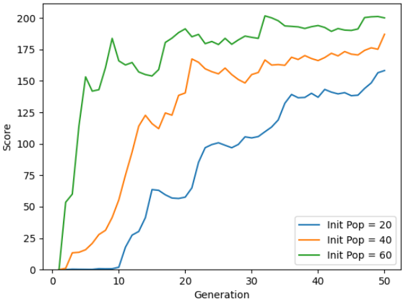</details> Fig. 8 for generations 30 to 50. The average score of the agent is steadily increasing from when the initial population is 20 to 100. The maximum score is observed when the population is 160. The average fitness value of the population is higher when the initial population size is 100. This is shown in Fig. 9. The initial training phase is less than 5 generations. When the initial population has fewer agents, it takes more generations to spike the average score of the game. This can be observed from Fig. 10. Table. III shows the average score and the maximum score gained by the agent over 50 generations. A maximum score of 1025 is obtained when the initial population is 160 and the gameplay run till 50 generations. ## CONCLUSION AND FUTURE SCOPE By using a 2D game, the performance of the algorithms can be determined very efficiently. Unlike simulation, the creation of an environment gives better control over the environment. Through various iterations by changing the initial population size, the average score gained by the agent has increased. The initial population of agents also affects the training speed. The more the agents, the quicker the training is done. The highest <details> <summary>Image 8 Details</summary>  ### Visual Description ## Line Chart: Fitness Value vs. Generation for Different Initial Population Sizes ### Overview The image is a line chart showing the relationship between "Fitness value" and "Generation" for different initial population sizes ("Init Pop"). The chart displays six lines, each representing a different initial population size, ranging from 20 to 120. The x-axis represents the generation number, and the y-axis represents the fitness value. ### Components/Axes * **X-axis:** Generation, with markers at 32.5, 35.0, 37.5, 40.0, 42.5, 45.0, 47.5, and 50.0. * **Y-axis:** Fitness value, ranging from 0 to 250, with implicit markers every 50 units. * **Legend:** Located in the bottom-left corner, it identifies each line by its corresponding initial population size: * Blue: Init Pop = 120 * Orange: Init Pop = 100 * Green: Init Pop = 80 * Red: Init Pop = 60 * Purple: Init Pop = 40 * Brown: Init Pop = 20 ### Detailed Analysis * **Blue Line (Init Pop = 120):** Starts at approximately 200, remains relatively stable between 200 and 210 until generation 45, then shows a slight upward trend to approximately 220 by generation 50. * **Orange Line (Init Pop = 100):** Starts at approximately 210, remains relatively stable between 210 and 220 until generation 45, then shows a slight upward trend to approximately 225 by generation 50. * **Green Line (Init Pop = 80):** Starts at approximately 240, remains relatively stable between 240 and 260 throughout the generations. * **Red Line (Init Pop = 60):** Starts at approximately 185, remains relatively stable between 190 and 200 until generation 45, then shows a slight upward trend to approximately 210 by generation 50. * **Purple Line (Init Pop = 40):** Starts at approximately 160, remains relatively stable between 160 and 170 until generation 45, then shows a slight upward trend to approximately 180 by generation 50. * **Brown Line (Init Pop = 20):** Starts at approximately 110, increases to approximately 140 by generation 40, remains relatively stable until generation 47.5, then shows a slight upward trend to approximately 160 by generation 50. ### Key Observations * Larger initial population sizes (80, 100, 120) generally result in higher fitness values. * The fitness values for all population sizes tend to stabilize after generation 40. * The fitness values for smaller population sizes (20, 40, 60) show a more pronounced increase over the generations compared to larger population sizes. ### Interpretation The chart suggests that a larger initial population size generally leads to a higher fitness value in this evolutionary process. However, the smaller initial population sizes show a more significant improvement in fitness over the generations, indicating that they may have more potential for further optimization. The stabilization of fitness values after generation 40 suggests that the evolutionary process may be reaching a plateau, and further generations may not result in significant improvements. The data demonstrates the impact of initial population size on the performance of an evolutionary algorithm, highlighting the trade-off between initial fitness and potential for improvement. </details> Generation Fig. 8. Average scores over initial population change (Gen 30 - Gen 50) <details> <summary>Image 9 Details</summary>  ### Visual Description ## Line Chart: Fitness Value vs. Generation for Different Initial Populations ### Overview The image is a line chart comparing the fitness value over generations for two different initial population sizes: 120 and 100. The x-axis represents the generation number, and the y-axis represents the fitness value. The chart shows how the fitness value changes over 50 generations for each initial population. ### Components/Axes * **X-axis:** Generation (0 to 50, increments of 10) * **Y-axis:** Fitness value (0 to 300, increments of 50) * **Legend (top-left):** * Blue line: Init Pop = 120 * Orange line: Init Pop = 100 ### Detailed Analysis * **Blue Line (Init Pop = 120):** * Trend: Generally increasing fitness value over generations. * Data Points: * Generation 0: ~0 * Generation 5: ~50 * Generation 10: ~100 * Generation 15: ~150 * Generation 20: ~170 * Generation 25: ~180 * Generation 30: ~230 * Generation 35: ~250 * Generation 40: ~280 * Generation 45: ~290 * Generation 50: ~320 * **Orange Line (Init Pop = 100):** * Trend: Generally increasing fitness value over generations. * Data Points: * Generation 0: ~0 * Generation 5: ~50 * Generation 10: ~80 * Generation 15: ~140 * Generation 20: ~200 * Generation 25: ~220 * Generation 30: ~230 * Generation 35: ~280 * Generation 40: ~290 * Generation 45: ~300 * Generation 50: ~310 ### Key Observations * Both lines show an overall upward trend, indicating that the fitness value increases with each generation. * The blue line (Init Pop = 120) initially increases more rapidly than the orange line (Init Pop = 100). * Around generation 20, the orange line catches up to the blue line. * From generation 35 onwards, the orange line (Init Pop = 100) appears to have a slightly higher fitness value than the blue line (Init Pop = 120). ### Interpretation The chart suggests that the initial population size affects the fitness value over generations. A larger initial population (120) may lead to a faster initial increase in fitness, but a smaller initial population (100) can eventually catch up and potentially surpass the fitness value of the larger population. This could be due to factors such as genetic diversity or the ability to explore different solutions more effectively with a smaller population. The data indicates that while a larger initial population might provide an early advantage, it doesn't necessarily guarantee a higher fitness value in the long run. </details> Fig. 9. Average Fitness of the population over initial population change <details> <summary>Image 10 Details</summary>  ### Visual Description ## Line Chart: Score vs. Generation for Different Initial Populations ### Overview The image is a line chart comparing the "Score" achieved over "Generation" for three different initial population sizes: 20, 40, and 60. The chart shows how the score evolves over 50 generations for each population size. ### Components/Axes * **X-axis:** Generation, ranging from 0 to 50. * **Y-axis:** Score, ranging from 0 to 200. * **Legend (bottom-right):** * Blue line: Init Pop = 20 * Orange line: Init Pop = 40 * Green line: Init Pop = 60 ### Detailed Analysis * **Init Pop = 20 (Blue Line):** * The score remains near 0 for the first 8 generations. * From generation 8 to 20, the score increases from approximately 0 to 60. * From generation 20 to 30, the score fluctuates between 55 and 65. * From generation 30 to 50, the score increases from approximately 65 to 160. * **Init Pop = 40 (Orange Line):** * The score remains near 0 for the first 3 generations. * From generation 3 to 15, the score increases from approximately 0 to 120. * From generation 15 to 35, the score increases from approximately 120 to 170. * From generation 35 to 50, the score fluctuates between 160 and 170. * **Init Pop = 60 (Green Line):** * The score increases rapidly from 0 to 150 within the first 7 generations. * From generation 7 to 20, the score fluctuates between 150 and 190. * From generation 20 to 35, the score remains relatively stable around 190. * From generation 35 to 50, the score fluctuates between 180 and 200. ### Key Observations * The green line (Init Pop = 60) consistently achieves the highest score throughout the generations. * The blue line (Init Pop = 20) shows the slowest initial growth but eventually reaches a score comparable to the orange line (Init Pop = 40) by generation 50. * All three lines show an initial period of rapid score increase, followed by a period of stabilization or slower growth. ### Interpretation The chart suggests that a larger initial population size (Init Pop = 60) leads to a faster and higher score in the early generations. However, the smaller initial population sizes eventually catch up, indicating that the initial population size has a greater impact on the initial learning rate than the final performance. The fluctuations in the score suggest that there is some variability in the performance of each generation, possibly due to random factors in the simulation or learning process. The data demonstrates that increasing the initial population size can improve the initial performance of the system, but it may not necessarily lead to a significantly higher final score. </details> Fig. 10. Speed of agents getting trained over initial population change | Initial Population | Average Score | Max Score | |----------------------|-----------------|-------------| | 20 | 158.2 | 583 | | 40 | 187.04 | 771 | | 60 | 200.06 | 756 | | 80 | 250.28 | 765 | | 100 | 244.56 | 911 | | 120 | 220.66 | 544 | | 140 | 255.82 | 565 | | 160 | 293.72 | 1025 | average score is obtained when the initial population is set to 100 individuals. It can be concluded that the performance of the algorithm increases as the initial population is increased. The implemented algorithm can be extended to making use of Reinforcement Learning with multiple agents and using Augmented Topologies along with the Deep Q-Learning model. ## REFERENCES - [1] M. G. Cordeiro, Paulo B. S. Serafim, Yuri B. Nogueira, 'A Minimal Training Strategy to Play Flappy Bird Indefinitely with NEAT', 2019 18th Brazilian Symposium on Computer Games and Digital Entertainment (SBGames), pp. 384-390, DOI: 10.1109/SBGames.2019.00014. - [2] Evgenia Papavasileiou, Jan Cornelis and Bart Jansen, 'A Systematic Literature Review of the Successors of 'NeuroEvolution of Augmenting Topolo- gies', Evolutionary Computation, vol: 29, Issue: 1, March 2021, pp. 1-73, DOI: 10.1162/evcoa00282. - [3] Inseok Oh, Seungeun Rho, Sangbin Moon and Seongho Son, 'Creating Pro-Level AI for a Real-Time Fighting Game Using Deep Reinforcement Learning', IEEE Transactions on Games, 2021, pp. 1-10, doi: 10.1109/TG.2021.3049539. - [4] Botong Liu, 'Implementing Game Strategies Based on Reinforcement Learning', ICRAI 2020: 2020 6th International Conference on Robotics and Artificial Intelligence, November 2020, pp 53-56, DOI: https://doi.org/10.1145/3449301.3449311. - [5] Evalds Urtans, Agris Nikitenko, 'Survey of Deep Q-Network variants in PyGame Learning Environment', ICDLT '18: Proceedings of the 2018 2nd International Conference on Deep Learning Technologies, June 2018, pp 27-36, DOI: https://doi.org/10.1145/3234804.3234816. - [6] Tai Vu, Leon Tran, 'FlapAI Bird: Training an Agent to Play Flappy Bird Using Reinforcement Learning Techniques', experimental projects with community collaborators, 2020, DOI: https://doi.org/10.48550/arXiv.2003.09579. - [7] Andre Brandao, Pedro Pires, Petia Georgieva, 'Reinforcement Learning and Neuroevolution in Flappy Bird Game', Pattern Recognition and Image Analysis, 2019, pp.225-236, DOI: DOI:10.1007/978-3-030-31332620. - [8] Yash Mishra, Vijay Kumawat, Selvakumar Kamalanathan, 'Performance Analysis of Flappy Bird Playing Agent Using Neural Network and Genetic Algorithm', Information, Communication and Computing Technology, 2019, pp.253-265, DOI:10.1007/978-981-15-1384-821. - [9] A. McIntyre, M. Kallada, C. G. Miguel, and C. F. da Silva, 'neatpython,' https://github.com/CodeReclaimers/neat-python. - [10] T. Ruscica and J. Keromnes, 'Flappy Bird game images', https://github.com/techwithtim/NEAT-Flappy-Bird/tree/master/imgs. - [11] S. Kumar, 'Understand Types of Environments in Artificial Intelligence', https://www.aitude.com/understand-types-of-environments-inartificial-intelligence/, 2020. - [12] D. Zhu, 'How I Built an Intelligent Agent to Play Flappy Bird', Analytics Vidhya, 2020.