2209.03152v1

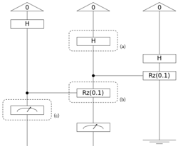
# ArXiv Paper 2209.03152v1 ## A multiclass Q-NLP sentiment analysis experiment using DisCoCat Victor Martinez IBM victor.martinez@ibm.com Guilhaume Leroy-Meline IBM guilhaume@fr.ibm.com | ψ 〉 = | ψ 1 〉 ⊗ ... ⊗| ψ n 〉 . The Born rule can be used to retrieve the probability of measuring the system | ψ 〉 in state x by computing p ( x ) = | 〈 x | ψ 〉 | 2 . Furthermore, one can perform elementary operations on those qubits through quantum gates. Those gates can be represented as linear algebra operations on | ψ 〉 and correspond to instructions that will be physically performed on the quantum computer. The gates used along with their parameters is referred to as an Ansatz . An example of such Ansatz is given in Figure 1. Figure 1: A three qubit quantum circuit U with different gates. (a) represents a Hadamard gate, (b) a parameterized controlled Z-Rotation and (c) a measurement operation <details> <summary>Image 1 Details</summary>  ### Visual Description ## Quantum Circuit Diagram: Three-State Quantum Processing Flow ### Overview The image depicts three quantum circuit diagrams (labeled a, b, c) illustrating sequential quantum gate operations on a single qubit (labeled "0"). Each diagram shows quantum gates (Hadamard "H" and Rotational "Rz(0.1)"), measurement operations, and connectivity between components. The circuits are vertically stacked with horizontal connections indicating qubit state transitions. ### Components/Axes - **Qubit**: Labeled "0" at the top of all diagrams, representing the quantum state being manipulated. - **Gates**: - **H (Hadamard)**: Appears in all three diagrams, applied to qubit 0. - **Rz(0.1)**: Rotational gate with phase shift 0.1, present in diagrams (a) and (b). - **Measurement**: Symbolized by a meter icon (□ with arrow), present in diagrams (b) and (c). - **Connectivity**: Dotted lines indicate optional or conditional paths (e.g., measurement in diagram b). - **Labels**: Diagrams are explicitly labeled (a), (b), (c) on the right side. ### Detailed Analysis 1. **Diagram (a)**: - **Structure**: Qubit 0 → H gate → Rz(0.1) gate. - **Flow**: Initial Hadamard operation creates superposition, followed by a phase rotation (Rz(0.1)). - **Notable**: No measurement; represents state preparation only. 2. **Diagram (b)**: - **Structure**: Qubit 0 → H gate → Rz(0.1) gate → Measurement. - **Flow**: Adds measurement after Rz(0.1), collapsing the quantum state. - **Notable**: Dotted line suggests conditional execution or alternative paths. 3. **Diagram (c)**: - **Structure**: Qubit 0 → H gate → Measurement. - **Flow**: Simplest configuration, measuring directly after Hadamard. - **Notable**: Lacks Rz(0.1), emphasizing baseline measurement behavior. ### Key Observations - **Gate Order Sensitivity**: Diagram (a) vs. (c) shows how Rz(0.1) modifies the qubit state before measurement. - **Measurement Impact**: Diagram (b) introduces state collapse, altering subsequent operations. - **Phase Rotation**: Rz(0.1) introduces a small phase shift (0.1 radians), critical for interference effects in quantum algorithms. ### Interpretation This diagram illustrates foundational quantum processing steps: 1. **State Preparation** (Diagram a): Combines superposition (H) and phase manipulation (Rz) to encode information. 2. **Measurement** (Diagrams b/c): Demonstrates how measurement timing affects outcomes. Diagram (b) shows intermediate measurement after phase rotation, while (c) measures the raw superposition. 3. **Conditional Execution**: The dotted line in (b) implies classical control logic, enabling dynamic circuit adaptation based on measurement results. The progression from (a) to (c) highlights trade-offs between gate complexity and measurement granularity. The Rz(0.1) gate’s minimal phase shift suggests applications in precision-sensitive algorithms (e.g., quantum sensing), while the absence of Rz in (c) represents a baseline for comparison. The measurement placement directly impacts the qubit’s final state, emphasizing the quantum-classical interface challenges. </details> This allows us to define a generic way of performing supervised machine learning tasks using variational quantum circuits. The data is first encoded in a quantum state | ψ 0 〉 . We then apply a parameterized quantum circuit U ( θ ) to | ψ 0 〉 , where θ is trained with the labeled dataset. We measure the wave function | ψ 〉 = U ( θ ) | ψ 0 〉 . The result being probabilistic by nature, we perform this operation multiple times to retrieve the outcome probabilities. Figure 2: Pipeline to perform supervised machine learning tasks on a quantum computer <details> <summary>Image 2 Details</summary>  ### Visual Description ## Flowchart: Quantum Circuit Processing Workflow ### Overview The diagram illustrates a quantum computing workflow involving data encoding, quantum circuit execution, measurement, and iterative parameter adjustment. The process is cyclical, with feedback from measurement results used to refine the quantum circuit's parameters. ### Components/Axes 1. **Blocks**: - **Encoding**: Input labeled "Data" → Output labeled |ψ₀⟩. - **Quantum circuit U(θ)**: Input |ψ₀⟩ → Output |ψ⟩ = U(θ)|ψ₀⟩. - **Measurement**: Output labeled "Result". 2. **Arrows**: - Data → Encoding → Quantum circuit → Measurement → Result. - Feedback loop: Measurement → Adjust θ → Quantum circuit. 3. **Text Labels**: - "Adjust θ using gradient free methods" (feedback loop). ### Detailed Analysis - **Encoding**: Converts raw data into a quantum state |ψ₀⟩. - **Quantum circuit U(θ)**: Applies parameterized unitary operations (θ) to |ψ₀⟩, producing |ψ⟩. - **Measurement**: Collapses |ψ⟩ to classical results. - **Parameter adjustment**: θ is iteratively optimized using gradient-free methods (e.g., genetic algorithms, simulated annealing). ### Key Observations - The workflow is **cyclical**, emphasizing iterative refinement of θ. - No explicit numerical values or trends are provided; the focus is on process flow. - The feedback loop highlights **adaptive optimization** without gradient-based methods. ### Interpretation This diagram represents a **variational quantum algorithm** (VQA) framework, where: 1. **Data encoding** initializes the quantum state. 2. **Parameterized circuits** (U(θ)) explore the quantum state space. 3. **Measurement outcomes** guide the optimization of θ via gradient-free techniques, avoiding reliance on classical gradients (common in noisy intermediate-scale quantum (NISQ) devices). 4. The absence of explicit numerical data suggests the diagram is conceptual, emphasizing methodology over empirical results. The process underscores the interplay between quantum computation and classical optimization, critical for near-term quantum applications like quantum machine learning or error mitigation. </details> ## Abstract Sentiment analysis is a branch of Natural Language Processing (NLP) which goal is to assign sentiments or emotions to particular sentences or words. Performing this task is particularly useful for companies wishing to take into account customer feedback through chatbots or verbatim. This has been done extensively in the literature using various approaches, ranging from simple models to deep BERT neural networks. In this paper, we will tackle sentiment analysis in the Noisy Intermediate Scale Computing (NISQ) era, using the DisCoCat model of language. We will first present the basics of quantum computing and the DisCoCat model. This will enable us to define a general framework to perform NLP tasks on a quantum computer. We will then extend the twoclass classification that was performed by Lorenz et al. (2021) to a four-class sentiment analysis experiment on a much larger dataset, showing the scalability of such a framework. ## 1 Introduction to Quantum Computing For a more complete introduction to Quantum Computing, the reader is invited to read Nielsen and Chuang (2010). The base unit of any quantum computer is the qubit , which can be seen as a two-dimensional complex vector represented by its wave function | ψ 〉 = α | 0 〉 + β | 1 〉 . α and β are complex numbers, which squared amplitude is the probability of measuring the wave function in the associated quantum state. In the same way, we may consider the system made of two uncorrelated qubits | ψ 1 〉 = α 1 | 0 〉 + β 1 | 1 〉 and | ψ 2 〉 = α 2 | 0 〉 + β 2 | 1 〉 . The joint system can be written | ψ 〉 = α 1 α 2 | 00 〉 + α 1 β 2 | 01 〉 + β 1 α 2 | 10 〉 + β 1 β 2 | 11 〉 , or equivalently | ψ 〉 = | ψ 1 〉 ⊗ | ψ 2 〉 , where ⊗ represents the tensor product. Using this notation, we can generalize to n uncorrelated qubits, which joint system's is written The choice of Ansatz for U is crucial, since the design of the circuit has to be chosen so that the result is a function of the outcome probabilities. In some cases, the result is not directly a function of the outcome probabilities of the n qubits, but a function of the outcome probabilities of n -r qubits under some conditions that have to satisfy the other r qubits. In Figure 1, we could expect the second and third qubits to be 0 for our run to be valid, the result only being given by the first qubit. This requires some additional post-selection, forcing us to only keep the runs where the conditions on the r qubits are met. This will be particularly important in the following, since we will expect 0 effects on many of our qubits. 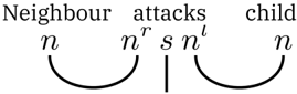## 2 The DisCoCat model The categorical compositional distributional (DisCoCat) model of meaning is based on the framework of compact closed category, and the reader is invited to read Coecke et al. (2010) for a complete introduction. The main idea behind DisCoCat is to decompose the language into two components. We first associate each word a meaning, as commonly done using word embedding. This word embedding can be done by projecting the words on a vector space made of basis vocabulary (for example 700 words). The second component of our language is the syntactic structure of the sentences, which is commonly represented by a syntax tree. How the words relate to each other tells us the global meaning of the sentence. An example of such syntax tree can be found in Figure 3 Figure 3: Syntax tree of a simple noun-verb-noun sentence <details> <summary>Image 3 Details</summary>  ### Visual Description ## Diagram: Causal Relationship Between Neighbour, Attacks, and Child ### Overview The diagram illustrates a directional relationship between three entities: "Neighbour," "attacks," and "child." Arrows indicate the flow of interaction, with labels specifying the nature of the relationships. Mathematical notation is embedded in the labels to denote variables and operations. ### Components/Axes - **Nodes**: - **Neighbour**: Labeled `n` (lowercase italic `n`). - **Attacks**: Labeled `n^r s n^t` (superscript `r` on `n`, followed by `s`, then superscript `t` on `n`). - **Child**: Labeled `n` (same as Neighbour). - **Arrows**: - **Neighbour → Attacks**: Labeled "attacks." - **Attacks → Child**: Labeled "child." ### Detailed Analysis - **Node Labels**: - The "Neighbour" and "Child" nodes share the same variable `n`, suggesting they may represent the same entity in different contexts or roles. - The "Attacks" node uses a compound formula `n^r s n^t`, which could imply an operation (e.g., multiplication, concatenation) between modified instances of `n` (e.g., `n^r` and `n^t`). - **Arrow Labels**: - The arrow from "Neighbour" to "Attacks" is explicitly labeled "attacks," indicating the action or event. - The arrow from "Attacks" to "Child" is labeled "child," suggesting the target or outcome of the attack. ### Key Observations - The diagram implies a causal chain: the Neighbour (`n`) initiates an "attacks" action, which is mathematically represented as `n^r s n^t`, and this action directly affects the Child (`n`). - The reuse of `n` for both Neighbour and Child may indicate a shared variable or a recursive relationship (e.g., the Child is a subordinate or dependent of the Neighbour). ### Interpretation This diagram likely models a system where an entity (Neighbour) exerts influence or harm (attacks) on another entity (Child), with the "attacks" node acting as an intermediary. The formula `n^r s n^t` could represent a transformation or interaction between the Neighbour and Child, such as: - **Mathematical**: A function where `n^r` and `n^t` are variables modified by exponents `r` and `t`, combined via an operation `s`. - **Logical**: A rule where the Neighbour's action (`n^r`) combined with a secondary factor (`n^t`) results in an attack on the Child. The bidirectional use of `n` for Neighbour and Child might suggest symmetry or reciprocity in the relationship, though the directional arrows clarify the primary flow from Neighbour to Child via the "attacks" node. This structure could apply to fields like game theory, social dynamics, or algorithmic modeling, where entities interact through defined operations. </details> Taking into account both those aspects can be done through the use of tensor products by following the below steps. 1. Compose the tensor product of every word through their word embedding. s = w 1 ⊗ w 2 ⊗ ... ⊗ w n 2. Construct a linear map F corresponding to the sentence's syntax tree. 3. Apply the linear map to the vector s , retrieving the meaning of the sentence S = F ( s ). 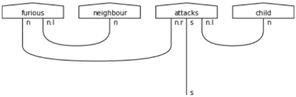Whythis DisCoCat model is particularly suited to quantum computing now becomes apparent. The Tensor Product Representation (TPR) requires to store the tensor product between n words, which scales exponentially in n . This makes this model unusable on classical computers, with several terabytes required to store a single sentence. However, as seen in Section 1, storing the tensor product of n words will scale linearly in the number of qubits . A more convenient way of handling these TPR is through the direct use of DisCoCat diagrams. This representation is illustrated in Figure 4, where boxes denote tensors and links tensor contractions. Figure 4: DisCoCat diagram of the sentence Furious neighbour attacks child <details> <summary>Image 4 Details</summary>  ### Visual Description ## Flowchart Diagram: State Transition Relationships ### Overview The diagram illustrates a state transition system with four primary nodes ("furious," "neighbour," "attacks," "child") connected by directional arrows. Each node contains sub-labels indicating state modifiers, and the flow suggests conditional transitions between states. The structure resembles a finite state machine or decision tree with explicit branching logic. ### Components/Axes - **Nodes**: 1. **Furious** (top-left) - Sub-labels: `n` (primary state), `n.l` (left modifier) 2. **Neighbour** (top-center) - Sub-label: `n` (primary state) 3. **Attacks** (top-right) - Sub-labels: `n.r` (right modifier), `s` (secondary state), `n.l` (left modifier) 4. **Child** (bottom-right) - Sub-label: `n` (primary state) - **Arrows**: - Horizontal connections between nodes - Vertical arrow from "Attacks" labeled `s` pointing downward to a terminal `s` state ### Detailed Analysis 1. **Furious Node**: - Primary state: `n` (neutral/normal) - Left modifier: `n.l` (possibly "neutral-left" or "non-lethal") - Outgoing arrows to "Neighbour" and "Attacks" 2. **Neighbour Node**: - Primary state: `n` - Single incoming arrow from "Furious" - Outgoing arrow to "Attacks" 3. **Attacks Node**: - Primary state: `n.r` (right modifier, possibly "neutral-right" or "non-relative") - Secondary state: `s` (terminal state) - Left modifier: `n.l` - Incoming arrows from "Furious" and "Neighbour" - Outgoing arrow to "Child" 4. **Child Node**: - Primary state: `n` - Single incoming arrow from "Attacks" 5. **Terminal State**: - Labeled `s` (possibly "stop" or "success") - Reached via vertical arrow from "Attacks" ### Key Observations - **Branching Logic**: The "Furious" state splits into two paths: one leading to "Neighbour" and another directly to "Attacks." - **Convergence Point**: Both "Furious" and "Neighbour" feed into "Attacks," creating a decision node. - **State Modifiers**: The use of `n.l`/`n.r` suggests directional or contextual variations of the neutral state. - **Terminal State**: The `s` state acts as an endpoint, disconnected from further transitions. ### Interpretation This diagram likely represents a conflict resolution or behavioral state machine: 1. **Initial State**: "Furious" (`n`) can escalate either through social interaction ("Neighbour") or direct action ("Attacks"). 2. **Modifiers**: The `n.l`/`n.r` labels imply contextual adjustments to the base state (e.g., "non-lethal" or "non-relative" attacks). 3. **Terminal Outcome**: All paths eventually lead to the `s` state, suggesting resolution or termination of the conflict sequence. 4. **Child State**: The "Child" node (`n`) may represent a reset or neutral outcome after an attack, though its single connection makes its role ambiguous. The structure emphasizes conditional transitions and state dependencies, with modifiers (`n.l`, `n.r`) potentially representing contextual flags influencing state behavior. The terminal `s` state acts as a system-wide endpoint, regardless of the path taken. </details> Using this quantum-suited representation of language as our data encoding process, we can take a closer look on how to perform NLP tasks. 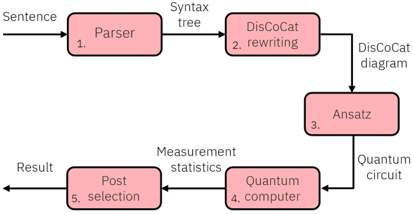## 3 General pipeline for QNLP tasks We can define a general framework for performing QNLP tasks with the steps below. 1. The sentence is parsed to obtain its syntax tree. For large datasets, this would require an automatic parser. 2. The syntax tree and the sentence are then combined to obtain the DisCoCat diagram which is written in an efficient way. 3. The DisCoCat diagram is mapped to a parameterized quantum circuit, which parameters are obtained through training. 4. The quantum circuit is compiled and executed on a quantum computer multiple times to retrieve the measurement statistics. 5. Post-processing is performed to select only runs where the r qubits have 0 effects. This gives us the final result. Those steps are summarised in Figure 5. In Section 4, those steps will be detailed on a real sentiment analysis task. Figure 5: Pipeline to perform NLP tasks on a quantum computer <details> <summary>Image 5 Details</summary>  ### Visual Description ## Flowchart: Quantum Processing Workflow ### Overview The image depicts a sequential workflow for processing a sentence through quantum computing stages. The process begins with a textual input ("Sentence") and progresses through five stages, culminating in a "Result". A feedback loop exists between "Ansatz" and "Quantum circuit". ### Components/Axes 1. **Nodes (Processes)**: - **1. Parser**: Converts "Sentence" into a syntax tree. - **2. DisCoCat rewriting**: Transforms the syntax tree into a DisCoCat diagram. - **3. Ansatz**: Represents a quantum circuit setup. - **4. Quantum computer**: Executes the quantum circuit. - **5. Post selection**: Finalizes the result. 2. **Arrows**: Indicate directional flow between stages. 3. **Branching**: "Ansatz" connects to both "Quantum circuit" and "Quantum computer". ### Detailed Analysis - **Input**: "Sentence" → **Parser** → Syntax tree. - **Rewriting**: Syntax tree → **DisCoCat rewriting** → DisCoCat diagram. - **Quantum Processing**: - DisCoCat diagram → **Ansatz** → Quantum circuit. - Quantum circuit → **Quantum computer** (feedback loop to Ansatz). - **Output**: Quantum computer → **Post selection** → Result. ### Key Observations - The workflow is linear with a single feedback loop between "Ansatz" and "Quantum circuit". - "Post selection" acts as the final decision-making stage before outputting the result. - "Ansatz" serves as a bridge between classical (DisCoCat) and quantum processing. ### Interpretation This flowchart illustrates a hybrid classical-quantum workflow: 1. **Classical Preprocessing**: The sentence is parsed and rewritten using DisCoCat (a probabilistic grammar framework) to structure the problem. 2. **Quantum Execution**: The structured problem ("Ansatz") is translated into a quantum circuit, which is iteratively optimized via feedback to the quantum computer. 3. **Result Finalization**: Post-selection (a quantum measurement technique) collapses the quantum state into a classical result. The feedback loop suggests iterative refinement of the quantum circuit design, likely to improve result accuracy or efficiency. The use of DisCoCat implies the problem involves probabilistic or context-sensitive rules, which are then mapped to quantum operations. </details> ## 4 Sentiment analysis experiment Lorenz et al. (2021) defined this framework and tested it on two-class meaning classification, yielding promising results. In this paper, we propose a similar approach to perform sentiment analysis on four emotions with a larger dataset. We restrict ourselves to the four most basic emotions: happiness, fear, anger, sadness . We will be using 3 and 4 words sentences, since we will be working with simulators or small size quantum computers. To circumvent the absence of automatic parser at our disposition, we create the sentences based on their syntax. We first start by defining the nouns, adjectives, transitive and intransitive verbs that will constitute our dataset. For each syntax - for example adjective-noun-verb-noun - we create every sentence possible matching this syntax. We therefore have access to the syntax of every sentence in our dataset. 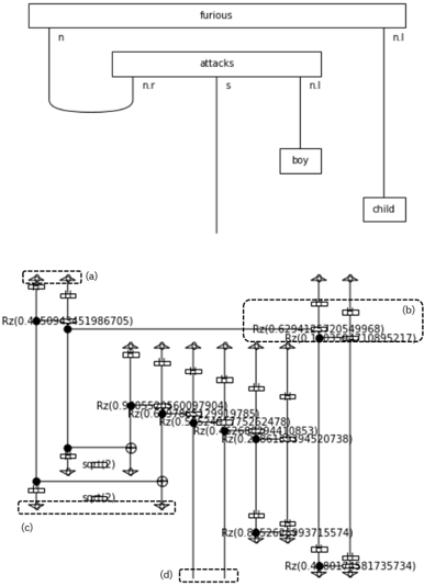| Nouns | Adjectives | Verbs | |-----------|--------------------------------------------|-----------------------------------------| | neighbour | anxious ecstatic irritated | attack scare anger amuse demoralise cry | | child | distressed blissful furious petrified | | | boy | frightened miserable young, blind cheerful | laugh dance scream | The second step, corresponding to the writing of the DisCoCat diagram, is done through Dis- coPy, an open source toolbox for computing with monoidal categories developed by Felice et al. (2021). This allows us to efficiently write the diagrams and map them to quantum circuits. An example of a DisCoCat diagram and its associated quantum circuit is depicted on Figure 6. The parametrisation of the Ansatz was done following Lorenz et al. (2021) and led to using two qubits for verbs and nouns. Figure 6: DisCoCat diagram and its associated quantum circuit. (a) Top qubits represent the initial qubits. (b) Gates applied to the qubits. (c) Bottom qubits expected to be 0. (d) Measured qubits giving the result probabilities <details> <summary>Image 6 Details</summary>  ### Visual Description ## Tree Diagram with Bar Chart: Hierarchical Classification and Metric Analysis ### Overview The image combines a hierarchical tree diagram at the top with a bar chart below. The tree diagram represents a classification structure, while the bar chart displays numerical metrics (Rz values) across four categories (a-d). Arrows indicate trends (upward/downward), and a legend distinguishes two data series ("squirt" and "squirt2"). ### Components/Axes #### Tree Diagram - **Root**: "furious" - **Branches**: - Left: "n" → splits into "n.r" and "s" - Right: "attacks" → splits into "boy" and "child" - **Labels**: All text is in English. #### Bar Chart - **X-axis**: Categories labeled (a), (b), (c), (d) - **Y-axis**: Rz values (e.g., Rz(0.45094451986705)) - **Legend**: - "squirt": Solid line with square markers - "squirt2": Dashed line with diamond markers - **Arrows**: Vertical arrows indicate trend direction (↑ for increase, ↓ for decrease). ### Detailed Analysis #### Tree Diagram - **Structure**: - "furious" (root) branches into "n" (left) and "attacks" (right). - "n" splits into "n.r" (left) and "s" (right). - "s" splits into "boy" (left) and "child" (right). - "attacks" splits into "boy" (left) and "child" (right). #### Bar Chart - **Category (a)**: - Two bars: - Solid (squirt): Rz(0.45094451986705) ↑ - Dashed (squirt2): Rz(0.6294125320549968) ↑ - **Category (b)**: - Three bars: - Solid: Rz(0.9550560097904) ↑ - Dashed: Rz(0.52465175262478) ↑ - Solid: Rz(0.60097904) ↑ - **Category (c)**: - Two bars: - Solid: Rz(0.85265993715574) ↑ - Dashed: Rz(0.480125581735734) ↑ - **Category (d)**: - Two bars: - Solid: Rz(0.5265993715574) ↑ - Dashed: Rz(0.480125581735734) ↑ ### Key Observations 1. **Tree Diagram**: - "boy" and "child" appear as terminal nodes under both "n.r" and "attacks," suggesting overlapping classifications. 2. **Bar Chart**: - **Trends**: - Category (a): Both series increase, with "squirt2" higher than "squirt." - Category (b): Mixed trends; "squirt" peaks at 0.955, while "squirt2" decreases. - Categories (c) and (d): "squirt" consistently higher than "squirt2," with gradual declines. - **Outliers**: - Category (b) "squirt" value (0.955) is the highest across all categories. - Category (b) "squirt2" value (0.5246) is the lowest among dashed lines. ### Interpretation - **Tree Diagram**: Represents a hierarchical taxonomy where "furious" is the root, and "boy" and "child" are nested under multiple parent nodes, indicating potential redundancy or shared attributes. - **Bar Chart**: - The Rz metric varies significantly across categories. - "squirt" (solid line) generally exhibits higher values than "squirt2" (dashed line), suggesting a performance or quality distinction between the two series. - The upward arrows in most bars imply positive trends, though category (b) shows a decline for "squirt2." - The overlapping "boy" and "child" nodes in the tree diagram may correlate with the Rz values in the bar chart, though no explicit link is provided. ### Critical Notes - The image lacks explicit axis titles or units for Rz, limiting interpretability. - The relationship between the tree diagram and bar chart is implied but not explicitly stated. - The legend’s placement (bottom-right) is standard, but the absence of a colorbar or additional context complicates cross-referencing. 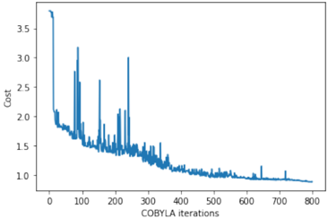</details> We run the circuits multiple time with postselection and measure the two qubits of interest to retrieve the outcome probabilities ( | 00 〉 , | 01 〉 , | 10 〉 , | 11 〉 ). These outcome probabilities directly give us the emotion linked to our sentence. The parameters of the Ansatz are trained using a Crossentropy loss and the outcome probabilities. The optimiser chosen was COBYLA, a gradient free optimizer. We split our dataset into a training and test dataset and plot the evolution of the cost function on the training dataset in Figure 7. Figure 7: Evolution of the cross entropy on the training dataset <details> <summary>Image 7 Details</summary>  ### Visual Description ## Line Graph: COBYLA Cost vs. Iterations ### Overview The image depicts a line graph illustrating the relationship between the number of COBYLA iterations and the associated cost. The graph shows a decreasing trend in cost over iterations, with notable fluctuations in the early stages. The y-axis represents "Cost" (ranging from 1.0 to 3.5), and the x-axis represents "COBYLA iterations" (ranging from 0 to 800). A single blue line, labeled "COBYLA" in the legend, tracks the cost metric across iterations. ### Components/Axes - **X-axis (Horizontal)**: Labeled "COBYLA iterations," with a linear scale from 0 to 800 in increments of 100. - **Y-axis (Vertical)**: Labeled "Cost," with a linear scale from 1.0 to 3.5 in increments of 0.5. - **Legend**: Positioned in the top-right corner, indicating that the blue line corresponds to the "COBYLA" data series. - **Line**: A single blue line representing the cost metric across iterations. ### Detailed Analysis - **Initial Spike**: At iteration 0, the cost begins at approximately **3.5**, dropping sharply to ~2.0 by iteration 50. - **Early Fluctuations**: Between iterations 50 and 200, the cost oscillates between ~1.5 and ~2.5, with several sharp spikes (e.g., ~2.8 at iteration 150, ~2.2 at iteration 180). - **Gradual Decline**: From iteration 200 to 500, the cost trends downward, stabilizing around ~1.2 by iteration 400, with minor fluctuations (e.g., ~1.4 at iteration 350). - **Late-Stage Stability**: From iteration 500 to 800, the cost remains relatively flat, hovering between ~1.0 and ~1.1, with occasional small spikes (e.g., ~1.15 at iteration 700). ### Key Observations 1. **Initial Volatility**: The first 200 iterations exhibit significant cost variability, suggesting instability or sensitivity to initial conditions. 2. **Convergence**: After iteration 400, the cost stabilizes, indicating convergence toward an optimal solution. 3. **Spike Patterns**: Spikes occur sporadically (e.g., iterations 150, 180, 350), potentially reflecting local minima or parameter adjustments in the COBYLA algorithm. ### Interpretation The graph demonstrates that the COBYLA algorithm effectively reduces cost over iterations, with a clear downward trend after the initial volatile phase. The stabilization of cost after iteration 400 suggests that the algorithm has reached a near-optimal solution. The early spikes may indicate transient inefficiencies or exploration of suboptimal regions in the search space. The final stable cost (~1.0–1.1) implies successful optimization, though the exact nature of the cost function (e.g., minimization of error, resource allocation) is not specified. The absence of additional data series or parameters limits deeper analysis of algorithmic behavior. 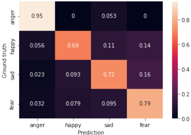</details> Once the training of our variational quantum circuits has converged, we measure our accuracy on the test dataset made of 180 sentences. We plot the results in the form of a normalized confusion matrix, comparing the ground truth and prediction. Figure 8: Normalized confusion matrix on the test dataset <details> <summary>Image 8 Details</summary>  ### Visual Description ## Heatmap: Emotion Prediction Accuracy ### Overview This heatmap visualizes the performance of an emotion classification model, showing the probability distribution of predicted emotions against ground truth labels. The matrix reveals model confidence in correctly identifying emotions and cross-prediction errors. ### Components/Axes - **Vertical Axis (Ground Truth)**: - Categories: anger, happy, sad, fear - **Horizontal Axis (Prediction)**: - Categories: anger, happy, sad, fear - **Color Legend**: - Scale: 0.0 (dark purple) to 0.8 (light yellow) - Position: Right side of the heatmap ### Detailed Analysis 1. **Anger (Ground Truth)**: - Predicted as anger: 0.95 (light yellow) - Predicted as happy: 0.00 - Predicted as sad: 0.053 (dark purple) - Predicted as fear: 0.00 2. **Happy (Ground Truth)**: - Predicted as anger: 0.056 (dark purple) - Predicted as happy: 0.69 (orange) - Predicted as sad: 0.11 (dark purple) - Predicted as fear: 0.14 (dark purple) 3. **Sad (Ground Truth)**: - Predicted as anger: 0.023 (dark purple) - Predicted as happy: 0.093 (dark purple) - Predicted as sad: 0.72 (orange) - Predicted as fear: 0.16 (dark purple) 4. **Fear (Ground Truth)**: - Predicted as anger: 0.032 (dark purple) - Predicted as happy: 0.079 (dark purple) - Predicted as sad: 0.095 (dark purple) - Predicted as fear: 0.79 (light yellow) ### Key Observations - **High Accuracy for Anger/Fear**: - Anger predictions show near-perfect accuracy (0.95) with minimal cross-prediction errors. - Fear predictions also demonstrate strong performance (0.79) but with slightly more confusion (0.095 for sad). - **Happy/Sad Confusion**: - Happy emotions are misclassified as fear (0.14) and sad (0.11) at similar rates. - Sad emotions are misclassified as fear (0.16) more frequently than happy (0.093). - **Model Bias**: - The diagonal dominance (correct predictions) suggests the model prioritizes anger and fear classifications. - Happy and sad emotions exhibit lower overall accuracy (0.69 and 0.72 respectively) with significant cross-prediction. ### Interpretation The model excels at identifying anger and fear, likely due to distinct features in training data for these emotions. However, happy and sad classifications suffer from lower accuracy and notable confusion between these two categories, suggesting overlapping emotional cues in the dataset. The near-zero values for anger predictions in non-anger categories indicate high confidence in anger detection, while the 0.053 sad prediction for anger suggests rare but notable misclassifications. This pattern highlights potential limitations in handling nuanced emotional states and opportunities for improving happy/sad differentiation through feature engineering or model refinement. </details> We reach satisfying accuracy results with an F1-score of 78%, with a confusion matrix concentrated on the diagonal. ## 5 Conclusion and prospects The DisCoCat model of meaning, by its structure and the computations it entails, seems to be an adequate way of tackling NLP problems on quantum machines. The potential scalability of the presented experiment bodes well for the future. The sentence length, the number of sentences and the vocabulary basis all grow linearly or sublinearly in the number of qubits. Running independent evaluations of quantum circuits on multiple quantum processors -if they become more accessible-, could be an adequate way of handling huge amount of sentences. With quantum processors of around 1000 qubits, performing NLP experiments on whole texts could be possible. In this paper, we have started to show the potential scalability of this method, realising for the first time a sentiment analysis with four emotions with a dataset of over 800 sentences. However, it is still important to remind that we are to this day still far from a quantum advantage. For the experiment presented in this paper, a simple TF-IDF feature extractor coupled with a Naive Bayes classifier reached 95% accuracy. This can be explained by the simplicity of the sentences used along with the small depth of the quantum circuits at hand. In a more general way, supervised learning can be directly linked to kernel methods, with the mapping to the higher dimensional Hilbert space corresponding to the encoding of the data on the quantum computer. For a quantum advantage to arise, the kernel linked to this higher dimensional mapping has to be hard to simulate classically, as shown by Schuld (2021). ## References Coecke, B., Sadrzadeh, M., and Clark, S. (2010). Mathematical foundations for a compositional distributional model of meaning. CoRR . Felice, G. D., Toumi, A., and Coecke, B. (2021). DisCoPy: Monoidal categories in python. Electronic Proceedings in Theoretical Computer Science , 333:183-197. Lorenz, R., Pearson, A., Meichanetzidis, K., Kartsaklis, D., and Coecke, B. (2021). QNLP in practice: Running compositional models of meaning on a quantum computer. CoRR . Nielsen, M. A. and Chuang, I. L. (2010). Quantum Computation and Quantum Information . Cambridge University Press. Schuld, M. (2021). Supervised quantum machine learning models are kernel methods.