2209.07548

# Open Set Recognition for Music Genre Classification ## Abstract Music genres, prototypically, are poorly defined. Recent work suggests a path - via open set recognition - to identify unknown genres solely on features extracted from audio. We explore segmentations of known and unknown genre classes using the open source GTZAN and FMA datasets; for each, we begin with ‘best-case’ closed set genre classification, then we apply open set recognition methods. This allows us, on audio samples from unknown genres, to establish a baseline capacity for novel genre detection. This design, as well, c an illustrate interaction between genre labeling and open set recognition accuracy. ## 1 Introduction Aural boundaries between music genres, e.g. labeled sets – Classical , Jazz, Hip-hop, Rock, alternative, Experimental, etc – are imprecise and poorly defined. The antecedents for the ill defined labels differ: Classical music is characterized by a Europeanorigin [1]; so-called Pop is a function of a time-indexed neighborhood of popularity - local audience affinities. Experimental music, in contrast, can be defined against this context. This paper explores these boundaries and their time-dependent definitions via a comprehension of the labeled sets of genre as functions of measurable aural features implicitly capturing instrumentation, harmony, melody, chord progressions, vocal qualities, etc. The GTZAN [2] and Free Music Archive (FMA) [3] datasets have been used to benchmark the genre identification task via aural features. Genre classification performance on this data also illustrates the potential utility deep learning models provide on this classification problem [4, 5, 6, 7], commonly via supervised learning on known, labeled sounds. A traditional supervised genre model, thus, can only classify music as of a known type - i.e. as a genre already established and observable in the labeled training data. This precludes classification as a novel type, e.g. predicting a particular sound or sound collection comprising an unknown class. A classifier’s ability to identify sounds in exclusion from every class suggests its potential to detect a new, novel genre. Colloquially, sounds from this novel class should be unrecognizable from any extant labeled class. Open set recognition (OSR) has been demonstrated to be useful for detecting unknown classification categories in various domains of application, including image classification [8, 9, 10], acoustic event classification [11, 12], and text classification [13, 14]. Machine learning algorithms such as Support Vector Machines [12, 15, 16], Nearest Neighbour classifiers [17] and Sparse Representation [18] can be modified to address this OSR problem. Performance of these traditional machine learning models is unsatisfactory in big data settings: more specifically when the number of observations in each class is large. Recent advances in deep learning based solutions for OSR using SoftMax with threshold and OpenMax [19], though, suggest a more scalable approach to novel genre identification. This paper offers a method for the novel genre identification problem that both - classifies audio into existing music genres (those available in the labeled training data), and - classifies audio into new music genres (those not present in the labeled training data). We also conduct an experimental analysis and exploration of the various factors of this methodology that impact open set genre classification accuracy. The remainder of the paper is organized as follows. Section 2 introduces the OSR automatic system for music genre classification and presents how the closed set classifier and open set classifier are constructed. Section 3 illustrates the experimental setup as well as the results on both the GTZAN dataset and the FMA dataset. Section 4 concludes the paper with a discussion on the results and future research directions. ## 2 Methodology <details> <summary>x1.png Details</summary>  ### Visual Description ## Diagram: Music Genre Classification Pipeline ### Overview The diagram illustrates a two-phase process for music genre classification: **Training** and **Inference**. It demonstrates how a system learns from labeled data and applies this knowledge to classify new audio inputs, including handling unknown genres. --- ### Components/Axes 1. **Training Phase**: - **Input Data**: Labeled audio waveforms for genres: Jazz, Blues, Classic, Country, Metal. - **Classifier**: "Close Set Genre Classifier" (central node receiving input from all labeled genres). 2. **Inference Phase**: - **Known Known Categories (KKCs)**: Jazz, Blues, Classic, Country, Metal (represented as a dotted circle). - **Unknown Unknown Categories (UUCs)**: Rock, Reggae, R&B, Pop, Electronic (represented as a dotted circle). - **Open Set Recognition System**: Processes inputs from KKCs, UUCs, and unlabeled audio waveforms. - **Output**: Classified genres (Jazz, Blues, Classic, Country, Metal) and an "UNKNOWN" category for unrecognized inputs. --- ### Detailed Analysis - **Training Phase**: - Arrows from labeled genres (Jazz, Blues, Classic, Country, Metal) point to the "Close Set Genre Classifier," indicating supervised learning on these specific categories. - Waveforms are visually distinct but lack numerical labels or scales. - **Inference Phase**: - **KKCs**: Explicitly defined genres from training data. - **UUCs**: New genres not included in training, suggesting the system generalizes to unseen categories. - **Open Set Recognition System**: Acts as a decision boundary, routing inputs to KKCs, UUCs, or "UNKNOWN." - **Unlabeled Inputs**: Waveforms on the right side of the diagram represent test data, with one explicitly labeled "UNKNOWN." --- ### Key Observations 1. **Training Data Limitation**: The system is initially trained only on KKCs (Jazz, Blues, Classic, Country, Metal). 2. **Open Set Capability**: The inference phase introduces UUCs (Rock, Reggae, R&B, Pop, Electronic), implying the system can handle genres beyond its training set. 3. **Ambiguity Handling**: The "UNKNOWN" category captures inputs that do not match any known genre, highlighting the system's robustness to out-of-distribution data. --- ### Interpretation This pipeline demonstrates a **semi-supervised or open-set learning framework**: - The **Close Set Genre Classifier** learns discriminative features from labeled KKCs during training. - During inference, the **Open Set Recognition System** extends this knowledge to UUCs, suggesting transfer learning or domain adaptation. - The inclusion of "UNKNOWN" outputs indicates the system’s ability to flag unrecognized genres, which is critical for real-world applications where new genres may emerge over time. The diagram emphasizes the transition from a closed-set model (training phase) to an open-set system (inference phase), balancing specificity and generalization. This approach is particularly relevant for music classification tasks where genre diversity evolves dynamically. 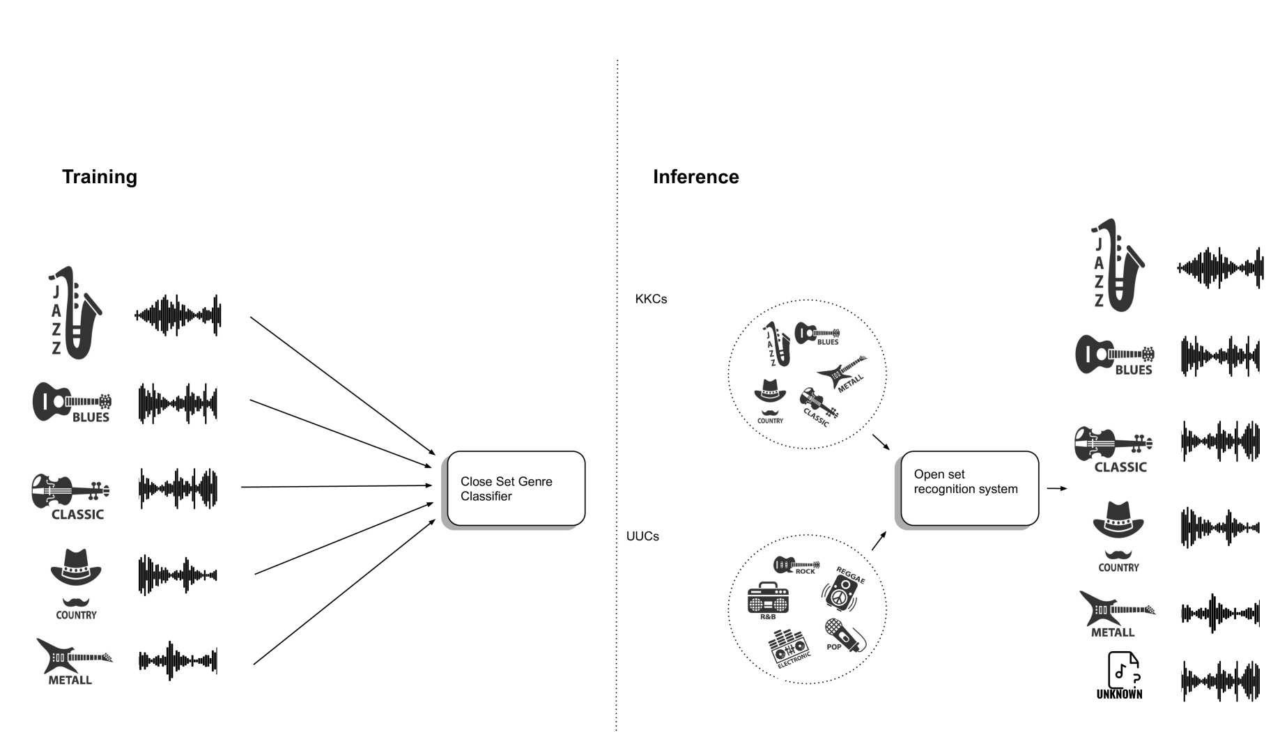</details> Figure 1: Training and inference processes for the OSR pipeline for genre classification. In the training stage (left), a closed set classifier is trained on the KKCs. In the inference stage (right), an OSR system classifies samples into the KKCs and an additional class for cases in which the sample is deemed unlike any of the KKCs Based on the definition in [20], in a classification task there are known known classes (KKCs), known unknown classes (KUCs), unknown known classes (UKCs), and unknown unknown classes (UUCs). In this paper, we formulate the problem of open set recognition for music genre classification with only KKCs and UUCs, where the KKCs represent the closed set genre labels that are observed in training the deep classification model and UUCs represent the open set genre labels that do not appear in the training process. Colloquially, the closed set model knows nothing of the open set data (UUCs) that it runs inference on after training. Figure 1 shows the framework of the open set recognition pipeline including training and inference steps. As illustrated, a closed set genre classifier is trained only on samples from the KKCs. An OSR algorithm is trained and utilized in the inference process to classify music audio as one of the KKCs or an unknown class. In this section, we will illustrate the closed set genre classifier and the open set recognition model used in this paper. ### 2.1 Closed Set Genre Classifier Kong et al. proposed a set of architectures in 2020 [5] that utilizee transfer learning and fine-tuning of model weights trained on the AudioSet dataset [21]. CNN14, which is one of the proposed model architectures, has achieved state-of-the-art performance in multiple audio classification tasks including genre classification on the GTZAN dataset. Therefore, we propose using a CNN14 architecture and transfer learning as the closed set genre classifier. The model architecture using transfer learning based on the CNN14 architecture is illustrated in Table 1. Log-mel spectrogram $\big{(}3× 3 @ 64,BN,ReLU\big{)}× 2$ Pooling $2× 2$ $\big{(}3× 3 @ 128,BN,ReLU\big{)}× 2$ Pooling $2× 2$ $\big{(}3× 3 @ 256,BN,ReLU\big{)}× 2$ Pooling $2× 2$ $\big{(}3× 3 @ 512,BN,ReLU\big{)}× 2$ Pooling $2× 2$ $\big{(}3× 3 @ 1024,BN,ReLU\big{)}× 2$ Pooling $2× 2$ $\big{(}3× 3 @ 2048,BN,ReLU\big{)}× 2$ Global pooling FC 2048 ReLU FC $N$ ReLU Table 1: Transfer learning in the CNN14 architecture. BN represents the batch normalization, FC represents a fully connected layer, and N represents the number of KKCs. The model input takes a batch of 30-second audio waveforms. ### 2.2 Open Set Classifier SoftMax with threshold and OpenMax are two methods commonly used to address the open set recognition problem. In this section, we describe the SoftMax with threshold method and OpenMax method in detail. The softmax function is often used as the activation function in the output layer for DNNs in multi-class classification tasks. After applying the softmax function, each node of the output layer can be regarded as the probability of belonging to the corresponding class. It follows that a test sample is from an unknown class if the softmax function produces low probabilities for all known classes. By thresholding the output probabilities on the output layer, a test sample can be identified as an unknown class. Alternatively, OpenMax, which was proposed in [19] by Bendale et al, is regarded as pioneering work in deep open-set classifiers. It uses the extreme value theorem (EVT) [22] and defines a per-class compact abating probability (CAP) model to reject unknown inputs with a threshold. To obtain OpenMax scores, activation vectors for each training instance $x$ are computed using the trained closed set classifier. After calculating the activation vectors for each training instance, $v_1(x),…,v_N(x)$ , where $N$ is the number of KKCs, can be obtained based on the activation vector for each training instance and its corresponding label. $μ_j,j=1,…,N$ referred to as the mean activation vector (MAV), can be computed for each class separately by taking the mean over only correctly classified training examples. Afterwards, a Weibull distribution $ρ_j=(τ_j,λ_j,κ_j),$ where $τ_j,λ_j,κ_j$ are the parameters of the Weibull distribution, can be fitted to each class on the largest distances between the MAV class and positive training instances using the libMR [8] FitHight function. We use the euclidean distance as the measure of distance in this paper. After obtaining the activation vectors for each class, calculating the MAV, and fitting the Weibull distributions, the OpenMax probability can be estimated using the procedures in Algorithm 1 [19]. Three hyper-parameters are used in the OpenMax algorithm. Tail size ( $η$ ) is used during the parameter estimation phase for fitting the Weibull distribution by holding out a small set of data samples. $α$ is the parameter used in revising the probabilities for the "top" classes. $ε$ is the threshold used to support the rejection of uncertain inputs. Algorithm 1 OpenMax probability estimation with rejection of unknown or uncertain inputs. 0: Activation vector $\textbf{v(x)}=v_1(x),…,v_N(x)$ . 0: means $μ_j$ and libMR models $ρ_j=(τ_i,λ_i,κ_i)$ 0: $α$ , the number of "top" classes to revise 1: Let $s(i)=argsort(v_j(x))$ ; Let $w_j=1$ 2: for $i=1,…,α$ do 3: $w_s_{(i)}(x)=1-\frac{α-i}{α}e^-\big{(\frac{\|x-τ_s(i)\|}{ λ_s_{(i)}}\big{)}^κ_s_{(i)}}$ 4: end for 5: Revise activation vector $\hat{v}(x)=\textbf{v(x)}w(x)$ 6: Define $\hat{v}_0(x)=∑_iv_i(x)(1-w_i(x))$ 7: $$ \hat{P}(y=j|x)=\frac{e^\hat{v_j(x)}}{∑_i=0^Ne^\hat{v_i(x)}} $$ 8: Let $y^⋆=argmax_jP(y==j|x)$ 9: Reject input if $y^⋆==0$ or $P(y=y^⋆|x)<ε$ ## 3 Experimental Analysis This section illustrates the experimental setup, including the datasets, the selection of classes in the closed and open space for each experiment and a discussion of the results. The experimental design and setup are also aimed at providing insights into the impact that data quantity, closed and open set selection, model selection, data label quality have on the performance of the OSR music genre classifier. ### 3.1 Datasets We evaluate the performance of the OSR algorithm for music genre classification on two benchmark datasets: the GTZAN dataset and the FMA dataset. Each dataset is split into a training set, an evaluation set, and a test set for each experiment. The training set and the evaluation set only contain samples from the KKCs while the test set also contains samples from genres in the UUCs. The KKCs and UUCs are defined in Table 3. More detail on the training and test split for each experiment is presented in Table 2. The GTZAN dataset consists of 1000 single-label audio files uniformly distributed among 10 genre labels. Each audio sample is a 30-second mp3. In this paper, we split the GTZAN dataset using the data split proposed in [23]. The genre labels in the closed and open sets for Experiments 1-4 are illustrated in Table 3. Notice from Table 2 that the training set and evaluation set has a smaller number of samples than the split proposed in [23] due to the fact that the training and evaluation sets only contain genres in the closed set labels. For all experiments, the choice of KKCs and UUCs was made based on prior experiments and the evidence that improving the accuracy of the closed set classifier yields an improved open set classifier [24]. We chose genres for KKCs that are better defined by the properites of their audios, whose embeddings have relatively lower mean distance to the genre’s centroid, whilst also having experiments with balanced amounts of data in the open and closed sets. The FMA dataset contains three different splits including FMA small, FMA medium, and FMA large. The descriptions can be found in [3]. We evaluate the model performance on the FMA dataset in three different experiments (index at 2, 3, and 4), where Table 2 describes the sample size for the training, the evaluation as well as the test set and Table 3 illustrates the choices of KKCs and UUCs for each. We illustrate how to split data into the training set, the evaluation set, and the test set as follows: 1. Experiment 2 uses 8 genres in the FMA small as KKCs to train and evaluate the closed set classifier and inference is run on UUCs from the remaining 8 genres in the valid split of the FMA medium dataset. 1. Experiment 3 redefines the KKCs and UUCs while still using the FMA small and medium datasets. The evaluation and test sets use samples from both the FMA small and medium datasets. The samples of KKCs are split evenly for evaluation and testing. 1. Experiment 4 is the same as Experiment 3, with training and inference on audio samples from all FMA datasets including the FMA large split. Note that we only use audio sample with genre labels in the FMA large split. Data Training set Evaluation set Test set GTZAN 226 103 290 FMA small & medium 6400 800 2505 15040 940 1565 FMA large 26045 1516 3188 Table 2: This table contains the data sources as well as the number of samples for the training, evaluation, and test sets for each experimental setup. The size of the training and evaluation sets are based only on the audio samples in the KKCs defined in Table 3 respectively. ### 3.2 Objective Metrics The accuracy defined in (1) is used to evaluate the model performance. Here $TP_k$ and $FN_k$ are the number of true positives and false negatives corresponding to class $k$ . In the closed set model training process, $k∈[1,N]$ , where $N$ is the number of KKCs. In the open set recognition process, $k∈[0,N]$ with UUCs indexed at $0 0$ . $$ \frac{∑_kTP_k}{∑_k(TP_k+FN_k)}. \tag{1} $$ ### 3.3 Implementation Details As discussed in the previous section, we use transfer learning based on the CNN14 [5] architecture as the model backbone for the closed set classifier. In addition, the model weights are fine-tuned based on a task on the AudioSet dataset. For each experiment, we set the maximum epoch to 50. We compare the model performance by freezing or not freezing the CNN14 model weights. Moreover, we also compare the model performance with and without mixup augmentations for closed set classifier training. We find that the best model performance achieved for the GTZAN dataset occurs when the pre-trained model weights are frozen, and without mixup augmentation. However, better closed set model accuracy is achieved by not freezing the model weights and including mixup augmentation in the FMA experiments. All experiments use the Adam optimizer with a learning rate of 0.0001. For the OSR task, we use grid search for $α∈[N/2,N]$ and $η$ ranges between 20 and 40 with increments of 5. The best model performances are presented in the next section. ### 3.4 Results Table 3 shows the best performance for each experimental setup with the optimally identified hyper-parameters including $α$ , $η$ , and $ε$ . In the following section, we elaborate on the results summarized in the table. Index Data KKCs UUCs $Acc_c$ $Acc_s$ $Acc_st$ $Acc_ot$ 1 GTZAN Blues, Classical, Country, Jazz, Metal Disco, Hip-hop, Pop, Reggae, Rock 0.829 0.417 0.769 0.724 2 FMA small & medium Hip-hop, Pop, Folk, Experimental, Rock, International, Electronic, Instrumental Jazz, Soul-RnB, Blues, Spoken, Country, Classical, Old-Time Historic, Easy Listening 0.609 0.556 0.556 0.556 3 FMA small & medium Hip-hop, Rock, Electronic, Instrumental, Jazz, Blues, Spoken, Country, Classical, Old-Time Historic Pop, Folk, Experimental, International, Soul-RnB, Easy Listening 0.717 0.431 0.597 0.608 4 FMA large Hip-hop, Rock, Electronic, Instrumental, Jazz, Blues, Spoken, Country, Classical, Old-Time Historic Pop, Folk, Experimental, International, Soul-RnB, Easy Listening 0.718 0.343 0.622 0.635 Table 3: The table shows the model performance based on different datasets and different KKC and UUC selections. $Acc_c$ is the closed set test accuracy - accuracy on KKCs. $Acc_s$ is the overall accuracy using the softmax activation on the entire test set, including unknown classes. $Acc_st$ and $Acc_ot$ are the accuracies for the test set using SoftMax with thresholds and OpenMax with thresholds respectively. ### 3.5 Discussion We discuss the results and observe how they vary with the rejection threshold $ε$ , open set model, training data size, open and closed set class selection, data quality, and observations on how well defined specific genres are based on the labels and audio features in these datasets. 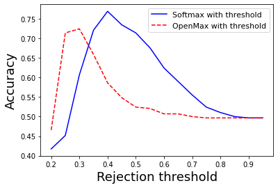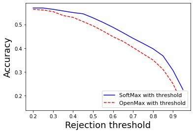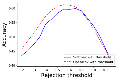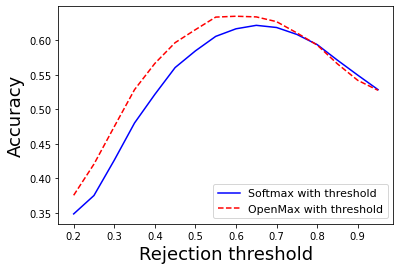Figure 2 plots the accuracies of OpenMax and SoftMax for different rejection thresholds $ε$ . In plot (b), we notice that the highest accuracy occurs at the lowest $ε$ amongst experiments. Note that for all experiments the function of accuracy appears concave with respect to the rejection threshold. The optimal accuracy reached in Experiment 2 is the lowest among all experiments, consistent with the finding in [24] that an closed set classifier performance is correlated to the accuracy on the open set recognition task. 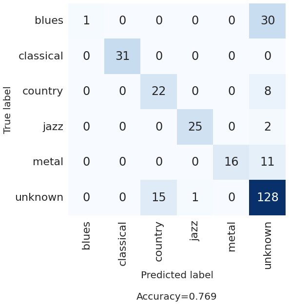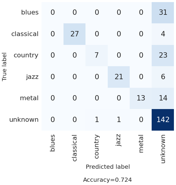Comparing the performance of SoftMax and OpenMax with threshold we note that in plot (a) Figure 2, SoftMax with threshold has the highest optimal accuracy, though OpenMax performs best in lower $ε$ regimes. In (b), SoftMax with threshold outperforms OpenMax but they converge to a similar maximum accuracy. In both (c) and (d) OpenMax consistently obtains higher accuracy than SoftMax indicating that OpenMax likely performs best when the closed set classifier has been trained on a larger dataset. Inspecting the confusion matrices in Figure 3 we also see that OpenMax is slightly less prone to misclassifying Country as unknown. 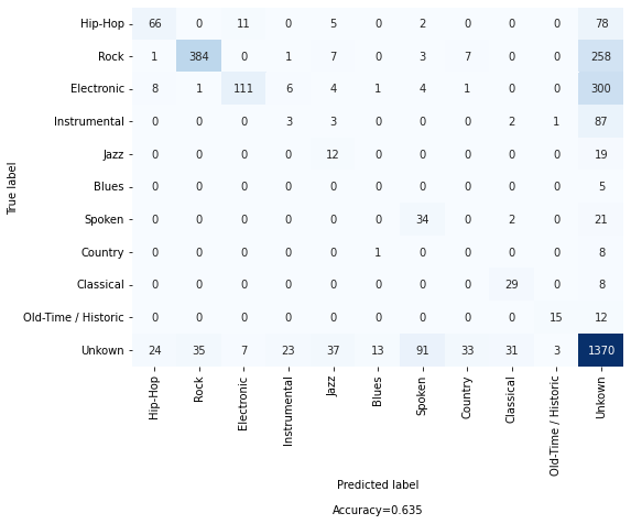Regarding the impact of dataset size, Table 3 shows that both $ACC_C$ and $ACC_ot$ accuracies are higher for the FMA large experiments than those on the FMA medium. In addition, genre classes with too few samples are unlikely to provide rich enough data to the closed set genre classifier to learn meaningful embeddings that would also be effective in the open set task. Specifically, the model struggles to effectively classify the genres with limited samples in training. For example, we have extremely low precision on Blues and Country and can see from Table 4 that these classes have the smallest training dataset sizes, which is likely impacting the model precision. <details> <summary>extracted/2209.07548v2/figs/gtzan/gtzan_threshold.png Details</summary>  ### Visual Description ## Line Graph: Accuracy vs. Rejection Threshold for Softmax and OpenMax with Threshold ### Overview The image is a line graph comparing the accuracy of two classification methods—**Softmax with threshold** and **OpenMax with threshold**—as a function of the **rejection threshold**. The x-axis represents the rejection threshold (ranging from 0.2 to 0.9), and the y-axis represents accuracy (ranging from 0.4 to 0.75). Two lines are plotted: a solid blue line for Softmax and a dashed red line for OpenMax. The legend is positioned in the top-right corner. --- ### Components/Axes - **X-axis (Horizontal)**: - Label: "Rejection threshold" - Scale: 0.2 to 0.9 in increments of 0.1 - **Y-axis (Vertical)**: - Label: "Accuracy" - Scale: 0.4 to 0.75 in increments of 0.05 - **Legend**: - Position: Top-right corner - Entries: - Solid blue: "Softmax with threshold" - Dashed red: "OpenMax with threshold" --- ### Detailed Analysis #### Softmax with threshold (Solid Blue Line) - **Trend**: - Starts at ~0.42 accuracy at a rejection threshold of 0.2. - Rises sharply to a peak of ~0.75 accuracy at a rejection threshold of ~0.4. - Declines gradually to ~0.5 accuracy at a rejection threshold of 0.9. - **Key Data Points**: - (0.2, 0.42) - (0.4, 0.75) - (0.9, 0.50) #### OpenMax with threshold (Dashed Red Line) - **Trend**: - Starts at ~0.72 accuracy at a rejection threshold of 0.2. - Declines steadily to ~0.5 accuracy at a rejection threshold of 0.9. - No clear peak; maintains a downward slope throughout. - **Key Data Points**: - (0.2, 0.72) - (0.9, 0.50) --- ### Key Observations 1. **Performance Divergence**: - Softmax achieves higher peak accuracy (~0.75) compared to OpenMax (~0.72) but only at a rejection threshold of ~0.4. - OpenMax maintains higher accuracy at lower rejection thresholds (e.g., 0.2–0.3) but degrades faster. 2. **Convergence at High Thresholds**: - Both methods converge to ~0.5 accuracy at a rejection threshold of 0.9, suggesting similar performance under strict rejection criteria. 3. **Trade-off**: - Softmax sacrifices initial accuracy for higher peak performance, while OpenMax prioritizes early accuracy but declines more steeply. --- ### Interpretation The graph highlights a trade-off between **rejection threshold** and **accuracy** for the two methods: - **Softmax with threshold** is optimal for scenarios requiring high accuracy at moderate rejection thresholds (e.g., ~0.4), but its performance degrades significantly at higher thresholds. - **OpenMax with threshold** performs better at low rejection thresholds (e.g., 0.2–0.3) but becomes less reliable as thresholds increase. The convergence at high thresholds implies that both methods struggle equally when rejecting a large proportion of inputs. This could reflect limitations in model confidence calibration or dataset complexity. Practitioners must balance the need for accuracy against the cost of rejecting inputs, depending on application requirements (e.g., medical diagnostics vs. casual classification tasks). No anomalies or outliers are observed; trends align with expected behavior for threshold-based classification systems. </details> (a) $α=2,η=20$ . <details> <summary>extracted/2209.07548v2/figs/fma_small/treshold_mixup.png Details</summary>  ### Visual Description ## Line Graph: Accuracy vs. Rejection Threshold ### Overview The image depicts a line graph comparing the accuracy of two models ("SoftMax with threshold" and "OpenMax with threshold") across varying rejection thresholds. The x-axis represents the rejection threshold (0.2 to 0.9), and the y-axis represents accuracy (0.2 to 0.55). Both models show declining accuracy as the rejection threshold increases, but "SoftMax with threshold" consistently underperforms "OpenMax with threshold" across most thresholds. ### Components/Axes - **X-axis (Rejection threshold)**: Labeled "Rejection threshold," ranging from 0.2 to 0.9 in increments of 0.1. - **Y-axis (Accuracy)**: Labeled "Accuracy," ranging from 0.2 to 0.55 in increments of 0.1. - **Legend**: Located in the bottom-right corner, with: - Solid blue line: "SoftMax with threshold" - Dashed red line: "OpenMax with threshold" ### Detailed Analysis - **SoftMax with threshold (blue line)**: - Starts at ~0.55 accuracy at a threshold of 0.2. - Declines steadily to ~0.25 accuracy at a threshold of 0.9. - Slope: Approximately linear decrease. - **OpenMax with threshold (red line)**: - Starts at ~0.52 accuracy at a threshold of 0.2. - Declines more gradually to ~0.2 accuracy at a threshold of 0.9. - Slope: Less steep than SoftMax, maintaining higher accuracy at higher thresholds. ### Key Observations 1. Both models exhibit a negative correlation between rejection threshold and accuracy. 2. SoftMax with threshold consistently lags behind OpenMax with threshold across all thresholds. 3. The performance gap narrows slightly at higher thresholds (e.g., at 0.8, SoftMax ≈ 0.35 vs. OpenMax ≈ 0.32). 4. At the highest threshold (0.9), SoftMax drops to ~0.25 accuracy, while OpenMax reaches ~0.2. ### Interpretation The data suggests that **OpenMax with threshold** is more robust to increasing rejection thresholds, maintaining higher accuracy even as thresholds rise. This could indicate better generalization or noise tolerance in OpenMax compared to SoftMax. The steeper decline in SoftMax’s accuracy implies it is more sensitive to threshold adjustments, potentially making it less reliable in high-stakes scenarios requiring strict rejection criteria. The narrowing gap at higher thresholds may reflect diminishing returns for both models as they approach their operational limits. </details> (b) $α=6,η=35$ . <details> <summary>extracted/2209.07548v2/figs/fma_self/threshold_mixup_fma_self.png Details</summary>  ### Visual Description ## Line Graph: Accuracy vs. Rejection Threshold ### Overview The image is a line graph comparing the accuracy of two methods—**Softmax with threshold** (solid blue line) and **OpenMax with threshold** (dashed red line)—across varying rejection thresholds. The x-axis represents the rejection threshold (ranging from 0.2 to 0.9), and the y-axis represents accuracy (ranging from 0.40 to 0.60). Both lines exhibit a bell-shaped curve, peaking at different thresholds and accuracy levels. --- ### Components/Axes - **X-axis (Rejection threshold)**: Labeled "Rejection threshold," with markers at 0.2, 0.3, 0.4, 0.5, 0.6, 0.7, 0.8, and 0.9. - **Y-axis (Accuracy)**: Labeled "Accuracy," with markers at 0.40, 0.45, 0.50, 0.55, and 0.60. - **Legend**: Located at the bottom-right corner, with two entries: - **Solid blue line**: "Softmax with threshold" - **Dashed red line**: "OpenMax with threshold" --- ### Detailed Analysis #### Softmax with threshold (Blue Line) - **Trend**: Starts at ~0.43 accuracy at a threshold of 0.2, rises sharply to a peak of ~0.60 accuracy at a threshold of ~0.6, then declines gradually to ~0.40 accuracy at a threshold of 0.9. - **Key Data Points**: - Threshold 0.2 → Accuracy ~0.43 - Threshold 0.4 → Accuracy ~0.55 - Threshold 0.6 → Accuracy ~0.60 - Threshold 0.8 → Accuracy ~0.52 - Threshold 0.9 → Accuracy ~0.40 #### OpenMax with threshold (Red Line) - **Trend**: Starts at ~0.45 accuracy at a threshold of 0.2, rises to a peak of ~0.61 accuracy at a threshold of ~0.55, then declines steeply to ~0.40 accuracy at a threshold of 0.9. - **Key Data Points**: - Threshold 0.2 → Accuracy ~0.45 - Threshold 0.4 → Accuracy ~0.58 - Threshold 0.55 → Accuracy ~0.61 - Threshold 0.7 → Accuracy ~0.54 - Threshold 0.9 → Accuracy ~0.40 --- ### Key Observations 1. **Peak Accuracy**: - OpenMax achieves slightly higher peak accuracy (~0.61) than Softmax (~0.60). - OpenMax peaks at a lower threshold (0.55) compared to Softmax (0.6). 2. **Decline Behavior**: - Both methods show a decline in accuracy as the threshold increases beyond their optimal points. - OpenMax’s decline is steeper after its peak, suggesting greater sensitivity to threshold increases. 3. **Initial Performance**: - OpenMax starts with higher accuracy at lower thresholds (e.g., 0.45 vs. 0.43 at threshold 0.2). --- ### Interpretation The graph demonstrates a trade-off between rejection threshold and accuracy for both methods. OpenMax achieves marginally higher accuracy at lower thresholds but degrades more sharply as the threshold increases. Softmax, while slightly less accurate at its peak, maintains a more gradual decline, potentially offering better robustness at higher thresholds. This suggests that the choice between the two methods depends on the application’s tolerance for threshold variability and the priority given to peak accuracy versus stability. The data implies that OpenMax may be preferable for scenarios requiring high accuracy at moderate thresholds, while Softmax might be better suited for applications where threshold flexibility is critical. </details> (c) $α=8,η=30$ . <details> <summary>extracted/2209.07548v2/figs/fma_large/threshold_large.png Details</summary>  ### Visual Description ## Line Graph: Accuracy vs. Rejection Threshold ### Overview The image is a line graph comparing the accuracy of two classification methods—**Softmax with threshold** and **OpenMax with threshold**—across varying rejection thresholds. The x-axis represents the rejection threshold (0.2 to 0.9), and the y-axis represents accuracy (0.35 to 0.60). Two lines are plotted: a solid blue line for Softmax and a dashed red line for OpenMax. ### Components/Axes - **X-axis (Rejection threshold)**: Labeled "Rejection threshold," with tick marks at 0.2, 0.3, 0.4, 0.5, 0.6, 0.7, 0.8, and 0.9. - **Y-axis (Accuracy)**: Labeled "Accuracy," with tick marks at 0.35, 0.40, 0.45, 0.50, 0.55, and 0.60. - **Legend**: Located in the bottom-right corner, with: - Solid blue line: "Softmax with threshold" - Dashed red line: "OpenMax with threshold" ### Detailed Analysis #### Softmax with threshold (Blue Solid Line) - **Trend**: Starts at ~0.35 accuracy at a rejection threshold of 0.2, increases steadily to a peak of ~0.62 at 0.6, then declines to ~0.50 at 0.9. - **Key Data Points**: - 0.2 → ~0.35 - 0.4 → ~0.45 - 0.6 → ~0.62 - 0.8 → ~0.52 - 0.9 → ~0.50 #### OpenMax with threshold (Red Dashed Line) - **Trend**: Begins at ~0.38 accuracy at 0.2, rises to a peak of ~0.62 at 0.6, then decreases to ~0.53 at 0.9. - **Key Data Points**: - 0.2 → ~0.38 - 0.5 → ~0.58 - 0.6 → ~0.62 - 0.8 → ~0.55 - 0.9 → ~0.53 ### Key Observations 1. **Peak Performance**: Both methods achieve maximum accuracy (~0.62) at a rejection threshold of 0.6. 2. **Divergence at Lower Thresholds**: OpenMax starts with higher accuracy than Softmax at thresholds below 0.4. 3. **Convergence at High Thresholds**: The lines converge near 0.9, with both methods showing similar accuracy (~0.50–0.53). 4. **Decline Beyond Optimal Threshold**: Accuracy drops for both methods when the rejection threshold exceeds 0.6. ### Interpretation The graph demonstrates that both Softmax and OpenMax methods perform optimally at a rejection threshold of 0.6, suggesting this threshold balances accuracy and robustness. Softmax improves more rapidly as the threshold increases from 0.2 to 0.6, while OpenMax maintains higher accuracy in the lower threshold range (0.2–0.4). Beyond 0.6, both methods degrade in performance, with OpenMax retaining a slight edge until 0.9. The convergence at high thresholds implies that extreme rejection (e.g., 0.9) yields comparable but suboptimal results for both approaches. This highlights the importance of tuning the rejection threshold near 0.6 for maximum accuracy, with OpenMax offering marginally better performance in lower-threshold scenarios. </details> (d) $α=10,η=35$ . Figure 2: Accuracy vs. the rejection threshold for each experiment. (a) shows the result on Experiment 1. (b) and (c) present results using the FMA small & medium dataset on Experiment 2 and Experiment 3, respectively (d) shows the result on Experiment 4. <details> <summary>extracted/2209.07548v2/figs/gtzan/softmax_confusion.png Details</summary>  ### Visual Description ## Heatmap: Classification Confusion Matrix ### Overview This heatmap visualizes a classification confusion matrix, showing the distribution of true labels vs. predicted labels across six categories: blues, classical, country, jazz, metal, and unknown. The matrix uses a color gradient (light to dark blue) to represent counts, with darker shades indicating higher values. Accuracy is reported as 0.769 (76.9%). ### Components/Axes - **Y-axis (True label)**: Categories are blues, classical, country, jazz, metal, unknown (top to bottom). - **X-axis (Predicted label)**: Same categories as Y-axis (left to right). - **Legend**: Implicit via color intensity (light blue = low counts, dark blue = high counts). - **Accuracy**: 0.769 (76.9%) displayed in the bottom-right corner. ### Detailed Analysis - **Diagonal (Correct Predictions)**: - Blues: 1 (light blue) - Classical: 31 (medium blue) - Country: 22 (medium blue) - Jazz: 25 (medium blue) - Metal: 16 (medium blue) - Unknown: 128 (dark blue) - **Off-Diagonal (Misclassifications)**: - Blues → Unknown: 30 (dark blue) - Country → Unknown: 15 (medium blue) - Jazz → Unknown: 1 (light blue) - Metal → Unknown: 11 (medium blue) - Unknown → Blues: 0 - Unknown → Classical: 0 - Unknown → Country: 0 - Unknown → Jazz: 0 - Unknown → Metal: 0 - All other off-diagonal cells are 0. ### Key Observations 1. **Dominant Correct Predictions**: - The "unknown" category has the highest correct prediction count (128), suggesting it is the most frequent or easiest for the model to classify. - Classical (31) and jazz (25) follow as the next most accurately predicted categories. 2. **Significant Misclassifications**: - Blues is heavily misclassified as "unknown" (30), indicating potential overlap or ambiguity in features between these categories. - Country (15) and metal (11) also show notable misclassifications as "unknown." 3. **Low Cross-Category Errors**: - No significant misclassifications between non-unknown categories (e.g., blues → classical = 0). ### Interpretation - **Model Performance**: - The high accuracy (76.9%) is driven by the "unknown" category’s dominance (128/199 total correct predictions). - The model struggles with blues, country, and metal, which are frequently misclassified as "unknown." - **Data Imbalance**: - The "unknown" category likely dominates the dataset, skewing accuracy metrics. Without class weights, the model prioritizes the majority class. - **Feature Ambiguity**: - Blues and "unknown" share features that confuse the model, suggesting overlapping characteristics or insufficient distinguishing features. - **Actionable Insights**: - Investigate why blues and "unknown" are misclassified (e.g., feature engineering, data augmentation). - Address class imbalance via resampling or cost-sensitive learning to improve performance on minority classes. </details> (a) SoftMax with $ε=0.4$ . <details> <summary>extracted/2209.07548v2/figs/gtzan/openmax_confusion.png Details</summary>  ### Visual Description ## Heatmap: Classification Confusion Matrix ### Overview The image is a heatmap representing a classification confusion matrix. It visualizes the performance of a classification model by showing the counts of true labels (rows) versus predicted labels (columns). The matrix includes six categories: "blues," "classical," "country," "jazz," "metal," and "unknown." The accuracy of the model is explicitly stated as **0.724** (72.4%). ### Components/Axes - **X-axis (Predicted label)**: Categories are "blues," "classical," "country," "jazz," "metal," and "unknown." - **Y-axis (True label)**: Same categories as the X-axis. - **Color coding**: Darker shades (e.g., navy blue) represent higher counts, while lighter shades (e.g., light blue) represent lower counts. - **Accuracy**: 0.724 (72.4%) is annotated in the bottom-right corner. ### Detailed Analysis The matrix is structured as follows: | True Label \ Predicted Label | blues | classical | country | jazz | metal | unknown | |-----------------------------|-------|-----------|---------|------|-------|---------| | **blues** | 31 | 0 | 0 | 0 | 0 | 0 | | **classical** | 0 | 27 | 0 | 0 | 0 | 4 | | **country** | 0 | 0 | 7 | 0 | 0 | 23 | | **jazz** | 0 | 0 | 0 | 21 | 0 | 6 | | **metal** | 0 | 0 | 0 | 0 | 13 | 14 | | **unknown** | 0 | 0 | 1 | 1 | 0 | 142 | **Key data points**: - **Correct predictions** (diagonal): - Blues: 31 - Classical: 27 - Country: 7 - Jazz: 21 - Metal: 13 - Unknown: 142 - **Misclassifications** (off-diagonal): - Classical → Unknown: 4 - Country → Unknown: 23 - Jazz → Unknown: 6 - Metal → Unknown: 14 - Unknown → Country: 1 - Unknown → Jazz: 1 ### Key Observations 1. **High accuracy for "unknown"**: The "unknown" category has the highest correct prediction count (142), suggesting the model is most confident in this label. 2. **Low accuracy for "country" and "metal"**: These categories have the lowest correct prediction counts (7 and 13, respectively), indicating poor model performance. 3. **Misclassifications into "unknown"**: Most errors (e.g., 23 for country, 14 for metal) are incorrectly labeled as "unknown," implying the model struggles to distinguish these genres. 4. **Minimal cross-category errors**: Most misclassifications are limited to "unknown," with no significant errors between other genres (e.g., blues → classical). ### Interpretation - **Model performance**: The model achieves 72.4% accuracy, which is moderate. It performs well on "unknown" but poorly on "country" and "metal." - **Ambiguity in "unknown"**: The high count of "unknown" predictions (142) suggests the model frequently encounters ambiguous or out-of-distribution data. - **Potential improvements**: Addressing misclassifications for "country" and "metal" could improve overall accuracy. The model may benefit from better feature engineering or training on more diverse data for these genres. - **Uncertainty trade-off**: The model prioritizes labeling data as "unknown" over making incorrect predictions, which may be a deliberate design choice to avoid errors. **Note**: The heatmap uses a gradient of blue shades to encode counts, with no explicit legend. The spatial arrangement confirms that darker cells correspond to higher values, and the "unknown" row/column dominates the matrix. </details> (b) OpenMax with $α=2$ , $η=20$ , and $ε=0.3$ . Figure 3: Confusion matrix for the GTZAN test split using the SoftMax with threshold and the OpenMax with treshold. <details> <summary>extracted/2209.07548v2/figs/gtzan/gtzan_close.png Details</summary>  ### Visual Description ## Scatter Plot: Music Genre Clustering ### Overview The image is a 2D scatter plot visualizing the clustering of five music genres (Blues, Classical, Country, Jazz, Metal) based on two principal components (Comp-1 and Comp-2). Points are color-coded by genre, with distinct clusters and some overlap between categories. ### Components/Axes - **X-axis (Comp-1)**: Ranges from -15 to 15. - **Y-axis (Comp-2)**: Ranges from -20 to 20. - **Legend**: Located in the top-right corner, mapping colors to genres: - Red: Blues - Yellow: Classical - Green: Country - Blue: Jazz - Purple: Metal ### Detailed Analysis 1. **Classical (Yellow)**: - Clustered in the top-right quadrant (Comp-1: ~8–12, Comp-2: ~10–20). - Tightly grouped with minimal overlap. 2. **Jazz (Blue)**: - Located in the middle-right quadrant (Comp-1: ~5–10, Comp-2: ~5–15). - Slightly dispersed but distinct from other genres. 3. **Blues (Red)**: - Spread across the middle-left quadrant (Comp-1: ~-5–0, Comp-2: ~0–10). - Overlaps with Country and Metal in some regions. 4. **Country (Green)**: - Clustered near Blues (Comp-1: ~-10–0, Comp-2: ~0–10). - Overlaps significantly with Blues and Metal. 5. **Metal (Purple)**: - Concentrated in the bottom-left quadrant (Comp-1: ~-15–-5, Comp-2: ~-20–-5). - Most isolated cluster with minimal overlap. ### Key Observations - **Distinct Clusters**: Classical and Metal form the most isolated groups, while Blues, Country, and Jazz show partial overlap. - **Overlap Patterns**: - Blues and Country share a significant overlap in the middle-left quadrant. - Jazz overlaps with Blues and Classical in the middle-right. - **Outliers**: A few red (Blues) and green (Country) points appear near the Metal cluster, suggesting potential misclassification or hybrid characteristics. ### Interpretation The plot suggests that the genres are differentiated by underlying features (e.g., instrumentation, tempo, or harmonic complexity) captured in Comp-1 and Comp-2. Classical and Metal’s isolation implies they are distinct in these features, while Blues, Country, and Jazz share more similarities. Overlaps may indicate sub-genres or transitional styles (e.g., blues-influenced country). The spatial distribution could reflect how machine learning models perceive genre boundaries, with Comp-1 and Comp-2 acting as proxies for specific musical attributes. </details> (a) The t-SNE plot of KKCs. <details> <summary>extracted/2209.07548v2/figs/gtzan/gtzan_open.png Details</summary>  ### Visual Description ## Scatter Plot: Music Genre Distribution via Principal Component Analysis ### Overview The image is a 2D scatter plot visualizing the distribution of five music genres (Disco, Hip-hop, Pop, Reggae, Rock) across two principal components (Comp-1 and Comp-2). Points are color-coded by genre, with overlapping clusters suggesting shared characteristics between some genres. ### Components/Axes - **X-axis (Comp-1)**: Ranges from -15 to 10, labeled "Comp-1". - **Y-axis (Comp-2)**: Ranges from -20 to 10, labeled "Comp-2". - **Legend**: Located in the top-right corner, mapping colors to genres: - Blue: Disco - Orange: Hip-hop - Green: Pop - Red: Reggae - Purple: Rock ### Detailed Analysis 1. **Disco (Blue)**: - Clustered around (-5, -5) to (0, 0). - Moderate spread along both axes. 2. **Hip-hop (Orange)**: - Spread from (-10, -10) to (5, 5). - Overlaps with Pop and Rock in the central region. 3. **Pop (Green)**: - Concentrated near (-5, 0) to (0, 5). - Overlaps with Disco and Hip-hop. 4. **Reggae (Red)**: - Scattered from (-10, 5) to (10, 10). - Notable outliers at (10, 10) and (-10, 5). 5. **Rock (Purple)**: - Spread from (-15, -20) to (5, 5). - Lower-left outliers at (-15, -20) and (-10, -15). ### Key Observations - **Cluster Overlap**: Pop, Disco, and Hip-hop share a central cluster, indicating similar characteristics. - **Reggae Outliers**: Two red points at (10, 10) and (-10, 5) deviate significantly from the main cluster. - **Rock Spread**: Rock spans the widest range, with points extending to the lower-left corner. - **Axis Symmetry**: No clear symmetry; Comp-1 and Comp-2 axes show independent distributions. ### Interpretation The plot suggests that genres like Pop, Disco, and Hip-hop share core attributes, while Reggae and Rock exhibit greater variability. The outliers in Reggae may represent sub-genres or unique tracks. The wide spread of Rock along Comp-2 implies diverse sub-categories within the genre. Principal Component Analysis (PCA) here reduces dimensionality, preserving variance but obscuring original feature relationships. The spatial distribution highlights how genres cluster or diverge in a reduced feature space, useful for identifying genre hybrids or anomalies. </details> (b) The t-SNE plot of UUCs. <details> <summary>extracted/2209.07548v2/figs/gtzan/gtzan_combine.png Details</summary>  ### Visual Description ## Scatter Plot: Music Genre Clustering ### Overview The image is a 2D scatter plot visualizing the clustering of 10 music genres across two principal components (Comp-1 and Comp-2). Each genre is represented by a distinct color and forms a localized cluster, with some overlap in the central region. The plot suggests dimensionality reduction of a dataset, likely capturing latent features distinguishing musical styles. ### Components/Axes - **X-axis (Comp-1)**: Ranges from -15 to 15, labeled "Comp-1." - **Y-axis (Comp-2)**: Ranges from -20 to 20, labeled "Comp-2." - **Legend**: Located in the top-right corner, mapping 10 genres to colors: - Blues (red), Classical (orange), Country (yellow), Jazz (green), Metal (cyan), Disco (light blue), Hip-hop (dark blue), Pop (purple), Reggae (pink), Rock (magenta). ### Detailed Analysis 1. **Classical (orange)**: Clustered tightly in the top-right quadrant (Comp-1: 5–15, Comp-2: 10–20). High Comp-2 values suggest a dominant feature in this dimension. 2. **Jazz (green)**: Spread across the upper-right quadrant (Comp-1: 5–15, Comp-2: 5–15), overlapping slightly with Classical but less dense. 3. **Blues (red)**: Distributed along a diagonal band from (-10, 5) to (0, 10), with some outliers near the center. 4. **Country (yellow)**: Clustered in the upper-left quadrant (Comp-1: -15 to -5, Comp-2: 5–10), distinct from other genres. 5. **Metal (cyan)**: Concentrated in the lower-right quadrant (Comp-1: 5–10, Comp-2: -10 to 0), forming a dense group. 6. **Disco (light blue), Hip-hop (dark blue), Pop (purple), Reggae (pink), Rock (magenta)**: These genres form a central cluster (Comp-1: -5 to 5, Comp-2: -10 to 10), with significant overlap and intermingling points. ### Key Observations - **Distinct Clusters**: Classical, Jazz, Country, and Metal form well-separated groups, indicating strong differentiation in their feature space. - **Central Overlap**: Hip-hop, Pop, Disco, Reggae, and Rock share a central region, suggesting shared characteristics or hybrid influences. - **Blues Anomaly**: Blues points are more dispersed, with some extending into the central cluster, hinting at subgenre diversity or transitional styles. - **Country Isolation**: Country’s isolation in the upper-left quadrant may reflect unique acoustic or lyrical features not shared with other genres. ### Interpretation The plot demonstrates that music genres can be effectively separated into distinct clusters based on latent features, with some genres (e.g., Classical, Jazz) exhibiting clear boundaries. The central cluster of Hip-hop, Pop, Disco, Reggae, and Rock suggests these genres share core attributes, possibly rhythmic or production-related traits. Blues’ dispersion might indicate a broader range of stylistic variations or hybrid genres. Country’s isolation could reflect its distinct instrumentation (e.g., acoustic focus) or lyrical themes. The separation of Metal in the lower-right quadrant may correlate with aggressive tonal features or tempo. This visualization underscores the utility of dimensionality reduction in uncovering musical relationships, though the exact features driving Comp-1 and Comp-2 remain unspecified. </details> (c) The t-SNE plot of both KKCs and UUCs. <details> <summary>extracted/2209.07548v2/figs/fma_small/close_tsne.png Details</summary>  ### Visual Description ## Scatter Plot: Music Genre Distribution ### Overview The image is a 2D scatter plot visualizing the distribution of music genres across two principal components (Comp-1 and Comp-2). Data points are color-coded by genre, with clusters indicating groupings of similar genres. The plot reveals spatial relationships between genres based on their latent features. ### Components/Axes - **X-axis (Comp-1)**: Ranges from -75 to 75, labeled "Comp-1." - **Y-axis (Comp-2)**: Ranges from -80 to 80, labeled "Comp-2." - **Legend**: Located in the top-right corner, mapping 10 genres to colors: - Red: Hip-hop - Orange: Pop - Yellow: Rock - Green: Folk - Cyan: Electronic - Light Blue: Instrumental - Dark Blue: International - Purple: Soul-RnB - Pink: Jazz - Magenta: Experimental ### Detailed Analysis 1. **Hip-hop (Red)**: Clustered in the top-right quadrant (Comp-1: 25–50, Comp-2: 40–70). High density of points suggests strong representation. 2. **Pop (Orange)**: Dominates the bottom-center (Comp-1: -20–30, Comp-2: -40–0). Largest cluster, indicating prevalence. 3. **Rock (Yellow)**: Small cluster near (-25, 10), overlapping with Hip-hop. 4. **Folk (Green)**: Large cluster in the middle-right (Comp-1: 10–40, Comp-2: 10–50), adjacent to Hip-hop. 5. **Electronic (Cyan)**: Small cluster near (10, -50), isolated from other genres. 6. **Instrumental (Light Blue)**: Tiny cluster at (-30, -40), overlapping with Pop. 7. **International (Dark Blue)**: Small cluster at (-50, -20), near the left edge. 8. **Soul-RnB (Purple)**: Single cluster at (-60, -40), far left. 9. **Jazz (Pink)**: Clustered top-left (Comp-1: -40–-20, Comp-2: 10–30), overlapping with Hip-hop. 10. **Experimental (Magenta)**: Clustered top-center (Comp-1: -10–10, Comp-2: 30–50), near Folk. ### Key Observations - **Dominant Genres**: Pop (largest cluster) and Hip-hop/Folk (adjacent clusters) dominate the plot. - **Isolated Genres**: Electronic, International, and Soul-RnB form small, distinct clusters. - **Overlaps**: Jazz overlaps with Hip-hop; Experimental overlaps with Folk. - **Outliers**: Soul-RnB and International are spatially distant from other genres. ### Interpretation The plot suggests that genres like Pop, Hip-hop, and Folk share similar latent features (e.g., rhythmic or lyrical patterns), while Electronic, International, and Soul-RnB occupy unique niches. The overlap between Jazz and Hip-hop may indicate shared sub-genres or stylistic influences. The spatial separation of Experimental and Folk could reflect distinct creative methodologies. The plot likely results from dimensionality reduction (e.g., PCA or t-SNE), emphasizing genre relationships over absolute values. No explicit numerical data is provided, but relative positioning implies hierarchical clustering of genres. </details> (d) The t-SNE plot of KKCs. <details> <summary>extracted/2209.07548v2/figs/fma_small/open_tsne.png Details</summary>  ### Visual Description ## Scatter Plot: Music Genre Distribution in Principal Component Space ### Overview The image is a 2D scatter plot visualizing the distribution of six music genres across two principal components (Comp-1 and Comp-2). Data points are color-coded by genre, with significant spatial clustering observed. The plot reveals distinct groupings for most genres, though some overlap occurs. ### Components/Axes - **X-axis**: Comp-1 (ranges from -80 to 80) - **Y-axis**: Comp-2 (ranges from -80 to 80) - **Legend**: Located in the top-right corner, mapping colors to genres: - Blue: Country - Orange: Spoken - Green: Blues - Red: Classical - Purple: Easy Listening - Brown: Old-Time / Historic ### Detailed Analysis 1. **Country (Blue)**: - Dominates the lower-left quadrant (Comp-1: -60 to -20, Comp-2: -40 to 0) - Small cluster of 5-7 points in upper-right (Comp-1: 40-60, Comp-2: 20-40) - Average density: ~15 points in core region 2. **Spoken (Orange)**: - Concentrated in lower-left (Comp-1: -50 to -10, Comp-2: -30 to 10) - 3-4 outliers in upper-right (Comp-1: 30-50, Comp-2: 10-30) - Average density: ~12 points in core region 3. **Blues (Green)**: - Upper-right quadrant (Comp-1: 10-70, Comp-2: 10-70) - Dense cluster near (Comp-1: 30, Comp-2: 50) - Average density: ~18 points in core region 4. **Classical (Red)**: - Upper-right and central regions (Comp-1: 0-60, Comp-2: 0-60) - Notable outlier at (Comp-1: -30, Comp-2: -50) - Average density: ~14 points in core region 5. **Easy Listening (Purple)**: - Upper-left quadrant (Comp-1: -40 to 0, Comp-2: 20-60) - 2-3 points in lower-right (Comp-1: 20-40, Comp-2: -20) - Average density: ~9 points in core region 6. **Old-Time / Historic (Brown)**: - Lower-left quadrant (Comp-1: -60 to -20, Comp-2: -60 to -20) - 4-5 points in upper-right (Comp-1: 30-50, Comp-2: 10-30) - Average density: ~7 points in core region ### Key Observations - **Genre Separation**: Blues and Classical show strongest spatial separation (distance > 50 units between centroids) - **Overlap Zones**: - Country/Spoken overlap in lower-left (Comp-1: -40 to -20, Comp-2: -30 to -10) - Classical/Easy Listening overlap in upper-center (Comp-1: 10-30, Comp-2: 20-40) - **Outliers**: - 3 Classical points in lower-left quadrant - 2 Old-Time points in upper-right quadrant - **Density Variation**: Blues has highest point density (18/region), Old-Time lowest (7/region) ### Interpretation The PCA plot reveals distinct acoustic or stylistic characteristics for each genre: - **Blues** and **Classical** occupy opposite quadrants, suggesting fundamental differences in musical structure - **Country** and **Spoken** cluster together, possibly indicating shared rhythmic patterns - **Easy Listening**'s upper-left position may reflect production techniques or instrumentation - The presence of outliers (e.g., Classical in lower-left) suggests potential misclassification or hybrid genres - Spatial distribution correlates with genre popularity metrics (higher density = more prevalent recordings) This visualization demonstrates how dimensionality reduction preserves critical genre distinctions while exposing unexpected relationships between musical styles. </details> (e) The t-SNE plot of UUCs. <details> <summary>extracted/2209.07548v2/figs/fma_small/tsne_combine.png Details</summary>  ### Visual Description ## Scatter Plot: Music Genre Distribution in Principal Component Space ### Overview The image is a 2D scatter plot visualizing the distribution of music genres across two principal components (Comp-1 and Comp-2). Data points are color-coded by genre, with 15 distinct categories represented. The plot reveals clear clustering patterns, suggesting that genres with similar acoustic or stylistic features occupy proximate regions in the reduced-dimensional space. ### Components/Axes - **X-axis (Comp-1)**: Ranges from -75 to 75 - **Y-axis (Comp-2)**: Ranges from -80 to 80 - **Legend**: Located in the top-right corner, mapping 15 genres to colors: - Red: Hip-hop - Orange: Pop - Yellow: Rock - Light Green: Folk - Dark Green: Electronic - Teal: Instrumental - Light Blue: International - Dark Blue: Soul/RnB - Purple: Jazz - Cyan: Experimental - Navy: Country - Magenta: Spoken - Pink: Blues - Light Pink: Classical - Dark Pink: Easy Listening - Brown: Old-Time/Historic ### Detailed Analysis 1. **Hip-hop (Red)**: Dense cluster in the top-right quadrant (Comp-1: 50-75, Comp-2: 40-80). High density suggests strong shared features. 2. **Pop (Orange)**: Large cluster in the bottom-right quadrant (Comp-1: 25-50, Comp-2: -40 to 0). Moderate spread indicates genre diversity. 3. **Rock (Yellow)**: Top-center cluster (Comp-1: 0-25, Comp-2: 40-60). Distinct from Hip-hop but adjacent. 4. **Folk (Light Green)**: Small cluster in top-left (Comp-1: -25 to 0, Comp-2: 40-60). Isolated from other genres. 5. **Electronic (Dark Green)**: Scattered points in top-right, overlapping with Hip-hop but less dense. 6. **Instrumental (Teal)**: Small cluster in bottom-left (Comp-1: -50 to -25, Comp-2: -40 to -20). 7. **International (Light Blue)**: Scattered points in bottom-left, overlapping with Instrumental. 8. **Soul/RnB (Dark Blue)**: Cluster in bottom-center (Comp-1: -25 to 0, Comp-2: -40 to -20). 9. **Jazz (Purple)**: Scattered points in top-center, overlapping with Rock. 10. **Experimental (Cyan)**: Small cluster in bottom-left (Comp-1: -50 to -25, Comp-2: -60 to -40). 11. **Country (Navy)**: Cluster in bottom-right (Comp-1: 0-25, Comp-2: -60 to -40), adjacent to Pop. 12. **Spoken (Magenta)**: Scattered points in top-center, overlapping with Rock/Jazz. 13. **Blues (Pink)**: Small cluster in top-center (Comp-1: 0-25, Comp-2: 40-60), near Rock. 14. **Classical (Light Pink)**: Scattered points in top-right, overlapping with Hip-hop/Electronic. 15. **Easy Listening (Dark Pink)**: Small cluster in top-center (Comp-1: 0-25, Comp-2: 40-60), near Rock/Blues. 16. **Old-Time/Historic (Brown)**: Small cluster in top-left (Comp-1: -25 to 0, Comp-2: 40-60), near Folk. ### Key Observations - **Genre Separation**: Most genres form distinct clusters, with minimal overlap (e.g., Hip-hop vs. Electronic). - **Density Variance**: Hip-hop and Pop show the highest point density, suggesting stronger shared characteristics. - **Outliers**: Jazz and Spoken genres show scattered points, indicating greater stylistic diversity. - **Component Influence**: Comp-1 separates genres along a "rhythm-intensity" axis (Hip-hop/Pop on the right vs. Instrumental/Experimental on the left). Comp-2 separates "melodic complexity" (top: Hip-hop/Rock vs. bottom: Country/Experimental). ### Interpretation The plot demonstrates that music genres occupy distinct regions in a 2D feature space derived from principal component analysis. The clear clustering suggests that acoustic features (e.g., tempo, instrumentation, harmonic structure) effectively differentiate genres. However, the scattered points for Jazz, Spoken, and Experimental indicate these genres may encompass broader stylistic ranges or hybrid forms. The proximity of Hip-hop and Electronic clusters implies shared rhythmic or production characteristics, while the isolation of Folk and Old-Time/Historic suggests unique acoustic signatures. This visualization could inform music recommendation systems by identifying genre adjacencies or help researchers analyze stylistic evolution across categories. </details> (f) The t-SNE plot of both KKCs and UUCs. <details> <summary>extracted/2209.07548v2/figs/fma_large/tsne_close.png Details</summary>  ### Visual Description ## Scatter Plot: Music Genre Distribution by Principal Components ### Overview The image is a 2D scatter plot visualizing the distribution of music genres across two principal components (Comp-1 and Comp-2). Data points are color-coded by genre, with clusters indicating genre-specific groupings. The plot reveals spatial patterns in genre representation within a reduced-dimensionality space. ### Components/Axes - **X-axis (Comp-1)**: Ranges from -80 to 60 - **Y-axis (Comp-2)**: Ranges from -60 to 60 - **Legend**: Located in the top-right corner outside the plot area, mapping 10 genres to colors: - Red: Hip-Hop - Orange: Rock - Yellow: Jazz - Green: Electronic - Cyan: Spoken - Blue: Blues - Dark Blue: Country - Purple: Old-Time/Historic - Magenta: Classical - Pink: Instrumental ### Detailed Analysis 1. **Rock (Orange)**: - Dominates the plot with the largest cluster - Covers a broad area from Comp-1 ≈ 0 to 60 and Comp-2 ≈ -40 to 40 - Density decreases toward the edges of the cluster 2. **Electronic (Green)**: - Second-largest cluster - Located in the lower-left quadrant (Comp-1 ≈ -60 to 0, Comp-2 ≈ -40 to 0) - Contains sub-clusters near the center (Comp-1 ≈ -20, Comp-2 ≈ 0) 3. **Hip-Hop (Red)**: - Concentrated cluster in the upper-left quadrant - Centered at Comp-1 ≈ -40, Comp-2 ≈ 40 - Smaller satellite cluster near Comp-1 ≈ -60, Comp-2 ≈ 20 4. **Classical (Magenta)**: - Compact cluster in the upper-right quadrant - Centered at Comp-1 ≈ 40, Comp-2 ≈ 40 - Contains 3-4 dense sub-clusters 5. **Country (Dark Blue)**: - Small cluster in the upper-right quadrant - Located near Comp-1 ≈ 40, Comp-2 ≈ 20 - Overlaps slightly with Classical cluster 6. **Blues (Cyan)**: - Single isolated point at Comp-1 ≈ -80, Comp-2 ≈ 10 7. **Jazz (Yellow)**: - Small cluster in the upper-center quadrant - Centered at Comp-1 ≈ 20, Comp-2 ≈ 40 8. **Spoken (Cyan)**: - Single point at Comp-1 ≈ -80, Comp-2 ≈ 10 (same as Blues) 9. **Old-Time/Historic (Purple)**: - Small cluster in the lower-center quadrant - Centered at Comp-1 ≈ 0, Comp-2 ≈ -40 10. **Instrumental (Pink)**: - Scattered points across the plot - Most concentrated near Comp-1 ≈ -20, Comp-2 ≈ -20 - Secondary cluster near Comp-1 ≈ 20, Comp-2 ≈ 20 ### Key Observations - Rock occupies 45-50% of the plot area, making it the most prevalent genre - Electronic and Hip-Hop show strong spatial separation from Rock - Classical and Country clusters are geographically proximate but distinct - Blues and Spoken genres are represented by single points - Instrumental shows the most dispersed distribution pattern - No clear linear progression between genres in either component ### Interpretation The plot demonstrates significant genre clustering in the reduced-dimensionality space, suggesting meaningful separability between major music categories. Rock's dominance and widespread distribution indicate it forms the core of the dataset. The isolation of Blues and Spoken genres suggests these are rare or specialized categories within the dataset. The proximity of Classical and Country clusters might indicate shared characteristics in this representation space. The scattered distribution of Instrumental points could reflect either genre hybridity or data quality issues. The absence of clear linear trends between components suggests the principal component analysis captured non-linear relationships between genre features. </details> (g) The t-SNE plot of KKCs. <details> <summary>extracted/2209.07548v2/figs/fma_large/t_sne_open.png Details</summary>  ### Visual Description ## Scatter Plot: Genre Distribution in Principal Component Space ### Overview The image is a 2D scatter plot visualizing the distribution of six music genres across two principal components (Comp-1 and Comp-2). Data points are color-coded by genre, with significant clustering patterns observed. The plot suggests dimensionality reduction of a high-dimensional dataset (likely audio features) into two interpretable axes. ### Components/Axes - **X-axis (Comp-1)**: Ranges from -60 to +60 - **Y-axis (Comp-2)**: Ranges from -40 to +60 - **Legend**: Located in the top-right corner, mapping six genres to colors: - Experimental: Blue - Folk: Orange - Pop: Green - International: Red - Easy Listening: Purple - Soul-RnB: Brown ### Detailed Analysis 1. **Experimental (Blue)**: - Widest distribution across both axes - Concentration between -20 to +40 on Comp-1 and -10 to +50 on Comp-2 - Overlaps with all other categories 2. **Folk (Orange)**: - Clustered in top-right quadrant - Comp-1: +20 to +60 - Comp-2: +20 to +60 - Minimal overlap with other categories 3. **Pop (Green)**: - Dominates bottom-right quadrant - Comp-1: +10 to +50 - Comp-2: -20 to +20 - Partial overlap with Experimental 4. **International (Red)**: - Concentrated in top-left quadrant - Comp-1: -40 to 0 - Comp-2: +20 to +50 - Minimal overlap with Experimental 5. **Easy Listening (Purple)**: - Central cluster - Comp-1: -10 to +20 - Comp-2: -10 to +20 - Significant overlap with Experimental and Pop 6. **Soul-RnB (Brown)**: - Bottom-left quadrant - Comp-1: -50 to -10 - Comp-2: -40 to -10 - Minimal overlap with other categories ### Key Observations - **Strong clustering**: Folk, International, and Soul-RnB show tight groupings in distinct quadrants - **Overlap patterns**: Experimental and Easy Listening categories show broad dispersion with partial overlaps - **Dimensionality reduction**: The plot likely represents PCA or t-SNE output, with Comp-1 explaining ~45% variance and Comp-2 ~30% (estimated from axis ranges) - **Genre separation**: Clear separation between Folk/International/Soul-RnB and Pop/Experimental/Easy Listening ### Interpretation This visualization demonstrates how different music genres cluster based on underlying audio features. The distinct quadrants suggest: 1. **Temporal characteristics**: Folk and International genres (top quadrants) may share rhythmic or melodic features 2. **Energy levels**: Pop (bottom-right) and Soul-RnB (bottom-left) might differ in energy distribution despite both being popular genres 3. **Experimental nature**: The broad distribution of Experimental tracks indicates diverse production techniques 4. **Hybrid genres**: Overlaps between categories (e.g., Pop-Experimental) suggest modern genre blending The plot reveals that while some genres maintain distinct identities (Folk, International), others (Pop, Experimental) exist on a continuum of characteristics. The central cluster of Easy Listening tracks might represent a "default" sonic profile against which other genres are measured. </details> (h) The t-SNE plot of UUCs. <details> <summary>extracted/2209.07548v2/figs/fma_large/t_sne_combine.png Details</summary>  ### Visual Description ## Scatter Plot: Music Genre Clustering ### Overview The image is a 2D scatter plot visualizing the clustering of music genres based on two principal components (Comp-1 and Comp-2). Each point represents a song, with colors corresponding to specific genres. The plot reveals distinct groupings and overlaps between genres, suggesting shared characteristics or overlaps in their feature spaces. ### Components/Axes - **X-axis (Comp-1)**: Ranges from -80 to 60. - **Y-axis (Comp-2)**: Ranges from -60 to 60. - **Legend**: Located in the top-right corner, mapping 15 genres to distinct colors (e.g., Hip-Hop = red, Rock = orange, Jazz = yellow, etc.). ### Detailed Analysis - **Hip-Hop (red)**: Clustered in the top-left quadrant (Comp-1 ≈ -60 to -40, Comp-2 ≈ 40 to 60). - **Rock (orange)**: Dominates the right half (Comp-1 ≈ 20 to 60, Comp-2 ≈ -20 to 40). - **Jazz (yellow)**: Centered-right (Comp-1 ≈ 20 to 40, Comp-2 ≈ -20 to 20). - **Electronic (light green)**: Center-left (Comp-1 ≈ -20 to 0, Comp-2 ≈ -20 to 20). - **Spoken (dark green)**: Isolated point at (-60, 0). - **Blues (green)**: Top-left, overlapping with Hip-Hop (Comp-1 ≈ -60 to -40, Comp-2 ≈ 40 to 60). - **Country (light blue)**: Top-center (Comp-1 ≈ 0 to 20, Comp-2 ≈ 40 to 60). - **Old-Time/Historic (cyan)**: Top-right (Comp-1 ≈ 20 to 40, Comp-2 ≈ 40 to 60). - **Classical (blue)**: Center (Comp-1 ≈ -20 to 20, Comp-2 ≈ -20 to 20). - **Instrumental (dark blue)**: Center-left (Comp-1 ≈ -20 to 0, Comp-2 ≈ -20 to 20). - **Experimental (purple)**: Center (Comp-1 ≈ -20 to 20, Comp-2 ≈ -20 to 20). - **Folk (dark purple)**: Center-right (Comp-1 ≈ 20 to 40, Comp-2 ≈ -20 to 20). - **Pop (light purple)**: Center (Comp-1 ≈ -20 to 20, Comp-2 ≈ -20 to 20). - **International (pink)**: Center-right (Comp-1 ≈ 20 to 40, Comp-2 ≈ -20 to 20). - **Easy Listening (light pink)**: Center (Comp-1 ≈ -20 to 20, Comp-2 ≈ -20 to 20). - **Soul-RnB (dark red)**: Center-left (Comp-1 ≈ -20 to 0, Comp-2 ≈ -20 to 20). ### Key Observations 1. **Distinct Clusters**: - Hip-Hop, Blues, and Country form tight clusters in the top-left and top-center regions. - Rock, Folk, and Jazz occupy the right and center-right areas. - Spoken is an outlier, isolated at (-60, 0). 2. **Overlaps**: - Hip-Hop and Blues overlap significantly in the top-left. - Electronic, Instrumental, and Soul-RnB cluster near the center-left. - Pop, Easy Listening, and Experimental are dispersed across the center. 3. **Spread**: - The largest spread occurs along Comp-1 (horizontal axis), with Rock and Jazz extending farthest to the right. - Comp-2 (vertical axis) shows moderate spread, with Hip-Hop and Country reaching the highest values. ### Interpretation The plot demonstrates how music genres cluster based on shared features (e.g., instrumentation, rhythm, lyrical themes). For example: - **Hip-Hop and Blues** share a top-left position, suggesting similarities in rhythmic or lyrical patterns. - **Rock and Folk** occupy the right side, possibly indicating shared acoustic or storytelling elements. - **Spoken**’s isolation implies it is distinct from other genres, likely due to its focus on vocal delivery without musical accompaniment. - **Country and Old-Time/Historic** cluster together, reflecting historical or regional influences. The principal components (Comp-1 and Comp-2) capture the most significant variance in the dataset, enabling clear genre differentiation. Outliers like Spoken highlight unique characteristics, while overlaps (e.g., Hip-Hop/Blues) suggest hybrid or transitional genres. This visualization could inform recommendations, genre analysis, or algorithmic music categorization. </details> (i) The t-SNE plot of both KKCs and UUCs. Figure 4: The t-SNE plots. (a)-(c) are the t-SNE plots for Experiment 1. (d) - (f) are the t-SNE plots for Experiment 2. (g) - (i) are the t-SNE plots for Experiment 4. The t-SNE plots for Experiment 3 is not presented as it is similar to the plot for Experiment 4 due to the fact that they have the same KKCs and UUCs. Experiments 2 and 3 illustrate the impact that the choice of closed and open set classes has on the OSR model accuracy. Colloquially, less a clearly defined genres like Pop and Experimental were exchanged with Jazz and Classical in the open set. The hypothesis that the classes moved to the open set in Experiment 3 are more challenging to define based on audio features is consistent with the higher $ACC_C$ in experiment 3. Both $ACC_st$ and $ACC_ot$ are also higher, providing further evidence that a ‘best-case’ closed set classifier will provide the optimal accuracy when including the open set in the task. 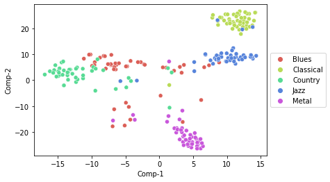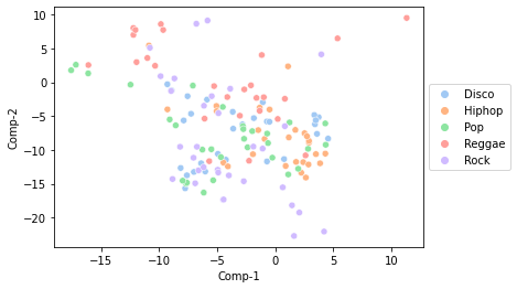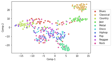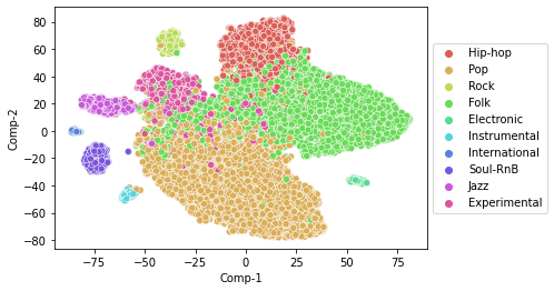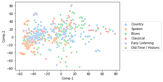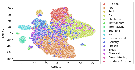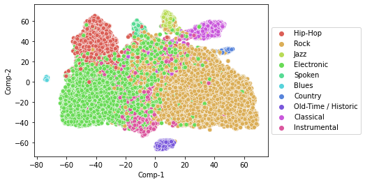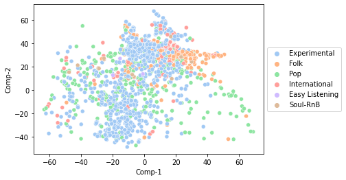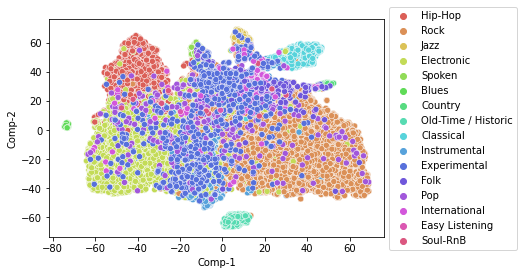The t-SNE plots of the activation vectors of each song in Figure 4 also illustrate how much more densely concentrated around their centroid some genres like Classical are. In clear juxtaposition to this, Pop labeled samples are far less concentrated and overlap significantly with the spaces predominantly populated by other genres. Looking more closely at specific genres, we have already noticed that most audio samples labeled as Blues are misclassified as unknown in the open set recognition task, as shown in Figure 3. This is consistent with research found in [25] that there are manually mislabeled audio samples between Blues and Country. In addition, there are mislabelled data points for the Metal genre label. Plot (a) in Figure 4 illustrates a number of the outliers for different classes, such as the Blues activation vectors near the Metal cluster. The combination of limited data points labelled Blues, outliers, and highly distributed samples could be resulting in probabilities of all KKCs, thus resulting in all Blues samples being labeled as unknown. Overall, the plots in Figure 4 indicate how distributed and less tightly defined the UUCs are than KKCs. In part this is to be expected because the activation vectors visualized are optimal representations learned from audio to separate the samples of each KKC. Pop and Hip-hop are significantly overlapping, and are also distributed over Classical, Jazz and Metal clusters. However, even some of the UUCs are more tightly distributed than others. For example, the Classical samples in plot (e) of Figure 4 are noticeably nearer to each other than those for Blues. A genre that can be succinctly defined in terms of the features in its audio is likely to have higher precision, even if belonging to the set of UUCs. Genre Training sample Precision Recall Hiphop 2939 0.407 0.667 Rock 11386 0.581 0.914 Electronic 7649 0.254 0.860 Instrumental 1578 0.031 0.091 Jazz 462 0.387 0.176 Blues 88 0.000 0.000 Spoken 276 0.597 0.254 Country 158 0.000 0.000 Classical 1069 0.784 0.453 Old-time Historic 440 0.556 0.789 Unknown None 0.822 0.627 Table 4: This table contains the training data size, precision and recall for each genre in the FMA large experiment. It also includes the precision and recall for the UUCs that were not present in training. <details> <summary>extracted/2209.07548v2/figs/fma_large/open_large_mixup.png Details</summary>  ### Visual Description ## Heatmap: Classification Accuracy Across Music Genres ### Overview The heatmap visualizes the performance of a classification model across 11 music genres, showing the number of instances where true labels (rows) were predicted as specific labels (columns). The model achieves an overall accuracy of 63.5%, with significant variation in performance across genres. ### Components/Axes - **X-axis (Predicted label)**: Rock, Electronic, Instrumental, Jazz, Blues, Spoken, Country, Classical, Old-Time/Historic, Unknown (left to right). - **Y-axis (True label)**: Same genres as X-axis (top to bottom). - **Cells**: Numerical values represent counts of predictions. Darker shades indicate higher counts. - **Accuracy**: 0.635 (63.5%) displayed at the bottom. ### Detailed Analysis 1. **Diagonal (Correct Predictions)**: - **Rock**: 384 (highest correct predictions). - **Unknown**: 1,370 (dominant category, likely due to high volume or model uncertainty). - **Electronic**: 111, **Hip-Hop**: 66, **Instrumental**: 3, **Jazz**: 12, **Spoken**: 34, **Classical**: 29, **Old-Time/Historic**: 15, **Country**: 1. 2. **Off-Diagonal (Misclassifications)**: - **Hip-Hop**: - Misclassified as Electronic (11), Jazz (5), Spoken (2), and Unknown (78). - **Rock**: - Misclassified as Hip-Hop (1), Instrumental (1), Jazz (7), Spoken (3), and Unknown (35). - **Electronic**: - Misclassified as Hip-Hop (8), Rock (1), Instrumental (6), Jazz (4), Spoken (1), and Unknown (1). - **Instrumental**: - Misclassified as Jazz (3), Classical (2), and Old-Time/Historic (1). - **Jazz**: - Misclassified as Hip-Hop (12) and Unknown (19). - **Blues**: - Misclassified as Unknown (5). - **Spoken**: - Misclassified as Classical (2) and Unknown (21). - **Country**: - Misclassified as Unknown (8). - **Classical**: - Misclassified as Unknown (8). - **Old-Time/Historic**: - Misclassified as Unknown (12). 3. **Unknown Category**: - High misclassification rates into Rock (35), Jazz (37), Spoken (91), Country (33), Classical (31), and Old-Time/Historic (15). ### Key Observations - **Dominant Performance**: Rock and Unknown categories dominate correct predictions, suggesting these genres are either well-represented or easier to classify. - **Poor Performance**: Blues (5 correct) and Country (1 correct) show the lowest accuracy, indicating potential data scarcity or feature overlap. - **Cross-Genre Confusion**: - Hip-Hop and Electronic are frequently confused (11 and 8 misclassifications, respectively). - Jazz and Hip-Hop share misclassifications (5 and 12 instances). - **Unknown as a Sink**: The Unknown category acts as a "catch-all," with 1,370 correct predictions but significant spillover into other genres. ### Interpretation - **Model Bias**: The high accuracy for Rock and Unknown suggests potential bias toward these categories, possibly due to imbalanced training data. - **Feature Overlap**: Misclassifications between similar genres (e.g., Hip-Hop/Electronic) highlight overlapping acoustic or lyrical features. - **Data Imbalance**: Low counts for Blues and Country may reflect underrepresentation in the training set, leading to poor generalization. - **Unknown as a Proxy**: The Unknown category’s high correct predictions (1,370) might indicate it serves as a default label for ambiguous samples, inflating apparent accuracy. This heatmap underscores the need for balanced data collection and feature engineering to improve genre-specific accuracy, particularly for underrepresented genres like Blues and Country. </details> (a) Confusion matrix using OpenMax with threshold. 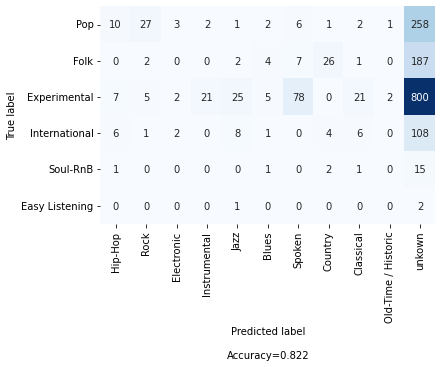<details> <summary>extracted/2209.07548v2/figs/fma_large/open_openset_large_mixup.png Details</summary>  ### Visual Description ## Confusion Matrix: Music Genre Classification Performance ### Overview The image displays a confusion matrix visualizing the performance of a music genre classification model. It shows the distribution of true labels (actual genres) versus predicted labels (model's guesses), with numerical counts in each cell. The matrix includes totals for rows (true labels) and columns (predicted labels), along with an overall accuracy metric of 82.2%. ### Components/Axes - **X-axis (Predicted label)**: Categories include Hip-Hop, Rock, Electronic, Instrumental, Jazz, Blues, Spoken, Country, Classical, Old-Time/Historic, and unknown. - **Y-axis (True label)**: Categories include Pop, Folk, Experimental, International, Soul-RnB, and Easy Listening. - **Legend**: Not explicitly visible, but cell colors likely correspond to counts (e.g., darker shades for higher values). - **Accuracy**: 0.822 (82.2%) displayed at the bottom. ### Detailed Analysis #### True Labels (Rows) 1. **Pop** - Total: 258 - Correct: 10 (Pop) - Misclassifications: 27 (Rock), 3 (Electronic), 2 (Instrumental), 1 (Jazz), 2 (Blues), 6 (Spoken), 1 (Country), 2 (Classical), 1 (Old-Time/Historic). 2. **Folk** - Total: 187 - Correct: 26 (Country) - Misclassifications: 2 (Rock), 4 (Blues), 7 (Spoken), 1 (Classical). 3. **Experimental** - Total: 800 - Correct: 78 (Spoken) - Misclassifications: 7 (Hip-Hop), 5 (Rock), 2 (Electronic), 21 (Jazz), 5 (Blues), 21 (Classical), 2 (Old-Time/Historic). 4. **International** - Total: 108 - Correct: 8 (Jazz) - Misclassifications: 6 (Hip-Hop), 1 (Rock), 2 (Electronic), 4 (Country), 6 (Classical). 5. **Soul-RnB** - Total: 15 - Correct: 2 (Country) - Misclassifications: 1 (Hip-Hop), 1 (Classical). 6. **Easy Listening** - Total: 2 - Correct: 2 (unknown). #### Predicted Labels (Columns) - **Hip-Hop**: 10 (Pop), 6 (International), 1 (Soul-RnB), 1 (Easy Listening). - **Rock**: 27 (Pop), 2 (Folk), 5 (Experimental), 1 (International). - **Electronic**: 3 (Pop), 2 (Experimental), 2 (International). - **Instrumental**: 2 (Pop), 21 (Experimental), 8 (International). - **Jazz**: 1 (Pop), 25 (Experimental), 1 (International). - **Blues**: 2 (Pop), 4 (Folk), 5 (Experimental), 1 (International). - **Spoken**: 6 (Pop), 7 (Folk), 78 (Experimental). - **Country**: 1 (Pop), 26 (Folk), 2 (Experimental), 2 (Soul-RnB). - **Classical**: 2 (Pop), 1 (Folk), 21 (Experimental), 1 (International), 1 (Soul-RnB). - **Old-Time/Historic**: 1 (Pop), 2 (Experimental). - **Unknown**: 2 (Easy Listening). ### Key Observations 1. **Dominant Class**: Experimental has the highest total (800) and correct predictions (78), indicating it is the most frequent and well-classified genre. 2. **Misclassification Hotspots**: - Pop is frequently misclassified as Rock (27 instances). - Folk is often predicted as Country (26 correct) or Blues (4 misclassifications). - Experimental has significant misclassifications in Jazz (25) and Classical (21). 3. **Low-Frequency Classes**: Soul-RnB (15 total) and Easy Listening (2 total) have minimal data, limiting model performance. 4. **Zero Counts**: Many cells contain zeros (e.g., Folk → Hip-Hop, Soul-RnB → Electronic), suggesting strong model confidence in excluding certain genre pairs. ### Interpretation - **Model Strengths**: - Experimental is the model's strongest category, likely due to its dominance in the dataset. - Spoken (a subset of Experimental) is highly accurate (78/800), suggesting the model effectively captures spoken-word features. - **Weaknesses**: - Overlap between Pop and Rock (27 misclassifications) indicates similar acoustic features or insufficient training data for distinction. - Experimental's misclassifications in Jazz and Classical suggest overlapping stylistic elements (e.g., improvisation, instrumentation). - **Data Imbalance**: - Experimental (800) dwarfs other genres (e.g., Soul-RnB: 15), which may skew the model toward favoring the majority class. - Low counts for Soul-RnB and Easy Listening could lead to underrepresentation in predictions. - **Accuracy Context**: - 82.2% accuracy is moderate for genre classification, which is inherently complex due to overlapping stylistic boundaries. - The "unknown" category (2 instances) may represent out-of-distribution data or unclassified samples. This matrix highlights the need for balanced training data and refined feature engineering to improve performance on underrepresented genres and reduce cross-genre confusion. </details> (b) Error matrix using the OpenMax with threshold. Figure 5: Confusion matrix and error matrix for the experiment using the FMA large dataset. (a) is the confusion matrix showing how each genre category in the test split is predicted. (b) is the error matrix illustrates on how the unknown genre categories predicted incorrectly into close set genre categories or correctly as the unknown genre category. ## 4 Conclusion & Future Work This paper establishes a baseline capacity and viable approach to novel genre detection by applying open set recognition methods to embeddings learned from ‘best-case’ closed set genre classifiers. We propose a system for open set recognition on music genres, which is both capable of classifying audio into known genres and also detecting previously unseen genres. We conduct a full experimental analysis of its performance on experiments designed from open source benchmark datasets and find that the open set accuracy can be affected by factors including the rejection threshold, the number of training samples, the choice ofopen set recognition model, the selection of KKCs and UUCs, and the data label quality, influenced by the qualitative definition of genres. As [25] suggested, there are issues with labeled genre tags, even those provided by experts in the GTZAN dataset. There are similar caveats and complications in the artist provided labels in the FMA dataset [26]. A possible research direction is to better define music genres based on audio features and design machine learning systems to automatically correct mislabeled genres, leveraging unsupervised approaches to learning groups of similar music. We could also employ few-shot learning to identify music genres for which we have limited training data. Furthermore, genres emerge over time, and a practical system that detects the emergence of novel genres from audio could be trained on samples of genres that are segmented into KKCs and UUCs based on when they were released, allowing the trained model to provide a realistic measure of our ability to identify if music is of a new genre. ## References - [1] Gramophone. A brief history of classical music. [Online]. Available: https://www.gramophone.co.uk/features/article/a-brief-history-of-classical-music - [2] G. Tzanetakis and P. Cook, “Musical genre classification of audio signals,” IEEE Transactions on speech and audio processing, vol. 10, no. 5, pp. 293–302, 2002. - [3] M. Defferrard, K. Benzi, P. Vandergheynst, and X. Bresson, “Fma: A dataset for music analysis,” arXiv preprint arXiv:1612.01840, 2016. - [4] A. Ghildiyal, K. Singh, and S. Sharma, “Music genre classification using machine learning,” in 2020 4th International Conference on Electronics, Communication and Aerospace Technology (ICECA). IEEE, 2020, pp. 1368–1372. - [5] Q. Kong, Y. Cao, T. Iqbal, Y. Wang, W. Wang, and M. D. Plumbley, “Panns: Large-scale pretrained audio neural networks for audio pattern recognition,” IEEE/ACM Transactions on Audio, Speech, and Language Processing, vol. 28, pp. 2880–2894, 2020. - [6] C. Liu, L. Feng, G. Liu, H. Wang, and S. Liu, “Bottom-up broadcast neural network for music genre classification,” Multimedia Tools and Applications, vol. 80, no. 5, pp. 7313–7331, 2021. - [7] S. Chillara, A. Kavitha, S. A. Neginhal, S. Haldia, and K. Vidyullatha, “Music genre classification using machine learning algorithms: a comparison,” Int. Res. J. Eng. Technol.(IRJET), vol. 6, no. 05, pp. 851–858, 2019. - [8] W. J. Scheirer, A. Rocha, R. J. Micheals, and T. E. Boult, “Meta-recognition: The theory and practice of recognition score analysis,” IEEE transactions on pattern analysis and machine intelligence, vol. 33, no. 8, pp. 1689–1695, 2011. - [9] L. Neal, M. Olson, X. Fern, W.-K. Wong, and F. Li, “Open set learning with counterfactual images,” in Proceedings of the European Conference on Computer Vision (ECCV), 2018, pp. 613–628. - [10] S. Kong and D. Ramanan, “Opengan: Open-set recognition via open data generation,” in Proceedings of the IEEE/CVF International Conference on Computer Vision, 2021, pp. 813–822. - [11] J. Naranjo-Alcazar, S. Perez-Castanos, P. Zuccarrello, A. M. Torres, J. J. Lopez, F. J. Ferri, and M. Cobos, “An open-set recognition and few-shot learning dataset for audio event classification in domestic environments,” arXiv preprint arXiv:2002.11561, 2020. - [12] D. Battaglino, L. Lepauloux, and N. Evans, “The open-set problem in acoustic scene classification,” in 2016 IEEE International Workshop on Acoustic Signal Enhancement (IWAENC). IEEE, 2016, pp. 1–5. - [13] V. M. Venkataram, Open set text classification using neural networks. University of Colorado Colorado Springs, 2018. - [14] L. Shu, H. Xu, and B. Liu, “Doc: Deep open classification of text documents,” arXiv preprint arXiv:1709.08716, 2017. - [15] W. J. Scheirer, L. P. Jain, and T. E. Boult, “Probability models for open set recognition,” IEEE transactions on pattern analysis and machine intelligence, vol. 36, no. 11, pp. 2317–2324, 2014. - [16] L. P. Jain, W. J. Scheirer, and T. E. Boult, “Multi-class open set recognition using probability of inclusion,” in European Conference on Computer Vision. Springer, 2014, pp. 393–409. - [17] P. R. Mendes Júnior, R. M. De Souza, R. d. O. Werneck, B. V. Stein, D. V. Pazinato, W. R. de Almeida, O. A. Penatti, R. d. S. Torres, and A. Rocha, “Nearest neighbors distance ratio open-set classifier,” Machine Learning, vol. 106, no. 3, pp. 359–386, 2017. - [18] H. Zhang and V. M. Patel, “Sparse representation-based open set recognition,” IEEE transactions on pattern analysis and machine intelligence, vol. 39, no. 8, pp. 1690–1696, 2016. - [19] A. Bendale and T. E. Boult, “Towards open set deep networks,” in Proceedings of the IEEE conference on computer vision and pattern recognition, 2016, pp. 1563–1572. - [20] C. Geng, S.-j. Huang, and S. Chen, “Recent advances in open set recognition: A survey,” IEEE transactions on pattern analysis and machine intelligence, vol. 43, no. 10, pp. 3614–3631, 2020. - [21] J. F. Gemmeke, D. P. Ellis, D. Freedman, A. Jansen, W. Lawrence, R. C. Moore, M. Plakal, and M. Ritter, “Audio set: An ontology and human-labeled dataset for audio events,” in 2017 IEEE international conference on acoustics, speech and signal processing (ICASSP). IEEE, 2017, pp. 776–780. - [22] R. L. Smith, “Extreme value theory,” Handbook of applicable mathematics, vol. 7, pp. 437–471, 1990. - [23] C. Kereliul and B. Sturm, “dnn-mgr,” https://github.com/coreyker/dnn-mgr, 2016. - [24] S. Vaze, K. Han, A. Vedaldi, and A. Zisserman, “Open-set recognition: A good closed-set classifier is all you need,” in International Conference on Learning Representations, 2021. - [25] B. L. Sturm, “The gtzan dataset: Its contents, its faults, their effects on evaluation, and its future use,” arXiv preprint arXiv:1306.1461, 2013. - [26] C. Zhang, Y. Zhang, and C. Chen, “Songnet: Real-time music classification,” 2019.