# Systematic KMTNet Planetary Anomaly Search, Paper VII: Complete Sample of $q < 10^{-4}$ Planets from the First Four-Year Survey
**Authors**: Weicheng Zang, Youn Kil Jung, Hongjing Yang, Xiangyu Zhang, Andrzej Udalski, Jennifer C. Yee, Andrew Gould, Shude Mao, Michael D. Albrow, Sun-Ju Chung, Cheongho Han, Kyu-Ha Hwang, Yoon-Hyun Ryu, In-Gu Shin, Yossi Shvartzvald, Sang-Mok Cha, Dong-Jin Kim, Hyoun-Woo Kim, Seung-Lee Kim, Chung-Uk Lee, Dong-Joo Lee, Yongseok Lee, Byeong-Gon Park, Richard W. Pogge, Przemek Mróz, Jan Skowron, Radoslaw Poleski, Michał K. Szymański, Igor Soszyński, Paweł Pietrukowicz, Szymon Kozłowski, Krzysztof Ulaczyk, Krzysztof A. Rybicki, Patryk Iwanek, Marcin Wrona, Mariusz Gromadzki, Hanyue Wang, Jiyuan Zhang, Wei Zhu
## Systematic KMTNet Planetary Anomaly Search, Paper VII: Complete Sample of q < 10 -4 Planets from the First Four-Year Survey
WEICHENG ZANG, 1,2 YOUN KIL JUNG, 3,4 HONGJING YANG, 1 XIANGYU ZHANG, 5 ANDRZEJ UDALSKI, 6 JENNIFER C. YEE, 2 ANDREW GOULD, 5,7 AND SHUDE MAO 1,8
(LEADING AUTHORS)
MICHAEL D. ALBROW, 9 SUN-JU CHUNG, 3,4 CHEONGHO HAN, 10 KYU-HA HWANG, 3 YOON-HYUN RYU, 3 IN-GU SHIN, 2 YOSSI SHVARTZVALD, 11 SANG-MOK CHA, 3,12 DONG-JIN KIM, 3 HYOUN-WOO KIM, 3 SEUNG-LEE KIM, 3,4 CHUNG-UK LEE, 3 DONG-JOO LEE, 3 YONGSEOK LEE, 3,12 BYEONG-GON PARK, 3,4 AND RICHARD W. POGGE 7 (THE KMTNET COLLABORATION)
PRZEMEK MR´ OZ, 6 JAN SKOWRON, 6 RADOSLAW POLESKI, 6 MICHAŁ K. SZYMA´ NSKI, 6 IGOR SOSZY ´ NSKI, 6 PAWEŁ PIETRUKOWICZ, 6 SZYMON KOZŁOWSKI, 6 KRZYSZTOF ULACZYK, 13 KRZYSZTOF A. RYBICKI, 6 PATRYK IWANEK, 6 MARCIN WRONA, 6 AND MARIUSZ GROMADZKI 6
(THE OGLE COLLABORATION)
HANYUE WANG, 2 JIYUAN ZHANG, 1 AND WEI ZHU 1 (THE MAP COLLABORATION)
1 Department of Astronomy, Tsinghua University, Beijing 100084, China
2 Center for Astrophysics | Harvard & Smithsonian, 60 Garden St.,Cambridge, MA 02138, USA
3 Korea Astronomy and Space Science Institute, Daejon 34055, Republic of Korea
4 University of Science and Technology, Korea, (UST), 217 Gajeong-ro Yuseong-gu, Daejeon 34113, Republic of Korea
Max-Planck-Institute for Astronomy, K¨ onigstuhl 17, 69117 Heidelberg, Germany
6 Astronomical Observatory, University of Warsaw, Al. Ujazdowskie 4, 00-478 Warszawa, Poland
7 Department of Astronomy, Ohio State University, 140 W. 18th Ave., Columbus, OH 43210, USA
8 National Astronomical Observatories, Chinese Academy of Sciences, Beijing 100101, China
9 University of Canterbury, Department of Physics and Astronomy, Private Bag 4800, Christchurch 8020, New Zealand
10 Department of Physics, Chungbuk National University, Cheongju 28644, Republic of Korea
11 Department of Particle Physics and Astrophysics, Weizmann Institute of Science, Rehovot 76100, Israel
12 School of Space Research, Kyung Hee University, Yongin, Kyeonggi 17104, Republic of Korea
13 Department of Physics, University of Warwick, Gibbet Hill Road, Coventry, CV4 7AL, UK
## ABSTRACT
We present the analysis of seven microlensing planetary events with planet/host mass ratios q < 10 -4 : KMT-2017-BLG-1194, KMT-2017-BLG-0428, KMT-2019-BLG-1806, KMT-2017-BLG-1003, KMT-2019BLG-1367, OGLE-2017-BLG-1806, and KMT-2016-BLG-1105. They were identified by applying the Korea Microlensing Telescope Network (KMTNet) AnomalyFinder algorithm to 2016-2019 KMTNet events. A Bayesian analysis indicates that all the lens systems consist of a cold super-Earth orbiting an M or K dwarf. Together with 17 previously published and three that will be published elsewhere, AnomalyFinder has found a total of 27 planets that have solutions with q < 10 -4 from 2016-2019 KMTNet events, which lays the foundation for the first statistical analysis of the planetary mass-ratio function based on KMTNet data. By reviewing the 27 planets, we find that the missing planetary caustics problem in the KMTNet planetary sample has been solved by AnomalyFinder. We also find a desert of high-magnification planetary signals ( A 65 ), and a follow-up project for KMTNet high-magnification events could detect at least two more q < 10 -4 planets per year and form an independent statistical sample.
1. INTRODUCTION
Among current exoplanet detection methods, a unique capability of the gravitational microlensing technique (Mao & Paczynski 1991; Gould & Loeb 1992) is to detect lowmass ( M planet 20 M ⊕ ) cold planets beyond the snow line (Hayashi 1981; Min et al. 2011), including Neptune-mass cold planets, which are common (Uranus and Neptune) in
our Solar System and cold terrestrial planets, which are absent in our Solar System. Because the typical host stars of the microlensing planetary systems are M and K dwarfs, detections of q < 10 -4 planets (where q is the planet/host mass ratio) can reveal the abundance of low-mass cold planets and answer how common the outer solar system is.
However, since the first microlensing planet, which was detected in 2003 (Bond et al. 2004), the first 13 years of microlensing planetary detections only discovered six q < 10 -4 planets 1 and none of them had mass ratios below 4 . 4 × 10 -5 . The paucity of detected q < 10 -4 planets led to important statistical implications for cold planets. Suzuki et al. (2016) analyzed 1474 microlensing events discovered by the Microlensing Observations in Astrophysics (MOA) survey (Sako et al. 2008) and formed a homogeneously selected sample including 22 planets. They found that the mass-ratio function of microlensing planets increases as q decreases until a break at q ∼ 1 . 7 × 10 -4 , below which the planetary occurrence rate likely drops. This break suggests that the Neptune-mass planets are likely to be the most common of cold planets. However, the Suzuki et al. (2016) sample only contains two q < 10 -4 and thus may be affected by small number statistics. To examine the existence of the break, a larger q < 10 -4 sample is needed.
After its commissioning season in 2015, the new-generation microlensing survey, the Korea Microlensing Telescope Network (KMTNet, Kim et al. 2016), has been conducting nearcontinuous, wide-area, high-cadence surveys for ∼ 96 deg 2 . The fields with cadences of Γ ≥ 2 hr -1 are the KMTNet prime fields ( ∼ 12 deg 2 ) and the other fields are the KMTNet sub-prime fields ( ∼ 84 deg 2 ). Since 2016, the detections of q < 10 -4 planets have been greatly increased in two ways, and the KMTNet data played a major or decisive role in all detections. First, more than ten q < 10 -4 planets have been detected from by-eye searches, including three with q < 2 × 10 -5 (Gould et al. 2020; Yee et al. 2021; Zang et al. 2021a). Second, Zang et al. (2021b, 2022a) developed the KMTNet AnomalyFinder algorithm to systematically search for planetary signals. This algorithm has been applied to the 2018 and 2019 KMTNet prime fields ( Γ ≥ 2 hr -1 ) and uncovered five new q < 10 -4 planets (Zang et al. 2021b; Hwang et al. 2022; Gould et al. 2022). Moreover, the systematic search opens a window for a homogeneous large-scale KMTNet planetary sample. According to the experience from 2018 and 2019 KMTNet prime fields, we expect to detect 20 planets with q < 10 -4 from 2016-2019 seasons.
1 They are OGLE-2005-BLG-169Lb (Gould et al. 2006), OGLE-2005BLG-390Lb (Beaulieu et al. 2006), OGLE-2007-BLG-368Lb (Sumi et al. 2010), MOA-2009-BLG-266Lb (Muraki et al. 2011), OGLE-2013-BLG0341Lb (Gould et al. 2014b), OGLE-2015-BLG-1670 (Ranc et al. 2019).
This will be an order of magnitude larger than the Suzuki et al. (2016) sample at q < 10 -4 .
To build the first KMTNet q < 10 -4 statistical sample, we applied the KMTNet AnomalyFinder algorithm to the 2016-2019 KMTNet microlensing events. In this paper, we introduce seven new q < 10 -4 events from this search. They are KMT-2017-BLG-1194, KMT-2017BLG-0428, KMT-2019-BLG-1806/OGLE-2019-BLG-1250, KMT-2017-BLG-1003, KMT-2019-BLG-1367, OGLE2017-BLG-1806/KMT-2017-BLG-1021, and KMT-2016BLG-1105. Together with 17 already published and three that will be published elsewhere, the KMTNet AnomalyFinder algorithm found 27 events that can be fit by q < 10 -4 models from 2016-2019 KMTNet data. However, whether a planet can be used for statistical studies requires further investigations, which is beyond the scope of this paper.
The paper is structured as follows. In Section 2, we briefly introduce the KMTNet AnomalyFinder algorithm and the procedure to form the q < 10 -4 sample. In Sections 3, 4 and 5, we present the observations and the analysis of seven q < 10 -4 events. Finally, we discuss the implications from the 2016-2019 KMTNet q < 10 -4 planetary sample in Section 6.
## 2. THE BASIC OF ANOMALYFINDER AND THE PROCEDURE
Section 2 of Zang et al. (2021b) and Section 2 of Zang et al. (2022a) together introduced the KMTNet AnomalyFinder algorithm. The AnomalyFinder uses a Gould (1996) 2dimensional grid of ( t 0 , t eff ) to search for and fit anomalies from the residuals to a point-source point-lens (PSPL, Paczy´ nski 1986) model. Here t 0 is the time of maximum magnification, and t eff is the effective timescale. For our search, the shortest t eff is 0.05 days and the longest t eff is 6.65 days. The parameters that evaluate the significance of a candidate anomaly are ∆ χ 2 0 and ∆ χ 2 flat . See Equation (4) of Zang et al. (2021b) for their definitions. The criteria of ∆ χ 2 0 and ∆ χ 2 flat are the same as the criteria used in Zang et al. (2022a); Gould et al. (2022); Jung et al. (2022), with ∆ χ 2 0 > 200 , or ∆ χ 2 0 > 120 and ∆ χ 2 flat > 60 for the KMTNet prime-field events and ∆ χ 2 0 > 100 , or ∆ χ 2 0 > 60 and ∆ χ 2 flat > 30 for the KMTNet sub-prime-field events. Future statistical studies should use the same criteria. In addition, an anomaly is required to contain at least three successive points ≥ 2 σ away from a PSPL model.
As a result, we found 464 and 608 candidate anomalies from 2016-2019 KMTNet prime-field and sub-prime-field events, respectively. We checked whether the data from other surveys are consistent with the KMTNet-based anomalies and cross-checked with C. Han's modeling. We fitted all the q < 10 -3 candidates with online data and found 13 new
candidates with q < 2 × 10 -4 . Then, we conducted tenderloving care (TLC) re-reductions and re-fitted the 13 events. Of these, eight events unambiguously have q < 10 -4 , three events, KMT-2016-BLG-1307, KMT-2017-BLG-0849, and KMT-2017-BLG-1057, have 10 -4 < q < 2 × 10 -4 , and two events, KMT-2016-BLG-0625 (Shin et al. in prep) and OGLE-2017-BLG-0448/KMT-2017-BLG-0090 (Zhai et al. in prep), have ambiguous mass ratios at 10 -5 q 10 -3 and will be published elsewhere.
Among the eight unambiguous q < 10 -4 events, one event, OGLE-2016-BLG-0007/MOA-2016-BLG-088/KMT2016-BLG-1991, will be published elsewhere because it has the lowestq of this sample. We analyze and publish the remaining seven events in this paper. We note that the planetary signals of the seven events are not strong, although they are confirmed by at least two data sets. We thus further check whether the light curves have other similar anomalies, to exclude the possibility of unknown systematic errors. We applied the AnomalyFinder algorithm to the re-reduction data. For all of the seven events, besides the known planetary signals no anomaly with ∆ χ 2 0 > 20 was detected. Therefore, the light curves of the seven events are stable and planetary signals are reliable.
## 3. OBSERVATIONS AND DATA REDUCTIONS
Table 1 lists the basic observational information for the seven events, including event names, the first discovery date, the coordinates in the equatorial and galactic systems, and the nominal cadences ( Γ ). The seven planetary events were all identified by the KMTNet post-season EventFinder algorithm (Kim et al. 2018a). Of them, KMT2019-BLG-1806/OGLE-2019-BLG-1250 and OGLE-2017BLG-1806/KMT-2017-BLG-1021 were discovered by the KMTNet alert-finder system (Kim et al. 2018b) and the Early Warning System (Udalski et al. 1994; Udalski 2003) of the Optical Gravitational Lensing Experiment (OGLE, Udalski et al. 2015), respectively, during their observational seasons. Hereafter, we designate KMT-2019-BLG-1806/OGLE2019-BLG-1250 and OGLE-2017-BLG-1806/KMT-2017BLG-1021 by their first-discovery name, KMT-2019-BLG1806 and OGLE-2017-BLG-1806. During the 2019 observational season, the KMTNet alert-finder system also discovered KMT-2019-BLG-1367. In addition, OGLE observed the locations of KMT-2019-BLG-1367 and KMT-2016-BLG1105 but did not alert them. We also include the OGLE data for these two events into the light-curve analysis, for which the OGLE data confirm the planetary signals found by the KMTNet. MOA did not issue alerts for any of the seven events, and there were no follow-up data to the best of our knowledge.
KMTNet conducted observations from three identical 1.6 m telescopes equipped with 4 deg 2 cameras in Chile
(KMTC), South Africa (KMTS), and Australia (KMTA). OGLE took data using an 1.3m telescope with 1.4 deg 2 field of view in Chile. For both surveys, most of the images were taken in the I band, and a fraction of V -band images were acquired for source color measurements. Each KMTNet Vband data point was taken one minute before or after one KMTNet I-band data point of the same field.
The KMTNet and OGLE data used in the light-curve analysis were reduced using the custom photometry pipelines based on the difference imaging technique (Tomaney & Crotts 1996; Alard & Lupton 1998): pySIS (Albrow et al. 2009, Yang et al. in prep) for the KMTNet data, and Wozniak (2000) for the OGLE data. For each event, the KMTC data were additionally reduced using the pyDIA photometry pipeline (Albrow 2017) to measure the source color. Except for OGLE-2017-BLG-1806 and KMT-2016-BLG-1105 whose sources are not located in any OGLE star catalog, the I -band magnitudes of the other five events reported in this paper have been calibrated to the standard I -band magnitude using the OGLE-III star catalog (Szyma´ nski et al. 2011).
## 4. LIGHT-CURVE ANALYSIS
## 4.1. Preamble
Because all seven events contain short-lived deviations from a PSPL model, we first introduce the common methods for the light-curve analysis. The PSPL model is described by three parameters, t 0 , u 0 , and t E , which respectively represent the time of lens-source closest approach, the closest lens-source projected separation normalized to the angular Einstein radius θ E , and the Einstein timescale,
<!-- formula-not-decoded -->
where κ ≡ 4 G c 2 au 8 . 144 mas M , M L is the lens mass, and ( π rel , µ rel ) are the lens-source relative (parallax, proper motion). In addition, for each data set i , we introduce two linear parameters, ( f S ,i , f B ,i ), to fit the flux of the source and any blend flux, respectively.
We search for binary-lens single-source (2L1S) models for each event. A 2L1S model requires four parameters in addition to the PSPL parameters, ( s, q, α, ρ ) , which respectively denote the planet-host projected separation in units of θ E , the planet/host mass ratio, the angle between the source trajectory and the binary axis, and the angular source radius θ ∗ scaled to θ E , i.e., ρ = θ ∗ /θ E .
Although the final results need detailed numerical analysis, some of the 2L1S parameters can be estimated by heuristic analysis. A PSPL fit excluding the data points around the anomaly can yield the three PSPL parameters, t 0 , u 0 , and t E . If an anomaly occurred at t anom , the corresponding lens-
Table 1. Event Names, Alerts, Locations, and Cadences for the six planetary events
| Event Name | Alert Date | RA J2000 | Decl . J2000 | | b | Γ(hr - 1 ) |
|--------------------|--------------|-------------|----------------|------------------|--------|--------------|
| KMT-2017-BLG-1194 | Post Season | 18:17:17.31 | - 25:19:26.18 | +6.63 | - 4.34 | 0.4 |
| KMT-2017-BLG-0428 | Post Season | 18:05:32.46 | - 28:29:25.01 | +2.59 | - 3.55 | 4 |
| KMT-2019-BLG-1806 | 26 Jul 2019 | 18:02:09.01 | - 29:24:53.60 | +1.41 | - 3.35 | 1 |
| OGLE-2019-BLG-1250 | | | | | | 0.3 |
| KMT-2017-BLG-1003 | Post Season | 17:41:38.76 | - 24:22:26.18 | +3.42 | +3.15 | 1 |
| KMT-2019-BLG-1367 | 27 Jun 2019 | 18:09:53.12 | - 29:45:43.96 | +1.93 | - 4.99 | 0.4 |
| OGLE-2017-BLG-1806 | 14 Oct 2017 | 17:46:29.58 | - 24:16:20.17 | +4.09 | +2.26 | 0.3 |
| KMT-2017-BLG-1021 | | | | | | 1 |
| KMT-2016-BLG-1105 | Post Season | 17:45:47.34 | - 26:15:58.93 | +2.30 | +1.16 | 1 |
source offset, u anom , and α can be estimated by
<!-- formula-not-decoded -->
Because the planetary caustics are located at the position of | s -s -1 | ∼ u anom , we obtain
<!-- formula-not-decoded -->
where s = s + and s = s -correspond to the major-image (quadrilateral) and the minor-image (triangular) planetary caustics, respectively. For two degenerate solutions with similar q but different s , Ryu et al. (2022) suggested that the geometric mean of two solutions satisfies
<!-- formula-not-decoded -->
In addition, Zhang et al. (2022) suggested a slightly different formalism, and Zhang & Gaudi (2022) provided a theoretical treatment of it. For a dip-type planetary signal, Hwang et al. (2022) pointed out that the mass ratio can be estimated by
<!-- formula-not-decoded -->
where ∆ t dip is the duration of the dip, and the accuracy of Equation (5) should be at a factor of ∼ 2 level.
To find all the possible 2L1S models, we conduct twophase grid searches for the parameters, ( log s , log q , α , ρ ). In the first phase, we conduct a sparse grid, which consists of 21 values equally spaced between -1 . 0 ≤ log s ≤ 1 . 0 , 20 values equally spaced between 0 ◦ ≤ α < 360 ◦ , 61 values equally spaced between -6 . 0 ≤ log q ≤ 0 . 0 and five values equally spaced between -3 . 5 ≤ log ρ ≤ -1 . 5 . We use a code based on the advanced contour integration code (Bozza 2010; Bozza et al. 2018), VBBinaryLensing 2 to compute the 2L1S magnification. For each grid point, we search for the minimum χ 2 by Markov chain Monte Carlo (MCMC) χ 2 minimization using the emcee ensemble sampler (Foreman-Mackey et al. 2013), with fixed ( log q , log s ) and free ( t 0 , u 0 , t E , ρ, α ). In the second phase, we conduct a denser ( log s , log q , α , ρ ) grid search around each local minimum (e.g., Zang et al. 2022b). Finally, we refine the best-fit models by MCMC with all parameters free.
For degenerate solutions, Yang et al. (2022) suggested that the phase-space factors can be used to weight the probability of each solution. We follow the procedures of Yang et al. (2022) and first calculate the covariance matrix, C , of ( log s, log q, α ) from the MCMC chain. Then, the phasespace factor is
<!-- formula-not-decoded -->
Because whether a planet and its individual solutions can be used for statistical studies requires further investigations, we provide the phase-space factors for the event with multiple solutions but do not use them to weight or reject solutions.
We also investigate whether the inclusion of two highorder effects can improve the fit. The first is the microlensing parallax effect (Gould 1992, 2000, 2004), which is due to the Earth's orbital acceleration around the Sun. We fit it by two parameters, π E , N and π E , E , which are the north and east components of the microlensing parallax vector π E in equatorial coordinates,
<!-- formula-not-decoded -->
2 http://www.fisica.unisa.it/GravitationAstrophysics/VBBinaryLensing. htm
Table 2. 2L1S Parameters for KMT-2017-BLG-1194
| Parameter | A | B |
|---------------|---------------------|---------------------|
| χ 2 /dof | 928.0/928 | 950.6/928 |
| t 0 ( HJD ′ ) | 7942 . 66 ± 0 . 13 | 7942 . 59 ± 0 . 13 |
| u 0 | 0 . 256 ± 0 . 018 | 0 . 246 ± 0 . 011 |
| t E (days) | 47 . 0 ± 2 . 5 | 47 . 9 ± 1 . 7 |
| ρ (10 - 3 ) | < 2 . 6 | < 1 . 4 |
| α (rad) | 2 . 505 ± 0 . 013 | 2 . 515 ± 0 . 011 |
| s | 0 . 8063 ± 0 . 0103 | 0 . 8055 ± 0 . 0065 |
| log q | - 4 . 582 ± 0 . 058 | - 4 . 585 ± 0 . 074 |
| I S , OGLE | 20 . 28 ± 0 . 08 | 20 . 34 ± 0 . 06 |
NOTE-The upper limit on ρ is 3 σ .
We also fit the u 0 > 0 and u 0 < 0 solutions to consider the 'ecliptic degeneracy' (Jiang et al. 2004; Poindexter et al. 2005). For four cases in this paper, the parallax contours take the form of elongated ellipses, so we report the constraints on the minor axes of the error ellipse, ( π E , ‖ ), which is approximately parallel with the direction of the Earth's acceleration. For the major axes of the parallax contours, π E , ⊥ ∼ π E , N , we only report it when the constraint is useful.
The second effect is the lens orbital motion effect (Batista et al. 2011; Skowron et al. 2011), and we fit it by the parameter γ = ( ds/dt s , dα dt ) , where ds/dt and dα/dt represent the instantaneous changes in the separation and orientation of the two components defined at t 0 , respectively. To exclude unbound systems, we restrict the MCMC trials to β < 1 . 0 . Here β is the absolute value of the ratio of projected kinetic to potential energy (An et al. 2002; Dong et al. 2009),
<!-- formula-not-decoded -->
and where π S is the source parallax estimated by the mean distance to red clump stars in the direction of each event (Nataf et al. 2013).
<!-- formula-not-decoded -->
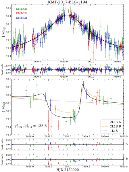
Figure 1 shows the observed data together with the best-fit PSPL and 2L1S models for KMT-2017-BLG-1194. There is a dip centered on HJD ′ ∼ 7958 . 9 (HJD ′ = HJD -2450000) , i.e., t anom ∼ 7958 . 9 , with a duration of ∆ t dip ∼ 1 . 05 days. The dip and the ridge around the dip are covered by three KMTNet sites, so the anomaly is secure. A PSPL fit yields ( t 0 , u 0 , t E ) = (7942.7, 0.26, 46), and using the heuristic formalism of Section 4.1, we obtain
<!-- formula-not-decoded -->
Figure 1. The observed data and the 2L1S (the black and orange solid lines) and 1L1S models (the grey dashed line) for KMT-2017BLG-1194. The data taken from different data sets are shown with different colors. The bottom panels show a close-up of the dip-type planetary signal and the residuals to the 2L1S models.
<details>
<summary>Image 1 Details</summary>
### Visual Description
\n
## Light Curve Analysis: KMT-2017-BLG-1194
### Overview
The image presents a light curve analysis of the variable star KMT-2017-BLG-1194. It consists of two main panels: a broader view of the light curve spanning a longer time period, and a zoomed-in view focusing on a specific event. Below each light curve are residual plots showing the difference between the observed data and the fitted model. The data is presented as magnitude (I-Mag) versus time (HJD-2450000).
### Components/Axes
* **Title:** KMT-2017-BLG-1194
* **X-axis (both panels):** HJD-2450000 (Heliocentric Julian Date - 2450000)
* **Y-axis (top panel & zoomed panel):** I-Mag (Magnitude in the I-band)
* **Y-axis (residual plots):** Residuals (difference between observed and modeled magnitude)
* **Legend (top panel):**
* KMTA31 (Green)
* KMTC31 (Blue)
* KMTS31 (Red)
* **Legend (zoomed panel):**
* 2LIS A (Black)
* 2LIS B (Orange)
* 1LIS (Purple)
* **Equation (zoomed panel):** χ<sup>2</sup><sub>LIS</sub> - χ<sup>2</sup><sub>2LIS</sub> = 135.6
### Detailed Analysis or Content Details
**Top Panel (Broad Light Curve):**
* The x-axis ranges from approximately 7920 to 7980 HJD-2450000.
* The y-axis ranges from approximately 18.2 to 19.4 I-Mag.
* The data points are scattered, with error bars indicating uncertainty.
* KMTA31 (Green): Data points show a general upward trend from approximately 19.2 I-Mag at 7920 HJD-2450000 to a peak around 18.3 I-Mag at 7940 HJD-2450000, then a decline to approximately 19.0 I-Mag at 7980 HJD-2450000.
* KMTC31 (Blue): Similar trend to KMTA31, but with more scatter. Starts around 19.3 I-Mag at 7920 HJD-2450000, peaks around 18.4 I-Mag at 7940 HJD-2450000, and ends around 19.1 I-Mag at 7980 HJD-2450000.
* KMTS31 (Red): Similar trend, but with even more scatter. Starts around 19.4 I-Mag at 7920 HJD-2450000, peaks around 18.5 I-Mag at 7940 HJD-2450000, and ends around 19.2 I-Mag at 7980 HJD-2450000.
* A black line represents a fitted model, generally following the upward and downward trends of the data. A blue line also represents a fitted model, but is flatter.
**Residual Plots (Top Panel):**
* The x-axis matches the top panel (7920 to 7980 HJD-2450000).
* The y-axis ranges from -0.25 to 0.25 for the residuals.
* Residuals for KMTA31 (Green), KMTC31 (Blue), and KMTS31 (Red) are plotted. The residuals appear randomly scattered around zero, indicating a reasonable fit of the model to the data.
**Bottom Panel (Zoomed Light Curve):**
* The x-axis ranges from approximately 7958.0 to 7960.5 HJD-2450000.
* The y-axis ranges from approximately 18.5 to 19.1 I-Mag.
* 2LIS A (Black): Shows a sharp peak around 7959.0 HJD-2450000, reaching approximately 18.6 I-Mag.
* 2LIS B (Orange): Shows a similar peak, but slightly less pronounced, around 7959.0 HJD-2450000, reaching approximately 18.7 I-Mag.
* 1LIS (Purple): Shows a broader peak around 7959.0 HJD-2450000, reaching approximately 18.8 I-Mag.
**Residual Plots (Bottom Panel):**
* The x-axis matches the zoomed panel (7958.0 to 7960.5 HJD-2450000).
* The y-axis ranges from -0.25 to 0.25 for the residuals.
* Residuals for 2LIS A (Black), 2LIS B (Orange), and 1LIS (Purple) are plotted. The residuals appear randomly scattered around zero, indicating a reasonable fit of the model to the data.
### Key Observations
* The broad light curve shows a clear microlensing event, with a peak around 7940 HJD-2450000.
* The zoomed light curve reveals a more detailed structure of the event, potentially indicating multiple peaks or a complex lens system.
* The residual plots suggest that the fitted models provide a good representation of the observed data.
* The χ<sup>2</sup> value indicates the quality of the fit. A lower value generally indicates a better fit.
### Interpretation
The image presents a light curve analysis of a microlensing event. Microlensing occurs when a massive object (like a star or black hole) passes between Earth and a distant source star, causing the source star to appear brighter. The shape of the light curve provides information about the mass and distance of the lensing object.
The two panels provide different levels of detail. The broad light curve shows the overall shape of the event, while the zoomed light curve reveals finer details. The residual plots confirm that the fitted models are consistent with the observed data.
The χ<sup>2</sup> value of 135.6 suggests a reasonable, but not necessarily perfect, fit of the models to the data. The difference between the χ<sup>2</sup> values for the 2LIS and 1LIS models suggests that the 2LIS model provides a better fit.
The presence of multiple peaks in the zoomed light curve could indicate a binary lens system, where two objects are acting as the lens. Further analysis would be needed to confirm this hypothesis. The different colors represent data from different telescopes (KMTA31, KMTC31, KMTS31), allowing for cross-validation and improved accuracy. The overall data suggests a complex microlensing event, potentially involving multiple lenses or a complex lens geometry.
</details>
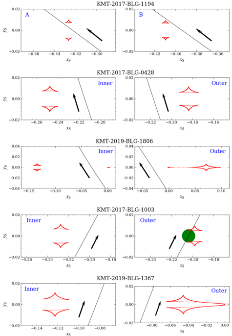
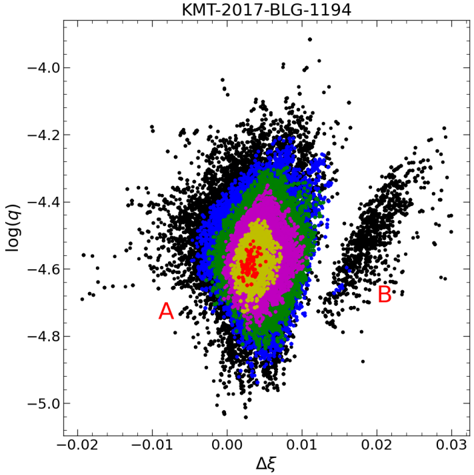
The grid search yields one solution. Its parameters are presented in Table 2 and are in good agreement with the heuristic estimates. The top left panel of Figure 2 displays the caustic structure and the source trajectory, for which the two minor-image planetary caustics are located on both sides of the source trajectory. We label the solution as the solution 'A'. To further investigate the parameter space and check whether the event has the inner/outer solutions (Gaudi & Gould 1997), for which the source passes inside (the 'Inner' solution) the two planetary caustics (closer to the central caustic) or outside (the 'Outer' solution), we follow the procedures of Hwang et al. (2018a). First, we conduct a 'hotter' MCMC with the error bar inflated by a factor of √ 3 . 0 . Second, we make a scatter plot of log q versus ∆ ξ from the 'hotter' MCMC chain. Here ∆ ξ represents the offset between the source and the planetary caustic as the source crosses the binary axis,
<!-- formula-not-decoded -->
The resulting scatter plot is shown in Figure 3, from which we find another local minimum at ∆ ξ ∼ 0 . 02 . We label this solution as the 'B' solution. As shown in the top right panel
<details>
<summary>Image 2 Details</summary>
### Visual Description
\n
## Charts: Microlensing Light Curves
### Overview
The image presents five individual microlensing light curves, each labeled with a unique identifier (KMT-2017-BLG-1194, KMT-2017-BLG-0428, KMT-2019-BLG-1806, KMT-2017-BLG-1003, and KMT-2019-BLG-1367). Each light curve plots the change in flux (y-axis, labeled as 'fs') against the relative source position (x-axis, labeled as 'xs'). Each plot contains red curves representing the light curve data, and black arrows indicating the direction of time evolution. Some plots also feature labeled regions ("Inner" and "Outer") and distinct data points (red triangles and a green circle).
### Components/Axes
* **x-axis:** Labeled 'xs', representing the relative source position. The scale varies for each plot, ranging approximately from -0.46 to 0.10.
* **y-axis:** Labeled 'fs', representing the flux. The scale varies for each plot, ranging approximately from -0.02 to 0.04.
* **Data Points:** Red curves represent the light curve data. Red triangles mark specific points on the curves. A single green circle is present in the KMT-2017-BLG-1003 plot.
* **Arrows:** Black arrows indicate the direction of time evolution along the light curve.
* **Labels:** Each plot is labeled with a unique identifier (e.g., KMT-2017-BLG-1194). The KMT-2017-BLG-0428, KMT-2019-BLG-1806, KMT-2017-BLG-1003, and KMT-2019-BLG-1367 plots also include "Inner" and "Outer" labels.
* **Sub-panels:** The image is divided into five sub-panels, each displaying a separate light curve.
### Detailed Analysis or Content Details
**KMT-2017-BLG-1194 (A & B):**
* Two subplots labeled A and B.
* The red curve in both plots slopes downward from left to right.
* Plot A: The curve starts at approximately (xs = -0.46, fs = 0.00) and ends at approximately (xs = -0.40, fs = -0.02). A red triangle is located at approximately (xs = -0.42, fs = 0.00).
* Plot B: The curve starts at approximately (xs = -0.42, fs = 0.00) and ends at approximately (xs = -0.38, fs = -0.02). A red triangle is located at approximately (xs = -0.40, fs = 0.00).
**KMT-2017-BLG-0428:**
* The red curve shows a peak.
* The curve starts at approximately (xs = -0.26, fs = 0.00) and reaches a peak at approximately (xs = -0.22, fs = 0.02), then decreases to approximately (xs = -0.16, fs = -0.02).
* A red triangle is located at approximately (xs = -0.24, fs = 0.00).
* The plot is labeled with "Inner" on the left side and "Outer" on the right side.
**KMT-2019-BLG-1806:**
* The red curve shows a complex shape with a dip and a rise.
* The curve starts at approximately (xs = -0.15, fs = 0.04) and decreases to approximately (xs = -0.05, fs = -0.04), then rises to approximately (xs = 0.10, fs = 0.00).
* A red triangle is located at approximately (xs = -0.10, fs = 0.00).
* The plot is labeled with "Inner" on the left side and "Outer" on the right side.
**KMT-2017-BLG-1003:**
* The red curve shows a peak.
* The curve starts at approximately (xs = -0.26, fs = 0.00) and reaches a peak at approximately (xs = -0.18, fs = 0.02), then decreases to approximately (xs = -0.24, fs = -0.02).
* A red triangle is located at approximately (xs = -0.24, fs = 0.00).
* A green circle is located at approximately (xs = -0.20, fs = 0.00).
* The plot is labeled with "Inner" on the left side and "Outer" on the right side.
**KMT-2019-BLG-1367:**
* The red curve shows a peak.
* The curve starts at approximately (xs = -0.14, fs = -0.02) and reaches a peak at approximately (xs = -0.08, fs = 0.02), then decreases to approximately (xs = -0.02, fs = -0.02).
* A red triangle is located at approximately (xs = -0.12, fs = 0.00).
* The plot is labeled with "Inner" on the left side and "Outer" on the right side.
### Key Observations
* All light curves exhibit a general downward trend, indicative of a microlensing event where the source star's brightness is being magnified and then diminished as a lensing object passes in front of it.
* The shapes of the curves vary, suggesting different lensing configurations (e.g., different lens masses, distances, and relative velocities).
* The presence of "Inner" and "Outer" labels in the last four plots suggests a division of the light curve based on the position of the lensing object relative to the source star.
* The green circle in KMT-2017-BLG-1003 represents a unique data point, potentially marking a specific feature of the lensing event (e.g., the peak magnification).
### Interpretation
These light curves represent observations of microlensing events, a phenomenon predicted by Einstein's theory of general relativity. Microlensing occurs when a massive object (the lens) passes between a distant source star and the observer (Earth), bending the light from the source and causing it to appear brighter. The shape and duration of the light curve provide information about the lens's mass, distance, and velocity.
The variations in the light curve shapes suggest that each event is caused by a different lensing configuration. The "Inner" and "Outer" labels likely delineate regions of the light curve corresponding to different phases of the lensing event. The green circle in KMT-2017-BLG-1003 could represent the point of maximum magnification or a specific feature related to the lens system.
The data suggests that these microlensing events are being used to study the distribution of compact objects (e.g., stars, planets, black holes) in the Milky Way galaxy. By analyzing the frequency and characteristics of these events, astronomers can infer the abundance and properties of these objects. The different identifiers (KMT-...) indicate that these observations were obtained by the Korea Microlensing Telescope Network.
</details>
Xs
Figure 2. Geometries of the five 'dip' planetary events. In each panel, the red lines represent the caustic, the black solid line represents the source trajectory, and the line with an arrow indicates the direction of the source motion. For the outer solution of KMT2017-BLG-1003, ρ is constrained at the > 3 σ level, so the radius of the green dot represents the source radius. For other solutions, ρ only has weak constraints with < 3 σ , so their source radii are not shown.
of Figure 2, the 'B' solution corresponds to the 'Inner' solution. Its parameters from MCMC are given in Table 2 and it is disfavored by ∆ χ 2 = 22 . 6 compared to the 'A' solution. In Figure 1, the 'B' solution cannot fit the anomaly well and all three KMTNet data sets contribute to the ∆ χ 2 . The ratio of the phase-space factors is p A : p B = 1 : 0 . 54 , which also prefers the 'A' solution. Thus, we exclude the 'B' solution. In addition, the models, which have the geometry of the 'Outer' solution, do not form a local minimum and are disfavored by ∆ χ 2 > 60 compared to the 'A' solution.
For the 'A' solution a point-source model is consistent within 1 σ and the 3 σ upper limit is ρ < 0 . 0026 . The inclusion of higher-order effects yields a constraint on π E , ‖ , and with the other 2L1S parameters being almost unchanged. We obtain π E , ‖ = -0 . 18 ± 0 . 35 and adopt the constraints on π E and ρ in the Bayesian analysis of Section 5. This is a new
Figure 3. Scatter plot of log q vs. ∆ ξ for KMT-2017-BLG-1194, where ∆ ξ = u 0 csc( α ) -( s -s -1 ) represents the offset between the source and the center of the planetary caustic at the moment that the source crosses the binary axis. The distribution is derived by inflating the error bars by a factor of √ 3 and then multiplying the resulting χ 2 by 3 for the plot. Red, yellow, magenta, green, blue and black colors represent ∆ χ 2 < 2 × (1 , 4 , 9 , 16 , 25 , ∞ ) . 'A' and 'B' represent two local minima and the corresponding parameters are given in Table 2.
<details>
<summary>Image 3 Details</summary>
### Visual Description
\n
## Scatter Plot: KMT-2017-BLG-1194
### Overview
The image presents a scatter plot displaying the relationship between Δξ (Delta Xi) and log(q). The plot appears to represent data from microlensing event KMT-2017-BLG-1194. The data points are densely clustered in a central region, with sparser points extending outwards, particularly towards the right. The plot uses color to indicate density of points. Two points, labeled 'A' and 'B', are highlighted in red.
### Components/Axes
* **Title:** KMT-2017-BLG-1194 (Top-center)
* **X-axis:** Δξ (Delta Xi) - Ranges approximately from -0.02 to 0.03.
* **Y-axis:** log(q) - Ranges approximately from -5.0 to -4.0.
* **Data Points:** Black dots representing individual data points.
* **Color Gradient:** A color gradient is used to represent the density of data points, ranging from dark blue (highest density) to green, pink/magenta, and finally to black (lowest density).
* **Labels:** 'A' and 'B' are red labels marking specific data points.
### Detailed Analysis
The data points are concentrated around Δξ ≈ 0. The density of points decreases as Δξ moves away from zero in either direction. The Y-axis, log(q), shows a wider distribution, with a concentration of points around log(q) ≈ -4.5.
* **Point A:** Located at approximately Δξ ≈ -0.005 and log(q) ≈ -4.7. It is within the high-density region (dark blue/green).
* **Point B:** Located at approximately Δξ ≈ 0.015 and log(q) ≈ -4.6. It is also within the high-density region (dark blue/green).
The color gradient indicates the following:
* **Dark Blue:** Highest density of points, centered around Δξ ≈ 0 and log(q) ≈ -4.5.
* **Green:** Medium-high density, surrounding the dark blue region.
* **Pink/Magenta:** Medium density, extending outwards from the green region.
* **Black:** Lowest density, representing sparse data points.
The data exhibits a roughly elliptical shape, elongated along the Δξ axis. The highest concentration of points forms a central, dense core.
### Key Observations
* The data is heavily concentrated around Δξ = 0, suggesting a strong preference for this value.
* The distribution of log(q) is broader, indicating a wider range of possible values.
* Points A and B are located within the high-density region, suggesting they are representative of the main population.
* The color gradient effectively visualizes the density of data points, highlighting the central concentration.
### Interpretation
This scatter plot likely represents the results of a microlensing event analysis. Δξ and log(q) are parameters related to the alignment and mass ratio of the lensing system. The concentration of points around Δξ = 0 suggests a near-perfect alignment between the source, lens, and observer. The distribution of log(q) provides information about the mass ratio of the lens and source stars.
The elliptical shape of the distribution could be due to observational biases or intrinsic properties of the lensing system. The highlighted points A and B may represent particularly interesting or significant data points within the event, potentially corresponding to specific features of the light curve. The color gradient is a useful tool for identifying regions of high and low data density, which can help to identify potential anomalies or outliers.
The plot demonstrates the characteristics of a microlensing event, where the bending of light from a distant source star by the gravity of a foreground lens star creates a temporary brightening of the source. The parameters Δξ and log(q) are crucial for characterizing the lensing event and inferring the properties of the lens star.
</details>
microlensing planet with q ∼ 2 . 62 × 10 -5 ; i.e., about nine times the Earth/Sun mass ratio.
## 4.2.2. KMT-2017-BLG-0428
Table 3. 2L1S Parameters for KMT-2017-BLG-0428
| Parameter | Inner | Outer |
|---------------|----------------------|----------------------|
| χ 2 /dof | 9952.0/9952 | 9952.1/9952 |
| t 0 ( HJD ′ ) | 7943 . 976 ± 0 . 030 | 7943 . 978 ± 0 . 031 |
| u 0 | 0 . 205 ± 0 . 009 | 0 . 205 ± 0 . 009 |
| t E (days) | 44 . 4 ± 1 . 5 | 44 . 3 ± 1 . 5 |
| ρ (10 - 3 ) | < 6 . 4 | < 6 . 1 |
| α (rad) | 1 . 890 ± 0 . 005 | 1 . 889 ± 0 . 005 |
| s | 0 . 8819 ± 0 . 0044 | 0 . 9146 ± 0 . 0050 |
| log q | - 4 . 295 ± 0 . 072 | - 4 . 302 ± 0 . 075 |
| I S , OGLE | 20 . 43 ± 0 . 05 | 20 . 43 ± 0 . 05 |
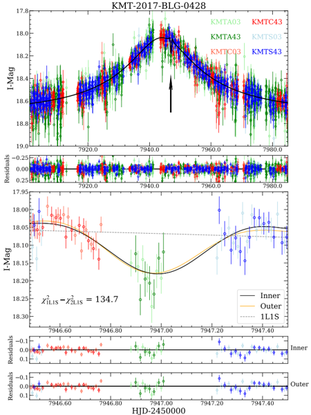
Figure 4 shows a ∆ I ∼ 0 . 12 mag dip at t anom ∼ 7947 . 00 , with a duration of ∆ t dip ∼ 0 . 74 days. The dip is defined by the KMTA and KMTC data, and the subtle ridges are sup-
Figure 4. The observed data and models for KMT-2017-BLG-0428. The symbols are similar to those in Figure 1. In the top panel, the black arrow indicates the position of the planetary signal.
<details>
<summary>Image 4 Details</summary>
### Visual Description
## Light Curve Analysis: KMT-2017-BLG-0428
### Overview
The image presents a light curve analysis of the microlensing event KMT-2017-BLG-0428. It consists of two main panels, each displaying a light curve with associated residuals. The top panel shows the full light curve, while the bottom panel focuses on a magnified section around the peak of the event. Error bars are present for each data point, indicating the uncertainty in the magnitude measurements.
### Components/Axes
* **Title:** KMT-2017-BLG-0428 (Top Center)
* **X-axis (both panels):** HJD-2450000 (Heliocentric Julian Date minus 2450000)
* Top Panel Range: Approximately 7920.0 to 7980.0
* Bottom Panel Range: Approximately 7946.60 to 7947.40
* **Y-axis (both panels):** I-Mag (Magnitude in the I-band)
* Top Panel Range: Approximately 17.8 to 19.0
* Bottom Panel Range: Approximately 18.05 to 18.25
* **Residuals Y-axis:** (Both panels) Range: Approximately -0.25 to 0.25
* **Legend (Top Panel, Top-Right):**
* KMTA03 (Red)
* KMTC43 (Blue)
* KMTA43 (Green)
* KMTS03 (Cyan)
* KMTS43 (Magenta)
* **Legend (Bottom Panel, Center-Right):**
* Inner (Black)
* Outer (Yellow)
* 1L1S (Brown)
* **Annotation (Top Panel, Center):** A black arrow pointing upwards, likely indicating the peak of the microlensing event.
* **Annotation (Bottom Panel, Center):** χ²<sub>LIS</sub> - χ²<sub>1L1S</sub> = 134.7
### Detailed Analysis or Content Details
**Top Panel:**
* **KMTA03 (Red):** The light curve shows a clear peak around HJD-2450000 = 7940.0, reaching a magnitude of approximately 18.0. Before and after the peak, the magnitude gradually increases to approximately 18.8.
* **KMTC43 (Blue):** Similar to KMTA03, this light curve exhibits a peak around HJD-2450000 = 7940.0, reaching a magnitude of approximately 18.1. The magnitude also increases to approximately 18.8 before and after the peak.
* **KMTA43 (Green):** This light curve shows a peak around HJD-2450000 = 7940.0, reaching a magnitude of approximately 18.3. The magnitude increases to approximately 18.9 before and after the peak.
* **KMTS03 (Cyan):** This light curve shows a peak around HJD-2450000 = 7940.0, reaching a magnitude of approximately 18.2. The magnitude increases to approximately 18.8 before and after the peak.
* **KMTS43 (Magenta):** This light curve shows a peak around HJD-2450000 = 7940.0, reaching a magnitude of approximately 18.1. The magnitude increases to approximately 18.8 before and after the peak.
* **Residuals (Bottom of Top Panel):** The residuals for all data series are scattered around zero, indicating a good fit of the model to the data.
**Bottom Panel:**
* **Inner (Black):** The light curve shows a peak around HJD-2450000 = 7946.9, reaching a magnitude of approximately 18.05.
* **Outer (Yellow):** The light curve shows a peak around HJD-2450000 = 7946.9, reaching a magnitude of approximately 18.15.
* **1L1S (Brown):** The light curve shows a peak around HJD-2450000 = 7946.9, reaching a magnitude of approximately 18.1.
* **Residuals (Bottom of Bottom Panel):** The residuals for all data series are scattered around zero, indicating a good fit of the model to the data.
### Key Observations
* All light curves show a similar peak shape, suggesting a common underlying event.
* The different telescopes (KMTA, KMTC, KMTS) provide consistent measurements.
* The residuals are generally small, indicating a good fit of the model to the data.
* The bottom panel provides a more detailed view of the peak, allowing for a more precise determination of the event parameters.
* The χ² value suggests a statistical comparison between different models (1L1S and Inner/Outer).
### Interpretation
The data represents a microlensing event, where the gravity of a foreground object bends and magnifies the light from a background star. The different light curves (KMTA03, KMTC43, etc.) are obtained from different telescopes observing the same event. The peak in the light curve corresponds to the maximum magnification, which occurs when the background star is closely aligned with the foreground object.
The bottom panel shows the best-fit model to the data, with the Inner, Outer, and 1L1S curves representing different possible configurations of the lensing system. The χ² value indicates that the 1L1S model provides a significantly better fit to the data than the Inner/Outer model. This suggests that the lensing event is likely caused by a single lens star (1L1S) rather than a binary lens system (Inner/Outer).
The residuals, which represent the difference between the observed data and the model predictions, are small and randomly distributed, indicating that the model accurately describes the observed data. The arrow in the top panel highlights the peak of the event, which is the most important feature of the light curve. The data suggests a well-characterized microlensing event with a single lens star.
</details>
ported by both the KMTC and KMTS data. These data were taken in good seeing ( 1 . ′′ 4 -2 . ′′ 5 ) and the anomaly does not correlate with seeing, sky background or airmass. In addition, Ishitani Silva et al. (2022) found that the KMTA data show systematic errors and excluded them from the analysis. In that case, the KMTA data exhibit similar residuals from one-night data in many places of the light curves. For the present case, the anomaly is mainly covered by the KMTA data, but as presented in Section 2, there is no similar deviation in other places of the light curves. We also carefully checked the KMTA data but did not find any similar residuals. Hence, the anomaly is secure. Applying the heuristic formalism of Section 4.1, we obtain
<!-- formula-not-decoded -->
The 2L1S modeling yields two degenerate solutions with ∆ χ 2 = 0 . 1 . As shown in Figure 2, the two solutions are subjected to the inner/outer degeneracy. Their parameters are given in Table 3, for which α and q are consistent with Equation (11). For s , we note that the geometric mean of the two solutions, s mean = 0 . 898 ± 0 . 005 , is in good agreement with Equation (11) and thus the formalism of Ryu et al. (2022). In addition, the observed data only provide a 3 σ upper limit on ρ , and a point-source model is consistent within 1 σ . The ratio of the phase-space factors is p inner : p outer = 0 . 78 : 1 .
With high-order effects, we find that the χ 2 improvement is ∼ 3 and other parameters are almost the same. The constraint of π E , π E , ‖ = -0 . 35 ± 0 . 26 , will be used in the Bayesian analysis. This is a microlensing planet with a Neptune/Sun mass ratio.
## 4.2.3. KMT-2019-BLG-1806
Figure 5. The observed data and models for KMT-2019-BLG-1806. The symbols are similar to those in Figure 1. In the top panel, the black arrow indicates the position of the planetary signal.
<details>
<summary>Image 5 Details</summary>
### Visual Description
\n
## Light Curve Analysis: Eclipsing Binary Star System
### Overview
The image presents a light curve analysis of an eclipsing binary star system, displaying brightness (I-Mag) variations over time (HJD-2450000). It consists of two main panels, each with a light curve and corresponding residuals plot. The data is presented for four different observing sources: KMTA04, KMTC04, KMTS04, and OGLE. A chi-squared value comparison is also provided.
### Components/Axes
* **X-axis (both panels):** HJD-2450000 (Heliocentric Julian Date minus 2450000). Scale ranges from approximately 8680.0 to 8760.0 in the top panel and 8717.4 to 8718.2 in the bottom panel.
* **Y-axis (top panel):** I-Mag (Instrumental Magnitude). Scale ranges from approximately 17.3 to 19.2.
* **Y-axis (bottom panel):** I-Mag (Instrumental Magnitude). Scale ranges from approximately 17.35 to 17.6.
* **Y-axis (Residuals plots):** Residuals. Scale ranges from approximately -0.25 to 0.25 (top panel) and -0.05 to 0.05 (bottom panel).
* **Legend (top-right, both panels):** KMTA04 (black), KMTC04 (red), KMTS04 (green), OGLE (blue).
* **Legend (bottom panel):** Inner (blue), Outer (red), 1LIS (black).
* **Text Annotation:** χ²<sub>1LIS</sub> - χ²<sub>2LIS</sub> = 98.0
### Detailed Analysis or Content Details
**Top Panel:**
* **KMTA04 (Black):** The data points show a relatively smooth curve with some scatter. Around HJD 8720.0, there's a sharp peak, reaching a minimum I-Mag of approximately 17.4. Before and after the peak, the magnitude increases, reaching around 18.5.
* **KMTC04 (Red):** Similar to KMTA04, but with more scatter. The peak is around HJD 8720.0, with a minimum I-Mag of approximately 17.4.
* **KMTS04 (Green):** Shows a similar trend to the other datasets, with a peak around HJD 8720.0 and a minimum I-Mag of approximately 17.5.
* **OGLE (Blue):** Displays a more pronounced peak around HJD 8720.0, with a minimum I-Mag of approximately 17.3. The data is more densely sampled than the others.
* **Arrow:** A black arrow points to the peak around HJD 8720.0.
**Top Residuals Plot:**
* The residuals for all four datasets are scattered around zero, indicating a reasonable fit of the model to the data. There are no obvious systematic trends.
**Bottom Panel:**
* **Inner (Blue):** A relatively flat line around I-Mag = 17.55, with some scatter.
* **Outer (Red):** A relatively flat line around I-Mag = 17.55, with some scatter.
* **1LIS (Black):** A downward sloping curve from approximately I-Mag = 17.45 at HJD 8717.4 to approximately I-Mag = 17.55 at HJD 8718.2.
**Bottom Residuals Plot:**
* The residuals for Inner (blue) and Outer (red) are scattered around zero.
### Key Observations
* The light curve exhibits a clear eclipse-like dip around HJD 8720.0, suggesting an eclipsing binary system.
* The OGLE data appears to have the highest precision and density.
* The residuals suggest that the model fits the data reasonably well.
* The chi-squared comparison (χ²<sub>1LIS</sub> - χ²<sub>2LIS</sub> = 98.0) indicates a significant difference between two different models (1LIS and 2LIS), potentially suggesting that one model provides a better fit to the data.
* The bottom panel focuses on a smaller time range and shows the contribution of "Inner" and "Outer" components to the overall light curve, along with the 1LIS model.
### Interpretation
The data strongly suggests the presence of an eclipsing binary star system. The dip in brightness around HJD 8720.0 is caused by one star passing in front of the other, blocking some of its light. The different observing sources (KMTA04, KMTC04, KMTS04, OGLE) provide independent measurements of the same phenomenon, increasing the confidence in the results.
The residuals plots indicate that the model used to fit the light curve is a good approximation of the observed data. The chi-squared comparison suggests that the 1LIS model is significantly better than the 2LIS model, implying that the 1LIS model more accurately represents the physical processes occurring in the system.
The bottom panel provides a closer look at the eclipse event, separating the contributions of the "Inner" and "Outer" stars. The 1LIS model appears to be a linear approximation of the light curve during the eclipse. The difference in magnitude between the "Inner" and "Outer" components could be related to their relative sizes or temperatures.
The arrow pointing to the peak likely highlights the primary eclipse event, where the larger or brighter star is obscured by the smaller or dimmer star. The overall analysis provides valuable insights into the orbital parameters and physical characteristics of the eclipsing binary system.
</details>
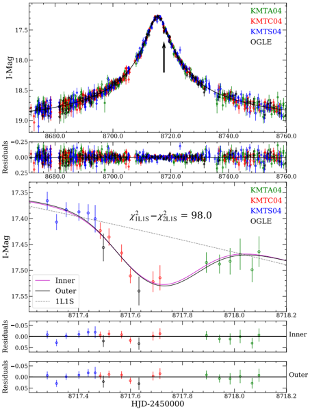
The anomaly of KMT-2019-BLG-1806 is also a dip, as shown in Figure 5. The dip has ∆ t dip ∼ 0 . 6 days and centers on t anom ∼ 8717 . 72 . The dip is defined by the KMTC data and the two contemporaneous OGLE points, which were taken in good seeing ( 1 . ′′ 1 -2 . ′′ 4 ) and low sky background. Hence, the anomaly is secure. Applying the heuristic formalism of Section 4.1, we obtain
<!-- formula-not-decoded -->
In addition, given the Einstein timescale ( t E ∼ 135 days), we expect that π E should be either measured or strongly constrained.
The 2L1S modeling also finds a pair of inner/outer solutions and combined the u 0 > 0 and u 0 < 0 degeneracy
## ZANG ET AL.
Table 4. 2L1S Parameters KMT-2019-BLG-1806
| Parameter | Inner | Inner | Outer | Outer |
|---------------|----------------------|-----------------------|----------------------|-----------------------|
| | u 0 > 0 | u 0 < 0 | u 0 > 0 | u 0 < 0 |
| χ 2 /dof | 3132.5/3132 | 3132.9/3132 | 3132.2/3132 | 3131.8/3132 |
| t 0 ( HJD ′ ) | 8715 . 452 ± 0 . 015 | 8715 . 451 ± 0 . 015 | 8715 . 453 ± 0 . 014 | 8715 . 453 ± 0 . 015 |
| u 0 | 0 . 0260 ± 0 . 0017 | - 0 . 0251 ± 0 . 0020 | 0 . 0257 ± 0 . 0016 | - 0 . 0255 ± 0 . 0015 |
| t E (days) | 132 . 8 ± 8 . 1 | 138 . 5 ± 10 . 8 | 134 . 1 ± 7 . 9 | 135 . 6 ± 7 . 9 |
| ρ (10 - 3 ) | < 1 . 8 | < 1 . 8 | < 1 . 9 | < 1 . 7 |
| α (rad) | 2 . 150 ± 0 . 008 | - 2 . 147 ± 0 . 008 | 2 . 151 ± 0 . 009 | - 2 . 148 ± 0 . 008 |
| s | 0 . 9377 ± 0 . 0069 | 0 . 9383 ± 0 . 0073 | 1 . 0339 ± 0 . 0084 | 1 . 0352 ± 0 . 0085 |
| log q | - 4 . 724 ± 0 . 117 | - 4 . 734 ± 0 . 109 | - 4 . 717 ± 0 . 117 | - 4 . 714 ± 0 . 116 |
| π E , N | - 0 . 055 ± 0 . 150 | - 0 . 066 ± 0 . 161 | - 0 . 060 ± 0 . 156 | - 0 . 019 ± 0 . 160 |
| π E , E | - 0 . 058 ± 0 . 017 | - 0 . 059 ± 0 . 014 | - 0 . 057 ± 0 . 017 | - 0 . 060 ± 0 . 013 |
| I S | 21 . 33 ± 0 . 07 | 21 . 37 ± 0 . 09 | 21 . 34 ± 0 . 07 | 21 . 35 ± 0 . 07 |
there are four solutions in total. See Table 4 for their parameters. The inclusion of π E improves the fits by ∆ χ 2 = 31 , and all four data sets contribute to the improvement, so the parallax signal is reliable. The angle of the minor axis of the parallax ellipse (north through east) is ψ = 82 . 0 ◦ and ψ = 82 . 5 ◦ for the u 0 > 0 and u 0 < 0 solutions, respectively. π E , ‖ = 0 . 06 ± 0 . 01 , and π E , ⊥ is constrained to be σ ( π E , ⊥ ) ∼ 0 . 2 . We obtain s mean = 0 . 985 ± 0 . 008 , α = 123 . 1 ± 0 . 5 , and log q ∼ -4 . 72 , in good agreement with Equation (12). The ratio of the phase-space factors is p inner : p outer = 0 . 80 : 1 .
We find that the inclusion of the lens orbital motion effect only improves the fit by ∆ χ 2 < 1 for 2 degree-of-freedom and is not correlated with π E , so we exclude the lens orbital motion effect. With q ∼ 1 . 9 × 10 -5 , this new planet is the fifth robust q < 2 × 10 -5 microlensing planet.
## 4.2.4. KMT-2017-BLG-1003
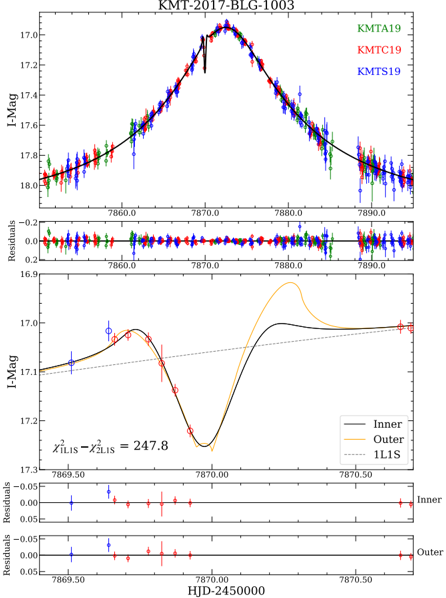
Figure 6 shows the light curve and the best-fit models for KMT-2017-BLG-1003. The KMTC data show a sudden dip and the ridge is confirmed by the KMTC and KMTS data. These data were taken in good seeing ( 1 . ′′ 2 -2 . ′′ 2 ) and low sky background, so the anomaly is of astrophysical origin. Although the end of the dip is not covered, the KMTC point at HJD ′ = 7870 . 66 indicates ∆ t dip < 0 . 85 days, which yields
<!-- formula-not-decoded -->
The numerical analysis yields a pair of inner/outer solutions, and Table 5 lists their parameters. As shown in Figure 2, the 'Outer' solution has caustic crossings, so its ρ is measured at the 4 . 5 σ level. For the 'Inner' solution, a pointsource model is consistent within 2 σ . We note that the geometric mean of s , s mean = 0 . 899 ± 0 . 004 , which is slightly
Figure 6. Light curve and models for KMT-2017-BLG-1003. The symbols are similar to those in Figure 1.
<details>
<summary>Image 6 Details</summary>
### Visual Description
## Light Curve Analysis: KMT-2017-BLG-1003
### Overview
The image presents a light curve analysis of the microlensing event KMT-2017-BLG-1003. It consists of two main panels, each containing a light curve plot and corresponding residuals. The top panel shows the full light curve with data from multiple telescopes, while the bottom panel focuses on a zoomed-in region around the peak of the event. The data is presented as magnitude (I-Mag) versus time (HJD-2450000).
### Components/Axes
* **X-axis (Both Panels):** HJD-2450000 (Heliocentric Julian Date minus 2450000). Scale ranges from approximately 7860 to 7890 in the top panel and 7869.5 to 7870.5 in the bottom panel.
* **Y-axis (Top & Bottom Panels):** I-Mag (Magnitude in the I-band). Scale ranges from approximately 16.9 to 18.1 in the top panel and 16.9 to 17.2 in the bottom panel.
* **Top Panel Data Series:**
* KMTA19 (Red)
* KMTC19 (Green)
* KMTS19 (Blue)
* **Bottom Panel Data Series:**
* Inner (Black)
* Outer (Orange)
* 1LIS (Gray)
* **Residuals Plots (Both Panels):** Display the difference between the observed data and the model fit. Y-axis ranges from -0.2 to 0.2 in the top panel and -0.05 to 0.05 in the bottom panel.
* **Equation:** χ²<sub>1LIS</sub> - χ²<sub>2LIS</sub> = 247.8 (located in the bottom panel)
* **Legend:** Located in the top-right corner for the top panel data series and bottom-right corner for the bottom panel data series.
### Detailed Analysis or Content Details
**Top Panel:**
* **KMTA19 (Red):** The data points show a general upward trend from approximately 7860 to a peak around 7870, followed by a downward trend to 7890. Values range from approximately 17.8 at 7860 to 17.2 at 7870, then back to 18.0 at 7890. Significant scatter is present.
* **KMTC19 (Green):** Similar trend to KMTA19, but with more scatter. Values range from approximately 17.9 at 7860 to 17.3 at 7870, then back to 18.1 at 7890.
* **KMTS19 (Blue):** Also follows the same trend, with values ranging from approximately 18.0 at 7860 to 17.4 at 7870, then back to 18.2 at 7890.
* **Residuals (Top Panel):** The residuals are generally centered around zero, indicating a reasonable fit. Some scatter is visible, particularly around the peak of the light curve.
**Bottom Panel:**
* **Inner (Black):** A smooth curve representing the inner microlensing solution. It peaks sharply around HJD-2450000 = 7870.0, reaching a minimum magnitude of approximately 17.0.
* **Outer (Orange):** A broader, less pronounced curve representing the outer microlensing solution. It peaks around HJD-2450000 = 7870.0, reaching a minimum magnitude of approximately 17.1.
* **1LIS (Gray):** A line representing the 1LIS model. It is relatively flat and close to the Outer curve.
* **Residuals (Bottom Panel):** The residuals for both the Inner and Outer solutions are small and generally within the error bars.
### Key Observations
* The light curve exhibits a clear microlensing event with a distinct peak.
* The data from the three telescopes (KMTA19, KMTC19, KMTS19) are consistent with each other, although with varying degrees of scatter.
* The bottom panel shows two possible microlensing solutions: an "Inner" solution and an "Outer" solution. The Inner solution provides a better fit to the data, as indicated by the χ² value.
* The χ² difference of 247.8 suggests a statistically significant preference for the 1LIS model over the 2LIS model.
* The residuals are generally small, indicating that the models provide a good fit to the data.
### Interpretation
The data demonstrates a microlensing event caused by the gravitational lensing of a background star by a foreground object. The light curve shows the characteristic brightening of the background star as the lens passes close to its line of sight. The two solutions (Inner and Outer) represent different possible configurations of the lens and source stars. The significantly lower χ² value for the 1LIS model suggests that the "Inner" solution is the more likely scenario. The residuals analysis confirms the goodness of fit of the models to the observed data. The event is well-characterized by the data from the three telescopes, providing a robust measurement of the microlensing parameters. The event is identified as KMT-2017-BLG-1003. The data suggests a relatively close alignment between the lens and source stars, resulting in a significant brightening of the background star. The analysis provides valuable insights into the distribution of stars and compact objects in the Galactic bulge.
</details>
different from s -by 1 σ . This indicates that the prediction of Ryu et al. (2022) might be imperfect for minor-image anomalies with finite-source effects or incomplete coverage. The ratio of the phase-space factors is p inner : p outer = 0 . 80 : 1 .
Table 5. 2L1S Parameters for KMT-2017-BLG-1003
| Parameter | Inner | Outer |
|---------------|----------------------|----------------------|
| χ 2 /dof | 2433.2/2433 | 2433.0/2433 |
| t 0 ( HJD ′ ) | 7872 . 484 ± 0 . 020 | 7872 . 482 ± 0 . 020 |
| u 0 | 0 . 179 ± 0 . 005 | 0 . 179 ± 0 . 005 |
| t E (days) | 25 . 65 ± 0 . 57 | 25 . 66 ± 0 . 59 |
| ρ (10 - 3 ) | < 6 . 7 | 5 . 22 ± 1 . 16 |
| α (rad) | 1 . 073 ± 0 . 006 | 1 . 072 ± 0 . 006 |
| s | 0 . 8889 ± 0 . 0043 | 0 . 9096 ± 0 . 0045 |
| log q | - 4 . 260 ± 0 . 152 | - 4 . 373 ± 0 . 144 |
| I S , OGLE | 19 . 30 ± 0 . 04 | 19 . 30 ± 0 . 04 |
With high-order effects, the χ 2 improvement is 1.7. Although this event is shorter than the first two events, π E is better constrained due to the about one magnitude brighter data, with π E , ‖ = -0 . 11 ± 0 . 15 . This is another Neptune/Sun mass-ratio planet.
## 4.2.5. KMT-2019-BLG-1367
Figure 7. Light curve and models for KMT-2019-BLG-1367. The symbols are similar to those in Figure 1.
<details>
<summary>Image 7 Details</summary>
### Visual Description
## Light Curve Analysis: KMT-2019-BLG-1367
### Overview
The image presents a light curve analysis of the microlensing event KMT-2019-BLG-1367, displaying brightness (I-Mag) over time (HJD-2450000). The data is presented in two main panels, with residual plots below each. The top panel shows data from multiple telescopes (OGLE, KMTA33, KMTC33, KMTS33) and a fitted model. The bottom panel focuses on a zoomed-in view of the peak with a different model fit.
### Components/Axes
* **X-axis (both panels):** HJD-2450000 (Heliocentric Julian Date minus 2450000). Ranges from approximately 8650.0 to 8680.0 in the top panel and 8666.0 to 8667.0 in the bottom panel.
* **Y-axis (top panel):** I-Mag (Instrumental Magnitude). Ranges from approximately 18.5 to 20.5.
* **Y-axis (bottom panel):** I-Mag (Instrumental Magnitude). Ranges from approximately 18.4 to 18.8.
* **Y-axis (Residuals panels):** Residuals (likely magnitude difference between observed and modeled data). Ranges from approximately -0.5 to 0.5 (top residuals) and -0.15 to 0.15 (bottom residuals).
* **Legend (top-right of top panel):**
* OGLE (Green)
* KMTA33 (Blue)
* KMTC33 (Red)
* KMTS33 (Cyan)
* **Legend (bottom-right of bottom panel):**
* Inner (Black)
* Outer (Yellow)
* 1L1S (Gray)
* **Text:** "KMT-2019-BLG-1367" (top-left)
* **Text:** "χ<sup>2</sup><sub>LIS</sub> - χ<sup>2</sup><sub>1L1S</sub> = 82.3" (bottom-left of bottom panel)
### Detailed Analysis or Content Details
**Top Panel:**
* **OGLE (Green):** Data points are scattered, with a peak magnitude around 18.6 at HJD ~ 8668.0. Error bars are visible, ranging from approximately 0.02 to 0.05.
* **KMTA33 (Blue):** Similar trend to OGLE, peaking around 18.6 at HJD ~ 8668.0. Error bars are similar in size to OGLE.
* **KMTC33 (Red):** Also peaks around 18.6 at HJD ~ 8668.0. Error bars are slightly larger, ranging from approximately 0.03 to 0.07.
* **KMTS33 (Cyan):** Peaks around 18.6 at HJD ~ 8668.0. Error bars are similar to KMTA33.
* **Black Curve:** A smooth curve fitting the data, representing the model. The curve shows a clear peak around HJD 8668.0, with a gradual increase and decrease in brightness.
**Top Residuals Panel:**
* Residuals for all telescopes (colored points) are mostly within the -0.5 to 0.5 range, indicating a reasonable fit. There are some deviations, particularly around the peak.
**Bottom Panel:**
* **Inner (Black):** A smooth curve representing the inner source contribution. It shows a dip in brightness around HJD 8666.6.
* **Outer (Yellow):** A smooth curve representing the outer source contribution. It shows a peak in brightness around HJD 8666.8.
* **1L1S (Gray):** A smooth curve representing the 1L1S model.
* **Red Data Points:** Data points with error bars, peaking around 18.6 at HJD ~ 8666.8. Error bars range from approximately 0.02 to 0.05.
**Bottom Residuals Panel:**
* Residuals for the Inner source (black points) are mostly within the -0.15 to 0.15 range.
* Residuals for the Outer source (red points) are also mostly within the -0.15 to 0.15 range.
### Key Observations
* The light curve exhibits a clear microlensing event, with a peak brightness around I-Mag 18.6.
* The different telescopes (OGLE, KMTA33, KMTC33, KMTS33) provide consistent data, as evidenced by the overlapping data points in the top panel.
* The residuals suggest a good fit between the model and the observed data, although some deviations are present.
* The bottom panel provides a more detailed view of the peak, showing the contributions of the inner and outer sources.
* The χ<sup>2</sup> value indicates the quality of the fit. A value of 82.3 suggests a reasonably good fit, but further statistical analysis would be needed to determine its significance.
### Interpretation
This data represents a microlensing event, where the gravity of a foreground star bends and magnifies the light from a background star. The light curve shows the characteristic brightening and dimming as the alignment between the observer, lens star, and source star changes. The different telescopes provide independent measurements, increasing the confidence in the results. The model fitting (black curve in the top panel, and inner/outer curves in the bottom panel) allows astronomers to estimate the properties of the lens star, such as its mass and distance. The residuals help assess the quality of the fit and identify any systematic errors in the data. The χ<sup>2</sup> value provides a quantitative measure of the goodness of fit. The zoomed-in view in the bottom panel allows for a more precise analysis of the peak, which is crucial for determining the properties of the lens system. The 1L1S model likely represents a single lens and single source model. The difference in χ<sup>2</sup> values suggests that the 1L1S model is a better fit than another model (LIS). This analysis is important for studying the distribution of stars and planets in the galaxy.
</details>
Table 6. 2L1S Parameters for KMT-2019-BLG-1367
| Parameter | Inner | Outer |
|---------------|----------------------|----------------------|
| χ 2 /dof | 1404.0/1404 | 1404.2/1404 |
| t 0 ( HJD ′ ) | 8667 . 883 ± 0 . 051 | 8667 . 884 ± 0 . 048 |
| u 0 | 0 . 083 ± 0 . 009 | 0 . 082 ± 0 . 009 |
| t E (days) | 39 . 3 ± 3 . 8 | 39 . 8 ± 4 . 0 |
| ρ (10 - 3 ) | < 5 . 3 | < 5 . 6 |
| α (rad) | 1 . 208 ± 0 . 016 | 1 . 207 ± 0 . 016 |
| s | 0 . 9389 ± 0 . 0066 | 0 . 9763 ± 0 . 0070 |
| log q | - 4 . 303 ± 0 . 118 | - 4 . 298 ± 0 . 103 |
| I S , OGLE | 21 . 46 ± 0 . 13 | 21 . 48 ± 0 . 13 |
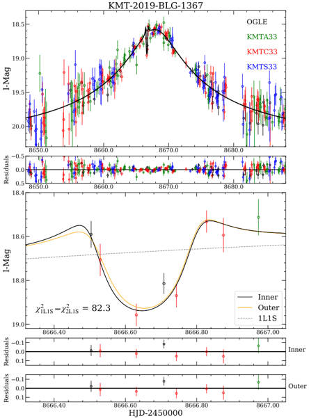
Figure 7 shows a dip 1.2 days before the peak of an otherwise normal PSPL event, with a duration of ∆ t dip ∼ 0 . 35 days. The dip-type anomaly is covered by the KMTC data and one contemporaneous OGLE point, and these data were taken in good seeing ( < 2 . ′′ 0 ) and low sky background. Therefore, the anomaly is secure. Applying the heuristic formalism of Section 4.1, we obtain
<!-- formula-not-decoded -->
The 2L1S modeling also yields a pair of inner/outer solutions, with ∆ χ 2 = 0 . 2 . The resulting solutions are given in Table 6 and Figure 2. A point-source model is consistent within 1 σ and the 3 σ upper limit is ρ < 0 . 0056 , so we expect that the Ryu et al. (2022) formula is applicable. We obtain s mean = 0 . 957 ± 0 . 007 , in good agreement with s -. The ratio of the phase-space factors is p inner : p outer = 0 . 82 : 1 . We find that the inclusion of higher-order effects only improves the fitting by ∆ χ 2 < 1 and the 1 σ uncertainty of parallax is > 0 . 9 at all directions, so the constraint on π E is not useful for the Bayesian analysis. This is another planet with a Neptune/Sun mass ratio.
## 4.3. 'Bump' Anomalies
For bump-type planetary signals, we also check whether the observed data can be fitted by a single-lens binary-source (1L2S) model (Gaudi 1998) because it can also produce such anomalies (e.g., Hwang et al. 2013; Jung et al. 2017; Rota et al. 2021). For a 1L2S model, its magnification, A λ , is the superposition of magnifications for two single-lens singlesource (1L1S) models,
<!-- formula-not-decoded -->
where f i ,λ is the source flux at wavelength λ , and i = 1 and i = 2 correspond to the primary and the secondary sources, respectively.
## 4.3.1. OGLE-2017-BLG-1806
Figure 8. Light curve and models for OGLE-2017-BLG-1806. The symbols are similar to those in Figure 1. Different with the previous four events, the anomaly is bump-type, so the best-fit 1L2S model is provided.
<details>
<summary>Image 8 Details</summary>
### Visual Description
\n
## Light Curve Analysis: OGLE-2017-BLG-1806
### Overview
The image presents a light curve analysis of the microlensing event OGLE-2017-BLG-1806. It consists of three subplots, each displaying the I-band magnitude (I-Mag) over time (HJD-2450000). The top subplot shows the overall light curve with multiple observational datasets. The middle subplot focuses on the peak of the microlensing event, with additional model fits. The bottom subplot displays the residuals for each dataset.
### Components/Axes
* **X-axis (all subplots):** HJD-2450000 (Heliocentric Julian Date - 2450000). Scale ranges from approximately 8000.0 to 8060.0.
* **Y-axis (top & middle subplots):** I-Mag (I-band Magnitude). Scale ranges from approximately 17.5 to 19.5 (top) and 19.2 to 19.8 (middle).
* **Y-axis (bottom subplots):** Residuals. Scale ranges from approximately -0.25 to 0.25.
* **Legend (middle subplot, bottom-right):**
* OGLE (Black)
* KMTA19 (Red)
* KMTC19 (Blue)
* KMTS19 (Green)
* Close A (Dark Cyan)
* Close B (Dark Red)
* Wide (Dark Green)
* 1L2S (Dark Blue)
* 1L1S (Dark Magenta)
* **Title (top subplot):** OGLE-2017-BLG-1806
* **Text (middle subplot, bottom-center):** χ<sup>2</sup><sub>LIS</sub> - χ<sup>2</sup><sub>ILIS</sub> = 126.3
### Detailed Analysis or Content Details
**Top Subplot:**
* The light curve shows a clear microlensing event, with a peak around HJD-2450000 = 8040.0.
* OGLE (Black): Data points are sparse, showing a general upward trend before the peak and a downward trend after. Magnitude values range from approximately 18.2 to 19.2.
* KMTA19 (Red): Data points are more densely populated around the peak. Magnitude values range from approximately 17.8 to 19.5. The curve shows a sharp increase to the peak and a slower decrease.
* KMTC19 (Blue): Similar to KMTA19, with a peak magnitude around 18.0 and a range of 18.0 to 19.3.
* KMTS19 (Green): Data points are concentrated around the peak, with magnitude values ranging from approximately 18.1 to 19.4.
**Middle Subplot:**
* This subplot focuses on the peak of the microlensing event.
* The best-fit model (black line) closely follows the KMTA19 (red), KMTC19 (blue), and KMTS19 (green) data points around the peak.
* Close A (Dark Cyan): A relatively flat line around I-Mag = 19.7.
* Close B (Dark Red): A relatively flat line around I-Mag = 19.7.
* Wide (Dark Green): A relatively flat line around I-Mag = 19.7.
* 1L2S (Dark Blue): A relatively flat line around I-Mag = 19.7.
* 1L1S (Dark Magenta): A relatively flat line around I-Mag = 19.7.
* The peak magnitude is approximately 17.8 (from KMTA19, KMTC19, and KMTS19).
**Bottom Subplots:**
* These subplots show the residuals (difference between observed data and model) for each dataset.
* OGLE (top): Residuals are scattered around zero, with some positive and negative deviations.
* KMTA19 (middle): Residuals are generally small, indicating a good fit.
* KMTC19 (bottom): Residuals are generally small, indicating a good fit.
* KMTS19 (bottom): Residuals are generally small, indicating a good fit.
* Close A (top): Residuals are scattered around zero.
* Close B (middle): Residuals are scattered around zero.
* Wide (bottom): Residuals are scattered around zero.
* 1L2S (bottom): Residuals are scattered around zero.
### Key Observations
* The microlensing event shows a well-defined peak, indicating a clear alignment between the source star, lens star, and observer.
* The KMTA19, KMTC19, and KMTS19 datasets provide the most detailed coverage of the peak, allowing for a precise determination of the event parameters.
* The residuals are generally small, suggesting that the model provides a good fit to the observed data.
* The χ<sup>2</sup><sub>LIS</sub> - χ<sup>2</sup><sub>ILIS</sub> value of 126.3 indicates the quality of the fit.
### Interpretation
The data demonstrates a microlensing event caused by a foreground star (the lens) passing in front of a background star (the source). The brightening of the source star's light is due to the gravitational focusing effect of the lens. The shape of the light curve provides information about the mass of the lens, its distance from the source, and its relative motion. The multiple datasets (OGLE, KMTA19, KMTC19, KMTS19) provide independent measurements of the light curve, allowing for a robust analysis. The residuals indicate the accuracy of the model used to fit the data. The different model fits (Close A, Close B, Wide, 1L2S, 1L1S) likely represent different possible configurations of the lens system, and the best-fit model is chosen based on the lowest residuals and the χ<sup>2</sup> value. The value of χ<sup>2</sup><sub>LIS</sub> - χ<sup>2</sup><sub>ILIS</sub> = 126.3 is a statistical measure of the goodness of fit, with lower values indicating a better fit. The data suggests a relatively simple microlensing event, with no evidence of complex features such as planetary companions or binary lenses.
</details>
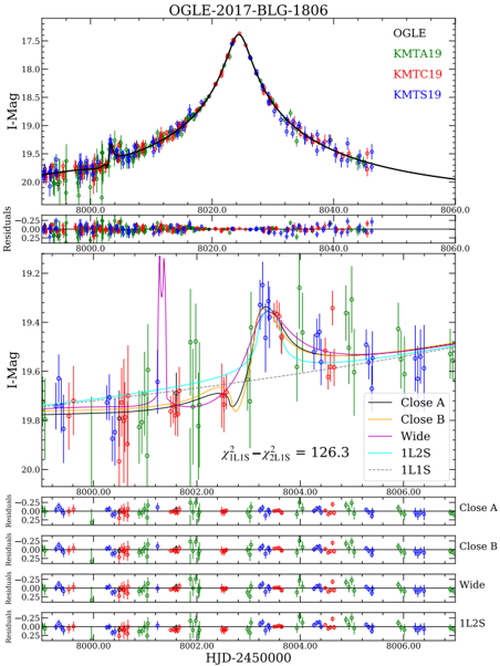
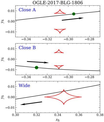
As shown in Figure 8, the light curve of OGLE-2017-BLG1806 exhibits a bump centered on t anom ∼ 8003 . 5 , defined by the KMTC and KMTS data. Except for two KMTS points, all the KMTC and KMTS data during 8003 < HJD ′ < 8005 were taken in good seeing ( < 2 . ′′ 2 ) and low sky background. In addition, most of the data before the bump ( 8000 < HJD ′ < 8003 ) are fainter than the 1L1S model. Hence, the signal is secure. Because both the major-image and the two minor-image planetary caustics can produce a bump-type anomaly (e.g., Wang et al. 2022), we obtain
<!-- formula-not-decoded -->
The grid search returns three local minima, and their caustic structures are given in Figure 9. As expected, the three solutions respectively correspond to sources crossing a majorimage (quadrilateral) planetary caustic and two minor-image (triangular) planetary caustics. We label the three solutions as 'Close A', 'Close B', and 'Wide', respectively, and their parameters are presented in Table 7.
y
y
y
Figure 9. Geometries of OGLE-2017-BLG-1806. The symbols are similar to those in Figure 2. For the two 'Close' solutions, ρ is constrained at the > 3 σ level, so the radius of the two green dots represent the source radius. For the 'Wide' solution, ρ only has weak constraints with < 3 σ , so its source radius is not shown.
<details>
<summary>Image 9 Details</summary>
### Visual Description
## Chart: Microlensing Event OGLE-2017-BLG-1806
### Overview
The image presents three separate charts displaying data related to a microlensing event designated OGLE-2017-BLG-1806. Each chart represents a different observational setup or filter: "Close A", "Close B", and "Wide". The charts plot the y-coordinate (Ys) against the x-coordinate (Xs), likely representing the relative positions of source, lens, and observer during the event. Each chart includes a black line representing a model fit to the data, and red symbols representing observed data points. Green dots with arrows indicate the direction of time progression.
### Components/Axes
* **Title:** OGLE-2017-BLG-1806 (top-center)
* **X-axis Label:** Xs (bottom-center of each chart)
* **Y-axis Label:** Ys (left-side of each chart)
* **Charts:** Three sub-charts labeled "Close A", "Close B", and "Wide" (top-left of each chart).
* **Data Points:** Red symbols (various shapes) representing observed data.
* **Model Fit:** Black solid lines representing the theoretical model.
* **Time Progression:** Green dots with arrows indicating the direction of time.
### Detailed Analysis or Content Details
**Close A Chart:**
* **X-axis Range:** Approximately -0.34 to -0.28
* **Y-axis Range:** Approximately -0.01 to 0.01
* **Model Fit:** The black line slopes upward with a slight positive gradient.
* **Data Points:**
* First data point (top-right): Xs ≈ -0.31, Ys ≈ 0.008
* Second data point (bottom-right): Xs ≈ -0.31, Ys ≈ -0.005
* Third data point (bottom-left): Xs ≈ -0.33, Ys ≈ -0.003
* **Time Progression:** Arrow points from left to right.
**Close B Chart:**
* **X-axis Range:** Approximately -0.34 to -0.28
* **Y-axis Range:** Approximately -0.01 to 0.01
* **Model Fit:** The black line is initially relatively flat, then curves upward.
* **Data Points:**
* First data point (top-right): Xs ≈ -0.31, Ys ≈ 0.008
* Second data point (bottom-right): Xs ≈ -0.31, Ys ≈ -0.005
* Third data point (bottom-left): Xs ≈ -0.33, Ys ≈ -0.003
* **Time Progression:** Arrow points from left to right.
**Wide Chart:**
* **X-axis Range:** Approximately 0.30 to 0.38
* **Y-axis Range:** Approximately -0.01 to 0.01
* **Model Fit:** The black line slopes upward with a positive gradient.
* **Data Points:** Multiple red symbols are present, forming a more complex pattern.
* First data point (top-right): Xs ≈ 0.34, Ys ≈ 0.006
* Second data point (center-right): Xs ≈ 0.35, Ys ≈ 0.002
* Third data point (bottom-right): Xs ≈ 0.36, Ys ≈ -0.002
* Fourth data point (bottom-left): Xs ≈ 0.32, Ys ≈ -0.004
* Fifth data point (center-left): Xs ≈ 0.31, Ys ≈ 0.001
* **Time Progression:** Arrow points from left to right.
### Key Observations
* All three charts show a general upward trend in the model fit lines.
* The "Wide" chart exhibits a more complex data pattern with more data points than the "Close A" and "Close B" charts.
* The green dots with arrows consistently indicate a progression of time from left to right in all charts.
* The data points in all charts appear to generally follow the trend of the model fit lines, but with some deviations.
### Interpretation
These charts represent the light curve of a microlensing event. Microlensing occurs when a massive object (the lens) passes between a distant source star and the observer (Earth). The gravity of the lens bends the light from the source star, causing it to appear brighter and potentially distorted.
The three charts likely represent observations taken with different filters or at different times during the event. The "Close A" and "Close B" charts might represent observations taken closer to the peak of the event, while the "Wide" chart could represent observations taken further away from the peak.
The model fit lines represent the theoretical prediction of how the light curve should look based on the properties of the lens and source star. The data points represent the actual observed brightness of the source star. The differences between the data points and the model fit lines could be due to various factors, such as noise in the data, the presence of other objects in the field of view, or inaccuracies in the model.
The upward trend in the model fit lines suggests that the lens is moving across the line of sight to the source star, causing the brightness of the source star to increase. The more complex pattern in the "Wide" chart could indicate that the event is more complex than a simple single-lens microlensing event, potentially involving multiple lenses or a binary lens system. The green arrows indicate the direction of time, allowing us to track the evolution of the microlensing event.
</details>
The 'Close A' solution provides the best fit to the observed data, and the 'Close B' and 'Wide' solutions are disfavored by ∆ χ 2 = 14 . 1 and 8.3, respectively. We find that the inclusion of the parallax effect improves the fit by ∆ χ 2 = 7.8, 20.4, and 11.1 for the 'Close A', 'Close B', and 'Wide' solutions, respectively, and during the anomaly region ( 7998 < HJD ′ < 8008 ), ∆ χ 2 = 2.2, 22.3, and 6.8. With the anomaly removed, fitting the data by a 1L1S model yields a similar constraint on π E , ‖ and a weaker constraint on π E , ⊥ , with σ ( π E , ⊥ ) ∼ 0 . 5 . Thus, the long planetary signal plays an important role in improving the constraint on π E , ⊥ and reduces the χ 2 differences between the three solutions.
The ratio of the phase-space factors is p CloseA : p CloseB : p Wide = 1 : 0 . 95 : 0 . 61 . For the 'Close A', and 'Close B' solutions, the bump was produced by a caustic crossing, so ρ is constrained at the > 3 σ level. For the 'Wide' solution, the bump was a result of a cusp approach. Although the 'Wide' solution has caustic crossing features, due to the lack of data during the crossing, a point-source model is consistent within 1 σ .
The 1L2S model is disfavored by ∆ χ 2 = 30 . 7 compared to the 'Close A' solution, and the 1L2S parameters are shown in Table 8. Although the 1L2S model fits the bump well, it provides a worse fit to the observed data before the bump, during which most of the data from the three KMTNet sites
Table 7. 2L1S Parameters for OGLE-2017-BLG-1806
| Parameter | Close A | Close A | Close B | Close B | Wide | Wide |
|---------------|-------------------------|-------------------------|-------------------------|-------------------------|----------------------|-----------------------|
| χ 2 /dof | u 0 > 0 1650.9/1651 | u 0 < 0 1650.7/1651 | u 0 > 0 1664.8/1651 | u 0 < 0 1665.5/1651 | u 0 > 0 1659.1/1651 | u 0 < 0 1659.0/1651 |
| t 0 ( HJD ′ ) | 8024 . 392 ± 0 . 020 | 8024 . 393 ± 0 . 019 | 8024 . 388 ± 0 . 020 | 8024 . 388 ± 0 . 020 | 8024 . 388 ± 0 . 020 | 8024 . 379 ± 0 . 020 |
| u 0 | 0 . 0249 ± 0 . 0016 | - 0 . 0260 ± 0 . 0016 | 0 . 0256 ± 0 . 0020 | - 0 . 0253 ± 0 . 0019 | 0 . 0269 ± 0 . 0018 | - 0 . 0257 ± 0 . 0017 |
| t E (days) | 69 . 4 ± 4 . 0 | 66 . 8 ± 3 . 9 | 69 . 4 ± 4 . 8 | 69 . 6 ± 4 . 6 | 64 . 5 ± 3 . 9 | 67 . 0 ± 3 . 9 |
| ρ (10 - 3 ) | 1 . 74 +0 . 78 - 0 . 44 | 1 . 83 +0 . 80 - 0 . 50 | 1 . 50 +0 . 62 - 0 . 47 | 1 . 65 +0 . 67 - 0 . 50 | < 2 . 8 | < 2 . 4 |
| α (rad) | 0 . 001 ± 0 . 034 | - 0 . 002 ± 0 . 037 | 0 . 267 ± 0 . 066 | - 0 . 263 ± 0 . 068 | 3 . 121 ± 0 . 034 | - 3 . 121 ± 0 . 036 |
| s | 0 . 8609 ± 0 . 0069 | 0 . 8566 ± 0 . 0075 | 0 . 8592 ± 0 . 0085 | 0 . 8601 ± 0 . 0080 | 1 . 1900 ± 0 . 0117 | 1 . 1806 ± 0 . 0108 |
| log q | - 4 . 392 ± 0 . 180 | - 4 . 352 ± 0 . 171 | - 4 . 766 ± 0 . 220 | - 4 . 768 ± 0 . 209 | - 4 . 317 ± 0 . 126 | - 4 . 441 ± 0 . 168 |
| π E , N | - 0 . 278 ± 0 . 148 | 0 . 292 ± 0 . 170 | 0 . 774 ± 0 . 315 | - 0 . 756 ± 0 . 326 | - 0 . 535 ± 0 . 175 | 0 . 504 ± 0 . 170 |
| π E , E | 0 . 105 ± 0 . 056 | 0 . 144 ± 0 . 058 | 0 . 157 ± 0 . 070 | 0 . 124 ± 0 . 059 | 0 . 120 ± 0 . 065 | 0 . 133 ± 0 . 056 |
| I S , KMTC | 21 . 12 ± 0 . 07 | 21 . 07 ± 0 . 07 | 21 . 10 ± 0 . 08 | 21 . 10 ± 0 . 08 | 21 . 03 ± 0 . 07 | 21 . 08 ± 0 . 07 |
Table 8. 1L2S Parameters for OGLE-2017-BLG-1806 and KMT-2016-BLG-1105
| Parameters | OGLE-2017-BLG-1806 | OGLE-2017-BLG-1806 | KMT-2016-BLG-1105 |
|-------------------|-------------------------|-------------------------|----------------------|
| χ 2 /dof | u 0 > 0 1682 . 0 / 1651 | u 0 < 0 1681 . 4 / 1651 | 2298 . 7 / 2288 |
| t 0 , 1 ( HJD ′ ) | 8024 . 383 ± 0 . 020 | 8024 . 381 ± 0 . 020 | 7555 . 972 ± 0 . 094 |
| t 0 , 2 ( HJD ′ ) | 8003 . 876 ± 0 . 274 | 8003 . 913 ± 0 . 253 | 7547 . 890 ± 0 . 021 |
| u 0 , 1 | 0 . 0288 ± 0 . 0023 | - 0 . 0282 ± 0 . 0019 | 0 . 143 ± 0 . 022 |
| u 0 , 2 | 0 . 003 ± 0 . 025 | - 0 . 004 ± 0 . 023 | 0 . 0001 ± 0 . 0007 |
| t E (days) | 61 . 2 ± 4 . 3 | 62 . 2 ± 3 . 5 | 44 . 9 ± 5 . 8 |
| ρ 2 ( 10 - 3 ) | < 7 . 3 | < 7 . 0 | < 3 . 3 |
| q f,I (10 - 3 ) | 2 . 76 ± 0 . 76 | 2 . 63 ± 0 . 74 | 1 . 98 ± 0 . 48 |
| π E , N | 0 . 041 ± 0 . 388 | 0 . 059 ± 0 . 355 | ... |
| π E , E | 0 . 111 ± 0 . 072 | 0 . 117 ± 0 . 063 | ... |
| I S , KMTC | 20 . 96 ± 0 . 09 | 20 . 98 ± 0 . 07 | 21 . 31 ± 0 . 18 |
are fainter than the 1L2S model. Hence, the 1L2S model is rejected. We find that the lens orbital motion effect is not detectable ( ∆ χ 2 < 0 . 5 ), so we adopt the parameters with the microlensing parallax effect as our final results.
## 4.3.2. KMT-2016-BLG-1105
The anomaly in Figure 10 is a short-lived bump centered on t anom ∼ 7547 . 85 , which is defined by four KMTC data points and supported by one OGLE data point. These data were taken in good seeing ( < 2 . ′′ 0 ) and low sky background, so the anomaly is secure. Similar to OGLE-2017-BLG-1806, we expect both the major-image and the minor-image plane- tary caustics can produce the bump and obtain
<!-- formula-not-decoded -->
The 2L1S modeling yields five solutions, including one with the minor-image planetary caustics and four with the major-image planetary caustics. We label them as 'Close', 'Wide A', 'Wide B', 'Wide C' and 'Wide D', respectively, and their parameters are given in Table 9. Figure 11 displays the caustic structures and source trajectories. The 'Wide A', 'Wide B' and 'Close' solutions exhibit caustic crossings, but only for the 'Wide B' and 'Close' solutions ρ are constrained at the > 3 σ level. For the 'Wide A', 'Wide C' and 'Wide D' solutions, a point-source model is consistent
Table 9. 2L1S Parameters for KMT-2016-BLG-1105
| Parameters | Wide A | Wide B | Wide C | Wide D | Close |
|----------------|----------------------|----------------------|----------------------|----------------------|----------------------|
| χ 2 /dof | 2286 . 7 / 2288 | 2289 . 0 / 2288 | 2291 . 1 / 2288 | 2289 . 4 / 2288 | 2290 . 2 / 2288 |
| t 0 ( HJD ′ ) | 7555 . 834 ± 0 . 096 | 7555 . 789 ± 0 . 102 | 7555 . 772 ± 0 . 093 | 7555 . 781 ± 0 . 099 | 7555 . 896 ± 0 . 093 |
| u 0 | 0 . 171 ± 0 . 012 | 0 . 153 ± 0 . 013 | 0 . 154 ± 0 . 014 | 0 . 154 ± 0 . 014 | 0 . 148 ± 0 . 008 |
| t E (days) | 38 . 8 ± 2 . 0 | 42 . 4 ± 2 . 9 | 42 . 5 ± 3 . 1 | 42 . 4 ± 3 . 1 | 43 . 3 ± 1 . 8 |
| ρ 1 ( 10 - 3 ) | < 2 . 4 | 2 . 92 ± 0 . 82 | < 4 . 6 | < 5 . 5 | 0 . 75 ± 0 . 14 |
| α (rad) | 3 . 836 ± 0 . 014 | 3 . 830 ± 0 . 016 | 3 . 832 ± 0 . 014 | 3 . 831 ± 0 . 014 | 0 . 691 ± 0 . 021 |
| s | 1 . 143 ± 0 . 009 | 1 . 136 ± 0 . 011 | 1 . 155 ± 0 . 012 | 1 . 106 ± 0 . 013 | 0 . 888 ± 0 . 007 |
| log q | - 5 . 194 ± 0 . 248 | - 4 . 423 ± 0 . 197 | - 4 . 069 ± 0 . 182 | - 4 . 184 ± 0 . 206 | - 5 . 027 ± 0 . 080 |
| I S , KMTC | 21 . 09 ± 0 . 08 | 21 . 20 ± 0 . 05 | 21 . 22 ± 0 . 11 | 21 . 22 ± 0 . 11 | 21 . 27 ± 0 . 06 |
Figure 10. Light curve and models for KMT-2016-BLG-1105. The symbols are similar to those in Figure 1. Because a 1L2S model can produce a short-lived bump, the best-fit 1L2S model is also shown.
<details>
<summary>Image 10 Details</summary>
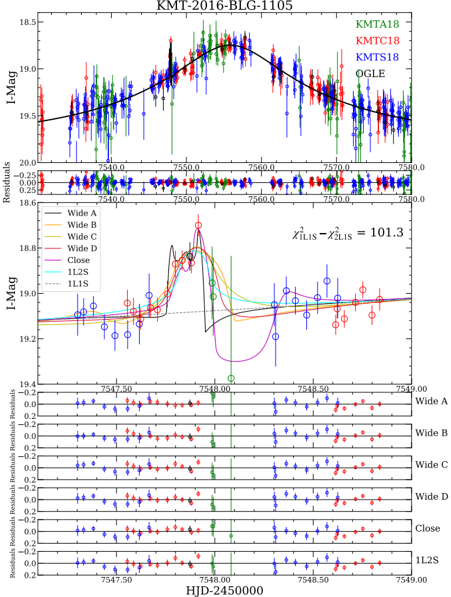
### Visual Description
## Light Curve Analysis: KMT-2016-BLG-1105
### Overview
The image presents a light curve analysis of the microlensing event KMT-2016-BLG-1105. It consists of two main panels, each displaying a light curve (I-Mag vs. HJD-2450000) and corresponding residuals. The top panel shows the overall light curve with multiple datasets, while the bottom panel focuses on the peak of the event with a more detailed view of different datasets.
### Components/Axes
* **X-axis (both panels):** HJD-2450000 (Heliocentric Julian Date minus 2450000). Scale ranges from approximately 7547.0 to 7580.0 in the top panel and 7547.50 to 7549.00 in the bottom panel.
* **Y-axis (both panels):** I-Mag (Magnitude in the I-band). Scale ranges from approximately 18.5 to 20.0 in the top panel and 18.8 to 19.4 in the bottom panel.
* **Residuals (below each light curve):** Residuals are plotted against HJD-2450000. Y-axis scale ranges from approximately -0.25 to 0.25.
* **Legend (top-left of top panel):**
* KMTA18 (Black)
* KMTC18 (Green)
* KMTS18 (Blue)
* OGLE (Red)
* **Legend (left of bottom panel):**
* Wide A (Red)
* Wide B (Orange)
* Wide D (Yellow)
* Close (Magenta)
* 1L2S (Cyan)
* 1LIS (Black)
* **Equation (top-right of bottom panel):** χ²LIS - χ²2LS = 101.3
### Detailed Analysis or Content Details
**Top Panel:**
* **KMTA18 (Black):** The data points are scattered, with a general trend of decreasing magnitude from approximately 7547.0 to 7550.0, reaching a minimum around 19.2, then increasing again to around 19.8 by 7580.0. Error bars are visible, ranging from approximately 0.05 to 0.2.
* **KMTC18 (Green):** Similar trend to KMTA18, but with fewer data points. Magnitude decreases from approximately 19.5 to 19.2 between 7547.0 and 7550.0, then increases to around 19.7 by 7580.0. Error bars are similar in size to KMTA18.
* **KMTS18 (Blue):** Shows a similar trend, with a decrease in magnitude to around 19.2 at 7550.0, followed by an increase to approximately 19.8 by 7580.0. Error bars are comparable to the other datasets.
* **OGLE (Red):** Displays a similar pattern, with a decrease to around 19.2 at 7550.0 and an increase to approximately 19.7 by 7580.0. Error bars are generally smaller than those of the KMTA datasets.
**Bottom Panel:**
* **Wide A (Red):** Relatively constant magnitude around 19.1-19.2, with small fluctuations. Error bars are approximately 0.05.
* **Wide B (Orange):** Similar to Wide A, with a constant magnitude around 19.1-19.2. Error bars are approximately 0.05.
* **Wide D (Yellow):** Constant magnitude around 19.1-19.2. Error bars are approximately 0.05.
* **Close (Magenta):** Shows a significant increase in brightness around HJD-2450000 = 7548.2, peaking at approximately 18.9, then decreasing rapidly. Error bars are initially small (around 0.05) but increase as the brightness peaks.
* **1L2S (Cyan):** Similar to Close, with a peak around 18.9 at 7548.2, followed by a decrease. Error bars are comparable to Close.
* **1LIS (Black):** Shows a smooth curve, with a slight increase in magnitude around 7548.2, but not as pronounced as the other datasets. Error bars are approximately 0.05.
**Residuals:**
* The residuals for all datasets appear randomly scattered around zero, indicating a good fit of the model to the data.
### Key Observations
* The microlensing event shows a clear peak around HJD-2450000 = 7548.2, as evidenced by the increase in brightness in the bottom panel.
* The datasets KMTA18, KMTC18, KMTS18, and OGLE show consistent trends in the top panel, suggesting a reliable detection of the event.
* The residuals are generally small, indicating a good fit of the model to the data.
* The χ²LIS - χ²2LS value of 101.3 suggests the quality of the fit.
### Interpretation
The image depicts a microlensing event, where the gravity of a foreground object bends and magnifies the light from a background star. The light curve shows the characteristic brightening and dimming of the background star as the foreground object passes in front of it. The different datasets (KMTA18, KMTC18, KMTS18, OGLE) provide independent observations of the same event, confirming its validity. The bottom panel focuses on the peak of the event, revealing the detailed shape of the light curve and the contributions of different datasets. The residuals indicate that the model used to fit the data is a good representation of the observed light curve. The χ² value provides a quantitative measure of the goodness of fit. The event appears to have multiple components, as indicated by the different datasets in the bottom panel (Wide A, Wide B, Wide D, Close, 1L2S, 1LIS). These components likely represent different contributions to the lensing effect, such as the primary lens and any nearby companions. The overall data suggests a complex microlensing event with a well-defined peak and multiple contributing sources.
</details>
within ∆ χ 2 = 3, 1, and 1, respectively, and thus we only report their 3 σ upper limit on ρ in Table 9. The ratio of the phase-space factors is p WideA : p WideB : p WideC : p WideD : p Close = 0 . 82 : 0 . 76 : 0 . 74 : 1 : 0 . 41 , so the wide solutions are slightly favored in the phase-space factors.
For the 'Close' solution, the bump was produced by a cusp approach with the lower triangular planetary caustic, followed by a dip that occurred in the data gap between
Figure 11. Geometries of KMT-2016-BLG-1105. The symbols are similar to those in Figure 2.
<details>
<summary>Image 11 Details</summary>
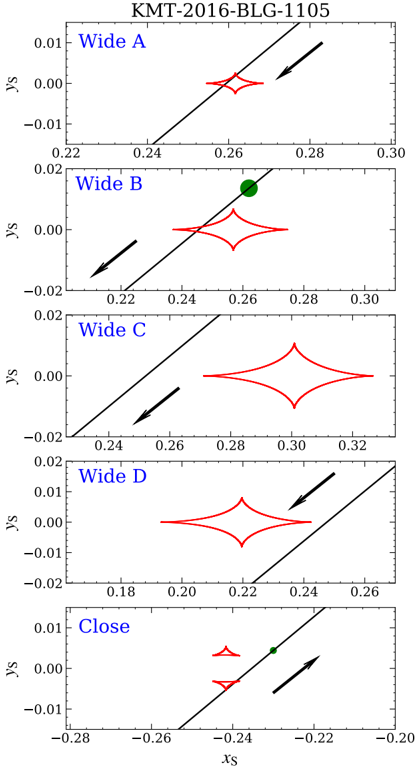
### Visual Description
## Chart: KMT-2016-BLG-1105 Microlensing Event Light Curves
### Overview
The image presents five separate light curves, each representing a different observation or "view" of the same microlensing event, KMT-2016-BLG-1105. Each light curve plots the change in position (Ys) against the change in position (Xs) over time, likely representing the deflection of light from a background star by a foreground lensing object. Each subplot is labeled "Wide A", "Wide B", "Wide C", "Wide D", and "Close", suggesting different observing conditions or telescopes. Each light curve also includes a linear trend line and a marker (green triangle or red arrow) indicating a specific point of interest.
### Components/Axes
* **Title:** KMT-2016-BLG-1105 (top-right)
* **X-axis Label:** Xs (bottom)
* **Y-axis Label:** Ys (left)
* **Subplot Labels:** Wide A, Wide B, Wide C, Wide D, Close (top-left of each subplot)
* **Linear Trend Lines:** Black lines in each subplot.
* **Data Points:** Red lines representing the light curve data.
* **Markers:** Green triangles and red arrows indicating specific points.
### Detailed Analysis or Content Details
**Wide A:**
* X-axis range: approximately 0.22 to 0.30
* Y-axis range: approximately -0.01 to 0.01
* The light curve shows a roughly symmetrical peak.
* A green triangle is located at approximately (Xs = 0.26, Ys = 0.00).
* The linear trend line has a positive slope.
**Wide B:**
* X-axis range: approximately 0.22 to 0.30
* Y-axis range: approximately -0.02 to 0.00
* The light curve shows a peak, but it is less pronounced than in Wide A.
* A green triangle is located at approximately (Xs = 0.26, Ys = -0.005).
* The linear trend line has a positive slope.
**Wide C:**
* X-axis range: approximately 0.24 to 0.32
* Y-axis range: approximately -0.02 to 0.02
* The light curve shows a clear peak.
* A green triangle is located at approximately (Xs = 0.28, Ys = 0.01).
* The linear trend line has a positive slope.
**Wide D:**
* X-axis range: approximately 0.18 to 0.26
* Y-axis range: approximately -0.01 to 0.01
* The light curve shows a peak.
* A green triangle is located at approximately (Xs = 0.22, Ys = -0.005).
* The linear trend line has a positive slope.
**Close:**
* X-axis range: approximately -0.28 to -0.20
* Y-axis range: approximately -0.01 to 0.01
* The light curve shows a peak.
* A red arrow is located at approximately (Xs = -0.24, Ys = 0.005).
* The linear trend line has a positive slope.
### Key Observations
* All light curves exhibit a peak, indicating a microlensing event.
* The peaks vary in amplitude and shape across the different observations.
* The green triangles consistently appear near the peak of the light curves.
* The "Close" light curve has a negative X-axis range, suggesting a different coordinate system or orientation.
* The linear trend lines are consistently positive, indicating a general upward trend in the data.
### Interpretation
The image depicts the light curves from a microlensing event, KMT-2016-BLG-1105. Microlensing occurs when a massive object (the lens) passes between a distant source star and the Earth, bending the light from the source and causing it to appear brighter. The different "Wide" and "Close" observations likely represent data taken with different telescopes or observing strategies, providing a more complete picture of the event.
The peaks in the light curves represent the maximum magnification of the source star due to the lensing effect. The variations in peak amplitude and shape suggest that the lensing object may have a complex structure or that the alignment between the source, lens, and Earth was not perfect. The green triangles likely mark the point of maximum magnification or a key feature in the light curve. The "Close" observation, with its negative X-axis values, may represent a different coordinate system or a zoomed-in view of the event.
The consistent positive slope of the linear trend lines suggests a systematic effect or a long-term trend in the data. This could be due to instrumental effects, atmospheric conditions, or a real physical phenomenon. Further analysis would be needed to determine the cause of this trend. The data suggests a microlensing event with variations in the lensing effect observed from different perspectives.
</details>
HJD ′ = 7548 . 0 and HJD ′ = 7548 . 3 . If the bump were
produced by a cusp approach with the upper triangular planetary caustic, there would be a dip before the bump, but the region before the bump is well covered by the KMTS and the KMTC data, which are consistent with the 1L1S model. Thus, the minor-image perturbation only has one solution.
Figure 12. Scatter plot of log q vs. ∆ ξ for KMT-2016-BLG-1105. The distribution is derived by inflating the error bars by a factor of √ 2 . 5 and then multiplying the resulting χ 2 by 2.5 for the plot. The colors are the same as those in Figure 3. 'A', 'B', 'C', and 'D' represent four local minima and the corresponding parameters are given in Table 9.
<details>
<summary>Image 12 Details</summary>
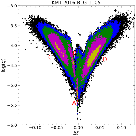
### Visual Description
## Scatter Plot: KMT-2016-BLG-1105 Microlensing Event
### Overview
This image presents a scatter plot visualizing data from the microlensing event KMT-2016-BLG-1105. The plot displays the relationship between Δξ (Delta xi) and log(q), with data points color-coded to represent different regions or phases of the event. The plot exhibits a characteristic "bow-tie" shape commonly observed in microlensing events with binary lenses.
### Components/Axes
* **Title:** KMT-2016-BLG-1105 (located at the top-center)
* **X-axis:** Δξ (Delta xi) - ranges approximately from -0.12 to 0.12.
* **Y-axis:** log(q) - ranges approximately from -6.0 to -3.0.
* **Data Points:** Numerous black dots representing individual data measurements.
* **Color Regions:** The data points are grouped into color-coded regions, labeled A, C, and D. The colors are as follows:
* A: Dark Red
* C: Magenta/Pink
* D: Yellow/Orange
* Green: Occupies a large central portion of the plot.
* Blue/Black: Forms the upper wings of the plot.
* **Labels:** A, C, and D are labels indicating specific regions within the plot.
### Detailed Analysis
The plot shows a concentration of data points around Δξ = 0, with log(q) values ranging from approximately -5.5 to -4.0. The data points are distributed in a roughly symmetrical pattern around the vertical axis (Δξ = 0).
* **Region A (Dark Red):** Located at the bottom center of the plot, around Δξ = 0 and log(q) ≈ -5.5. This region represents the peak of the microlensing event.
* **Region C (Magenta/Pink):** Situated on the left side of the plot, with Δξ values ranging from approximately -0.10 to -0.02 and log(q) values ranging from approximately -3.5 to -4.5.
* **Region D (Yellow/Orange):** Located on the right side of the plot, mirroring Region C, with Δξ values ranging from approximately 0.02 to 0.10 and log(q) values ranging from approximately -3.5 to -4.5.
* **Green Region:** Occupies the central area of the "bow-tie" shape, extending from Δξ ≈ -0.05 to 0.05 and log(q) ≈ -4.0 to -5.0.
* **Blue/Black Regions:** Form the upper wings of the plot, with Δξ values ranging from approximately -0.12 to 0.12 and log(q) values ranging from approximately -3.0 to -3.5. These regions represent the wings of the microlensing light curve.
The data points are densely packed within each colored region, indicating a high number of observations in those areas. The distribution of points suggests a smooth transition between the different regions.
### Key Observations
* The "bow-tie" shape is a strong indicator of a binary lens system.
* The symmetry of the plot around Δξ = 0 suggests a symmetrical lens configuration.
* The concentration of points in Region A indicates the peak magnification of the microlensing event.
* The distinct color-coded regions likely correspond to different phases or configurations of the binary lens system.
### Interpretation
This plot represents the light curve of a microlensing event caused by a binary lens system. Microlensing occurs when a foreground star passes in front of a background star, temporarily magnifying the background star's light. When the foreground star is actually a binary system, the resulting light curve exhibits characteristic features, such as the "bow-tie" shape observed here.
The different color-coded regions likely represent different configurations of the binary lens system during the event. Region A corresponds to the peak magnification, while Regions C and D represent the wings of the light curve, where the magnification is lower. The green region represents intermediate magnification levels.
The symmetry of the plot suggests that the binary lens system is aligned in a way that produces a symmetrical magnification pattern. The data suggests the presence of two distinct lenses within the foreground system, causing the observed distortions in the light curve. The log(q) parameter represents the mass ratio of the two lenses. The shape and distribution of the data points provide valuable information about the masses, separation, and relative positions of the two lenses. This type of analysis is crucial for detecting and characterizing exoplanets orbiting stars in binary systems.
</details>
For the four 'Wide' solutions, the 'Wide A' and 'Wide B' solutions have a source crossing the planetary caustic, and the 'Wide C' and 'Wide D' solutions that contain a source that passes to one side or the other of the planetary caustic. This topology is qualitatively similar to the topology of OGLE-2017-BLG-0173 (Hwang et al. 2018a). We thus also investigate the parameter space by a 'hotter' MCMC with the error bar inflated by a factor of √ 2 . 5 . The resulting scatter plot is shown in Figure 12, from which we find that the topology of KMT-2016-BLG-1105 has differences in three aspects from the topology of OGLE-2017-BLG-0173. First, for the two solutions in which the source passes to one side or the other of the planetary caustic, OGLE-2017-BLG-0173 has caustic crossings and the source is comparable to the size of the planetary caustic, but in the present case, the source does not cross the caustic. Second, for the solution in which the source passes directly over the planetary caustic, the source is much larger than the planetary caustics in the case of OGLE2017-BLG-0173, while the source of KMT-2016-BLG-1105 is smaller than the caustic. Third, OGLE-2017-BLG-0173
exhibits a bimodal minimum when the source passes directly over the caustic, and the mass-ratio difference between the two local minima is ∆log q < 0 . 1 . The corresponding solutions for KMT-2016-BLG-1105, the 'Wide A' and 'Wide B' solutions, have ∆log q ∼ 1 . We note that the 'Wide A' and 'Wide B' solutions have ∆ ξ ∼ 0.00 and -0.01, respectively. Considering the approximate symmetry with respect to ∆ ξ , one might expect an additional minimum that has ∆ ξ ∼ 0 . 01 and a similar log q as the log q of the 'Wide B' solution. However, such a potential solution 'disappeared' from the numerical analysis. Because the trajectories of the 'Wide' B solution and the putative minimum at ∆ ξ ∼ 0 . 01 should be almost symmetric with respect to the center of the caustics, their corresponding planetary signals should also be almost symmetric. As shown in Figure 10, the 'Wide B' solution drops rapidly during the caustic exit, followed by a dip, so the putative minimum at ∆ ξ ∼ 0 . 01 should contain a dip followed by a sudden rise during the caustic entry, which is not supported by the KMTC and KMTS data. Thus, in Figure 12 this topology is absorbed into the MCMC chain of the 'Wide D' solution and there is no new discrete solution.
We also check whether the bump-type anomaly can be fitted by a 1L2S model. Table 8 lists the 1L2S parameters. We find that the best-fit 1L2S model is disfavored by ∆ χ 2 = 12 . 0 compared to the best-fit 2L1S model. The bestfit 1L2S model has ρ 2 = 0 . 0018 . We note that the flux ratio is q f,I ∼ 2 × 10 -3 , corresponding to a magnitude difference of 6.7 mag. According to Section 5, the primary source lies 4.1 mag below the red giant clump, so the putative source companion would have an absolute magnitude of M I, 2 ∼ 10 . 7 mag, corresponding to an angular source radius of θ ∗ , 2 ∼ 0 . 1 µ as. This yields the lens-source relative proper motion of µ rel = θ ∗ , 2 /ρ 2 /t E ∼ 0 . 5 mas yr -1 , which is lower than the typical µ rel of bulge microlensing events (See Figure 2 of Zhu et al. (2017) for examples). However, a model with ρ 2 = 0 is only disfavored by ∆ χ 2 = 1 , so any reasonable µ rel is only disfavored by ∆ χ 2 < 1 . Thus, while the planetary model is strongly favored, there is a possibility that the anomaly is caused by a second source.
With high-order effects, we find that ∆ χ 2 < 1 and the 1 σ uncertainty of parallax is > 0 . 9 at all directions, so the constraint on π E is not useful.
## 5. SOURCE AND LENS PROPERTIES
## 5.1. Preamble
Combining Equations (1) and (7), the mass M L and distance D L of a lens system are related to the angular Einstein radius θ E and the microlensing parallax π E by (Gould 1992, 2000)
<!-- formula-not-decoded -->
<details>
<summary>Image 13 Details</summary>
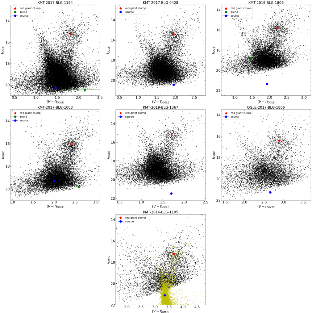
### Visual Description
\n
## Scatter Plots: Microlensing Event Color-Magnitude Diagrams
### Overview
The image contains nine separate scatter plots, each representing a color-magnitude diagram for a microlensing event. Each plot displays the relationship between two color indices (V-I or V-IOGLE, V-K) and magnitude (IOGLE or IkmTc). The plots are arranged in a 3x3 grid. Each plot includes data points representing stars, with different symbols indicating the "red giant clump", "blend", and "source" stars.
### Components/Axes
Each plot shares the following components:
* **X-axis:** Color index (V-I, V-IOGLE, or V-K). Scales range approximately from 0.5 to 4.5, depending on the plot.
* **Y-axis:** Magnitude (IOGLE or IkmTc). Scales range approximately from 14 to 22, depending on the plot.
* **Title:** Identifies the microlensing event (e.g., "KMT-2017-BLG-1194").
* **Legend:** Located in the top-left corner of each plot, defining the symbols used for "red giant clump" (red star), "blend" (green triangle), and "source" (purple circle).
The specific plots and their titles are:
1. KMT-2017-BLG-1194
2. KMT-2017-BLG-0428
3. KMT-2019-BLG-1806
4. KMT-2017-BLG-1003
5. KMT-2019-BLG-1367
6. OGLE-2017-BLG-1806
7. KMT-2017-BLG-0206
8. KMT-2016-BLG-1105
9. KMT-2017-BLG-393
### Detailed Analysis or Content Details
Each plot shows a concentration of points representing stars, forming a general trend. The "red giant clump" stars appear as a distinct concentration, while "blend" and "source" stars are often highlighted with individual markers.
Here's a breakdown of the approximate data points for each plot, focusing on the highlighted "source" stars (purple circles):
1. **KMT-2017-BLG-1194:** Source star at approximately (V-I = 1.8, IOGLE = 16.5).
2. **KMT-2017-BLG-0428:** Source star at approximately (V-IOGLE = 1.9, IOGLE = 17.5).
3. **KMT-2019-BLG-1806:** Source star at approximately (V-I = 2.8, IOGLE = 18.5).
4. **KMT-2017-BLG-1003:** Source star at approximately (V-IOGLE = 2.2, IOGLE = 17.0).
5. **KMT-2019-BLG-1367:** Source star at approximately (V-IOGLE = 1.7, IOGLE = 18.0).
6. **OGLE-2017-BLG-1806:** Source star at approximately (V-K = 3.1, IkmTc = 16.0).
7. **KMT-2017-BLG-0206:** No clear source star is visible.
8. **KMT-2016-BLG-1105:** Source star at approximately (V-K = 3.8, IkmTc = 16.5).
9. **KMT-2017-BLG-393:** Source star at approximately (V-K = 3.9, IkmTc = 17.0).
The "blend" stars (green triangles) are scattered across the plots, generally at lower magnitudes than the "red giant clump" stars. The "red giant clump" stars (red stars) form a relatively tight cluster in each plot.
### Key Observations
* The source stars are consistently highlighted, suggesting they are the primary objects of interest in these microlensing events.
* The color-magnitude relationships vary slightly between the different events, as indicated by the different positions of the star clusters.
* The plots demonstrate a clear separation between the red giant clump, blend, and source stars based on their color and magnitude.
* The data points are densely packed, indicating a large number of stars observed in each field.
### Interpretation
These color-magnitude diagrams are used to study microlensing events, which occur when a massive object (like a star or black hole) passes between Earth and a distant star, magnifying the light from the distant star. The different star populations ("red giant clump", "blend", "source") are identified based on their color and magnitude, allowing astronomers to model the microlensing event and infer properties of the lensing object.
The variations in the diagrams likely reflect differences in the line of sight, the distance to the stars, and the composition of the stellar populations in each field. The highlighted "source" stars represent the stars being lensed, and their positions in the diagrams provide information about their intrinsic properties. The "blend" stars are stars that lie along the line of sight to the source star and contribute to the observed light, while the "red giant clump" stars are a common population of stars in the Milky Way.
The consistent use of color-magnitude diagrams across these events suggests a standardized approach to analyzing microlensing data. The plots provide a visual representation of the data, allowing astronomers to identify and characterize the different star populations and model the microlensing event.
</details>
(V-I)KMTC
Figure 13. Color magnitude diagrams for the seven planetary events analyzed in this paper. The first five CMDs are constructed using the OGLE-III star catalog (Szyma´ nski et al. 2011), and the other two CMDs are constructed using the KMTC pyDIA photometry reduction. For each panel, the red asterisk and the blue dot are shown as the centroid of the red giant clump and the microlensed source star, respectively. The three green dots on the CMDs of KMT-2017-BLG-1194, KMT-2019-BLG-1806, and KMT-2017-BLG-1003 represent the blended light. For the bottom panel, the yellow dots represent the HST CMD of Holtzman et al. (1998) whose red-clump centroid has been matched to that of KMTC using ( V -I, I ) cl , HST = (1 . 62 , 15 . 15) (Bennett et al. 2008).
Table 10. CMDparameters, θ ∗ , θ E and µ rel for the five 'dip' planetary events
| Parameter | KB171194 | KB170428 | KB191806 | KB171003 | KB171003 | KB191367 |
|---------------------|-------------------|-------------------|-------------------|-------------------|-------------------|-------------------|
| | | | | Inner | Outer | |
| ( V - I ) cl | 1 . 82 ± 0 . 01 | 1 . 95 ± 0 . 01 | 2 . 23 ± 0 . 01 | 2 . 39 ± 0 . 01 | ← | 1 . 70 ± 0 . 01 |
| I cl | 15 . 25 ± 0 . 01 | 15 . 39 ± 0 . 01 | 15 . 79 ± 0 . 02 | 16 . 04 ± 0 . 01 | ← | 15 . 13 ± 0 . 01 |
| I cl , 0 | 14 . 26 ± 0 . 04 | 14 . 36 ± 0 . 04 | 14 . 39 ± 0 . 04 | 14 . 34 ± 0 . 04 | ← | 14 . 37 ± 0 . 04 |
| ( V - I ) S | 1 . 47 ± 0 . 07 | 1 . 95 ± 0 . 04 | 1 . 93 ± 0 . 03 | 2 . 00 ± 0 . 02 | ← | 1 . 70 ± 0 . 03 |
| I S | 20 . 28 ± 0 . 08 | 20 . 43 ± 0 . 05 | 21 . 35 ± 0 . 07 | 19 . 30 ± 0 . 04 | 19 . 30 ± 0 . 04 | 21 . 47 ± 0 . 13 |
| ( V - I ) S , 0 | 0 . 71 ± 0 . 08 | 1 . 06 ± 0 . 05 | 0 . 76 ± 0 . 05 | 0 . 67 ± 0 . 04 | ← | 1 . 06 ± 0 . 04 |
| I S , 0 | 19 . 29 ± 0 . 09 | 19 . 40 ± 0 . 07 | 19 . 95 ± 0 . 08 | 17 . 60 ± 0 . 06 | 17 . 60 ± 0 . 06 | 20 . 71 ± 0 . 14 |
| θ ∗ ( µ as) | 0 . 448 ± 0 . 038 | 0 . 578 ± 0 . 034 | 0 . 345 ± 0 . 020 | 0 . 942 ± 0 . 046 | 0 . 942 ± 0 . 046 | 0 . 316 ± 0 . 023 |
| θ E (mas) | > 0 . 17 | > 0 . 09 | > 0 . 19 | > 0 . 14 | 0 . 180 ± 0 . 041 | > 0 . 06 |
| µ rel ( masyr - 1 ) | > 1 . 3 | > 0 . 74 | > 0 . 51 | > 2 . 0 | 2 . 56 ± 0 . 58 | > 0 . 53 |
NOTE- ( V - I ) cl , 0 = 1 . 06 ± 0 . 03 . Event names are abbreviations, e.g., KMT-2017-BLG-1194 to KB171194.
Table 11. CMDparameters, θ ∗ , θ E and µ rel for OGLE-2017-BLG-1806.
| Parameter | Close A | Close A | Close B | Close B | Wide | Wide |
|---------------------|----------------------------|----------------------------|----------------------------|----------------------------|-------------------|-------------------|
| | u 0 > 0 | u 0 < 0 | u 0 > 0 | u 0 < 0 | u 0 > 0 | u 0 < 0 |
| ( V - I ) cl | 2 . 89 ± 0 . 01 | ← | ← | ← | ← | ← |
| I cl | 16 . 42 ± 0 . 02 | ← | ← | ← | ← | ← |
| I cl , 0 | 14 . 33 ± 0 . 04 | ← | ← | ← | ← | ← |
| ( V - I ) S | 2 . 66 ± 0 . 03 | ← | ← | ← | ← | ← |
| I S | 21 . 12 ± 0 . 07 | 21 . 07 ± 0 . 07 | 21 . 10 ± 0 . 08 | 21 . 10 ± 0 . 08 | 21 . 03 ± 0 . 07 | 21 . 08 ± 0 . 07 |
| ( V - I ) S , 0 | 0 . 83 ± 0 . 04 | ← | ← | ← | ← | ← |
| I S , 0 | 19 . 03 ± 0 . 08 | 18 . 98 ± 0 . 08 | 19 . 01 ± 0 . 09 | 19 . 01 ± 0 . 09 | 18 . 94 ± 0 . 08 | 18 . 99 ± 0 . 08 |
| θ ∗ ( µ as) | 0 . 561 ± 0 . 031 | 0 . 574 ± 0 . 031 | 0 . 566 ± 0 . 033 | 0 . 566 ± 0 . 033 | 0 . 584 ± 0 . 032 | 0 . 571 ± 0 . 032 |
| θ E (mas) | 0 . 322 +0 . 083 - 0 . 145 | 0 . 314 +0 . 087 - 0 . 138 | 0 . 377 +0 . 120 - 0 . 157 | 0 . 343 +0 . 105 - 0 . 141 | > 0 . 21 | > 0 . 24 |
| µ rel ( masyr - 1 ) | 1 . 69 +0 . 45 - 0 . 77 | 1 . 72 +0 . 49 - 0 . 76 | 1 . 98 +0 . 64 - 0 . 84 | 2 . 08 +0 . 65 - 0 . 87 | > 1 . 2 | > 1 . 3 |
Table 12. CMDparameters, θ ∗ , θ E and µ rel for KMT-2016-BLG-1105.
| | Wide A | Wide B | Wide C | Wide D | Close |
|---------------------|-------------------|-------------------|-------------------|-------------------|-------------------|
| I cl | 17 . 20 ± 0 . 01 | ← | ← | ← | ← |
| I cl , 0 | 14 . 39 ± 0 . 04 | ← | ← | ← | ← |
| I S | 21 . 09 ± 0 . 08 | 21 . 20 ± 0 . 05 | 21 . 22 ± 0 . 11 | 21 . 22 ± 0 . 11 | 21 . 27 ± 0 . 06 |
| ( V - I ) S , 0 | 0 . 74 ± 0 . 07 | 0 . 75 ± 0 . 07 | 0 . 75 ± 0 . 07 | 0 . 75 ± 0 . 07 | 0 . 75 ± 0 . 07 |
| I S , 0 | 18 . 28 ± 0 . 09 | 18 . 39 ± 0 . 07 | 18 . 41 ± 0 . 12 | 18 . 41 ± 0 . 12 | 18 . 46 ± 0 . 07 |
| θ ∗ ( µ as) | 0 . 732 ± 0 . 057 | 0 . 702 ± 0 . 051 | 0 . 696 ± 0 . 061 | 0 . 696 ± 0 . 061 | 0 . 680 ± 0 . 050 |
| θ E (mas) | > 0 . 31 | 0 . 240 ± 0 . 070 | > 0 . 15 | > 0 . 13 | 0 . 907 ± 0 . 182 |
| µ rel ( masyr - 1 ) | > 2 . 9 | 2 . 07 ± 0 . 62 | > 1 . 3 | > 1 . 1 | 7 . 65 ± 1 . 54 |
To obtain the angular Einstein radius through θ E = θ ∗ /ρ , we first estimate the angular source radius θ ∗ by locating the source on a color-magnitude diagram (CMD, Yoo et al. 2004). For each event, we construct a V -I versus I CMD using the ambient stars of the OGLE-III catalog (Szyma´ nski et al. 2011) or the KMTC images with the pyDIA reductions. See Figure 13 for the CMDs of the seven planetary events. Weestimate the centroid of the red giant clump as ( V -I, I ) cl from CMDs and adopt the de-reddened color and magnitude of the red giant clump, ( V -I, I ) cl , 0 , from Bensby et al. (2013) and Table 1 of Nataf et al. (2013). We obtain the source apparent magnitude from the light-curve analysis of Section 4, and the source color by a regression of the KMTC V versus I flux with the change of the lensing magnification.
We find that the V -band observations of KMT-2016-BLG1105 have insufficient signal-to-noise ratio to determine the source color, so we estimate the source color by the Hubble Space Telescope ( HST ) CMD of Holtzman et al. (1998) (see Section 5.7 for details). Finally, using the color/surfacebrightness relation of Adams et al. (2018), we obtain the angular source radius θ ∗ . Tables 10, 11 and 12 present the CMD values and ( θ ∗ , θ E , µ rel ) from the procedures above.
Because the blended light could provide additional constraints on the lens properties (e.g., the upper limits for the lens brightness), we also check the brightness and the astrometric alignment of the baseline object. For KMT-2017BLG-0428 and KMT-2019-BLG-1806, we adopt the i ′ -band baseline images taken by the 3.6m Canada-France-Hawaii Telescope (CFHT) from 2020 to 2022, whose seeing FWHM is 0 . ′′ 55 -0 . ′′ 70 . For the other five events which do not have any CFHT image, we check the baseline objects from the KMTC pyDIA reduction, whose seeing FWHM is about 1 . ′′ 0 .
Because none of the seven planetary events have simultaneous measurements of π E and θ E at the > 3 σ level, the lens masses and distances cannot be directly determined by Equa- tion (18). We conduct a Bayesian analysis using a Galactic model to estimate the lens properties. The Galactic model and the procedures we adopt are the same as described in Zang et al. (2021b). We refer the reader to that work for details. The only exception is that we include upper limits of the lens light, I L , limit , from the analysis of the blended light. We adopt the mass-luminosity relation of Wang et al. (2018),
<!-- formula-not-decoded -->
where M I is the absolute magnitude in the I band, and we reject trial events for which the lens properties obey
<!-- formula-not-decoded -->
where A I,D L is the extinction at D L . We adopt an extinction curve with a scale height of 120 pc. For the five events with OGLE CMDs, the total extinction is derived from the CMD analysis, A I = I cl -I cl , 0 . For the other two events with KMTC CMDs, we adopt the extinction in the K band from Gonzalez et al. (2012) and A I = 7 . 26 A K from Nataf et al. (2016).
Table 13 presents the resulting Bayesian estimates of the host mass M host , the planet mass M planet , the lens distance D L , the projected planet-host separation a ⊥ and the lenssource relative proper motion µ rel . For events with multiple solutions, we show the results for each solution and the 'combined results' of combining all solutions weighted by their Galactic-model likelihood and exp( -∆ χ 2 / 2) , where ∆ χ 2 is the χ 2 difference compared to the best-fit solution. Here the Galactic-model likelihood represents the total weight for the simulated events given the error distributions of t E , θ E and π E . See Equation (16) of Zang et al. (2021b) for the weight procedures.
We do not adopt the 'combined results' as the final physical parameters but just show them for consideration, be-
Table 13. Physical parameters of the six planetary events from a Bayesian analysis.
| Event | Solution | Physical Properties | Physical Properties | Physical Properties | Physical Properties | Physical Properties | Relative Weights | Relative Weights |
|----------|---------------------|-------------------------------|--------------------------|-------------------------|-------------------------|-------------------------|--------------------|--------------------|
| | | M host [ M ] | M planet [ M ⊕ ] | D L [kpc] | a ⊥ [au] | µ rel [ masyr - 1 ] | Gal.Mod. | χ 2 |
| KB171194 | | 0 . 41 +0 . 23 - 0 . 19 | 3 . 54 +1 . 95 - 1 . 63 | 4 . 24 +2 . 16 - 1 . 71 | 1 . 78 +0 . 45 - 0 . 46 | 4 . 29 +2 . 50 - 1 . 66 | ... | ... |
| KB170428 | Inner | 0 . 34 +0 . 22 - 0 . 17 | 5 . 63 +3 . 59 - 2 . 85 | 5 . 40 +1 . 82 - 2 . 60 | 1 . 78 +0 . 54 - 0 . 58 | 3 . 27 +2 . 26 - 1 . 32 | 0.99 | 1.00 |
| KB170428 | Outer | 0 . 34 +0 . 22 - 0 . 17 | 5 . 55 +3 . 53 - 2 . 81 | 5 . 40 +1 . 82 - 2 . 60 | 1 . 85 +0 . 55 - 0 . 60 | 3 . 28 +2 . 24 - 1 . 34 | 1.00 | 0.95 |
| KB170428 | Combined | 0 . 34 +0 . 22 - 0 . 17 | 5 . 59 +3 . 57 - 2 . 83 | 5 . 40 +1 . 82 - 2 . 60 | 1 . 81 +0 . 55 - 0 . 59 | 3 . 27 +2 . 26 - 1 . 32 | ... | ... |
| KB191806 | Inner ( u 0 > 0 ) | 0 . 75 +0 . 24 - 0 . 25 | 4 . 67 +1 . 52 - 1 . 52 | 6 . 62 +0 . 72 - 1 . 93 | 2 . 87 +0 . 64 - 0 . 66 | 1 . 17 +0 . 70 - 0 . 34 | 1.00 | 0.70 |
| KB191806 | Inner ( u 0 < 0 ) | 0 . 74 +0 . 25 - 0 . 26 | 4 . 47 +1 . 56 - 1 . 52 | 6 . 63 +0 . 73 - 2 . 01 | 2 . 85 +0 . 66 - 0 . 70 | 1 . 11 +0 . 74 - 0 . 34 | 0.84 | 0.58 |
| KB191806 | Outer ( u 0 > 0 ) | 0 . 73 +0 . 25 - 0 . 26 | 4 . 63 +1 . 60 - 1 . 64 | 6 . 68 +0 . 72 - 1 . 97 | 3 . 11 +0 . 73 - 0 . 79 | 1 . 13 +0 . 70 - 0 . 36 | 0.98 | 0.82 |
| KB191806 | Outer ( u 0 < 0 ) | 0 . 75 +0 . 24 - 0 . 25 | 4 . 79 +1 . 56 - 1 . 60 | 6 . 62 +0 . 74 - 2 . 09 | 3 . 17 +0 . 70 - 0 . 75 | 1 . 15 +0 . 74 - 0 . 36 | 0.98 | 1.00 |
| KB191806 | Combined | 0 . 74 +0 . 25 - 0 . 25 | 4 . 67 +1 . 56 - 1 . 60 | 6 . 64 +0 . 72 - 2 . 01 | 3 . 02 +0 . 70 - 0 . 73 | 1 . 13 +0 . 74 - 0 . 34 | ... | ... |
| KB171003 | Inner | 0 . 37 +0 . 32 - 0 . 19 | 6 . 75 +5 . 79 - 3 . 44 | 7 . 03 +0 . 61 - 0 . 74 | 1 . 54 +0 . 38 - 0 . 37 | 3 . 55 +0 . 88 - 0 . 84 | 1.00 | 0.90 |
| KB171003 | Outer | 0 . 27 +0 . 26 - 0 . 13 | 3 . 72 +3 . 71 - 1 . 80 | 7 . 16 +0 . 61 - 0 . 65 | 1 . 25 +0 . 27 - 0 . 25 | 2 . 75 +0 . 56 - 0 . 54 | 0.74 | 1.00 |
| KB171003 | Combined | 0 . 32 +0 . 31 - 0 . 17 | 5 . 19 +5 . 39 - 2 . 80 | 7 . 09 +0 . 61 - 0 . 70 | 1 . 38 +0 . 39 - 0 . 32 | 3 . 11 +0 . 94 - 0 . 72 | ... | ... |
| KB191367 | Inner | 0 . 25 +0 . 16 - 0 . 13 | 4 . 06 +2 . 56 - 2 . 08 | 4 . 68 +2 . 44 - 2 . 10 | 1 . 67 +0 . 49 - 0 . 55 | 3 . 92 +2 . 57 - 1 . 71 | 1.00 | 1.00 |
| KB191367 | Outer | 0 . 25 +0 . 16 - 0 . 13 | 4 . 12 +2 . 58 - 2 . 10 | 4 . 67 +2 . 45 - 2 . 10 | 1 . 73 +0 . 51 - 0 . 57 | 3 . 89 +2 . 55 - 1 . 71 | 0.96 | 0.90 |
| KB191367 | Combined | 0 . 25 +0 . 16 - 0 . 13 | 4 . 08 +2 . 58 - 2 . 08 | 4 . 67 +2 . 45 - 2 . 10 | 1 . 70 +0 . 50 - 0 . 56 | 3 . 91 +2 . 56 - 1 . 71 | ... | ... |
| OB171806 | Close A ( u 0 > 0 ) | 0 . 44 +0 . 33 - 0 . 23 | 5 . 87 +4 . 43 - 3 . 04 | 6 . 60 +0 . 65 - 1 . 06 | 1 . 84 +0 . 44 - 0 . 51 | 1 . 95 +0 . 46 - 0 . 54 | 0.85 | 0.90 |
| OB171806 | Close A ( u 0 < 0 ) | 0 . 33 +0 . 33 - 0 . 16 | 4 . 83 +4 . 83 - 2 . 44 | 6 . 17 +0 . 92 - 1 . 57 | 1 . 69 +0 . 46 - 0 . 43 | 2 . 13 +0 . 56 - 0 . 58 | 1.00 | 1.00 |
| OB171806 | Close B ( u 0 > 0 ) | 0 . 44 +0 . 39 - 0 . 26 | 2 . 40 +2 . 24 - 1 . 48 | 5 . 95 +1 . 11 - 2 . 13 | 1 . 89 +0 . 58 - 0 . 62 | 2 . 39 +0 . 78 - 0 . 70 | 0.21 | 10 - 3 . 1 |
| OB171806 | Close B ( u 0 < 0 ) | 0 . 48 +0 . 35 - 0 . 26 | 2 . 68 +1 . 96 - 1 . 48 | 6 . 53 +0 . 69 - 1 . 41 | 1 . 91 +0 . 50 - 0 . 58 | 2 . 09 +0 . 58 - 0 . 60 | 0.16 | 10 - 3 . 2 |
| OB171806 | Wide ( u 0 > 0 ) | 0 . 34 +0 . 31 - 0 . 16 | 5 . 47 +4 . 87 - 2 . 60 | 3 . 01 +2 . 22 - 1 . 09 | 2 . 53 +1 . 06 - 0 . 78 | 4 . 92 +1 . 74 - 1 . 94 | 10 - 1 . 5 | 10 - 1 . 8 |
| OB171806 | Wide ( u 0 < 0 ) | 0 . 41 +0 . 23 - 0 . 17 | 4 . 87 +2 . 72 - 2 . 00 | 2 . 87 +1 . 13 - 0 . 86 | 2 . 82 +0 . 85 - 0 . 78 | 5 . 48 +1 . 30 - 1 . 42 | 0.24 | 10 - 1 . 8 |
| OB171806 | Combined | 0 . 38 +0 . 34 - 0 . 20 | 5 . 27 +4 . 71 - 2 . 72 | 6 . 40 +0 . 77 - 1 . 51 | 1 . 75 +0 . 46 - 0 . 47 | 2 . 05 +0 . 52 - 0 . 56 | ... | ... |
| KB161105 | Wide A | 0 . 43 +0 . 22 - 0 . 20 | 0 . 92 +0 . 44 - 0 . 44 | 3 . 79 +1 . 38 - 1 . 44 | 2 . 93 +0 . 69 - 0 . 91 | 6 . 48 +2 . 08 - 1 . 30 | 0.37 | 1.00 |
| KB161105 | Wide B | 0 . 37 +0 . 31 - 0 . 21 | 4 . 67 +3 . 75 - 2 . 64 | 7 . 12 +0 . 65 - 1 . 10 | 2 . 03 +0 . 52 - 0 . 53 | 2 . 29 +0 . 62 - 0 . 56 | 1.00 | 0.32 |
| KB161105 | Wide C | 0 . 43 +0 . 27 - 0 . 23 | 12 . 14 +7 . 63 - 6 . 31 | 5 . 42 +1 . 85 - 2 . 33 | 2 . 63 +0 . 79 - 0 . 83 | 3 . 97 +2 . 68 - 1 . 58 | 0.66 | 0.11 |
| KB161105 | Wide D | 0 . 44 +0 . 27 - 0 . 23 | 9 . 51 +5 . 75 - 4 . 87 | 5 . 28 +1 . 92 - 2 . 23 | 2 . 56 +0 . 73 - 0 . 74 | 4 . 11 +2 . 64 - 1 . 56 | 0.64 | 0.26 |
| KB161105 | Close | 0 . 43 +0 . 18 - 0 . 18 | 1 . 32 +0 . 56 - 0 . 56 | 3 . 27 +1 . 28 - 1 . 15 | 2 . 26 +0 . 51 - 0 . 69 | 6 . 74 +1 . 74 - 1 . 58 | 0.29 | 0.17 |
| KB161105 | Combined | 0 . 41 +0 . 25 - 0 . 21 | 2 . 32 +7 . 43 - 1 . 56 | 5 . 08 +2 . 24 - 2 . 18 | 2 . 44 +0 . 88 - 0 . 75 | 4 . 68 +2 . 76 - 2 . 50 | ... | ... |
NOTE-The combined solution is obtained by a combination of all solutions weighted by the probability for the Galactic model (Gal.Mod.) and exp( -∆ χ 2 / 2) .
cause there is no conclusion about how to combine degenerate solutions. We note that the exp( -∆ χ 2 / 2) probability might be suffered from systematic errors of the observed data. However, the weight from ∆ χ 2 only has minor effects on the 'combined results'. Except for KMT-2016-BLG1105 the degenerate solutions have similar physical interpretations and except for OGLE-2017-BLG-1806 the ∆ χ 2 is small, but for OGLE-2017-BLG-1806 the 'combined results' are already dominated by the 'Close A' solutions due to their Galactic-model likelihoods. Due to similar reasons, whether to include the phase-space factors also has a minor impact on the 'combined results'.
## 5.2. KMT-2017-BLG-1194
The corresponding CMD shown in Figure 13 is constructed from the OGLE-III field stars within 240 ′′ centered on the event. The baseline object has ( V, I ) base = (21 . 343 ± 0 . 085 , 19 . 608 ± 0 . 051) , yielding a blend of ( V -I, I ) B = (2 . 15 ± 0 . 39 , 20 . 45 ± 0 . 14) . We display the blend on the CMD. The source position measured by the difference imaging analysis is displaced from the baseline object by ∆ θ ( N,E ) = ( -26 , 41) mas. We estimate the error of the baseline position by the fractional astrometric error being equal to the fractional photometric error (Jung et al. 2020), which yields σ ast = 0 . 39 σ I FWHM = 20 mas. We note that the astrometric error should be underestimated due to the mottled background from unresolved stars and other systematic errors, but the whole astrometric error should be not more than twice our estimate. Thus, the baseline object is astrometrically consistent with the source and the lens within 2 σ . The blend does not have a useful color constraint. We adopt the 3 σ upper limit of the blended light, I L , limit = 20 . 03 , as the upper limit of the lens brightness.
As given in Table 13, the preferred host star is an M dwarf located in the Galactic disk, and the planet is probably a super-Earth beyond the snow line of the lens system (assuming a snow line radius a SL = 2 . 7( M/M ) au, Kennedy & Kenyon 2008).
## 5.3. KMT-2017-BLG-0428
The corresponding CMD shown in Figure 13 consists of the OGLE-III field stars within 150 ′′ centered on the event. The baseline object on the CFHT images has I base = 20 . 056 ± 0 . 063 , with an astrometric offset of ∆ θ ( N,E ) = (6 , -2) mas and an astrometric error of σ ast ∼ 5 mas. Thus, the baseline object is astrometrically consistent with the source at about 1 σ . Because the CFHT images do not contain color information, we do not display the blend on the CMD. We also adopt the 3 σ upper limit of the blended light, I L , limit = 20 . 81 , as the upper limit of the lens brightness.
As shown in Table 13, the Bayesian analysis indicates another cold super-Earth orbiting an M dwarf.
## 5.4. KMT-2019-BLG-1806
The CMD of this event is constructed from the OGLEIII field stars within 150 ′′ centered on the event, shown in Figure 13. The baseline object on the KMTC images has ( V, I ) base = (20 . 155 ± 0 . 125 , 18 . 685 ± 0 . 076) . We plot the blend on the CMD and find that the blend probably belongs to the foreground main-sequence branch and thus could be the lens. However, the astrometric offset is ∆ θ ( N,E ) = (433 , -76) mas and ∆ θ ( N,E ) = (416 , -96) mas on the CFHT and KMTC images, respectively, so the majority of the blended light is unrelated to the lens. We adopt the median value of the blended light, I L , limit = 18 . 8 , as the upper limit of the lens brightness.
The results of the Bayesian analysis are given in Table 13. The planet is another cold super-Earth, and the preferred host is a K dwarf.
## 5.5. KMT-2017-BLG-1003
We use the OGLE-III field stars within 180 ′′ centered on the event to build the CMD. Combining the measured ρ from the light-curve analysis, we obtain θ E = 0 . 180 ± 0 . 041 mas for the 'Outer' solution and θ E > 0 . 14 mas ( 3 σ ) for the 'Inner' solution. The KMTNet baseline object has ( V, I ) base = (20 . 968 ± 0 . 046 , 18 . 780 ± 0 . 028) , corresponding to a blend of ( V -I, I ) B = (2 . 54 ± 0 . 20 , 19 . 83 ± 0 . 10) , and we display the blend on the CMD. The source-baseline astrometric offset is ∆ θ ( N,E ) = ( -64 , -77) mas, with an astrometric error of σ ast ∼ 12 mas, implying that most of the blend light should be unrelated to the event. We adopt the median value of the blended light, I L , limit = 19 . 83 , as the upper limit of the lens brightness.
The Bayesian analysis shows that the host star is probably an M dwarf located in the Galactic bulge. Again, the preferred planet is a cold super-Earth.
## 5.6. KMT-2019-BLG-1367
In Figure 13, we display the position of the source on the CMDof stars within 180 ′′ around the source. On the KMTC images, there is no star within 1 . ′′ 4 around the source position. We thus adopt the detection limit of the KMTC images, I = 21 . 0 , as the upper limit of the baseline brightness, yielding the 3 σ upper limit of the blended light, I L , limit = 21 . 6 . Applying Equations (19) and (20) and assuming D L < 8 kpc, this flux constraint corresponds to an upper limit of the lens mass of 0 . 6 M .
As shown in Table 13, the Bayesian estimate shows another cold super-Earth orbiting an M dwarf.
## 5.7. OGLE-2017-BLG-1806
The CMD of this event is constructed from KMTC field stars within a 300 ′′ square centered on the event position. The baseline object, ( V, I ) base = (22 . 300 ± 0 . 308 , 20 . 042 ±
0 . 128) , is displaced from the source by 835 mas. Thus, most of the blend light should be unrelated to the event. We do not show the blend on the CMD and adopt the median value of the blended light, I L , limit = 20 . 5 , as the upper limit of the lens brightness.
The results of the Bayesian analysis are presented in Table 13, and all solutions indicate a cold super-Earth orbiting a low-mass star. The constraints on π E , ⊥ from the lightcurve analysis are useful. The 'Wide' solution has a relatively large θ E , with a 2 σ lower limit of 0 . 60 mas and the best-fit value of ∼ 1 . 1 mas, so the corresponding lens system is located in the Galactic disk. Then, the 'Wide ( u 0 > 0 )' solution has π E , ⊥ < 0 and thus a lens velocity in Galactic coordinates of v ∼ 100 km s -1 , so this solution is strongly disfavored. For the two 'Close' solutions, both the π E , ⊥ < 0 solutions are slightly disfavored and have relatively higher probabilities of a bulge lens system.
For the 'Wide' solution, the predicted apparent magnitude of the lens system is fainter than the source by ∼ 0 . 8 mag in the H band. In the case of OGLE-2012-BLG-0950, the source and the lens have roughly equal brightness and were resolved by the Keck AO imaging and the HST imaging when they were separated by about 34 mas (Bhattacharya et al. 2018). For OGLE-2017-BLG-1806, we estimate that resolving the lens and source probably requires a separation of 45 mas for the 'Wide' solution. We note that the proper motions of the two 'Close' solutions are ∼ 2 masyr -1 . If high-resolution observations resolve the lens and the source and find that µ rel (e.g., ∼ 5 masyr -1 ) is much higher than that of the 'Close' solutions, the three solutions can be distinguished. Such observations can be taken in 2026 or earlier.
## 5.8. KMT-2016-BLG-1105
To collect enough red-giant stars to determine the centroid of the red giant clump, the CMD of this event shown in Figure 13 contains KMTC field stars within a 280 ′′ × 300 ′′ rectangle region. Because the event lies about 80 ′′ from the edge of the CCD chip, it is displaced from the center of the rectangle region by about 70 ′′ . The V -band data have insufficient signal-to-noise ratio to determine the source color, so we adopt the method of Bennett et al. (2008) to estimate the source color. We first calibrate the CMD of Holtzman et al. (1998) HST observations to the KMTC CMD using the centroids of red giant clumps. We then estimate the source color by taking the color of the HST field stars whose brightness are within the 5 σ of the source star.
The baseline object has I base = 20 . 729 ± 0 . 125 without color information, so we do not plot the blend on the CMD.The source-baseline astrometric offset is ∆ θ ( N,E ) = (73 , 166) mas, at about 3 σ . Because the baseline object is marginally detected on the KMTC images, we adopt the me- dian value of the blended light, I L , limit = 21 . 7 , as the upper limit of the lens brightness.
The Bayesian analysis indicates that the host star is probably an M dwarf. Due to a factor of ∼ 13 differences within the mass ratios of the five degenerate solutions, there is a wide range for the planetary mass, from sub-Earth-mass to sub-Neptune-mass. Because no solution has a very different proper motion from other solutions, future high-resolution observations cannot break the degeneracy. However, such observations are still important because the measurements of the host brightness can yield the host mass and distance, which could be used for studying the relation between the planetary occurrence rate and the host properties. For the 'Wide A' and 'Close' solutions, the predicted apparent magnitude of the lens system is fainter than the source by ∼ 2 mag and ∼ 3 mag in the H and I bands, respectively. In 2025, the lens and the source will be separated by 50 mas and may be resolved.
## 6. DISCUSSION
In this paper, we have presented the analysis of seven q < 10 -4 planets. Together with 17 already published and three that will be published elsewhere, the KMTNet AnomalyFinder algorithm has found 27 events that can be fit by q < 10 -4 models from 2016-2019 KMTNet data. For the analysis above and in other published papers, all of the local minima are investigated, but here for each planet, we only consider the models with ∆ χ 2 < 10 compared to the best-fit model.
Table 14 presents the event name, log q , s , u 0 , discovery method, ∆ χ 2 compared to the best-fit models, whether it has a caustic crossing, anomaly type (bump or dip), and the KMTNet fields (prime or sub-prime) of each planet, rankedordered by log q of the best-fit models. Of them, 15 were solely detected using AnomalyFinder, and 12 were first discovered from by-eye searches and then recovered by AnomalyFinder, which illustrates the importance of systematic planetary anomaly searches in finding low mass-ratio microlensing planets. The seasonal distribution, (5, 8, 8, 6) for 20162019, is consistent with normal Poisson variations.
Among the 27 planets, four have alternative possible models with q > 10 -4 , and 23 are secure q < 10 -4 planets. Because the detection of q < 10 -4 planets is one of the major scientific goals of the ongoing KMTNet survey and future space-based microlensing projects (Penny et al. 2019; Ge et al. 2022; Yan & Zhu 2022), it is worthwhile to review the properties of the 27 planetary events and study how to detect more such planets.
## 6.1. The Missing Planetary Caustics Problem
As illustrated by Zang et al. (2021b), the motivation for building the KMTNet AnomalyFinder algorithm is to exhume the buried signatures of 'missing planetary caustics'
Figure 14. log q vs. log s distribution for the 27 planetary events with q < 10 -4 shown in Table 14, adapted from Figure 11 of Yee et al. (2021). The red points represent planets that were solely detected by AnomalyFinder, and the black points represent planets that were first discovered from by-eye searches and then recovered by AnomalyFinder. Solutions are considered to be 'unique' (filled points) if there are no competing solutions within ∆ χ 2 < 10 . Otherwise, they are shown by open circles. The event KMT-2016-BLG1105 has five degenerate solutions, but we only plot the best-fit s > 1 and s < 1 solutions for simplicity. For two solutions that are subject to the u 0 > 0 and u 0 < 0 degeneracy, we show them as one solution and take the average values. The two green dashed lines indicate the boundaries for 'near-resonant' caustics (Dominik 1999).
<details>
<summary>Image 14 Details</summary>
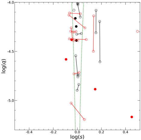
### Visual Description
## Scatter Plot: log(q) vs log(s)
### Overview
The image presents a scatter plot with error bars, displaying the relationship between log(q) and log(s). There are multiple data series represented by different colored markers. A vertical dashed green line is present, potentially indicating a threshold or region of interest.
### Components/Axes
* **X-axis:** log(s), ranging approximately from -0.4 to 0.4. Tick marks are present at -0.4, -0.2, 0, 0.2, and 0.4.
* **Y-axis:** log(q), ranging approximately from -5.0 to -4.0. Tick marks are present at -5.0, -4.5, and -4.0.
* **Data Series 1:** Black circles.
* **Data Series 2:** Red circles.
* **Data Series 3:** Red circles with a surrounding white circle.
* **Error Bars:** Vertical lines extending above and below data points, indicating uncertainty.
* **Vertical Dashed Line:** Green, positioned around log(s) = -0.1.
### Detailed Analysis
Let's analyze each data series and their approximate values.
* **Black Circles:** This series shows a general downward trend.
* (-0.3, -4.2)
* (-0.2, -4.1)
* (-0.1, -4.0)
* (0.0, -4.0)
* (0.1, -4.2)
* **Red Circles:** This series is more scattered.
* (-0.3, -4.4)
* (-0.2, -4.6)
* (-0.1, -4.3)
* (0.0, -4.5)
* (0.1, -4.4)
* (0.2, -4.6)
* (0.3, -4.4)
* (0.4, -4.6)
* **Red Circles with White Surroundings:** This series appears clustered around log(s) = -0.1.
* (-0.3, -4.8)
* (-0.2, -4.7)
* (-0.1, -4.3)
* (0.0, -4.4)
* (0.1, -4.5)
* (0.2, -4.9)
Error bars are present for the red circles with white surroundings, with approximate lengths of +/- 0.2 for most points. The error bars for the other series are not visible.
### Key Observations
* The black circle series exhibits a clear negative correlation between log(q) and log(s).
* The red circle series is more dispersed, with no obvious trend.
* The red circles with white surroundings are concentrated near log(s) = -0.1, and have associated error bars.
* The vertical dashed green line at log(s) = -0.1 may be a point of interest, as the red circles with white surroundings are clustered around it.
### Interpretation
The plot likely represents a relationship between two physical quantities, 'q' and 's', where a logarithmic transformation has been applied to both. The black circle data suggests an inverse relationship – as 's' increases, 'q' decreases. The red circle data may represent noise or a different underlying process. The red circles with white surroundings, clustered around log(s) = -0.1, and with error bars, suggest a specific measurement or condition being investigated. The green dashed line could represent a critical value of 's' or a boundary condition.
Without further context, it's difficult to determine the exact meaning of 'q' and 's'. However, the plot suggests a systematic relationship between them, potentially governed by a power law (given the logarithmic axes). The error bars on the red circles with white surroundings indicate a level of uncertainty associated with those measurements, while the lack of error bars on the other data series suggests either higher precision or that uncertainty is not being considered. The clustering of the red/white data around the green line suggests that this value of 's' is particularly important or relevant to the system being studied.
</details>
in the KMTNet data. Zhu et al. (2014) predicted that ∼ 50% of the KMTNet q < 10 -4 planets should be detected by caustics outside of the near-resonant (Dominik 1999; Yee et al. 2021) range. Below we follow the definitions of Zang et al. (2021b) and refer to caustics inside and outside of the near-resonant range as near-resonant caustics and pureplanetary caustics. Contrary to the prediction of Zhu et al. (2014), before the application of AnomalyFinder only two of ten q < 10 -4 KMTNet planets were detected by pureplanetary caustics. The two cases are OGLE-2017-BLG0173Lb (Hwang et al. 2018a) and KMT-2016-BLG-0212Lb (Hwang et al. 2018b). Hence, it is necessary to check the caustic types for the planetary sample of AnomalyFinder.
Figure 14 shows the log q versus log s plot for the 27 planets. The red and black points represent planets that were first discovered using AnomalyFinder and by-eye searches, respectively. The two green dashed lines indicate the boundaries for the near-resonant range. A striking feature is that in constrast to the locations of the by-eye planets, of the
15 AnomalyFinder planets 11 have pure-planetary caustics, two have both pure-planetary and near-resonant caustics, and only two are fully located inside the near-resonant range. In total, at least 13 planets were detected by pure-planetary caustics. Thus, the caustic types of the AnomalyFinder planetary sample agree with the expectation of Zhu et al. (2014), and the missing planetary caustics problem has been solved by the systematic planetary anomaly search.
## 6.2. Caustic Crossing and Anomaly Type
Zhu et al. (2014) predicted that about half of the KMTNet planets will be detected by caustic-crossing anomalies. Jung et al. (2022) found that 16/33 of 2018 KMTNet AnomalyFinder planets have caustic-crossing anomalies. As shown in Table 14, 14/27 of the q < 10 -4 planets have causticcrossing anomalies, in good agreement with the expectation of Zhu et al. (2014). Thus, the ∼ 50% probability of causticcrossing anomalies is likely applicable down to q ∼ 10 -5 .
Zang et al. (2021b) and Hwang et al. (2022) applied the AnomalyFinder algorithm to 2018-2019 KMTNet primefield events and found seven newly discovered q < 2 × 10 -4 planets. Among them, only OGLE-2019-BLG-1053Lb has a bump-type anomaly and the other six planets were detected by dip-type anomalies. Thus, it is necessary to check whether dip-type anomalies dominate the detection of lowq planets. As presented in Table 14, the ratio of bump-type to dip-type anomalies for the q < 10 -4 planets is 15 to 12, so the two types of anomalies play roughly equal roles in the lowq detection. However, of the 12 dip-type anomalies, nine were solely detected by AnomalyFinder, including eight non-caustic-crossing anomalies. KMT-2018-BLG1988 (Han et al. 2022a) is the only case that the anomaly is a non-caustic-crossing dip and was first discovered from byeye searches. Unlike the dip-type anomalies, the four noncaustic-crossing bumps were all first noticed from by-eye searches. Hence, by-eye searches have proved to be quite insensitive to non-caustic-crossing dip-type anomalies for lowq planets.
## 6.3. A Desert of High-magnification Planetary Signals
Zang et al. (2021b) suggested that the missing planetary caustics problem was caused by the way that modelers searched for planetary signatures. Because highmagnification events are intrinsically more sensitive to planets (Griest & Safizadeh 1998), by-eye searches paid more attention to them, while pure-planetary caustics are mainly detected in low-magnification events. If this hypothesis is correct, we expect that by-eye planets and AnomalyFinder planets will have different | u 0 | and | u anom | distributions. The log | u anom | versus log | u 0 | distribution of Figure 15 confirms our expectation. Except for the two planets that were detected by pure-planetary caustics, all the other by-eye planets, which are located inside the near-resonant range, were
Figure 15. log | u anom | vs. log | u 0 | distribution for the 27 planetary events with q < 10 -4 shown in Table 14. Colors are the same as the colors of Figure 14. Circles and triangles represent prime-field and sub-prime-field planets, respectively. The grey dashed line indicates | u 0 | = | u anom | .
<details>
<summary>Image 15 Details</summary>
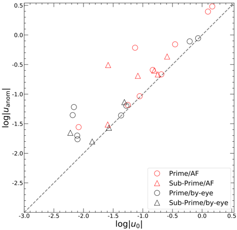
### Visual Description
## Scatter Plot: log(u_anom) vs. log(u_0)
### Overview
This image presents a scatter plot comparing `log(u_anom)` against `log(u_0)` for four different categories of data: Prime/AF, Sub-Prime/AF, Prime/by-eye, and Sub-Prime/by-eye. A dashed line representing the equality line (y=x) is also present. The plot appears to be investigating the relationship between an anomalous velocity component (`u_anom`) and an initial velocity component (`u_0`).
### Components/Axes
* **X-axis:** `log|u_0|` (Logarithm of the absolute value of u_0). Scale ranges from approximately -3.0 to 0.5.
* **Y-axis:** `log|u_anom|` (Logarithm of the absolute value of u_anom). Scale ranges from approximately -2.0 to 0.5.
* **Legend:** Located in the bottom-right corner.
* Prime/AF (Red circles)
* Sub-Prime/AF (Red triangles)
* Prime/by-eye (Black circles)
* Sub-Prime/by-eye (Black triangles)
* **Equality Line:** A dashed grey line with a slope of 1, representing the line where `log|u_anom|` equals `log|u_0|`.
### Detailed Analysis
Let's analyze each data series individually:
* **Prime/AF (Red Circles):** The data points generally cluster above the equality line, indicating that `log|u_anom|` tends to be greater than `log|u_0|`. The trend is roughly linear, with a positive slope. Approximate data points:
* (-2.0, -1.5)
* (-1.5, -0.8)
* (-1.0, -0.3)
* (-0.5, 0.0)
* (0.0, 0.2)
* (0.2, 0.4)
* **Sub-Prime/AF (Red Triangles):** These points also tend to cluster above the equality line, but are more scattered than the Prime/AF data. The trend is also roughly linear, but with more variability. Approximate data points:
* (-2.0, -1.0)
* (-1.5, -0.5)
* (-1.0, -0.2)
* (-0.5, 0.1)
* (0.0, 0.3)
* **Prime/by-eye (Black Circles):** These points are more closely aligned with the equality line than the AF data, but still generally lie above it. The trend is approximately linear. Approximate data points:
* (-2.0, -1.7)
* (-1.5, -1.2)
* (-1.0, -0.7)
* (-0.5, -0.2)
* (0.0, 0.0)
* **Sub-Prime/by-eye (Black Triangles):** These points are the most scattered and show the greatest deviation from the equality line. They are generally below the equality line for lower values of `log|u_0|`, and above it for higher values. Approximate data points:
* (-2.0, -1.8)
* (-1.5, -1.0)
* (-1.0, -0.5)
* (-0.5, 0.0)
* (0.0, 0.2)
### Key Observations
* The "AF" data (both Prime and Sub-Prime) consistently shows `log|u_anom|` greater than `log|u_0|`, suggesting a systematic overestimation of the anomalous velocity component when using the "AF" method.
* The "by-eye" data is closer to the equality line, indicating a more accurate estimation of the anomalous velocity component.
* The Sub-Prime/by-eye data is the most variable, suggesting that the "by-eye" method is less reliable for Sub-Prime data.
* There is a clear distinction between the Prime and Sub-Prime data, particularly when using the "AF" method.
### Interpretation
This plot likely represents a comparison of two methods ("AF" and "by-eye") for estimating an anomalous velocity component (`u_anom`) based on an initial velocity component (`u_0`), separated by loan type (Prime vs. Sub-Prime). The equality line serves as a benchmark for perfect estimation.
The data suggests that the "AF" method systematically overestimates `u_anom` for both Prime and Sub-Prime loans, while the "by-eye" method provides more accurate estimates, particularly for Prime loans. The increased variability in the Sub-Prime/by-eye data suggests that the "by-eye" method is more susceptible to subjective error when applied to Sub-Prime loans.
The difference between the Prime and Sub-Prime data, especially when using the "AF" method, could indicate that the "AF" method is more sensitive to the characteristics of Sub-Prime loans, leading to a greater overestimation of the anomalous velocity component. This could have implications for risk assessment and loan pricing. The plot highlights the importance of carefully considering the method used for estimating `u_anom` and the potential biases associated with each method, particularly when dealing with different loan types.
</details>
detected with | u 0 | 0 . 05 and | u anom | 0 . 07 . The roughly one-dex gap of the by-eye planets, at 0 . 05 | u 0 | 0 . 62 and 0 . 07 | u anom | 0 . 78 , is filled by the AnomalyFinder planets 3 .
However, there is no planet located at the left lower corner of Figure 15, with | u 0 , limit | = 0 . 0060 and | u anom , limit | = 0 . 0158 . Although six of the planets were detected in highmagnification events ( | u 0 | < 0 . 01 ), all the planetary signals occurred on the low- and median-magnification regions. This desert of high-magnification planetary signals could be caused by the insufficient observing cadences of the current KMTNet survey. High-magnification planetary signals for q < 10 -4 events are weak and thus require dense observations over the peak. There are three known q < 10 -4 events whose planetary signals occurred on the high-magnification regions ( | u anom | < 0 . 01 ). They are OGLE-2005-BLG-169 with u anom = 0 . 0012 (Gould et al. 2006), KMT-2021-BLG0171 with | u anom | = 0 . 0066 (Yang et al. 2022), and KMT2022-BLG-0440 with | u anom | = 0 . 0041 (Zhang et al. in
3 Although it might seem that the correlation could be with anomaly brightness rather than | u 0 | (because smaller | u 0 | implies a more highly magnified event), Jung et al. (2022) showed that there is no correlation with event brightness at the time of the anomaly between by-eye vs. AnomalyFinder detections. On the other hand, Hwang et al. (2022) and Zang et al. (2022a) have shown that AnomalyFinder is much better at finding anomalies with smaller ∆ χ 2 .
prep). The follow-up data played decisive roles in these detections and the combined cadences of survey and follow-up data are higher than 30 hr -1 , while the highest cadence of the current KMTNet survey is 8 hr -1 for about 0.4 deg 2 from the overlap of two Γ = 4 hr -1 fields.
However, we note that AnomalyFinder used the KMTNet end-of-year pipeline light curves, for which the photometric quality is not as good as that of TLC re-reductions. For the three follow-up planets, the planetary signals only have ∆ I < 0 . 05 mag. Thus, TLC re-reductions may be needed to recover such weak signals in the KMTNet data, and we cannot rule out the possibility that the desert may also be due to the imperfect KMTNet photometric quality. Each year there are about 20 events with | u 0 | < 0 . 01 observed by KMTNet with Γ ≥ 4 hr -1 . The current KMTNet quasi-automated TLC re-reductions pipeline takes < 1 hr of human effort for each event (H. Yang et al. in prep), so an optimized systematic search for q < 10 -4 planets in the KMTNet highmagnification events can be done very quickly. This search could have important implications for future space-based microlensing projects, because their tentative cadences are similar to or lower than Γ = 4 hr -1 (Penny et al. 2019; Ge et al. 2022; Yan & Zhu 2022). If this search demonstrates that high-magnification events need denser observations to capture the weak planetary signals for lowq planets, one could consider conducting (if feasible) ground-based followup projects for high-magnification events that are discovered by space-based telescopes. We also note that for the 2018 AnomalyFinder planets (Gould et al. 2022; Jung et al. 2022) and 2019 prime-field AnomalyFinder planets (Zang et al. 2022a), which are complete now, only one q > 10 -4 planet, KMT-2019-BLG-1953Lb, has | u anom | < | u anom , limit | . Future analysis of all the 2016-2019 KMTNet should check whether the desert is obvious for more massive planets.
## 6.4. Prime and sub-Prime Fields
In its 2015 commissioning season, KMTNet observed four fields at a cadence of Γ = 6 hr -1 . To support the 2016-2019 Spitzer microlensing campaign (Gould et al. 2013, 2014a, 2015a,b, 2016, 2018) and find more planets, KMTNet monitored a wider area, with a total of (3, 7, 11, 3) fields at cadences of Γ ∼ (4 , 1 , 0 . 4 , 0 . 2) hr -1 . The three fields with the highest cadence are the KMTNet prime fields and the other 21 are the KMTNet sub-prime fields. See Figure 12 of Kim et al. (2018a) for the field placement. As shown in Table 14 and Figure 15, the prime fields played the main role in the detection of q < 10 -4 planets, as predicted by Henderson et al. (2014), and 17 of 27 planets were detected therein. However, the sub-prime fields are also important and six of the ten lowestq planets were discovered therein.
For the six planets with | u 0 | < 0 . 01 , there is a clear bias in cadences, and only one of them was detected from the sub-
prime fields. For the prime and sub-prime fields, the current detection rates are 1.25 and 0.25 per year, respectively. Because ∼ 60% of the KMTNet microlensing events are located in the sub-prime fields, if the sub-prime-field events with | u 0 | < 0 . 01 can had the same cadence as the prime-field events from follow-up observations, each year there would be (1 . 25 × (60% / 40%) -0 . 25) = 1 . 6 more q < 10 -4 planets. Because follow-up observations can have higher cadences and capture the high-magnification planetary signals (e.g., Yang et al. 2022), the yield of a follow-up project can be at least two q < 10 -4 planets per year. The reward is not only enlarging the lowq planetary sample, but also an independent check of the statistical results from AnomalyFinder if the follow-up planets can form a homogeneous statistical sample (Gould et al. 2010). However, this reward requires that the KMTNet alert-finder system should alert new events before they reach the high-magnification regions (e.g., A > 20 ).
We appreciate the anonymous referee for helping to improve the paper. W.Zang, H.Y., S.M., J.Z., and W.Zhu acknowledge support by the National Science Foundation of China (Grant No. 12133005). W.Zang acknowledges the support from the Harvard-Smithsonian Center for Astrophysics through the CfA Fellowship. This research was supported by the Korea Astronomy and Space Science Institute under the R&D program (Project No. 2022-1-830-04) supervised by the Ministry of Science and ICT. This research has made use of the KMTNet system operated by the Korea Astronomy and Space Science Institute (KASI) and the data were obtained at three host sites of CTIO in Chile, SAAO in South Africa, and SSO in Australia. The authors acknowledge the Tsinghua Astrophysics High-Performance Computing platform at Tsinghua University for providing computational and data storage resources that have contributed to the research results reported within this paper. Work by J.C.Y. acknowledges support from N.S.F Grant No. AST2108414. Work by C.H. was supported by the grants of National Research Foundation of Korea (2019R1A2C2085965 and 2020R1A4A2002885). Y.S. acknowledges support from BSF Grant No. 2020740. W.Zhu acknowledges the science research grants from the China Manned Space Project with No. CMS-CSST-2021-A11. This research uses data obtained through the Telescope Access Program (TAP), which has been funded by the TAP member institutes. This research is supported by Tsinghua University Initiative Scientific Research Program (Program ID 2019Z07L02017). This research has made use of the NASA Exoplanet Archive, which is operated by the California Institute of Technology, under contract with the National Aeronautics and Space Administration under the Exoplanet Exploration Program.
## REFERENCES
- Adams, A. D., Boyajian, T. S., & von Braun, K. 2018, MNRAS, 473, 3608, doi: 10.1093/mnras/stx2367
- Bond, I. A., Bennett, D. P., Sumi, T., et al. 2017, MNRAS, 469, 2434, doi: 10.1093/mnras/stx1049
Alard, C., & Lupton, R. H. 1998, ApJ, 503, 325, doi: 10.1086/305984
- Albrow, M. D. 2017, Michaeldalbrow/Pydia: Initial Release On Github., v1.0.0, Zenodo, doi: 10.5281/zenodo.268049
- Albrow, M. D., Horne, K., Bramich, D. M., et al. 2009, MNRAS, 397, 2099, doi: 10.1111/j.1365-2966.2009.15098.x
- An, J. H., Albrow, M. D., Beaulieu, J.-P., et al. 2002, ApJ, 572, 521, doi: 10.1086/340191
- Batista, V., Gould, A., Dieters, S., et al. 2011, A&A, 529, A102, doi: 10.1051/0004-6361/201016111
- Beaulieu, J.-P., Bennett, D. P., Fouqu´ e, P., et al. 2006, Nature, 439, 437, doi: 10.1038/nature04441
- Bennett, D. P., Bond, I. A., Udalski, A., et al. 2008, ApJ, 684, 663, doi: 10.1086/589940
- Bensby, T., Yee, J. C., Feltzing, S., et al. 2013, A&A, 549, A147, doi: 10.1051/0004-6361/201220678
- Bhattacharya, A., Beaulieu, J. P., Bennett, D. P., et al. 2018, AJ, 156, 289, doi: 10.3847/1538-3881/aaed46
- Bond, I. A., Udalski, A., Jaroszy´ nski, M., et al. 2004, ApJL, 606, L155, doi: 10.1086/420928
Bozza, V. 2010, MNRAS, 408, 2188,
- doi: 10.1111/j.1365-2966.2010.17265.x
- Bozza, V., Bachelet, E., Bartoli´ c, F., et al. 2018, MNRAS, 479, 5157, doi: 10.1093/mnras/sty1791
Dominik, M. 1999, A&A, 349, 108
- Dong, S., Gould, A., Udalski, A., et al. 2009, ApJ, 695, 970, doi: 10.1088/0004-637X/695/2/970
- Foreman-Mackey, D., Hogg, D. W., Lang, D., & Goodman, J. 2013, PASP, 125, 306, doi: 10.1086/670067
Gaudi, B. S. 1998, ApJ, 506, 533, doi: 10.1086/306256
- Gaudi, B. S., & Gould, A. 1997, ApJ, 486, 85, doi: 10.1086/304491 Ge, J., Zhang, H., Zang, W., et al. 2022, arXiv e-prints, arXiv:2206.06693. https://arxiv.org/abs/2206.06693
- Gonzalez, O. A., Rejkuba, M., Zoccali, M., et al. 2012, A&A, 543, A13, doi: 10.1051/0004-6361/201219222
- Gould, A. 1992, ApJ, 392, 442, doi: 10.1086/171443
- -. 1996, ApJ, 470, 201, doi: 10.1086/177861
- -. 2000, ApJ, 542, 785, doi: 10.1086/317037
- -. 2004, ApJ, 606, 319, doi: 10.1086/382782
- Gould, A., Carey, S., & Yee, J. 2013, Spitzer Microlens Planets and Parallaxes, Spitzer Proposal
- -. 2014a, Galactic Distribution of Planets from Spitzer Microlens Parallaxes, Spitzer Proposal
- -. 2016, Galactic Distribution of Planets Spitzer Microlens Parallaxes, Spitzer Proposal
- Gould, A., & Loeb, A. 1992, ApJ, 396, 104, doi: 10.1086/171700
- Gould, A., Yee, J., & Carey, S. 2015a, Degeneracy Breaking for K2 Microlens Parallaxes, Spitzer Proposal
- -. 2015b, Galactic Distribution of Planets From High-Magnification Microlensing Events, Spitzer Proposal
- Gould, A., Yee, J., Carey, S., & Shvartzvald, Y. 2018, The Galactic Distribution of Planets via Spitzer Microlensing Parallax, Spitzer Proposal
- Gould, A., Udalski, A., An, D., et al. 2006, ApJL, 644, L37, doi: 10.1086/505421
- Gould, A., Dong, S., Gaudi, B. S., et al. 2010, ApJ, 720, 1073, doi: 10.1088/0004-637X/720/2/1073
- Gould, A., Udalski, A., Shin, I. G., et al. 2014b, Science, 345, 46, doi: 10.1126/science.1251527
- Gould, A., Ryu, Y.-H., Calchi Novati, S., et al. 2020, Journal of Korean Astronomical Society, 53, 9.
https://arxiv.org/abs/1906.11183
- Gould, A., Han, C., Zang, W., et al. 2022, A&A, 664, A13, doi: 10.1051/0004-6361/202243744
- Griest, K., & Safizadeh, N. 1998, ApJ, 500, 37, doi: 10.1086/305729
- Han, C., Udalski, A., Lee, C.-U., et al. 2021, A&A, 649, A90, doi: 10.1051/0004-6361/202039817
- Han, C., Gould, A., Albrow, M. D., et al. 2022a, A&A, 658, A62, doi: 10.1051/0004-6361/202142077
- Han, C., Kim, D., Gould, A., et al. 2022b, A&A, 664, A33, doi: 10.1051/0004-6361/202243484
- Hayashi, C. 1981, in Fundamental Problems in the Theory of Stellar Evolution, ed. D. Sugimoto, D. Q. Lamb, & D. N. Schramm, Vol. 93, 113-126
- Henderson, C. B., Gaudi, B. S., Han, C., et al. 2014, ApJ, 794, 52, doi: 10.1088/0004-637X/794/1/52
- Holtzman, J. A., Watson, A. M., Baum, W. A., et al. 1998, AJ, 115, 1946, doi: 10.1086/300336
- Hwang, K.-H., Choi, J.-Y., Bond, I. A., et al. 2013, ApJ, 778, 55, doi: 10.1088/0004-637X/778/1/55
- Hwang, K.-H., Udalski, A., Shvartzvald, Y., et al. 2018a, AJ, 155, 20, doi: 10.3847/1538-3881/aa992f
- Hwang, K. H., Kim, H. W., Kim, D. J., et al. 2018b, Journal of Korean Astronomical Society, 51, 197, doi: 10.5303/JKAS.2018.51.6.197
- Hwang, K.-H., Zang, W., Gould, A., et al. 2022, AJ, 163, 43, doi: 10.3847/1538-3881/ac38ad
- Ishitani Silva, S., Ranc, C., Bennett, D. P., et al. 2022, AJ, 164, 118, doi: 10.3847/1538-3881/ac82b8
- Jiang, G., DePoy, D. L., Gal-Yam, A., et al. 2004, ApJ, 617, 1307, doi: 10.1086/425678
- Jung, Y. K., Udalski, A., Yee, J. C., et al. 2017, AJ, 153, 129, doi: 10.3847/1538-3881/aa5d07
- Jung, Y. K., Udalski, A., Zang, W., et al. 2020, AJ, 160, 255, doi: 10.3847/1538-3881/abbe93
- Jung, Y. K., Zang, W., Han, C., et al. 2022, AJ, 164, 262, doi: 10.3847/1538-3881/ac9c5c
- Kennedy, G. M., & Kenyon, S. J. 2008, ApJ, 673, 502, doi: 10.1086/524130
- Kim, D.-J., Kim, H.-W., Hwang, K.-H., et al. 2018a, AJ, 155, 76, doi: 10.3847/1538-3881/aaa47b
- Kim, H.-W., Hwang, K.-H., Shvartzvald, Y., et al. 2018b, arXiv e-prints, arXiv:1806.07545. https://arxiv.org/abs/1806.07545
- Kim, S.-L., Lee, C.-U., Park, B.-G., et al. 2016, Journal of Korean Astronomical Society, 49, 37, doi: 10.5303/JKAS.2016.49.1.037
- Kondo, I., Yee, J. C., Bennett, D. P., et al. 2021, AJ, 162, 77, doi: 10.3847/1538-3881/ac00ba
- Mao, S., & Paczynski, B. 1991, ApJL, 374, L37, doi: 10.1086/186066
- Min, M., Dullemond, C. P., Kama, M., & Dominik, C. 2011, Icarus, 212, 416, doi: 10.1016/j.icarus.2010.12.002
- Muraki, Y., Han, C., Bennett, D. P., et al. 2011, ApJ, 741, 22, doi: 10.1088/0004-637X/741/1/22
- Nataf, D. M., Gould, A., Fouqu´ e, P., et al. 2013, ApJ, 769, 88, doi: 10.1088/0004-637X/769/2/88
- Nataf, D. M., Gonzalez, O. A., Casagrande, L., et al. 2016, MNRAS, 456, 2692, doi: 10.1093/mnras/stv2843
- Paczy´ nski, B. 1986, ApJ, 304, 1, doi: 10.1086/164140
- Penny, M. T., Gaudi, B. S., Kerins, E., et al. 2019, ApJS, 241, 3, doi: 10.3847/1538-4365/aafb69
- Poindexter, S., Afonso, C., Bennett, D. P., et al. 2005, ApJ, 633, 914, doi: 10.1086/468182
- Ranc, C., Bennett, D. P., Hirao, Y., et al. 2019, AJ, 157, 232, doi: 10.3847/1538-3881/ab141b
- Rota, P., Hirao, Y., Bozza, V., et al. 2021, AJ, 162, 59, doi: 10.3847/1538-3881/ac0155
- Ryu, Y.-H., Udalski, A., Yee, J. C., et al. 2020, AJ, 160, 183, doi: 10.3847/1538-3881/abaa3f
- Ryu, Y.-H., Kil Jung, Y., Yang, H., et al. 2022, AJ, 164, 180, doi: 10.3847/1538-3881/ac8d6c
- Sako, T., Sekiguchi, T., Sasaki, M., et al. 2008, Experimental Astronomy, 22, 51, doi: 10.1007/s10686-007-9082-5
- Shvartzvald, Y., Yee, J. C., Calchi Novati, S., et al. 2017, ApJL, 840, L3, doi: 10.3847/2041-8213/aa6d09
- Skowron, J., Udalski, A., Gould, A., et al. 2011, ApJ, 738, 87, doi: 10.1088/0004-637X/738/1/87
- Sumi, T., Bennett, D. P., Bond, I. A., et al. 2010, ApJ, 710, 1641, doi: 10.1088/0004-637X/710/2/1641
- Suzuki, D., Bennett, D. P., Sumi, T., et al. 2016, ApJ, 833, 145, doi: 10.3847/1538-4357/833/2/145
- Szyma´ nski, M. K., Udalski, A., Soszy´ nski, I., et al. 2011, AcA, 61, 83. https://arxiv.org/abs/1107.4008
- Tomaney, A. B., & Crotts, A. P. S. 1996, AJ, 112, 2872, doi: 10.1086/118228
- Udalski, A. 2003, AcA, 53, 291
Udalski, A., Szymanski, M., Kaluzny, J., et al. 1994, AcA, 44, 227
- Udalski, A., Szyma´ nski, M. K., & Szyma´ nski, G. 2015, AcA, 65, 1. https://arxiv.org/abs/1504.05966
- Udalski, A., Ryu, Y.-H., Sajadian, S., et al. 2018, AcA, 68, 1. https://arxiv.org/abs/1802.02582
- Wang, H., Zang, W., Zhu, W., et al. 2022, MNRAS, 510, 1778, doi: 10.1093/mnras/stab3581
- Wang, T., Calchi Novati, S., Udalski, A., et al. 2018, ApJ, 860, 25, doi: 10.3847/1538-4357/aabcd2
- Wozniak, P. R. 2000, AcA, 50, 421
- Yan, S., & Zhu, W. 2022, Research in Astronomy and Astrophysics, 22, 025006, doi: 10.1088/1674-4527/ac3c44
- Yang, H., Zang, W., Gould, A., et al. 2022, MNRAS, 516, 1894, doi: 10.1093/mnras/stac2023
- Yee, J. C., Zang, W., Udalski, A., et al. 2021, AJ, 162, 180, doi: 10.3847/1538-3881/ac1582
- Yoo, J., DePoy, D. L., Gal-Yam, A., et al. 2004, ApJ, 603, 139, doi: 10.1086/381241
- Zang, W., Han, C., Kondo, I., et al. 2021a, Research in Astronomy and Astrophysics, 21, 239, doi: 10.1088/1674-4527/21/9/239
- Zang, W., Hwang, K.-H., Udalski, A., et al. 2021b, AJ, 162, 163, doi: 10.3847/1538-3881/ac12d4
- Zang, W., Yang, H., Han, C., et al. 2022a, MNRAS, 515, 928, doi: 10.1093/mnras/stac1883
- Zang, W., Shvartzvald, Y., Udalski, A., et al. 2022b, MNRAS, 514, 5952, doi: 10.1093/mnras/stac1631
- Zhang, K., & Gaudi, B. S. 2022, ApJL, 936, L22, doi: 10.3847/2041-8213/ac8c2b
- Zhang, K., Gaudi, B. S., & Bloom, J. S. 2022, Nature Astronomy, 6, 782, doi: 10.1038/s41550-022-01671-6
- Zhu, W., Penny, M., Mao, S., Gould, A., & Gendron, R. 2014, ApJ, 788, 73, doi: 10.1088/0004-637X/788/1/73
- Zhu, W., Udalski, A., Calchi Novati, S., et al. 2017, AJ, 154, 210, doi: 10.3847/1538-3881/aa8ef1
Table 14 . Information of 2016-2019 KMTNet AnomalyFinder planetary sample with q < 10 -4 solutions
| Event Name | KMTNet Name | log q | s | | u 0 | | Method | ∆ χ 2 | Caustic-Crossing | Anomaly Type | Field |
|--------------|---------------|------------------------------|-------------------|---------------------|-----------|---------|--------------------|----------------|-----------|
| KB161105 1 | KB161105 | - 5 . 194 ± 0 . 248 | 1 . 143 ± 0 . 009 | 0.171 | Discovery | 0.0 | yes | bump | sub-prime |
| | | - 4 . 423 ± 0 . 197 | 1 . 136 ± 0 . 011 | 0.153 | | 2.3 | yes | | |
| | | - 4 . 184 ± 0 . 206 | 1 . 106 ± 0 . 013 | 0.154 | | 2.7 | no | | |
| | | - 5 . 027 ± 0 . 080 | 0 . 888 ± 0 . 007 | 0.148 | | 3.5 | no | | |
| | | - 4 . 069 ± 0 . 182 | 0 . 892 ± 0 . 005 | 0.154 | | 4.4 | yes | | |
| OB160007 2 | KB161991 | - 5 . 168 ± 0 . 131 | 2 . 829 ± 0 . 009 | 1.253 | Discovery | | yes | bump | prime |
| OB191053 3 | KB191504 | - 4 . 885 ± 0 . 035 | 1 . 406 ± 0 . 011 | 0.373 | Discovery | | yes | bump | prime |
| OB190960 4 | KB191591 | - 4 . 830 ± 0 . 041 | 1 . 029 ± 0 . 001 | 0.0061 | Recovery | 0.0 | yes | bump | sub-prime |
| | | - 4 . 896 ± 0 . 024 | 0 . 997 ± 0 . 001 | 0.0060 | | 1.0 | yes | | |
| | | - 4 . 896 ± 0 . 024 | 0 . 996 ± 0 . 001 | 0.0059 | | 1.9 | yes | | |
| | | - 4 . 845 ± 0 . 043 | 1 . 028 ± 0 . 001 | 0.0061 | | 2.1 | yes | | |
| KB180029 5 | KB180029 | - 4 . 737 ± 0 . 047 | 0 . 999 ± 0 . 002 | 0.027 | Recovery | 0.0 | yes | bump | sub-prime |
| | | - 4 . 746 ± 0 . 050 | 1 . 028 ± 0 . 002 | 0.027 | | 0.2 | yes | | |
| | | - 4 . 740 ± 0 . 045 | 0 . 999 ± 0 . 002 | 0.027 | | 2.1 | yes | | |
| | | - 4 . 736 ± 0 . 050 | 1 . 028 ± 0 . 002 | 0.027 | | 2.2 | yes | | |
| KB191806 1 | KB191806 | - 4 . 714 ± 0 . 116 | 1 . 035 ± 0 . 009 | 0.0255 | Discovery | 0.0 | no | dip | sub-prime |
| | | - 4 . 717 ± 0 . 117 | 1 . 034 ± 0 . 009 | 0.0257 | | 0.4 | no | | |
| | | - 4 . 724 ± 0 . 117 | 0 . 938 ± 0 . 007 | 0.0260 | | 0.7 | no | | |
| | | - 4 . 734 ± 0 . 109 | 0 . 938 ± 0 . 007 | 0.0251 | | 1.1 | no | | |
| OB170173 6 | KB171707 | - 4 . 606 ± 0 . 042 | 1 . 540 ± 0 . 031 | 0.867 | Recovery | 0.0 | yes | bump | prime |
| | | - 4 . 195 ± 0 . 068 | 1 . 532 ± 0 . 025 | 0.844 | | 3.5 | yes | | |
| KB171194 1 | KB171194 | - 4 . 582 ± 0 . 058 | 0 . 806 ± 0 . 010 | 0.256 | Discovery | | no | dip | sub-prime |
| | | - 4 . 759 +0 . 698 - 0 . 618 | | | | | | | |
| | | - 0 . 168 | 1 . 01 ± 0 . 05 | 0.014 | | 0.1 | no | | |
| KB190842 8 | KB190842 | - 4 . 389 ± 0 . 031 | 0 . 983 ± 0 . 013 | 0.0066 | Recovery | | no | bump | prime |
| KB190253 9 | KB190253 | - 4 . 387 ± 0 . 076 | 1 . 009 ± 0 . 009 | 0.0559 | Discovery | 0.0 | no | dip | prime |
| | | - 4 . 390 ± 0 . 080 | 0 . 929 ± 0 . 007 | 0.0555 | | 0.3 | no | | |
| OB180977 9 | KB180728 | - 4 . 382 ± 0 . 045 | 0 . 897 ± 0 . 007 | 0.147 | Discovery | | yes | dip | prime |
| KB171003 1 | KB171003 | - 4 . 373 ± 0 . 144 | 0 . 910 ± 0 . 005 | 0.179 | Discovery | 0.0 | no | dip | sub-prime |
| | | - 4 . 260 ± 0 . 152 | 0 . 889 ± 0 . 004 | 0.179 | | 0.2 | no | | |
| OB171806 1 | KB171021 | - 4 . 352 ± 0 . 171 | 0 . 857 ± 0 . 008 | 0.026 | Discovery | 0.0 | yes | bump | sub-prime |
| | | - 4 . 392 ± 0 . 180 | 0 . 861 ± 0 . 007 | 0.025 | | 0.2 | yes | | |
| | | - 4 . 441 ± 0 . 168 | 1 . 181 ± 0 . 011 | 0.026 | | 8.3 | yes | | |
| | | - 4 . 317 ± 0 . 126 | 1 . 190 ± 0 . 012 | 0.027 | | 8.4 | yes | | |
| OB161195 10 | KB160372 | - 4 . 325 ± 0 . 037 | 0 . 989 ± 0 . 004 | 0.0526 | Recovery | 0.0 | no | bump | prime |
| | | - 4 . 318 ± 0 . 038 | 1 . 079 ± 0 . 004 | 0.0526 | | 0.1 | no | | |
| OB170448 2 | KB170090 | - 4 . 296 ± 0 . 149 | 3 . 157 ± 0 . 022 | 1.482 | Discovery | | yes | bump | prime |
| | | - 2 . 705 ± 0 . 045 | 0 . 431 ± 0 . 004 | 1.486 | | 5.8 | yes | | |
| | | - 3 . 969 ± 0 . 086 | 3 . 593 ± 0 . 045 | 1.611 | | 9.7 | yes | | |
| KB191367 1 | KB191367 | - 4 . 303 ± 0 . 118 | 0 . 939 ± 0 . 007 | 0.083 | Discovery | 0.0 | no | dip | sub-prime |
| | | - 4 . 298 ± 0 . 103 | 0 . 976 ± 0 . 007 | 0.082 | | 0.2 | no | | |
| KB170428 1 | KB170428 | - 4 . 295 ± 0 . 072 | 0 . 882 ± 0 . 004 | 0.205 | Discovery | 0.0 | no | dip | prime |
| | | - 4 . 302 ± 0 . 075 | 0 . 915 ± 0 . 005 | 0.205 | | 0.1 | no | | |
| OB171434 11 | KB170016 | - 4 . 242 ± 0 . 011 | 0 . 979 ± 0 . 001 | 0.043 | Recovery | 0.0 | yes | dip | prime |
| | | - 4 . 251 ± 0 . 012 | 0 . 979 ± 0 . 001 | 0.043 | | 4.0 | yes | | |
| OB181185 12 | KB181024 | - 4 . 163 ± 0 . 014 | 0 . 963 ± 0 . 001 | 0.0069 | Recovery | | no | bump | prime |
| OB181126 13 | KB182064 | - 4 . 130 ± 0 . 280 | 0 . 852 ± 0 . 040 | 0.0083 | Discovery | 0.0 | no | dip | prime |
|---------------|------------|-----------------------|---------------------|----------|-------------|-------|------|-------|-----------|
| | | - 4 . 260 ± 0 . 290 | 1 . 154 ± 0 . 052 | 0.0082 | | 2.1 | no | | |
| OB180506 9 | KB180835 | - 4 . 117 ± 0 . 133 | 1 . 059 ± 0 . 021 | 0.0884 | Discovery | 0 | no | dip | prime |
| | | - 4 . 109 ± 0 . 126 | 0 . 861 ± 0 . 018 | 0.0884 | | 0.4 | no | | |
| KB181025 14 | KB181025 | - 4 . 081 ± 0 . 141 | 0 . 937 ± 0 . 021 | 0.0071 | Recovery | 0 | no | bump | prime |
| | | - 3 . 789 ± 0 . 133 | 0 . 883 ± 0 . 025 | 0.0086 | | 8.4 | no | | |
| OB171691 15 | KB170752 | - 4 . 013 ± 0 . 152 | 1 . 003 ± 0 . 014 | 0.0495 | Recovery | 0 | yes | bump | sub-prime |
| | | - 4 . 150 ± 0 . 141 | 1 . 058 ± 0 . 011 | 0.0483 | | 0.4 | yes | | |
| OB180532 16 | KB181161 | - 4 . 011 ± 0 . 053 | 1 . 013 ± 0 . 001 | 0.0082 | Recovery | 0 | yes | dip | prime |
| | | - 4 . 033 ± 0 . 047 | 1 . 011 ± 0 . 001 | 0.0071 | | 2 | yes | | |
| | | - 3 . 926 ± 0 . 049 | 1 . 013 ± 0 . 001 | 0.0089 | | 4.6 | yes | | |
| | | - 4 . 016 ± 0 . 076 | 1 . 011 ± 0 . 001 | 0.0074 | | 5.4 | yes | | |
| KB160625 2 | KB160625 | - 3 . 628 ± 0 . 226 | 0 . 741 ± 0 . 009 | 0.073 | Discovery | 0 | yes | bump | prime |
| | | - 4 . 138 ± 0 . 159 | 1 . 367 ± 0 . 018 | 0.075 | | 1 | yes | | |
| | | - 3 . 746 ± 0 . 291 | 0 . 741 ± 0 . 009 | 0.072 | | 1 | yes | | |
| | | - 4 . 499 ± 0 . 266 | 1 . 358 ± 0 . 015 | 0.076 | | 3.3 | yes | | |
| KB160212 17 | KB160212 | - 1 . 434 ± 0 . 072 | 0 . 829 ± 0 . 007 | 0.328 | Recovery | 0 | yes | bump | prime |
| | | - 4 . 310 ± 0 . 070 | 1 . 427 ± 0 . 014 | 0.615 | | 6.6 | yes | | |
| | | - 4 . 315 ± 0 . 099 | 1 . 434 ± 0 . 012 | 0.619 | | 8 | yes | | |
| | | - 4 . 082 ± 0 . 080 | 1 . 430 ± 0 . 015 | 0.617 | | 8.7 | yes | | |
NOTE: For each planet, we only consider the models that have ∆ χ 2 < 10 compared to the best-fit model. 'Discovery' represents that the planet was discovered using AnomlyFinder, and 'Recovery' means that the planet was first discovered from by-eye searches and then recovered by AnomlyFinder.
Reference: 1. This work; 2. in prep; 3. Zang et al. (2021b); 4. Yee et al. (2021); 5. Gould et al. (2020), Zhang et al. in prep;
6. Hwang et al. (2018a); 7. Han et al. (2022a); 8. Jung et al. (2020); 9. Hwang et al. (2022); 10. Shvartzvald et al. (2017), Bond et al. (2017), Zhang et al. in prep; 11. Udalski et al. (2018); 12. Kondo et al. (2021); 13. Gould et al. (2022); 14. Han et al. (2021); 15. Han et al. (2022b); 16. Ryu et al. (2020); 17. Hwang et al. (2018b).