# Inferring Past Human Actions in Homes with Abductive Reasoning
Abstract
Abductive reasoning aims to make the most likely inference for a given set of incomplete observations. In this paper, we introduce “Abductive Past Action Inference", a novel research task aimed at identifying the past actions performed by individuals within homes to reach specific states captured in a single image, using abductive inference. The research explores three key abductive inference problems: past action set prediction, past action sequence prediction, and abductive past action verification. We introduce several models tailored for abductive past action inference, including a relational graph neural network, a relational bilinear pooling model, and a relational transformer model. Notably, the newly proposed object-relational bilinear graph encoder-decoder (BiGED) model emerges as the most effective among all methods evaluated, demonstrating good proficiency in handling the intricacies of the Action Genome dataset. The contributions of this research significantly advance the ability of deep learning models to reason about current scene evidence and make highly plausible inferences about past human actions. This advancement enables a deeper understanding of events and behaviors, which can enhance decision-making and improve system capabilities across various real-world applications such as Human-Robot Interaction and Elderly Care and Health Monitoring. Code and data available at https://github.com/LUNAProject22/AAR
1 Introduction
Reasoning is an inherent part of human intelligence as it allows us to draw conclusions and construct explanations from existing knowledge when dealing with an uncertain scenario. One of the reasoning abilities that humans possess is abductive reasoning. Abductive reasoning aims to infer the most compelling explanation for a given set of observed facts based on a logical theory. In this work, we study the new problem of inferring past human actions from visual information using abductive inference. It is an extremely useful tool in our daily life, as we often rely on a set of facts to form the most probable conclusion. In fact, a comprehensive understanding of a situation requires considering both past and future information. The ability to perform abductive reasoning about past human actions is vital for human-robot collaboration AI-assisted accident and crime investigation and assistive robotics. Furthermore, robots working in dynamic environments benefit from understanding previous human actions to better anticipate future behaviour or adapt their actions accordingly. Imagine the scenario where a rescue robot enters an elderly person’s house to check on why he or she is not responding to the routine automated phone call. Upon entering the house, the robot observes its surroundings and notices that the back door is left open but nothing else is out of the ordinary. These observations may form a basis for a rational agent – the elderly might have opened the door and went into the garden. The robot can immediately make its way to search for him/her in the back garden. This example illustrates how a social rescue robot can utilize observed facts from the scene to infer past human actions, thereby reasoning about the individual’s whereabouts and ensuring their safety through abductive reasoning.
In recent years, there have been some great initiatives made in abductive reasoning for computer vision [25, 48, 19]. In particular, [25] generates the description of the hypothesis and the premises in the natural language given a video snapshot of events. Without the generation of a hypothesis description, these methods boil down to dense video captioning. A similar task is also presented in [19] where given an image, the model must perform logical abduction to explain the observation in natural language. The use of natural language queries in these tasks presents challenges related to language understanding, making the abductive reasoning task more complicated.
In contrast to these recent works, we challenge a model to infer multiple human actions that may have occurred in the past from a given image. Based on the visual information from the image, objects such as a person, glass and cabinet, may provide clues from which humans can draw conclusions – see Fig. 1. We term this new task, Abductive Past Action Inference and further benchmark how deep learning models perform on this challenging new task. For this task, the models are not only required to decipher the effects of human actions resulting in different environment states but also solve causal chains of action effects, a task that can be challenging even for humans. Furthermore, the task relies on the model’s ability to perform abductive reasoning based on factual evidence i.e., determining what actions may have or have not been performed based on visual information in the image. Humans can solve this task by using prior experience (knowledge) about actions and their effects and using reasoning to make logical inferences. Are deep learning models able to perform abductive past action inference by utilizing visual knowledge present in a given image and a learned understanding of the domain? We aim to answer this question in this paper.
Human action can be viewed as an evolution of human-object relationships over time. Therefore, the state of human-object relations in a scene may give away some cues about the actions that may have been executed by the human. We hypothesize that deep learning models are able to perform logical abduction on past actions using visual and semantic information of human-object relations in the scene. As these human-object relations provide substantial visual cues about actions and the effects of past actions, it makes it easier for the models to infer past actions. On the other hand, there is also the duality in which the evidence should support those conclusions (the actions inferred by the model). If a human executed a set of actions $\mathcal{A}$ which resulted in a state whereby a human-object relation set $\mathcal{R}$ is formed as an effect of those executed actions (i.e., $\mathcal{A}→\mathcal{R}$ ), then using the relational information, we can formulate the task by aiming to infer $\mathcal{A}$ from $\mathcal{R}$ . Therefore, we argue that human-object relational representations are vital for abductive past action inference and provide further justifications in our experiments.
In this work, our models rely on the human-centric object relation tuples such as (person, glass) and (person, closet) obtainable from a single image at the current point in time to perform abductive past action inference. One can see why these human-centric relations are vital for identifying past actions: the (person, glass) relation may lead to deriving actions such as (person-pouring-water, person-took-glass-from-somewhere) while (person, closet) may imply actions such as (person-opening-closet, person-closing-closet) see – Figure 1. Therefore, we use objects and their relationships in the scene to construct human-centric object relations within each image. These relations are made up of both visual and semantic features of recognized objects. To effectively model relational information, we use bilinear pooling and to model inter-relational reasoning, we use a new relational graph neural network (GNN). We propose a new model called BiGED that uses both bilinear pooling and GNNs to effectively reason over human-object relations and inter-relational information of an image to perform abductive inference on past actions effectively.
Our contributions are summarized as follows: (1) To the best of our knowledge, we are the first to propose the abductive past action inference task, which involves predicting past actions through abductive inference. (2) We benchmark several image, video, vision-language, and object-relational models on this problem, thereby illustrating the importance of human-object relational representations. Additionally, we develop a new relational rule-based inference model which serve as relevant baseline models for the abductive past action inference task. (3) We propose a novel relational bilinear graph dncoder-decoder model (BiGED) to tackle this challenging reasoning problem and show the effectiveness of this new design.
2 Related Work
Our work is different from action recognition [20, 18] in a fundamental way. First, in action recognition, the objective is to identify the actions executed in the visible data (e.g., a video or an image in still image action recognition [15]). In action recognition, the models can learn from visual cues what the action looks like and what constitutes an action. In our work, we aim to infer past actions that the model has never seen the human performing. The model only sees visual evidence (e.g. human-object relations) in the scene which is the outcome of executed actions. There are no motion cues or visual patterns of actions that the model can rely on to predict past actions. From a single static image, the machine should infer what actions may have been executed. This is drastically different from classical action recognition and action anticipation tasks.
Abductive past action inference shares some similarity to short-term action anticipation [11, 9] and long-term action anticipation [1]. However, there are several notable differences between the two tasks. Firstly, in abductive past action inference, the goal of the model is to identify the most plausible actions executed by a human in the past based on the current evidence, whereas, in action anticipation, the model learns to predict future action sequences from current observations. The primary distinction lies in abductive past action inference, where observations (evidence) may imply certain past actions, contrasting with action anticipation tasks that predict future actions without certainty. In other words, in abductive past action inference, the evidence and clues indicate possible actions executed in the past that resulted in the evidence or clues. However, in action anticipation, the clues [37], context [14], current actions [13], and knowledge about the task [49] are used to infer probable future actions, but there is no guarantee that the predicted actions will be executed by a human. For instance, observing a person cleaning a room with a broom suggests prior actions such as picking up the broom from somewhere must have happened among many others. Even if putting away the broom is anticipated somewhere in the future, other actions such as holding the broom and opening a window are also possible. Therefore, while action anticipation addresses the uncertainty of future human behavior, abductive past action inference models can utilize scene evidence (such as objects in the scene) to infer the most likely past actions. Additionally, in abductive past action inference, the uncertainty arises from the fact that several different actions may have resulted in similar states $\mathcal{R}$ . In our task, models should comprehend the consequences of each executed action and engage in abductive reasoning to infer the most probable set or sequence of past actions. Another key difference between action anticipation and abductive past action inference is that in action anticipation, predictions made at time $t$ can leverage all past observations. In contrast, abductive past action inference relies solely on present and future information, where new future observations can potentially alter the evidence about past actions, making the inference process more challenging.
Visual Commonsense Reasoning (VCR) [47, 45] and causal video understanding [30, 31] are also related to our work. In VCR [47], given an image, object regions, and a question, the model should answer the question regarding what is happening in the given frame. The model has to also provide justifications for the selected answer in relation to the question. Authors in [29] also studied a similar problem where a dynamic story underlying the input image is generated using commonsense reasoning. In particular, VisualCOMET [29] extends VCR and attempts to generate a set of textual descriptions of events at present, a set of commonsense inferences on events before, a set of commonsense inferences on events after, and a set of commonsense inferences on people’s intents at present. In this vein, given the complete visual commonsense graph representing an image, they propose two tasks; (1) generate the rest of the visual commonsense graph that is connected to the current event and (2) generate a complete set of commonsense inferences. In contrast, given an image without any other natural language queries, we recognize visual objects in the scene and how they are related to the human, then use the human-centric object relational representation to infer the most likely actions executed by the human.
Recently, there are machine learning models that can also perform logical reasoning [6, 50, 4, 16, 22]. Visual scene graph generation [42] and spatial-temporal scene graph generation [5] are also related to our work. Graph neural networks are also related to our work [39, 46, 40]. Our work is also related to bilinear pooling methods such as [12, 10].
<details>
<summary>extracted/6142422/images/tasks_without.png Details</summary>
### Visual Description
## Diagram: Abductive Action Inference
### Overview
The image presents a diagram illustrating a process called "Abductive Action Inference," broken down into three stages: Object Detection, Relational Modelling, and Abductive Action Inference. The Abductive Action Inference stage is further divided into three steps: Set of actions, Sequence of actions, and Language query-based action verification. Each stage is visually represented with images and text descriptions.
### Components/Axes
* **Header:** The title "Abductive Action Inference" is at the top-right, spanning the last third of the diagram.
* **Stage 1: Object Detection:** Located on the left, with a gray arrow pointing to the right. It contains an image of a person holding a bottle and a glass, with bounding boxes around the bottle (cyan), the glass (red), and the person (green).
* **Stage 2: Relational Modelling:** Located in the middle, with a purple arrow pointing to the right. It contains two images: one showing a bottle pouring liquid (cyan bounding box) and another showing a glass being held (red bounding box), with bounding boxes around the person (green). A green arrow indicates the flow from the bottle to the glass.
* **Stage 3: Abductive Action Inference:** Located on the right, divided into three steps.
* **Step 1: Set of actions:** Lists possible actions.
* **Step 2: Sequence of actions:** Lists a sequence of actions.
* **Step 3: Language query-based action verification:** Lists questions and their corresponding "Yes" or "No" answers.
### Detailed Analysis
**Object Detection:**
* Image: A person is holding a white bottle (cyan bounding box) and pouring liquid into a glass (red bounding box). The person is enclosed in a green bounding box.
**Relational Modelling:**
* Image 1: A white bottle (cyan bounding box) is pouring liquid.
* Image 2: A glass (red bounding box) is being held. The person is enclosed in a green bounding box.
* A green arrow indicates the action of pouring from the bottle into the glass.
**Abductive Action Inference:**
* **Step 1: Set of actions:**
* Take glass
* Hold glass
* Open cabinet
* Close cabinet
* Pour into glass
* **Step 2: Sequence of actions:**
1. Open cabinet
2. Take glass
3. Close cabinet
4. Hold glass
5. Pour into glass
* **Step 3: Language query-based action verification:**
* Open cabinet? Yes. (Green)
* Take glass? Yes. (Green)
* Close cabinet? Yes. (Green)
* Hold glass? Yes. (Green)
* Pour into glass? Yes. (Green)
* Drinking? No. (Red)
* Washing glass? No. (Red)
### Key Observations
* The diagram illustrates a pipeline for understanding actions in a scene.
* Object Detection identifies objects in the scene.
* Relational Modelling establishes relationships between the objects.
* Abductive Action Inference uses the identified objects and relationships to infer the actions being performed.
* The Language query-based action verification step uses questions to confirm the inferred actions.
### Interpretation
The diagram presents a system for automated action recognition. It starts with identifying objects in a scene (Object Detection), then models the relationships between these objects (Relational Modelling), and finally infers the actions being performed based on the objects and their relationships (Abductive Action Inference). The language-based verification step adds a layer of confirmation, likely using natural language processing to validate the inferred actions. The "Yes" and "No" answers suggest a binary classification approach for action verification. The negative responses to "Drinking?" and "Washing glass?" indicate the system can differentiate between similar actions based on context.
</details>
Figure 1: Proposed object-relational approach for abductive past action inference. Models are tasked to: 1) abduct the set of past actions, 2) abduct the sequence of past actions, and 3) perform abductive past action verification.
3 Abductive Past Action Inference
Task: Given a single image, models have to infer past actions executed by humans up to the current moment in time. We name this task Abductive Past Action Inference. Let us denote a human action by $a_{i}∈ A$ where $A$ is the set of all actions and $E_{1},E_{2},·s$ is a collection of evidence from the evidence set $\mathcal{E}$ . As the evidence is a result of actions, we can write the logical implication $\mathcal{A}→\mathcal{E}$ where $\mathcal{A}$ is the set of actions executed by a human which resulted in a set of evidence $\mathcal{E}$ . Then, the task aims to derive 1) the set of past actions, 2) the sequence of past actions that resulted in the current evidence shown in the image, and 3) abductive past action verification. The abductive past action verification is a binary task where the model is given a single image and is required to answer a yes or no to an action query (did the person execute action $a_{x}$ in the past?).
3.1 Object-Relational Representation Approach
Our primary hypothesis is that human-object relations are essential for abductive past action inference. Therefore, we propose a human-object relational approach for the task. In all three tasks, our general approach is as follows. We make use of detected humans and objects in the image and then generate a representation for human-centric object relations. Then, using these human-centric object relations, we summarize the visual image, and using neural models, we infer the most likely actions executed by the human. The overview of this approach is shown in Figure 1. Next, we first discuss abductive past action set inference, followed by the details of abductive past action verification.
Abductive past action set prediction.
Let us denote the object by $o∈ O$ , the predicate category by $p∈ P$ , and the human by $h$ . The $j^{th}$ relation $R_{j}$ is a triplet of the form $\left<h,p,o\right>$ . In the $i^{th}$ image, we observe $n$ number of relations $\mathcal{R}_{i}=\{R_{1},R_{2},·s R_{n}\}$ where $\mathcal{R}_{i}$ is the relation set present in the situation shown in that image. These relations constitute the evidence ( $\mathcal{E}$ ). The relation set $\mathcal{R}_{i}$ is an effect of a person executing an action set/sequence $\mathcal{A}_{i}=\{a_{1},·s a_{K}\}$ . Therefore, the following association holds.
$$
\mathcal{A}_{i}\rightarrow\mathcal{R}_{i} \tag{1}
$$
However, we do not know which action caused which relation (evidence), as this information is not available. The association reveals that there is a lack of specific knowledge about the exact effects of individual actions and when multiple actions have been executed, the resulting effect is a combined effect of all executed actions. Consequently, the learning mechanism must uncover the probable cause-and-effect relationships concerning actions. Therefore, given $\mathcal{R}$ we aim to perform abductive past action inference to infer the most likely set of actions executed by the human using neural network learning.
We learn this abduction using the deep neural network functions $\phi()$ , and $\phi_{c}()$ . The relational model, $\phi$ takes relation set as input and outputs a summary of relational information as a vector $x_{r}$ .
$$
x_{r}=\phi(R_{1},\cdots,R_{n};\theta_{\phi}) \tag{2}
$$
The parameters of the relational model are denoted by $\theta_{\phi}$ . The linear classifier ( $\phi_{c}$ ) having the parameters $\theta_{{c}}$ , takes relational information as a vector $x_{r}$ as input and returns the conditional probability of actions given the relational evidence as follows:
$$
P(a_{1},\cdots,a_{K}|R_{1},\cdots,R_{n})=\phi_{c}(x_{r};\theta_{{c}}) \tag{3}
$$
The training and inference sets comprise images and corresponding action set $\mathcal{A}_{i}$ . From each image, we extract the relation set $\mathcal{R}_{i}$ . Therefore, the dataset consists of $\mathcal{D}=\bigcup_{i}\{\mathcal{R}_{i},\mathcal{A}_{i}\}$ . Given the training set ( $\mathcal{D}$ ), we learn the model function in Equations 2 and 3 using backpropagation as follows:
$$
\theta_{\phi}^{*},\theta_{{c}}^{*}=\texttt{argmin}_{\theta_{\phi},\theta_{{c}}%
}\sum_{i}-log(P(\mathcal{A}_{i}|\mathcal{R}_{i})) \tag{4}
$$
where $\theta_{\phi}^{*},\theta_{{c}}^{*}$ are the optimal parameters. As this is a multi-label-multi-class classification problem, we utilize the max-margin multi-label loss from PyTorch where the margin is set to 1, during training.
Abductive past action verification.
Abductive verification model $\phi_{ver}()$ takes the evidence $\mathcal{E}$ and the semantic representation of the past action (e.g. textual encoding of the action name) $y_{a}$ as inputs and outputs a binary classification score indicating if the evidence supports the action or not, i.e. $\phi_{ver}(\mathcal{E},y_{a})→[0,1]$ . Specifically, we encode the past action name using the CLIP [33] text encoder to obtain the textual encoding $y_{a}$ for action class $a$ . Then, we concatenate $y_{a}$ with $x_{r}$ and utilize a two-layer MLP to perform binary classification to determine whether action $a$ was executed or not. We use the max-margin loss to train $\phi_{ver}()$ . Note that semantic embedding of action classes ( $y_{a}$ ) is not a necessity here. For example, one might learn the class embeddings from scratch removing the dependency on language or use one-hot-vectors.
3.2 Relational Representation
To obtain the relation representation, we extract features from the human and object regions of each image using a FasterRCNN [36] model with a ResNet101 backbone [17]. Let us denote the human feature by $x_{h}$ , the object feature by $x_{o}$ , and the features extracted from taking the union region of both human and object features by $x_{u}$ . As we do not know the predicate or the relationship label for the relation between $x_{h}$ and $x_{o}$ , we use the concatenation of all three visual features $x_{h}$ , $x_{o}$ , and $x_{u}$ as the joint relational visual feature $x_{v}=[x_{h},x_{o},x_{u}]$ . Using FasterRCNN, we can also obtain the object and human categories. We use Glove [32] embedding to acquire a semantic representation of each human and object in the image. Let us denote the Glove embedding of the human by $y_{h}$ and the object by $y_{o}$ . Then, the semantic representation of the relation is given by $y_{s}=[y_{h},y_{o}]$ . Using both visual and semantic representations, we obtain a joint representation for each human-centric object relation in a given image. Therefore, the default relation representation for a relation $R=<h,p,o>$ is given by $r=[x_{v},y_{s}]$ . Note that we do not have access to the predicate class or any information about the predicate. Next, we present several neural and non-neural models that we developed in this paper that uses relational representations for the abductive past action inference task.
The details of abductive past action sequence inference are provided in the supplementary materials (section 4.1). Next, we present our graph neural network model to infer past actions based on relational information.
3.3 GNNED: Relational Graph Neural Network
The graph neural network-based encoder-decoder model summarizes relational information for abductive past action inference. Given the relational data with slight notation abuse, let us denote the relational representations by a $n× d$ matrix $\mathcal{R}=[r_{1},r_{2},·s,r_{n}]$ , where $r_{n}$ has $d$ dimensions. In our graph neural network encoder-decoder (GNNED) model, we first project the relational data using a linear function as follows:
$$
\mathcal{R^{\prime}}=\mathcal{R}W_{l}+b_{l} \tag{5}
$$
where $\mathcal{R^{\prime}}=[r^{\prime}_{1},r^{\prime}_{2},·s,r^{\prime}_{n}]$ . Then, we construct the affinity matrix $W_{A}(i,j)$ using Jaccard Vector similarity, where $W_{A}(i,j)$ shows the similarity/affinity between the i-th relation and the j-th relation in the set. Here, we use Jaccard Vector Similarity which is a smooth and fully differentiable affinity [9]. Note that Jaccard Vector Similarity is bounded by [-1,1]. Thereafter, we obtain the graph-encoded relational representation as follows:
$$
G_{e}=ReLU((W_{A}\mathcal{R^{\prime}})W_{g}+b_{g}) \tag{6}
$$
where $W_{g}$ and $b_{g}$ are the weight matrix and bias term respectively. We call equations 5 - 6 the graph module. Using the graph module as a base model, we develop a graph encoding layer. The relational graph neural network encoder-decoder architecture we proposed is shown in Figure 2. Our graph encoder-decoder model consists of one graph encoder and three graph decoders by default. The graph module is able to model the inter-relations between human-object relations and reasons about them to perform abduction on past actions. The graph encoding layer (left) is very similar to the Transformer encoder layer [43]. The graph encoding layer consists of drop-out layers, layer norm [2], linear layers, and residual connections [17]. The graph decoder layer (right) is also similar to a Transformer decoder layer except for the graph module. Finally, we apply max-pooling at the end of the graph encoder-decoder model to obtain the final image representation $x_{r}$ .
<details>
<summary>extracted/6142422/images/graphed_updated.png Details</summary>
### Visual Description
## Diagram: Neural Network Architecture
### Overview
The image depicts a neural network architecture consisting of two identical modules connected in sequence. Each module contains a graph module, dropout layers, layer normalization, linear layers, and ReLU activation functions. Skip connections are present, adding the output of the graph module to the output of a dropout layer.
### Components/Axes
The diagram consists of the following components, arranged sequentially within each module:
* **R**: Input to the first module.
* **Graph Module**: A processing block, likely involving graph neural network operations.
* **Dropout**: A regularization technique that randomly sets a fraction of input units to 0 at each update during training time.
* **Layer Norm**: Layer Normalization.
* **Linear Layer**: A fully connected layer.
* **ReLU**: Rectified Linear Unit activation function.
* **"+"**: Addition operation, indicating a skip connection.
* **Arrows**: Indicate the direction of data flow.
### Detailed Analysis
The diagram can be broken down into two identical modules, separated by a vertical line. Each module has the following structure:
1. **Input:** The first module receives input 'R'. The second module receives the output of the first module.
2. **Graph Module:** The input is processed by a Graph Module.
3. **Skip Connection:** The output of the Graph Module is added to the output of a Dropout layer later in the module.
4. **Dropout:** A dropout layer follows the Graph Module.
5. **Layer Norm:** A layer normalization layer follows the dropout layer.
6. **Linear Layer:** A linear layer follows the layer normalization layer.
7. **ReLU:** A ReLU activation function follows the linear layer.
8. **Dropout:** A dropout layer follows the ReLU activation function.
9. **Linear Layer:** A linear layer follows the dropout layer.
10. **Dropout:** A dropout layer follows the linear layer.
11. **Addition:** The output of the first dropout layer is added to the output of the graph module.
12. **Layer Norm:** A layer normalization layer follows the addition.
The data flow is generally sequential, with the exception of the skip connection that adds the output of the Graph Module to the output of a Dropout layer.
### Key Observations
* The architecture is modular, with two identical modules connected in series.
* Skip connections are used to potentially improve information flow and gradient propagation.
* Dropout layers are used for regularization.
* Layer normalization is used to stabilize training.
* ReLU activation functions introduce non-linearity.
### Interpretation
The diagram illustrates a specific neural network architecture, likely designed for processing graph-structured data. The modular design suggests that the architecture can be scaled by adding more modules. The skip connections are a key feature, potentially allowing the network to learn more complex relationships between the input and output. The use of dropout and layer normalization indicates a focus on training stability and generalization performance. The repetition of the same sequence of layers in both modules suggests a hierarchical feature extraction process.
</details>
Figure 2: The graph neural network encoder (left) and graph neural network decoder (right) architecture. The residual connections are shown with the $+$ sign.
<details>
<summary>extracted/6142422/images/biged.png Details</summary>
### Visual Description
## Diagram: Relational Feature Extraction
### Overview
The image is a diagram illustrating a relational feature extraction process. It shows how human, object, and union features are processed through various layers (GNNED, Linear Layer, Bilinear Module) and concatenated to form relational features, which are then fed into a classifier MLP to predict past actions.
### Components/Axes
* **Input Features:**
* Human Feature: *x\_h* (represented by a red block)
* Object Feature: \[*x\_o*, *y\_o*] (represented by a green block)
* Union Feature: *x\_u* (represented by an orange block)
* **Processing Layers:**
* GNNED (Graph Neural Network Embedding and Decoding) (represented by light green rounded rectangles)
* Linear Layer (represented by a light purple rounded rectangle)
* Bilinear Module (represented by a light red rounded rectangle)
* Classifier MLP (Multilayer Perceptron) (represented by a light purple rounded rectangle)
* **Intermediate Features:**
* Concatenated Human and Object Features (represented by a block with red and green sections)
* Output of GNNED (Human Feature branch) (represented by a green block)
* Output of Linear Layer (Object Feature branch) (represented by a light purple block)
* Output of GNNED (Object Feature branch) (represented by a blue block)
* Output of Bilinear Module (Human Feature branch) (represented by a yellow block)
* Relational Features (represented by a block with yellow, blue, and orange sections)
* *x\_r* (Relational Feature) (represented by a block with yellow, blue, and orange sections)
* **Output:**
* Past Actions
### Detailed Analysis
1. **Human Feature Branch:**
* The "Human Feature" *x\_h* (red block) is fed into a "GNNED" layer (light green rounded rectangle).
* The output of the "GNNED" layer (green block) is then fed into a "Bilinear Module" (light red rounded rectangle).
* The output of the "Bilinear Module" (yellow block) is concatenated with the output of the object feature branch.
2. **Object Feature Branch:**
* The "Object Feature" \[*x\_o*, *y\_o*] (green block) is concatenated with the "Human Feature" *x\_h* (red block)
* The concatenated feature (red and green block) is fed into a "Linear Layer" (light purple rounded rectangle).
* The output of the "Linear Layer" (light purple block) is then fed into a "GNNED" layer (light green rounded rectangle).
* The output of the "GNNED" layer (blue block) is concatenated with the output of the human feature branch.
3. **Union Feature Branch:**
* The "Union Feature" *x\_u* (orange block) is concatenated with the output of the human and object feature branches.
4. **Concatenation and Classification:**
* The outputs of the human and object feature branches (yellow and blue blocks, respectively) are concatenated to form "Relational Features" (yellow, blue, and orange block).
* The "Union Feature" *x\_u* (orange block) is also concatenated to form "Relational Features" (yellow, blue, and orange block).
* These "Relational Features" are represented as *x\_r* (yellow, blue, and orange block) and are fed into a "Classifier MLP" (light purple rounded rectangle).
* The output of the "Classifier MLP" is "Past Actions".
### Key Observations
* The diagram illustrates a multi-branch architecture for feature extraction.
* GNNED layers are used in both the human and object feature branches.
* A bilinear module is used in the human feature branch.
* Concatenation is used to combine features from different branches.
* The final output is a prediction of "Past Actions" based on the extracted relational features.
### Interpretation
The diagram depicts a system designed to understand relationships between humans, objects, and their union in a scene, likely for action recognition or prediction. The use of GNNED layers suggests that the system is designed to capture complex relationships between entities. The bilinear module likely captures interactions between the human and object features. The concatenation of features from different branches allows the system to integrate information from multiple sources. The final MLP classifier uses these integrated features to predict past actions, indicating the system's goal is to understand or infer what has happened based on the observed relationships.
</details>
Figure 3: The Bilinear Graph Encoder-Decoder (BiGED) architecture.
3.4 RBP: Relational Bilinear Pooling
To effectively model the higher-order relational information between human and object features, we use bilinear pooling. Given the human representation $x_{h}$ and the object representation $x_{o}$ , we use bilinear pooling with a weight matrix $W_{b}$ of size $d× d× d$ and linear projection matrices $W_{bl},W_{jb}$ as follows:
$$
\displaystyle o^{\prime} \displaystyle=ReLU(W_{o}x_{o}+b_{o}) \displaystyle h^{\prime} \displaystyle=ReLU(W_{h}x_{h}+b_{h}) \displaystyle r_{b} \displaystyle=ReLU([h^{\prime}W_{b}o^{\prime};([h^{\prime};o^{\prime}]W_{bl}+b%
_{bl})])W_{jb}+b_{jb} \tag{7}
$$
where [;] represents the vector concatenation and $h^{\prime}W_{b}o^{\prime}$ is the bilinear pooling operator applied over human and object features. $([h^{\prime};o^{\prime}]W_{bl}+b_{bl})$ is the output of concatenated human and object features followed by a linear projection using weight matrix $W_{bl}$ and bias term $b_{bl}$ . In contrast to bilinear pooling, the concatenated linear projection captures direct relational information between human and object features. Then, we concatenate the bilinear pooled vector ( $h^{\prime}W_{b}o^{\prime}$ ) and the output of the linear projection ( $([h^{\prime};o^{\prime}]W_{bl}+b_{bl})$ ). Next, we use ReLU and apply another linear projection ( $W_{jb}+b_{jb}$ ). Finally, we concatenate the overlap feature $x_{u}$ with the overall model output ( $r_{b}$ ) and apply max-pooling across all relational features ( $[r_{b};x_{u}]$ ) in the image to obtain $x_{r}$ .
3.5 BiGED: Bilinear Graph Encoder-Decoder
Finally, to take advantage of both bilinear relational modeling and graph neural network encoder-decoder models, we combine both strategies as shown in Fig 3. The main idea is to replace the projection function in Equation 7 with a graph neural network encoder-decoder model. Let us denote the graph neural network encoder-decoder model by $f_{Ged}()$ . Then, equation 7 will be replaced as follows:
$$
\displaystyle O^{\prime} \displaystyle=f_{Ged}(X_{o}) \tag{10}
$$
where $X_{o}$ is all the object features in the image. Afterward, we apply equation 9 before using bilinear modeling to obtain the relational representation. Note that as there are only one or two humans in the image, we do not use the GNNED to model human semantic features. The inputs to the BiGED model are the visual human features $x_{h}$ , concatenated visual and semantic object features $[x_{o},y_{o}]$ as well as the union features $x_{u}$ . Next, we concatenate the human and object features $[x_{h},x_{o},y_{o}]$ to obtain a joint feature and then pass it through a linear layer and another GNNED model. The outputs of the bilinear, joint feature-based GNNED models and overlap union feature $x_{u}$ are concatenated to obtain the final relational representation. Afterward, we use max-pooling to obtain the representation $x_{r}$ for the image. For all models, we employ a linear classifier to infer past actions using the representation vector $x_{r}$ .
4 Experiments and Results
4.1 Action Genome Past Action Inference dataset
We extend the Action Genome (AG) dataset [21] and benchmark all models on the AG dataset for the abductive past action inference task. Built upon the Charades dataset [41], the AG dataset contains 9,848 videos with 476,000+ object bounding boxes and 1.72 million visual relationships annotated across 234,000+ frames. It should be noted that not all video frames in the Charades dataset are used in the AG dataset. Only a handful of keyframes are used in AG, and we follow the same. The AG dataset does not provide action annotations. To obtain action annotations for images of AG, we leverage the Charades dataset which contains 157 action classes. The process of generating action sets and sequences using images from the Action Genome and action labels from the Charades dataset for the abductive past action inference task is detailed in Section 2 of the supplementary materials.
4.2 Experimental Setup
After obtaining the action annotations of images for a given video, we drop videos having only one image as there are no past images and therefore, no past actions. For the remaining images, we assign action labels from the previous images in two different evaluation setups:
1. Abduct at $T$ : Given a image at time $T$ , we add action labels from all the previous images to the ground truth (including actions from the current image) where $\mathcal{A}_{t}$ denotes all past actions of the $t^{th}$ image. Therefore, the ground truth action set $\mathcal{A}$ is given by $\mathcal{A}=\mathop{\cup}\limits_{t=1}^{T}\mathcal{A}_{t}$ .
2. Abduct last image: Based on the first setup, we add an additional task where the model has to perform inference only on the last image of each video which contains all past actions. If the last image is $T^{\prime}$ , then the action set is $\mathcal{A}=\mathop{\cup}\limits_{t=1}^{T^{\prime}}\mathcal{A}_{t}$ . Note that in the Action Genome dataset, the images are sampled non-homogeneously from the Charades dataset videos. Therefore, the previous image occurs several seconds before the current image. In our abductive past action inference task, the ground truth past action sets are confined to the length of each video. We provide details on the number of images for a set of $n$ past actions in the AG dataset for these setups in the supplementary materials – section 2 and figure 4.
4.3 Evaluation Metrics
We utilize the mean Average Precision (mAP), Recall@K (R@K), and mean Recall@K (mR@K) metrics to evaluate the models for the abductive action set prediction and action verification tasks. Each image contains 8.9 and 8.2 actions for the Abduct at $T$ and Abduct last image setups respectively. Therefore, K is set to 10 based on the average number of actions contained in a image. Please see the supplementary material Section 3 for more implementation details. We will also release all our codes and models for future research.
4.4 Baseline Models
We benchmark several publicly available image (Resnet101-2D [17], ViT [7]) and video models (Slow-Fast [8] and Resnet50-3D) using the surrounding 8 frames of a image from the Charades dataset, and Video-Swin-S [27], Mvitv2 [24] and InternVideo [44] models using future $K$ images from Action Genome to explore video based methods. The value of $K$ is set to the minimum possible frame size for each model, with the default being 5 frames. Image models are pre-trained on ImageNet [38] while video models are pre-trained on Kinetics400 [23] dataset and we fine-tune these models on our task. We use a batch size of 32 with a learning rate of 1e-5. As for ViT, we use a batch size of 2042 using A100 GPUs. All video-based methods are fine-tuned end-to-end. We also use CLIP linear-probe and zero-shot to perform abduction using several variants of the CLIP model [33]. The details of all other baseline models (Relational Rule-based inference, Relational MLP, and Relational Transformers) are presented in supplementary material Section 1.
4.5 Human Performance Evaluation
Human performance for the abductive past action set inference and verification tasks in the Abduct at $T$ setup is presented in Tables 1 and 3. Performance on the abductive past action sequence inference is provided in the supplementary materials–see Table 1 and Section 4.1. All human experiments for the three sub-problems in the Abduct at $T$ setup follow the same procedure. Evaluators are asked to review 100 randomly sampled test images and manually assess all action classes in the Charades dataset without viewing the ground truth. They then select the likely past actions for each image.
4.6 Results: Abductive Past Action Set Prediction
| Model Human Performance End-to-end training | mAP – | R@10 80.60 | mR@10 82.81 |
| --- | --- | --- | --- |
| ResNet101-2D [17] | 9.27 | 18.63 | 11.51 |
| ViT B/32 [7] | 7.27 | 16.84 | 8.82 |
| \hdashline Resnet50-3D [8] | 8.16 | 16.08 | 7.83 |
| Slow-Fast [8] | 7.91 | 14.42 | 7.65 |
| \hdashline Video-Swin-S [27] - (K= 5) | 14.86 | 34.18 | 19.05 |
| MvitV2 [24] - (K=16) | 14.01 | 34.38 | 15.17 |
| InternVideo [44] - (K=8) | 12.29 | 30.72 | 12.37 |
| Vision-language models | | | |
| CLIP-ViT-B/32 (zero-shot) [33] | 14.07 | 14.88 | 20.88 |
| CLIP-ViT-L/14 (zero-shot) [33] | 19.79 | 21.88 | 27.77 |
| CLIP-ViT-B/32 (linear probe) [33] | 16.16 | 31.25 | 16.38 |
| CLIP-ViT-L/14 (linear probe) [33] | 22.06 | 40.18 | 20.01 |
| Object-relational methods - using GT human/objects | | | |
| Relational Rule-based inference | 26.27 | 48.94 | 36.89 |
| Relational MLP | 27.73 $±$ 0.20 | 42.50 $±$ 0.68 | 25.80 $±$ 0.61 |
| Relational Self Att. Transformer | 33.59 $±$ 0.17 | 56.03 $±$ 0.40 | 40.04 $±$ 1.15 |
| Relational Cross Att. Transformer | 34.73 $±$ 0.05 | 56.89 $±$ 0.47 | 40.75 $±$ 0.57 |
| Relational GNNED | 34.38 $±$ 0.36 | 57.17 $±$ 0.35 | 42.83 $±$ 0.21 |
| Relational Bilinear Pooling (RBP) | 35.55 $±$ 0.30 | 59.98 $±$ 0.68 | 43.53 $±$ 0.63 |
| BiGED | 35.75 $±$ 0.15 | 60.55 $±$ 0.41 | 44.37 $±$ 0.21 |
| \hdashline BiGED - (K=3) | 36.00 $±$ 0.12 | 60.17 $±$ 0.44 | 42.82 $±$ 0.90 |
| BiGED - (K=5) | 37.34 $±$ 0.21 | 61.16 $±$ 0.56 | 44.07 $±$ 0.87 |
| BiGED - (K=7) | 36.57 $±$ 0.38 | 60.65 $±$ 0.52 | 43.12 $±$ 0.47 |
| Object-relational method - using FasterRCNN labels | | | |
| BiGED | 24.13 $±$ 0.04 | 43.59 $±$ 0.88 | 30.12 $±$ 0.23 |
Table 1: Abductive past action set inference performance using the proposed methods on the Abduct at $T$ setup.
| Relational Rule-based inference Relational MLP Relational Self Att. Transformer | 26.18 25.99 $±$ 0.10 30.13 $±$ 0.11 | 44.34 38.79 $±$ 0.86 47.55 $±$ 0.14 | 33.94 23.54 $±$ 0.72 35.05 $±$ 0.55 |
| --- | --- | --- | --- |
| Relational Cross Att. Transformer | 31.07 $±$ 0.20 | 48.33 $±$ 0.15 | 35.32 $±$ 0.50 |
| Relational GNNED | 30.95 $±$ 0.30 | 48.18 $±$ 0.17 | 36.36 $±$ 0.12 |
| RBP | 31.48 $±$ 0.20 | 49.79 $±$ 0.55 | 36.96 $±$ 0.36 |
| BiGED | 31.41 $±$ 0.15 | 49.62 $±$ 0.64 | 36.15 $±$ 0.61 |
| Object-relational method - using FasterRCNN labels | | | |
| BiGED | 22.01 $±$ 0.26 | 37.06 $±$ 0.52 | 25.01 $±$ 0.37 |
Table 2: Abductive past action set inference performance using the proposed methods on the Abduct last image setup.
Our results for the abductive past action inference set prediction task are shown in Table 1. These results are obtained based on the Abduct at $T$ setup. During training, the model learns from every single image in the video sequence independently. Likewise, during inference, the model predicts the past action set on every single image. The end-to-end trained models such as Slow-Fast [8], ResNet50-3D, Resnet101-2D, and ViT perform poorly as it may be harder for these models to find clues that are needed for the abductive inference task. As there are no direct visual cues to infer previous actions (unlike object recognition or action recognition) from a given image, end-to-end learning becomes harder or near impossible for these models. The Video-Swin-S Transformer model [27] shows promise in end-to-end models due to its use of future context (K future snapshots) and strong video representation capabilities.
On the other hand, multi-modal foundational models such as the CLIP [33] variants are able to obtain better results than vanilla CNN models on this task perhaps due to the quality of the visual representation. Interestingly, object-relational models such as MLP and rule-based inference obtain decent performance. One might argue that the performance of human-object relational models is attributed to the use of ground truth object labels in the scene. However, when we tried to incorporate ground truth objects using object bounding boxes with red colored boxes as visual prompts in the CLIP [33] model, the performance was poor. The poor performance of the CLIP might be attributed to their training approach, which aims to align overall image features with corresponding text features. During their training, CLIP assumes that the text in the captions accurately describes the visual content of the image. However, when it comes to abductive past action inference, no explicit visual cues are available to indicate the execution of certain actions. We also note that the CLIP model demonstrates reasonable zero-shot performance. This may be because the CLIP model learns better vision features.
We experimented with generative models like ViLA [26] (instruction tuning) and BLIP (question answering). Details are in the supplementary materials sections 1.4 for GPT-3.5 and section 1.5 for ViLA. After instruction tuning on our dataset, ViLA achieved 10.5 mAP, 29.3 R@10, and 19.8 mR@10. We also tested GPT-3.5 with human-object relations as context, yielding 9.98 mAP, 25.22 R@10, and 20.32 mR@10. Due to the challenges of unconstrained text generation, models like BLIP, ViLA, and GPT-3.5 are excluded from the main comparison table.
The results also suggest that the human-object relational representations provide valuable evidence (cues) about what actions may have been executed in contrast to holistic vision representations. Among object-relational models, the MLP model and rule-based inference perform the worst across all three metrics. The rule-based inference does not use any parametric learning and therefore it can only rely on statistics. Interestingly, the rule-based method obtains similar performance to the MLP model indicating the MLP model merely learns from the bias of the dataset.
The relational transformer model improves results over MLP. Furthermore, the relational GNNED performance is comparable to the relational transformers. The transformer variants and GNNED have similar architectural properties and have better relational modeling capacity than the MLP model. These models exploit the interrelation between visual and semantic relational representations to better understand the visual scene. This potentially helps to boost the performance of abductive past action inference.
Surprisingly, Relational Bilinear Pooling (RBP) obtains particularly good results outperforming the transformer and GNNED models. The way relational reasoning is performed in RBP is fundamentally different from transformers and GNNED. The RBP models interactions between the human and object features within a relation more explicitly than the GNNED and Transformer. However, unlike the GNNED or Transformer, RBP is unable to model interactions between relations. Finally, the combination of GNNED and RBP, i.e., BiGED performs even better. This result is not surprising as BiGED takes advantage of better inter and intra-relation modelling. We also experimented with a BiGED model, that takes $K$ future frames starting from frame at $T$ (i.e. Action Genome frames from $T$ to $T+K$ ) as inputs. The results of this experiment suggests that use of future snapshots helps improve performance.
All object-relational models utilize the ground truth object labels from the AG dataset to obtain semantic representations. We observe a drop in performance when we use predicted objects from the FasterRCNN model. Additionally, FasterRCNN-based object-semantic prediction performs worse than the visual-only BiGED model (Table 4), indicating that incorrect semantics significantly harm performance. Nevertheless, the performance of BiGED with FasterRCNN labels is significantly better than end-to-end trained models and vision-language models. Finally, it should be emphasized that human performance on this task is significantly better than any of the modern AI models, highlighting a substantial research gap in developing AI systems capable of effectively performing abductive past action inference.
4.7 Results: Abduction on the Last Image
We evaluated object-relational models on the second setup, where we perform abduction on the last image of each video, using models trained in the previous setup. Due to the variety of possible actions in a video sequence, this setup is more challenging. It should be noted that this is a special case of abduct at T. This additional experiment allows us to observe and select the longest time horizon to determine whether the models are still able to abduct actions. Results in Table 2 show lower performance across all models compared to the previous setup, indicating the task’s increased difficulty. The MLP model and rule-based inference perform poorly. The GNNED, RBP, and BiGED methods outperform the Transformer model, despite GNNED’s similar architecture to the Transformer. BiGED achieves the highest mAP, while RBP excels in R@10 and mR@10.
| Human Performance Relational MLP Relational Self Att. Transformer | – 26.58 $±$ 0.37 27.94 $±$ 0.35 | 92.26 41.71 $±$ 0.82 45.72 $±$ 1.42 | 93.71 25.40 $±$ 0.66 30.12 $±$ 2.30 |
| --- | --- | --- | --- |
| RBP | 32.19 $±$ 0.44 | 53.76 $±$ 0.89 | 38.44 $±$ 0.67 |
| BiGED | 34.13 $±$ 0.39 | 57.39 $±$ 0.10 | 41.97 $±$ 0.36 |
Table 3: Abductive past action verification performance using the proposed methods on the Abduct at $T$ setup.
4.8 Results: Abductive Past Action Verification
We present abductive past action verification results in Table 3 using the object-relational approach. We use the ground truth human and object class names to obtain the semantic representation. As the query is in textual form (i.e. the action class name), we suggest that the abductive past action verification resembles a human-like task. It is easy to answer yes, or no to the question “Did the person execute action $a_{i}$ in this image to arrive at this state?" Interestingly, the performance of this task is slightly lower than the main results we obtained in Table 1. Even though this task is mentally more straightforward for the human, it seems the task is slightly difficult for the machine as it now has to understand the complexities of human languages.
4.9 Ablation on semantic vs visual
We use both visual and semantic features (Glove embedding of object names) to obtain the relational features –see Section 3.2. We ablate the impact of visual and semantic features on each model on Abductive Past Action Set Prediction (abduct at T) and the results are shown in Table 4. While RBP achieves the best performance using ground truth object semantics, BiGED is the best-performing model for visual data alone by a considerable margin, making it the overall best method. We can conclude while semantic features are effective, both visual and semantic features are complementary.
| Rule-based inference MLP Transformer | – 17.82 21.30 | 26.27 18.55 32.81 | – 27.73 33.59 |
| --- | --- | --- | --- |
| Relational GNNED | 21.55 | 32.82 | 34.38 |
| RBP | 22.15 | 33.03 | 35.55 |
| BiGED | 24.62 | 30.25 | 35.75 |
Table 4: mAP on Abductive Past Action Set Prediction (Abduct at T) using visual and semantic features.
Qualitative Results. The qualitative results in supplementary material Section 4.4 demonstrate RBP and BiGED infer past actions more accurately. Generalizability of BiGED. A visual-only BiGED model trained to infer past actions was evaluated for action recognition at the video level. We obtained 50.5 mAP on the Charades dataset without any tuning. Although not state-of-the-art, these results suggest the value of the abductive past action inference model for general action understanding using only visual features.
5 Discussion & Conclusion
This paper introduces abductive past action inference, a task involving past action set prediction, sequence prediction, and verification, all formulated as closed-set classification tasks. Our experiments show that while deep learning models can perform these tasks to some extent, holistic end-to-end models are ineffective. Large multi-modal models like CLIP show promise, but our proposed human-object relational approaches—such as relational graph neural networks, bilinear pooling, and the BiGED model—outperform them, demonstrating the value of object-relational modelling. We find conditional text generation unsuitable for this task due to limited control, and even advanced foundational models fail after instruction tuning. Overall, human-object-centric video representations emerge as the most effective approach, and abductive past action inference may enhance general human action understanding.
Acknowledgment. This research/project is supported by the National Research Foundation, Singapore, under its NRF Fellowship (Award NRF-NRFF14-2022-0001) and this research is partially supported by MOE grant RG100/23. It was also partly funded by an ASTAR CRF award to Cheston Tan and supported by the ASTAR CIS (ACIS) Scholarship awarded to Clement Tan. Any opinions, findings and conclusions or recommendations expressed in this material are those of the author(s) and do not reflect the views of these organizations.
References
- [1] Yazan Abu Farha, Alexander Richard, and Juergen Gall. When will you do what?-anticipating temporal occurrences of activities. In Proceedings of the IEEE conference on computer vision and pattern recognition, pages 5343–5352, 2018.
- [2] Jimmy Lei Ba, Jamie Ryan Kiros, and Geoffrey E Hinton. Layer normalization. arXiv preprint arXiv:1607.06450, 2016.
- [3] Tom Brown, Benjamin Mann, Nick Ryder, Melanie Subbiah, Jared D Kaplan, Prafulla Dhariwal, Arvind Neelakantan, Pranav Shyam, Girish Sastry, Amanda Askell, et al. Language models are few-shot learners. Advances in neural information processing systems, 33:1877–1901, 2020.
- [4] Le-Wen Cai, Wang-Zhou Dai, Yu-Xuan Huang, Yu-Feng Li, Stephen H Muggleton, and Yuan Jiang. Abductive learning with ground knowledge base. In IJCAI, pages 1815–1821, 2021.
- [5] Yuren Cong, Wentong Liao, Hanno Ackermann, Bodo Rosenhahn, and Michael Ying Yang. Spatial-temporal transformer for dynamic scene graph generation. In Proceedings of the IEEE/CVF International Conference on Computer Vision, pages 16372–16382, 2021.
- [6] Wang-Zhou Dai, Qiuling Xu, Yang Yu, and Zhi-Hua Zhou. Bridging machine learning and logical reasoning by abductive learning. Advances in Neural Information Processing Systems, 32, 2019.
- [7] Alexey Dosovitskiy, Lucas Beyer, Alexander Kolesnikov, Dirk Weissenborn, Xiaohua Zhai, Thomas Unterthiner, Mostafa Dehghani, Matthias Minderer, Georg Heigold, Sylvain Gelly, et al. An image is worth 16x16 words: Transformers for image recognition at scale. arXiv preprint arXiv:2010.11929, 2020.
- [8] Christoph Feichtenhofer, Haoqi Fan, Jitendra Malik, and Kaiming He. Slowfast networks for video recognition. In Proceedings of the IEEE/CVF international conference on computer vision, pages 6202–6211, 2019.
- [9] Basura Fernando and Samitha Herath. Anticipating human actions by correlating past with the future with jaccard similarity measures. In Proceedings of the IEEE/CVF Conference on Computer Vision and Pattern Recognition, pages 13224–13233, 2021.
- [10] Akira Fukui, Dong Huk Park, Daylen Yang, Anna Rohrbach, Trevor Darrell, and Marcus Rohrbach. Multimodal compact bilinear pooling for visual question answering and visual grounding. arXiv preprint arXiv:1606.01847, 2016.
- [11] Antonino Furnari and Giovanni Maria Farinella. What would you expect? anticipating egocentric actions with rolling-unrolling lstms and modality attention. In Proceedings of the IEEE/CVF International Conference on Computer Vision, pages 6252–6261, 2019.
- [12] Yang Gao, Oscar Beijbom, Ning Zhang, and Trevor Darrell. Compact bilinear pooling. In Proceedings of the IEEE Conference on Computer Vision and Pattern Recognition (CVPR), June 2016.
- [13] Rohit Girdhar and Kristen Grauman. Anticipative video transformer. In Proceedings of the IEEE/CVF International Conference on Computer Vision (ICCV), pages 13505–13515, October 2021.
- [14] Dayoung Gong, Joonseok Lee, Manjin Kim, Seong Jong Ha, and Minsu Cho. Future transformer for long-term action anticipation. In Proceedings of the IEEE/CVF Conference on Computer Vision and Pattern Recognition, pages 3052–3061, 2022.
- [15] Guodong Guo and Alice Lai. A survey on still image based human action recognition. Pattern Recognition, 47(10):3343–3361, 2014.
- [16] Zhongyi Han, Le-Wen Cai, Wang-Zhou Dai, Yu-Xuan Huang, Benzheng Wei, Wei Wang, and Yilong Yin. Abductive subconcept learning. Science China Information Sciences, 66(2):122103, 2023.
- [17] Kaiming He, Xiangyu Zhang, Shaoqing Ren, and Jian Sun. Deep residual learning for image recognition. In Proceedings of the IEEE conference on computer vision and pattern recognition, pages 770–778, 2016.
- [18] Samitha Herath, Mehrtash Harandi, and Fatih Porikli. Going deeper into action recognition: A survey. Image and vision computing, 60:4–21, 2017.
- [19] Jack Hessel, Jena D Hwang, Jae Sung Park, Rowan Zellers, Chandra Bhagavatula, Anna Rohrbach, Kate Saenko, and Yejin Choi. The abduction of sherlock holmes: A dataset for visual abductive reasoning. arXiv preprint arXiv:2202.04800, 2022.
- [20] Hueihan Jhuang, Juergen Gall, Silvia Zuffi, Cordelia Schmid, and Michael J Black. Towards understanding action recognition. In Proceedings of the IEEE international conference on computer vision, pages 3192–3199, 2013.
- [21] Jingwei Ji, Ranjay Krishna, Li Fei-Fei, and Juan Carlos Niebles. Action genome: Actions as compositions of spatio-temporal scene graphs. In Proceedings of the IEEE/CVF Conference on Computer Vision and Pattern Recognition, pages 10236–10247, 2020.
- [22] Yang Jin, Linchao Zhu, and Yadong Mu. Complex video action reasoning via learnable markov logic network. In Proceedings of the IEEE/CVF Conference on Computer Vision and Pattern Recognition, pages 3242–3251, 2022.
- [23] Will Kay, Joao Carreira, Karen Simonyan, Brian Zhang, Chloe Hillier, Sudheendra Vijayanarasimhan, Fabio Viola, Tim Green, Trevor Back, Paul Natsev, et al. The kinetics human action video dataset. arXiv preprint arXiv:1705.06950, 2017.
- [24] Yanghao Li, Chao-Yuan Wu, Haoqi Fan, Karttikeya Mangalam, Bo Xiong, Jitendra Malik, and Christoph Feichtenhofer. Mvitv2: Improved multiscale vision transformers for classification and detection. In Proceedings of the IEEE/CVF conference on computer vision and pattern recognition, pages 4804–4814, 2022.
- [25] Chen Liang, Wenguan Wang, Tianfei Zhou, and Yi Yang. Visual abductive reasoning. In Proceedings of the IEEE/CVF Conference on Computer Vision and Pattern Recognition, pages 15565–15575, 2022.
- [26] Ji Lin, Hongxu Yin, Wei Ping, Yao Lu, Pavlo Molchanov, Andrew Tao, Huizi Mao, Jan Kautz, Mohammad Shoeybi, and Song Han. Vila: On pre-training for visual language models, 2023.
- [27] Ze Liu, Jia Ning, Yue Cao, Yixuan Wei, Zheng Zhang, Stephen Lin, and Han Hu. Video swin transformer. In Proceedings of the IEEE/CVF conference on computer vision and pattern recognition, pages 3202–3211, 2022.
- [28] Ilya Loshchilov and Frank Hutter. Decoupled weight decay regularization. arXiv preprint arXiv:1711.05101, 2017.
- [29] Jae Sung Park, Chandra Bhagavatula, Roozbeh Mottaghi, Ali Farhadi, and Yejin Choi. Visualcomet: Reasoning about the dynamic context of a still image. In European Conference on Computer Vision, pages 508–524. Springer, 2020.
- [30] Paritosh Parmar, Eric Peh, Ruirui Chen, Ting En Lam, Yuhan Chen, Elston Tan, and Basura Fernando. Causalchaos! dataset for comprehensive causal action question answering over longer causal chains grounded in dynamic visual scenes. arXiv preprint arXiv:2404.01299, 2024.
- [31] Paritosh Parmar, Eric Peh, and Basura Fernando. Learning to visually connect actions and their effects. arXiv preprint arXiv:2401.10805, 2024.
- [32] Jeffrey Pennington, Richard Socher, and Christopher D Manning. Glove: Global vectors for word representation. In Proceedings of the 2014 conference on empirical methods in natural language processing (EMNLP), pages 1532–1543, 2014.
- [33] Alec Radford, Jong Wook Kim, Chris Hallacy, Aditya Ramesh, Gabriel Goh, Sandhini Agarwal, Girish Sastry, Amanda Askell, Pamela Mishkin, Jack Clark, et al. Learning transferable visual models from natural language supervision. In International conference on machine learning, pages 8748–8763. PMLR, 2021.
- [34] Alec Radford, Karthik Narasimhan, Tim Salimans, Ilya Sutskever, et al. Improving language understanding by generative pre-training. 2018.
- [35] Alec Radford, Jeffrey Wu, Rewon Child, David Luan, Dario Amodei, Ilya Sutskever, et al. Language models are unsupervised multitask learners. OpenAI blog, 1(8):9, 2019.
- [36] Shaoqing Ren, Kaiming He, Ross Girshick, and Jian Sun. Faster r-cnn: Towards real-time object detection with region proposal networks. Advances in neural information processing systems, 28, 2015.
- [37] Debaditya Roy, Ramanathan Rajendiran, and Basura Fernando. Interaction region visual transformer for egocentric action anticipation. In Proceedings of the IEEE/CVF Winter Conference on Applications of Computer Vision (WACV), pages 6740–6750, January 2024.
- [38] Olga Russakovsky, Jia Deng, Hao Su, Jonathan Krause, Sanjeev Satheesh, Sean Ma, Zhiheng Huang, Andrej Karpathy, Aditya Khosla, Michael S. Bernstein, Alexander C. Berg, and Li Fei-Fei. Imagenet large scale visual recognition challenge. CoRR, abs/1409.0575, 2014.
- [39] Franco Scarselli, Marco Gori, Ah Chung Tsoi, Markus Hagenbuchner, and Gabriele Monfardini. The graph neural network model. IEEE transactions on neural networks, 20(1):61–80, 2008.
- [40] Michael Schlichtkrull, Thomas N Kipf, Peter Bloem, Rianne van den Berg, Ivan Titov, and Max Welling. Modeling relational data with graph convolutional networks. In European semantic web conference, pages 593–607. Springer, 2018.
- [41] Gunnar A Sigurdsson, Gül Varol, Xiaolong Wang, Ali Farhadi, Ivan Laptev, and Abhinav Gupta. Hollywood in homes: Crowdsourcing data collection for activity understanding. In European Conference on Computer Vision, pages 510–526. Springer, 2016.
- [42] Kaihua Tang, Yulei Niu, Jianqiang Huang, Jiaxin Shi, and Hanwang Zhang. Unbiased scene graph generation from biased training. In Proceedings of the IEEE/CVF conference on computer vision and pattern recognition, pages 3716–3725, 2020.
- [43] Ashish Vaswani, Noam Shazeer, Niki Parmar, Jakob Uszkoreit, Llion Jones, Aidan N Gomez, Łukasz Kaiser, and Illia Polosukhin. Attention is all you need. Advances in neural information processing systems, 30, 2017.
- [44] Yi Wang, Kunchang Li, Yizhuo Li, Yinan He, Bingkun Huang, Zhiyu Zhao, Hongjie Zhang, Jilan Xu, Yi Liu, Zun Wang, Sen Xing, Guo Chen, Junting Pan, Jiashuo Yu, Yali Wang, Limin Wang, and Yu Qiao. Internvideo: General video foundation models via generative and discriminative learning. arXiv preprint arXiv:2212.03191, 2022.
- [45] Aming Wu, Linchao Zhu, Yahong Han, and Yi Yang. Connective cognition network for directional visual commonsense reasoning. Advances in Neural Information Processing Systems, 32, 2019.
- [46] Changqian Yu, Yifan Liu, Changxin Gao, Chunhua Shen, and Nong Sang. Representative graph neural network. In European Conference on Computer Vision, pages 379–396. Springer, 2020.
- [47] Rowan Zellers, Yonatan Bisk, Ali Farhadi, and Yejin Choi. From recognition to cognition: Visual commonsense reasoning. In Proceedings of the IEEE/CVF conference on computer vision and pattern recognition, pages 6720–6731, 2019.
- [48] Hao Zhang, Yeo Keat Ee, and Basura Fernando. Rca: Region conditioned adaptation for visual abductive reasoning. In Proceedings of the 32nd ACM International Conference on Multimedia, pages 9455–9464, 2024.
- [49] Qi Zhao, Shijie Wang, Ce Zhang, Changcheng Fu, Minh Quan Do, Nakul Agarwal, Kwonjoon Lee, and Chen Sun. Antgpt: Can large language models help long-term action anticipation from videos? In ICLR, 2024.
- [50] Tianyang Zhong, Yaonai Wei, Li Yang, Zihao Wu, Zhengliang Liu, Xiaozheng Wei, Wenjun Li, Junjie Yao, Chong Ma, Xiang Li, et al. Chatabl: Abductive learning via natural language interaction with chatgpt. arXiv preprint arXiv:2304.11107, 2023.
6 Supplementary - Other Baseline Methods
In this section, we give the details of all other baseline methods used in the paper.
6.1 Rule-based Abductive Past Action Inference
In abductive past action inference, we assume the following logical association holds,
$$
\{a_{1},a_{2},a_{3},\cdots,a_{K}\}\rightarrow\{R_{1},R_{2},\cdots,R_{N}\} \tag{11}
$$
where $\{R_{1},R_{2},·s,R_{N}\}$ is the relation set $\mathcal{R}$ present in an image and $\{a_{1},a_{2},a_{3},·s,a_{K}\}$ is the action set $\mathcal{A}$ executed by the human to arrive at the image. Note the set of all actions is denoted by $A$ where $\mathcal{A}⊂ A$ .
In rule-based inference, each relation is in the symbolic form $R_{k}=<H,o_{k}>$ where $H$ and $o_{k}$ are the human feature and $k^{th}$ object label in the image. As the human feature is common in all relations, we omit the human feature in each relation. Then, the relational association is updated as follows:
$$
\{a_{1},a_{2},a_{3},\cdots,a_{K}\}\rightarrow\{o_{1},o_{2},\cdots,o_{N}\} \tag{12}
$$
for any image. In rule-based abductive past action set inference, for each given object pattern $\{o_{1},o_{2},·s,o_{N}\}$ , we count the occurrence of each action $a_{j}$ . Let us denote the frequency of action $a_{j}$ for object pattern $\mathcal{O}_{q}=\{o_{1},o_{2},·s,o_{N}\}$ from the entire training set by $C_{j}^{q}$ . Therefore, for each object pattern $\mathcal{O}_{q}$ , we obtain a frequency vector over all past actions denoted by:
$$
\mathbf{C^{q}}=[C_{1}^{q},C_{2}^{q},\cdots,C_{|A|}^{q}] \tag{13}
$$
Then, we can convert these frequencies into probabilities using softmax:
$$
P(A|\mathcal{O}_{q})=softmax([C_{1}^{q},C_{2}^{q},\cdots,C_{|A|}^{q}]) \tag{14}
$$
We use this to perform abductive past action set inference using the test set. Given a test image, we first obtain the object pattern $\mathcal{O}$ . Next, we obtain the action probability vector for the object pattern from the training set using Equation 14. If an object pattern does not exist in the training set, we assign equal probability to each action.
6.2 Relational MLP
The MLP consists of 2-layers. The human feature $x_{h}$ , object feature $x_{o}$ , and union region of both human and feature $x_{u}$ obtained from the ResNet-101 FasterRCNN backbone are concatenated to form the joint relational visual features $x_{v}$ . The semantic representation $y_{s}$ is formed via a concatenation of the Glove [32] embedding of the human $y_{h}$ and object $y_{o}$ . We perform max pooling on the relational features, $\mathcal{R}_{i}=r_{1},r_{2},...,r_{n}$ in a given image, where each $r_{n}=[x_{v},y_{s}]$ is the concatenation of visual and semantic features. Afterward, we pass these features into the 2-layer MLP. The inputs and outputs of the first layer are D-dimensional and we apply dropout with $p$ = 0.5. The last layer of the MLP is the classification layer. Lastly, we apply a sigmoid function before applying multi-label margin loss to train the model.
6.3 Relational Transformer
Transformers [43] are a popular class of models in deep learning. They are effective at capturing relationships between far-apart elements in a set or a sequence. In this work, we use transformers as a set summarization model. Multi-head self-attention Transformer: Specifically, we utilize a multi-head self-attention (MSHA) transformer model. The MHSA transformer contains one encoder and three decoder layers by default. We do not use any positional encoding as we are summarising a set. Given the set of relational representation of an image $\mathcal{R}_{i}=r_{1},r_{2},·s,r_{n}$ , the transformer model outputs a Tensor of size $n× d$ where $d$ is the size of the relational representation. Afterward, we use max-pooling to obtain an image representation vector $x_{r}$ . A visual illustration of this model is shown in Fig. 4 (left). Cross-attention Transformer: Similar to the multi-head self-attention transformer, we use one encoder and three decoder layers. The inputs to the transformer encoder comprise concatenated visual and semantic features of a human and objects $[x_{h},y_{h},x_{o},y_{o}]$ , excluding the union features $x_{u}$ .
<details>
<summary>extracted/6142422/images/sat.png Details</summary>
### Visual Description
## Diagram: Relational Feature Extraction
### Overview
The image is a diagram illustrating a relational feature extraction process using an encoder-decoder architecture. It shows how human and object features are combined, processed through encoder and decoder modules, and finally used for classification.
### Components/Axes
* **Input Features (Left Side):**
* **Human Feature:** Represented by a red rectangular prism, labeled "Human Feature" with coordinates `[x_o, y_o]`.
* **Object Feature:** Represented by a green rectangular prism, labeled "Object Feature" with coordinates `[x_h, y_h]`.
* **Union Feature:** Represented by an orange rectangular prism, labeled "Union Feature" and denoted as `x_u`.
* **Concatenated Feature:** A rectangular prism composed of red, green, and orange sections, labeled as `r`. The "Concat ↑" label indicates that the human, object, and union features are concatenated to form this feature.
* **Encoder-Decoder Architecture (Center):**
* **Encoder:** A blue rounded rectangle labeled "Encoder". It receives inputs Q, K, and V.
* **Decoder:** A blue rounded rectangle labeled "Decoder". It receives inputs Q, K, and V from the encoder.
* **Output Features (Right Side):**
* **Relational Features:** A rectangular prism composed of yellow, blue, and orange sections, labeled "Relational Features".
* **Processed Relational Feature:** A rectangular prism composed of yellow, blue, and orange sections, labeled `x_r`.
* **Classifier (Bottom Right):**
* **Classifier MLP:** A purple rounded rectangle labeled "Classifier MLP". It receives `x_r` as input and outputs "Past Actions".
* **Flow Direction:** Arrows indicate the flow of information from left to right, starting with the input features, passing through the encoder and decoder, and ending with the classifier.
### Detailed Analysis or Content Details
1. **Feature Concatenation:** The human, object, and union features are concatenated to form the feature `r`. The human feature is represented in red, the object feature in green, and the union feature in orange.
2. **Encoder-Decoder Process:** The concatenated feature `r` is fed into the Encoder. The Encoder and Decoder blocks are connected via Q, K, and V. The output of the Decoder is the "Relational Features".
3. **Relational Feature Processing:** The "Relational Features" are further processed into `x_r`. The relational features are represented in yellow, blue, and orange.
4. **Classification:** The processed relational feature `x_r` is fed into the "Classifier MLP", which outputs "Past Actions".
5. **Coordinates:** The human feature is associated with coordinates `[x_o, y_o]`, and the object feature is associated with coordinates `[x_h, y_h]`.
### Key Observations
* The diagram illustrates a pipeline for extracting relational features from human, object, and union features.
* The encoder-decoder architecture is used to process the concatenated features.
* The final output is used for classification of past actions.
### Interpretation
The diagram presents a model for understanding relationships between humans and objects in a scene. The human and object features, along with a union feature, are combined and processed through an encoder-decoder network to extract relational features. These features are then used by a classifier to predict past actions. The use of an encoder-decoder architecture suggests that the model is designed to capture complex dependencies and relationships between the input features. The diagram highlights the key steps in the process, from feature extraction to classification, providing a clear overview of the model's architecture and functionality.
</details>
<details>
<summary>extracted/6142422/images/cat.png Details</summary>
### Visual Description
## Diagram: Relational Feature Extraction
### Overview
The image is a diagram illustrating a relational feature extraction process. It shows how human and object features are combined and processed through an encoder-decoder architecture, along with a projection layer and a classifier, to predict past actions.
### Components/Axes
* **Human Feature:** Represented by a red rectangular prism, labeled as "Human Feature" with coordinates [x\_h, y\_h].
* **Object Feature:** Represented by a green rectangular prism, labeled as "Object Feature" with coordinates [x\_o, y\_o].
* **Concat:** Indicates the concatenation of the human and object features.
* **Combined Feature:** A rectangular prism, with the left half red and the right half green, representing the concatenated human and object features.
* **Encoder:** A blue rounded rectangle labeled "Encoder". It receives inputs Q, K, and V.
* **Decoder:** A blue rounded rectangle labeled "Decoder". It receives inputs K, V, and Q.
* **Relational Features:** Represented by a rectangular prism with yellow, blue, and orange sections, labeled as "Relational Features".
* **x\_r:** Represented by a rectangular prism with yellow and blue sections, labeled as "x\_r".
* **Classifier MLP:** A light purple rounded rectangle labeled "Classifier MLP".
* **Proj. Layer:** A light purple rounded rectangle labeled "Proj. Layer".
* **Union Feature:** Represented by an orange rectangular prism, labeled as "Union Feature" with the variable x\_u.
* **Past Actions:** Text label indicating the output of the classifier.
* **Arrows:** Black arrows indicate the flow of data between components.
### Detailed Analysis
1. **Feature Input:** The human feature (red) and object feature (green) are concatenated to form a combined feature (red and green).
2. **Encoder-Decoder:** The combined feature is fed into an encoder, along with the Union Feature via the Projection Layer. The encoder outputs are then processed by a decoder.
3. **Relational Features:** The decoder outputs relational features (yellow, blue, and orange).
4. **Classification:** The relational features are further processed into a representation x\_r (yellow and blue), which is then fed into a classifier (MLP) to predict past actions.
5. **Projection Layer:** The Union Feature (orange) is processed by a projection layer and fed into the decoder.
### Key Observations
* The diagram illustrates a pipeline for extracting relational features from human and object features.
* The encoder-decoder architecture is used to model the relationships between the features.
* The projection layer seems to incorporate additional information (Union Feature) into the process.
* The final classifier predicts past actions based on the extracted relational features.
### Interpretation
The diagram represents a system designed to understand relationships between humans and objects in a scene, likely for action recognition or prediction. The concatenation of human and object features suggests that the system considers both entities simultaneously. The encoder-decoder architecture likely learns complex interactions between these features. The inclusion of a "Union Feature" and a "Projection Layer" suggests that additional contextual information is being incorporated into the model. The final classification step indicates that the system is ultimately trying to predict or understand the actions taking place. The use of relational features implies that the system is not just looking at individual objects or humans, but also at how they relate to each other.
</details>
Figure 4: (left) The relational multi-head self-attention transformer. (right) The relational cross-attention transformer.
6.4 Relational GPT-3.5 Past Action Inference
GPT and later versions [34, 35, 3] have revolutionized the AI field by solving many natural language processing and reasoning tasks. Here, we use the GPT-3.5 turbo version to perform abductive past action inference. To do this, we generate a query prompt as well as a contextual description for each image using the ground truth relational annotations based on the subject-predicate-object triplet relation. In contrast to the all other methods, we utilize the ground truth predicate label for GPT-3.5. An example of the contextual description and textual prompt is shown in Figure 5. In addition, an answer generated by GPT-3.5 is shown in Figure 6. We specifically created the prompt such that GPT-3.5 responses are constrained to the ground truth action sets within the dataset. Based on the responses from the GPT-3.5 model, we construct the score vector where the predicted action is marked with a score of 1 or 0 otherwise. We call this hard matching as we add 1 if and only if the GPT-3.5 model outputs the exact action class name given in the input prompt.
<details>
<summary>extracted/6142422/images/chatgpt.png Details</summary>
### Visual Description
## Text Boxes: Context and Prompt
### Overview
The image presents two text boxes side-by-side. The left box, labeled "Context," lists various states or conditions related to a person and objects like sofas, chairs, and cups/glasses/bottles. The right box, labeled "Prompt," poses a question about the actions a person took to reach the state described in the context, and provides a numbered list of example actions.
### Components/Axes
* **Left Box:**
* Title: Context (located at the bottom center of the box)
* Content: A list of statements describing the person's relationship to various objects.
* **Right Box:**
* Title: Prompt (located at the bottom center of the box)
* Content: A question prompting the user to identify actions leading to the context, followed by a numbered list of example actions.
### Detailed Analysis or ### Content Details
**Left Box (Context):**
* "person is sitting on sofa/couch"
* "person is not looking at sofa/couch"
* "person is behind sofa/couch"
* "person is sitting on chair"
* "person is not looking at chair"
* "person is beneath chair"
* "person is holding cup/glass/bottle"
* "person is looking at cup/glass/bottle"
* "person is in front of cup/glass/bottle"
**Right Box (Prompt):**
* "I need to know what actions person executed to arrive in the state explained in the context."
* "Select subset of action numbers between [1] and [157]."
* "[1] = Holding some clothes"
* "[2] = Putting clothes somewhere"
* "[3] = Taking some clothes from somewhere"
* "[4] = Throwing clothes somewhere"
* "... [157]"
### Key Observations
* The "Context" box provides a set of possible states or conditions.
* The "Prompt" box asks for a selection of actions that would lead to the described context.
* The action list in the "Prompt" box is numbered from 1 to 157, with examples provided for numbers 1 through 4.
### Interpretation
The image presents a task where the user needs to infer a sequence of actions based on a given context. The context describes the spatial relationship between a person and various objects. The prompt asks the user to select a subset of actions from a predefined list (numbered 1 to 157) that would logically lead to the described context. The example actions provided relate to handling clothes, suggesting the overall task might involve understanding human actions related to clothing and furniture.
</details>
Figure 5: The context description and the textual prompt used for the GPT-3.5 turbo model.
<details>
<summary>extracted/6142422/images/chatgpt_answer.png Details</summary>
### Visual Description
## Text Comparison: Context vs. GPT vs. Ground Truth
### Overview
The image presents a comparison between a given context, a GPT model's answer based on that context, and the ground truth. It appears to be an evaluation of the GPT model's ability to infer actions from a descriptive context. The image is divided into three columns, each representing one of these elements.
### Components/Axes
* **Column 1:** "Context" - Contains a textual description of a scenario.
* **Column 2:** "GPT Answer" - Contains the GPT model's interpretation of the actions being performed in the context.
* **Column 3:** "Ground truth" - Contains the actual actions being performed in the context.
### Detailed Analysis
**Column 1: Context**
* Text: "person is leaning on window, person is looking at window, person is on the side of window, person is holding food, person is not looking at food, person is in front of food, person is holding dish, person is not looking at dish, person is in front of dish, person is holding sandwich, person is not looking at sandwich, person is in front of sandwich,"
**Column 2: GPT Answer**
* Text: "Based on the context provided, the actions executed by the person are as follows:"
* "[90] = Opening a window" (Colored Red)
* "[93] = Watching/Looking outside of a window" (Colored Green)
* "[62] = Holding some food" (Colored Green)
* "[68] = Holding a sandwich" (Colored Green)
* "[119] = Holding a dish" (Colored Green)
**Column 3: Ground truth**
* Text:
* "Holding some food" (Colored Green)
* "Holding a sandwich" (Colored Green)
* "Watching/Looking outside of a window" (Colored Green)
* "Drinking from a cup/glass/bottle" (Colored Red)
* "Holding a dish" (Colored Green)
### Key Observations
* The GPT Answer and Ground Truth both list actions.
* The GPT Answer includes "Opening a window" which is colored red, indicating it is incorrect.
* The Ground Truth includes "Drinking from a cup/glass/bottle" which is colored red, indicating it is missing from the GPT answer.
* The actions "Watching/Looking outside of a window", "Holding some food", "Holding a sandwich", and "Holding a dish" are present in both the GPT Answer and the Ground Truth, and are colored green, indicating they are correct.
### Interpretation
The image demonstrates a comparison of a GPT model's ability to infer actions from a given context against the ground truth. The GPT model correctly identified several actions (Holding some food, Holding a sandwich, Watching/Looking outside of a window, Holding a dish) but also made an incorrect inference ("Opening a window") and missed a key action ("Drinking from a cup/glass/bottle"). This suggests that while the GPT model can understand and infer actions from context, it is not always accurate and can make mistakes. The red coloring highlights the errors, while the green coloring highlights the correct inferences.
</details>
Figure 6: Answer generated by GPT-3.5 turbo model. The correct answers are shown in green color whereas false positives and negatives are shown in red. This example is cherry-picked.
The GPT-3.5 model is able to generate reasonable answers in some images (see Fig 6). However, most of the time GPT-3.5 answers are either overly conservative or aggressive. For example, GPT responds “There is not enough information given in the context to determine the specific actions the person executed to arrive in the described state" and in some instances, it selects all action classes. This may be the main reason for the poor performance of GPT-3.5. However, it should be noted that the GPT model is fed with more information than all other baselines as we also provide the predicate relation to the GPT-3.5 model. We also note that the GPT-3.5 + CLIP (Text) model with both soft and hard scores performs better than the hard score method. Assuming that large language models such as GPT-3.5 are capable of human-like reasoning, we can perhaps suggest that abductive inference requires more than text-based reasoning and commonsense reasoning. Given the fact that pure rule-based inference performs better than GPT-3.5 with lesser information may suggest that GPT-3.5 is not suited for abductive past action inference due to it not having a detailed understanding of some of the human behaviors and effects of human actions.
6.5 VILA Fine-tuning for Past Action Infernce
With the proven success of Large Language Models (LLMs) across various NLP tasks, recent research has extended their capabilities towards vision tasks, resulting in the development of Visual Language Models (VLMs). These models are typically enhanced through prompt-tuning (where LLMs are frozen) or fine-tuning methods. We employ a fine-tuned VLM, VILA [26], which has not only advanced state-of-the-art performance in vision tasks but also retains robust capabilities in text processing. VILA demonstrates strong reasoning abilities in multi-image analysis, contextual learning, and zero/few-shot learning scenarios. Hence, we leverage VILA for the task of abductive past action set inference.
7 Details on Dataset Creation
<details>
<summary>extracted/6142422/images/bar_chart_nf_inference.png Details</summary>
### Visual Description
## Bar Chart: Number of Snapshots vs. Number of Past Actions
### Overview
The image is a bar chart showing the distribution of the number of snapshots taken based on the number of past actions. The x-axis represents the number of past actions, ranging from 0 to 26. The y-axis represents the number of snapshots, displayed on a logarithmic scale (base 2). The bars are blue.
### Components/Axes
* **X-axis:** "Number of past actions" with integer values from 0 to 26.
* **Y-axis:** "Number of snapshots" with a logarithmic scale (base 2). The y-axis markers are 2<sup>3</sup>, 2<sup>5</sup>, 2<sup>7</sup>, 2<sup>9</sup>, 2<sup>11</sup>, and 2<sup>13</sup>.
### Detailed Analysis
The bar chart shows the number of snapshots for each number of past actions.
* **Number of past actions = 0:** Number of snapshots is approximately 2<sup>7</sup> (128).
* **Number of past actions = 1:** Number of snapshots is approximately 2<sup>8</sup> (256).
* **Number of past actions = 2:** Number of snapshots is approximately 2<sup>10</sup> (1024).
* **Number of past actions = 3:** Number of snapshots is approximately 2<sup>11</sup> (2048).
* **Number of past actions = 4 to 9:** Number of snapshots is approximately 2<sup>12</sup> (4096).
* **Number of past actions = 10:** Number of snapshots is approximately 2<sup>12</sup> (4096).
* **Number of past actions = 11:** Number of snapshots is approximately 2<sup>12</sup> (4096).
* **Number of past actions = 12:** Number of snapshots is approximately 2<sup>12</sup> (4096).
* **Number of past actions = 13:** Number of snapshots is approximately 2<sup>11.5</sup> (2896).
* **Number of past actions = 14:** Number of snapshots is approximately 2<sup>11</sup> (2048).
* **Number of past actions = 15:** Number of snapshots is approximately 2<sup>10.5</sup> (1448).
* **Number of past actions = 16:** Number of snapshots is approximately 2<sup>10</sup> (1024).
* **Number of past actions = 17:** Number of snapshots is approximately 2<sup>9.5</sup> (724).
* **Number of past actions = 18:** Number of snapshots is approximately 2<sup>9</sup> (512).
* **Number of past actions = 19:** Number of snapshots is approximately 2<sup>8.5</sup> (362).
* **Number of past actions = 20:** Number of snapshots is approximately 2<sup>8</sup> (256).
* **Number of past actions = 21:** Number of snapshots is approximately 2<sup>7.5</sup> (181).
* **Number of past actions = 22:** Number of snapshots is approximately 2<sup>6.5</sup> (90).
* **Number of past actions = 23:** Number of snapshots is approximately 2<sup>7</sup> (128).
* **Number of past actions = 24:** Number of snapshots is approximately 2<sup>4</sup> (16).
* **Number of past actions = 25:** Number of snapshots is approximately 2<sup>4</sup> (16).
* **Number of past actions = 26:** Number of snapshots is approximately 2<sup>3</sup> (8).
### Key Observations
* The number of snapshots increases rapidly from 0 to 4 past actions.
* The number of snapshots plateaus between 4 and 12 past actions.
* The number of snapshots decreases gradually from 12 to 26 past actions.
* There is a significant drop in the number of snapshots after 20 past actions.
### Interpretation
The data suggests that the number of snapshots taken is highest when the number of past actions is between 4 and 12. This could indicate an optimal range for taking snapshots in the system being analyzed. The decrease in snapshots after 12 past actions might be due to a change in behavior, resource constraints, or other factors that limit the number of snapshots taken. The initial increase likely reflects a learning or exploration phase, while the later decrease might reflect a more stable or optimized state. The logarithmic scale emphasizes the relative changes in the number of snapshots.
</details>
<details>
<summary>extracted/6142422/images/bar_chart_nf_inference_infer_last.png Details</summary>
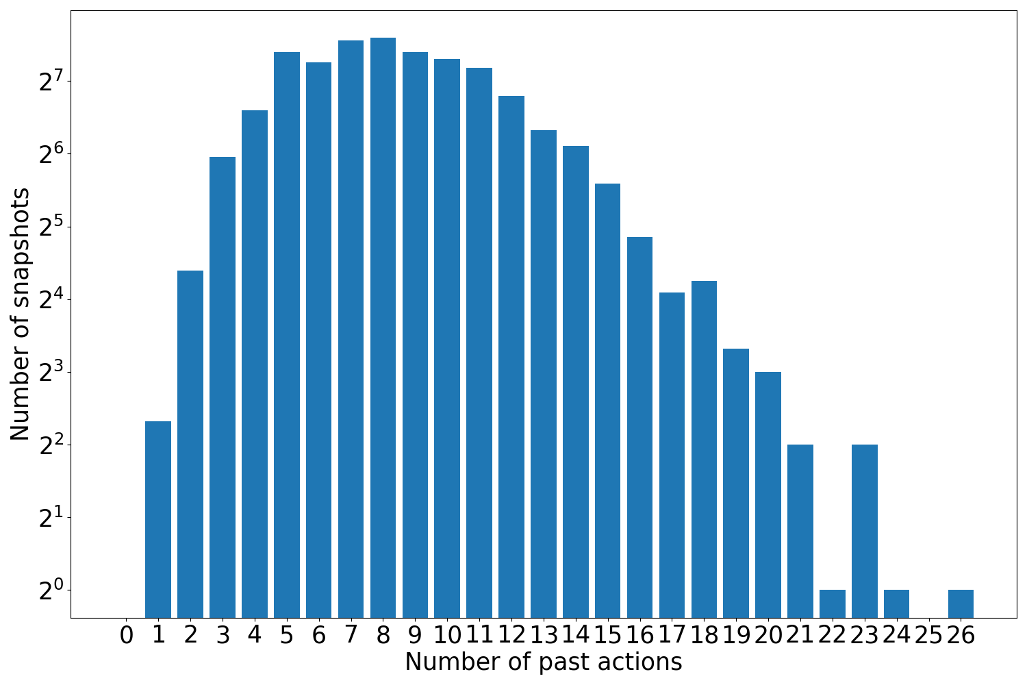
### Visual Description
## Bar Chart: Number of Snapshots vs. Number of Past Actions
### Overview
The image is a bar chart showing the distribution of snapshots based on the number of past actions. The x-axis represents the number of past actions, ranging from 0 to 26. The y-axis represents the number of snapshots, displayed on a logarithmic scale (base 2). The chart shows a distribution that initially increases, peaks around 7-9 past actions, and then decreases.
### Components/Axes
* **X-axis:** "Number of past actions" - Ranges from 0 to 26 in integer increments.
* **Y-axis:** "Number of snapshots" - Logarithmic scale (base 2) with markers at 2<sup>0</sup>, 2<sup>1</sup>, 2<sup>2</sup>, 2<sup>3</sup>, 2<sup>4</sup>, 2<sup>5</sup>, 2<sup>6</sup>, and 2<sup>7</sup>.
* **Bars:** Blue bars representing the number of snapshots for each number of past actions.
### Detailed Analysis
Here's a breakdown of the approximate values for the number of snapshots at different numbers of past actions. Note that these are approximate due to the logarithmic scale and visual estimation:
* **0 past actions:** Approximately 2<sup>2</sup> = 4 snapshots
* **1 past action:** Approximately 2<sup>2.2</sup> = 4.6 snapshots
* **2 past actions:** Approximately 2<sup>3.2</sup> = 9.2 snapshots
* **3 past actions:** Approximately 2<sup>4.3</sup> = 19.8 snapshots
* **4 past actions:** Approximately 2<sup>5.5</sup> = 45.3 snapshots
* **5 past actions:** Approximately 2<sup>6.5</sup> = 90.5 snapshots
* **6 past actions:** Approximately 2<sup>7</sup> = 128 snapshots
* **7 past actions:** Approximately 2<sup>7.2</sup> = 144 snapshots
* **8 past actions:** Approximately 2<sup>7.2</sup> = 144 snapshots
* **9 past actions:** Approximately 2<sup>7.1</sup> = 135 snapshots
* **10 past actions:** Approximately 2<sup>7</sup> = 128 snapshots
* **11 past actions:** Approximately 2<sup>6.8</sup> = 110 snapshots
* **12 past actions:** Approximately 2<sup>6.6</sup> = 95 snapshots
* **13 past actions:** Approximately 2<sup>6.3</sup> = 75 snapshots
* **14 past actions:** Approximately 2<sup>6</sup> = 64 snapshots
* **15 past actions:** Approximately 2<sup>5.6</sup> = 48 snapshots
* **16 past actions:** Approximately 2<sup>5.2</sup> = 36 snapshots
* **17 past actions:** Approximately 2<sup>4.8</sup> = 28 snapshots
* **18 past actions:** Approximately 2<sup>4.5</sup> = 22.6 snapshots
* **19 past actions:** Approximately 2<sup>3.8</sup> = 13.9 snapshots
* **20 past actions:** Approximately 2<sup>3.3</sup> = 9.8 snapshots
* **21 past actions:** Approximately 2<sup>2.8</sup> = 6.9 snapshots
* **22 past actions:** Approximately 2<sup>0.8</sup> = 1.7 snapshots
* **23 past actions:** Approximately 2<sup>2</sup> = 4 snapshots
* **24 past actions:** Approximately 2<sup>0.2</sup> = 1.1 snapshots
* **25 past actions:** Approximately 2<sup>0.2</sup> = 1.1 snapshots
* **26 past actions:** Approximately 2<sup>0</sup> = 1 snapshot
### Key Observations
* The distribution is unimodal, with a peak between 6 and 9 past actions.
* The number of snapshots increases rapidly from 0 to around 7 past actions.
* The number of snapshots decreases more gradually after the peak.
* There are relatively few snapshots with a very low or very high number of past actions.
### Interpretation
The chart suggests that the system being analyzed tends to operate with a moderate number of past actions. The peak in the distribution indicates that this range is the most common or stable state for the system. The rapid increase and gradual decrease could indicate that the system quickly reaches a stable state but takes longer to transition out of it. The low number of snapshots at the extremes suggests that these states are either rare or short-lived.
</details>
Figure 7: Number of snapshots (in $log_{2}$ ) for sets of $n$ past actions in the Action Genome test set. (a) – Abduct at $T$ , (b) – Abduct last snapshot
.
How to generate action sets and sequences? To obtain the ground truth action set $\mathcal{A}$ for an image in the Action Genome dataset using the Charades action labels, we first compute the time $t$ for each individual frame within a video sequence by using the formula: ${t}=\frac{v_{d}}{n}$ , where $v_{d}$ and $n$ denote the video duration and the number of frames in the video respectively. Then, we multiply the current frame number $f_{n}$ with ${t}$ to obtain the current time, $t_{c}=t× f_{n}$ .
Action sets: As each video contains multiple actions, we check whether the current time of the frame $t_{c}$ , falls within the start $t_{s}$ and end $t_{e}$ time of the action. If it does, we add the ground truth action label to the action set $\mathcal{A}_{n}$ for the image. To obtain the ground truth action set for the $t^{th}$ image, we combine all previous action sets from $t=1$ up to and including the $t^{th}$ image to form the set.
Action sequences: We sort the start time $t_{s}$ of the actions contained in the video in ascending order. Then, for each image, if the current time of the frame is greater than the start time of the action ( $t_{c}≥ t_{s}$ ), we add it to the sequence.
We provide details on the number of images for a set of $n$ past actions in the AG dataset for these setups in Figure 7. As can be seen from these statistics, the majority of the images have more than five actions and some images have as many as 26 actions.
8 Implementation Details
We use FasterRCNN [36] with a ResNet-101 [17] backbone to extract human and object features from each image based on the ground truth person and object bounding boxes provided by AG for all object-relational models. We load pre-trained weights provided by [5] that were trained on the training set of AG which obtained 24.6 mAP at 0.5 IoU with COCO metrics. The parameters of the FasterRCNN during training and inference are fixed for the abductive past action inference task. Our default human and object visual representations have 512 dimensions obtained from 2048 dimensional visual features from the FasterRCNN. We use linear mappings to do this. During training, we train the models for 10 epochs and set the batch size to 1 video (there are many frames in a video). We assume the frames are i.i.d. Note that even though there are multiple images in a batch, the images are processed in parallel and individually for the transformer and graph models respectively. There is no sharing of information between images. We use the AdamW [28] optimizer with an initial learning rate of 1e-5 along with a scheduler to decrease the learning rate by a factor of 0.5 to a minimum of 1e-7. We utilize Glove [32] word embedding of size 200 for the human and object semantic features. In addition, gradient clipping with a maximal norm of 5 is applied. Moreover, we report the mean across 3 different runs for each configuration to ensure we report the most accurate performance of our models. All models (except end-to-end and ViT) are trained on a single RTX3090 or A5000 GPU. For CLIP, we use publicly available implementations [33]. We use the public API of OpenAI for GPT 3.5 models.
9 Additional Experiments
9.1 Abductive Past Action Sequence Prediction
Next, we formulated the abductive past action sequence prediction task based on the Abduct at T setup. We attached a GRU / transformer decoder to our existing object-relational models. To train both sequence prediction models, we freeze the object detector and relational model ( $\phi()$ ). Then, we use the relational vector $x_{r}$ and action distribution obtained from $\phi_{c}()$ as the initial hidden state and pass it to the GRU respectively. The transformer decoder takes non-pooled relational features (a matrix of size $n× d$ ) as the key, value, and max-pooled relational features $x_{r}$ as the query. The output of these models is fed into a linear classifier to produce action sequences autoregressively. The results of these models are reported in Table 5. The BiGED model obtains slightly better performance than the rest. Although the performances of these models are suboptimal, we note that humans are also unable to obtain satisfactory results (only 14.00% accuracy). As we are constrained to only utilize available information in a single frame, the solution contains a substantial amount of sequence permutations. Therefore, the task is extremely challenging. The poor human performance also suggests how humans may use abduction. Perhaps humans do not resolve causal chains when performing abduction as it is a very challenging task.
We use the Hamming Loss to evaluate the action sequence prediction models as follows:
$$
H=\frac{1}{N*L}\sum_{n=1}^{N}\sum_{l=1}^{L}\left[y_{l}\neq\hat{y}_{l}\right] \tag{15}
$$
where $N$ is the total number of samples and $L$ is the sequence length. Finally, for a given sample, the accuracy is $(1-H)× 100$ .
Table 5: Abductive past action sequence prediction using the proposed methods on the Abduct at $T$ setup.
| Model Human performance | Accuracy 14.00 GRU | Transformer |
| --- | --- | --- |
| Relational MLP | 9.43 $±$ 0.13 | 9.59 $±$ 0.06 |
| Relational Self Att. Transformer | 9.72 $±$ 0.06 | 9.95 $±$ 0.07 |
| Relational Cross Att. Transformer | 9.69 $±$ 0.18 | 9.96 $±$ 0.12 |
| Relational GNNED | 9.81 $±$ 0.05 | 10.11 $±$ 0.19 |
| RBP | 10.48 $±$ 0.05 | 10.22 $±$ 0.12 |
| BiGED | 10.54 $±$ 0.15 | 10.1 $±$ 0.14 |
9.2 Ablation Study
Ablation on graph affinity function: By default, we use the Jaccard Vector Similarity as the affinity $W_{A}(i,j)$ for the GNNED and BiGED models. Here, we ablate the impact of this design choice by comparing it with cosine similarity and dot product. As can be seen from the results in Table 6, the Jaccard Vector Similarity (JVS) obtains better results than cosine similarity and dot product. This behavior can be attributed to the fully differentiable and bounded nature of JVS in contrast to the dot product or cosine similarity.
Table 6: Ablation on graph affinity using Abduct at T setup.
| Jaccard Vector Similarity Cosine Similarity Dot product | 35.75 34.17 28.81 | 60.55 57.98 54.68 | 44.37 41.97 38.38 |
| --- | --- | --- | --- |
Impact of semantic features and learning scheduler: Apart from the two different setups mentioned, we also use a third setup for ablations. In the third setup, the action sets are formed from the current and previous images which form the ground truth denoted by $\mathcal{A}=\{\mathcal{A}_{t-1}\bigcup\mathcal{A}_{t}\}$ for faster experimentation. We retrain all object-relational models with the corresponding past action set obtained from the current and previous images. We perform ablation studies on the relational self-attention transformer based on this setup. These findings can also be generalized to the other setups as mentioned earlier.
We evaluate the effect of visual and semantic (Glove [32]) features in Table 7. The use of semantic features provides a huge performance boost across all metrics. We attribute the performance increase to the contextual information provided by the semantics. The semantics of objects enable the model to effectively identify and relate actions, providing a more intuitive means for reasoning about these actions. It is also interesting to see the impact of the learning rate scheduler which provides considerable improvement for the transformer model. Therefore, we use semantics and the learning rate scheduler for all our models.
Table 7: Ablation study for the impact of semantic features and scheduler on the abductive past action set inference for the Abduct from current and previous images setup using self-attention transformer.
| Visual only Visual + scheduler Visual + semantic | 21.42 $±$ 0.13 21.93 $±$ 0.16 35.40 $±$ 0.16 | 46.44 $±$ 0.12 47.04 $±$ 0.44 68.47 $±$ 0.06 | 34.24 $±$ 0.42 34.80 $±$ 0.47 54.90 $±$ 0.52 |
| --- | --- | --- | --- |
| Visual + semantic + scheduler | 35.77 $±$ 0.30 | 69.16 $±$ 0.50 | 55.70 $±$ 0.47 |
9.3 Object-Relational Model Parameters
Table 8: The object-relational model parameters for the abductive past action inference task.
| Relational MLP Relational Self Att. Transformer Relational Cross Att. Transformer | 13.4M 101.2M 65.9M |
| --- | --- |
| Relational GNNED | 80.7M |
| RBP | 373.4M |
| BiGED | 213.6M |
The proposed object-relational model parameters are shown in Table 8. The rule-based inference model does not have any parameters and is therefore omitted from the table. Based on the results shown earlier, we note that the GNNED model obtains better performance than the transformer model even though it has lesser parameters. In addition, our proposed BiGED model has lesser parameters and performs comparable to or better than the RBP model. These further demonstrate the effectiveness of the proposed GNNED, RBP, and BiGED models for the challenging task of abductive past action inference.
|
<details>
<summary>extracted/6142422/images/Comparison/000138_bbox.png Details</summary>
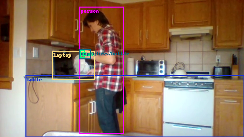
### Visual Description
## Object Detection: Kitchen Scene
### Overview
The image is a photograph of a kitchen scene with object detection bounding boxes overlaid. The objects detected are a person, a laptop, a cup/glass/bottle, and a table.
### Components/Axes
* **Bounding Boxes:**
* Pink: "person"
* Yellow: "laptop"
* Teal: "cup/glass/bottle"
* Blue: "table"
### Detailed Analysis or ### Content Details
* **Person:** A person is standing in the kitchen, wearing a red and white checkered shirt and jeans. The pink bounding box encompasses the entire person.
* **Laptop:** A laptop is on the counter to the left of the person. The yellow bounding box surrounds the laptop.
* **Cup/Glass/Bottle:** A cup, glass, or bottle is on the counter near the laptop. The teal bounding box surrounds the object.
* **Table:** The blue bounding box encompasses the counter, cabinets, and floor, labeling it as a table.
### Key Observations
* The object detection seems to be identifying common kitchen objects.
* The bounding boxes are generally well-placed around the identified objects.
### Interpretation
The image demonstrates an object detection system's ability to identify and locate objects within a kitchen environment. The system correctly identifies a person, a laptop, a cup/glass/bottle, and a table. The bounding boxes provide a visual representation of the system's confidence in its object localization.
</details>
| | | | | | | |
| --- | --- | --- | --- | --- | --- | --- | --- |
| Taking a cup/glass/bottle from somewhere | | | | | | | |
| Holding a cup/glass/bottle of something | | | | | | | |
| Working/Playing on a laptop | | | | | | | |
| Working at a table | | | | | | | |
| Watching a laptop or something on a laptop | | | | | | | |
| Drinking from a cup/glass/bottle | | | | | | | |
| Taking a cup/glass/bottle from somewhere | | | | | | | |
| Sitting at a table | | | | | | | |
| Working at a table | | | | | | | |
| Working/Playing on a laptop | | | | | | | |
| Holding a laptop | | | | | | | |
| Opening a laptop | | | | | | | |
| Sitting in a chair | | | | | | | |
| Drinking from a cup/glass/bottle | | | | | | | |
| Taking a dish/es from somewhere | | | | | | | |
| Putting something on a shelf | | | | | | | |
| Walking through a doorway | | | | | | | |
| Closing a closet/cabinet | | | | | | | |
| Opening a closet/cabinet | | | | | | | |
| Putting a dish/es somewhere | | | | | | | |
| Taking a dish/es from somewhere | | | | | | | |
| Someone is smiling | | | | | | | |
| Someone is sneezing | | | | | | | |
| Someone is standing up from somewhere | | | | | | | |
| Taking a cup/glass/bottle from somewhere | | | | | | | |
| Putting something on a table | | | | | | | |
| Closing a closet/cabinet | | | | | | | |
| Opening a closet/cabinet | | | | | | | |
| Putting a dish/es somewhere | | | | | | | |
| Taking a dish/es from somewhere | | | | | | | |
| Someone is cooking something | | | | | | | |
| Someone is smiling | | | | | | | |
| Someone is standing up from somewhere | | | | | | | |
| Taking a cup/glass/bottle from somewhere | | | | | | | |
| Putting something on a table | | | | | | | |
| Working/Playing on a laptop | | | | | | | |
| Tidying up a table | | | | | | | |
| Putting a cup/glass/bottle somewhere | | | | | | | |
| Drinking from a cup/glass/bottle | | | | | | | |
| Putting a dish/es somewhere | | | | | | | |
| Taking a dish/es from somewhere | | | | | | | |
| Someone is standing up from somewhere | | | | | | | |
| Taking a cup/glass/bottle from somewhere | | | | | | | |
| Holding a cup/glass/bottle of something | | | | | | | |
| Working/Playing on a laptop | | | | | | | |
| Putting something on a table | | | | | | | |
| Watching a laptop or something on a laptop | | | | | | | |
| Drinking from a cup/glass/bottle | | | | | | | |
| Putting a cup/glass/bottle somewhere | | | | | | | |
| Opening a closet/cabinet | | | | | | | |
| Taking a dish/es from somewhere | | | | | | | |
| Taking a cup/glass/bottle from somewhere | | | | | | | |
| Holding a cup/glass/bottle of something | | | | | | | |
| Working/Playing on a laptop | | | | | | | |
| Putting something on a table | | | | | | | |
| Walking through a doorway | | | | | | | |
| Putting a cup/glass/bottle somewhere | | | | | | | |
| Putting a dish/es somewhere | | | | | | | |
| Taking a dish/es from somewhere | | | | | | | |
| Someone is standing up from somewhere | | | | | | | |
|
<details>
<summary>extracted/6142422/images/Comparison/XOOTA.mp4/000102_bbox.png Details</summary>
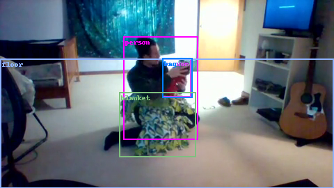
### Visual Description
## Object Detection: Indoor Scene with Person and Baby
### Overview
The image depicts an indoor scene with a person holding a baby, seated on a blanket on the floor. The image includes object detection bounding boxes around the identified objects.
### Components/Axes
* **Objects Detected:**
* Person (magenta bounding box)
* Baby (blue bounding box)
* Blanket (green bounding box)
* Floor (light blue bounding box)
### Detailed Analysis or ### Content Details
* **Person:** A person is seated on the floor, holding a baby. The person is wearing a dark-colored shirt.
* **Baby:** The baby is being held by the person. The baby is wrapped in a red blanket.
* **Blanket:** A patterned blanket is spread out on the floor, upon which the person is seated. The blanket has a mix of green, white, and blue colors.
* **Floor:** The floor is light-colored.
* **Background:** The background includes a TV on a shelf, a guitar, a door, and a curtain.
### Key Observations
* The object detection seems accurate, with bounding boxes correctly identifying the person, baby, blanket, and floor.
* The scene appears to be a casual indoor setting, possibly a living room or bedroom.
### Interpretation
The image demonstrates a successful object detection scenario in an indoor environment. The bounding boxes provide a clear indication of the identified objects and their locations within the scene. The context suggests a domestic setting with a person caring for a baby.
</details>
| | | | | | | |
| Holding a bag | | | | | | | |
| Snuggling with a blanket | | | | | | | |
| Sitting on the floor | | | | | | | |
| Lying on the floor | | | | | | | |
| Holding a vacuum | | | | | | | |
| Someone is awakening somewhere | | | | | | | |
| Taking a broom from somewhere | | | | | | | |
| Throwing a broom somewhere | | | | | | | |
| Tidying up with a broom | | | | | | | |
| Fixing a light | | | | | | | |
| Turning on a light | | | | | | | |
| Turning off a light | | | | | | | |
| Drinking from a cup/glass/bottle | | | | | | | |
| Holding a cup/glass/bottle of something | | | | | | | |
| Pouring something into a cup/glass/bottle | | | | | | | |
| Holding some clothes | | | | | | | |
| Putting clothes somewhere | | | | | | | |
| Holding a towel/s | | | | | | | |
| Putting a blanket somewhere | | | | | | | |
| Taking a blanket from somewhere | | | | | | | |
| Walking through a doorway | | | | | | | |
| Someone is smiling | | | | | | | |
| Someone is sneezing | | | | | | | |
| Someone is standing up from somewhere | | | | | | | |
| Holding a bag | | | | | | | |
| Holding some clothes | | | | | | | |
| Putting clothes somewhere | | | | | | | |
| Taking some clothes from somewhere | | | | | | | |
| Opening a bag | | | | | | | |
| Taking a bag from somewhere | | | | | | | |
| Walking through a doorway | | | | | | | |
| Someone is smiling | | | | | | | |
| Someone is standing up from somewhere | | | | | | | |
| Holding a bag | | | | | | | |
| Snuggling with a blanket | | | | | | | |
| Opening a bag | | | | | | | |
| Putting a bag somewhere | | | | | | | |
| Taking a bag from somewhere | | | | | | | |
| Putting a blanket somewhere | | | | | | | |
| Taking a blanket from somewhere | | | | | | | |
| Tidying up a blanket/s | | | | | | | |
| Someone is standing up from somewhere | | | | | | | |
| Holding a bag | | | | | | | |
| Snuggling with a blanket | | | | | | | |
| Sitting on the floor | | | | | | | |
| Holding a vacuum | | | | | | | |
| Opening a bag | | | | | | | |
| Taking a bag from somewhere | | | | | | | |
| Taking a blanket from somewhere | | | | | | | |
| Drinking from a cup/glass/bottle | | | | | | | |
| Tidying something on the floor | | | | | | | |
| Holding a bag | | | | | | | |
| Snuggling with a blanket | | | | | | | |
| Sitting on the floor | | | | | | | |
| Holding a vacuum | | | | | | | |
| Opening a bag | | | | | | | |
| Taking a bag from somewhere | | | | | | | |
| Throwing a blanket somewhere | | | | | | | |
| Fixing a vacuum | | | | | | | |
| Someone is standing up from somewhere | | | | | | | |
Figure 8: Manually selected qualitative results produced by each model on the abductive past action set inference: Abduct last image setup on the AG test dataset. The first column shows the image followed by their corresponding ground truth past actions. The remaining columns display the actions predicted by each model, with correct predictions highlighted in green and incorrect predictions highlighted in red.
9.4 Qualitative Results
We compare qualitative results for the abductive past action set prediction task in Figure 8. Depending on the number of past action labels an image has, we take the same number of top-k predicted actions from each model. All models demonstrate their ability to perform abductive past action inference. In the first image, there are objects such as a person, laptop, table, cup, and dish. In the second image, there are objects such as a person, floor, blanket, bag, and vacuum. In both scenarios, RBP and BiGED demonstrate that they can infer past actions more accurately.