## TPU-MLIR: A Compiler For TPU Using MLIR
Pengchao Hu Man Lu Lei Wang Guoyue Jiang pengchao.hu,man.lu,lei.wang,guoyue.jiang } @sophgo.com
{ Sophgo Inc.
## Abstract
Multi-level intermediate representations (MLIR) show great promise for reducing the cost of building domain-specific compilers by providing a reusable and extensible compiler infrastructure. This work presents TPU-MLIR, an end-to-end compiler based on MLIR that deploys pre-trained neural network (NN) models to a custom ASIC called a Tensor Processing Unit (TPU). TPU-MLIR defines two new dialects to implement its functionality: 1. a Tensor operation (TOP) dialect that encodes the deep learning graph semantics and independent of the deep learning framework and 2. a TPU kernel dialect to provide a standard kernel computation on TPU. A NN model is translated to the TOP dialect and then lowered to the TPU dialect for different TPUs according to the chip's configuration. We demonstrate how to use the MLIR pass pipeline to organize and perform optimization on TPU to generate machine code. The paper also presents a verification procedure to ensure the correctness of each transform stage.
## 1. Introduction
The development of deep learning (DL) has profoundly impacted various scientific fields, including speech recognition, computer vision, and natural language processing. In order to facilitate the process of training deep learning models, industry and academia have developed many frameworks, such as Caffe, Tensorflow, Pytorch, Mxnet, and PaddlePaddle, which boost deep learning in many areas. However, each framework has its proprietary graph representation, which brings lots of work for deploying as we need to support many DL model formats.
At the same time, matrix multiplication and high dimensional tensor convolution are the heavy computation in DL, which evoke the passion of chip architects to design customized DL accelerators to achieve high performance at low energy. Although GPU is still the leading hardware in training DL models and all the
DL frameworks have contributed much work to support this general-purpose hardware, GPU is not the perfect piece in the inference domain of DL. GPU is for gaming, graph rendering, scientific computation, and much more, not tailored for DL only. Thus, many DL accelerators, such as Google TPU, Apple Bonic, Graphcore IPU, and SOPHGO TPU, are more energy efficient than GPU and benefit many of these emerging DL applications.
In addition, the DL community has resorted to domain-specific compilers for rescue to address the drawback of DL libraries and alleviate the burden of manually optimizing the DL models on each DL hardware. The DL compilers take the model described in the DL frameworks as inputs and generate efficient code for various DL hardware as outputs. The transformation between a model definition and specific code implementation is highly optimized, considering the model specification and hardware architecture. Several popular DL compilers, such as TVM, Tensor Comprehension, and XLA, have been proposed by industry and academia. Specifically, they incorporate DL-oriented optimizations such as layer and operator fusion, which enables highly efficient code generation.
Herein, We provide TPU-MLIR, an open-source DL compiler for TPU. In particular, we chose Open Neural Network Exchange (ONNX)[1] as a DL format to represent our compiler's input model and use Multi-level Intermediate Representation (MLIR) [7], a modern opensource compiler infrastructure for multi-level intermediate representation, to design TPU-MLIR 1 compiler.
In this work, we will introduce our compiler by
- presenting the overall design and architecture of the compiler,
- introducing two new dialects: TOP dialect to encode the deep learning graph semantics independent of the deep learning framework and TPU dialect to provide a common lowering point for all TOP dialect operations but device-dependent,
1 https://github.com/sophgo/tpu-mlir
- detailing each compile stage, such as converting NN models to Top dialect as device independent and then converting TOP to TPU for various chips and types,
- defining WeightOp for weight operation and store weight data in the NumPy npz file, and
- providing InferenceInterface for TOP and TPU to ensure correct conversions.
We organize the remainder of the paper as follows. In Sec. 2, we briefly discuss MLIR, ONNX, on which our compiler is based, and the calibration processing, which tailors computation for TPU. Sec. 3, we introduce our compiler's design principle and architecture and discuss TOP and TPU dialects. We also discuss using inference to ensure correctness in each conversion stage. Finally, we conclude our paper and discuss future work in Sec. 4.
## 2. Background
## 2.1. MLIR
The MLIR, with much reusable and extensible, is a novel approach for constructing new domain-specific compilers. An open ecosystem is the most significant difference from LLVM. MLIR standardizes the Static Single Assignment (SSA)-based IR data structures allowing one to express a range of concepts as first-class operations. Operations can represent many different levels of abstraction and computations, from dataflow graphs to target-specific instructions and even hardware circuitry. They take and produce zero or more values, called operands and results, respectively. A value represents data at runtime and is associated with a type known at compile-time, whereas types model compile-time information about values. Complementary to this, attributes contain compile-time information to operations. Operations, Attributes, and type systems are open and extensible. The custom types, operations, and attributes are logically grouped into dialects. A dialect is one of the most fundamental aspects of MLIR that enables the infrastructure to implement a stack of reusable abstractions. Each abstraction encodes and preserves transformation validity preconditions directly in its IR, reducing the complexity and cost of analysis passes. The MLIR IR has a recursive structure where operations contain a list of regions, and regions contain a list of blocks, which in turn, contain a list of operations.
In particular, MLIR features operation, attribute and type interfaces providing a generic way of interacting with the IR. Interfaces allow transformations and analyses to work with abstract properties rather than fixed lists of supported concepts. Interfaces can be implemented separately from operations and mixed in using MLIR's registration mechanism, thus fully separating IR concepts from transformations. Furthermore, transformations can be written as compositions of orthogonal localized 'match and rewrite' primitives. These are often decomposed further into rewriting rules when applied within a dialect and lowering rules when converting from a higher-level dialect to a lower-level dialect. Throughout the compilation, separate dialects can co-exist to form a hybrid program representation. The ability to progressively lower dialects to the target hardware during the compilation process has made MLIR an excellent compiler infrastructure for domainspecific languages.
This article relies on several MLIR dialects and types, briefly described below.
## 2.1.1 Ranked Tensor Type
Values with tensor type represent aggregate Ndimensional homogeneous data indicated by element type and a fixed rank with a list of dimensions 2 . Each dimension could be a static non-negative integer constant or be dynamically determined (marked by ? ).
This abstracted runtime representation carries both the tensor data values and information about the tensor shape, but the compiler has not decided on its representation in memory. Tensor values are immutable and subject to def-use SSA semantics[9]. Operations on tensors are often free of side effects, and operations always create new tensors with a value. The textual format of the tensor is tensor 〈 d 1 xd 2 x · · · xd N xdtype 〉 , where d 1 , d 2 , ... d N are integers or symbol ? representing the dimensions of a tensor, and dtype is the type of the elements in a tensor, e.g., F32 for float32. A tensor can be unranked when its shapes are unknown. MLIR uses tensor 〈∗ xdtype 〉 to represent unranked tensor types.
## 2.1.2 Quantization Dialect
Quantization dialect 3 provides a family of quantized types and type-conversion operations. The 'quantization' refers to the conversion of floating-point computations to corresponding variants expressed in integer math for inference, as has been supported by lowbit depth inference engines such as various accelerator hardware and many DSPs. There are three types defined in quantization dialect: UniformQuantizedType, UniformQuantizedPerAxisType, and CalibratedQuantizedType. The UniformQuantizedType and Unifor-
2 https://mlir.llvm.org/docs/Dialects/Builtin/#rankedtensortype
3 https://mlir.llvm.org/docs/Dialects/QuantDialect
mQuantizedPerAxisType represent the mapping between expressed values (e.g., a floating-point computer type) and storage values (typically of an integral computer type), expressing the affine transformations from uniformly spaced points to the real number line. The relationship is: realValue = scale × ( quantizedValue -zeroPoint ) and will be discussed in more detail in Section 2.3. Where CalibratedQuantizedType holds the range from the given min and max value of the histogram data of the tensor, used for recording the statistics information of the tensor. The UniformQuantizedPerAxisType applies affine transformation individually to each index along a specific axis of a tensor type. However, UniformQuantizedType applies the affine transformation to every value within the target type. The type-conversion defined in quantization dialect provides three operations for converting between types based on a QuantizedType and its expressed and storage sub-types. Those operations are: quant . qcast converting from an expressed type to QuantizedType, quant . dcast converting from a QuantizedType to its expressed type, and quant . scast converting between a QuantizedType and its storage type.
## 2.2. ONNX
ONNX is an open-source framework-independent format widely used for exchanging computation graph models, including deep learning and traditional machine learning. It was accepted as a graduate project in Linux Foundation AI and maintained by open-source communities. ONNX defines an extensible computation graph model, operators, and standard data types for deep learning and provides a set of specifications to convert a model to a basic ONNX format and another to get the model back from this ONNX form. It is an ideal tool for framework interoperability, especially when deploying a model to specific hardware[5].
ONNX reduces the friction of moving trained DL models among AI frameworks and platforms. ONNX uses the Protocol Buffers language for its syntax and provides rich documents and tools to formalize each operation's semantics and verify its correctness.
## 2.3. Quantization
Quantization is a promising technique to reduce deep learning models' memory footprint, inference latency, and power consumption, which replaces highcost floating-point (always F32) computation with low-cost fixed-point numbers[4] (e.g., INT8/INT16) or float-point (e.g., BF16/F16). Because most current DL models are heavily over-parameterized and robust to extreme discretization, there is much opportunity for reducing numeral precision without impact- ing the model's accuracy, bringing ample search space for tuning. Although many quantization methods have emerged, there is not a single well-posed or wellconditioned problem being solved[3]. Instead, one is interested in some error metric (based on classification quality, data similarity, etc.). to guide the quantization process. However, due to the over-parameterization, it is possible to have a high error between a quantized and the original model while still attaining excellent generalization performance. Finally, different layers in a Neural Net have a different impact on the loss function, which motivates a mixed-precision approach quantization.
## 2.3.1 Uniform Quantization
The quantization process is a function mapping from real values r to some numeral values. Quantization function such as
<!-- formula-not-decoded -->
where quant is the quantization operator, r is a realvalued input (activation or weight), s is a float-point scaling factor, and zp is an integer zero point, is known as uniform quantization, as the resulting quantized values are evenly spaced.
## 2.3.2 Symmetric and Asymmetric Quantization
Acrucial factor in uniform Quantization is choosing the scaling factor s in Equation 1. This scaling factor, also known as resolution, divides a given range of real-values r into several partitions s = β -α 2 b -1 , where [ α, β ] denotes the clipping range that we are clipping the real-values with, and b is the quantization bit width[4][6]. Therefore, one should determine the clipping range [ α, β ] before generating the scaling factor. If the clipping range of α equals -β , we get Symmetric Quantization, and on the contrary, we get asymmetric Quantization. The asymmetric quantization method often results in a tighter clipping range than symmetric Quantization, which is especially important when the dynamic range of the tensor is imbalanced, e.g., the result of ReLU always has non-negative values.
## 2.3.3 Calibration
The process of choosing the clipping range is called 'calibration.' One popular method for pre-calculation is to run a series of inferences on some sample data and then get the distribution of each tensor in the graph. Using the min/max of the signal for both symmetric and asymmetric Quantization is typical in most
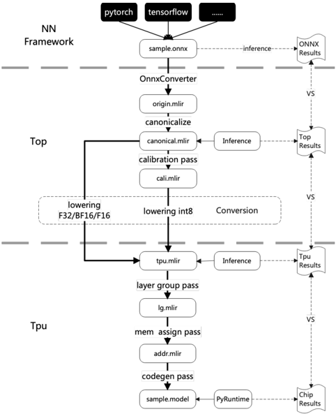
Figure 1: Architecture of tpu-mlir.
<details>
<summary>Image 1 Details</summary>
### Visual Description
## Diagram: NN Framework Conversion Pipeline
### Overview
The image is a flowchart illustrating the conversion pipeline of a neural network (NN) framework, starting from frameworks like PyTorch and TensorFlow, processing through ONNX conversion, and then optimizing for a TPU. The diagram shows the flow of data and processes, including lowering, inference, and conversion steps, with intermediate results being compared at various stages.
### Components/Axes
* **Header:** Contains the input frameworks (PyTorch, TensorFlow, and others represented by "...").
* **NN Framework:** Label indicating the initial stage of the pipeline.
* **Top:** Label indicating the intermediate stage of the pipeline.
* **Tpu:** Label indicating the final stage of the pipeline.
* **Nodes:** Rectangular boxes represent processes or data formats (e.g., "sample.onnx", "OnnxConverter", "origin.mlir").
* **Arrows:** Indicate the flow of data or control between processes. Solid arrows represent primary flow, dashed arrows represent inference or comparison.
* **Inference:** Dashed arrows labeled "inference" indicate inference processes.
* **VS:** Label indicating a comparison between the results of the main flow and the inference results.
* **Results:** Dashed arrows labeled "ONNX Results", "Top Results", "Tpu Results", and "Chip Results" indicate the results of the inference processes at different stages.
### Detailed Analysis
1. **Input Frameworks:**
* "pytorch" (top-left)
* "tensorflow" (top-center)
* "..." (top-right, indicating other frameworks)
2. **Initial Conversion:**
* "sample.onnx" (directly below the input frameworks)
* "OnnxConverter" (below "sample.onnx")
* "origin.mlir" (below "OnnxConverter")
* "canonicalize" (below "origin.mlir")
* "canonical.mlir" (below "canonicalize")
* "calibration pass" (below "canonical.mlir")
* "cali.mlir" (below "calibration pass")
3. **Lowering and Conversion:**
* "lowering F32/BF16/F16" (left side, in a rounded box)
* "lowering int8" (right side, in a rounded box)
* "Conversion" (right side, in a rounded box)
4. **TPU Optimization:**
* "tpu.mlir" (below the lowering/conversion stage)
* "layer group pass" (below "tpu.mlir")
* "lg.mlir" (below "layer group pass")
* "mem assign pass" (below "lg.mlir")
* "addr.mlir" (below "mem assign pass")
* "codegen pass" (below "addr.mlir")
* "sample.model" (below "codegen pass")
* "PyRuntime" (to the right of "sample.model")
5. **Inference and Comparison:**
* Dashed arrows labeled "inference" branch off from "sample.onnx", "canonical.mlir", and "tpu.mlir".
* Dashed arrows labeled "ONNX Results", "Top Results", "Tpu Results", and "Chip Results" indicate the results of the inference processes at different stages.
* "VS" labels indicate a comparison between the results of the main flow and the inference results.
### Key Observations
* The diagram illustrates a multi-stage conversion and optimization process for neural networks.
* The process involves converting models from different frameworks to ONNX format, then optimizing them for TPU deployment.
* Inference is performed at multiple stages, and the results are compared to the main flow to ensure accuracy.
* The diagram highlights the different passes and transformations applied to the model during the conversion process.
### Interpretation
The diagram depicts a typical workflow for deploying neural networks on TPUs. It starts with models defined in popular frameworks like PyTorch and TensorFlow. These models are first converted to the ONNX (Open Neural Network Exchange) format, which acts as an intermediary representation. The ONNX model then undergoes a series of optimization and transformation steps, including canonicalization, calibration, and lowering to specific data types (F32, BF16, F16, and int8). These steps are crucial for improving performance and reducing memory footprint on the TPU. The "inference" branches and "VS" comparisons suggest a validation process where the accuracy of the transformed model is checked against the original model at different stages. The final "sample.model" represents the optimized model ready for deployment on the TPU, using a PyRuntime environment. The entire process aims to leverage the specialized hardware capabilities of TPUs for efficient neural network execution.
</details>
cases. However, this approach is susceptible to outlier data in the activations, which could unnecessarily increase the range and reduce quantization resolution. One approach to address this is using percentile or selecting α and β to minimize KL divergence between the real and the quantized values[8][11]. Besides, there are other metrics to find the best range, including minimizing Mean Squared Error (MSE)[2], entropy, and cosine similarity.
## 3. Compiler
This section introduces the compiler, TPU-MLIR, which creates two layers by the TOP and TPU dialects for converting NN models to executable files by various types and chips. We discuss TPU-MLIR's overall architecture first.
## 3.1. Overview
Figure 1 shows the overall architecture of TPUMLIR. We divide it into the NN Framework, Top, and Tpu.
- 1) NN Framework : TPU-MLIR supports ONNX models directly. Other NN framework models, such as Pytorch, and Tensorflow, need to convert
to ONNX modes.
- 2) TOP : refer to the TOP dialect as the top abstraction level representing NN models in the MLIR language. It is device independent.
- 3) TPU : refer to the TPU dialect, which is the TPU abstraction level and represents TPU operations. It is device dependent.
We first convert a NN model to TOP abstraction with TOP dialect and built-in dialect defined in MLIR, which we call TOP mlir file, by python script, i.e., OnnxConverter in figure 1. Then we lower the top mlir file to TPU abstraction with TPU dialect and built-in dialect defined in MLIR, which we call tpu mlir through some passes, such as canonicalization pass and calibration pass. At last, we convert tpu mlir to tpu models by some passes, such as layer group pass and memory assign pass. These passes will be discussed in the later section.
## 3.2. Module
We introduce our module definition by a simple mlir file showed Listing 1:
Module has some attributes: module . name is related to the NN model name; module . weight file is a npz 4 file that stores weight data needed by operations. We use location to express operation name. For example, '%2 = 'top.Weight'()' (Line 6 in Listing 1) is a weight op, and location is 'filter conv1'. So the real weight data is stored in 'conv2d weight.npz' file by name 'filter conv1'.
## 3.3. Top Dialect
TOP dialect is very similar to TOSA (Tensor Operator Set Architecture) 5 dialect in MLIR. So why we don't use TOSA dialect? There are two reasons: the first is that we need to do inference for each operations, and may create some new features in the futrue; the second is that we need to keep extend capability to support various NN models.
TOP Dialect is defined as below:
```
```
4 https://numpy.org/neps/nep-0001-npy-format.html
https://www.mlplatform.org/tosa
```
```
Listing 1: Simple convolution computation represented by TPU dialect.
```
```
TOP Op has two interfaces: 'InferenceInterface' and 'FlopsInterface'. 'InferenceInterface' is used to do inference for operation, which would be introduced later. 'FlopsInterface' is used to count FLOPs (floating point operations) of operation, as we are interested in the FLOPs of a NN model, also we use it to evaluate chip performance after running on the chip.
There are top operations defined based on TOP BaseOp or TOP Op. Here just using ConvOp and WeightOp for examples.
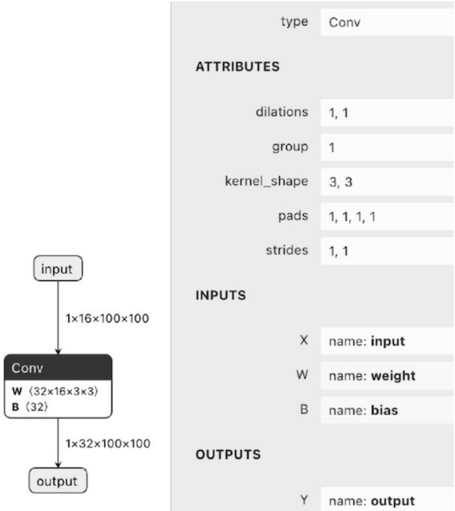
## 3.3.1 top::ConvOp
ConvOp is defined as below:
```
```
```
```
ConvOp represents conv operation of NN models, like Figure 2:
and in mlir file experessed as below:
```
```
## 3.3.2 top::WeightOp
WeightOp is a special operation for weight datas. Defined as below:
```
```
Figure 2: Convolution operation defined in ONNX.
<details>
<summary>Image 2 Details</summary>
### Visual Description
## Diagram: Convolutional Layer
### Overview
The image depicts a convolutional layer in a neural network, showing the input, the convolutional operation, and the output. It also includes the attributes, inputs, and outputs of the convolutional layer.
### Components/Axes
* **Left Side:** Flow diagram of the convolutional layer.
* **Input:** A rounded rectangle labeled "input".
* **Convolutional Layer:** A dark rectangle labeled "Conv" with "W (32x16x3x3)" and "B (32)" inside.
* **Output:** A rounded rectangle labeled "output".
* **Arrows:** Arrows indicating the flow of data from input to the convolutional layer and from the convolutional layer to output.
* **Dimensions:** "1x16x100x100" above the arrow from input to the convolutional layer, and "1x32x100x100" above the arrow from the convolutional layer to output.
* **Right Side:** Attributes, inputs, and outputs of the convolutional layer.
* **Type:** "Conv"
* **Attributes:**
* dilations: 1, 1
* group: 1
* kernel\_shape: 3, 3
* pads: 1, 1, 1, 1
* strides: 1, 1
* **Inputs:**
* X: name: input
* W: name: weight
* B: name: bias
* **Outputs:**
* Y: name: output
### Detailed Analysis or ### Content Details
* **Input:** The input has dimensions 1x16x100x100.
* **Convolutional Layer:**
* The convolutional layer is labeled "Conv".
* The weights (W) have dimensions 32x16x3x3.
* The bias (B) has dimensions 32.
* **Output:** The output has dimensions 1x32x100x100.
* **Attributes:**
* The dilations are 1, 1.
* The group is 1.
* The kernel shape is 3, 3.
* The pads are 1, 1, 1, 1.
* The strides are 1, 1.
* **Inputs:**
* The input (X) is named "input".
* The weights (W) are named "weight".
* The bias (B) is named "bias".
* **Outputs:**
* The output (Y) is named "output".
### Key Observations
* The input dimensions change from 1x16x100x100 to 1x32x100x100 after passing through the convolutional layer.
* The convolutional layer has weights of size 32x16x3x3 and a bias of size 32.
* The attributes of the convolutional layer define the parameters of the convolution operation.
### Interpretation
The diagram illustrates a single convolutional layer within a neural network. The input data, with dimensions 1x16x100x100, is processed by the convolutional layer, resulting in an output with dimensions 1x32x100x100. The convolutional layer's attributes, such as kernel shape, strides, and padding, determine how the convolution operation is performed. The weights and biases are the learnable parameters of the layer. The diagram provides a clear and concise representation of the structure and parameters of a convolutional layer, which is a fundamental building block in many deep learning models, particularly in computer vision. The change in dimensions from input to output (1x16x100x100 to 1x32x100x100) indicates that the convolutional layer is increasing the number of feature maps from 16 to 32.
</details>
WeightOp is corresponding to weight operation. Weight data is stored in 'module.weight file', WeightOp can read data from weight file by read method, or create new WeightOp by create method.
## 3.4. TPU Dialect
TPU Dialect is defined as below:
```
```
TPU dialect is for TPU chips, here we support SOPHGO AI chips first. It is used to generate chip command instruction sequences by tpu operations.
In TPU dialect, TPU BaseOp and TPU Op define as:
```
```
```
```
TPU Op has two interfaces, 'GlobalGenInterface' and 'InferenceInterface'. 'GlobalGenInterface' is used to generate chip command. 'InferenceInterface' is used to do inference for tpu operations.
There are top operations defined based on TOP BaseOp or TOP Op. Here using tpu::ConvOp , and tpu::CastOp, and tpu::GroupOp for example.
## 3.4.1 tpu::Conv2DOp
Conv2DOp is defined as below:
```
```
Compared to top::ConvOp, tpu::Conv2DOp has some new attributes: 'multiplier', 'rshift' and 'group info'. 'multiplier' and 'rshift' are used to do INT8 convolution after quantization, and not used if the convolution is float. 'group info' is used for the layer group. We will discuss layer group later.
## 3.4.2 tpu::CastOp
CastOp is defined as below:
```
```
```
```
Listing 2: top . cast operaiotn convertion a quant . calibrated type to quant . uniform type.
```
```
Listing 3: top . cast operaiotn convertion a quant . uniform type to float32 type.
CastOp is for transferring tensor type from one type to another. It can convert the F32 type to BF16[10] type or F16 type, or INT8 type, and the other way around is also OK.
Specially, if input is F32 type and output is quantization type, such as Listing 2, then:
<!-- formula-not-decoded -->
If input is quantization type and output is F32 type, such as Listing 3, then
<!-- formula-not-decoded -->
.
## 3.4.3 tpu::GroupOp
GroupOp is defined as below:
```
```
GroupOp contains serial operations that can inference in tpu local memory. We will discuss it later.
## 3.5. Conversion
This section we discuss how to convert top ops to tpu ops.
We define 'ConvertTopToTpu' pass like this:
```
```
There are there options: mode, chip and isAsymmetric.
- 1) mode : set quantization mode, e.g. INT8, BF16, F16 or F32. Types should be supported by the chip.
- 2) chip : set chip name. TPU operations will act by this chip.
- 3) isAsymmetric : if mode is INT8, set true for asymmetric quantization; false for symmetric quantization.
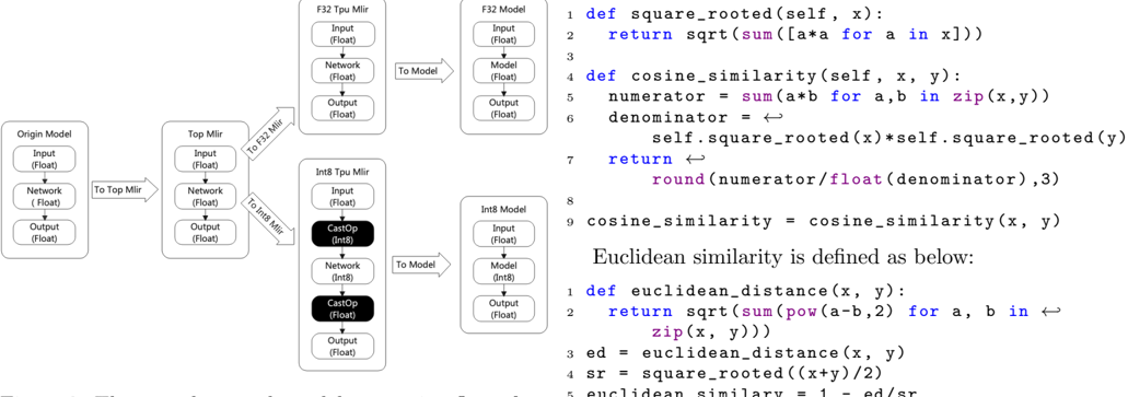
Typically, most attributes are the same after converting from TPU ops to TPU ops at float type (F32/BF16/F16). However, if the conversion is from float type to INT8 type, we should do PTQ (Posttraining Quantization)[4] at TOP dialect and add some external quantization attributes to TPU ops. At the same time, weight data, inputs, and outputs will be quantized to INT8. In addition, inputs and outputs
Figure 3: The neural network model conversion flow of TPU-MLIR.
<details>
<summary>Image 3 Details</summary>
### Visual Description
## Diagram: Model Conversion and Similarity Calculation
### Overview
The image presents a diagram illustrating the conversion of a model from its origin to different formats (F32 and Int8) using MLIR (Multi-Level Intermediate Representation). It also includes Python code snippets for calculating cosine similarity and Euclidean similarity.
### Components/Axes
**Model Conversion Diagram (Left Side):**
* **Origin Model:**
* Input (Float)
* Network (Float)
* Output (Float)
* **Top Mlir:**
* Input (Float)
* Network (Float)
* Output (Float)
* **F32 Tpu Mlir:**
* Input (Float)
* Network (Float)
* Output (Float)
* **F32 Model:**
* Input (Float)
* Model (Float)
* Output (Float)
* **Int8 Tpu Mlir:**
* Input (Float)
* CastOp (Int8) - Highlighted in black
* Network (Int8)
* CastOp (Float) - Highlighted in black
* Output (Float)
* **Int8 Model:**
* Input (Float)
* Model (Int8)
* Output (Float)
**Code Snippets (Right Side):**
* **Cosine Similarity:** Python code for calculating cosine similarity between two vectors.
* **Euclidean Similarity:** Python code for calculating Euclidean similarity.
**Arrows:**
* "To Top Mlir" - Connects Origin Model to Top Mlir.
* "To F32 Mlir" - Connects Top Mlir to F32 Tpu Mlir.
* "To Int8 Mlir" - Connects Top Mlir to Int8 Tpu Mlir.
* "To Model" - Connects F32 Tpu Mlir to F32 Model and Int8 Tpu Mlir to Int8 Model.
### Detailed Analysis
**Model Conversion Flow:**
1. The process starts with the **Origin Model**, which uses float data types.
2. The model is converted to **Top Mlir** format, still using float data types.
3. From Top Mlir, the model branches into two paths:
* **F32 Path:** The model is converted to **F32 Tpu Mlir**, then to the **F32 Model**. All components use float data types.
* **Int8 Path:** The model is converted to **Int8 Tpu Mlir**, where CastOp operations convert the data to Int8 and back to Float. Finally, it is converted to the **Int8 Model**.
**Code Snippets:**
* **Cosine Similarity:**
```python
1 def square_rooted(self, x):
2 return sqrt(sum([a*a for a in x]))
3
4 def cosine_similarity(self, x, y):
5 numerator = sum(a*b for a,b in zip(x,y))
6 denominator = self.square_rooted(x)*self.square_rooted(y)
7 return round(numerator/float(denominator),3)
8
9 cosine_similarity = cosine_similarity(x, y)
```
* **Euclidean Similarity:**
```python
Euclidean similarity is defined as below:
1 def euclidean_distance(x, y):
2 return sqrt(sum(pow(a-b,2) for a, b in zip(x, y)))
3 ed = euclidean_distance(x, y)
4 sr = square_rooted((x+y)/2)
5 euclidean similary = 1 - ed/sr
```
### Key Observations
* The diagram illustrates the process of converting a model into different numerical formats (F32 and Int8).
* The Int8 path involves CastOp operations to convert between Float and Int8 data types.
* The code snippets provide implementations for calculating cosine and Euclidean similarity.
### Interpretation
The diagram demonstrates a common workflow in model optimization, where a model is converted to lower-precision formats (like Int8) to improve performance and reduce memory footprint. The CastOp operations in the Int8 path are crucial for handling the data type conversions. The code snippets provide context by showing how similarity metrics can be calculated, potentially for evaluating the impact of the model conversion on its performance.
</details>
of a NN model need to insert CastOp if the convert type is not F32. The conversion flow chart shows in Figure 3.
## 3.6. Inference
This section discusses why we need inferences and how to support inferences for TOP and TPU dialects.
## 3.6.1 Why
TOP dialect run inference and get inference results, which has three uses.
- 1) It can be used to compare with original model results, to make sure NN model converts to TOP dialect correctly.
- 2) It can be used for calibration, which uses a few sampled inputs to run inference by top mlir file and get every intermediate result to stat proper min/max threshold used by Quantization.
- 3) It can be used to compare with the inference results tpu dialect to ensure tpu mlir is correct.
TPU dialect runs inference and gets inference results, which would compare with top mlir results. If tpu mlir is in F32 mode, the results should be the same. If tpu mlir is BF16/F16 mode, the tpu results may have some loss but should still have a good cosine ( > 0.95) and euclidean ( > 0.85) similarity. If tpu mlir is INT8 mode, cosine similarity should be greater than 0.9, and euclidean similarity should be greater than 0.5, based on experience. If the cosine similarity and euclidean similarity are not satisfied, the conversion correction from top to tpu is not guaranteed.
Cosine similarity is defined as below:
At last, after being compiled, the model can deploy in the tpu device and check the result with tpu mlir to ensure codegen is correct. If not similar, there are some bugs in codegen.
## 3.6.2 How
The NN models will run on NN runtime. For example, ONNX models can run on ONNX runtime. TOP dialect and TPU dialect run inference by 'InferenceInterface', which defines as below:
```
```
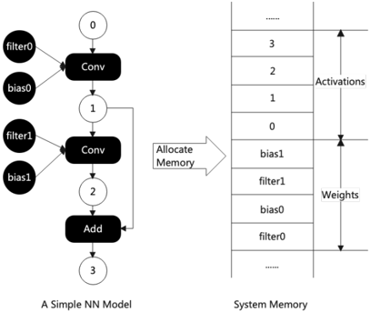
Figure 4: Buffer allocation in TPU-MLIR.
<details>
<summary>Image 4 Details</summary>
### Visual Description
## Diagram: Simple Neural Network Model and Memory Allocation
### Overview
The image presents a diagram illustrating a simple neural network (NN) model and its corresponding memory allocation in a system. The left side depicts the NN model's architecture, showing convolutional layers and an addition layer, along with filters and biases. The right side represents the system memory, indicating how activations and weights are stored. An arrow labeled "Allocate Memory" connects the NN model to the system memory, signifying the memory allocation process.
### Components/Axes
* **Left Side: A Simple NN Model**
* Nodes: Represented by circles with numbers (0, 1, 2, 3) indicating the sequence of operations.
* Layers: Convolutional layers ("Conv") and an addition layer ("Add") are represented by black rectangles.
* Inputs: "filter0", "bias0", "filter1", "bias1" are represented by black circles.
* Connections: Arrows indicate the flow of data between layers and inputs.
* **Right Side: System Memory**
* Memory Blocks: Represented by stacked rectangles, each containing a value or label.
* Activations: Labeled section of memory containing values 0, 1, 2, 3, and "...".
* Weights: Labeled section of memory containing "filter0", "bias0", "filter1", "bias1", and "...".
* Allocation Arrow: An arrow pointing from the NN model to the system memory, labeled "Allocate Memory".
### Detailed Analysis
* **NN Model Architecture:**
* Node 0: Input to the first convolutional layer ("Conv").
* Inputs to the first "Conv" layer are "filter0" and "bias0".
* Node 1: Output of the first "Conv" layer, input to the second "Conv" layer.
* Inputs to the second "Conv" layer are "filter1" and "bias1".
* Node 2: Output of the second "Conv" layer, input to the "Add" layer.
* The output of the first "Conv" layer (Node 1) is also fed back as input to the "Add" layer.
* Node 3: Output of the "Add" layer.
* **Memory Allocation:**
* The "Allocate Memory" arrow indicates that the NN model's parameters and intermediate results are stored in the system memory.
* The system memory is divided into two sections: "Activations" and "Weights".
* "Activations" store the intermediate results of the NN model's computations (0, 1, 2, 3).
* "Weights" store the model's parameters ("filter0", "bias0", "filter1", "bias1").
* The order of storage in the "Weights" section is "filter0", "bias0", "filter1", "bias1" from bottom to top.
### Key Observations
* The diagram illustrates a feedforward neural network with two convolutional layers followed by an addition layer.
* The memory allocation scheme shows a clear separation between activations and weights.
* The feedback loop from Node 1 to the "Add" layer (Node 2) suggests a recurrent or skip connection within the network.
### Interpretation
The diagram provides a simplified view of how a neural network model is implemented and how its data is stored in memory. The "Allocate Memory" arrow highlights the crucial step of assigning memory resources to the model's parameters (weights) and intermediate computations (activations). The separation of activations and weights in memory is a common practice in neural network implementations. The feedback loop in the NN model suggests a more complex architecture than a simple feedforward network, potentially incorporating recurrent or residual connections. The diagram demonstrates the relationship between the NN model's architecture and its memory footprint, which is essential for efficient implementation and deployment.
</details>
'inputs' and 'outputs' in 'InferenceParameter' point to input buffers and output buffers of the operation. All buffers that tensor needed would be allocated after mlir file were loaded. Each buffer size is calculated from Value's type. For example, the tensor 〈 1x32x100x100xf32 〉 needs 1 × 32 × 100 × 100 × sizeof ( float ) = 1280000 bytes . Figure 4 is an example.
Weights are allocated and loaded first, and then activations are allocated. Before inference, inputs of the model will be loaded to input buffers. And then, run inference. After inference, results are stored in each activation buffers.
'handle' in 'InferenceParameter' is used to point third-party excute engine, and it is optional.
'InferenceInterface' has three functions: 'init', 'inference', 'deinit'. 'init' and 'deinit' are used to init and deinit handle of third-party engine if needed, or do nothing. 'inference' is used to run inference with 'inputs' in 'InferenceParameter' and store results in 'outputs' of 'InferenceParameter'.
## 3.7. Layer Group
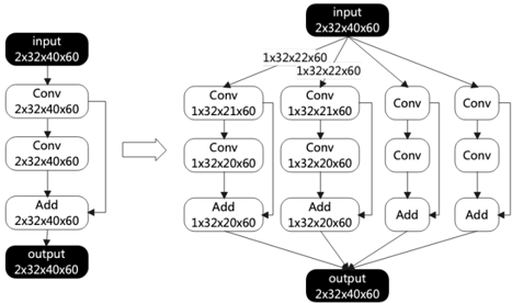
Layer group in TPU-MLIR means some layers composed into one group execute in the TPU chip. The layer here is the same thing as the operation in MLIR. Typically, RAM on a chip is tiny, such as 256KB, while DDRoff-chip is very large, such as 4GB. We need layers to run on the chip successively to achieve high performance, but the RAM on a chip is too small to support it. So we slice layers into small pieces to make sure layers in a group can run successively. Usually, we slice layers by N or H dimension. Figure 5 shows an example.
In mlir, we define group attributes for tpu operations:
<details>
<summary>Image 5 Details</summary>
### Visual Description
## Diagram: Convolutional Neural Network Architecture Transformation
### Overview
The image depicts a transformation in a convolutional neural network (CNN) architecture. The left side shows a simple sequential structure, while the right side illustrates a more complex, branched architecture, possibly representing an Inception-like module. The diagram uses blocks to represent layers and arrows to indicate the flow of data.
### Components/Axes
* **Input (Left):** Black rounded rectangle labeled "input" with dimensions "2x32x40x60".
* **Conv (Left):** White rounded rectangle labeled "Conv" with dimensions "2x32x40x60". This appears twice in sequence.
* **Add (Left):** White rounded rectangle labeled "Add" with dimensions "2x32x40x60".
* **Output (Left):** Black rounded rectangle labeled "output" with dimensions "2x32x40x60".
* **Arrow:** A right-pointing arrow indicates the transformation from the left architecture to the right architecture.
* **Input (Right):** Black rounded rectangle labeled "input" with dimensions "2x32x40x60".
* **Conv (Right):** White rounded rectangles labeled "Conv" with varying dimensions: "1x32x21x60" (appears twice), and other unlabeled "Conv" blocks.
* **Add (Right):** White rounded rectangles labeled "Add" with dimensions "1x32x20x60" (appears twice), and other unlabeled "Add" blocks.
* **Output (Right):** Black rounded rectangle labeled "output" with dimensions "2x32x40x60".
* **Branching Connections (Right):** The right side shows the input splitting into multiple parallel convolutional paths, which are then concatenated via addition operations before producing the final output.
* **Dimension Labels:** Dimensions are indicated above the connections between the input and the first layer of Conv blocks on the right side: "1x32x22x60" (appears twice).
### Detailed Analysis
**Left Side (Sequential Architecture):**
1. **Input:** The input layer has dimensions 2x32x40x60.
2. **Conv Layer 1:** A convolutional layer with dimensions 2x32x40x60 follows the input.
3. **Conv Layer 2:** Another convolutional layer with dimensions 2x32x40x60 follows the first convolutional layer.
4. **Add Layer:** An addition layer with dimensions 2x32x40x60 combines the output of the second convolutional layer.
5. **Output:** The output layer has dimensions 2x32x40x60.
**Right Side (Branched Architecture):**
1. **Input:** The input layer has dimensions 2x32x40x60.
2. **Branching:** The input splits into multiple paths. Two paths are explicitly labeled with dimensions "1x32x22x60".
3. **Convolutional Paths:**
* Path 1: Conv (1x32x21x60) -> Conv (1x32x20x60) -> Add (1x32x20x60)
* Path 2: Conv (1x32x21x60) -> Conv (1x32x20x60) -> Add (1x32x20x60)
* Path 3: Conv -> Conv -> Add
* Path 4: Conv -> Conv -> Add
4. **Addition Layers:** The outputs of the convolutional paths are combined using addition layers.
5. **Output:** The output layer has dimensions 2x32x40x60.
### Key Observations
* The diagram illustrates a transformation from a simple sequential CNN architecture to a more complex branched architecture.
* The branched architecture on the right side resembles an Inception module, where the input is processed through multiple parallel convolutional paths with different filter sizes.
* The dimensions of the layers change as the data flows through the network, indicating the application of convolutional operations and pooling.
* The addition layers likely serve to concatenate the outputs of the different convolutional paths.
### Interpretation
The diagram demonstrates a common technique in CNN design: replacing a simple sequential structure with a more complex, branched structure to improve feature extraction and model performance. The Inception-like module on the right side allows the network to learn features at multiple scales, which can be beneficial for tasks such as image classification and object detection. The transformation suggests an optimization or evolution of the network architecture to enhance its capabilities. The change in dimensions from 2x32x40x60 to 1x32x22x60 and subsequent changes in the branched paths indicate the use of different filter sizes and strides in the convolutional layers. The addition layers likely combine the feature maps learned by the different convolutional paths, allowing the network to integrate information from multiple scales.
</details>
Figure 5: Slice the H dimensional in a layer group.
```
```
Different architecture TPU may have different attributes, attributes in 'LayerGroup' are examples:
- 1) out addr: output address in RAM on chip
- 2) out size: output memory size in RAM on chip
- 3) buffer addr: buffer address for operation in RAM on chip
- 4) buffer size: buffer size in RAM on chip
- 5) eu align: whether data arranged in RAM on chip is aligned
- 6) h idx: offset positions in h dimension as h has been sliced
- 7) h slice: size of each piece after sliced
- 8) n idx, n slice: for n dimension slice
MLIR file with groups, like this Listing 4 (to make it simple, we have removed unrelated info from the file): Layers in a group will execute on a chip successively, and the DMA will load data from DDR off-chip to RAM on-chip and store results back to DDR at the frontier of each group.
```
```
Listing 4: MLIR file with layer groups.
## 3.8. Workflow
This section we discuss the workflow of TPU-MLIR, expecially the main passes.
- 1) OnnxConverter: use python interface to convert ONNX NN models to the TOP dialect mlir.
- 2) Canolicalize for TOP: do graph optimization on top operations. For example, we fuse top::ReluOp into top::ConvOp, and we use depthwise conv to take the place of the batchNorn operation.
- 3) Calibration for TOP: use a few sampled inputs to do inference by top mlir file, and get every intermediate result, to stat proper min/max threshold. We use quant::CalibratedQuantizedType to express these calibration informations. For example, a value type is tensor 〈 1x16x100x100xf32 〉 , and it's calibration informations are: min = -4.178, max = 4.493, threshold = 4.30. Then new type would be tensor 〈 1x16x100x100x!quant.calibrated 〈 f32 〈 -4.178:4.493 〉〉〉 for asymmetric quantizaion, and tensor 〈 1x16x100x100x!quant.calibrated 〈 f32 〈 -4.30:4.30 〉〉〉 for symmetric quantization. Do calibation only for int8 quantizaiton, and there is no need to do it for float convertion.
- 4) Conversion for TOP: convert top operations to tpu operations. We have discussed it above.
- 5) Layer group for TPU: determine groups of operations to execute successively in ram on tpu. We have discussed it above.
- 6) Memory assign for TPU: after TPU operations are ready, all operations out of group need to assign memory in DDR, especially assign physical address. We set physical address in tensor type, such as 4295618560 in tensor 〈 1x32x100x100xf32, 4295618560:i64 〉 . We don't discuss how to assign memory by an optimal solution here.
- 7) Codegen for TPU: each TPU operation has codegen interface for different chips and has a corresponding TPU commands packaged in one kernel API. So what codegen to do is here just to call these APIs for each tpu operations, and collect commands to store in one model.
## 4. Conclusion
We are developing TPU-MLIR to compile NN models for TPU. We design the TOP and TPU dialects as device-independent and device-dependent, respectively. We convert NN models to Top dialect as device independent and convert TOP to TPU for various chips and types. We define WeightOp for weight operation and store weight data in the NumPy npz file. We design 'InferenceInterface' for top and tpu to ensure correct conversions. In the future, we will try to support more TPU chips and NN models with various NN frameworks.
## References
- [1] J. Bai, F. Lu, K. Zhang, et al. Onnx: Open neural network exchange. https://github.com/onnx/ onnx , 2019.
- [2] Y. Choukroun, E. Kravchik, F. Yang, and P. Kisilev. Low-bit quantization of neural networks for efficient inference. In 2019 IEEE/CVF International Conference on Computer Vision Workshop (ICCVW) , pages 3009-3018. IEEE, 2019.
- [3] A. Gholami, S. Kim, Z. Dong, Z. Yao, M. W. Mahoney, and K. Keutzer. A survey of quantization methods for efficient neural network inference. arXiv preprint arXiv:2103.13630 , 2021.
- [4] B. Jacob, S. Kligys, B. Chen, M. Zhu, M. Tang, A. Howard, H. Adam, and D. Kalenichenko. Quantization and training of neural networks for
efficient integer-arithmetic-only inference. In Proceedings of the IEEE conference on computer vision and pattern recognition , pages 2704-2713, 2018.
- [5] T. Jin, G.-T. Bercea, T. D. Le, T. Chen, G. Su, H. Imai, Y. Negishi, A. Leu, K. O'Brien, K. Kawachiya, et al. Compiling onnx neural network models using mlir. arXiv preprint arXiv:2008.08272 , 2020.
- [6] R. Krishnamoorthi. Quantizing deep convolutional networks for efficient inference: A whitepaper. arXiv preprint arXiv:1806.08342 , 2018.
- [7] C. Lattner, M. Amini, U. Bondhugula, A. Cohen, A. Davis, J. Pienaar, R. Riddle, T. Shpeisman, N. Vasilache, and O. Zinenko. Mlir: Scaling compiler infrastructure for domain specific computation. In 2021 IEEE/ACM International Symposium on Code Generation and Optimization (CGO) , pages 2-14. IEEE, 2021.
- [8] S. Migacz. Nvidia 8-bit inference with tensorrt. GPU Technology Conference , 2017.
- [9] N. Vasilache, O. Zinenko, A. J. Bik, M. Ravishankar, T. Raoux, A. Belyaev, M. Springer, T. Gysi, D. Caballero, S. Herhut, et al. Composable and modular code generation in mlir: A structured and retargetable approach to tensor compiler construction. arXiv preprint arXiv:2202.03293 , 2022.
- [10] S. Wang and P. Kanwar. Bfloat16: The secret to high performance on cloud tpus. Google Cloud Blog , 4, 2019.
- [11] H. Wu, P. Judd, X. Zhang, M. Isaev, and P. Micikevicius. Integer quantization for deep learning inference: Principles and empirical evaluation. arXiv preprint arXiv:2004.09602 , 2020.