# Deep Meta Programming
**Authors**: HikaruShindo, Devendra SinghDhami, KristianKersting
[1,3] Zihan Ye
1] AI and Machine Learning Group, Dept. of Computer Science, TU Darmstadt, Germany
2] Centre for Cognitive Science, TU Darmstadt, Germany
3] Hessian Center for AI (hessian.AI), Germany 4] German Center for Artificial Intelligence (DFKI), Germany 5] Eindhoven University of Technology, Netherlands
Neural Meta-Symbolic Reasoning and Learning
## Abstract
Deep neural learning uses an increasing amount of computation and data to solve very specific problems. By stark contrast, human minds solve a wide range of problems using a fixed amount of computation and limited experience. One ability that seems crucial to this kind of general intelligence is meta-reasoning, i.e., our ability to reason about reasoning. To make deep learning do more from less, we propose the first neural meta -symbolic system (NEMESYS) for reasoning and learning: meta programming using differentiable forward-chaining reasoning in first-order logic. Differentiable meta programming naturally allows NEMESYS to reason and learn several tasks efficiently. This is different from performing object-level deep reasoning and learning, which refers in some way to entities external to the system. In contrast, NEMESYS enables self-introspection, lifting from object- to meta-level reasoning and vice versa. In our extensive experiments, we demonstrate that NEMESYS can solve different kinds of tasks by adapting the meta-level programs without modifying the internal reasoning system. Moreover, we show that NEMESYS can learn meta-level programs given examples. This is difficult, if not impossible, for standard differentiable logic programming.
keywords: differentiable meta programming, differentiable forward reasoning, meta reasoning
<details>
<summary>x1.png Details</summary>
### Visual Description
## Diagram: NEMESYS Architecture Overview
### Overview
The image presents a high-level diagram of the NEMESYS architecture, showcasing its capabilities in various reasoning domains. The diagram consists of a central node labeled "NEMESYS" connected to several surrounding nodes, each representing a specific reasoning task. These tasks include Symbolic Reasoning, Visual Reasoning, Classification, Proof Tree generation, Causal Reasoning, Game Playing, Relevance Propagation, and Planning. The connections between the central node and the task nodes are represented by double-headed arrows, suggesting bidirectional communication or interaction.
### Components/Axes
* **Central Node:** A stylized head containing the text "NEMESYS". This represents the core AI system.
* **Task Nodes:** Eight rectangular nodes surrounding the central node, each labeled with a specific reasoning task.
* **Connections:** Double-headed arrows connecting the central node to each task node.
* **Task-Specific Visualizations:** Each task node contains a representative visualization of the task.
### Detailed Analysis or ### Content Details
1. **Symbolic Reasoning:**
* Text:
```
Symbolic Reasoning
same_shape_pair(A,B):-
shape(A,C), shape(B,C).
shape(obj0,triangle).
shape(obj1, triangle).
...
```
* Description: The node displays Prolog-like code snippets, suggesting the system's ability to perform symbolic reasoning based on defined rules and facts.
2. **Visual Reasoning:**
* Image: Contains images of colored objects (spheres, cubes) with bounding boxes around some objects.
* Text:
```
color( ,blue).
color( ,red).
color( ,gray).
```
* Description: The node demonstrates the system's ability to identify and reason about visual attributes of objects, such as color.
3. **Classification:**
* Image: Shows a set of shapes (triangles, circles, squares) with different colors. Some shapes are marked with a green checkmark, while others are marked with a red cross.
* Description: The node illustrates the system's classification capabilities, where objects are categorized and labeled as correct or incorrect.
4. **Proof Tree:**
* Image: A tree structure with nodes and edges. Some nodes and edges are colored red, while others are green.
* Description: The node represents the system's ability to generate and visualize proof trees, likely used for verifying logical inferences.
5. **Causal Reasoning:**
* Image: A directed graph with nodes labeled A, B, C, and D. An arrow labeled "do(c)" points from the graph on the left to the graph on the right, indicating an intervention on node C.
* Description: The node demonstrates the system's ability to perform causal reasoning, including interventions and their effects on the system.
6. **Game Playing:**
* Image: A screenshot of the classic Pac-Man game.
* Text: "eeee"
* Description: The node showcases the system's ability to play games, suggesting its capacity for strategic decision-making and planning.
7. **Relevance Propagation:**
* Image: A directed graph with nodes and edges.
* Description: The node represents the system's ability to propagate relevance scores or information through a network.
8. **Planning:**
* Image: A sequence of images showing objects being moved or manipulated.
* Description: The node demonstrates the system's ability to plan actions and sequences of actions to achieve a goal.
### Key Observations
* The diagram highlights the modularity of the NEMESYS architecture, with each reasoning task represented as a separate component.
* The bidirectional connections suggest that the system can integrate information from different reasoning modules.
* The diverse range of tasks indicates that NEMESYS is a versatile AI system capable of handling various reasoning challenges.
### Interpretation
The diagram provides a high-level overview of the NEMESYS AI system, emphasizing its ability to perform a wide range of reasoning tasks. The system appears to be designed with a modular architecture, allowing for the integration of different reasoning modules. The bidirectional connections between the central node and the task nodes suggest that the system can leverage information from multiple sources to make informed decisions. The inclusion of tasks such as game playing and planning indicates that NEMESYS is capable of both symbolic and embodied reasoning. The diagram suggests that NEMESYS is a powerful and versatile AI system with the potential to address a wide range of real-world problems.
</details>
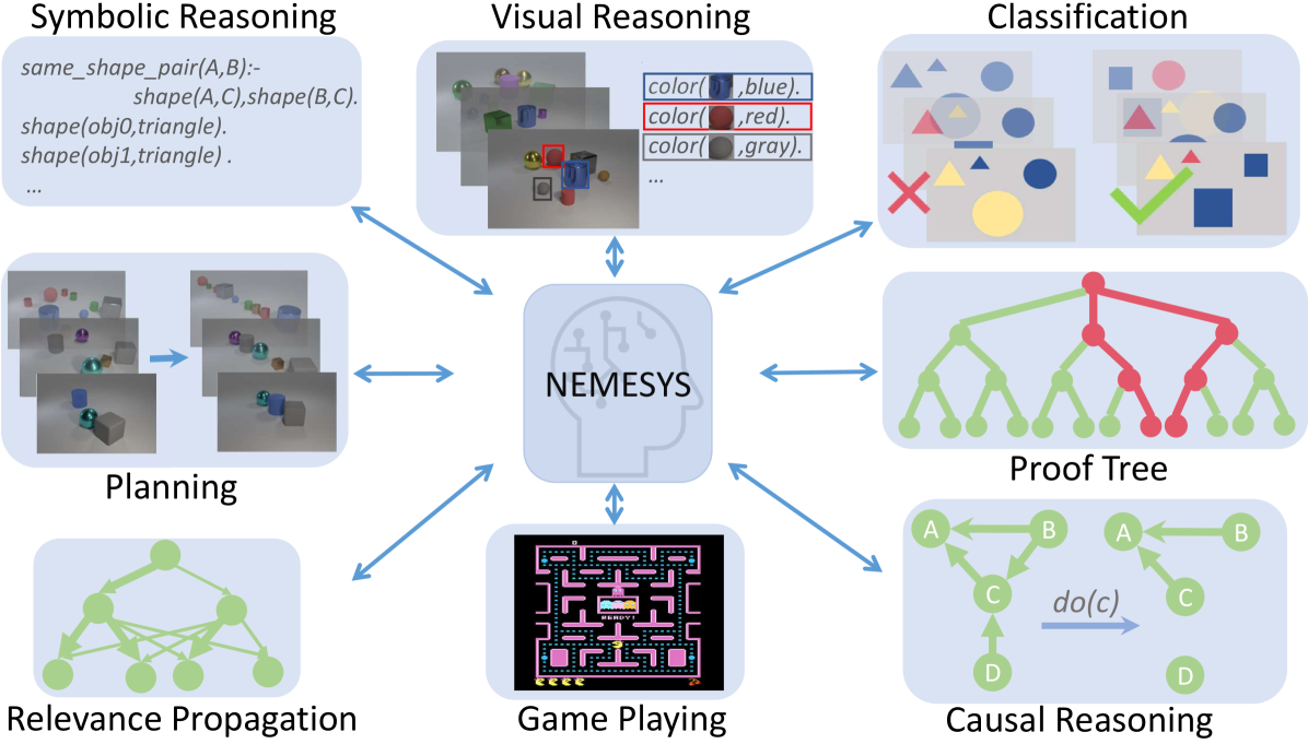
Figure 1: NEMESYS solves different kinds of tasks by using meta-level reasoning and learning. NEMESYS addresses, for instance, visual reasoning, planning, and causal reasoning without modifying its internal reasoning architecture. (Best viewed in color)
## 1 Introduction
One of the distant goals of Artificial Intelligence (AI) is to build a fully autonomous or ‘human-like’ system. The current successes of deep learning systems such as DALLE-2 [1], ChatGPT [2, 3], and Gato [4] have been promoted as bringing the field closer to this goal. However, current systems still require a large number of computations and often solve rather specific tasks. For example, DALLE-2 can generate very high-quality images but cannot play chess or Atari games. In stark contrast, human minds solve a wide range of problems using a small amount of computation and limited experience.
Most importantly, to be considered a major step towards achieving Artificial General Intelligence (AGI), a system must not only be able to perform a variety of tasks, such as Gato [4] playing Atari games, captioning images, chatting, and controlling a real robot arm, but also be self-reflective and able to learn and reason about its own capabilities. This means that it must be able to improve itself and adapt to new situations through self-reflection [5, 6, 7, 8]. Consequently, the study of meta-level architectures such as meta learning [9] and meta-reasoning [7] becomes progressively important. Meta learning [10] is a way to improve the learning algorithm itself [11, 12], i.e., it performs learning at a higher level, or meta-level. Meta-reasoning is a related concept that involves a system being able to think about its own abilities and how it processes information [5, 6]. It involves reflecting on, or introspecting about, the system’s own reasoning processes.
Indeed, meta-reasoning is different from object-centric reasoning, which refers to the system thinking about entities external to itself [13, 14, 15]. Here, the models perform low-level visual perception and reasoning on high-level concepts. Accordingly, there has been a push to make these reasoning systems differentiable [16, 17] along with addressing benchmarks in a visual domain such as CLEVR [18] and Kandinsky patterns [19, 20]. They use object-centric neural networks to perceive objects and perform reasoning using their output. Although this can solve the proposed benchmarks to some extent, the critical question remains unanswered: Is the reasoner able to justify its own operations? Can the same model solve different tasks such as (causal) reasoning, planning, game playing, and much more?
To overcome these limitations, we propose NEMESYS, the first neural meta -symbolic reasoning system. NEMESYS extensively performs meta-level programming on neuro-symbolic systems, and thus it can reason and learn several tasks. This is different from performing object-level deep reasoning and learning, which refers in some way to entities external to the system. NEMESYS is able to reflect or introspect, i.e., to shift from object- to meta-level reasoning and vice versa.
| | Meta Reasoning | Multitask Adaptation | Differentiable Meta Structure Learning |
| --- | --- | --- | --- |
| DeepProbLog [21] | ✗ | ✗ | ✗ |
| NTPs [22] | ✗ | ✗ | ✗ |
| FFSNL [23] | ✗ | ✗ | ✗ |
| $\alpha$ ILP [24] | ✗ | ✗ | ✗ |
| Scallop [25] | ✗ | ✗ | ✗ |
| NeurASP [26] | ✗ | ✗ | ✗ |
| NEMESYS (ours) | ✓ | ✓ | ✓ |
Table 1: Comparisons between NEMESYS and other state-of-the-art Neuro-Symbolic systems. We compare these systems with NEMESYS in three aspects, whether the system performs meta reasoning, can the same system adapt to solve different tasks and is the system capable of differentiable meta level structure learning.
Overall, we make the following contributions:
1. We propose NEMESYS, the first neural meta -symbolic reasoning and learning system that performs differentiable forward reasoning using meta-level programs.
1. To evaluate the ability of NEMESYS, we propose a challenging task, visual concept repairing, where the task is to rearrange objects in visual scenes based on relational logical concepts.
1. We empirically show that NEMESYS can efficiently solve different visual reasoning tasks with meta-level programs, achieving comparable performances with object-level forward reasoners [16, 24] that use specific programs for each task.
1. Moreover, we empirically show that using powerful differentiable meta-level programming, NEMESYS can solve different kinds of tasks that are difficult, if not impossible, for the previous neuro-symbolic systems. In our experiments, NEMESYS provides the function of (i) reasoning with integrated proof generation, i.e., performing differentiable reasoning producing proof trees, (ii) explainable artificial intelligence (XAI), i.e., highlighting the importance of logical atoms given conclusions, (iii) reasoning avoiding infinite loops, i.e., performing differentiable reasoning on programs which cause infinite loops that the previous logic reasoning systems unable to solve, and (iv) differentiable causal reasoning, i.e., performing causal reasoning [27, 28] on a causal Bayesian network using differentiable meta reasoners. To the best of the authors’ knowledge, we propose the first differentiable $\mathtt{do}$ operator. Achieving these functions with object-level reasoners necessitates significant efforts, and in some cases, it may be unattainable. In stark contrast, NEMESYS successfully realized the different useful functions by having different meta-level programs without any modifications of the reasoning function itself.
1. We demonstrate that NEMESYS can perform structure learning on the meta-level, i.e., learning meta programs from examples and adapting itself to solve different tasks automatically by learning efficiently with gradients.
To this end, we will proceed as follows. We first review (differentiable) first-order logic and reasoning. We then derive NEMESYS by introducing differentiable logical meta programming. Before concluding, we illustrate several capabilities of NEMESYS.
## 2 Background
NEMESYS relies on several research areas: first-order logic, logic programming, differentiable reasoning, meta-reasoning and -learning.
First-Order Logic (FOL)/Logic Programming. A term is a constant, a variable, or a term which consists of a function symbol. We denote $n$ -ary predicate ${\tt p}$ by ${\tt p}/(n,[{\tt dt_{1}},\ldots,{\tt dt_{n}}])$ , where ${\tt dt_{i}}$ is the datatype of $i$ -th argument. An atom is a formula ${\tt p(t_{1},\ldots,t_{n})}$ , where ${\tt p}$ is an $n$ -ary predicate symbol and ${\tt t_{1},\ldots,t_{n}}$ are terms. A ground atom or simply a fact is an atom with no variables. A literal is an atom or its negation. A positive literal is an atom. A negative literal is the negation of an atom. A clause is a finite disjunction ( $\lor$ ) of literals. A ground clause is a clause with no variables. A definite clause is a clause with exactly one positive literal. If $A,B_{1},\ldots,B_{n}$ are atoms, then $A\lor\lnot B_{1}\lor\ldots\lor\lnot B_{n}$ is a definite clause. We write definite clauses in the form of $A~{}\mbox{:-}~{}B_{1},\ldots,B_{n}$ . Atom $A$ is called the head, and a set of negative atoms $\{B_{1},\ldots,B_{n}\}$ is called the body. We call definite clauses as clauses for simplicity in this paper.
Differentiable Forward-Chaining Reasoning. The forward-chaining inference is a type of inference in first-order logic to compute logical entailment [29]. The differentiable forward-chaining inference [16, 17] computes the logical entailment in a differentiable manner using tensor-based operations. Many extensions of differentiable forward reasoners have been developed, e.g., reinforcement learning agents using logic to compute the policy function [30, 31] and differentiable rule learners in complex visual scenes [24]. NEMESYS performs differentiable meta-level logic programming based on differentiable forward reasoners.
<details>
<summary>x2.png Details</summary>
### Visual Description
## System Diagram: Differentiable Meta-Level Reasoning
### Overview
The image presents a system diagram illustrating differentiable meta-level reasoning, contrasted with object-level reasoning. It depicts the flow of information and processing steps involved in both approaches.
### Components/Axes
* **Titles:**
* "Differentiable Meta-Level Reasoning" (top)
* "Object-Level Reasoning" (bottom-left)
* "Meta Program" (bottom-right)
* **Nodes (Meta-Level Reasoning):**
* "clauses" (top-left)
* Contains the clause: `0.95:same_shape_pair(X,Y):- shape(X,Z), shape(Y,Z).`
* "Meta Converter" (top-center, pink)
* "meta probabilistic atoms" (top-center-right)
* Contains: `0.98:solve(shape(obj1, cube))`, `0.98:solve(shape(obj2, cube))`, `0.95:clause(same_shape_pair(obj1,obj2), (shape(obj1, cube), shape(obj2, cube)))`
* "Differentiable Forward Reasoner" (top-right, pink)
* "meta probabilistic atoms" (top-right)
* Contains: `0.98:solve(same_shape_pair(obj1,obj2))`
* **Nodes (Object-Level Reasoning):**
* "input" (bottom-left)
* Shows an image of three objects: a cyan cube, a red cube, and a yellow cylinder.
* "object-centric representation" (bottom-left)
* Shows a grid-based representation of the objects, with rows labeled "obj1", "obj2", and "obj3", and columns labeled "x" and "y". The grid cells are filled with blue squares, representing the object's presence at that location.
* Color legend: red circle, cyan circle, yellow circle, black square, 'o', 'x', 'y'
* "probabilistic atoms" (bottom-center)
* Contains: `0.98:color(obj1, cyan)`, `0.98:shape(obj1, cube)`, `0.98:color(obj2, red)`, `0.98:shape(obj2, cube)`
* **Nodes (Meta Program):**
* "naive interpreter" (bottom-right)
* Contains: `1.0:solve((A,B)):-solve(A), solve(B).`, `1.0:solve(A):-clause(A,B), solve(B).`
* "interpreter with proof trees" (bottom-right)
* Contains: `1.0:solve((A,B), (proofA, proofB)):-solve(A,proofA), solve(B, proofB).`, `1.0:solve(A, (A:-proofB)):-clause(A,B), solve(B, proofB).`
* **Arrows:** Arrows indicate the flow of information between the nodes.
### Detailed Analysis or ### Content Details
* **Meta-Level Reasoning Flow:**
1. "clauses" feeds into "Meta Converter".
2. "Meta Converter" outputs to "meta probabilistic atoms".
3. "meta probabilistic atoms" feeds into "Differentiable Forward Reasoner".
4. "Differentiable Forward Reasoner" outputs to "meta probabilistic atoms".
* **Object-Level Reasoning Flow:**
1. "input" feeds into "object-centric representation".
2. "object-centric representation" feeds into "probabilistic atoms".
* **Connection between Levels:**
* "probabilistic atoms" from Object-Level Reasoning feeds into "Meta Converter" in Meta-Level Reasoning.
### Key Observations
* The diagram illustrates a hierarchical reasoning process, where object-level information is abstracted and used for meta-level reasoning.
* Probabilistic atoms are used at both object and meta levels, indicating uncertainty in the reasoning process.
* The Meta Program provides different interpreters, one naive and one with proof trees, suggesting different levels of reasoning complexity.
### Interpretation
The diagram presents a system that combines object-level perception with meta-level reasoning. The object-level reasoning extracts features (color, shape, location) from the input image and represents them as probabilistic atoms. These atoms are then fed into the meta-level reasoning, which uses clauses and a forward reasoner to infer higher-level relationships and solve problems. The meta-program provides the logic for interpreting these relationships, with options for naive interpretation or more complex reasoning using proof trees. The system demonstrates a sophisticated approach to AI, where perception and reasoning are integrated to solve complex tasks.
</details>
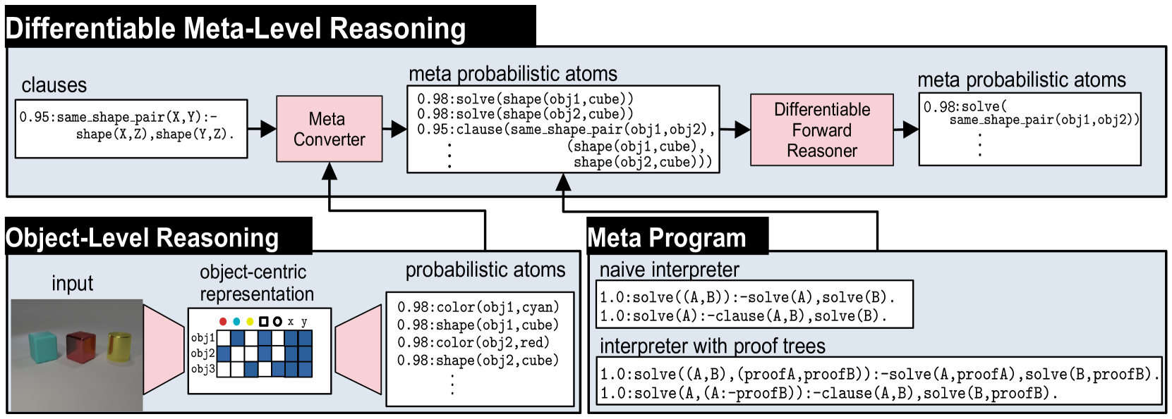
Figure 2: Overview of NEMESYS together with an object-level reasoning layer (bottom left). The meta-level reasoner (top) takes a logic program as input, here clauses on the left-hand side in the meta-level reasoning pipeline. Using the meta program (bottom right) it can realize the standard Prolog engine (naive interpreter) or an interpreter that provides e.g., also the proof trees (interpreter with proof trees) without requiring any alterations to the original logic program and internal reasoning function. This means that NEMESYS can integrate many useful functionalities by simply changing devised meta programs without intervening the internal reasoning function. (Best viewed in color)
Meta Reasoning and Learning. Meta-reasoning is the study about systems which are able to reason about its operation, i.e., a system capable of meta-reasoning may be able to reflect, or introspect [32], shifting from meta-reasoning to object-level reasoning and vice versa [6, 7]. Compared with imperative programming, it is relatively easier to construct a meta-interpreter using declarative programming. First-order Logic [33] has been the major tool to realize the meta-reasoning systems [34, 35, 36]. For example, Prolog [37] provides very efficient implementations of meta-interpreters realizing different additional features to the language.
Despite early interest in meta-reasoning within classical Inductive Logic Programming (ILP) systems [38, 39, 40], meta-interpreters have remained unexplored within neuro-symbolic AI. Meta-interpreters within classical logic are difficult to be combined with gradient-based machine learning paradigms, e.g., deep neural networks. NEMESYS realizes meta-level reasoning using differentiable forward reasoners in first-order logic, which are able to perform differentiable rule learning on complex visual scenes with deep neural networks [24]. Moreover, NEMESYS paves the way to integrate meta-level reasoning into other neuro-symbolic frameworks, including DeepProbLog [21], Scallop [25] and NeurASP [26], which are rather developed for training neural networks given logic programs using differentiable backward reasoning or answer set semantics. We compare NEMESYS with several popular neuro-symbolic systems in three aspects: whether the system performs meta reasoning, can the same system adapt to solve different tasks and is the system capable of differentiable meta level structure learning. The comparison results are summarized in Table 1.
## 3 Neural Meta-Symbolic Reasoning & Learning
We now introduce NEMESYS, the first neural meta-symbolic reasoning and learning framework. Fig. 2 shows an overview of NEMESYS.
### 3.1 Meta Logic Programming
We describe how meta-level programs are used in the NEMESYS workflow. In Fig. 2, the following object-level clause is given as its input:
| | $\displaystyle\mathtt{\color[rgb]{0,0.6,0}same\_shape\_pair(X,Y)\color[rgb]{ 0,0,0}\texttt{:-}\color[rgb]{0.68,0.36,1}shape(X,Z),shape(Y,Z)\color[rgb]{ 0,0,0}.}$ | |
| --- | --- | --- |
which identifies pairs of objects that have the same shape. The clause is subsequently fed to Meta Converter, which generates meta-level atoms.Using meta predicate $\mathtt{clause}/2$ , the following atom is generated:
| | $\displaystyle\mathtt{clause(\color[rgb]{0,0.6,0}same\_shape\_pair(X,Y),}\color [rgb]{0.68,0.36,1}\mathtt{(shape(X,Z),shape(Y,Z))\color[rgb]{0,0,0}).}$ | |
| --- | --- | --- |
where the meta atom $\mathtt{clause(H,B)}$ represents the object-level clause: $\mathtt{H\texttt{:-}B}$ .
To perform meta-level reasoning, NEMESYS uses meta-level programs, which often refer to meta interpreters, i.e., interpreters written in the language itself, as illustrated in Fig. 2. For example, a naive interpreter, NaiveInterpreter, is defined as:
| | $\displaystyle\mathtt{solve(true)}.$ | |
| --- | --- | --- |
To solve a compound goal $\mathtt{(A,B)}$ , we need first solve $\mathtt{A}$ and then $\mathtt{B}$ . A single goal $\mathtt{A}$ is solved if there is a clause that rewrites the goal to the new goal $\mathtt{B}$ , the body of the clause: $\mathtt{\color[rgb]{0,0.6,0}{A}\texttt{:-}\color[rgb]{0.68,0.36,1}{B}}$ . This process stops for facts, encoded as $\mathtt{clause(fact,true)}$ , since then, $\mathtt{solve(true)}$ will be true.
NEMESYS can employ more enriched meta programs with useful functions by simply changing the meta programs, without modifying the internal reasoning function, as illustrated in the bottom right of Fig. 2. ProofTreeInterpreter, an interpreter that produces proof trees along with reasoning, is defined as:
| | $\displaystyle\mathtt{solve(A,(A\texttt{:-}true)).}$ | |
| --- | --- | --- |
where $\mathtt{solve(A,Proof)}$ checks if atom $\mathtt{A}$ is true with proof tree $\mathtt{Proof}$ . Using this meta-program, NEMESYS can perform reasoning with integrated proof tree generation.
Now, let us devise the differentiable meta-level reasoning pipeline, which enables NEMESYS to reason and learn flexibly.
### 3.2 Differentiable Meta Programming
NEMESYS employs differentiable forward reasoning [24], which computes logical entailment using tensor operations in a differentiable manner, by adapting it to the meta-level atoms and clauses.
We define a meta-level reasoning function $f^{\mathit{reason}}_{(\mathcal{C},\mathbf{W})}:[0,1]^{G}\rightarrow[0,1]^{G}$ parameterized by meta-rules $\mathcal{C}$ and their weights $\mathbf{W}$ . We denote the set of meta-rules by $\mathcal{C}$ , and the set of all of the meta-ground atoms by $\mathcal{G}$ . $\mathcal{G}$ contains all of the meta-ground atoms produced by a given FOL language. We consider ordered sets here, i.e., each element has its index. We denote the size of the sets as: $G=|\mathcal{G}|$ and $C=|\mathcal{C}|$ . We denote the $i$ -th element of vector $\mathbf{x}$ by $\mathbf{x}[i]$ , and the $(i,j)$ -th element of matrix $\mathbf{X}$ by $\mathbf{X}[i,j]$ .
First, NEMESYS converts visual input to a valuation vector $\mathbf{v}\in[0,1]^{G}$ , which maps each meta atom to a probabilistic value (Fig. 2 Meta Converter). For example,
$$
\mathbf{v}=\blockarray{cl}\block{[c]l}0.98&\mathtt{solve(color(obj1,\ cyan))}
\\
0.01\mathtt{solve(color(obj1,\ red))}\\
0.95\mathtt{clause(same\_shape\_pair(\ldots),\ (shape(\ldots),\ \ldots))}\\
$$
represents a valuation vector that maps each meta-ground atom to a probabilistic value. For readability, only selected atoms are shown. NEMESYS computes logical entailment by updating the initial valuation vector $\mathbf{v}^{(0)}$ for $T$ times to $\mathbf{v}^{(T)}$ .
Subsequently, we compose the reasoning function that computes logical entailment. We now describe each step in detail.
(Step 1) Encode Logic Programs to Tensors.
To achieve differentiable forward reasoning, each meta-rule is encoded to a tensor representation. Let $S$ be the maximum number of substitutions for existentially quantified variables in $\mathcal{C}$ , and $L$ be the maximum length of the body of rules in $\mathcal{C}$ . Each meta-rule $C_{i}\in\mathcal{C}$ is encoded to a tensor ${\bf I}_{i}\in\mathbb{N}^{G\times S\times L}$ , which contains the indices of body atoms. Intuitively, $\mathbf{I}_{i}[j,k,l]$ is the index of the $l$ -th fact (subgoal) in the body of the $i$ -th rule to derive the $j$ -th fact with the $k$ -th substitution for existentially quantified variables. We obtain $\mathbf{I}_{i}$ by firstly grounding the meta rule $C_{i}$ , then computing the indices of the ground body atoms, and transforming them into a tensor.
(Step 2) Assign Meta-Rule Weights.
We assign weights to compose the reasoning function with several meta-rules as follows: (i) We fix the target programs’ size as $M$ , i.e., we try to select a meta-program with $M$ meta-rules out of $C$ candidate meta rules. (ii) We introduce $C$ -dimensional weights $\mathbf{W}=[{\bf w}_{1},\ldots,{\bf w}_{M}]$ where $\mathbf{w}_{i}\in\mathbb{R}^{C}$ . (iii) We take the softmax of each weight vector ${\bf w}_{j}\in\mathbf{W}$ and softly choose $M$ meta rules out of $C$ meta rules to compose the differentiable meta program.
(Step 3) Perform Differentiable Inference.
We compute $1$ -step forward reasoning using weighted meta-rules, then we recursively perform reasoning to compute $T$ -step reasoning.
(i) Reasoning using one rule. First, for each meta-rule $C_{i}\in\mathcal{C}$ , we evaluate body atoms for different grounding of $C_{i}$ by computing:
$$
\displaystyle b_{i,j,k}^{(t)}=\prod_{1\leq l\leq L}{\bf gather}({\bf v}^{(t)},
{\bf I}_{i})[j,k,l], \tag{1}
$$
where $\mathbf{gather}:[0,1]^{G}\times\mathbb{N}^{G\times S\times L}\rightarrow[0,1]^ {G\times S\times L}$ is:
$$
\displaystyle\mathbf{gather}({\bf x},{\bf Y})[j,k,l]={\bf x}[{\bf Y}[j,k,l]], \tag{2}
$$
and $b^{(t)}_{i,j,k}\in[0,1]$ . The $\mathbf{gather}$ function replaces the indices of the body atoms by the current valuation values in $\mathbf{v}^{(t)}$ . To take logical and across the subgoals in the body, we take the product across valuations. $b_{i,j,k}^{(t)}$ represents the valuation of body atoms for $i$ -th meta-rule using $k$ -th substitution for the existentially quantified variables to deduce $j$ -th meta-ground atom at time $t$ .
Now we take logical or softly to combine all of the different grounding for $C_{i}$ by computing $c^{(t)}_{i,j}\in[0,1]$ :
$$
\displaystyle c^{(t)}_{i,j}=\mathit{softor}^{\gamma}(b_{i,j,1}^{(t)},\ldots,b_
{i,j,S}^{(t)}), \tag{3}
$$
where $\mathit{softor}^{\gamma}$ is a smooth logical or function:
$$
\displaystyle\mathit{softor}^{\gamma}(x_{1},\ldots,x_{n})=\gamma\log\sum_{1
\leq i\leq n}\exp(x_{i}/\gamma), \tag{4}
$$
where $\gamma>0$ is a smooth parameter. Eq. 4 is an approximation of the max function over probabilistic values based on the log-sum-exp approach [41].
(ii) Combine results from different rules. Now we apply different meta-rules using the assigned weights by computing:
$$
\displaystyle h_{j,m}^{(t)}=\sum_{1\leq i\leq C}w^{*}_{m,i}\cdot c_{i,j}^{(t)}, \tag{5}
$$
where $h_{j,m}^{(t)}\in[0,1]$ , $w^{*}_{m,i}=\exp(w_{m,i})/{\sum_{i^{\prime}}\exp(w_{m,i^{\prime}})}$ , and $w_{m,i}=\mathbf{w}_{m}[i]$ . Note that $w^{*}_{m,i}$ is interpreted as a probability that meta-rule $C_{i}\in\mathcal{C}$ is the $m$ -th component. We complete the $1$ -step forward reasoning by combining the results from different weights:
$$
\displaystyle r_{j}^{(t)}=\mathit{softor}^{\gamma}(h_{j,1}^{(t)},\ldots,h_{j,M
}^{(t)}). \tag{6}
$$
Taking $\mathit{softor}^{\gamma}$ means that we compose $M$ softly chosen rules out of $C$ candidate meta-rules.
(iii) Multi-step reasoning. We perform $T$ -step forward reasoning by computing $r_{j}^{(t)}$ recursively for $T$ times: $v^{(t+1)}_{j}=\mathit{softor}^{\gamma}(r^{(t)}_{j},v^{(t)}_{j})$ . Updating the valuation vector for $T$ -times corresponds to computing logical entailment softly by $T$ -step forward reasoning. The whole reasoning computation Eq. 1 - 6 can be implemented using efficient tensor operations.
## 4 Experiments
With the methodology of NEMESYS established, we subsequently provide empirical evidence of its benefits over neural baselines and object-level neuro-symbolic approaches: (1) NEMESYS can emulate a differentiable forward reasoner, i.e., it is a sufficient implementation of object-centric reasoners with a naive meta program. (2) NEMESYS is capable of differentiable meta-level reasoning, i.e., it can integrate additional useful functions using devised meta-rules. We demonstrate this advantage by solving tasks of proof-tree generation, relevance propagation, automated planning, and causal reasoning. (3) NEMESYS can perform parameter and structure learning efficiently using gradient descent, i.e., it can perform learning on meta-level programs.
In our experiments, we implemented NEMESYS in Python using PyTorch, with CPU: intel i7-10750H and RAM: 16 GB.
| | NEMESYS | ResNet50 | YOLO+MLP |
| --- | --- | --- | --- |
| Twopairs | 100.0 $\bullet$ | 50.81 | 98.07 $\circ$ |
| Threepairs | 100.0 $\bullet$ | 51.65 | 91.27 $\circ$ |
| Closeby | 100.0 $\bullet$ | 54.53 | 91.40 $\circ$ |
| Red-Triangle | 95.6 $\bullet$ | 57.19 | 78.37 $\circ$ |
| Online/Pair | 100.0 $\bullet$ | 51.86 | 66.19 $\circ$ |
| 9-Circles | 95.2 $\bullet$ | 50.76 $\circ$ | 50.76 $\circ$ |
Table 2: Performance (accuracy; the higher, the better) on the test split of Kandinsky patterns. The best-performing models are denoted using $\bullet$ , and the runner-up using $\circ$ . In Kandinsky patterns, NEMESYS produced almost perfect accuracies outperforming neural baselines, where YOLO+MLP is a neural baseline using pre-trained YOLO [42] combined with a simple MLP, showing the capability of solving complex visual reasoning tasks. The performances of baselines are shown in [15].
### 4.1 Visual Reasoning on Complex Pattenrs
Let us start off by showing that our NEMESYS is able to obtain the equivalent high-quality results as a standard object-level reasoner but on the meta-level. We considered tasks of Kandinsky patterns [19, 43] and CLEVR-Hans [14] We refer to [14] and [15] for detailed explanations of the used patterns for CLEVR-Hans and Kandinsky patterns.. CLEVR-Hans is a classification task of complex 3D visual scenes. We compared NEMESYS with the naive interpreter against neural baselines and a neuro-symbolic baseline, $\alpha$ ILP [24], which achieves state-of-the-art performance on these tasks. For all tasks, NEMESYS achieved exactly the same performances with $\alpha$ ILP since the naive interpreter realizes a conventional object-centric reasoner. Moreover, as shown in Table 2 and Table 3, NEMESYS outperformed neural baselines on each task. This shows that NEMESYS is able to solve complex visual reasoning tasks using meta-level reasoning without sacrificing performance.
In contrast to the object-centric reasoners, e.g., $\alpha$ ILP. NEMESYS can easily integrate additional useful functions by simply switching or adding meta programs without modifying the internal reasoning function, as shown in the next experiments.
### 4.2 Explainable Logical Reasoning
One of the major limitations of differentiable forward chaining [16, 17, 24] is that they lack the ability to explain the reasoning steps and their evidence. We show that NEMESYS achieves explainable reasoning by incorporating devised meta-level programs.
Reasoning with Integrated Proof Tree Generation
First, we demonstrate that NEMESYS can generate proof trees while performing reasoning, which the previous differentiable forward reasoners cannot produce since they encode the reasoning function to computational graphs using tensor operations and observe only their input and output. Since NEMESYS performs reasoning using meta-level programs, it can add the function to produce proof trees into its underlying reasoning mechanism simply by devising them, as illustrated in Fig 2.
We use Kandinsky patterns [20], a benchmark of visual reasoning whose classification rule is defined on high-level concepts of relations and attributes of objects. We illustrate the input on the top right of Fig. 3 that belongs to a pattern: ”There are two pairs of objects that share the same shape.” Given the visual input, proof trees generated using the ProofTreeInterpreter in Sec. 3.1 are shown on the left two boxes of Fig. 3. In this experiment, NEMESYS identified the relations between objects, and the generated proof trees explain the intermediate reasoning steps.
<details>
<summary>x3.png Details</summary>
### Visual Description
## Diagram: Relevance Proof Propagation
### Overview
The image presents a diagram illustrating relevance proof propagation, alongside proof trees. It shows how the system determines the similarity of shapes between objects, using a tree-like structure to represent the propagation of evidence.
### Components/Axes
* **Titles:**
* "Proof Trees" (top-left)
* "Relevance Proof Propagation" (top-right)
* **Objects:**
* obj0 (blue triangle)
* obj1 (blue square)
* obj2 (red triangle)
* obj3 (blue square)
* **Nodes:** The diagram uses rounded rectangles to represent nodes, with text indicating the function or relationship being evaluated.
* **Edges:** Green lines connect the nodes, indicating the flow of information or relevance. The thickness of the lines varies, suggesting different levels of relevance or confidence.
* **Shapes:** Triangle (△), Square (□)
### Detailed Analysis
**1. Proof Trees (Left Side):**
* **Top Tree (Blue Background):**
* Confidence: 0.98
* Function: `same_shape_pair(obj0, obj2)`
* Sub-functions:
* `(0.98 shape(obj0, △):- true)`
* `(0.98 shape(obj2, △):- true)`
* **Bottom Tree (Orange Background):**
* Confidence: 0.02
* Function: `same_shape_pair(obj0, obj1)`
* Sub-functions:
* `(0.98 shape(obj0, △):- true)`
* `(0.02 shape(obj1, △):- true)`
**2. Relevance Proof Propagation (Right Side):**
* **Top Section (Gray Background):**
* Contains shapes representing objects:
* obj0: Blue Triangle
* obj1: Blue Square
* obj2: Red Triangle
* obj3: Blue Square
* **Middle Layer:**
* Node 1: `same_shape_pair(△, △)` (connected to obj0 and obj2)
* Node 2: `same_shape_pair(△, □)` (connected to obj0 and obj1)
* **Bottom Layer:**
* Node 1: `0.96 shape(△, △)` (connected to `same_shape_pair(△, △)`)
* Node 2: `0.96 shape(△, △)` (connected to `same_shape_pair(△, △)`)
* Node 3: `0.1 shape(□, △)` (connected to `same_shape_pair(△, □)`)
**3. Edge Connections:**
* The green lines connect the objects in the gray box to the `same_shape_pair` nodes.
* The `same_shape_pair` nodes are connected to the `shape` nodes in the bottom layer.
* The thickness of the lines varies, indicating the strength of the relationship or relevance.
### Key Observations
* The proof trees on the left provide the logical rules and confidence scores for determining shape similarity.
* The relevance proof propagation diagram on the right visually represents how these rules are applied to specific objects.
* The confidence scores (0.98, 0.02, 0.96, 0.1) indicate the certainty of the shape relationships.
* The varying thickness of the lines suggests different levels of relevance or confidence in the connections.
### Interpretation
The diagram illustrates a system for determining the relevance of shape relationships between objects. The proof trees define the rules and confidence scores, while the relevance proof propagation diagram shows how these rules are applied to specific objects. The system appears to be evaluating whether objects have the same shape (triangle or square) and assigning a confidence score to each relationship. The higher the confidence score, the more likely the objects are to have the same shape. The varying thickness of the lines suggests that some relationships are more relevant or have a higher degree of confidence than others. The diagram highlights the process of reasoning and evidence propagation in determining object similarity.
</details>
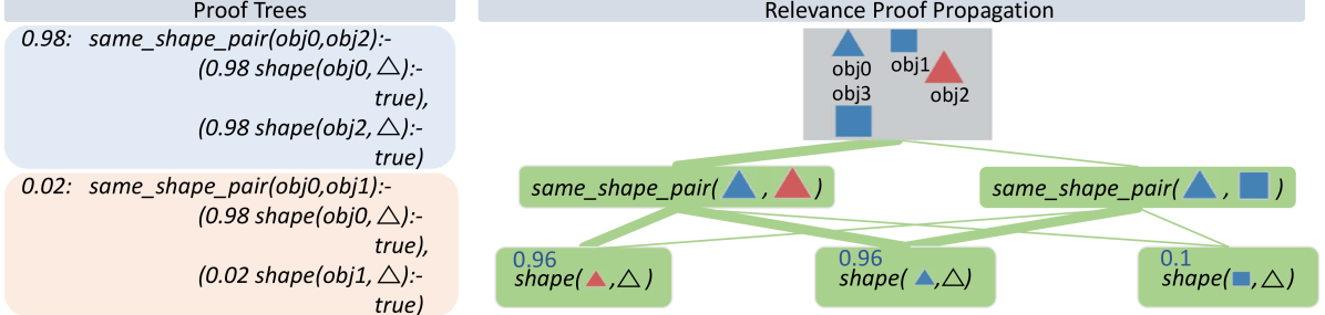
Figure 3: NEMESYS explains its reasoning with proof trees and relevance proof propagation. Given the image involving four objects (top, right), NEMESYS provides two proofs (two boxes on the left, true atom’s proof (blue box) and false atom’s proof (cream box)). They can be leveraged to decompose the prediction of NEMESYS into relevance scores per (ground) atom (right). First, a standard forward reasoning is performed to compute the prediction. Then, the model’s prediction is backward propagated through the proof trees by applying specific decomposition rules, see main text. The numbers next to each (ground) atom are the relevance scores computed. The larger the score is, the more impact an (ground) atom has on the final prediction, and the line width is wider. For brevity, the complete proof tree is not depicted here. As our baseline comparison, we extend DeepProbLog [21] to DeepMetaProbLog. However, DeepMetaProbLog only provides proof tree for true atoms (top left blue box). (Best viewed in color)
| | CLEVR-Hans3 | CLEVR-Hans7 | | |
| --- | --- | --- | --- | --- |
| Validation | Test | Validation | Test | |
| CNN | 99.55 $\circ$ | 70.34 | 96.09 | 84.50 |
| NeSy (Default) | 98.55 | 81.71 | 96.88 $\circ$ | 90.97 |
| NeSy-XIL | 100.00 $\bullet$ | 91.31 $\circ$ | 98.76 $\bullet$ | 94.96 $\bullet$ |
| NEMESYS | 98.18 | 98.40 $\bullet$ | 93.60 | 92.19 $\circ$ |
Table 3: Performance (accuracy; the higher, the better) on the validation/test splits of 3D CLEVR-Hans data sets. The best-performing models are denoted using $\bullet$ , and the runner-up using $\circ$ . In CLEVR-Hans, NEMESYS outperformed neural baselines including: (CNN) A ResNet [44], (NeSy) A model combining object-centric model (Slot Attention [45] and Set Transformer [46], and (NeSy-XIL) Slot Attention and Set Transformer using human feedback. NEMESYS tends to show less overfitting and performs similarly to a neuro-symbolic approach using human feedback (NeSy-XIL). The performances of baselines are shown in [14] and [15].
Let’s first consider the top left blue box depicted in Fig. 3 (for readability, we only show the proof part of meta atoms in the image). The weighted ground atom $\mathtt{0.98:}\mathtt{same\_shape\_pair(obj0,obj2)}$ proves $\mathtt{obj0}$ and $\mathtt{obj2}$ are of the same shape with the probability $0.98$ . The proof part shows that NEMESYS comes to this conclusion since both objects are triangle with probabilities of $\mathtt{0.98}$ and in turn it can apply the rule for $\mathtt{same\_shape\_pair}$ . We use this example to show how to compute the weight of the meta atoms inside NEMESYS. With the proof-tree meta rules and corresponding meta ground atoms:
| | $\displaystyle\mathtt{0.98:}\ \color[rgb]{0.5,0,1}\mathtt{solve(shape(obj0,} \text{\includegraphics[height=6.45831pt]{plots/triangle.png}}\mathtt{),(shape( obj0,}\text{\includegraphics[height=6.45831pt]{plots/triangle.png}}\mathtt{), true).}$ | |
| --- | --- | --- |
The weight of the meta ground atoms are computed by Meta Converter when mapping the probability of meta ground atoms to a continuous value. The meta ground atom says that $\mathtt{shape(obj0,\includegraphics[height=6.45831pt]{plots/triangle.png})}$ is true with a high probability of $0.98$ because $\mathtt{shape(obj0,\includegraphics[height=6.45831pt]{plots/triangle.png})}$ can be proven.
With the two meta ground atoms at hand, we infer the weight of the meta atom with compound goals $\color[rgb]{0,0.6,0}\mathtt{solve((shape(obj0,\includegraphics[height=6.45831 pt]{plots/triangle.png}),shape(obj2,\includegraphics[height=6.45831pt]{plots/ triangle.png})),(ProofA,ProofB))}$ , based on the first meta rule (for readability, we omit writing out the proof part). Then, we use the second meta rule to compute the weight of the meta atom $\color[rgb]{0.68,0.36,1}\mathtt{solve}\mathtt{(same\_shape\_pair(obj0,obj2)}, \mathtt{(Proof))}$ , using the compound goal meta atom $\color[rgb]{0,0.6,0}\mathtt{solve((shape(obj0,\includegraphics[height=6.45831 pt]{plots/triangle.png}),shape(obj2,\includegraphics[height=6.45831pt]{plots/ triangle.png})),(ProofA,ProofB))}$ and the meta atom $\mathtt{clause}\mathtt{(same\_shape\_pair(obj0,obj2)},\mathtt{(shape(obj0, \includegraphics[height=6.45831pt]{plots/triangle.png})},\mathtt{shape(obj2, \includegraphics[height=6.45831pt]{plots/triangle.png})))}$ .
In contrast, NEMESYS can explicitly show that $\mathtt{obj0}$ and $\mathtt{obj1}$ have a low probability of being of the same shape (Fig. 3 left bottom cream box). This proof tree shows that the goal $\mathtt{shape(obj1,\includegraphics[height=6.45831pt]{plots/triangle.png})}$ has a low probability of being true. Thus, as one can read off, $\mathtt{obj0}$ is most likely a triangle, while $\mathtt{obj1}$ is most likely not a triangle. In turn, NEMESYS concludes with a low probability that $\mathtt{same\_shape\_pair(obj0,obj1)}$ is true, only a probability of $0.02$ . NEMESYS can produce all the information required to explain its decisions by simply changing the meta-program, not the underlying reasoning system.
Using meta programming to extend DeepProbLog to produce proof trees as a baseline comparison. Since DeepProbLog [21] doesn’t support generating proof trees in parallel with reasoning, we extend DeepProbLog [21] to DeepMetaProblog to generate proof trees as our baseline comparison using ProbLog [47]. However, the proof tree generated by DeepMetaProbLog is limited to the ‘true’ atoms (Fig. 3 top left blue box), i.e., DeepMetaProbLog is unable to generate proof tree for false atoms such as $\mathtt{same\_shape\_pair(obj0,obj1)}$ (Fig. 3 bottom left cream box) due to backward reasoning.
Logical Relevance Proof Propagation (LRP ${}^{2}$ )
Inspired by layer-wise relevance propagation (LRP) [48], which produces explanations for feed-forward neural networks, we now show that, LRP can be adapted to logical reasoning systems using declarative languages in NEMESYS, thereby enabling the reasoning system to articulate the rationale behind its decisions, i.e., it can compute the importance of ground atoms for a query by having access to proof trees. We call this process: logical relevance proof propagation (LRP ${}^{2}$ ).
The original LRP technique decomposes the prediction of the network, $f(\mathbf{x})$ , onto the input variables, $\mathbf{x}=\left(x_{1},\ldots,x_{d}\right)$ , through a decomposition $\mathbf{R}=\left(R_{1},\ldots,R_{d}\right)$ such that $\sum\nolimits_{p=1}^{d}R_{p}=f(\mathbf{x})\;$ . Given the activation $a_{j}=\rho\left(\sum_{i}a_{i}w_{ij}+b_{j}\right)$ of neuron, where $i$ and $j$ denote the neuron indices at consecutive layers, and $\sum_{i}$ and $\sum_{j}$ represent the summation over all neurons in the respective layers, the propagation of LRP is defined as: $R_{i}=\sum\nolimits_{j}z_{ij}({\sum\nolimits_{i}z_{ij}})^{-1}R_{j},$ where $z_{ij}$ is the contribution of neuron $i$ to the activation $a_{j}$ , typically some function of activation $a_{i}$ and the weight $w_{ij}$ . Starting from the output $f(\mathbf{x})$ , the relevance is computed layer by layer until the input variables are reached.
To adapt this in NEMESYS to ground atoms and proof trees, we have to be a bit careful, since we cannot deal with the uncountable, infinite real numbers within our logic. Fortunately, we can make use of the weight associated with ground atoms. That is, our LRP ${}^{2}$ composes meta-level atoms that represent the relevance of an atom given proof trees and associates the relevance scores to the weights of the meta-level atoms.
To this end, we introduce three meta predicates: $\mathtt{rp/3/[goal,proofs,atom]}$ that represents the relevance score an $\mathtt{atom}$ has on the $\mathtt{goal}$ in given $\mathtt{proofs}$ , $\mathtt{assert\_probs/1/[atom]}$ that looks up the valuations of the ground atoms and maps the probability of the $\mathtt{atom}$ to its weight. $\mathtt{rpf/2/[proof,atom]}$ represents how much an $\mathtt{atom}$ contributes to the $\mathtt{proof}$ . The atom $\mathtt{assert\_probs((Goal\texttt{:-}Body))}$ asserts the probability of the atom $\mathtt{(Goal\texttt{:-}Body)}$ . With them, the meta-level program of LRP ${}^{2}$ is:
| | $\displaystyle\mathtt{rp(Goal,Body,Atom)}\texttt{:-}\mathtt{assert\_probs((Goal \texttt{:-}Body))},$ | |
| --- | --- | --- |
where $\mathtt{rp(Goal,Proof,Atom)}$ represents the relevance score an $\mathtt{Atom}$ has on the $\mathtt{Goal}$ in a $\mathtt{Proof}$ , i.e., we interpret the associated weight with atom $\mathtt{rp(Goal,Proof,Atom)}$ as the actual relevance score of $\mathtt{Atom}$ has on $\mathtt{Goal}$ given $\mathtt{Proof}$ . The higher the weight of $\mathtt{rp(Goal,Proof,Atom)}$ is, the larger the impact of $\mathtt{Atom}$ has on the $\mathtt{Goal}$ .
Let us go through the meta rules of LRP ${}^{2}$ . The first rule defines how to compute the relevance score of an $\mathtt{Atom}$ given the $\mathtt{Goal}$ under the condition of a $\mathtt{Body}$ (a single $\mathtt{Proof}$ ). The relevance score is computed by multiplying the weight of the $\mathtt{Body}$ , the weight of a clause $\mathtt{(Goal\texttt{:-}Body)}$ and the importance score of the $\mathtt{Atom}$ given the $\mathtt{Body}$ . The second to the seventh rule defines how to calculate the importance score of an $\mathtt{Atom}$ given a $\mathtt{Proof}$ . These six rules loop over each atom of the given $\mathtt{Proof}$ , once it detects the $\mathtt{Atom}$ inside the given $\mathtt{Proof}$ , the importance score will be set to the weight of the $\mathtt{Atom}$ , another case is that the $\mathtt{Atom}$ is not in $\mathtt{Proof}$ , in that case, in the seventh rule, $\mathtt{norelate}$ will set the importance score to a small value. The eighth and ninth rules amalgamate the results from different proofs, i.e., the score from each proof tree is computed recursively during forward reasoning. The scores for the same target (the pair of $\mathtt{Atom}$ and $\mathtt{Goal}$ ) are combined by the $\mathit{softor}$ operation. The score of an atom given several proofs is computed by taking logical or softly over scores from each proof.
With these nine meta rules at hand, together with the proof tree, NEMESYS is able to perform the relevance proof propagation for different atoms. We consider using the proof tree generated in Sec. 4.2 and set the goal as: $\mathtt{same\_shape\_pair(obj0,obj2)}$ . Fig. 3 (right) shows LRP ${}^{2}$ -based explanations generated by NEMESYS. The relevance scores of different ground atoms are listed next to each (ground) atom. As we can see, the atoms $\mathtt{shape(obj0,\includegraphics[height=6.45831pt]{plots/triangle.png})}$ and $\mathtt{shape(obj2,\includegraphics[height=6.45831pt]{plots/triangle.png})}$ have the largest impact on the goal $\mathtt{same\_shape\_pair(obj0,obj2)}$ , while $\mathtt{shape(obj1,\includegraphics[height=6.45831pt]{plots/triangle.png})}$ have much smaller impact.
By providing proof tree and LRP ${}^{2}$ , NEMESYS computes the precise effect of a ground atom on the goal and produces an accurate proof to support its conclusion. This approach is distinct from the Most Probable Explanation (MPE) [49], which generates the most probable proof rather than the exact proof.
<details>
<summary>extracted/5298395/images/plan/0v.png Details</summary>
### Visual Description
## Still Life: Geometric Shapes
### Overview
The image is a still life featuring three geometric shapes: a large purple sphere, a smaller metallic purple sphere, and a red cylinder. The shapes are arranged on a light gray surface with a gradient background.
### Components/Axes
* **Shapes:**
* Large Sphere: Located towards the top-center of the image, matte purple color.
* Small Sphere: Located to the left of the large sphere, metallic purple color.
* Cylinder: Located to the right of the large sphere, red color.
* **Surface:** Light gray, appears to be a flat plane.
* **Background:** Gradient from light gray to darker gray, suggesting a light source from the left.
### Detailed Analysis or ### Content Details
* **Large Sphere:** Positioned slightly above the center of the image. The diameter of the sphere is approximately 1/5 of the image width.
* **Small Sphere:** Positioned to the left and slightly below the large sphere. It has a reflective surface. The diameter of the sphere is approximately 1/10 of the image width.
* **Cylinder:** Positioned to the right and slightly below the large sphere. The height of the cylinder is approximately 1/15 of the image width, and the diameter is similar.
* **Lighting:** The lighting creates soft shadows behind each object, indicating a diffused light source.
### Key Observations
* The arrangement of the shapes is asymmetrical, with the large sphere acting as a central point.
* The contrast in color and texture between the matte purple sphere, the metallic purple sphere, and the red cylinder adds visual interest.
* The gradient background provides depth to the image.
### Interpretation
The image is a simple composition that highlights the basic geometric forms and their interaction with light and shadow. The arrangement of the shapes and the use of color create a visually balanced and aesthetically pleasing image. The image does not provide any specific data or facts beyond the visual representation of the shapes.
</details>
<details>
<summary>extracted/5298395/images/plan/1v0.png Details</summary>
### Visual Description
## Still Life: Geometric Shapes
### Overview
The image is a still life featuring three geometric shapes: a large purple sphere, a smaller metallic purple sphere, and a red cylinder. They are arranged on a light gray surface with a gradient background.
### Components/Axes
* **Shapes:**
* Large Purple Sphere: Located towards the top-left of the image.
* Small Metallic Purple Sphere: Positioned below and slightly to the right of the large sphere.
* Red Cylinder: Situated to the right of the small sphere.
* **Surface:** Light gray with a subtle gradient.
* **Background:** Light gray, slightly darker than the surface.
### Detailed Analysis
* **Large Purple Sphere:** The sphere has a matte finish and is a solid purple color.
* **Small Metallic Purple Sphere:** This sphere has a reflective, metallic surface, with highlights and shadows indicating its roundness.
* **Red Cylinder:** The cylinder is a solid red color with a flat top and bottom.
* **Arrangement:** The shapes are arranged in a loose triangular formation. The large sphere is the highest, followed by the small sphere, and then the cylinder.
* **Lighting:** The lighting appears to be coming from the left, casting shadows to the right of each object.
### Key Observations
* The contrast between the matte and metallic surfaces of the spheres is notable.
* The color palette is limited to purple and red, creating a simple and visually appealing composition.
* The arrangement of the shapes creates a sense of depth and perspective.
### Interpretation
The image is a study in form, color, and texture. The simple geometric shapes are arranged in a way that is both visually pleasing and thought-provoking. The contrast between the matte and metallic surfaces, as well as the limited color palette, creates a sense of harmony and balance. The image could be interpreted as a representation of simplicity, order, and beauty.
</details>
<details>
<summary>extracted/5298395/images/plan/1v1.png Details</summary>
### Visual Description
## Geometric Shapes Arrangement
### Overview
The image depicts three geometric shapes - a large purple sphere, a smaller metallic purple sphere, and a red cylinder - arranged on a light gray surface. The lighting appears to originate from the top-left, casting shadows behind the objects.
### Components/Axes
* **Shapes:**
* Large Sphere: Located towards the top-left, colored purple.
* Small Sphere: Located between the large sphere and the cylinder, colored metallic purple.
* Cylinder: Located towards the bottom-right, colored red.
* **Surface:** Light gray, acting as the background.
* **Lighting:** Appears to be coming from the top-left, creating shadows behind the shapes.
### Detailed Analysis or ### Content Details
* **Large Purple Sphere:** Positioned in the upper-left quadrant of the image. It is a matte purple color.
* **Small Metallic Purple Sphere:** Positioned to the right and slightly below the large sphere. It has a reflective, metallic surface.
* **Red Cylinder:** Positioned to the right and slightly below the small sphere. It appears to be a solid red color.
* **Shadows:** Each shape casts a shadow, indicating a light source from the top-left. The shadows are darker closer to the base of the shapes and fade as they extend away.
### Key Observations
* The shapes are arranged in a diagonal line from the top-left to the bottom-right.
* The size of the spheres decreases from left to right.
* The cylinder is the only non-spherical shape.
* The lighting highlights the different surface properties of the shapes (matte vs. metallic).
### Interpretation
The image appears to be a simple composition of geometric shapes, possibly for illustrative or demonstrative purposes. The arrangement and lighting create a sense of depth and visual interest. The different colors and surface properties of the shapes add to the overall aesthetic. The image does not provide any specific data or facts beyond the visual representation of the shapes and their arrangement.
</details>
<details>
<summary>extracted/5298395/images/plan/final.png Details</summary>
### Visual Description
## Geometric Shapes: Simple Scene
### Overview
The image depicts a simple scene with three geometric shapes: a large purple sphere, a smaller metallic purple sphere, and a red cylinder. They are arranged on a light gray surface with subtle shadows, suggesting a rendered or simulated environment.
### Components/Axes
* **Shapes:**
* Large Sphere: Located on the left side of the image, matte purple color.
* Small Sphere: Located to the right of the large sphere, metallic purple color.
* Cylinder: Located on the right side of the image, red color.
* **Surface:** Light gray, providing a neutral background.
* **Lighting:** Appears to be a single light source, casting shadows behind the shapes.
### Detailed Analysis or ### Content Details
* **Large Sphere:** Positioned in the top-left quadrant of the image. The color is a matte purple.
* **Small Sphere:** Positioned to the right and slightly below the large sphere. The color is a metallic purple, reflecting light.
* **Cylinder:** Positioned on the right side of the image, slightly below the small sphere. The color is red.
* **Shadows:** Each shape casts a shadow, indicating a light source from the top-left. The shadows are soft and diffuse.
### Key Observations
* The arrangement of the shapes is simple and uncluttered.
* The color palette is limited to purple, red, and gray.
* The lighting is soft and even, creating a sense of depth.
### Interpretation
The image appears to be a basic 3D rendering or a simple composition of geometric shapes. The arrangement and lighting suggest a deliberate attempt to create a visually pleasing scene. The use of different materials (matte vs. metallic) adds visual interest. There is no explicit data or information being conveyed beyond the visual representation of the shapes and their arrangement.
</details>
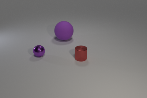
Figure 4: Visual Concept Repairing: NEMESYS achieves planning by performing differentiable meta-level reasoning. The left most image shows the start state, and the right most image shows the goal state. Taking these states as inputs, NEMESYS performs differentiable forward reasoning using meta-level clauses that simulate the planning steps and generate intermediate states (two images in the middle) and actions from start state to reach the goal state. (Best viewed in color)
### 4.3 Avoiding Infinite Loops
Differentiable forward chaining [17], unfortunately, can generate infinite computations. A pathological example:
| | $\displaystyle\mathtt{edge(a,b).\ edge(b,a).}\ \mathtt{edge(b,c).}\quad\mathtt{ path(A,A,[\ ]).}\quad$ | |
| --- | --- | --- |
<details>
<summary>x4.png Details</summary>
### Visual Description
## Bar Chart: Accuracy Test on 4 Queries
### Overview
The image is a bar chart comparing the accuracy of two systems, ProbLog and NEMESYS, based on a test of 4 queries. The y-axis represents accuracy, ranging from 0.0 to 1.0. The x-axis represents the two systems being compared.
### Components/Axes
* **Title:** Test on 4 queries
* **X-axis:**
* Labels: ProbLog, NEMESYS
* **Y-axis:**
* Label: Accuracy
* Scale: 0.0, 0.5, 1.0
* **Bars:**
* ProbLog: Light blue/purple color
* NEMESYS: Light red/orange color
### Detailed Analysis
* **ProbLog:** The light blue/purple bar reaches an accuracy of approximately 0.75.
* **NEMESYS:** The light red/orange bar reaches an accuracy of 1.0.
### Key Observations
* NEMESYS achieves a higher accuracy (1.0) compared to ProbLog (0.75) on the test of 4 queries.
### Interpretation
The bar chart indicates that NEMESYS outperforms ProbLog in terms of accuracy when tested on the given 4 queries. NEMESYS achieves perfect accuracy, while ProbLog's accuracy is at 75%. This suggests that, for these specific queries, NEMESYS is a more reliable system. The limited number of queries (4) should be considered when generalizing these results.
</details>
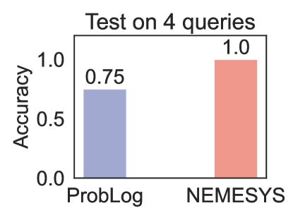
Figure 5: Performance (accuracy; the higher, the better)on four queries. (Best viewed in color)
It defines a simple graph over three nodes $(a,b,c)$ with three edges, $(a-b,b-a,b-c)$ as well as paths in graphs in general. Specifically, $\mathtt{path}/3$ defines how to find a path between two nodes in a recursive way. The base case is $\mathtt{path(A,A,[])}$ , meaning that any node $\mathtt{A}$ is reachable from itself. The recursion then says, if there is an edge from node $\mathtt{A}$ to node $\mathtt{B}$ , and there is a path from node $\mathtt{B}$ to node $\mathtt{C}$ , then there is a path from node $\mathtt{A}$ to node $\mathtt{C}$ . Unfortunately, this generates an infinite loop $\mathtt{[edge(a,b),edge(b,a),edge(a,b),\ldots]}$ when computing the path from $a$ to $c$ , since this path can always be extended potentially also leading to the node $c$ .
Fortunately, NEMESYS allows one to avoid infinite loops by memorizing the proof-depth, i.e., we simply implement a limited proof-depth strategy on the meta-level:
| | $\displaystyle\mathtt{li((A,B),DPT)}\texttt{:-}\mathtt{li(A,DPT)},\mathtt{li(B, DPT).}$ | |
| --- | --- | --- |
With this proof strategy, NEMESYS gets the path $\mathtt{path(a,c,[edge(a,b),edge(b,c)])=true}$ in three steps. For simplicity, we omit the proof part in the atom. Using the second rule and the first rule recursively, the meta interpreter finds $\mathtt{clause(path(a,c),(edge(a,b),path(b,c)))}$ and $\mathtt{clause(path(b,c),(edge(b,c),path(c,c)))}$ . Finally, the meta interpreter finds a clause, whose head is $\mathtt{li(path(c,c),1)}$ and the body is true.
Since forward chaining gets stuck in the infinite loop, we choose ProbLog [47] as our baseline comparison. We test NEMESYS and ProbLog using four queries, including one query which calls the recursive rule. ProbLog fails to return the correct answer on the query which calls the recursive rule. The comparison is summarized in Fig. 5. We provide the four test queries in Appendix A.
### 4.4 Differentiable First-Order Logical Planning
As the fourth meta interpreter, we demonstrate NEMESYS as a differentiable planner. Consider Fig. 4 where NEMESYS was asked to put all objects of a start image onto a line. Each start and goal state is represented as a visual scene, which is generated in the CLEVR [18] environment. By adopting a perception model, e.g., YOLO [42] or slot attention [45], NEMESYS obtains logical representations of the start and end states:
| | $\displaystyle\mathtt{start}$ | $\displaystyle=\{\mathtt{pos(obj0,(1,3)),\ldots,pos(obj4,(2,1))}\},$ | |
| --- | --- | --- | --- |
where $\mathtt{pos/2}$ describes the $2$ -dim positions of objects. NEMESYS solves this planning task by performing differentiable reasoning using the meta-level program:
| | $\displaystyle\mathtt{plan(Start\_state,}\mathtt{New\_state,Goal\_state,[Action ,Old\_stack])}\textbf{:-}$ | |
| --- | --- | --- |
The first meta rule presents the recursive rule for plan generation, and the second rule gives the successful termination condition for the plan when the $\mathtt{Goal\_state}$ is reached, where $\mathtt{equal/2}$ checks whether the $\mathtt{Current\_state}$ is the $\mathtt{Goal\_state}$ and the $\mathtt{planf/3}$ contains $\mathtt{Start\_state}$ , $\mathtt{Goal\_state}$ and the needed action sequences $\mathtt{Move\_stack}$ from $\mathtt{Start\_state}$ to reach the $\mathtt{Goal\_state}$ .
The predicate $\mathtt{plan/4}$ takes four entries as inputs: $\mathtt{Start\_state}$ , $\mathtt{State}$ , $\mathtt{Goal\_state}$ and $\mathtt{Move\_stack}$ . The $\mathtt{move/3}$ predicate uses $\mathtt{Action}$ to push $\mathtt{Old\_state}$ to $\mathtt{New\_state}$ . $\mathtt{condition\_met/2}$ checks if the state’s preconditions are met. When the preconditions are met, $\mathtt{change\_state/2}$ changes the state, and $\mathtt{plan/4}$ continues the recursive search.
To reduce memory usage, we split the move action in horizontal and vertical in the experiment. For example, NEMESYS represents an action to move an object in the horizontal direction right by $\mathtt{1}$ step using meta-level atom:
| | $\displaystyle\mathtt{move(}$ | $\displaystyle\mathtt{move\_right},\mathtt{pos\_hori(Object,X),}\mathtt{pos\_ hori(Object,X}\texttt{+}\mathtt{1)).}$ | |
| --- | --- | --- | --- |
where $\mathtt{move\_right}$ represents the action, $\mathtt{X+1}$ represents arithmetic sums over (positive) integers, encoded as $\mathtt{0,succ(0),succ(succ(0))}$ and so on as terms. Performing reasoning on the meta-level clause with $\mathtt{plan}$ simulates a step as a planner, i.e., it computes preconditions, and applies actions to compute states after taking the actions. Fig. 4 summarizes one of the experiments performed using NEMESYS on the Visual Concept Repairing task. We provided the start and goal states as visual scenes containing varying numbers of objects with different attributes. The left most image of Fig. 4 shows the start state, and the right most image shows the goal state, respectively. NEMESYS successfully moved objects to form a line. For example, to move $\mathtt{obj0}$ from $\mathtt{(1,1)}$ to $\mathtt{(3,1)}$ , NEMESYS deduces:
| | $\displaystyle\mathtt{planf(}$ | $\displaystyle\mathtt{pos\_hori(obj0,1)},\mathtt{pos\_hori(obj0,3),}\mathtt{[ move\_right,move\_right]).}$ | |
| --- | --- | --- | --- |
This shows that NEMESYS is able to perceive objects from an image, reason about the image, and edit the image through planning. To the best of our knowledge, this is the first differentiable neuro-symbolic system equipped with all of these abilities. We provide more Visual Concept Repairing tasks in Appendix B.
### 4.5 Differentiable Causal Reasoning
As the last meta interpreter, we show that NEMESYS exhibits superior performance compared to the existing forward reasoning system by having the causal reasoning ability. Notably, given a causal Bayesian network, NEMESYS can perform the $\mathtt{do}$ operation (deleting the incoming edges of a node) [28] on arbitrary nodes and perform causal reasoning without the necessity of re-executing the entire system, which is made possible through meta-level programming.
<details>
<summary>x5.png Details</summary>
### Visual Description
## Bayesian Network Diagram: Night, Sleep, and Light
### Overview
The image depicts a Bayesian network diagram illustrating the probabilistic relationships between three variables: Night, Sleep, and Light. The diagram includes nodes representing these variables, directed edges indicating dependencies, and conditional probability tables quantifying the relationships.
### Components/Axes
* **Nodes:**
* **Night:** Represented by a blue circle containing a moon and stars icon. Labeled "Night" to the right of the circle.
* **Sleep:** Represented by a blue circle containing a bed icon. Labeled "Sleep" below the circle.
* **Light:** Represented by a blue circle containing a lantern icon. Labeled "Light" to the right of the circle.
* **Edges:**
* A directed edge (arrow) points from the "Night" node to the "Sleep" node.
* A directed edge (arrow) points from the "Night" node to the "Light" node, but this edge is crossed out with a pink "X" inside a dashed pink rectangle.
* **Conditional Probability Tables:**
* **Night:** A table above the "Night" node shows the prior probabilities: P(N=t) = 0.5 and P(N=f) = 0.5.
* **Sleep:** A table below the "Sleep" node shows the conditional probabilities: P(S=t | N=t) = 0.9 and P(S=f | N=t) = 0.1.
* **Light:** A table below the "Light" node shows the conditional probabilities: P(L=t | N=t) = 0.8 and P(L=f | N=t) = 0.2.
* A table to the right of the "Night" node shows the conditional probabilities: P(L=t) = 1.0 and P(L=f) = 0.0, with "Lantern = t" to the left of the table.
### Detailed Analysis
* **Night Node:**
* P(N=t) = 0.5: The probability of it being night (N=t) is 0.5.
* P(N=f) = 0.5: The probability of it not being night (N=f) is 0.5.
* **Sleep Node:**
* P(S=t | N=t) = 0.9: Given that it is night (N=t), the probability of someone sleeping (S=t) is 0.9.
* P(S=f | N=t) = 0.1: Given that it is night (N=t), the probability of someone not sleeping (S=f) is 0.1.
* **Light Node:**
* P(L=t | N=t) = 0.8: Given that it is night (N=t), the probability of the light being on (L=t) is 0.8.
* P(L=f | N=t) = 0.2: Given that it is night (N=t), the probability of the light being off (L=f) is 0.2.
* **Light Node (Alternative):**
* P(L=t) = 1.0: The probability of the light being on (L=t) is 1.0.
* P(L=f) = 0.0: The probability of the light being off (L=f) is 0.0. This is only true when the lantern is true.
### Key Observations
* The "Night" node influences both the "Sleep" and "Light" nodes.
* The edge between "Night" and "Light" is crossed out, suggesting that the light is on regardless of whether it is night or not.
* The probability of sleeping is high (0.9) when it is night.
* The probability of the light being on is high (0.8) when it is night, but the alternative probability is 1.0 when the lantern is true.
### Interpretation
The diagram represents a simplified model of the relationships between night, sleep, and light. The crossed-out edge and the alternative probabilities for the "Light" node indicate that the light is on regardless of whether it is night or not. This could represent a scenario where the light is controlled by an external factor, such as a switch, and is always on. The high probability of sleeping when it is night suggests a strong correlation between these two variables. The diagram demonstrates how Bayesian networks can be used to model probabilistic dependencies between variables and make inferences based on observed data.
</details>
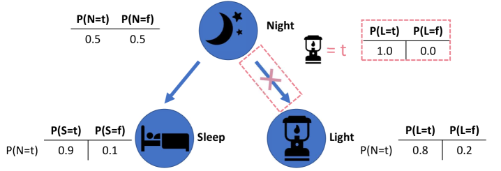
Figure 6: Performing differentiable causal reasoning and learning using NEMESYS. Given a causal Bayesian network, NEMESYS can easily perform the do operation (delete incoming edges) on arbitrary nodes and capture the causal effects on different nodes (for example, the probability of the node $\mathtt{Light}$ after intervening) without rerunning the entire system. Furthermore, NEMESYS is able to learn the unobserved $\mathtt{do}$ operation with its corresponding value using gradient descent based on the given causal graph and observed data. (Best viewed in color)
The $\mathtt{do}$ operator, denoted as $\mathtt{do(X)}$ , is used to represent an intervention on a particular variable $\mathtt{X}$ in a causal learning system, regardless of the actual value of the variable. For example, Fig. 6 shows a causal Bayesian network with three nodes and the probability distribution of the nodes before and after the $\mathtt{do}$ operation. To investigate how the node $\mathtt{Light}$ affects the rest of the system, we firstly cut the causal relationship between the node $\mathtt{Light}$ and all its parent nodes, then we assign a new value to the node and we investigate the probability of other nodes. To enable NEMESYS to perform a $\mathtt{do}$ operation on the node $\mathtt{Light}$ , we begin by representing the provided causal Bayesian network in Fig. 6 using:
| | $\displaystyle\mathtt{0.5}\texttt{:}\ \mathtt{Night}.\quad\mathtt{0.9}\texttt{: }\ \mathtt{Sleep}\texttt{:-}\mathtt{Night}.\quad\mathtt{0.8}\texttt{:}\ \mathtt{Light}\texttt{:-}\mathtt{Night}.$ | |
| --- | --- | --- |
where the number of an atom indicates the probability of the atom being true, and the number of a clause indicates the conditional probability of the head being true given the body being true.
We reuse the meta predicate $\mathtt{assert\_probs/1/[atom]}$ and introduce three new meta predicates: $\mathtt{prob/1/[atom]}$ , $\mathtt{probs/1/[atoms]}$ and $\mathtt{probs\_do/1/[atoms,atom]}$ . Since we cannot deal with the uncountable, infinite real numbers within our logic, we make use of the weight associated with ground meta atoms to represent the probability of the atom. For example, we use the weight of the meta atom $\mathtt{prob(Atom)}$ to represent the probability of the atom $\mathtt{Atom}$ . We use the weight of the meta atom $\mathtt{probs(Atoms)}$ to represent the joint probability of a list of atoms $\mathtt{Atoms}$ , and the weight of $\mathtt{probs\_do(AtomA,AtomB)}$ to represent the probability of the atom $\mathtt{AtomA}$ after performing the do operation $\mathtt{do(AtomB)}$ . We modify the meta interpreter as:
| | $\displaystyle\mathtt{prob(Head)}\texttt{:-}\mathtt{assert\_probs((Head\texttt{ :-}Body))},\mathtt{probs(Body).}$ | |
| --- | --- | --- |
where the first three rules calculate the probability of a node before the intervention, the joint probability is approximated using the first and second rule by iteratively multiplying each atom. The fourth rule assigns the probability of the atom $\mathtt{Atom}$ using the $\mathtt{do}$ operation. The fifth to the eighth calculate the probability after the $\mathtt{do}$ intervention by looping over each atom and multiplying them.
For example, after performing $\mathtt{do(Light)}$ and setting the probability of $\mathtt{Light}$ as $1.0$ . NEMESYS returns the weight of $\mathtt{probs\_do(Light,Light)}$ as the probability of the node $\mathtt{Light}$ (Fig. 6 red box) after the intervention $\mathtt{do(Light)}$ .
### 4.6 Gradient-based Learning in NEMESYS
NEMESYS alleviates the limitations of frameworks such as DeepProbLog [21] by having the ability of not only performing differentiable parameter learning but also supporting differentiable structure learning (in our experiment, NEMESYS learns the weights of the meta rules while adapting to solve different tasks). We now introduce the learning ability of NEMESYS.
#### 4.6.1 Parameter Learning
Consider a scenario in which a patient can only experience effective treatment when two types of medicine synergize, with the effectiveness contingent on the dosage of each drug. Suppose we have known the dosages of two medicines and the causal impact of the medicines on the patient, however, the observed effectiveness does not align with expectations. It is certain that some interventions have occurred in the medicine-patient causal structure (such as an incorrect dosage of one medicine, which will be treated as an intervention using the $\mathtt{do}$ operation). However, the specific node (patient or the medicines) on which the $\mathtt{do}$ operation is executed, and the values assigned to the $\mathtt{do}$ operator remain unknown. Conducting additional experiments on patients by altering medicine dosages to uncover the $\mathtt{do}$ operation is both unethical and dangerous.
With NEMESYS at hand, we can easily learn the unobserved $\mathtt{do}$ operation with its assigned value. We abstract the problem using a three-node causal Bayesian network:
$$
\mathtt{1.0:medicine\_a.}\quad\mathtt{1.0:medicine\_b.}\quad\mathtt{0.9:
patient}\texttt{:-}\mathtt{medicine\_a,medicine\_b.}
$$
where the number of the atoms indicates the dosage of each medicine, and the number of the clause indicates the conditional probability of the effectiveness of the patient given these two medicines. Suppose there is only one unobserved $\mathtt{do}$ operation.
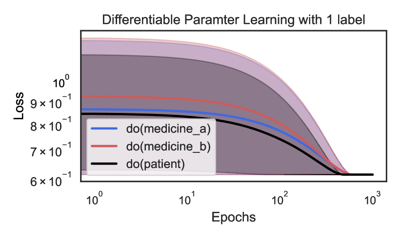
To learn the unknown $\mathtt{do}$ operation, we define the loss as the Binary Cross Entropy (BCE) loss between the observed probability $\mathbf{p}_{target}$ and the predicted probability of the target atom $\mathbf{p}_{predicted}$ . The predicted probability $\mathbf{p}_{predicted}$ is computed as: $\mathbf{p}_{predicted}=\mathbf{v}^{(T)}\left[I_{\mathcal{G}}(\operatorname{ target\_atom})\right]$ , where $I_{\mathcal{G}}(x)$ is a function that returns the index of target atom in $\mathcal{G}$ , $\mathbf{v}[i]$ is the $i$ -th element of $\mathbf{v}$ . $\mathbf{v}^{(T)}$ is the valuation tensor computed by $T$ -step forward reasoning based on the initial valuation tensor $\mathbf{v}^{(0)}$ , which is composed of the initial valuation of $\mathtt{do}$ and other meta ground atoms. Since the valuation of $\mathtt{do}$ atom is the only changing parameter, we set the gradient of other parameters as $0 0$ . We minimize the loss w.r.t. $\mathtt{do(X)}$ : $\underset{\mathtt{do(X)}}{\mathtt{minimize}}\quad\mathtt{L_{loss}}=\mathtt{BCE }(\mathbf{p}_{target},\mathbf{p}_{predicted}\mathtt{(do(X)))}.$ Fig. 7 summarizes the loss curve of the three $\mathtt{do}$ operators during learning using one target (Fig. 7 left) and three targets (Fig. 7 right). For the three targets experiment, $\mathbf{p}_{target}$ consists of three observed probabilities (the effectiveness of the patient and the dosages of two medicines), for the experiment with one target, $\mathbf{p}_{target}$ only consists of the observed the effectiveness of the patient.
We randomly initialize the probability of the three $\mathtt{do}$ operators and choose the one, which achieves the lowest loss as the right $\mathtt{do}$ operator. In the three targets experiment, the blue curve achieves the lowest loss, with its corresponding value converges to the ground truth value, while in the one target experiment, three $\mathtt{do}$ operators achieve equivalent performance. We provide the value curves of three $\mathtt{do}$ operators and the ground truth $\mathtt{do}$ operator with its value in Appendix C.
<details>
<summary>x6.png Details</summary>
### Visual Description
## Chart: Differentiable Parameter Learning with 1 label
### Overview
The image is a line chart showing the loss over epochs for three different conditions: "do(medicine_a)", "do(medicine_b)", and "do(patient)". The x-axis (Epochs) is on a logarithmic scale. Shaded regions around each line indicate uncertainty or variance.
### Components/Axes
* **Title:** Differentiable Parameter Learning with 1 label
* **X-axis:**
* Label: Epochs
* Scale: Logarithmic
* Markers: 10<sup>0</sup>, 10<sup>1</sup>, 10<sup>2</sup>, 10<sup>3</sup>
* **Y-axis:**
* Label: Loss
* Scale: Linear
* Markers: 6 x 10<sup>-1</sup>, 7 x 10<sup>-1</sup>, 8 x 10<sup>-1</sup>, 9 x 10<sup>-1</sup>, 10<sup>0</sup>
* **Legend:** Located in the center-left of the chart.
* Blue line: do(medicine\_a)
* Red line: do(medicine\_b)
* Black line: do(patient)
### Detailed Analysis
* **do(medicine\_a) (Blue):** The blue line starts at a loss of approximately 0.86 at epoch 1. It decreases slightly until around epoch 10, then decreases more rapidly until it plateaus at a loss of approximately 0.61 around epoch 100.
* **do(medicine\_b) (Red):** The red line starts at a loss of approximately 0.93 at epoch 1. It decreases gradually until around epoch 20, then decreases more rapidly until it plateaus at a loss of approximately 0.61 around epoch 100.
* **do(patient) (Black):** The black line starts at a loss of approximately 0.85 at epoch 1. It decreases more rapidly than the other two lines, reaching a loss of approximately 0.61 around epoch 50, and then remains relatively constant.
* **Shaded Regions:** Each line has a shaded region around it, indicating the variability or uncertainty in the loss. The shaded regions narrow as the number of epochs increases, suggesting that the model becomes more stable and consistent in its predictions.
### Key Observations
* All three conditions show a decrease in loss as the number of epochs increases, indicating that the model is learning.
* The "do(patient)" condition shows the fastest initial decrease in loss.
* All three conditions converge to a similar loss value (approximately 0.61) after a sufficient number of epochs.
* The uncertainty (shaded region) is highest at the beginning of training and decreases as training progresses.
### Interpretation
The chart demonstrates the learning curves for three different interventions or conditions. The "do(patient)" condition appears to be the most effective in reducing loss initially, suggesting that this intervention leads to faster learning. However, all three conditions eventually converge to a similar level of performance. The decreasing uncertainty over epochs indicates that the model becomes more reliable and consistent as it learns. The fact that all three converge to a similar loss value suggests that there may be a limit to how much the model can learn with the given data and architecture, or that the interventions have similar long-term effects.
</details>
<details>
<summary>x7.png Details</summary>
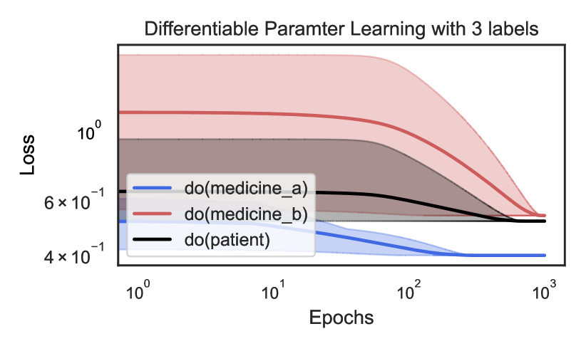
### Visual Description
## Chart: Differentiable Parameter Learning with 3 labels
### Overview
The image is a line chart showing the loss over epochs for three different conditions: "do(medicine_a)", "do(medicine_b)", and "do(patient)". Both axes are on a logarithmic scale. The chart displays how the loss changes as the number of epochs increases, with shaded regions around each line indicating variability or uncertainty.
### Components/Axes
* **Title:** Differentiable Parameter Learning with 3 labels
* **X-axis:** Epochs (logarithmic scale from 10^0 to 10^3)
* **Y-axis:** Loss (logarithmic scale from 4 x 10^-1 to 10^0)
* **Legend:** Located in the center-left of the chart.
* Blue line: do(medicine\_a)
* Red line: do(medicine\_b)
* Black line: do(patient)
### Detailed Analysis
* **do(medicine\_a) (Blue):** The blue line starts at approximately 0.5 (5 x 10^-1) at epoch 10^0 and decreases to approximately 0.4 (4 x 10^-1) by epoch 10^2, remaining relatively constant thereafter.
* **do(medicine\_b) (Red):** The red line starts at approximately 1.5 (1.5 x 10^0) at epoch 10^0 and decreases to approximately 0.5 (5 x 10^-1) by epoch 10^3.
* **do(patient) (Black):** The black line starts at approximately 0.7 (7 x 10^-1) at epoch 10^0, decreases slightly to approximately 0.6 (6 x 10^-1) around epoch 10^1, and then remains relatively constant at approximately 0.5 (5 x 10^-1) from epoch 10^2 to 10^3.
### Key Observations
* The loss for "do(medicine\_b)" starts highest but decreases the most over the epochs.
* The loss for "do(medicine\_a)" starts lowest and remains relatively low throughout.
* The loss for "do(patient)" starts in the middle and stabilizes at a similar level to "do(medicine\_a)" and "do(medicine\_b)" by the end of the observed epoch range.
* All three lines show a decrease in loss as the number of epochs increases, indicating learning or optimization.
### Interpretation
The chart illustrates the learning curves for three different conditions, likely in a machine learning or optimization context. The "loss" metric represents the error or cost associated with the model's predictions. The decrease in loss over epochs suggests that the model is improving its performance as it is trained. The different starting points and rates of decrease indicate that the conditions have different initial states or require different amounts of training to reach a stable performance level. The shaded regions likely represent the variance or uncertainty in the loss values, which could be due to factors such as data variability or model instability.
</details>
Figure 7: NEMESYS performs differentiable parameter learning using gradient descent. Based on the given data (one or three targets), NEMESYS is asked to learn the correct $\mathtt{do}$ operator and its corresponding value (which we didn’t show in the images). The loss curve is averaged on three runs. The shadow area indicates the min and max number of the three runs. (Best viewed in color)
<details>
<summary>x8.png Details</summary>
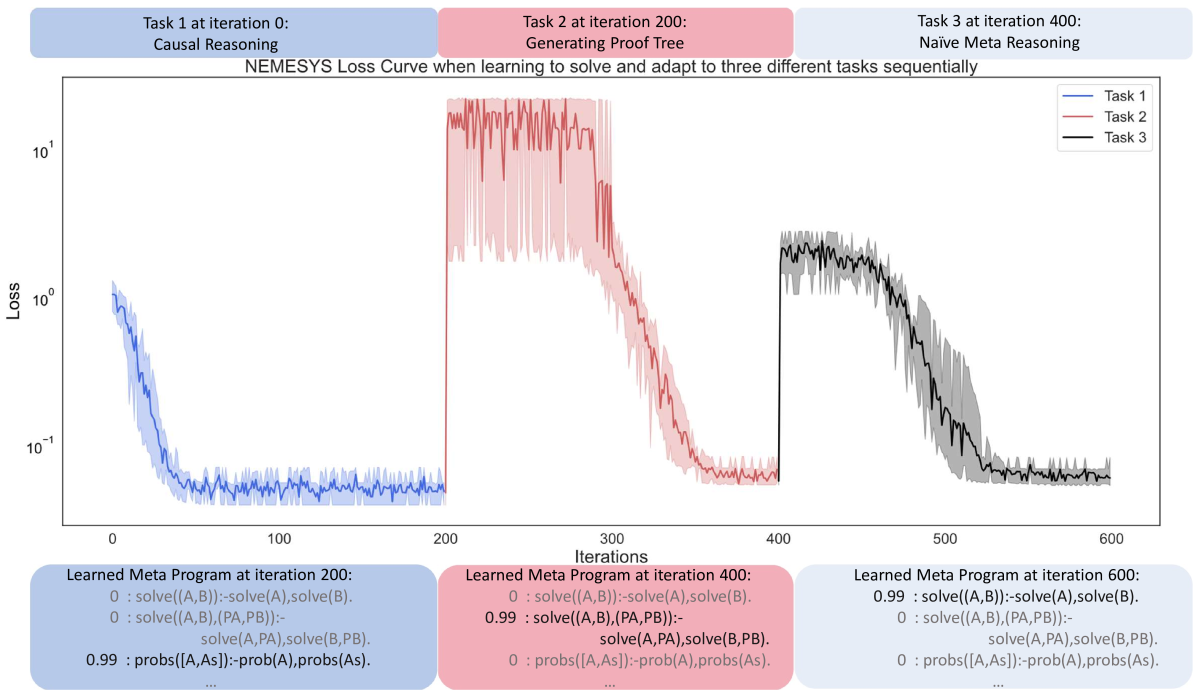
### Visual Description
## Loss Curve: NEMESYS Learning Across Tasks
### Overview
The image presents a loss curve illustrating the performance of the NEMESYS system as it learns to solve and adapt to three different tasks sequentially. The x-axis represents iterations, and the y-axis represents loss on a logarithmic scale. The plot shows three distinct phases, each corresponding to a different task: Causal Reasoning (Task 1), Generating Proof Tree (Task 2), and Naive Meta Reasoning (Task 3). The plot also includes learned meta programs at iterations 200, 400, and 600.
### Components/Axes
* **Title:** NEMESYS Loss Curve when learning to solve and adapt to three different tasks sequentially
* **X-axis:** Iterations, ranging from 0 to 600, with major ticks at 0, 100, 200, 300, 400, 500, and 600.
* **Y-axis:** Loss, on a logarithmic scale, ranging from 10<sup>-1</sup> to 10<sup>1</sup>, with major ticks at 10<sup>-1</sup>, 10<sup>0</sup>, and 10<sup>1</sup>.
* **Legend:** Located in the top-right corner.
* Task 1 (Blue)
* Task 2 (Red)
* Task 3 (Black)
* **Task Labels:**
* Task 1 at iteration 0: Causal Reasoning (Blue background)
* Task 2 at iteration 200: Generating Proof Tree (Red background)
* Task 3 at iteration 400: Naive Meta Reasoning (Pink background)
* **Learned Meta Programs:**
* Learned Meta Program at iteration 200 (Blue background)
* Learned Meta Program at iteration 400 (Red background)
* Learned Meta Program at iteration 600 (Blue background)
### Detailed Analysis
* **Task 1 (Blue):** Causal Reasoning. The loss decreases rapidly from approximately 10<sup>0</sup> at iteration 0 to approximately 10<sup>-1</sup> by iteration 100. The loss then stabilizes around 10<sup>-1</sup> for the remainder of the task's duration (until iteration 200).
* Learned Meta Program at iteration 200:
* `0 : solve((A,B)):-solve(A),solve(B).`
* `0 : solve((A,B),(PA,PB)):- solve(A,PA),solve(B,PB).`
* `0.99 : probs([A,As]):-prob(A),probs(As).`
* **Task 2 (Red):** Generating Proof Tree. The loss starts at approximately 10<sup>1</sup> at iteration 200 and decreases to approximately 10<sup>-1</sup> by iteration 400. The decrease is less rapid than in Task 1.
* Learned Meta Program at iteration 400:
* `0 : solve((A,B)):-solve(A),solve(B).`
* `0.99 : solve((A,B),(PA,PB)):- solve(A,PA),solve(B,PB).`
* `0 : probs([A,As]):-prob(A),probs(As).`
* **Task 3 (Black):** Naive Meta Reasoning. The loss starts at approximately 10<sup>0</sup> at iteration 400 and decreases to approximately 10<sup>-1</sup> by iteration 600. The decrease is relatively smooth.
* Learned Meta Program at iteration 600:
* `0.99 : solve((A,B)):-solve(A),solve(B).`
* `0 : solve((A,B),(PA,PB)):- solve(A,PA),solve(B,PB).`
* `0 : probs([A,As]):-prob(A),probs(As).`
### Key Observations
* Each task exhibits a decrease in loss over time, indicating learning.
* The initial loss for Task 2 is significantly higher than for Task 1, suggesting a more difficult initial state.
* The learned meta programs change over time, reflecting the adaptation to different tasks.
* The shaded regions around each line represent the variance or uncertainty in the loss values.
### Interpretation
The loss curve demonstrates the NEMESYS system's ability to learn and adapt to different tasks sequentially. The decreasing loss values indicate that the system is improving its performance on each task. The changes in the learned meta programs suggest that the system is modifying its internal representation to better suit the requirements of each task. The different initial loss values and learning rates for each task may reflect the varying complexity or difficulty of the tasks. The learned meta programs show the evolution of the system's reasoning rules as it progresses through the tasks. The system appears to be learning to solve problems more efficiently as it progresses through the tasks.
</details>
Figure 8: NEMESYS can learn to solve and adapt itself to different tasks during learning using gradient descent. In this experiment, we train NEMESYS to solve three different tasks: causal reasoning, generating proof trees and naive meta reasoning sequentially (each task is represented by a unique color encoding). The loss curve is averaged on five runs, with the shadow area indicating the minimum and maximum number of the five runs. For readability, the learned complete meta program is not shown in the image. (Best viewed in color)
#### 4.6.2 Structure Learning
Besides parameter learning, NEMESYS can also perform differentiable structure learning (we provide the candidate meta rules and learn the weights of these meta rules using gradient descent). In this experiment, different tasks are presented at distinct time steps throughout the learning process. NEMESYS is tasked with acquiring the ability to solve and adapt to these diverse tasks.
Following Sec. 3.2, we make use of the meta rule weight matrix $\mathbf{W}=[{\bf w}_{1},\ldots,{\bf w}_{M}]$ to select the rules. We take the softmax of each weight vector ${\bf w}_{j}\in\mathbf{W}$ to choose $M$ meta rules out of $C$ meta rules. To adapt to different tasks, the weight matrix $\mathbf{W}$ is learned based on the loss, which is defined as the BCE loss between the probability of the target $\mathbf{p}_{target}$ and the predicted probability $\mathbf{p}_{predicted}$ , where $\mathbf{p}_{predicted}$ is the probability of the target atoms calculated using the learned program. $\mathbf{p}_{predicted}$ is computed as: $\mathbf{p}_{predicted}=\mathbf{v}^{(T)}\left[I_{\mathcal{G}}(\operatorname{ target\_atoms})\right]$ , where $I_{\mathcal{G}}(x)$ is a function that returns the indexes of target atoms in $\mathcal{G}$ , $\mathbf{v}[i]$ is the $i$ -th element of $\mathbf{v}$ and $\mathbf{v}^{(T)}$ is the valuation tensor computed by $T$ -step forward reasoning. We minimize the loss w.r.t. the weight matrix $\mathbf{W}$ : $\underset{\mathbf{W}}{\mathtt{minimize}}\quad\mathtt{L_{loss}}=\mathtt{BCE}( \mathbf{p}_{target},\mathbf{p}_{predicted}(\mathbf{W})).$
We randomly initialize the weight matrix $\mathbf{W}$ , and update the weights using gradient descent. We set the target $\mathbf{p}_{target}$ using positive target atoms and negative target atoms. For example, suppose we have the naive meta reasoning and generating proof tree as two tasks. To learn a program to generate the proof tree, we use the proof tree meta rules to generate positive examples, and use the naive meta rules to generate the negative examples.
We ask NEMESYS to solve three different tasks sequentially, which is initially, calculating probabilities using the first three rules of causal reasoning, then executing naive meta-reasoning. Finally, generating a proof tree. We set the program size to three and randomly initialize the weight matrix. Fig. 8 shows the learning process of NEMESYS which can automatically adapt to solve these three different tasks. We provide the accuracy curve and the candidate rules with the learned weights in Appendix D. We also compare NEMESYS with the baseline method DeepProbLog [21] (cf. Table. 4). Due to the limitations of DeepProbLog in adapting (meta) rule weights during learning, we initialize DeepProbLog with three variants as our baseline comparisons. The first variant involves fixed task 1 meta rule weights ( $\mathtt{1.0}$ ), with task 2 and task 3 meta rule weights being randomly initialized. In the second variant, task 2 meta rule weights are fixed ( $\mathtt{1.0}$ ), while task 1 and task 3 meta rule weights are randomly initialized, and this pattern continues for the subsequent variant. We provide NEMESYS with the same candidate meta rules, however, with randomly initialize weights. We compute the accuracy at iteration $\mathtt{200}$ , $\mathtt{400}$ and $\mathtt{600}$ .
### 4.7 Discussion
While NEMESYS achieves impressive results, it is worth considering some of the limitations of this work. In our current experiments for structure learning, candidates of meta-rules are provided. It is promising to integrate rule-learning techniques, e.g., mode declarations, meta-interpretive learning, and a more sophisticated rule search, to learn from less prior. Another limitation lies in the calculation, since our system is not able to handle real number calculation, we make use of the weight associated with the atom to approximate the value and do the calculation.
| | Test Task1 | Test Task2 | Test Task3 |
| --- | --- | --- | --- |
| DeepProbLog (T1) | 100 $\bullet$ | 14.29 | 0 |
| DeepProbLog (T2) | 0 | 100 $\bullet$ | 11.43 |
| DeepProbLog (T3) | 68.57 | 5.71 | 100 $\bullet$ |
| NEMESYS (ours) | 100 $\bullet$ | 100 $\bullet$ | 100 $\bullet$ |
Table 4: Performance (Accuracy; the higher, the better) on test split of three tasks. We compare NEMESYS with baseline method DeepProbLog [21] (with three variants). The accuracy is averaged on five runs. The best-performing models are denoted using $\bullet$ .
## 5 Conclusions
We proposed the framework of neuro-metasymbolic reasoning and learning. We realized a differentiable meta interpreter using the differentiable implementation of first-order logic with meta predicates. This meta-interpreter, called NEMESYS, achieves various important functions on differentiable logic programming languages using meta-level programming. We illustrated this on different tasks of visual reasoning, reasoning with explanations, reasoning with infinite loops, planning on visual scenes, performing the $\mathtt{do}$ operation within a causal Bayesian network and showed NEMESYS’s gradient-based capability of parameter learning and structure learning.
NEMESYS provides several interesting avenues for future work. One major limitation of NEMESYS is its scalability for large-scale meta programs. So far, we have mainly focused on specifying the syntax and semantics of new (domain-specific) differentiable logic programming languages, helping to ensure that the languages have some desired properties. In the future, one should also explore providing properties about programs written in a particular differentiable logic programming language and injecting the properties into deep neural networks via algorithmic supervision [50], as well as program synthesis. Most importantly, since meta programs in NEMESYS are parameterized, and the reasoning mechanism is differentiable, one can realize differentiable meta-learning easily, i.e., the reasoning system that learns how to perform reasoning better from experiences.
Acknowledgements. This work was supported by the Hessian Ministry of Higher Education, Research, Science and the Arts (HMWK) cluster project “The Third Wave of AI”. The work has also benefited from the Hessian Ministry of Higher Education, Research, Science and the Arts (HMWK) cluster project “The Adaptive Mind” and the Federal Ministry for Economic Affairs and Climate Action (BMWK) AI lighthouse project “SPAICER” (01MK20015E), the EU ICT-48 Network of AI Research Excellence Center “TAILOR” (EU Horizon 2020, GA No 952215), and the Collaboration Lab “AI in Construction” (AICO) with Nexplore/HochTief.
## References
Ramesh et al. [2022] Ramesh, A., Dhariwal, P., Nichol, A., Chu, C., Chen, M.: Hierarchical text-conditional image generation with clip latents. arXiv Preprint:2204.0612 (2022)
Stiennon et al. [2020] Stiennon, N., Ouyang, L., Wu, J., Ziegler, D., Lowe, R., Voss, C., Radford, A., Amodei, D., Christiano, P.F.: Learning to summarize with human feedback. Advances in Neural Information Processing Systems (NeurIPS) (2020)
Floridi and Chiriatti [2020] Floridi, L., Chiriatti, M.: Gpt-3: Its nature, scope, limits, and consequences. Minds and Machines 30, 681–694 (2020)
Reed et al. [2022] Reed, S., Zolna, K., Parisotto, E., Colmenarejo, S.G., Novikov, A., Barth-maron, G., Giménez, M., Sulsky, Y., Kay, J., Springenberg, J.T., et al.: A generalist agent. Transactions on Machine Learning Research (TMLR) (2022)
Ackerman and Thompson [2017] Ackerman, R., Thompson, V.A.: Meta-reasoning: Monitoring and control of thinking and reasoning. Trends in cognitive sciences 21 (8), 607–617 (2017)
Costantini [2002] Costantini, S.: Meta-reasoning: A survey. In: Computational Logic: Logic Programming and Beyond (2002)
Griffiths et al. [2019] Griffiths, T.L., Callaway, F., Chang, M.B., Grant, E., Krueger, P.M., Lieder, F.: Doing more with less: Meta-reasoning and meta-learning in humans and machines. Current Opinion in Behavioral Sciences 29, 24–30 (2019)
Russell and Wefald [1991] Russell, S., Wefald, E.: Principles of metareasoning. Artificial intelligence 49 (1-3), 361–395 (1991)
Schmidhuber [1987] Schmidhuber, J.: Evolutionary principles in self-referential learning, or on learning how to learn: the meta-meta-… hook. PhD thesis, Technische Universität München (1987)
Thrun and Pratt [1998] Thrun, S., Pratt, L.: Learning to Learn: Introduction and Overview, pp. 3–17. Springer, Boston, MA (1998)
Finn et al. [2017] Finn, C., Abbeel, P., Levine, S.: Model-agnostic meta-learning for fast adaptation of deep networks. In: Proceedings of the 34th International Conference on Machine Learning (ICML) (2017)
Hospedales et al. [2022] Hospedales, T.M., Antoniou, A., Micaelli, P., Storkey, A.J.: Meta-learning in neural networks: A survey. IEEE Trans. Pattern Anal. Mach. Intell. 44 (9), 5149–5169 (2022)
Kim et al. [2018] K im, J., Ricci, M., Serre, T.: Not-so-clevr: learning same–different relations strains feedforward neural networks. Interface focus (2018)
Stammer et al. [2021] Stammer, W., Schramowski, P., Kersting, K.: Right for the right concept: Revising neuro-symbolic concepts by interacting with their explanations. In: Proceedings of the IEEE Conference on Computer Vision and Pattern Recognition (CVPR) (2021)
Shindo et al. [2021] Shindo, H., Dhami, D.S., Kersting, K.: Neuro-symbolic forward reasoning. arXiv Preprint:2110.09383 (2021)
Evans and Grefenstette [2018] Evans, R., Grefenstette, E.: Learning explanatory rules from noisy data. J. Artif. Intell. Res. 61, 1–64 (2018)
Shindo et al. [2021] Shindo, H., Nishino, M., Yamamoto, A.: Differentiable inductive logic programming for structured examples. In: Proceedings of the 35th AAAI Conference on Artificial Intelligence (AAAI) (2021)
Johnson et al. [2017] Johnson, J., Hariharan, B., Maaten, L., Fei-Fei, L., Zitnick, C.L., Girshick, R.B.: Clevr: A diagnostic dataset for compositional language and elementary visual reasoning. Proceedings of the IEEE Conference on Computer Vision and Pattern Recognition (CVPR) (2017)
Holzinger et al. [2019] Holzinger, A., Kickmeier-Rust, M., Müller, H.: Kandinsky patterns as iq-test for machine learning. In: Proceedings of the 3rd International Cross-Domain Conference for Machine Learning and Knowledge Extraction (CD-MAKE) (2019)
Müller and Holzinger [2021] Müller, H., Holzinger, A.: Kandinsky patterns. Artificial Intelligence 300, 103546 (2021)
Manhaeve et al. [2018] Manhaeve, R., Dumancic, S., Kimmig, A., Demeester, T., De Raedt, L.: Deepproblog: Neural probabilistic logic programming. Advances in Neural Information Processing Systems (NeurIPS) (2018)
Rocktäschel and Riedel [2017] Rocktäschel, T., Riedel, S.: End-to-end differentiable proving. Advances in neural information processing systems 30 (2017)
Cunnington et al. [2023] Cunnington, D., Law, M., Lobo, J., Russo, A.: Ffnsl: feed-forward neural-symbolic learner. Machine Learning 112 (2), 515–569 (2023)
Shindo et al. [2023] Shindo, H., Pfanschilling, V., Dhami, D.S., Kersting, K.: $\alpha$ ilp: thinking visual scenes as differentiable logic programs. Machine Learning 112, 1465–1497 (2023)
Huang et al. [2021] Huang, J., Li, Z., Chen, B., Samel, K., Naik, M., Song, L., Si, X.: Scallop: From probabilistic deductive databases to scalable differentiable reasoning. Advances in Neural Information Processing Systems (NeurIPS) (2021)
Yang et al. [2020] Yang, Z., Ishay, A., Lee, J.: Neurasp: Embracing neural networks into answer set programming. In: Proceedings of the 29th International Joint Conference on Artificial Intelligence, (IJCAI) (2020)
Pearl [2009] Pearl, J.: Causality. Cambridge university press, Cambridge (2009)
Pearl [2012] Pearl, J.: The do-calculus revisited. In: Proceedings of the 28th Conference on Uncertainty in Artificial Intelligence (UAI) (2012)
Russell and Norvig [2009] Russell, S., Norvig, P.: Artificial Intelligence: A Modern Approach, 3rd edn. Prentice Hall Press, Hoboken, New Jersey (2009)
Jiang and Luo [2019] Jiang, Z., Luo, S.: Neural logic reinforcement learning. In: Proceedings of the 36th International Conference on Machine Learning (ICML) (2019)
Delfosse et al. [2023] Delfosse, Q., Shindo, H., Dhami, D., Kersting, K.: Interpretable and explainable logical policies via neurally guided symbolic abstraction. arXiv preprint arXiv:2306.01439 (2023)
Maes and Nardi [1988] Maes, P., Nardi, D.: Meta-Level Architectures and Reflection. Elsevier Science Inc., USA (1988)
Lloyd [1984] Lloyd, J.W.: Foundations of Logic Programming, 1st Edition. Springer, Heidelberg (1984)
Hill and Gallagher [1998] Hill, P.M., Gallagher, J.: Meta-Programming in Logic Programming. Oxford University Press, Oxford (1998)
Pettorossi [1992] Pettorossi, A. (ed.): Proceedings of the 3rd International Workshop of Meta-Programming in Logic, (META). Lecture Notes in Computer Science, vol. 649 (1992)
Apt and Turini [1995] Apt, K.R., Turini, F.: Meta-Logics and Logic Programming. MIT Press (MA), Massachusett (1995)
Sterling and Shapiro [1994] Sterling, L., Shapiro, E.Y.: The Art of Prolog: Advanced Programming Techniques. MIT press, Massachusett (1994)
Muggleton et al. [2014a] Muggleton, S.H., Lin, D., Pahlavi, N., Tamaddoni-Nezhad, A.: Meta-interpretive learning: application to grammatical inference. Machine learning 94, 25–49 (2014)
Muggleton et al. [2014b] Muggleton, S.H., Lin, D., Chen, J., Tamaddoni-Nezhad, A.: Metabayes: Bayesian meta-interpretative learning using higher-order stochastic refinement. Proceedings of the 24th International Conference on Inductive Logic Programming (ILP) (2014)
Muggleton et al. [2015] Muggleton, S.H., Lin, D., Tamaddoni-Nezhad, A.: Meta-interpretive learning of higher-order dyadic datalog: Predicate invention revisited. Machine Learning 100, 49–73 (2015)
Cuturi and Blondel [2017] Cuturi, M., Blondel, M.: Soft-dtw: a differentiable loss function for time-series. In: Proceedings of the 34th International Conference on Machine Learning (ICML) (2017)
Redmon et al. [2016] Redmon, J., Divvala, S., Girshick, R., Farhadi, A.: You only look once: Unified, real-time object detection. In: Proceedings of the IEEE Conference on Computer Vision and Pattern Recognition (CVPR) (2016)
Holzinger et al. [2021] Holzinger, A., Saranti, A., Müller, H.: Kandinsky patterns - an experimental exploration environment for pattern analysis and machine intelligence. arXiv Preprint:2103.00519 (2021)
He et al. [2016] He, K., Zhang, X., Ren, S., Sun, J.: Deep residual learning for image recognition. In: Proceedings of the IEEE Conference on Computer Vision and Pattern Recognition (CVPR) (2016)
Locatello et al. [2020] Locatello, F., Weissenborn, D., Unterthiner, T., Mahendran, A., Heigold, G., Uszkoreit, J., Dosovitskiy, A., Kipf, T.: Object-centric learning with slot attention. Advances in Neural Information Processing Systems (NeurIPS) (2020)
Lee et al. [2019] Lee, J., Lee, Y., Kim, J., Kosiorek, A., Choi, S., Teh, Y.W.: Set transformer: A framework for attention-based permutation-invariant neural networks. In: Proceedings of the 36th International Conference on Machine Learning (ICML) (2019)
De Raedt et al. [2007] De Raedt, L., Kimmig, A., Toivonen, H.: Problog: A probabilistic prolog and its application in link discovery. In: IJCAI, vol. 7, pp. 2462–2467 (2007). Hyderabad
Lapuschkin et al. [2019] Lapuschkin, S., Wäldchen, S., Binder, A., Montavon, G., Samek, W., Müller, K.-R.: Unmasking clever hans predictors and assessing what machines really learn. Nature communications 10 (2019)
Kwisthout [2011] Kwisthout, J.: Most probable explanations in bayesian networks: Complexity and tractability. International Journal of Approximate Reasoning 52 (9), 1452–1469 (2011)
Petersen et al. [2021] Petersen, F., Borgelt, C., Kuehne, H., Deussen, O.: Learning with algorithmic supervision via continuous relaxations. In: Advances in Neural Information Processing Systems (NeurIPS) (2021)
## Appendix A Queries for Avoiding Infinite Loop
We use four queries to test the performance of NEMESYS and ProbLog [47].The four queries include one query which calls the recursive rule. The queries are:
| | $\displaystyle\mathtt{query(path(a,a,[]))}.\quad\mathtt{query(path(b,b,[]))}.$ | |
| --- | --- | --- |
## Appendix B Differentiable Planning
We provide more planning tasks in Figure. 9 with varying numbers of objects and attributes. Given the initial states and goal states, NEMESYS is asked to provide the intermediate steps to move different objects from start states to the end states.
<details>
<summary>extracted/5298395/images/clever-beforemove1.png Details</summary>
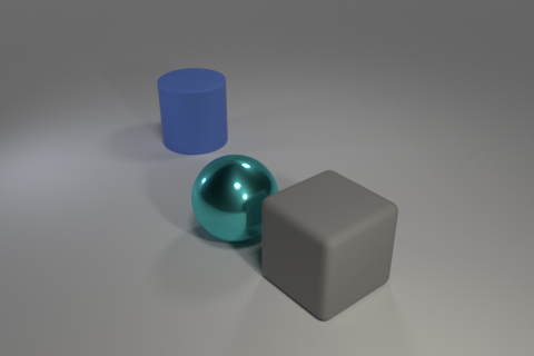
### Visual Description
## 3D Render: Geometric Shapes
### Overview
The image is a 3D render featuring three geometric shapes: a blue cylinder, a teal sphere, and a gray cube. They are arranged on a light gray surface with soft lighting and shadows.
### Components/Axes
* **Shapes:** Cylinder, Sphere, Cube
* **Colors:** Blue, Teal, Gray
* **Surface:** Light Gray
### Detailed Analysis or ### Content Details
* **Cylinder:** Located in the top-left quadrant of the image. It is a solid blue color.
* **Sphere:** Positioned between the cylinder and the cube, slightly overlapping both. It has a reflective teal surface.
* **Cube:** Situated in the bottom-right quadrant. It is a solid gray color with rounded edges.
* **Surface:** The shapes are resting on a light gray surface. Shadows are cast behind each shape, indicating a light source from the top-left.
### Key Observations
* The shapes are arranged in a non-uniform manner, suggesting a deliberate composition rather than a random placement.
* The reflective surface of the sphere adds visual interest and contrasts with the matte surfaces of the cylinder and cube.
* The lighting and shadows contribute to the depth and realism of the render.
### Interpretation
The image appears to be a simple 3D composition showcasing basic geometric shapes. The choice of colors and the reflective surface of the sphere suggest an aesthetic intent. The image could be used for educational purposes, demonstrating basic 3D rendering techniques, or as a visual element in a design project. The arrangement of the shapes and the lighting create a visually balanced and appealing composition.
</details>
<details>
<summary>extracted/5298395/images/clever-beforemove2.png Details</summary>
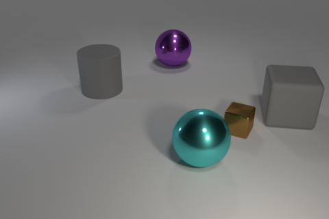
### Visual Description
## Still Life: Geometric Shapes
### Overview
The image is a still life featuring several geometric shapes arranged on a light gray surface. The shapes include a cylinder, two spheres (one purple and one teal), and two cubes (one gray and one gold). The lighting is soft, creating subtle shadows that define the forms.
### Components/Axes
* **Shapes:** Cylinder, Purple Sphere, Teal Sphere, Gold Cube, Gray Cube
* **Colors:** Light Gray, Purple, Teal, Gold
* **Arrangement:** The shapes are scattered across the surface, with the cylinder on the left, the purple sphere near the top, the teal sphere and gold cube in the center, and the gray cube on the right.
### Detailed Analysis
* **Cylinder:** Located on the left side of the image. It is gray and appears to be a solid, opaque object.
* **Purple Sphere:** Positioned near the top-center of the image. It has a metallic sheen, reflecting light.
* **Teal Sphere:** Situated in the lower-center of the image. It also has a metallic, reflective surface.
* **Gold Cube:** Placed between the teal sphere and the gray cube. It is smaller than the gray cube and has a highly reflective, metallic surface.
* **Gray Cube:** Located on the right side of the image. It is a solid, opaque object, similar in color to the cylinder.
* **Surface:** The shapes rest on a light gray surface that appears to be smooth and reflective.
### Key Observations
* The image showcases a variety of geometric shapes with different colors and surface properties (opaque vs. reflective).
* The arrangement of the shapes is somewhat random, creating a visually balanced composition.
* The lighting is soft and even, highlighting the forms and textures of the objects.
### Interpretation
The image is a study in form, color, and light. The arrangement of the geometric shapes creates a sense of visual harmony, while the different colors and surface properties add interest and complexity. The image could be interpreted as an exploration of basic geometric forms or as a purely aesthetic composition. The metallic spheres contrast with the matte cubes and cylinder, adding visual interest. The gold cube acts as a focal point due to its small size and reflective surface.
</details>
<details>
<summary>extracted/5298395/images/clever-aftermove1.png Details</summary>
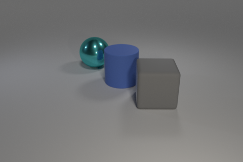
### Visual Description
## Geometric Shapes: 3D Rendering
### Overview
The image is a 3D rendering featuring three geometric shapes: a sphere, a cylinder, and a cube. They are positioned on a flat, light-colored surface with a gradient background.
### Components/Axes
* **Sphere:** Located on the left side of the image, it has a teal, metallic appearance.
* **Cylinder:** Positioned to the right of the sphere, it is a solid blue color.
* **Cube:** Situated to the right of the cylinder, it is a solid gray color.
* **Surface:** The shapes rest on a light gray surface.
* **Background:** The background is a gradient, transitioning from a lighter shade at the bottom to a darker shade at the top.
### Detailed Analysis
* **Sphere:** The sphere is reflective, showing highlights and shadows that suggest a light source from the upper left.
* **Cylinder:** The cylinder is a uniform blue color with no visible texture or reflections.
* **Cube:** The cube is a uniform gray color with no visible texture or reflections.
* **Arrangement:** The shapes are arranged in a row, with the sphere slightly behind the cylinder, and the cylinder slightly behind the cube.
* **Shadows:** Each shape casts a shadow on the surface, indicating a light source from the upper left.
### Key Observations
* The rendering appears to be a simple demonstration of 3D shapes and lighting.
* The use of different colors and materials (metallic vs. solid) adds visual interest.
* The shadows provide depth and grounding to the scene.
### Interpretation
The image likely serves as a basic example of 3D rendering capabilities. The arrangement of the shapes and the lighting suggest a focus on showcasing the different forms and their interaction with light and shadow. The simplicity of the scene makes it suitable for educational or demonstrative purposes.
</details>
<details>
<summary>extracted/5298395/images/clever-aftermove2.png Details</summary>
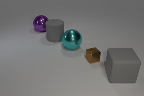
### Visual Description
## Still Life: Geometric Shapes
### Overview
The image is a still life featuring five geometric shapes arranged on a light gray surface. The shapes, from left to right, are a purple sphere, a gray cylinder, a teal sphere, a gold cube, and a gray cube. The lighting is soft, creating reflections on the spheres and cube.
### Components/Axes
* **Shapes:** Sphere, Cylinder, Cube
* **Colors:** Purple, Gray, Teal, Gold
* **Arrangement:** Linear, from left to right
### Detailed Analysis or ### Content Details
* **Purple Sphere:** Located on the left side of the image. It is highly reflective.
* **Gray Cylinder:** Positioned to the right of the purple sphere. It has a matte finish.
* **Teal Sphere:** Situated to the right of the gray cylinder. It is highly reflective.
* **Gold Cube:** Placed to the right of the teal sphere. It is reflective.
* **Gray Cube:** Located on the right side of the image. It has a matte finish and is larger than the gold cube.
### Key Observations
* The shapes are arranged in a linear fashion, with the spheres on the left and the cubes on the right.
* The colors alternate between vibrant (purple, teal, gold) and neutral (gray).
* The reflective surfaces of the spheres and gold cube contrast with the matte surfaces of the gray cylinder and cube.
* The size of the shapes generally increases from left to right.
### Interpretation
The image appears to be a study in geometric forms and material properties. The arrangement of the shapes, the contrast in colors and textures, and the soft lighting create a visually appealing composition. The image could be used to illustrate basic geometric shapes, color theory, or the effects of light on different materials. The arrangement of the shapes could also be interpreted as a progression or sequence, with the spheres representing a starting point and the cubes representing an end point.
</details>
Figure 9: Visual Concept Repairing: NEMESYS achieves planning by performing differentiable meta-level reasoning. The left two images show the start state, and the right two images show the goal state. Taking these states as inputs, NEMESYS performs differentiable forward reasoning using meta-level clauses that simulate the planning steps and generate actions from start state to reach the goal state. (Best viewed in color)
## Appendix C Differentiable Parameter Learning Value Curve
We also provide the corresponding value curve of these different $\mathtt{do}$ operators during learning in Fig. 10. In the experiment, we choose the $\mathtt{do}$ operator which achieves the lowest value as the correct value, thus in the experiment with three targets, we choose $\mathtt{do(medicine\_a)}$ with value $0.8$ , which is exactly the ground-truth $\mathtt{do}$ operator with the correct number.
<details>
<summary>x9.png Details</summary>
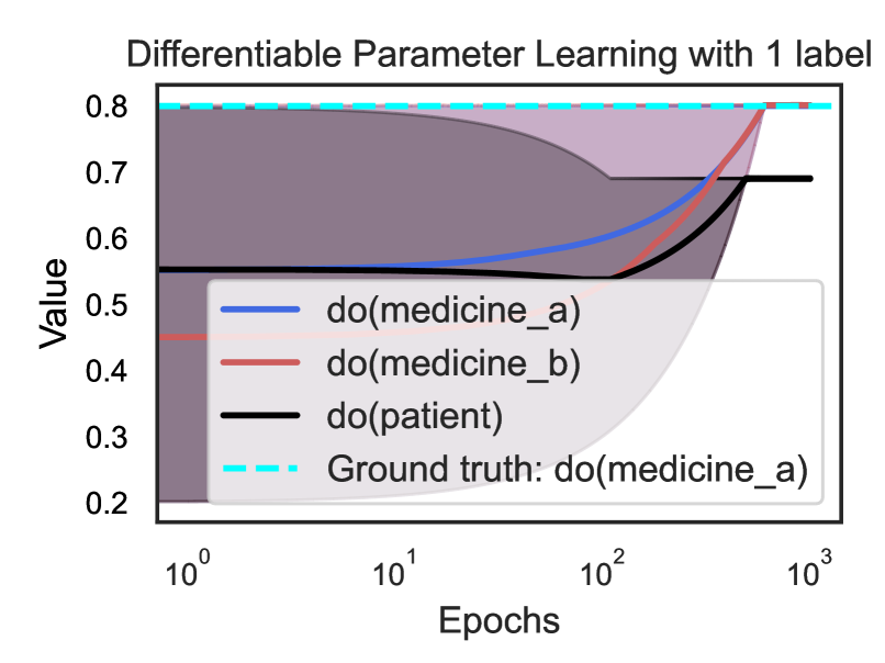
### Visual Description
## Line Chart: Differentiable Parameter Learning with 1 label
### Overview
The image is a line chart titled "Differentiable Parameter Learning with 1 label". It displays the change in "Value" over "Epochs" for three different interventions: "do(medicine_a)", "do(medicine_b)", and "do(patient)", along with a "Ground truth: do(medicine_a)". The x-axis (Epochs) is on a logarithmic scale. Shaded regions around the lines indicate uncertainty.
### Components/Axes
* **Title:** Differentiable Parameter Learning with 1 label
* **X-axis:**
* Label: Epochs
* Scale: Logarithmic (base 10)
* Markers: 10<sup>0</sup>, 10<sup>1</sup>, 10<sup>2</sup>, 10<sup>3</sup>
* **Y-axis:**
* Label: Value
* Scale: Linear
* Markers: 0.2, 0.3, 0.4, 0.5, 0.6, 0.7, 0.8
* **Legend:** Located in the center of the chart.
* Blue line: do(medicine\_a)
* Red line: do(medicine\_b)
* Black line: do(patient)
* Cyan dashed line: Ground truth: do(medicine\_a)
### Detailed Analysis
* **do(medicine\_a) (Blue):** The blue line starts at a value of approximately 0.52 at 10<sup>0</sup> epochs. It increases gradually until approximately 10<sup>2</sup> epochs, then increases more rapidly, reaching a value of approximately 0.7 at 10<sup>3</sup> epochs.
* **do(medicine\_b) (Red):** The red line starts at a value of approximately 0.45 at 10<sup>0</sup> epochs. It remains relatively flat until approximately 10<sup>2</sup> epochs, then increases rapidly, reaching a value of approximately 0.78 at 10<sup>3</sup> epochs.
* **do(patient) (Black):** The black line starts at a value of approximately 0.55 at 10<sup>0</sup> epochs. It remains relatively flat until approximately 10<sup>2</sup> epochs, then increases slightly, reaching a value of approximately 0.69 at 10<sup>3</sup> epochs.
* **Ground truth: do(medicine\_a) (Cyan Dashed):** The cyan dashed line remains constant at a value of approximately 0.8 across all epochs.
### Key Observations
* The "Ground truth: do(medicine\_a)" serves as a benchmark, remaining constant throughout the epochs.
* "do(medicine\_a)" and "do(medicine\_b)" show significant increases in "Value" after 10<sup>2</sup> epochs.
* "do(patient)" shows a much smaller increase in "Value" compared to the medicine interventions.
* The shaded regions around the lines indicate the uncertainty in the estimated "Value" for each intervention. The uncertainty appears to decrease as the number of epochs increases, particularly for "do(medicine\_a)" and "do(medicine\_b)".
### Interpretation
The chart illustrates the learning process of a model attempting to predict the outcome of different interventions ("do(medicine\_a)", "do(medicine\_b)", "do(patient)") compared to a known "Ground truth" for "do(medicine\_a)". The x-axis represents the training progress (epochs), and the y-axis represents the model's performance ("Value").
The data suggests that the model learns to predict the effect of "do(medicine\_a)" and "do(medicine\_b)" more effectively as the number of epochs increases, as indicated by the increasing "Value" and decreasing uncertainty. The "do(patient)" intervention shows a less pronounced learning curve, suggesting that the model struggles to accurately predict its effect.
The convergence of "do(medicine\_a)" and "do(medicine\_b)" towards the "Ground truth" indicates that the model is successfully learning the underlying causal relationships. The slower convergence of "do(patient)" might indicate a more complex or less predictable relationship.
</details>
<details>
<summary>x10.png Details</summary>
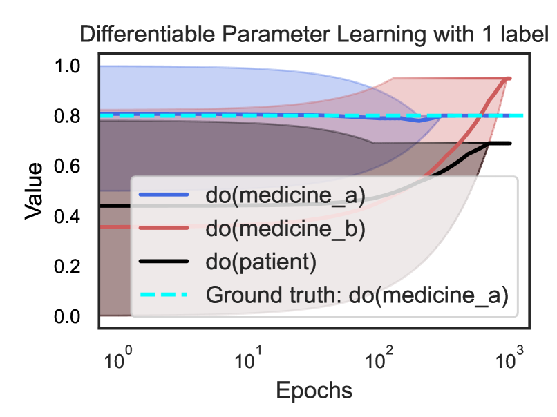
### Visual Description
## Line Chart: Differentiable Parameter Learning with 1 label
### Overview
The image is a line chart titled "Differentiable Parameter Learning with 1 label". It displays the change in "Value" over "Epochs" for three different interventions: "do(medicine_a)", "do(medicine_b)", and "do(patient)", along with a "Ground truth" line for "do(medicine_a)". The x-axis (Epochs) is on a logarithmic scale.
### Components/Axes
* **Title:** Differentiable Parameter Learning with 1 label
* **X-axis:**
* Label: Epochs
* Scale: Logarithmic (base 10)
* Markers: 10⁰, 10¹, 10², 10³
* **Y-axis:**
* Label: Value
* Scale: Linear
* Markers: 0.0, 0.2, 0.4, 0.6, 0.8, 1.0
* **Legend:** Located in the center of the chart.
* Blue line: do(medicine\_a)
* Red line: do(medicine\_b)
* Black line: do(patient)
* Cyan dashed line: Ground truth: do(medicine\_a)
### Detailed Analysis
* **do(medicine\_a) (Blue):** The blue line starts at a value of approximately 1.0 and decreases slightly to around 0.8 between 10¹ and 10².
* At Epoch 10⁰: Value ≈ 1.0
* At Epoch 10¹: Value ≈ 0.95
* At Epoch 10²: Value ≈ 0.8
* At Epoch 10³: Value ≈ 0.8
* **do(medicine\_b) (Red):** The red line starts at a value of approximately 0.35, remains relatively constant until around 10², and then increases sharply to approximately 0.95 at 10³.
* At Epoch 10⁰: Value ≈ 0.35
* At Epoch 10¹: Value ≈ 0.35
* At Epoch 10²: Value ≈ 0.35
* At Epoch 10³: Value ≈ 0.95
* **do(patient) (Black):** The black line starts at a value of approximately 0.45 and increases gradually to approximately 0.7 at 10³.
* At Epoch 10⁰: Value ≈ 0.45
* At Epoch 10¹: Value ≈ 0.45
* At Epoch 10²: Value ≈ 0.6
* At Epoch 10³: Value ≈ 0.7
* **Ground truth: do(medicine\_a) (Cyan Dashed):** The cyan dashed line remains constant at a value of approximately 0.8 across all epochs.
* At Epoch 10⁰: Value ≈ 0.8
* At Epoch 10¹: Value ≈ 0.8
* At Epoch 10²: Value ≈ 0.8
* At Epoch 10³: Value ≈ 0.8
### Key Observations
* "do(medicine\_a)" starts with a high value and decreases slightly.
* "do(medicine\_b)" shows a significant increase in value after 10² epochs.
* "do(patient)" shows a gradual increase in value over the epochs.
* "Ground truth: do(medicine\_a)" remains constant throughout the epochs.
### Interpretation
The chart illustrates the learning process of different interventions over epochs. "do(medicine\_b)" shows a delayed but significant improvement, suggesting it might require more epochs to reach its potential. "do(patient)" shows a steady but less dramatic improvement. "do(medicine\_a)" starts with a high value, possibly indicating a good initial state, but its value decreases slightly over time. The "Ground truth" line serves as a benchmark for the "do(medicine\_a)" intervention, indicating that the learned parameter for "do(medicine\_a)" converges towards the ground truth value after a certain number of epochs. The shaded regions around each line likely represent the uncertainty or variance in the learning process.
</details>
Figure 10: Value curve of three $\mathtt{do}$ operators during learning. With three targets (right) and with one target (left). The curves are averaged on 5 runs, with shaded area indicating the maximum and minimum value. (Best viewed in color)
## Appendix D Multi-Task Adaptation
<details>
<summary>x11.png Details</summary>
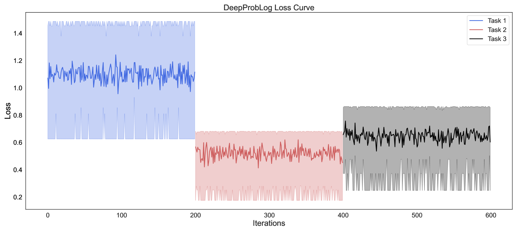
### Visual Description
## Line Chart: DeepProbLog Loss Curve
### Overview
The image is a line chart titled "DeepProbLog Loss Curve". It displays the loss values for three tasks (Task 1, Task 2, and Task 3) over a range of iterations. Each task's loss is represented by a different colored line: blue for Task 1, red for Task 2, and black for Task 3. The chart shows how the loss changes over iterations for each task.
### Components/Axes
* **Title:** DeepProbLog Loss Curve
* **X-axis:** Iterations, with tick marks at 0, 100, 200, 300, 400, 500, and 600.
* **Y-axis:** Loss, with tick marks at 0.2, 0.4, 0.6, 0.8, 1.0, 1.2, and 1.4.
* **Legend:** Located in the top-right corner, it identifies the lines as:
* Task 1 (blue)
* Task 2 (red)
* Task 3 (black)
### Detailed Analysis
* **Task 1 (Blue):** The blue line representing Task 1 starts at iteration 0 and extends to approximately iteration 200. The loss fluctuates around an average value of approximately 1.1, with variations between approximately 0.6 and 1.5.
* **Task 2 (Red):** The red line representing Task 2 starts at approximately iteration 200 and extends to approximately iteration 400. The loss fluctuates around an average value of approximately 0.5, with variations between approximately 0.2 and 0.7.
* **Task 3 (Black):** The black line representing Task 3 starts at approximately iteration 400 and extends to approximately iteration 600. The loss fluctuates around an average value of approximately 0.7, with variations between approximately 0.4 and 0.9.
### Key Observations
* Each task is active for a specific range of iterations.
* Task 1 has the highest loss values, followed by Task 3, and then Task 2.
* The loss values for each task fluctuate, indicating variations in performance during training.
### Interpretation
The chart illustrates the training progress of three different tasks within the DeepProbLog framework. The loss curve for each task shows how well the model is learning over iterations. The fact that each task is active for a specific range of iterations suggests a sequential or staged training process. The different loss values indicate varying levels of difficulty or complexity for each task. The fluctuations in loss suggest that the model is still learning and adapting during the active iterations for each task.
</details>
Figure 11: DeepProbLog [21] is initialized using the same candidate meta rules (also with randomized meta rule weights as NEMESYS). The loss curve is averaged on five runs, with the shadow area indicating the minimum and maximum number of the five runs. (Best viewed in color)
<details>
<summary>x12.png Details</summary>
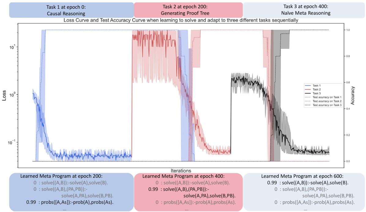
### Visual Description
## Loss and Accuracy Curve: Learning to Solve and Adapt
### Overview
The image presents a line chart illustrating the loss and test accuracy curves of a model learning to solve and adapt to three different tasks sequentially. The chart displays the loss on a logarithmic scale on the left y-axis and accuracy on a linear scale on the right y-axis, plotted against iterations on the x-axis. The chart is segmented into three distinct phases, each corresponding to a different task. The tasks are: Task 1 (Causal Reasoning), Task 2 (Generating Proof Tree), and Task 3 (Naive Meta Reasoning). The chart also includes learned meta programs at epochs 200, 400, and 600.
### Components/Axes
* **Title:** Loss Curve and Test Accuracy Curve when learning to solve and adapt to three different tasks sequentially
* **X-axis:** Iterations
* **Left Y-axis:** Loss (logarithmic scale)
* Axis markers: 10^-1, 10^0, 10^1
* **Right Y-axis:** Accuracy (linear scale)
* Axis markers: 0.0, 0.2, 0.4, 0.6, 0.8, 1.0
* **Legend:** Located on the right side of the chart.
* Task 1 (Blue solid line)
* Task 2 (Red solid line)
* Task 3 (Black solid line)
* Test accuracy on Task 1 (Blue dotted line)
* Test accuracy on Task 2 (Red dotted line)
* Test accuracy on Task 3 (Black dotted line)
* **Task Labels:**
* Task 1 at epoch 0: Causal Reasoning (Top-left, light blue background)
* Task 2 at epoch 200: Generating Proof Tree (Top-center, light red background)
* Task 3 at epoch 400: Naive Meta Reasoning (Top-right, light grey background)
* **Learned Meta Program Blocks:**
* Learned Meta Program at epoch 200 (Bottom-left, light blue background)
* Learned Meta Program at epoch 400 (Bottom-center, light red background)
* Learned Meta Program at epoch 600 (Bottom-right, light grey background)
### Detailed Analysis
* **Task 1 (Blue):**
* **Loss (Blue solid line):** Starts at approximately 10^1, decreases rapidly to around 10^-1 within the first ~50 iterations, and then stabilizes around 10^-1.
* **Test Accuracy (Blue dotted line):** Starts near 0.0, increases rapidly to approximately 1.0 within the first ~50 iterations, and then remains stable at 1.0.
* **Task 2 (Red):**
* **Loss (Red solid line):** Starts at approximately 10^1, decreases to around 10^-1 between iterations ~200 and ~300.
* **Test Accuracy (Red dotted line):** Starts near 0.0, increases to approximately 1.0 between iterations ~200 and ~300, and then remains stable at 1.0.
* **Task 3 (Black):**
* **Loss (Black solid line):** Starts at approximately 0.6 (estimated log scale value), decreases to around 0.1 between iterations ~400 and ~500.
* **Test Accuracy (Black dotted line):** Starts near 0.0, increases to approximately 1.0 between iterations ~400 and ~500, and then remains stable at 1.0.
* **Learned Meta Programs:**
* **Epoch 200 (Blue):**
* `0 : solve((A,B)):-solve(A),solve(B).`
* `0 : solve((A,B),(PA,PB)):- solve(A,PA),solve(B,PB).`
* `0.99 : probs([A,As]):-prob(A),probs(As).`
* **Epoch 400 (Red):**
* `0 : solve((A,B)):-solve(A),solve(B).`
* `0.99 : solve((A,B),(PA,PB)):- solve(A,PA),solve(B,PB).`
* `0 : probs([A,As]):-prob(A),probs(As).`
* **Epoch 600 (Grey):**
* `0.99 : solve((A,B)):-solve(A),solve(B).`
* `0 : solve((A,B),(PA,PB)):- solve(A,PA),solve(B,PB).`
* `0 : probs([A,As]):-prob(A),probs(As).`
### Key Observations
* The loss decreases and test accuracy increases for each task as the model learns.
* The model adapts to each new task sequentially.
* The test accuracy for each task plateaus at approximately 1.0 after the initial learning phase.
* The learned meta programs evolve over time, reflecting the model's adaptation to the different tasks.
### Interpretation
The chart demonstrates the model's ability to learn and adapt to different tasks sequentially. The decreasing loss and increasing test accuracy indicate that the model is effectively learning to solve each task. The learned meta programs provide insights into the model's evolving understanding of the problem domain. The sequential nature of the learning process is evident in the distinct phases of the chart, each corresponding to a different task. The model appears to achieve high accuracy on each task after a relatively short learning period. The changes in the learned meta programs suggest that the model is refining its problem-solving strategies as it encounters new tasks.
</details>
Figure 12: Loss curve and accuracy curve of NEMESYS when learning to adapt to solve three tasks. NEMESYS solves three different tasks (causal reasoning, generating proof trees and naive meta reasoning) sequentially (each task is represented by a unique color encoding). The loss curve (solid line) and accuracy curve (dashed line) are averaged on five runs, with the shadow area indicating the minimum and maximum number of the five runs. For readability, the learned complete meta program is shown in the text. (Best viewed in color)
We also compute the accuracy on the test splits of three tasks during the learning process (Fig. 12 dashed line, color encoded). We choose DeepProbLog [21] as our baseline comparison method in this experiment, however, learning the weights of (meta) rules is not supported in DeepProbLog framework, thus we randomly initialized the weights of the meta rules and compute the loss (Fig 11).
In this paragraph, we provide the meta program learned by NEMESYS in the experiment. The weights of meta rules are color coded to visually represent how their values evolve during the learning process (the weights are provided at iteration $\mathtt{200}$ , $\mathtt{400}$ and $\mathtt{600}$ ), as illustrated in the accompanying Fig. 12.
| | $\displaystyle\hskip 6.45831pt\color[rgb]{0,0,1}0\ \hskip 4.30554pt\ \color[rgb ]{0.9,0.3608,0.3608}0.99\ \hskip 4.30554pt\ \color[rgb]{0,0,0}0\ :\mathtt{ solve(A,B)}\texttt{:-}\mathtt{solve(A),solve(B).}$ | |
| --- | --- | --- |