# Deep Meta Programming
**Authors**: HikaruShindo, Devendra SinghDhami, KristianKersting
[1,3] Zihan Ye
1] AI and Machine Learning Group, Dept. of Computer Science, TU Darmstadt, Germany
2] Centre for Cognitive Science, TU Darmstadt, Germany
3] Hessian Center for AI (hessian.AI), Germany 4] German Center for Artificial Intelligence (DFKI), Germany 5] Eindhoven University of Technology, Netherlands
Neural Meta-Symbolic Reasoning and Learning
## Abstract
Deep neural learning uses an increasing amount of computation and data to solve very specific problems. By stark contrast, human minds solve a wide range of problems using a fixed amount of computation and limited experience. One ability that seems crucial to this kind of general intelligence is meta-reasoning, i.e., our ability to reason about reasoning. To make deep learning do more from less, we propose the first neural meta -symbolic system (NEMESYS) for reasoning and learning: meta programming using differentiable forward-chaining reasoning in first-order logic. Differentiable meta programming naturally allows NEMESYS to reason and learn several tasks efficiently. This is different from performing object-level deep reasoning and learning, which refers in some way to entities external to the system. In contrast, NEMESYS enables self-introspection, lifting from object- to meta-level reasoning and vice versa. In our extensive experiments, we demonstrate that NEMESYS can solve different kinds of tasks by adapting the meta-level programs without modifying the internal reasoning system. Moreover, we show that NEMESYS can learn meta-level programs given examples. This is difficult, if not impossible, for standard differentiable logic programming.
keywords: differentiable meta programming, differentiable forward reasoning, meta reasoning
<details>
<summary>x1.png Details</summary>
### Visual Description
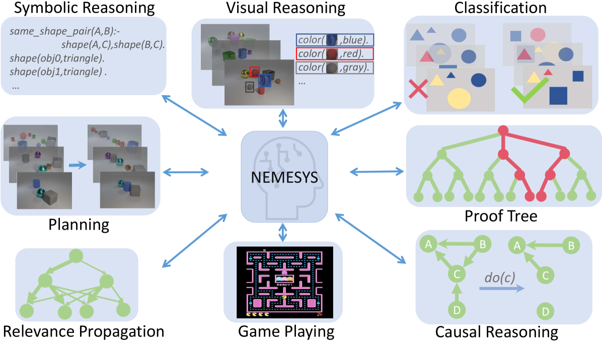
## Diagram: NEMESYS - A Multi-Modal Reasoning System Architecture
### Overview
The image is a conceptual diagram illustrating a central artificial intelligence system named **NEMESYS**, which interacts bidirectionally with eight distinct reasoning or task modules. The diagram is designed to showcase the system's capability to integrate and process diverse types of cognitive and problem-solving tasks. The overall layout features a central hub with eight surrounding modules, each connected to the center by double-headed blue arrows, indicating a two-way flow of information or processing.
### Components/Axes
The diagram is composed of nine primary components arranged in a radial pattern:
1. **Central Hub:**
* **Label:** "NEMESYS"
* **Visual:** A stylized icon of a human head in profile, filled with a light blue color and overlaid with a white circuit board pattern, symbolizing an artificial brain or cognitive architecture.
* **Position:** Center of the image.
2. **Surrounding Modules (8 total):** Each module is contained within a light blue, rounded rectangular box and is connected to the central NEMESYS hub by a blue, double-headed arrow.
* **Top-Left:** **Symbolic Reasoning**
* **Top-Center:** **Visual Reasoning**
* **Top-Right:** **Classification**
* **Right-Center:** **Proof Tree**
* **Bottom-Right:** **Causal Reasoning**
* **Bottom-Center:** **Game Playing**
* **Bottom-Left:** **Relevance Propagation**
* **Left-Center:** **Planning**
### Detailed Analysis / Content Details
Each module contains specific visual and textual content representing its function:
* **Symbolic Reasoning (Top-Left):**
* **Content:** Contains text resembling Prolog or logical programming code.
* **Transcribed Text:**
```
same_shape_pair(A,B):-
shape(A,C),shape(B,C).
shape(obj0,triangle).
shape(obj1,triangle).
...
```
* **Visual Reasoning (Top-Center):**
* **Content:** A composite image showing a 3D scene with various colored objects (spheres, cubes, cylinders) on a surface. Overlaid on the right is a table-like structure with color swatches and labels.
* **Transcribed Text (Table):**
```
color( [blue swatch], blue).
color( [red swatch], red).
color( [gray swatch], gray).
...
```
* **Classification (Top-Right):**
* **Content:** Two panels comparing classification outcomes. The left panel shows various shapes (triangles, circles, squares) with a large red "X" over a yellow triangle, indicating misclassification. The right panel shows similar shapes with a large green checkmark over a yellow triangle, indicating correct classification.
* **Proof Tree (Right-Center):**
* **Content:** A hierarchical tree diagram. The root and some nodes are colored red, while the majority of leaf nodes are green. This likely represents a logical deduction or search tree where red nodes might indicate a failed path or a specific branch of interest, and green nodes indicate successful or explored paths.
* **Causal Reasoning (Bottom-Right):**
* **Content:** A directed acyclic graph (DAG) with nodes labeled A, B, C, D. Arrows show causal relationships (e.g., A -> C, B -> C, C -> D). A separate arrow labeled "do(c)" points from a version of the graph where node C is intervened upon (highlighted), illustrating the concept of causal intervention.
* **Game Playing (Bottom-Center):**
* **Content:** A screenshot from the classic arcade game **Pac-Man**. It shows the game maze, Pac-Man, ghosts, dots, and power pellets.
* **Relevance Propagation (Bottom-Left):**
* **Content:** A network graph with interconnected green nodes. The structure suggests a neural network or a graph where information or "relevance" is propagated between nodes.
* **Planning (Left-Center):**
* **Content:** A sequence of four 3D rendered scenes showing the progressive rearrangement of objects (cubes, spheres) on a surface. An arrow points from the first scene to the last, indicating a plan or sequence of actions to achieve a goal state.
### Key Observations
1. **Bidirectional Integration:** Every module has a direct, two-way connection to the central NEMESYS system, emphasizing that it is not a simple pipeline but an integrated architecture where the core system and specialized modules constantly interact.
2. **Diversity of Tasks:** The diagram explicitly covers a wide spectrum of AI challenges: logical reasoning (Symbolic, Proof Tree), perception (Visual Reasoning, Classification), sequential decision-making (Planning, Game Playing), and relational modeling (Causal Reasoning, Relevance Propagation).
3. **Visual Metaphors:** Each module uses a distinct visual metaphor appropriate to its domain (code for symbolic, 3D scenes for planning/visual, graphs for causal/relevance, a game screenshot for playing).
4. **Color Coding:** The use of color is functional: red/green in Proof Tree and Classification denotes success/failure or different states; the consistent blue of the central hub and arrows unifies the diagram.
### Interpretation
This diagram presents **NEMESYS** as a proposed unified cognitive architecture designed to tackle artificial general intelligence (AGI) by integrating multiple, traditionally separate, AI sub-fields. The central "brain" icon suggests it acts as a central executive or common substrate.
* **What it suggests:** The architecture implies that robust intelligence requires the synergistic combination of different reasoning types. For instance, solving a complex real-world problem might require **Visual Reasoning** to perceive the scene, **Symbolic Reasoning** to represent knowledge, **Causal Reasoning** to understand effects of actions, and **Planning** to devise a solution sequence.
* **How elements relate:** The bidirectional arrows are the most critical relational element. They indicate that NEMESYS both *utilizes* the capabilities of each module (e.g., sending perceptual data to the Classification module) and *informs or trains* them (e.g., using high-level symbolic knowledge to guide visual attention). The modules are not isolated silos but components of a greater whole.
* **Notable Anomalies/Outliers:** The **Game Playing (Pac-Man)** module stands out as a specific, well-defined benchmark environment, whereas the others are more abstract reasoning tasks. This may indicate that the system is validated on both standardized benchmarks and open-ended reasoning problems. The **Proof Tree** and **Relevance Propagation** graphs are visually similar but labeled differently, hinting at a distinction between explicit logical proof search and implicit, possibly neural, information flow.
In essence, the diagram is a blueprint for a holistic AI system, arguing that the path to more general intelligence lies not in perfecting a single algorithm but in architecting a framework where diverse cognitive modules collaborate through a central, integrative core.
</details>
Figure 1: NEMESYS solves different kinds of tasks by using meta-level reasoning and learning. NEMESYS addresses, for instance, visual reasoning, planning, and causal reasoning without modifying its internal reasoning architecture. (Best viewed in color)
## 1 Introduction
One of the distant goals of Artificial Intelligence (AI) is to build a fully autonomous or ‘human-like’ system. The current successes of deep learning systems such as DALLE-2 [1], ChatGPT [2, 3], and Gato [4] have been promoted as bringing the field closer to this goal. However, current systems still require a large number of computations and often solve rather specific tasks. For example, DALLE-2 can generate very high-quality images but cannot play chess or Atari games. In stark contrast, human minds solve a wide range of problems using a small amount of computation and limited experience.
Most importantly, to be considered a major step towards achieving Artificial General Intelligence (AGI), a system must not only be able to perform a variety of tasks, such as Gato [4] playing Atari games, captioning images, chatting, and controlling a real robot arm, but also be self-reflective and able to learn and reason about its own capabilities. This means that it must be able to improve itself and adapt to new situations through self-reflection [5, 6, 7, 8]. Consequently, the study of meta-level architectures such as meta learning [9] and meta-reasoning [7] becomes progressively important. Meta learning [10] is a way to improve the learning algorithm itself [11, 12], i.e., it performs learning at a higher level, or meta-level. Meta-reasoning is a related concept that involves a system being able to think about its own abilities and how it processes information [5, 6]. It involves reflecting on, or introspecting about, the system’s own reasoning processes.
Indeed, meta-reasoning is different from object-centric reasoning, which refers to the system thinking about entities external to itself [13, 14, 15]. Here, the models perform low-level visual perception and reasoning on high-level concepts. Accordingly, there has been a push to make these reasoning systems differentiable [16, 17] along with addressing benchmarks in a visual domain such as CLEVR [18] and Kandinsky patterns [19, 20]. They use object-centric neural networks to perceive objects and perform reasoning using their output. Although this can solve the proposed benchmarks to some extent, the critical question remains unanswered: Is the reasoner able to justify its own operations? Can the same model solve different tasks such as (causal) reasoning, planning, game playing, and much more?
To overcome these limitations, we propose NEMESYS, the first neural meta -symbolic reasoning system. NEMESYS extensively performs meta-level programming on neuro-symbolic systems, and thus it can reason and learn several tasks. This is different from performing object-level deep reasoning and learning, which refers in some way to entities external to the system. NEMESYS is able to reflect or introspect, i.e., to shift from object- to meta-level reasoning and vice versa.
| | Meta Reasoning | Multitask Adaptation | Differentiable Meta Structure Learning |
| --- | --- | --- | --- |
| DeepProbLog [21] | ✗ | ✗ | ✗ |
| NTPs [22] | ✗ | ✗ | ✗ |
| FFSNL [23] | ✗ | ✗ | ✗ |
| $\alpha$ ILP [24] | ✗ | ✗ | ✗ |
| Scallop [25] | ✗ | ✗ | ✗ |
| NeurASP [26] | ✗ | ✗ | ✗ |
| NEMESYS (ours) | ✓ | ✓ | ✓ |
Table 1: Comparisons between NEMESYS and other state-of-the-art Neuro-Symbolic systems. We compare these systems with NEMESYS in three aspects, whether the system performs meta reasoning, can the same system adapt to solve different tasks and is the system capable of differentiable meta level structure learning.
Overall, we make the following contributions:
1. We propose NEMESYS, the first neural meta -symbolic reasoning and learning system that performs differentiable forward reasoning using meta-level programs.
1. To evaluate the ability of NEMESYS, we propose a challenging task, visual concept repairing, where the task is to rearrange objects in visual scenes based on relational logical concepts.
1. We empirically show that NEMESYS can efficiently solve different visual reasoning tasks with meta-level programs, achieving comparable performances with object-level forward reasoners [16, 24] that use specific programs for each task.
1. Moreover, we empirically show that using powerful differentiable meta-level programming, NEMESYS can solve different kinds of tasks that are difficult, if not impossible, for the previous neuro-symbolic systems. In our experiments, NEMESYS provides the function of (i) reasoning with integrated proof generation, i.e., performing differentiable reasoning producing proof trees, (ii) explainable artificial intelligence (XAI), i.e., highlighting the importance of logical atoms given conclusions, (iii) reasoning avoiding infinite loops, i.e., performing differentiable reasoning on programs which cause infinite loops that the previous logic reasoning systems unable to solve, and (iv) differentiable causal reasoning, i.e., performing causal reasoning [27, 28] on a causal Bayesian network using differentiable meta reasoners. To the best of the authors’ knowledge, we propose the first differentiable $\mathtt{do}$ operator. Achieving these functions with object-level reasoners necessitates significant efforts, and in some cases, it may be unattainable. In stark contrast, NEMESYS successfully realized the different useful functions by having different meta-level programs without any modifications of the reasoning function itself.
1. We demonstrate that NEMESYS can perform structure learning on the meta-level, i.e., learning meta programs from examples and adapting itself to solve different tasks automatically by learning efficiently with gradients.
To this end, we will proceed as follows. We first review (differentiable) first-order logic and reasoning. We then derive NEMESYS by introducing differentiable logical meta programming. Before concluding, we illustrate several capabilities of NEMESYS.
## 2 Background
NEMESYS relies on several research areas: first-order logic, logic programming, differentiable reasoning, meta-reasoning and -learning.
First-Order Logic (FOL)/Logic Programming. A term is a constant, a variable, or a term which consists of a function symbol. We denote $n$ -ary predicate ${\tt p}$ by ${\tt p}/(n,[{\tt dt_{1}},\ldots,{\tt dt_{n}}])$ , where ${\tt dt_{i}}$ is the datatype of $i$ -th argument. An atom is a formula ${\tt p(t_{1},\ldots,t_{n})}$ , where ${\tt p}$ is an $n$ -ary predicate symbol and ${\tt t_{1},\ldots,t_{n}}$ are terms. A ground atom or simply a fact is an atom with no variables. A literal is an atom or its negation. A positive literal is an atom. A negative literal is the negation of an atom. A clause is a finite disjunction ( $\lor$ ) of literals. A ground clause is a clause with no variables. A definite clause is a clause with exactly one positive literal. If $A,B_{1},\ldots,B_{n}$ are atoms, then $A\lor\lnot B_{1}\lor\ldots\lor\lnot B_{n}$ is a definite clause. We write definite clauses in the form of $A~{}\mbox{:-}~{}B_{1},\ldots,B_{n}$ . Atom $A$ is called the head, and a set of negative atoms $\{B_{1},\ldots,B_{n}\}$ is called the body. We call definite clauses as clauses for simplicity in this paper.
Differentiable Forward-Chaining Reasoning. The forward-chaining inference is a type of inference in first-order logic to compute logical entailment [29]. The differentiable forward-chaining inference [16, 17] computes the logical entailment in a differentiable manner using tensor-based operations. Many extensions of differentiable forward reasoners have been developed, e.g., reinforcement learning agents using logic to compute the policy function [30, 31] and differentiable rule learners in complex visual scenes [24]. NEMESYS performs differentiable meta-level logic programming based on differentiable forward reasoners.
<details>
<summary>x2.png Details</summary>
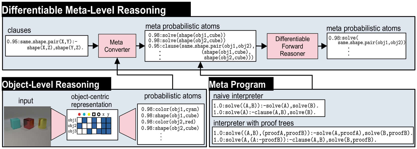
### Visual Description
## Diagram: Differentiable Meta-Level Reasoning and Object-Level Reasoning System
### Overview
This diagram illustrates a two-tiered reasoning system that combines **Object-Level Reasoning** with **Differentiable Meta-Level Reasoning**. The system processes visual input (objects) into symbolic probabilistic atoms, which are then used by a meta-reasoning layer to perform logical inference in a differentiable manner. The flow shows how raw input is transformed into structured knowledge and then reasoned over using a meta-program.
### Components/Axes
The diagram is divided into three primary, interconnected blocks:
1. **Differentiable Meta-Level Reasoning (Top Block):**
* **Input:** `clauses` (e.g., `0.95:same_shape_pair(X,Y):- shape(X,Z),shape(Y,Z).`)
* **Component 1:** `Meta Converter` (pink box).
* **Intermediate Output:** `meta probabilistic atoms` (e.g., `0.98:solve(shape(obj1,cube))`, `0.95:clause(same_shape_pair(obj1,obj2), (shape(obj1,cube), shape(obj2,cube)))`).
* **Component 2:** `Differentiable Forward Reasoner` (pink box).
* **Final Output:** `meta probabilistic atoms` (e.g., `0.98:solve(same_shape_pair(obj1,obj2))`).
2. **Object-Level Reasoning (Bottom-Left Block):**
* **Input:** `input` - A photograph showing three 3D objects: a cyan cube, a red cube, and a yellow cylinder.
* **Component 1:** `object-centric representation` - A schematic grid with rows labeled `obj1`, `obj2`, `obj3` and columns with icons for color (red, cyan, yellow dots), shape (square, circle), and spatial coordinates (`x`, `y`). The grid contains blue and white cells indicating feature presence/absence.
* **Output:** `probabilistic atoms` (e.g., `0.98:color(obj1,cyan)`, `0.98:shape(obj1,cube)`, `0.98:color(obj2,red)`, `0.98:shape(obj2,cube)`).
3. **Meta Program (Bottom-Right Block):**
* This block defines the logical rules for the reasoning system.
* **Sub-component 1:** `naive interpreter`
* Rule 1: `1.0:solve((A,B)):-solve(A),solve(B).`
* Rule 2: `1.0:solve(A):-clause(A,B),solve(B).`
* **Sub-component 2:** `interpreter with proof trees`
* Rule 1: `1.0:solve((A,B),(proofA,proofB)):-solve(A,proofA),solve(B,proofB).`
* Rule 2: `1.0:solve(A,(A:-proofB)):-clause(A,B),solve(B,proofB).`
**Flow and Connections:**
* The `probabilistic atoms` from the **Object-Level Reasoning** block feed into the `Meta Converter` in the **Differentiable Meta-Level Reasoning** block.
* The `Meta Program` block provides the logical rules that govern the `Meta Converter` and the `Differentiable Forward Reasoner`.
* The overall data flow is: **Input Image** -> **Object-Centric Representation** -> **Probabilistic Atoms** -> **Meta Converter** -> **Meta Probabilistic Atoms** -> **Differentiable Forward Reasoner** -> **Inferred Meta Probabilistic Atoms**.
### Detailed Analysis
**Text Transcription and Structure:**
* **Title:** `Differentiable Meta-Level Reasoning` (Top-left, white text on black background).
* **Object-Level Reasoning Title:** `Object-Level Reasoning` (Bottom-left, white text on black background).
* **Meta Program Title:** `Meta Program` (Bottom-right, white text on black background).
* **Clause Example:** `0.95:same_shape_pair(X,Y):- shape(X,Z),shape(Y,Z).` This is a probabilistic logic rule with a confidence of 0.95.
* **Meta Probabilistic Atoms (Input to Reasoner):**
* `0.98:solve(shape(obj1,cube))`
* `0.98:solve(shape(obj2,cube))`
* `0.95:clause(same_shape_pair(obj1,obj2), (shape(obj1,cube), shape(obj2,cube)))`
* **Meta Probabilistic Atoms (Output of Reasoner):**
* `0.98:solve(same_shape_pair(obj1,obj2))`
* **Probabilistic Atoms (from Object-Level):**
* `0.98:color(obj1,cyan)`
* `0.98:shape(obj1,cube)`
* `0.98:color(obj2,red)`
* `0.98:shape(obj2,cube)`
* **Meta Program Rules:** (As transcribed in the Components section above).
### Key Observations
1. **Hierarchical Abstraction:** The system clearly separates low-level perception (Object-Level) from high-level logical reasoning (Meta-Level).
2. **Probabilistic Foundation:** All knowledge is represented with confidence scores (e.g., 0.98, 0.95), indicating a probabilistic logic framework.
3. **Differentiable Pipeline:** The presence of a "Differentiable Forward Reasoner" suggests the entire reasoning chain is designed to be trained end-to-end using gradient-based methods.
4. **Symbolic Grounding:** The `object-centric representation` bridges the gap between continuous visual data and discrete symbolic atoms (`obj1`, `cube`, `cyan`).
5. **Meta-Interpretation:** The `Meta Program` contains interpreters that define how logical deduction (`solve`) operates, with the "proof trees" version providing a more detailed trace of the reasoning process.
### Interpretation
This diagram represents a neuro-symbolic AI architecture. Its purpose is to perform **explainable, logical reasoning over perceptual data** in a way that is compatible with modern deep learning.
* **What it demonstrates:** The system can take an image of objects, identify their properties (color, shape) with high confidence, and then use logical rules to infer higher-order relationships (e.g., "these two objects have the same shape"). The "differentiable" aspect means the system can potentially learn these rules or the perception module from data.
* **Relationships:** The Object-Level module acts as a **perceptual front-end**, grounding symbols in sensory input. The Meta-Level module acts as a **logical reasoning engine**, manipulating these symbols according to a programmable `Meta Program`. The `Meta Converter` is the crucial translator that formats grounded facts into a structure suitable for meta-reasoning.
* **Significance:** This architecture addresses a key challenge in AI: combining the robust pattern recognition of neural networks with the explicit, interpretable reasoning of symbolic logic. The use of probabilities and differentiability makes it trainable and robust to perceptual uncertainty. The output (`solve(same_shape_pair(obj1,obj2))`) is not just a prediction but a **logical conclusion** derived from a traceable chain of evidence and rules.
</details>
Figure 2: Overview of NEMESYS together with an object-level reasoning layer (bottom left). The meta-level reasoner (top) takes a logic program as input, here clauses on the left-hand side in the meta-level reasoning pipeline. Using the meta program (bottom right) it can realize the standard Prolog engine (naive interpreter) or an interpreter that provides e.g., also the proof trees (interpreter with proof trees) without requiring any alterations to the original logic program and internal reasoning function. This means that NEMESYS can integrate many useful functionalities by simply changing devised meta programs without intervening the internal reasoning function. (Best viewed in color)
Meta Reasoning and Learning. Meta-reasoning is the study about systems which are able to reason about its operation, i.e., a system capable of meta-reasoning may be able to reflect, or introspect [32], shifting from meta-reasoning to object-level reasoning and vice versa [6, 7]. Compared with imperative programming, it is relatively easier to construct a meta-interpreter using declarative programming. First-order Logic [33] has been the major tool to realize the meta-reasoning systems [34, 35, 36]. For example, Prolog [37] provides very efficient implementations of meta-interpreters realizing different additional features to the language.
Despite early interest in meta-reasoning within classical Inductive Logic Programming (ILP) systems [38, 39, 40], meta-interpreters have remained unexplored within neuro-symbolic AI. Meta-interpreters within classical logic are difficult to be combined with gradient-based machine learning paradigms, e.g., deep neural networks. NEMESYS realizes meta-level reasoning using differentiable forward reasoners in first-order logic, which are able to perform differentiable rule learning on complex visual scenes with deep neural networks [24]. Moreover, NEMESYS paves the way to integrate meta-level reasoning into other neuro-symbolic frameworks, including DeepProbLog [21], Scallop [25] and NeurASP [26], which are rather developed for training neural networks given logic programs using differentiable backward reasoning or answer set semantics. We compare NEMESYS with several popular neuro-symbolic systems in three aspects: whether the system performs meta reasoning, can the same system adapt to solve different tasks and is the system capable of differentiable meta level structure learning. The comparison results are summarized in Table 1.
## 3 Neural Meta-Symbolic Reasoning & Learning
We now introduce NEMESYS, the first neural meta-symbolic reasoning and learning framework. Fig. 2 shows an overview of NEMESYS.
### 3.1 Meta Logic Programming
We describe how meta-level programs are used in the NEMESYS workflow. In Fig. 2, the following object-level clause is given as its input:
| | $\displaystyle\mathtt{\color[rgb]{0,0.6,0}same\_shape\_pair(X,Y)\color[rgb]{ 0,0,0}\texttt{:-}\color[rgb]{0.68,0.36,1}shape(X,Z),shape(Y,Z)\color[rgb]{ 0,0,0}.}$ | |
| --- | --- | --- |
which identifies pairs of objects that have the same shape. The clause is subsequently fed to Meta Converter, which generates meta-level atoms.Using meta predicate $\mathtt{clause}/2$ , the following atom is generated:
| | $\displaystyle\mathtt{clause(\color[rgb]{0,0.6,0}same\_shape\_pair(X,Y),}\color [rgb]{0.68,0.36,1}\mathtt{(shape(X,Z),shape(Y,Z))\color[rgb]{0,0,0}).}$ | |
| --- | --- | --- |
where the meta atom $\mathtt{clause(H,B)}$ represents the object-level clause: $\mathtt{H\texttt{:-}B}$ .
To perform meta-level reasoning, NEMESYS uses meta-level programs, which often refer to meta interpreters, i.e., interpreters written in the language itself, as illustrated in Fig. 2. For example, a naive interpreter, NaiveInterpreter, is defined as:
| | $\displaystyle\mathtt{solve(true)}.$ | |
| --- | --- | --- |
To solve a compound goal $\mathtt{(A,B)}$ , we need first solve $\mathtt{A}$ and then $\mathtt{B}$ . A single goal $\mathtt{A}$ is solved if there is a clause that rewrites the goal to the new goal $\mathtt{B}$ , the body of the clause: $\mathtt{\color[rgb]{0,0.6,0}{A}\texttt{:-}\color[rgb]{0.68,0.36,1}{B}}$ . This process stops for facts, encoded as $\mathtt{clause(fact,true)}$ , since then, $\mathtt{solve(true)}$ will be true.
NEMESYS can employ more enriched meta programs with useful functions by simply changing the meta programs, without modifying the internal reasoning function, as illustrated in the bottom right of Fig. 2. ProofTreeInterpreter, an interpreter that produces proof trees along with reasoning, is defined as:
| | $\displaystyle\mathtt{solve(A,(A\texttt{:-}true)).}$ | |
| --- | --- | --- |
where $\mathtt{solve(A,Proof)}$ checks if atom $\mathtt{A}$ is true with proof tree $\mathtt{Proof}$ . Using this meta-program, NEMESYS can perform reasoning with integrated proof tree generation.
Now, let us devise the differentiable meta-level reasoning pipeline, which enables NEMESYS to reason and learn flexibly.
### 3.2 Differentiable Meta Programming
NEMESYS employs differentiable forward reasoning [24], which computes logical entailment using tensor operations in a differentiable manner, by adapting it to the meta-level atoms and clauses.
We define a meta-level reasoning function $f^{\mathit{reason}}_{(\mathcal{C},\mathbf{W})}:[0,1]^{G}\rightarrow[0,1]^{G}$ parameterized by meta-rules $\mathcal{C}$ and their weights $\mathbf{W}$ . We denote the set of meta-rules by $\mathcal{C}$ , and the set of all of the meta-ground atoms by $\mathcal{G}$ . $\mathcal{G}$ contains all of the meta-ground atoms produced by a given FOL language. We consider ordered sets here, i.e., each element has its index. We denote the size of the sets as: $G=|\mathcal{G}|$ and $C=|\mathcal{C}|$ . We denote the $i$ -th element of vector $\mathbf{x}$ by $\mathbf{x}[i]$ , and the $(i,j)$ -th element of matrix $\mathbf{X}$ by $\mathbf{X}[i,j]$ .
First, NEMESYS converts visual input to a valuation vector $\mathbf{v}\in[0,1]^{G}$ , which maps each meta atom to a probabilistic value (Fig. 2 Meta Converter). For example,
$$
\mathbf{v}=\blockarray{cl}\block{[c]l}0.98&\mathtt{solve(color(obj1,\ cyan))}
\\
0.01\mathtt{solve(color(obj1,\ red))}\\
0.95\mathtt{clause(same\_shape\_pair(\ldots),\ (shape(\ldots),\ \ldots))}\\
$$
represents a valuation vector that maps each meta-ground atom to a probabilistic value. For readability, only selected atoms are shown. NEMESYS computes logical entailment by updating the initial valuation vector $\mathbf{v}^{(0)}$ for $T$ times to $\mathbf{v}^{(T)}$ .
Subsequently, we compose the reasoning function that computes logical entailment. We now describe each step in detail.
(Step 1) Encode Logic Programs to Tensors.
To achieve differentiable forward reasoning, each meta-rule is encoded to a tensor representation. Let $S$ be the maximum number of substitutions for existentially quantified variables in $\mathcal{C}$ , and $L$ be the maximum length of the body of rules in $\mathcal{C}$ . Each meta-rule $C_{i}\in\mathcal{C}$ is encoded to a tensor ${\bf I}_{i}\in\mathbb{N}^{G\times S\times L}$ , which contains the indices of body atoms. Intuitively, $\mathbf{I}_{i}[j,k,l]$ is the index of the $l$ -th fact (subgoal) in the body of the $i$ -th rule to derive the $j$ -th fact with the $k$ -th substitution for existentially quantified variables. We obtain $\mathbf{I}_{i}$ by firstly grounding the meta rule $C_{i}$ , then computing the indices of the ground body atoms, and transforming them into a tensor.
(Step 2) Assign Meta-Rule Weights.
We assign weights to compose the reasoning function with several meta-rules as follows: (i) We fix the target programs’ size as $M$ , i.e., we try to select a meta-program with $M$ meta-rules out of $C$ candidate meta rules. (ii) We introduce $C$ -dimensional weights $\mathbf{W}=[{\bf w}_{1},\ldots,{\bf w}_{M}]$ where $\mathbf{w}_{i}\in\mathbb{R}^{C}$ . (iii) We take the softmax of each weight vector ${\bf w}_{j}\in\mathbf{W}$ and softly choose $M$ meta rules out of $C$ meta rules to compose the differentiable meta program.
(Step 3) Perform Differentiable Inference.
We compute $1$ -step forward reasoning using weighted meta-rules, then we recursively perform reasoning to compute $T$ -step reasoning.
(i) Reasoning using one rule. First, for each meta-rule $C_{i}\in\mathcal{C}$ , we evaluate body atoms for different grounding of $C_{i}$ by computing:
$$
\displaystyle b_{i,j,k}^{(t)}=\prod_{1\leq l\leq L}{\bf gather}({\bf v}^{(t)},
{\bf I}_{i})[j,k,l], \tag{1}
$$
where $\mathbf{gather}:[0,1]^{G}\times\mathbb{N}^{G\times S\times L}\rightarrow[0,1]^ {G\times S\times L}$ is:
$$
\displaystyle\mathbf{gather}({\bf x},{\bf Y})[j,k,l]={\bf x}[{\bf Y}[j,k,l]], \tag{2}
$$
and $b^{(t)}_{i,j,k}\in[0,1]$ . The $\mathbf{gather}$ function replaces the indices of the body atoms by the current valuation values in $\mathbf{v}^{(t)}$ . To take logical and across the subgoals in the body, we take the product across valuations. $b_{i,j,k}^{(t)}$ represents the valuation of body atoms for $i$ -th meta-rule using $k$ -th substitution for the existentially quantified variables to deduce $j$ -th meta-ground atom at time $t$ .
Now we take logical or softly to combine all of the different grounding for $C_{i}$ by computing $c^{(t)}_{i,j}\in[0,1]$ :
$$
\displaystyle c^{(t)}_{i,j}=\mathit{softor}^{\gamma}(b_{i,j,1}^{(t)},\ldots,b_
{i,j,S}^{(t)}), \tag{3}
$$
where $\mathit{softor}^{\gamma}$ is a smooth logical or function:
$$
\displaystyle\mathit{softor}^{\gamma}(x_{1},\ldots,x_{n})=\gamma\log\sum_{1
\leq i\leq n}\exp(x_{i}/\gamma), \tag{4}
$$
where $\gamma>0$ is a smooth parameter. Eq. 4 is an approximation of the max function over probabilistic values based on the log-sum-exp approach [41].
(ii) Combine results from different rules. Now we apply different meta-rules using the assigned weights by computing:
$$
\displaystyle h_{j,m}^{(t)}=\sum_{1\leq i\leq C}w^{*}_{m,i}\cdot c_{i,j}^{(t)}, \tag{5}
$$
where $h_{j,m}^{(t)}\in[0,1]$ , $w^{*}_{m,i}=\exp(w_{m,i})/{\sum_{i^{\prime}}\exp(w_{m,i^{\prime}})}$ , and $w_{m,i}=\mathbf{w}_{m}[i]$ . Note that $w^{*}_{m,i}$ is interpreted as a probability that meta-rule $C_{i}\in\mathcal{C}$ is the $m$ -th component. We complete the $1$ -step forward reasoning by combining the results from different weights:
$$
\displaystyle r_{j}^{(t)}=\mathit{softor}^{\gamma}(h_{j,1}^{(t)},\ldots,h_{j,M
}^{(t)}). \tag{6}
$$
Taking $\mathit{softor}^{\gamma}$ means that we compose $M$ softly chosen rules out of $C$ candidate meta-rules.
(iii) Multi-step reasoning. We perform $T$ -step forward reasoning by computing $r_{j}^{(t)}$ recursively for $T$ times: $v^{(t+1)}_{j}=\mathit{softor}^{\gamma}(r^{(t)}_{j},v^{(t)}_{j})$ . Updating the valuation vector for $T$ -times corresponds to computing logical entailment softly by $T$ -step forward reasoning. The whole reasoning computation Eq. 1 - 6 can be implemented using efficient tensor operations.
## 4 Experiments
With the methodology of NEMESYS established, we subsequently provide empirical evidence of its benefits over neural baselines and object-level neuro-symbolic approaches: (1) NEMESYS can emulate a differentiable forward reasoner, i.e., it is a sufficient implementation of object-centric reasoners with a naive meta program. (2) NEMESYS is capable of differentiable meta-level reasoning, i.e., it can integrate additional useful functions using devised meta-rules. We demonstrate this advantage by solving tasks of proof-tree generation, relevance propagation, automated planning, and causal reasoning. (3) NEMESYS can perform parameter and structure learning efficiently using gradient descent, i.e., it can perform learning on meta-level programs.
In our experiments, we implemented NEMESYS in Python using PyTorch, with CPU: intel i7-10750H and RAM: 16 GB.
| | NEMESYS | ResNet50 | YOLO+MLP |
| --- | --- | --- | --- |
| Twopairs | 100.0 $\bullet$ | 50.81 | 98.07 $\circ$ |
| Threepairs | 100.0 $\bullet$ | 51.65 | 91.27 $\circ$ |
| Closeby | 100.0 $\bullet$ | 54.53 | 91.40 $\circ$ |
| Red-Triangle | 95.6 $\bullet$ | 57.19 | 78.37 $\circ$ |
| Online/Pair | 100.0 $\bullet$ | 51.86 | 66.19 $\circ$ |
| 9-Circles | 95.2 $\bullet$ | 50.76 $\circ$ | 50.76 $\circ$ |
Table 2: Performance (accuracy; the higher, the better) on the test split of Kandinsky patterns. The best-performing models are denoted using $\bullet$ , and the runner-up using $\circ$ . In Kandinsky patterns, NEMESYS produced almost perfect accuracies outperforming neural baselines, where YOLO+MLP is a neural baseline using pre-trained YOLO [42] combined with a simple MLP, showing the capability of solving complex visual reasoning tasks. The performances of baselines are shown in [15].
### 4.1 Visual Reasoning on Complex Pattenrs
Let us start off by showing that our NEMESYS is able to obtain the equivalent high-quality results as a standard object-level reasoner but on the meta-level. We considered tasks of Kandinsky patterns [19, 43] and CLEVR-Hans [14] We refer to [14] and [15] for detailed explanations of the used patterns for CLEVR-Hans and Kandinsky patterns.. CLEVR-Hans is a classification task of complex 3D visual scenes. We compared NEMESYS with the naive interpreter against neural baselines and a neuro-symbolic baseline, $\alpha$ ILP [24], which achieves state-of-the-art performance on these tasks. For all tasks, NEMESYS achieved exactly the same performances with $\alpha$ ILP since the naive interpreter realizes a conventional object-centric reasoner. Moreover, as shown in Table 2 and Table 3, NEMESYS outperformed neural baselines on each task. This shows that NEMESYS is able to solve complex visual reasoning tasks using meta-level reasoning without sacrificing performance.
In contrast to the object-centric reasoners, e.g., $\alpha$ ILP. NEMESYS can easily integrate additional useful functions by simply switching or adding meta programs without modifying the internal reasoning function, as shown in the next experiments.
### 4.2 Explainable Logical Reasoning
One of the major limitations of differentiable forward chaining [16, 17, 24] is that they lack the ability to explain the reasoning steps and their evidence. We show that NEMESYS achieves explainable reasoning by incorporating devised meta-level programs.
Reasoning with Integrated Proof Tree Generation
First, we demonstrate that NEMESYS can generate proof trees while performing reasoning, which the previous differentiable forward reasoners cannot produce since they encode the reasoning function to computational graphs using tensor operations and observe only their input and output. Since NEMESYS performs reasoning using meta-level programs, it can add the function to produce proof trees into its underlying reasoning mechanism simply by devising them, as illustrated in Fig 2.
We use Kandinsky patterns [20], a benchmark of visual reasoning whose classification rule is defined on high-level concepts of relations and attributes of objects. We illustrate the input on the top right of Fig. 3 that belongs to a pattern: ”There are two pairs of objects that share the same shape.” Given the visual input, proof trees generated using the ProofTreeInterpreter in Sec. 3.1 are shown on the left two boxes of Fig. 3. In this experiment, NEMESYS identified the relations between objects, and the generated proof trees explain the intermediate reasoning steps.
<details>
<summary>x3.png Details</summary>
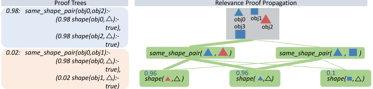
### Visual Description
## Diagram: Proof Trees and Relevance Proof Propagation
### Overview
The image is a technical diagram illustrating a logical reasoning process. It is divided into two main panels: "Proof Trees" on the left and "Relevance Proof Propagation" on the right. The diagram visualizes how confidence scores (probabilities) are assigned to logical statements about object shapes and how these proofs propagate through a network to establish relationships between objects.
### Components/Axes
The diagram has no traditional chart axes. Its components are:
**Left Panel: Proof Trees**
* **Title:** "Proof Trees" (centered at the top of the left panel).
* **Content:** Two distinct proof trees, each presented in a colored box.
* **Top Box (Light Blue):** Contains a logical proof with a confidence score of `0.98`.
* **Bottom Box (Light Orange):** Contains a logical proof with a confidence score of `0.02`.
**Right Panel: Relevance Proof Propagation**
* **Title:** "Relevance Proof Propagation" (centered at the top of the right panel).
* **Object Legend (Top Center):** A grey box containing four labeled objects with associated shapes and colors:
* `obj0`: Blue triangle (▲)
* `obj1`: Blue square (■)
* `obj2`: Red triangle (▲)
* `obj3`: Blue square (■)
* **Propagation Network:** A hierarchical network of green nodes connected by green lines, showing the flow of logical inference.
* **Top Layer Nodes:** Two nodes representing `same_shape_pair` relationships.
* **Bottom Layer Nodes:** Three nodes representing `shape` properties of individual objects.
### Detailed Analysis
**1. Proof Trees (Left Panel)**
* **Proof 1 (Confidence: 0.98):**
* **Statement:** `same_shape_pair(obj0, obj2)`
* **Derivation:** This is proven by two sub-statements, both with confidence `0.98`:
* `shape(obj0, △)` is `true`.
* `shape(obj2, △)` is `true`.
* **Interpretation:** There is a 98% confidence that `obj0` and `obj2` are a pair of the same shape because both are confidently identified as triangles.
* **Proof 2 (Confidence: 0.02):**
* **Statement:** `same_shape_pair(obj0, obj1)`
* **Derivation:** This is derived from two sub-statements with conflicting confidences:
* `shape(obj0, △)` is `true` (confidence: `0.98`).
* `shape(obj1, △)` is `true` (confidence: `0.02`).
* **Interpretation:** There is only a 2% confidence that `obj0` and `obj1` are a same-shape pair. This low confidence stems from the very low confidence (`0.02`) that `obj1` is a triangle, which contradicts the visual legend showing `obj1` as a square.
**2. Relevance Proof Propagation (Right Panel)**
* **Object Legend:** Establishes the ground truth for the example:
* `obj0` = Blue Triangle
* `obj1` = Blue Square
* `obj2` = Red Triangle
* `obj3` = Blue Square
* **Propagation Network Nodes & Values:**
* **Top-Left Node:** `same_shape_pair(▲, ▲)` (Blue Triangle, Red Triangle). This corresponds to the pair (`obj0`, `obj2`).
* **Top-Right Node:** `same_shape_pair(▲, ■)` (Blue Triangle, Blue Square). This corresponds to the pair (`obj0`, `obj1`) or (`obj0`, `obj3`).
* **Bottom-Left Node:** `shape(▲, △)` with confidence `0.96`. This represents the property that a red triangle is a triangle.
* **Bottom-Center Node:** `shape(▲, △)` with confidence `0.96`. This represents the property that a blue triangle is a triangle.
* **Bottom-Right Node:** `shape(■, △)` with confidence `0.1`. This represents the (low confidence) property that a blue square is a triangle.
* **Flow and Connections:**
* The `same_shape_pair(▲, ▲)` node is connected to the two `shape(▲, △)` nodes (both confidence `0.96`). This visually represents the proof logic from the left panel: the high-confidence pair relationship is supported by high-confidence individual shape properties.
* The `same_shape_pair(▲, ■)` node is connected to one `shape(▲, △)` node (confidence `0.96`) and the `shape(■, △)` node (confidence `0.1`). This represents the low-confidence pair relationship being supported by one high-confidence and one low-confidence shape property.
### Key Observations
1. **Confidence Alignment:** The confidence scores in the Proof Trees (`0.98`, `0.02`) are closely mirrored by the propagated scores in the network (`0.96`, `0.1`). The minor discrepancy (0.98 vs 0.96) may be due to rounding or a slightly different calculation in the propagation step.
2. **Visual-Logical Consistency:** The diagram highlights a conflict. The object legend clearly shows `obj1` is a square, yet the low-confidence proof (`0.02`) attempts to assert it is a triangle. The propagation network correctly assigns a low confidence (`0.1`) to the statement `shape(■, △)`.
3. **Spatial Grounding:** The legend is positioned at the top-center of the right panel, providing the key to interpreting all shape symbols and colors in the network below. The proof trees are isolated on the left, providing the formal logical statements that the right panel visualizes.
4. **Color Coding:** Colors are used consistently: blue and red for object triangles, blue for squares, green for the propagation network, and distinct background colors (blue/orange) to separate high and low-confidence proofs.
### Interpretation
This diagram demonstrates a **probabilistic logical reasoning system**. It shows how a system can:
* **Generate Hypotheses:** Formulate logical statements (proofs) about relationships (`same_shape_pair`) based on object properties (`shape`).
* **Assign Confidence:** Attach numerical confidence scores to these statements, reflecting uncertainty in perception or reasoning.
* **Propagate Relevance:** Visualize how the confidence in a high-level relationship (like "these two objects have the same shape") is fundamentally dependent on and derived from the confidence in the lower-level properties of the individual objects involved.
The core message is that the strength of a logical conclusion is only as strong as its weakest premise. The high-confidence conclusion that `obj0` and `obj2` are both triangles is robust. In contrast, the attempt to conclude `obj0` and `obj1` are the same shape fails because the premise that `obj1` is a triangle has very low confidence, correctly reflecting the visual evidence that `obj1` is a square. This type of reasoning is crucial in fields like artificial intelligence, computer vision, and knowledge graphs, where systems must handle uncertainty and infer relationships from imperfect data.
</details>
Figure 3: NEMESYS explains its reasoning with proof trees and relevance proof propagation. Given the image involving four objects (top, right), NEMESYS provides two proofs (two boxes on the left, true atom’s proof (blue box) and false atom’s proof (cream box)). They can be leveraged to decompose the prediction of NEMESYS into relevance scores per (ground) atom (right). First, a standard forward reasoning is performed to compute the prediction. Then, the model’s prediction is backward propagated through the proof trees by applying specific decomposition rules, see main text. The numbers next to each (ground) atom are the relevance scores computed. The larger the score is, the more impact an (ground) atom has on the final prediction, and the line width is wider. For brevity, the complete proof tree is not depicted here. As our baseline comparison, we extend DeepProbLog [21] to DeepMetaProbLog. However, DeepMetaProbLog only provides proof tree for true atoms (top left blue box). (Best viewed in color)
| | CLEVR-Hans3 | CLEVR-Hans7 | | |
| --- | --- | --- | --- | --- |
| Validation | Test | Validation | Test | |
| CNN | 99.55 $\circ$ | 70.34 | 96.09 | 84.50 |
| NeSy (Default) | 98.55 | 81.71 | 96.88 $\circ$ | 90.97 |
| NeSy-XIL | 100.00 $\bullet$ | 91.31 $\circ$ | 98.76 $\bullet$ | 94.96 $\bullet$ |
| NEMESYS | 98.18 | 98.40 $\bullet$ | 93.60 | 92.19 $\circ$ |
Table 3: Performance (accuracy; the higher, the better) on the validation/test splits of 3D CLEVR-Hans data sets. The best-performing models are denoted using $\bullet$ , and the runner-up using $\circ$ . In CLEVR-Hans, NEMESYS outperformed neural baselines including: (CNN) A ResNet [44], (NeSy) A model combining object-centric model (Slot Attention [45] and Set Transformer [46], and (NeSy-XIL) Slot Attention and Set Transformer using human feedback. NEMESYS tends to show less overfitting and performs similarly to a neuro-symbolic approach using human feedback (NeSy-XIL). The performances of baselines are shown in [14] and [15].
Let’s first consider the top left blue box depicted in Fig. 3 (for readability, we only show the proof part of meta atoms in the image). The weighted ground atom $\mathtt{0.98:}\mathtt{same\_shape\_pair(obj0,obj2)}$ proves $\mathtt{obj0}$ and $\mathtt{obj2}$ are of the same shape with the probability $0.98$ . The proof part shows that NEMESYS comes to this conclusion since both objects are triangle with probabilities of $\mathtt{0.98}$ and in turn it can apply the rule for $\mathtt{same\_shape\_pair}$ . We use this example to show how to compute the weight of the meta atoms inside NEMESYS. With the proof-tree meta rules and corresponding meta ground atoms:
| | $\displaystyle\mathtt{0.98:}\ \color[rgb]{0.5,0,1}\mathtt{solve(shape(obj0,} \text{\includegraphics[height=6.45831pt]{plots/triangle.png}}\mathtt{),(shape( obj0,}\text{\includegraphics[height=6.45831pt]{plots/triangle.png}}\mathtt{), true).}$ | |
| --- | --- | --- |
The weight of the meta ground atoms are computed by Meta Converter when mapping the probability of meta ground atoms to a continuous value. The meta ground atom says that $\mathtt{shape(obj0,\includegraphics[height=6.45831pt]{plots/triangle.png})}$ is true with a high probability of $0.98$ because $\mathtt{shape(obj0,\includegraphics[height=6.45831pt]{plots/triangle.png})}$ can be proven.
With the two meta ground atoms at hand, we infer the weight of the meta atom with compound goals $\color[rgb]{0,0.6,0}\mathtt{solve((shape(obj0,\includegraphics[height=6.45831 pt]{plots/triangle.png}),shape(obj2,\includegraphics[height=6.45831pt]{plots/ triangle.png})),(ProofA,ProofB))}$ , based on the first meta rule (for readability, we omit writing out the proof part). Then, we use the second meta rule to compute the weight of the meta atom $\color[rgb]{0.68,0.36,1}\mathtt{solve}\mathtt{(same\_shape\_pair(obj0,obj2)}, \mathtt{(Proof))}$ , using the compound goal meta atom $\color[rgb]{0,0.6,0}\mathtt{solve((shape(obj0,\includegraphics[height=6.45831 pt]{plots/triangle.png}),shape(obj2,\includegraphics[height=6.45831pt]{plots/ triangle.png})),(ProofA,ProofB))}$ and the meta atom $\mathtt{clause}\mathtt{(same\_shape\_pair(obj0,obj2)},\mathtt{(shape(obj0, \includegraphics[height=6.45831pt]{plots/triangle.png})},\mathtt{shape(obj2, \includegraphics[height=6.45831pt]{plots/triangle.png})))}$ .
In contrast, NEMESYS can explicitly show that $\mathtt{obj0}$ and $\mathtt{obj1}$ have a low probability of being of the same shape (Fig. 3 left bottom cream box). This proof tree shows that the goal $\mathtt{shape(obj1,\includegraphics[height=6.45831pt]{plots/triangle.png})}$ has a low probability of being true. Thus, as one can read off, $\mathtt{obj0}$ is most likely a triangle, while $\mathtt{obj1}$ is most likely not a triangle. In turn, NEMESYS concludes with a low probability that $\mathtt{same\_shape\_pair(obj0,obj1)}$ is true, only a probability of $0.02$ . NEMESYS can produce all the information required to explain its decisions by simply changing the meta-program, not the underlying reasoning system.
Using meta programming to extend DeepProbLog to produce proof trees as a baseline comparison. Since DeepProbLog [21] doesn’t support generating proof trees in parallel with reasoning, we extend DeepProbLog [21] to DeepMetaProblog to generate proof trees as our baseline comparison using ProbLog [47]. However, the proof tree generated by DeepMetaProbLog is limited to the ‘true’ atoms (Fig. 3 top left blue box), i.e., DeepMetaProbLog is unable to generate proof tree for false atoms such as $\mathtt{same\_shape\_pair(obj0,obj1)}$ (Fig. 3 bottom left cream box) due to backward reasoning.
Logical Relevance Proof Propagation (LRP ${}^{2}$ )
Inspired by layer-wise relevance propagation (LRP) [48], which produces explanations for feed-forward neural networks, we now show that, LRP can be adapted to logical reasoning systems using declarative languages in NEMESYS, thereby enabling the reasoning system to articulate the rationale behind its decisions, i.e., it can compute the importance of ground atoms for a query by having access to proof trees. We call this process: logical relevance proof propagation (LRP ${}^{2}$ ).
The original LRP technique decomposes the prediction of the network, $f(\mathbf{x})$ , onto the input variables, $\mathbf{x}=\left(x_{1},\ldots,x_{d}\right)$ , through a decomposition $\mathbf{R}=\left(R_{1},\ldots,R_{d}\right)$ such that $\sum\nolimits_{p=1}^{d}R_{p}=f(\mathbf{x})\;$ . Given the activation $a_{j}=\rho\left(\sum_{i}a_{i}w_{ij}+b_{j}\right)$ of neuron, where $i$ and $j$ denote the neuron indices at consecutive layers, and $\sum_{i}$ and $\sum_{j}$ represent the summation over all neurons in the respective layers, the propagation of LRP is defined as: $R_{i}=\sum\nolimits_{j}z_{ij}({\sum\nolimits_{i}z_{ij}})^{-1}R_{j},$ where $z_{ij}$ is the contribution of neuron $i$ to the activation $a_{j}$ , typically some function of activation $a_{i}$ and the weight $w_{ij}$ . Starting from the output $f(\mathbf{x})$ , the relevance is computed layer by layer until the input variables are reached.
To adapt this in NEMESYS to ground atoms and proof trees, we have to be a bit careful, since we cannot deal with the uncountable, infinite real numbers within our logic. Fortunately, we can make use of the weight associated with ground atoms. That is, our LRP ${}^{2}$ composes meta-level atoms that represent the relevance of an atom given proof trees and associates the relevance scores to the weights of the meta-level atoms.
To this end, we introduce three meta predicates: $\mathtt{rp/3/[goal,proofs,atom]}$ that represents the relevance score an $\mathtt{atom}$ has on the $\mathtt{goal}$ in given $\mathtt{proofs}$ , $\mathtt{assert\_probs/1/[atom]}$ that looks up the valuations of the ground atoms and maps the probability of the $\mathtt{atom}$ to its weight. $\mathtt{rpf/2/[proof,atom]}$ represents how much an $\mathtt{atom}$ contributes to the $\mathtt{proof}$ . The atom $\mathtt{assert\_probs((Goal\texttt{:-}Body))}$ asserts the probability of the atom $\mathtt{(Goal\texttt{:-}Body)}$ . With them, the meta-level program of LRP ${}^{2}$ is:
| | $\displaystyle\mathtt{rp(Goal,Body,Atom)}\texttt{:-}\mathtt{assert\_probs((Goal \texttt{:-}Body))},$ | |
| --- | --- | --- |
where $\mathtt{rp(Goal,Proof,Atom)}$ represents the relevance score an $\mathtt{Atom}$ has on the $\mathtt{Goal}$ in a $\mathtt{Proof}$ , i.e., we interpret the associated weight with atom $\mathtt{rp(Goal,Proof,Atom)}$ as the actual relevance score of $\mathtt{Atom}$ has on $\mathtt{Goal}$ given $\mathtt{Proof}$ . The higher the weight of $\mathtt{rp(Goal,Proof,Atom)}$ is, the larger the impact of $\mathtt{Atom}$ has on the $\mathtt{Goal}$ .
Let us go through the meta rules of LRP ${}^{2}$ . The first rule defines how to compute the relevance score of an $\mathtt{Atom}$ given the $\mathtt{Goal}$ under the condition of a $\mathtt{Body}$ (a single $\mathtt{Proof}$ ). The relevance score is computed by multiplying the weight of the $\mathtt{Body}$ , the weight of a clause $\mathtt{(Goal\texttt{:-}Body)}$ and the importance score of the $\mathtt{Atom}$ given the $\mathtt{Body}$ . The second to the seventh rule defines how to calculate the importance score of an $\mathtt{Atom}$ given a $\mathtt{Proof}$ . These six rules loop over each atom of the given $\mathtt{Proof}$ , once it detects the $\mathtt{Atom}$ inside the given $\mathtt{Proof}$ , the importance score will be set to the weight of the $\mathtt{Atom}$ , another case is that the $\mathtt{Atom}$ is not in $\mathtt{Proof}$ , in that case, in the seventh rule, $\mathtt{norelate}$ will set the importance score to a small value. The eighth and ninth rules amalgamate the results from different proofs, i.e., the score from each proof tree is computed recursively during forward reasoning. The scores for the same target (the pair of $\mathtt{Atom}$ and $\mathtt{Goal}$ ) are combined by the $\mathit{softor}$ operation. The score of an atom given several proofs is computed by taking logical or softly over scores from each proof.
With these nine meta rules at hand, together with the proof tree, NEMESYS is able to perform the relevance proof propagation for different atoms. We consider using the proof tree generated in Sec. 4.2 and set the goal as: $\mathtt{same\_shape\_pair(obj0,obj2)}$ . Fig. 3 (right) shows LRP ${}^{2}$ -based explanations generated by NEMESYS. The relevance scores of different ground atoms are listed next to each (ground) atom. As we can see, the atoms $\mathtt{shape(obj0,\includegraphics[height=6.45831pt]{plots/triangle.png})}$ and $\mathtt{shape(obj2,\includegraphics[height=6.45831pt]{plots/triangle.png})}$ have the largest impact on the goal $\mathtt{same\_shape\_pair(obj0,obj2)}$ , while $\mathtt{shape(obj1,\includegraphics[height=6.45831pt]{plots/triangle.png})}$ have much smaller impact.
By providing proof tree and LRP ${}^{2}$ , NEMESYS computes the precise effect of a ground atom on the goal and produces an accurate proof to support its conclusion. This approach is distinct from the Most Probable Explanation (MPE) [49], which generates the most probable proof rather than the exact proof.
<details>
<summary>extracted/5298395/images/plan/0v.png Details</summary>
### Visual Description
## 3D Rendered Scene: Geometric Primitives on a Plane
### Overview
The image is a computer-generated 3D rendering depicting three geometric objects placed on a flat, matte gray surface against a uniform gray background. The scene is lit from the upper-left, casting soft shadows to the right and slightly behind each object. There is no textual information, labels, charts, or data tables present in the image.
### Components/Axes
* **Scene Composition:** A simple 3D environment with a ground plane and three distinct objects.
* **Objects:**
1. **Large Sphere:** Positioned in the upper-center of the frame. It has a matte (non-reflective) surface and is colored a medium purple.
2. **Small Sphere:** Positioned in the lower-left quadrant of the frame. It has a highly reflective, metallic surface and is colored a deep, shiny purple.
3. **Cylinder:** Positioned in the lower-right quadrant of the frame. It has a reflective, metallic surface and is colored a bright red.
* **Lighting & Shadows:** A single, soft light source originates from the top-left, creating diffuse shadows that extend towards the bottom-right of each object.
### Detailed Analysis
* **Spatial Relationships:**
* The large purple sphere is the furthest back (highest on the Y-axis in screen space).
* The small metallic purple sphere and the red metallic cylinder are positioned closer to the viewer (lower on the Y-axis), with the cylinder slightly to the right of the sphere.
* The objects form a loose triangular arrangement.
* **Material Properties:**
* **Matte (Large Sphere):** Diffuse reflection, no specular highlights, soft shadow.
* **Metallic (Small Sphere & Cylinder):** Sharp, bright specular highlights reflecting the light source, clear reflections of the environment (though the environment is simple), and defined shadows.
### Key Observations
* **Color Contrast:** The scene uses a limited palette: two shades of purple (one matte, one metallic) and one red (metallic). The red cylinder provides a strong color contrast against the purple spheres and gray background.
* **Material Contrast:** The primary visual distinction is between the matte finish of the large sphere and the glossy, reflective finishes of the small sphere and cylinder.
* **Scale:** There is a clear size difference between the large and small spheres. The cylinder's height appears comparable to the diameter of the small sphere.
### Interpretation
This image appears to be a standard test render or demonstration scene, commonly used in 3D graphics to showcase:
1. **Basic Geometric Primitives:** Sphere and cylinder.
2. **Material Shaders:** The difference between a simple diffuse (matte) material and a more complex specular (metallic) material.
3. **Lighting and Shadow Casting:** How light interacts with different surfaces and forms shadows on a ground plane.
4. **Spatial Composition:** The arrangement tests depth perception and object placement in a 3D space.
The lack of text, data, or complex diagrams means the image's "information" is purely visual and technical, related to 3D rendering fundamentals. It does not convey quantitative data, trends, or procedural flow. Its purpose is likely illustrative or diagnostic within a computer graphics context.
</details>
<details>
<summary>extracted/5298395/images/plan/1v0.png Details</summary>
### Visual Description
## 3D Rendered Scene: Geometric Primitives on a Plane
### Overview
The image is a computer-generated 3D rendering depicting three geometric objects placed on a flat, matte gray surface against a uniform gray background. The scene is illuminated by a single, soft light source originating from the upper left, casting soft shadows to the lower right of each object. There is no textual information, labels, axes, or data charts present in the image.
### Components/Axes
* **Objects:** Three distinct 3D geometric primitives.
* **Surface:** A flat, infinite plane with a matte gray finish.
* **Background:** A uniform, neutral gray environment.
* **Lighting:** A single directional light source from the upper-left, creating highlights and shadows.
* **Text/Data:** **None.** The image contains no alphanumeric characters, labels, legends, or quantitative data.
### Detailed Analysis
**Object Inventory & Properties:**
1. **Large Purple Sphere:**
* **Shape:** Sphere.
* **Color:** Matte purple (approximate RGB: 160, 80, 200).
* **Material:** Matte/diffuse finish. It shows a soft, broad highlight and no sharp reflections.
* **Size:** The largest object in the scene.
* **Position:** Located in the left-center of the composition, resting on the surface. It is positioned behind the smaller purple sphere.
2. **Small Purple Sphere:**
* **Shape:** Sphere.
* **Color:** Metallic purple (approximate RGB: 120, 40, 160).
* **Material:** Highly reflective, metallic finish. It exhibits a sharp, bright specular highlight and reflects the surrounding environment (the gray surface and background).
* **Size:** Significantly smaller than the large purple sphere.
* **Position:** Placed directly in front of and slightly to the right of the large purple sphere, creating a clear depth relationship.
3. **Red Cylinder:**
* **Shape:** Cylinder.
* **Color:** Metallic red (approximate RGB: 200, 50, 50).
* **Material:** Metallic finish, similar to the small sphere. It shows a sharp vertical highlight along its curved side and a reflective top face.
* **Size:** Its height appears comparable to the diameter of the small sphere, but its width is greater.
* **Position:** Situated to the right of the two spheres, with a clear gap between them. It is the rightmost object.
**Spatial Relationships & Lighting:**
* The objects form a loose triangular arrangement on the plane.
* Shadows are cast towards the bottom-right corner of the image, confirming the light source direction from the top-left.
* The large matte sphere casts a soft, diffuse shadow. The two metallic objects cast slightly sharper shadows.
### Key Observations
* **Material Contrast:** The primary visual contrast is between the matte material of the large sphere and the reflective metallic materials of the small sphere and cylinder.
* **Color Grouping:** Two objects share a purple hue (though with different materials), while the third is a distinct red, creating a visual grouping.
* **Scale Variation:** There is a clear size hierarchy: Large Sphere > Cylinder ≈ Small Sphere (in terms of visual weight).
* **Depth Cue:** The placement of the small sphere in front of the large one is a strong compositional element that establishes depth in the scene.
### Interpretation
This image is a classic example of a **3D rendering test scene**. Its primary purpose is likely to demonstrate or evaluate:
1. **Material Properties:** The scene effectively contrasts how light interacts with matte (diffuse) versus metallic (specular) surfaces. The large sphere shows diffuse reflection, while the small sphere and cylinder show specular reflection and environment mapping.
2. **Lighting and Shadow:** The setup tests the rendering engine's ability to generate soft shadows from a single light source and to correctly calculate highlights on curved surfaces.
3. **Basic Composition:** It explores the visual relationship between simple geometric forms, color, and material in a controlled environment.
The absence of text or data indicates this is not an informational graphic but a **visual demonstration piece**. It could be a default scene from 3D software, a material study, or a benchmark image for rendering quality. The "story" it tells is one of technical capability—showcasing how a renderer handles fundamental visual elements like form, color, material, light, and shadow.
</details>
<details>
<summary>extracted/5298395/images/plan/1v1.png Details</summary>
### Visual Description
## 3D Rendered Geometric Scene: Matte and Glossy Objects on Gray Surface
### Overview
This is a 3D rendered scene featuring three geometric objects arranged diagonally on a flat, neutral gray surface. The scene uses soft directional lighting to highlight material properties and create depth, with no numerical data or chart elements present.
### Components
1. **Surface**: A uniform, flat light gray ground plane spanning the entire frame. Soft, diffused shadows are cast toward the lower-right, indicating a primary light source in the upper-left.
2. **Large Matte Purple Sphere**: Positioned in the upper-left (furthest back) of the object arrangement. It is the largest object, with a non-reflective, diffuse purple surface.
3. **Small Glossy Purple Sphere**: Located in the center, directly in front of and to the right of the large purple sphere. It is the smallest object, with a highly reflective purple surface that shows faint environmental and object reflections.
4. **Medium Glossy Red Cylinder**: Positioned in the lower-right (furthest forward) of the arrangement. It has a metallic, reflective red surface, with clear reflections of the small purple sphere and the gray ground plane.
### Detailed Analysis
- **Size Hierarchy**: Large matte purple sphere > Medium glossy red cylinder > Small glossy purple sphere.
- **Material Contrast**: The scene emphasizes the difference between matte (diffuse, non-reflective) and glossy (reflective, metallic) surfaces, with the large sphere being matte and the other two objects glossy.
- **Spatial Alignment**: The three objects follow a diagonal axis from upper-left to lower-right, creating a clear sense of depth and perspective in the 3D space.
- **Lighting Effects**: Soft-edged shadows confirm a diffused light source, and reflections on the glossy objects demonstrate how light interacts with smooth, reflective surfaces.
### Key Observations
- The neutral gray background isolates the colored objects, drawing focus to their form and material properties.
- The diagonal arrangement guides the viewer's eye through the scene, emphasizing the progression of size and position.
- The reflective surfaces of the small sphere and cylinder add visual complexity by mirroring other elements in the scene.
### Interpretation
This image is a demonstration of 3D rendering capabilities, designed to showcase geometric primitives, material properties, and lighting effects. It is likely intended for educational or testing purposes in 3D graphics, illustrating how different surfaces interact with light. There are no data trends or numerical values, as this is a visual demonstration rather than a data visualization. The scene effectively highlights the contrast between matte and glossy materials, making it a useful reference for understanding surface rendering in 3D environments.
</details>
<details>
<summary>extracted/5298395/images/plan/final.png Details</summary>
### Visual Description
## [3D Rendered Scene]: Geometric Shapes on a Gray Surface
### Overview
The image is a computer-generated 3D rendering of three simple geometric objects placed on a flat, neutral gray surface. The scene is illuminated by a soft light source from the upper left, casting subtle shadows to the right and rear of the objects. There is no textual information, data, charts, or diagrams present in the image.
### Components/Subjects
The scene contains three distinct objects arranged in a loose diagonal line from the upper left to the lower right:
1. **Large Purple Sphere (Matte):**
* **Position:** Upper-left quadrant of the image.
* **Color:** Solid, medium purple.
* **Material:** Appears to have a matte or diffuse finish, with soft, non-reflective shading.
* **Size:** The largest object in the scene.
* **Shadow:** Casts a soft, diffuse shadow to its right and slightly behind it.
2. **Small Purple Sphere (Metallic):**
* **Position:** Center of the image, slightly to the right and in front of the large sphere.
* **Color:** A deeper, more saturated purple than the large sphere.
* **Material:** Highly reflective and metallic. It shows a clear, bright specular highlight from the light source and reflects the gray environment.
* **Size:** Significantly smaller than the large sphere.
* **Shadow:** Casts a sharper, more defined shadow compared to the matte sphere.
3. **Red Cylinder (Metallic):**
* **Position:** Lower-right quadrant of the image.
* **Color:** A deep, metallic red.
* **Material:** Metallic and reflective, similar to the small sphere. It has a bright highlight along its top edge and vertical side.
* **Shape:** A short, upright cylinder.
* **Size:** Comparable in height to the small sphere but with a wider base.
* **Shadow:** Casts a distinct shadow to its right.
### Detailed Analysis
* **Spatial Arrangement:** The objects are not aligned in a perfect row. The large sphere is furthest back, the small sphere is in the middle ground, and the cylinder is in the foreground. This creates a sense of depth.
* **Lighting:** The primary light source is positioned to the upper left, outside the frame. This is evidenced by the highlights on the upper-left surfaces of all objects and the direction of their shadows (to the right and slightly back).
* **Surface:** The ground plane is a uniform, matte gray with no texture or markings. It seamlessly blends into a gray background, suggesting an infinite plane or a studio backdrop.
* **Materials:** The scene contrasts two material types: a diffuse/matte surface (large sphere) and reflective/metallic surfaces (small sphere and cylinder). The metallic objects clearly reflect the light source and the surrounding environment.
### Key Observations
* **Absence of Text/Data:** The image contains zero textual elements, labels, axes, legends, or numerical data. It is purely a visual composition.
* **Color Palette:** The scene uses a limited palette: two shades of purple, one shade of red, and neutral grays.
* **Geometric Primitives:** All objects are basic 3D primitives (sphere, cylinder), commonly used in 3D modeling tests, computer vision datasets (like CLEVR), or rendering demonstrations.
### Interpretation
This image does not convey factual data, trends, or information in a documentary sense. Instead, it is a **visual demonstration** likely serving one of the following purposes:
1. **3D Rendering Test:** It showcases basic 3D modeling, material properties (matte vs. metallic), and lighting/shadow rendering in a simple, controlled environment.
2. **Computer Vision/AI Dataset Sample:** The scene strongly resembles images from datasets like CLEVR (Compositional Language and Elementary Visual Reasoning), which are used to train and test AI models on visual reasoning tasks involving object recognition, attribute identification, and spatial relationships.
3. **Material Study:** The composition highlights the visual differences between diffuse and reflective surfaces under identical lighting conditions.
**In summary, the "information" contained is purely visual and compositional. It demonstrates the rendering of form, color, material, and light in a 3D space, with no embedded textual or quantitative data to extract.**
</details>
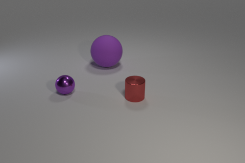
Figure 4: Visual Concept Repairing: NEMESYS achieves planning by performing differentiable meta-level reasoning. The left most image shows the start state, and the right most image shows the goal state. Taking these states as inputs, NEMESYS performs differentiable forward reasoning using meta-level clauses that simulate the planning steps and generate intermediate states (two images in the middle) and actions from start state to reach the goal state. (Best viewed in color)
### 4.3 Avoiding Infinite Loops
Differentiable forward chaining [17], unfortunately, can generate infinite computations. A pathological example:
| | $\displaystyle\mathtt{edge(a,b).\ edge(b,a).}\ \mathtt{edge(b,c).}\quad\mathtt{ path(A,A,[\ ]).}\quad$ | |
| --- | --- | --- |
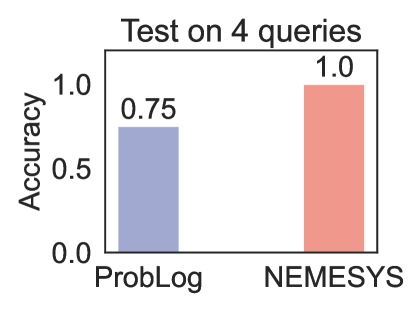
<details>
<summary>x4.png Details</summary>
### Visual Description
## Bar Chart: Test on 4 queries
### Overview
The image is a vertical bar chart comparing the accuracy of two systems, ProbLog and NEMESYS, on a test consisting of 4 queries. The chart clearly shows a performance difference between the two systems.
### Components/Axes
* **Chart Title:** "Test on 4 queries" (centered at the top).
* **Y-Axis:**
* **Label:** "Accuracy" (rotated vertically on the left side).
* **Scale:** Linear scale from 0.0 to 1.0.
* **Major Tick Marks:** 0.0, 0.5, 1.0.
* **X-Axis:**
* **Categories:** Two categories are labeled below their respective bars: "ProbLog" (left) and "NEMESYS" (right).
* **Data Series (Bars):**
* **ProbLog Bar:** A blue bar positioned on the left side of the chart. The numerical value `0.75` is displayed directly above it.
* **NEMESYS Bar:** A red/salmon-colored bar positioned on the right side of the chart. The numerical value `1.0` is displayed directly above it.
* **Legend:** Not present as a separate element. The categories are identified by the x-axis labels directly beneath each bar.
### Detailed Analysis
* **ProbLog:** The blue bar reaches a height corresponding to an accuracy value of **0.75** (or 75%).
* **NEMESYS:** The red bar reaches the maximum height of the y-axis, corresponding to an accuracy value of **1.0** (or 100%).
* **Visual Trend:** The NEMESYS bar is visibly taller than the ProbLog bar, indicating a higher accuracy score.
### Key Observations
1. **Perfect Score:** NEMESYS achieved a perfect accuracy score of 1.0 on the test.
2. **Performance Gap:** There is a significant 0.25 (25 percentage point) difference in accuracy between NEMESYS (1.0) and ProbLog (0.75).
3. **Test Scope:** The evaluation was conducted on a small set of 4 queries, as stated in the title.
### Interpretation
The data demonstrates that for this specific test set of 4 queries, the NEMESYS system performed flawlessly, while the ProbLog system made errors, achieving 75% accuracy. This suggests that NEMESYS may be more effective or better suited for the type of reasoning or problem-solving required by these particular queries. The chart serves as a direct, visual comparison highlighting NEMESYS's superior performance in this limited evaluation. The small number of queries (4) should be noted, as it may not be representative of performance on a larger, more diverse dataset.
</details>
Figure 5: Performance (accuracy; the higher, the better)on four queries. (Best viewed in color)
It defines a simple graph over three nodes $(a,b,c)$ with three edges, $(a-b,b-a,b-c)$ as well as paths in graphs in general. Specifically, $\mathtt{path}/3$ defines how to find a path between two nodes in a recursive way. The base case is $\mathtt{path(A,A,[])}$ , meaning that any node $\mathtt{A}$ is reachable from itself. The recursion then says, if there is an edge from node $\mathtt{A}$ to node $\mathtt{B}$ , and there is a path from node $\mathtt{B}$ to node $\mathtt{C}$ , then there is a path from node $\mathtt{A}$ to node $\mathtt{C}$ . Unfortunately, this generates an infinite loop $\mathtt{[edge(a,b),edge(b,a),edge(a,b),\ldots]}$ when computing the path from $a$ to $c$ , since this path can always be extended potentially also leading to the node $c$ .
Fortunately, NEMESYS allows one to avoid infinite loops by memorizing the proof-depth, i.e., we simply implement a limited proof-depth strategy on the meta-level:
| | $\displaystyle\mathtt{li((A,B),DPT)}\texttt{:-}\mathtt{li(A,DPT)},\mathtt{li(B, DPT).}$ | |
| --- | --- | --- |
With this proof strategy, NEMESYS gets the path $\mathtt{path(a,c,[edge(a,b),edge(b,c)])=true}$ in three steps. For simplicity, we omit the proof part in the atom. Using the second rule and the first rule recursively, the meta interpreter finds $\mathtt{clause(path(a,c),(edge(a,b),path(b,c)))}$ and $\mathtt{clause(path(b,c),(edge(b,c),path(c,c)))}$ . Finally, the meta interpreter finds a clause, whose head is $\mathtt{li(path(c,c),1)}$ and the body is true.
Since forward chaining gets stuck in the infinite loop, we choose ProbLog [47] as our baseline comparison. We test NEMESYS and ProbLog using four queries, including one query which calls the recursive rule. ProbLog fails to return the correct answer on the query which calls the recursive rule. The comparison is summarized in Fig. 5. We provide the four test queries in Appendix A.
### 4.4 Differentiable First-Order Logical Planning
As the fourth meta interpreter, we demonstrate NEMESYS as a differentiable planner. Consider Fig. 4 where NEMESYS was asked to put all objects of a start image onto a line. Each start and goal state is represented as a visual scene, which is generated in the CLEVR [18] environment. By adopting a perception model, e.g., YOLO [42] or slot attention [45], NEMESYS obtains logical representations of the start and end states:
| | $\displaystyle\mathtt{start}$ | $\displaystyle=\{\mathtt{pos(obj0,(1,3)),\ldots,pos(obj4,(2,1))}\},$ | |
| --- | --- | --- | --- |
where $\mathtt{pos/2}$ describes the $2$ -dim positions of objects. NEMESYS solves this planning task by performing differentiable reasoning using the meta-level program:
| | $\displaystyle\mathtt{plan(Start\_state,}\mathtt{New\_state,Goal\_state,[Action ,Old\_stack])}\textbf{:-}$ | |
| --- | --- | --- |
The first meta rule presents the recursive rule for plan generation, and the second rule gives the successful termination condition for the plan when the $\mathtt{Goal\_state}$ is reached, where $\mathtt{equal/2}$ checks whether the $\mathtt{Current\_state}$ is the $\mathtt{Goal\_state}$ and the $\mathtt{planf/3}$ contains $\mathtt{Start\_state}$ , $\mathtt{Goal\_state}$ and the needed action sequences $\mathtt{Move\_stack}$ from $\mathtt{Start\_state}$ to reach the $\mathtt{Goal\_state}$ .
The predicate $\mathtt{plan/4}$ takes four entries as inputs: $\mathtt{Start\_state}$ , $\mathtt{State}$ , $\mathtt{Goal\_state}$ and $\mathtt{Move\_stack}$ . The $\mathtt{move/3}$ predicate uses $\mathtt{Action}$ to push $\mathtt{Old\_state}$ to $\mathtt{New\_state}$ . $\mathtt{condition\_met/2}$ checks if the state’s preconditions are met. When the preconditions are met, $\mathtt{change\_state/2}$ changes the state, and $\mathtt{plan/4}$ continues the recursive search.
To reduce memory usage, we split the move action in horizontal and vertical in the experiment. For example, NEMESYS represents an action to move an object in the horizontal direction right by $\mathtt{1}$ step using meta-level atom:
| | $\displaystyle\mathtt{move(}$ | $\displaystyle\mathtt{move\_right},\mathtt{pos\_hori(Object,X),}\mathtt{pos\_ hori(Object,X}\texttt{+}\mathtt{1)).}$ | |
| --- | --- | --- | --- |
where $\mathtt{move\_right}$ represents the action, $\mathtt{X+1}$ represents arithmetic sums over (positive) integers, encoded as $\mathtt{0,succ(0),succ(succ(0))}$ and so on as terms. Performing reasoning on the meta-level clause with $\mathtt{plan}$ simulates a step as a planner, i.e., it computes preconditions, and applies actions to compute states after taking the actions. Fig. 4 summarizes one of the experiments performed using NEMESYS on the Visual Concept Repairing task. We provided the start and goal states as visual scenes containing varying numbers of objects with different attributes. The left most image of Fig. 4 shows the start state, and the right most image shows the goal state, respectively. NEMESYS successfully moved objects to form a line. For example, to move $\mathtt{obj0}$ from $\mathtt{(1,1)}$ to $\mathtt{(3,1)}$ , NEMESYS deduces:
| | $\displaystyle\mathtt{planf(}$ | $\displaystyle\mathtt{pos\_hori(obj0,1)},\mathtt{pos\_hori(obj0,3),}\mathtt{[ move\_right,move\_right]).}$ | |
| --- | --- | --- | --- |
This shows that NEMESYS is able to perceive objects from an image, reason about the image, and edit the image through planning. To the best of our knowledge, this is the first differentiable neuro-symbolic system equipped with all of these abilities. We provide more Visual Concept Repairing tasks in Appendix B.
### 4.5 Differentiable Causal Reasoning
As the last meta interpreter, we show that NEMESYS exhibits superior performance compared to the existing forward reasoning system by having the causal reasoning ability. Notably, given a causal Bayesian network, NEMESYS can perform the $\mathtt{do}$ operation (deleting the incoming edges of a node) [28] on arbitrary nodes and perform causal reasoning without the necessity of re-executing the entire system, which is made possible through meta-level programming.
<details>
<summary>x5.png Details</summary>
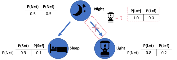
### Visual Description
## Diagram: Bayesian Network with Conditional Probability Tables
### Overview
The image displays a probabilistic graphical model, specifically a Bayesian network, illustrating the relationships between three binary variables: **Night (N)**, **Sleep (S)**, and **Light (L)**. The diagram includes nodes, directed edges representing dependencies, and associated conditional probability tables (CPTs). An observation is indicated for the "Light" variable.
### Components/Axes
1. **Nodes (Variables):**
* **Night (N):** Top-center node. Icon: Crescent moon and stars.
* **Sleep (S):** Bottom-left node. Icon: Person in bed.
* **Light (L):** Bottom-right node. Icon: Table lamp.
2. **Edges (Dependencies):**
* A **solid blue arrow** points from **Night** to **Sleep**, indicating a direct probabilistic dependence.
* A **dashed blue arrow** with a **red cross (X)** over it points from **Night** to **Light**. This typically signifies a direct dependency that is being considered, blocked, or is the subject of analysis (e.g., in the context of d-separation or when evidence is observed).
3. **Observation Notation:**
* To the right of the **Night** node, an hourglass icon is shown with the text **`= t`**. This symbolizes that the variable **Light (L)** is **observed to be true (t)**. This observation is linked to the Light node via the dashed arrow.
4. **Probability Tables:**
* **Prior for Night:** Located top-left.
* `P(N=t) = 0.5`
* `P(N=f) = 0.5`
* **Conditional Probability for Sleep (given N=t):** Located bottom-left, next to the Sleep node.
* `P(S=t | N=t) = 0.9`
* `P(S=f | N=t) = 0.1`
* **Conditional Probability for Light (given N=t):** Located bottom-right, next to the Light node.
* `P(L=t | N=t) = 0.8`
* `P(L=f | N=t) = 0.2`
* **Probability for Light (Observed):** Located top-right, enclosed in a **red dashed border**.
* `P(L=t) = 1.0`
* `P(L=f) = 0.0`
* This table represents the state of knowledge after observing that `L = t`.
### Detailed Analysis
* **Network Structure:** The core structure is `N -> S` and `N -> L`. The dashed, crossed arrow from N to L, combined with the observation `L=t`, suggests the diagram is illustrating a scenario where the direct link between Night and Light is being evaluated in the presence of evidence.
* **Probability Values:**
* The prior probability of Night being true is uniform (0.5).
* If it is Night (`N=t`), there is a high probability (0.9) of Sleep (`S=t`).
* If it is Night (`N=t`), there is a moderately high probability (0.8) of the Light being on (`L=t`).
* The observation `L=t` is treated as a certainty (`P(L=t)=1.0`), which would be used to update beliefs about other variables in the network (e.g., calculating `P(N=t | L=t)`).
### Key Observations
1. **Evidence Instantiation:** The key feature is the **observed state of Light (`L=t`)**, highlighted by the red-dashed table and the `= t` notation. This turns the Light node into an evidence variable.
2. **Blocked Path Symbolism:** The red cross over the dashed arrow from Night to Light is a critical visual cue. In the context of the observed evidence `L=t`, this likely represents that the direct causal path from N to L is **"blocked" or "explained away"** when we condition on the effect (L). This is a common concept in Bayesian networks for explaining phenomena like the "explaining away" effect or in d-separation.
3. **Layout:** The legend/tables are spatially grounded next to their corresponding nodes. The observation notation is placed between the Night and Light nodes, visually associating the evidence with the Light variable.
### Interpretation
This diagram is a pedagogical tool for explaining **probabilistic inference in Bayesian networks**, specifically focusing on the impact of **observed evidence**.
* **What it Demonstrates:** It shows how observing an effect (Light is on, `L=t`) changes the probabilistic landscape. The crossed arrow suggests that once we know `L=t`, the direct influence of Night on Light is no longer relevant for inference; instead, we use the evidence to reason *backwards* about the cause (Night). For example, one would compute the posterior probability `P(N=t | L=t)` using Bayes' rule, which would be higher than the prior `P(N=t)=0.5` because `P(L=t | N=t)=0.8` is high.
* **Relationships:** The solid arrow `N->S` remains active. The state of Night still directly influences Sleep. The diagram sets up a scenario to explore how evidence on one branch (Light) might affect beliefs about a common cause (Night) and, by extension, other effects (Sleep) that are not directly connected to the evidence.
* **Notable Anomaly/Concept:** The primary "anomaly" is the **crossed-out arrow**. This is not a data anomaly but a conceptual notation. It visually encodes a key principle: in a Bayesian network, when you condition on a node (observe it), it can block the flow of information between its ancestors and other descendants. The diagram is likely part of a lesson on **d-separation** or **explaining away**, where observing `L=t` makes `N` and other causes of `L` (if there were any) dependent in a way that "explains" the observation.
</details>
Figure 6: Performing differentiable causal reasoning and learning using NEMESYS. Given a causal Bayesian network, NEMESYS can easily perform the do operation (delete incoming edges) on arbitrary nodes and capture the causal effects on different nodes (for example, the probability of the node $\mathtt{Light}$ after intervening) without rerunning the entire system. Furthermore, NEMESYS is able to learn the unobserved $\mathtt{do}$ operation with its corresponding value using gradient descent based on the given causal graph and observed data. (Best viewed in color)
The $\mathtt{do}$ operator, denoted as $\mathtt{do(X)}$ , is used to represent an intervention on a particular variable $\mathtt{X}$ in a causal learning system, regardless of the actual value of the variable. For example, Fig. 6 shows a causal Bayesian network with three nodes and the probability distribution of the nodes before and after the $\mathtt{do}$ operation. To investigate how the node $\mathtt{Light}$ affects the rest of the system, we firstly cut the causal relationship between the node $\mathtt{Light}$ and all its parent nodes, then we assign a new value to the node and we investigate the probability of other nodes. To enable NEMESYS to perform a $\mathtt{do}$ operation on the node $\mathtt{Light}$ , we begin by representing the provided causal Bayesian network in Fig. 6 using:
| | $\displaystyle\mathtt{0.5}\texttt{:}\ \mathtt{Night}.\quad\mathtt{0.9}\texttt{: }\ \mathtt{Sleep}\texttt{:-}\mathtt{Night}.\quad\mathtt{0.8}\texttt{:}\ \mathtt{Light}\texttt{:-}\mathtt{Night}.$ | |
| --- | --- | --- |
where the number of an atom indicates the probability of the atom being true, and the number of a clause indicates the conditional probability of the head being true given the body being true.
We reuse the meta predicate $\mathtt{assert\_probs/1/[atom]}$ and introduce three new meta predicates: $\mathtt{prob/1/[atom]}$ , $\mathtt{probs/1/[atoms]}$ and $\mathtt{probs\_do/1/[atoms,atom]}$ . Since we cannot deal with the uncountable, infinite real numbers within our logic, we make use of the weight associated with ground meta atoms to represent the probability of the atom. For example, we use the weight of the meta atom $\mathtt{prob(Atom)}$ to represent the probability of the atom $\mathtt{Atom}$ . We use the weight of the meta atom $\mathtt{probs(Atoms)}$ to represent the joint probability of a list of atoms $\mathtt{Atoms}$ , and the weight of $\mathtt{probs\_do(AtomA,AtomB)}$ to represent the probability of the atom $\mathtt{AtomA}$ after performing the do operation $\mathtt{do(AtomB)}$ . We modify the meta interpreter as:
| | $\displaystyle\mathtt{prob(Head)}\texttt{:-}\mathtt{assert\_probs((Head\texttt{ :-}Body))},\mathtt{probs(Body).}$ | |
| --- | --- | --- |
where the first three rules calculate the probability of a node before the intervention, the joint probability is approximated using the first and second rule by iteratively multiplying each atom. The fourth rule assigns the probability of the atom $\mathtt{Atom}$ using the $\mathtt{do}$ operation. The fifth to the eighth calculate the probability after the $\mathtt{do}$ intervention by looping over each atom and multiplying them.
For example, after performing $\mathtt{do(Light)}$ and setting the probability of $\mathtt{Light}$ as $1.0$ . NEMESYS returns the weight of $\mathtt{probs\_do(Light,Light)}$ as the probability of the node $\mathtt{Light}$ (Fig. 6 red box) after the intervention $\mathtt{do(Light)}$ .
### 4.6 Gradient-based Learning in NEMESYS
NEMESYS alleviates the limitations of frameworks such as DeepProbLog [21] by having the ability of not only performing differentiable parameter learning but also supporting differentiable structure learning (in our experiment, NEMESYS learns the weights of the meta rules while adapting to solve different tasks). We now introduce the learning ability of NEMESYS.
#### 4.6.1 Parameter Learning
Consider a scenario in which a patient can only experience effective treatment when two types of medicine synergize, with the effectiveness contingent on the dosage of each drug. Suppose we have known the dosages of two medicines and the causal impact of the medicines on the patient, however, the observed effectiveness does not align with expectations. It is certain that some interventions have occurred in the medicine-patient causal structure (such as an incorrect dosage of one medicine, which will be treated as an intervention using the $\mathtt{do}$ operation). However, the specific node (patient or the medicines) on which the $\mathtt{do}$ operation is executed, and the values assigned to the $\mathtt{do}$ operator remain unknown. Conducting additional experiments on patients by altering medicine dosages to uncover the $\mathtt{do}$ operation is both unethical and dangerous.
With NEMESYS at hand, we can easily learn the unobserved $\mathtt{do}$ operation with its assigned value. We abstract the problem using a three-node causal Bayesian network:
$$
\mathtt{1.0:medicine\_a.}\quad\mathtt{1.0:medicine\_b.}\quad\mathtt{0.9:
patient}\texttt{:-}\mathtt{medicine\_a,medicine\_b.}
$$
where the number of the atoms indicates the dosage of each medicine, and the number of the clause indicates the conditional probability of the effectiveness of the patient given these two medicines. Suppose there is only one unobserved $\mathtt{do}$ operation.
To learn the unknown $\mathtt{do}$ operation, we define the loss as the Binary Cross Entropy (BCE) loss between the observed probability $\mathbf{p}_{target}$ and the predicted probability of the target atom $\mathbf{p}_{predicted}$ . The predicted probability $\mathbf{p}_{predicted}$ is computed as: $\mathbf{p}_{predicted}=\mathbf{v}^{(T)}\left[I_{\mathcal{G}}(\operatorname{ target\_atom})\right]$ , where $I_{\mathcal{G}}(x)$ is a function that returns the index of target atom in $\mathcal{G}$ , $\mathbf{v}[i]$ is the $i$ -th element of $\mathbf{v}$ . $\mathbf{v}^{(T)}$ is the valuation tensor computed by $T$ -step forward reasoning based on the initial valuation tensor $\mathbf{v}^{(0)}$ , which is composed of the initial valuation of $\mathtt{do}$ and other meta ground atoms. Since the valuation of $\mathtt{do}$ atom is the only changing parameter, we set the gradient of other parameters as $0 0$ . We minimize the loss w.r.t. $\mathtt{do(X)}$ : $\underset{\mathtt{do(X)}}{\mathtt{minimize}}\quad\mathtt{L_{loss}}=\mathtt{BCE }(\mathbf{p}_{target},\mathbf{p}_{predicted}\mathtt{(do(X)))}.$ Fig. 7 summarizes the loss curve of the three $\mathtt{do}$ operators during learning using one target (Fig. 7 left) and three targets (Fig. 7 right). For the three targets experiment, $\mathbf{p}_{target}$ consists of three observed probabilities (the effectiveness of the patient and the dosages of two medicines), for the experiment with one target, $\mathbf{p}_{target}$ only consists of the observed the effectiveness of the patient.
We randomly initialize the probability of the three $\mathtt{do}$ operators and choose the one, which achieves the lowest loss as the right $\mathtt{do}$ operator. In the three targets experiment, the blue curve achieves the lowest loss, with its corresponding value converges to the ground truth value, while in the one target experiment, three $\mathtt{do}$ operators achieve equivalent performance. We provide the value curves of three $\mathtt{do}$ operators and the ground truth $\mathtt{do}$ operator with its value in Appendix C.
<details>
<summary>x6.png Details</summary>
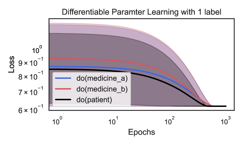
### Visual Description
## Line Chart: Differentiable Parameter Learning with 1 label
### Overview
This is a log-log line chart illustrating the reduction in model loss over training epochs for three distinct intervention groups, each with a shaded band representing uncertainty/confidence intervals. The chart tracks learning performance across a logarithmic scale of epochs, showing convergence of all groups to a similar final loss value.
### Components/Axes
- **Title**: "Differentiable Parameter Learning with 1 label" (centered at the top of the chart)
- **Y-axis**: Labeled "Loss", using a logarithmic scale. Axis markers (bottom to top): `6×10⁻¹`, `7×10⁻¹`, `8×10⁻¹`, `9×10⁻¹`, `10⁰`
- **X-axis**: Labeled "Epochs", using a logarithmic scale. Axis markers (left to right): `10⁰`, `10¹`, `10²`, `10³`
- **Legend (bottom-left, overlapping the chart area)**:
- Blue line: `do(medicine_a)`
- Red line: `do(medicine_b)`
- Black line: `do(patient)`
- **Shaded Uncertainty Bands**: Each line has a corresponding shaded region (light purple for `do(medicine_a)`, darker purple for `do(medicine_b)`, dark gray for `do(patient)`) indicating variability/confidence in the loss measurement.
### Detailed Analysis
1. **Trend Verification**:
- All three lines exhibit a consistent downward trend as epochs increase, meaning loss decreases with more training iterations, with the steepest drop occurring between `10²` and `10³` epochs.
- `do(patient)` (black line): Starts at ~8.5×10⁻¹ at `10⁰` epochs, decreases gradually, then steeply after `10²` epochs, converging to ~6×10⁻¹ at `10³` epochs. Its shaded band is the narrowest, indicating the lowest uncertainty.
- `do(medicine_a)` (blue line): Starts at ~8.8×10⁻¹ at `10⁰` epochs, follows a parallel downward curve to the patient group, converging to ~6×10⁻¹ at `10³` epochs. Its shaded band is wider than the patient group's, but narrower than the medicine_b group's.
- `do(medicine_b)` (red line): Starts at ~9.2×10⁻¹ at `10⁰` epochs (the highest initial loss), decreases in a similar curve, converging to ~6×10⁻¹ at `10³` epochs. Its shaded band is the widest, indicating the highest uncertainty.
### Key Observations
- All three intervention groups converge to the same final loss value (~6×10⁻¹) at `10³` epochs.
- Initial loss is highest for `do(medicine_b)`, followed by `do(medicine_a)`, then `do(patient)`.
- Uncertainty (shaded band width) is highest for `do(medicine_b)` and lowest for `do(patient)`.
- The rate of loss reduction is consistent across all groups, with the most rapid improvement occurring in the later training stages (100 to 1000 epochs).
### Interpretation
This chart demonstrates that differentiable parameter learning with a single label enables loss reduction across all three intervention groups, with full convergence to equivalent performance after sufficient training. The `do(patient)` group shows the most stable, predictable learning trajectory (lowest initial loss and uncertainty), suggesting this intervention is the most efficient in early training stages. `do(medicine_b)` has the highest initial loss and variability, indicating more unpredictable early learning, but still reaches the same final performance as the other groups. This implies that while initial performance and stability vary, all interventions can achieve identical loss levels with enough training epochs, meaning the model can adapt to all three interventions given sufficient training time.
</details>
<details>
<summary>x7.png Details</summary>
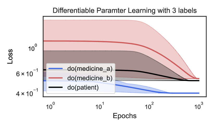
### Visual Description
## Line Chart: Differentiable Parameter Learning with 3 labels
### Overview
The image is a line chart titled "Differentiable Paramter Learning with 3 labels" (note: "Parameter" is misspelled as "Paramter" in the title). It displays the training loss over epochs for three different causal interventions, labeled using the `do()`-operator notation from causal inference. The chart uses a logarithmic scale on both the x-axis (Epochs) and y-axis (Loss). Each line is accompanied by a shaded region representing the confidence interval or variance around the mean loss.
### Components/Axes
* **Title:** "Differentiable Paramter Learning with 3 labels"
* **X-Axis:**
* **Label:** "Epochs"
* **Scale:** Logarithmic (base 10).
* **Major Ticks/Markers:** `10^0` (1), `10^1` (10), `10^2` (100), `10^3` (1000).
* **Y-Axis:**
* **Label:** "Loss"
* **Scale:** Logarithmic (base 10).
* **Major Ticks/Markers:** `4 x 10^-1` (0.4), `6 x 10^-1` (0.6), `10^0` (1.0).
* **Legend:** Located in the bottom-left quadrant of the chart area.
* **Blue Line:** `do(medicine_a)`
* **Red Line:** `do(medicine_b)`
* **Black Line:** `do(patient)`
### Detailed Analysis
**Trend Verification & Data Point Extraction (Approximate Values):**
1. **Series: `do(medicine_a)` (Blue Line)**
* **Trend:** The line shows a steady, monotonic decrease from the start, flattening out significantly after approximately 100 epochs.
* **Data Points:**
* Epoch 1 (`10^0`): Loss ≈ 0.52
* Epoch 10 (`10^1`): Loss ≈ 0.48
* Epoch 100 (`10^2`): Loss ≈ 0.41
* Epoch 1000 (`10^3`): Loss ≈ 0.40 (plateaued)
* **Confidence Interval (Blue Shading):** Relatively narrow throughout, suggesting low variance in the loss for this intervention.
2. **Series: `do(medicine_b)` (Red Line)**
* **Trend:** The line starts at the highest loss value, remains nearly flat for the first ~10 epochs, then begins a steep, consistent decline. It converges toward the other lines but remains the highest at the final epoch.
* **Data Points:**
* Epoch 1 (`10^0`): Loss ≈ 1.2
* Epoch 10 (`10^1`): Loss ≈ 1.15
* Epoch 100 (`10^2`): Loss ≈ 0.70
* Epoch 1000 (`10^3`): Loss ≈ 0.50
* **Confidence Interval (Red Shading):** Very wide initially (spanning from ~0.6 to ~2.0 at epoch 1), indicating high initial uncertainty or variance. The interval narrows considerably as training progresses.
3. **Series: `do(patient)` (Black Line)**
* **Trend:** The line shows a gradual, consistent decrease from an intermediate starting point. Its slope is less steep than the red line's descent but more pronounced than the blue line's initial slope.
* **Data Points:**
* Epoch 1 (`10^0`): Loss ≈ 0.62
* Epoch 10 (`10^1`): Loss ≈ 0.60
* Epoch 100 (`10^2`): Loss ≈ 0.55
* Epoch 1000 (`10^3`): Loss ≈ 0.48
* **Confidence Interval (Grey/Black Shading):** Moderate width, consistently positioned between the blue and red intervals.
### Key Observations
* **Final Performance Hierarchy:** At 1000 epochs, the final loss values are ordered: `do(medicine_a)` (lowest, ~0.40) < `do(patient)` (~0.48) < `do(medicine_b)` (highest, ~0.50).
* **Convergence Behavior:** All three loss curves are converging, but at different rates and from different starting points. The red line (`do(medicine_b)`) shows the most dramatic improvement.
* **Uncertainty Dynamics:** The uncertainty (shaded area) for `do(medicine_b)` is exceptionally high at the start of training but diminishes significantly, suggesting the model becomes more confident in its parameter estimates for this intervention over time. The other two interventions show more stable uncertainty.
* **Scale:** The use of log-log axes emphasizes the early-stage learning dynamics and allows for clear visualization of the wide range of loss values, especially for the red line.
### Interpretation
This chart visualizes the learning process of a differentiable model tasked with estimating parameters for three distinct causal interventions. The `do()`-operator notation implies the model is learning the effect of forcing a variable (medicine_a, medicine_b, or patient state) to a specific value.
* **What the data suggests:** The intervention `do(medicine_a)` appears to be the "easiest" for the model to learn, starting with a lower loss and converging quickly to the best final performance with low uncertainty. In contrast, `do(medicine_b)` is initially very challenging (high loss and high variance) but benefits the most from prolonged training. The `do(patient)` intervention represents a middle ground in terms of learning difficulty and final performance.
* **Relationship between elements:** The chart directly compares the learnability and final model fit for different causal questions. The converging trends suggest that with sufficient training (epochs), the model can reduce the error for all interventions, though inherent differences in complexity or data availability may lead to different final loss levels.
* **Notable Anomalies/Patterns:** The most striking pattern is the dramatic shift in the red line (`do(medicine_b)`). Its high initial loss and variance could indicate that the causal effect of `medicine_b` is more complex, noisier, or less supported by the initial data than the effects of `medicine_a` or the baseline `patient` state. The eventual convergence, however, shows the differentiable learning framework is effective at overcoming this initial difficulty. The chart essentially tells a story of varying learning trajectories for different causal parameters within the same model.
</details>
Figure 7: NEMESYS performs differentiable parameter learning using gradient descent. Based on the given data (one or three targets), NEMESYS is asked to learn the correct $\mathtt{do}$ operator and its corresponding value (which we didn’t show in the images). The loss curve is averaged on three runs. The shadow area indicates the min and max number of the three runs. (Best viewed in color)
<details>
<summary>x8.png Details</summary>
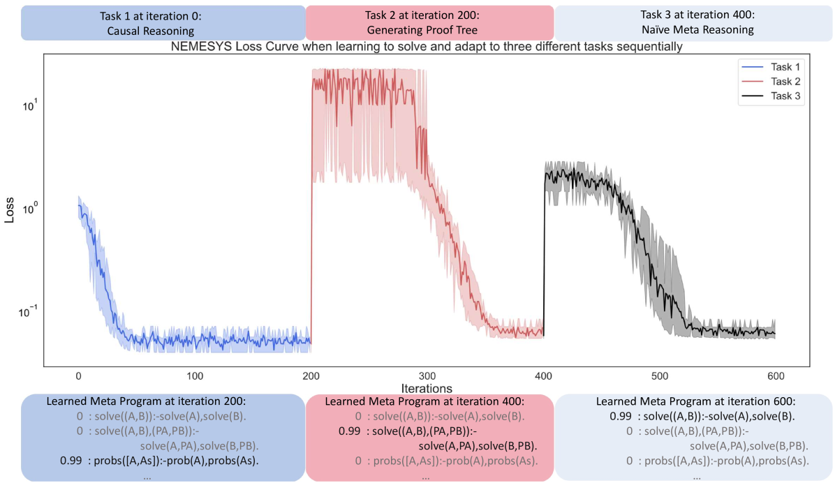
### Visual Description
## [Line Chart]: NEMESYS Loss Curve for Sequential Task Learning
### Overview
The image is a line chart titled *"NEMESYS Loss Curve when learning to solve and adapt to three different tasks sequentially"*. It visualizes the loss (y-axis, logarithmic scale) over iterations (x-axis, 0–600) for three tasks: **Task 1 (Causal Reasoning)**, **Task 2 (Generating Proof Tree)**, and **Task 3 (Naive Meta Reasoning)**. Below the chart, three text boxes display "Learned Meta Program" at iterations 200, 400, and 600.
### Components/Axes
- **Title**: *"NEMESYS Loss Curve when learning to solve and adapt to three different tasks sequentially"*
- **X-axis**: *"Iterations"* (markers: 0, 100, 200, 300, 400, 500, 600).
- **Y-axis**: *"Loss"* (logarithmic scale: \(10^{-1}\), \(10^0\), \(10^1\)).
- **Legend** (top-right):
- Blue line: *Task 1 (Causal Reasoning)*
- Red line: *Task 2 (Generating Proof Tree)*
- Black line: *Task 3 (Naive Meta Reasoning)*
- **Task Labels** (top, color-coded):
- Left (blue): *"Task 1 at iteration 0: Causal Reasoning"*
- Middle (red): *"Task 2 at iteration 200: Generating Proof Tree"*
- Right (black): *"Task 3 at iteration 400: Naive Meta Reasoning"*
- **Text Boxes** (bottom, color-coded):
- Left (blue): *"Learned Meta Program at iteration 200:"* (3 lines of code-like text).
- Middle (red): *"Learned Meta Program at iteration 400:"* (3 lines).
- Right (black): *"Learned Meta Program at iteration 600:"* (3 lines).
### Detailed Analysis (Chart)
#### Task 1 (Blue Line)
- **Trend**: Starts at iteration 0 with loss ~\(10^0\) (1.0), decreases rapidly, and stabilizes at ~\(10^{-1}\) (0.1) by iteration 100. Remains flat until iteration 200.
#### Task 2 (Red Line)
- **Trend**: Starts at iteration 200 with loss ~\(10^1\) (10), decreases rapidly, and stabilizes at ~\(10^{-1}\) (0.1) by iteration 300. Remains flat until iteration 400.
#### Task 3 (Black Line)
- **Trend**: Starts at iteration 400 with loss ~\(10^0\) (1.0), decreases rapidly, and stabilizes at ~\(10^{-1}\) (0.1) by iteration 500. Remains flat until iteration 600.
### Content Details (Text Boxes)
#### Learned Meta Program at iteration 200 (Blue Box)
- Line 1: `0 : solve((A,B)):-solve(A),solve(B).`
- Line 2: `0 : solve((A,B),(PA,PB)):- solve(A,PA),solve(B,PB).`
- Line 3: `0.99 : probs([A,As]) :-prob(A),probs(As).`
#### Learned Meta Program at iteration 400 (Red Box)
- Line 1: `0 : solve((A,B)):-solve(A),solve(B).`
- Line 2: `0.99 : solve((A,B),(PA,PB)):- solve(A,PA),solve(B,PB).`
- Line 3: `0 : probs([A,As]) :-prob(A),probs(As).`
#### Learned Meta Program at iteration 600 (Black Box)
- Line 1: `0.99 : solve((A,B)):-solve(A),solve(B).`
- Line 2: `0 : solve((A,B),(PA,PB)):- solve(A,PA),solve(B,PB).`
- Line 3: `0 : probs([A,As]) :-prob(A),probs(As).`
### Key Observations
1. **Loss Stabilization**: All three tasks stabilize at a low loss (~\(10^{-1}\)) after ~100 iterations of introduction, indicating consistent performance across tasks.
2. **Meta Program Adaptation**: The "Learned Meta Program" shifts the high-probability (0.99) rule to match the current task:
- Iteration 200: `probs([A,As])` rule (Task 1).
- Iteration 400: `solve((A,B),(PA,PB))` rule (Task 2).
- Iteration 600: `solve((A,B))` rule (Task 3).
3. **Task Complexity**: Task 2 (Generating Proof Tree) starts with a higher loss (\(10^1\)) than Tasks 1 and 3 (\(10^0\)), suggesting greater initial complexity, but still stabilizes quickly.
### Interpretation
- **Sequential Learning**: The chart demonstrates the model’s ability to learn and adapt to three distinct tasks sequentially. Each new task (introduced at 0, 200, 400) starts with a higher loss but rapidly stabilizes, showing effective transfer learning or meta-learning.
- **Meta-Program Evolution**: The "Learned Meta Program" text boxes reveal how the model’s internal reasoning rules (meta-programs) evolve to prioritize the current task’s requirements. This suggests the model dynamically adjusts its strategy to solve each task.
- **Consistent Performance**: All tasks stabilize at a similar low loss, indicating the model achieves robust performance across diverse tasks after adaptation.
- **Task Introduction Timing**: Tasks are introduced at regular intervals (0, 200, 400), allowing the model to build on prior learning, which may explain the rapid stabilization of new tasks.
This analysis captures all textual, graphical, and interpretive details, enabling reconstruction of the image’s content without visual reference.
</details>
Figure 8: NEMESYS can learn to solve and adapt itself to different tasks during learning using gradient descent. In this experiment, we train NEMESYS to solve three different tasks: causal reasoning, generating proof trees and naive meta reasoning sequentially (each task is represented by a unique color encoding). The loss curve is averaged on five runs, with the shadow area indicating the minimum and maximum number of the five runs. For readability, the learned complete meta program is not shown in the image. (Best viewed in color)
#### 4.6.2 Structure Learning
Besides parameter learning, NEMESYS can also perform differentiable structure learning (we provide the candidate meta rules and learn the weights of these meta rules using gradient descent). In this experiment, different tasks are presented at distinct time steps throughout the learning process. NEMESYS is tasked with acquiring the ability to solve and adapt to these diverse tasks.
Following Sec. 3.2, we make use of the meta rule weight matrix $\mathbf{W}=[{\bf w}_{1},\ldots,{\bf w}_{M}]$ to select the rules. We take the softmax of each weight vector ${\bf w}_{j}\in\mathbf{W}$ to choose $M$ meta rules out of $C$ meta rules. To adapt to different tasks, the weight matrix $\mathbf{W}$ is learned based on the loss, which is defined as the BCE loss between the probability of the target $\mathbf{p}_{target}$ and the predicted probability $\mathbf{p}_{predicted}$ , where $\mathbf{p}_{predicted}$ is the probability of the target atoms calculated using the learned program. $\mathbf{p}_{predicted}$ is computed as: $\mathbf{p}_{predicted}=\mathbf{v}^{(T)}\left[I_{\mathcal{G}}(\operatorname{ target\_atoms})\right]$ , where $I_{\mathcal{G}}(x)$ is a function that returns the indexes of target atoms in $\mathcal{G}$ , $\mathbf{v}[i]$ is the $i$ -th element of $\mathbf{v}$ and $\mathbf{v}^{(T)}$ is the valuation tensor computed by $T$ -step forward reasoning. We minimize the loss w.r.t. the weight matrix $\mathbf{W}$ : $\underset{\mathbf{W}}{\mathtt{minimize}}\quad\mathtt{L_{loss}}=\mathtt{BCE}( \mathbf{p}_{target},\mathbf{p}_{predicted}(\mathbf{W})).$
We randomly initialize the weight matrix $\mathbf{W}$ , and update the weights using gradient descent. We set the target $\mathbf{p}_{target}$ using positive target atoms and negative target atoms. For example, suppose we have the naive meta reasoning and generating proof tree as two tasks. To learn a program to generate the proof tree, we use the proof tree meta rules to generate positive examples, and use the naive meta rules to generate the negative examples.
We ask NEMESYS to solve three different tasks sequentially, which is initially, calculating probabilities using the first three rules of causal reasoning, then executing naive meta-reasoning. Finally, generating a proof tree. We set the program size to three and randomly initialize the weight matrix. Fig. 8 shows the learning process of NEMESYS which can automatically adapt to solve these three different tasks. We provide the accuracy curve and the candidate rules with the learned weights in Appendix D. We also compare NEMESYS with the baseline method DeepProbLog [21] (cf. Table. 4). Due to the limitations of DeepProbLog in adapting (meta) rule weights during learning, we initialize DeepProbLog with three variants as our baseline comparisons. The first variant involves fixed task 1 meta rule weights ( $\mathtt{1.0}$ ), with task 2 and task 3 meta rule weights being randomly initialized. In the second variant, task 2 meta rule weights are fixed ( $\mathtt{1.0}$ ), while task 1 and task 3 meta rule weights are randomly initialized, and this pattern continues for the subsequent variant. We provide NEMESYS with the same candidate meta rules, however, with randomly initialize weights. We compute the accuracy at iteration $\mathtt{200}$ , $\mathtt{400}$ and $\mathtt{600}$ .
### 4.7 Discussion
While NEMESYS achieves impressive results, it is worth considering some of the limitations of this work. In our current experiments for structure learning, candidates of meta-rules are provided. It is promising to integrate rule-learning techniques, e.g., mode declarations, meta-interpretive learning, and a more sophisticated rule search, to learn from less prior. Another limitation lies in the calculation, since our system is not able to handle real number calculation, we make use of the weight associated with the atom to approximate the value and do the calculation.
| | Test Task1 | Test Task2 | Test Task3 |
| --- | --- | --- | --- |
| DeepProbLog (T1) | 100 $\bullet$ | 14.29 | 0 |
| DeepProbLog (T2) | 0 | 100 $\bullet$ | 11.43 |
| DeepProbLog (T3) | 68.57 | 5.71 | 100 $\bullet$ |
| NEMESYS (ours) | 100 $\bullet$ | 100 $\bullet$ | 100 $\bullet$ |
Table 4: Performance (Accuracy; the higher, the better) on test split of three tasks. We compare NEMESYS with baseline method DeepProbLog [21] (with three variants). The accuracy is averaged on five runs. The best-performing models are denoted using $\bullet$ .
## 5 Conclusions
We proposed the framework of neuro-metasymbolic reasoning and learning. We realized a differentiable meta interpreter using the differentiable implementation of first-order logic with meta predicates. This meta-interpreter, called NEMESYS, achieves various important functions on differentiable logic programming languages using meta-level programming. We illustrated this on different tasks of visual reasoning, reasoning with explanations, reasoning with infinite loops, planning on visual scenes, performing the $\mathtt{do}$ operation within a causal Bayesian network and showed NEMESYS’s gradient-based capability of parameter learning and structure learning.
NEMESYS provides several interesting avenues for future work. One major limitation of NEMESYS is its scalability for large-scale meta programs. So far, we have mainly focused on specifying the syntax and semantics of new (domain-specific) differentiable logic programming languages, helping to ensure that the languages have some desired properties. In the future, one should also explore providing properties about programs written in a particular differentiable logic programming language and injecting the properties into deep neural networks via algorithmic supervision [50], as well as program synthesis. Most importantly, since meta programs in NEMESYS are parameterized, and the reasoning mechanism is differentiable, one can realize differentiable meta-learning easily, i.e., the reasoning system that learns how to perform reasoning better from experiences.
Acknowledgements. This work was supported by the Hessian Ministry of Higher Education, Research, Science and the Arts (HMWK) cluster project “The Third Wave of AI”. The work has also benefited from the Hessian Ministry of Higher Education, Research, Science and the Arts (HMWK) cluster project “The Adaptive Mind” and the Federal Ministry for Economic Affairs and Climate Action (BMWK) AI lighthouse project “SPAICER” (01MK20015E), the EU ICT-48 Network of AI Research Excellence Center “TAILOR” (EU Horizon 2020, GA No 952215), and the Collaboration Lab “AI in Construction” (AICO) with Nexplore/HochTief.
## References
Ramesh et al. [2022] Ramesh, A., Dhariwal, P., Nichol, A., Chu, C., Chen, M.: Hierarchical text-conditional image generation with clip latents. arXiv Preprint:2204.0612 (2022)
Stiennon et al. [2020] Stiennon, N., Ouyang, L., Wu, J., Ziegler, D., Lowe, R., Voss, C., Radford, A., Amodei, D., Christiano, P.F.: Learning to summarize with human feedback. Advances in Neural Information Processing Systems (NeurIPS) (2020)
Floridi and Chiriatti [2020] Floridi, L., Chiriatti, M.: Gpt-3: Its nature, scope, limits, and consequences. Minds and Machines 30, 681–694 (2020)
Reed et al. [2022] Reed, S., Zolna, K., Parisotto, E., Colmenarejo, S.G., Novikov, A., Barth-maron, G., Giménez, M., Sulsky, Y., Kay, J., Springenberg, J.T., et al.: A generalist agent. Transactions on Machine Learning Research (TMLR) (2022)
Ackerman and Thompson [2017] Ackerman, R., Thompson, V.A.: Meta-reasoning: Monitoring and control of thinking and reasoning. Trends in cognitive sciences 21 (8), 607–617 (2017)
Costantini [2002] Costantini, S.: Meta-reasoning: A survey. In: Computational Logic: Logic Programming and Beyond (2002)
Griffiths et al. [2019] Griffiths, T.L., Callaway, F., Chang, M.B., Grant, E., Krueger, P.M., Lieder, F.: Doing more with less: Meta-reasoning and meta-learning in humans and machines. Current Opinion in Behavioral Sciences 29, 24–30 (2019)
Russell and Wefald [1991] Russell, S., Wefald, E.: Principles of metareasoning. Artificial intelligence 49 (1-3), 361–395 (1991)
Schmidhuber [1987] Schmidhuber, J.: Evolutionary principles in self-referential learning, or on learning how to learn: the meta-meta-… hook. PhD thesis, Technische Universität München (1987)
Thrun and Pratt [1998] Thrun, S., Pratt, L.: Learning to Learn: Introduction and Overview, pp. 3–17. Springer, Boston, MA (1998)
Finn et al. [2017] Finn, C., Abbeel, P., Levine, S.: Model-agnostic meta-learning for fast adaptation of deep networks. In: Proceedings of the 34th International Conference on Machine Learning (ICML) (2017)
Hospedales et al. [2022] Hospedales, T.M., Antoniou, A., Micaelli, P., Storkey, A.J.: Meta-learning in neural networks: A survey. IEEE Trans. Pattern Anal. Mach. Intell. 44 (9), 5149–5169 (2022)
Kim et al. [2018] K im, J., Ricci, M., Serre, T.: Not-so-clevr: learning same–different relations strains feedforward neural networks. Interface focus (2018)
Stammer et al. [2021] Stammer, W., Schramowski, P., Kersting, K.: Right for the right concept: Revising neuro-symbolic concepts by interacting with their explanations. In: Proceedings of the IEEE Conference on Computer Vision and Pattern Recognition (CVPR) (2021)
Shindo et al. [2021] Shindo, H., Dhami, D.S., Kersting, K.: Neuro-symbolic forward reasoning. arXiv Preprint:2110.09383 (2021)
Evans and Grefenstette [2018] Evans, R., Grefenstette, E.: Learning explanatory rules from noisy data. J. Artif. Intell. Res. 61, 1–64 (2018)
Shindo et al. [2021] Shindo, H., Nishino, M., Yamamoto, A.: Differentiable inductive logic programming for structured examples. In: Proceedings of the 35th AAAI Conference on Artificial Intelligence (AAAI) (2021)
Johnson et al. [2017] Johnson, J., Hariharan, B., Maaten, L., Fei-Fei, L., Zitnick, C.L., Girshick, R.B.: Clevr: A diagnostic dataset for compositional language and elementary visual reasoning. Proceedings of the IEEE Conference on Computer Vision and Pattern Recognition (CVPR) (2017)
Holzinger et al. [2019] Holzinger, A., Kickmeier-Rust, M., Müller, H.: Kandinsky patterns as iq-test for machine learning. In: Proceedings of the 3rd International Cross-Domain Conference for Machine Learning and Knowledge Extraction (CD-MAKE) (2019)
Müller and Holzinger [2021] Müller, H., Holzinger, A.: Kandinsky patterns. Artificial Intelligence 300, 103546 (2021)
Manhaeve et al. [2018] Manhaeve, R., Dumancic, S., Kimmig, A., Demeester, T., De Raedt, L.: Deepproblog: Neural probabilistic logic programming. Advances in Neural Information Processing Systems (NeurIPS) (2018)
Rocktäschel and Riedel [2017] Rocktäschel, T., Riedel, S.: End-to-end differentiable proving. Advances in neural information processing systems 30 (2017)
Cunnington et al. [2023] Cunnington, D., Law, M., Lobo, J., Russo, A.: Ffnsl: feed-forward neural-symbolic learner. Machine Learning 112 (2), 515–569 (2023)
Shindo et al. [2023] Shindo, H., Pfanschilling, V., Dhami, D.S., Kersting, K.: $\alpha$ ilp: thinking visual scenes as differentiable logic programs. Machine Learning 112, 1465–1497 (2023)
Huang et al. [2021] Huang, J., Li, Z., Chen, B., Samel, K., Naik, M., Song, L., Si, X.: Scallop: From probabilistic deductive databases to scalable differentiable reasoning. Advances in Neural Information Processing Systems (NeurIPS) (2021)
Yang et al. [2020] Yang, Z., Ishay, A., Lee, J.: Neurasp: Embracing neural networks into answer set programming. In: Proceedings of the 29th International Joint Conference on Artificial Intelligence, (IJCAI) (2020)
Pearl [2009] Pearl, J.: Causality. Cambridge university press, Cambridge (2009)
Pearl [2012] Pearl, J.: The do-calculus revisited. In: Proceedings of the 28th Conference on Uncertainty in Artificial Intelligence (UAI) (2012)
Russell and Norvig [2009] Russell, S., Norvig, P.: Artificial Intelligence: A Modern Approach, 3rd edn. Prentice Hall Press, Hoboken, New Jersey (2009)
Jiang and Luo [2019] Jiang, Z., Luo, S.: Neural logic reinforcement learning. In: Proceedings of the 36th International Conference on Machine Learning (ICML) (2019)
Delfosse et al. [2023] Delfosse, Q., Shindo, H., Dhami, D., Kersting, K.: Interpretable and explainable logical policies via neurally guided symbolic abstraction. arXiv preprint arXiv:2306.01439 (2023)
Maes and Nardi [1988] Maes, P., Nardi, D.: Meta-Level Architectures and Reflection. Elsevier Science Inc., USA (1988)
Lloyd [1984] Lloyd, J.W.: Foundations of Logic Programming, 1st Edition. Springer, Heidelberg (1984)
Hill and Gallagher [1998] Hill, P.M., Gallagher, J.: Meta-Programming in Logic Programming. Oxford University Press, Oxford (1998)
Pettorossi [1992] Pettorossi, A. (ed.): Proceedings of the 3rd International Workshop of Meta-Programming in Logic, (META). Lecture Notes in Computer Science, vol. 649 (1992)
Apt and Turini [1995] Apt, K.R., Turini, F.: Meta-Logics and Logic Programming. MIT Press (MA), Massachusett (1995)
Sterling and Shapiro [1994] Sterling, L., Shapiro, E.Y.: The Art of Prolog: Advanced Programming Techniques. MIT press, Massachusett (1994)
Muggleton et al. [2014a] Muggleton, S.H., Lin, D., Pahlavi, N., Tamaddoni-Nezhad, A.: Meta-interpretive learning: application to grammatical inference. Machine learning 94, 25–49 (2014)
Muggleton et al. [2014b] Muggleton, S.H., Lin, D., Chen, J., Tamaddoni-Nezhad, A.: Metabayes: Bayesian meta-interpretative learning using higher-order stochastic refinement. Proceedings of the 24th International Conference on Inductive Logic Programming (ILP) (2014)
Muggleton et al. [2015] Muggleton, S.H., Lin, D., Tamaddoni-Nezhad, A.: Meta-interpretive learning of higher-order dyadic datalog: Predicate invention revisited. Machine Learning 100, 49–73 (2015)
Cuturi and Blondel [2017] Cuturi, M., Blondel, M.: Soft-dtw: a differentiable loss function for time-series. In: Proceedings of the 34th International Conference on Machine Learning (ICML) (2017)
Redmon et al. [2016] Redmon, J., Divvala, S., Girshick, R., Farhadi, A.: You only look once: Unified, real-time object detection. In: Proceedings of the IEEE Conference on Computer Vision and Pattern Recognition (CVPR) (2016)
Holzinger et al. [2021] Holzinger, A., Saranti, A., Müller, H.: Kandinsky patterns - an experimental exploration environment for pattern analysis and machine intelligence. arXiv Preprint:2103.00519 (2021)
He et al. [2016] He, K., Zhang, X., Ren, S., Sun, J.: Deep residual learning for image recognition. In: Proceedings of the IEEE Conference on Computer Vision and Pattern Recognition (CVPR) (2016)
Locatello et al. [2020] Locatello, F., Weissenborn, D., Unterthiner, T., Mahendran, A., Heigold, G., Uszkoreit, J., Dosovitskiy, A., Kipf, T.: Object-centric learning with slot attention. Advances in Neural Information Processing Systems (NeurIPS) (2020)
Lee et al. [2019] Lee, J., Lee, Y., Kim, J., Kosiorek, A., Choi, S., Teh, Y.W.: Set transformer: A framework for attention-based permutation-invariant neural networks. In: Proceedings of the 36th International Conference on Machine Learning (ICML) (2019)
De Raedt et al. [2007] De Raedt, L., Kimmig, A., Toivonen, H.: Problog: A probabilistic prolog and its application in link discovery. In: IJCAI, vol. 7, pp. 2462–2467 (2007). Hyderabad
Lapuschkin et al. [2019] Lapuschkin, S., Wäldchen, S., Binder, A., Montavon, G., Samek, W., Müller, K.-R.: Unmasking clever hans predictors and assessing what machines really learn. Nature communications 10 (2019)
Kwisthout [2011] Kwisthout, J.: Most probable explanations in bayesian networks: Complexity and tractability. International Journal of Approximate Reasoning 52 (9), 1452–1469 (2011)
Petersen et al. [2021] Petersen, F., Borgelt, C., Kuehne, H., Deussen, O.: Learning with algorithmic supervision via continuous relaxations. In: Advances in Neural Information Processing Systems (NeurIPS) (2021)
## Appendix A Queries for Avoiding Infinite Loop
We use four queries to test the performance of NEMESYS and ProbLog [47].The four queries include one query which calls the recursive rule. The queries are:
| | $\displaystyle\mathtt{query(path(a,a,[]))}.\quad\mathtt{query(path(b,b,[]))}.$ | |
| --- | --- | --- |
## Appendix B Differentiable Planning
We provide more planning tasks in Figure. 9 with varying numbers of objects and attributes. Given the initial states and goal states, NEMESYS is asked to provide the intermediate steps to move different objects from start states to the end states.
<details>
<summary>extracted/5298395/images/clever-beforemove1.png Details</summary>
### Visual Description
## 3D Rendered Scene: Geometric Primitives
### Overview
The image is a computer-generated 3D rendering featuring three basic geometric shapes placed on a flat, neutral gray surface against a matching gray background. The scene is illuminated by a soft, directional light source, creating distinct shadows and highlights that define the forms and materials of the objects. There is no textual information, labels, charts, or data present in the image.
### Components
The scene contains three primary components:
1. **Blue Cylinder:** A matte, solid blue cylinder positioned in the background, towards the upper-left quadrant of the frame.
2. **Cyan Sphere:** A highly reflective, metallic cyan (teal) sphere located in the center of the composition, slightly in front of the cylinder.
3. **Gray Cube:** A matte, solid gray cube placed in the foreground, towards the lower-right quadrant of the frame.
### Detailed Analysis
* **Object Properties:**
* **Cylinder:** Color is a medium blue. Material appears matte (non-reflective). It is oriented vertically.
* **Sphere:** Color is a bright cyan/teal. Material is highly reflective and metallic, showing clear specular highlights from the light source and reflections of the surrounding environment (including the gray cube).
* **Cube:** Color is a neutral gray, slightly darker than the ground plane. Material appears matte. It is oriented with one face nearly parallel to the camera view.
* **Spatial Relationships & Positioning:**
* The **cylinder** is the furthest object from the camera, positioned in the **top-left** area.
* The **sphere** is centrally located, acting as the focal point. It is positioned **between and slightly in front of** the cylinder and the cube.
* The **cube** is the closest object to the camera, situated in the **bottom-right** area.
* The objects are arranged in a loose diagonal line from the back-left to the front-right.
* **Lighting and Shadows:**
* The primary light source appears to be coming from the **upper-left**, outside the frame.
* This creates bright highlights on the upper-left surfaces of all objects, most prominently on the reflective sphere.
* Each object casts a soft, diffuse shadow onto the ground plane, extending towards the **lower-right**. The sphere's shadow is the most defined.
### Key Observations
* **Material Contrast:** The most striking visual feature is the contrast between the highly reflective, metallic material of the sphere and the matte, diffuse materials of the cylinder and cube.
* **Compositional Balance:** The placement of the objects creates a balanced, asymmetrical composition. The visual weight of the larger cube in the foreground is counterbalanced by the cylinder in the background, with the central sphere acting as a pivot.
* **Color Palette:** The scene uses a limited, cool color palette (blue, cyan, gray) which contributes to a clean, technical aesthetic.
### Interpretation
This image is a classic example of a **3D rendering test scene or primitive study**. Its primary purpose is likely to demonstrate or evaluate fundamental aspects of 3D computer graphics, such as:
* **Basic Geometry:** Showcasing the rendering of fundamental shapes (cylinder, sphere, cube).
* **Material Shaders:** Contrasting the visual properties of a matte (Lambertian) surface versus a reflective (Phong or metallic) surface.
* **Lighting and Shadow:** Illustrating how a single light source interacts with different forms and materials to create depth, volume, and realism through highlights and shadows.
* **Scene Composition:** Practicing the arrangement of simple objects to create a visually coherent and balanced image.
The absence of any text, data, or complex diagrams confirms this is not an informational chart but a visual demonstration of rendering capabilities. The "information" contained is purely visual and relates to the principles of light, material, and form in a synthetic environment.
</details>
<details>
<summary>extracted/5298395/images/clever-beforemove2.png Details</summary>
### Visual Description
## 3D Rendered Geometric Scene
### Overview
This is a synthetic 3D rendered image featuring five distinct geometric objects placed on a flat, light gray surface, against a matching light gray background. Directional lighting creates soft shadows beneath each object, indicating a light source originating from the upper-left direction.
### Components
1. **Matte Gray Cylinder**:
- Position: Left-middle region of the scene, upright orientation.
- Properties: Non-reflective (matte) gray surface, cylindrical shape, medium height and width.
2. **Metallic Purple Sphere**:
- Position: Upper-middle background, behind all other objects.
- Properties: Highly reflective (metallic) purple surface, spherical shape, medium size.
3. **Metallic Cyan Sphere**:
- Position: Lower-middle foreground, closest to the viewer.
- Properties: Highly reflective (metallic) cyan (teal) surface, spherical shape, medium size (similar to the purple sphere).
4. **Metallic Brown Cube**:
- Position: Right of the cyan sphere, slightly behind it.
- Properties: Highly reflective (metallic) golden-brown surface, cubic shape, small size (the smallest object in the scene).
5. **Matte Gray Cube**:
- Position: Right-middle region, behind the brown cube.
- Properties: Non-reflective (matte) gray surface, cubic shape, large size (the largest object in the scene).
### Detailed Analysis
- **Relative Sizes**: The matte gray cube is the largest object, followed by the two spheres and the gray cylinder (medium size), with the brown metallic cube being the smallest.
- **Material Contrast**: Two objects have matte (non-reflective) surfaces (gray cylinder, gray cube), while three have metallic (highly reflective) surfaces (purple sphere, cyan sphere, brown cube).
- **Spatial Layout**: Objects are arranged in a loose cluster, with foreground objects (cyan sphere, brown cube) positioned closer to the viewer, and background objects (purple sphere, gray cylinder, gray cube) further back. Soft shadows are cast to the right and below each object, consistent with the upper-left light source.
### Key Observations
- Metallic objects show clear reflections of the light gray background/surface, while matte objects do not.
- The brown cube is the only small object, creating a distinct size contrast with the larger gray cube and spheres.
- The purple sphere is the only object positioned in the upper background, separated from the main cluster of foreground/midground objects.
### Interpretation
This image is a demonstration of 3D rendering capabilities, showcasing different geometric primitives, material properties (matte vs. metallic), and lighting/shadow effects. The arrangement highlights how different shapes, sizes, and surface finishes interact with light in a 3D environment. There are no numerical data points, charts, or text labels present; the image is a visual demonstration of 3D object rendering, material differentiation, and spatial composition, likely used to test or display 3D graphics rendering quality.
</details>
<details>
<summary>extracted/5298395/images/clever-aftermove1.png Details</summary>

### Visual Description
## 3D Rendered Geometric Primitives Scene
### Overview
This is a simple 3D rendered scene featuring three basic geometric objects arranged on a flat, uniform light gray surface. The scene demonstrates different material properties (metallic vs. matte) and spatial positioning of 3D shapes, with no textual data, labels, or quantitative information present.
### Components
The scene contains three distinct objects, arranged in a diagonal line from the back-left to front-right of the frame:
1. **Metallic Cyan Sphere**: Positioned at the back-left, behind the cylinder. It has a highly reflective, shiny surface with bright specular highlights, indicating a polished metallic material. Its color is a bright teal/cyan.
2. **Matte Blue Cylinder**: Positioned in the center of the scene, between the sphere and cube. It is an upright, solid cylinder with a non-reflective, matte blue surface.
3. **Matte Gray Cube**: Positioned at the front-right, in front of the cylinder. It is a solid cube with a non-reflective, matte gray surface; three faces (front, top, right side) are visible.
The background is a plain, uniform light gray surface, with soft, diffused shadows cast by each object toward the lower-right, indicating a primary light source originating from the upper-left of the scene.
### Detailed Analysis
No textual labels, axes, data points, or quantitative data are present in this image. The scene is purely visual, focused on 3D form, material, and spatial arrangement.
### Key Observations
- The sphere is the only object with a reflective (metallic) material, creating a clear contrast with the matte surfaces of the cylinder and cube.
- The staggered arrangement of objects creates a clear sense of depth in the 3D space.
- Consistent shadow direction across all objects confirms a single primary light source in the scene.
### Interpretation
This image is a basic demonstration of 3D rendering fundamentals, likely intended to showcase:
1. The ability to render distinct geometric primitives (sphere, cylinder, cube)
2. Differentiation between material properties (metallic vs. matte surfaces)
3. Spatial depth and directional lighting in a 3D environment
There is no quantitative or textual data to interpret; the image serves as a visual example of core 3D graphics concepts.
</details>
<details>
<summary>extracted/5298395/images/clever-aftermove2.png Details</summary>
### Visual Description
## 3D Rendered Geometric Object Scene
### Overview
This is a 3D rendered image featuring five distinct geometric primitive objects arranged in a diagonal line from the top-left to bottom-right of the frame, set against a plain, uniform light gray background and surface. Soft shadows are cast by each object onto the surface, indicating a light source originating from the upper-left direction.
### Components/Objects
1. **Top-left object**: A small, shiny (metallic) deep purple sphere, positioned at the far upper-left of the object arrangement.
2. **Second object (right/down from purple sphere)**: A medium-sized, matte (non-reflective) solid gray upright cylinder.
3. **Third object (right/down from gray cylinder)**: A medium-sized, shiny (metallic) bright cyan sphere.
4. **Fourth object (right/down from cyan sphere)**: A small, shiny (metallic) bronze/brown cube.
5. **Bottom-right object**: A large, matte (non-reflective) solid gray cube, the largest object in the scene, positioned at the far lower-right of the arrangement.
### Detailed Analysis
- **Spatial arrangement**: All objects are aligned along a diagonal axis, with each object placed slightly lower and to the right of the preceding one.
- **Material properties**: Two distinct material types are present: metallic (shiny, reflective surfaces: purple sphere, cyan sphere, brown cube) and matte (non-reflective, solid surfaces: gray cylinder, gray cube).
- **Size variation**: The gray cube is the largest object; the purple sphere and brown cube are the smallest objects; the gray cylinder and cyan sphere are medium-sized, roughly comparable in scale.
### Key Observations
- The scene uses a limited color palette: purple, gray, cyan, brown, with gray appearing twice (in two different object shapes and materials).
- The reflective metallic objects show subtle highlights from the implied upper-left light source, while matte objects have uniform, non-reflective surfaces.
- The shadow direction and softness are consistent across all objects, confirming a single, diffuse light source.
### Interpretation
This image is a demonstration of 3D rendering capabilities, showcasing different geometric shapes, material properties (metallic vs. matte), and basic lighting/shadow effects. The diagonal arrangement creates a clear visual flow, guiding the viewer's eye from the top-left to bottom-right of the scene. The variation in size, shape, and material highlights the differences in how light interacts with different surface types, which is a common test or demonstration in 3D graphics and rendering workflows.
</details>
Figure 9: Visual Concept Repairing: NEMESYS achieves planning by performing differentiable meta-level reasoning. The left two images show the start state, and the right two images show the goal state. Taking these states as inputs, NEMESYS performs differentiable forward reasoning using meta-level clauses that simulate the planning steps and generate actions from start state to reach the goal state. (Best viewed in color)
## Appendix C Differentiable Parameter Learning Value Curve
We also provide the corresponding value curve of these different $\mathtt{do}$ operators during learning in Fig. 10. In the experiment, we choose the $\mathtt{do}$ operator which achieves the lowest value as the correct value, thus in the experiment with three targets, we choose $\mathtt{do(medicine\_a)}$ with value $0.8$ , which is exactly the ground-truth $\mathtt{do}$ operator with the correct number.
<details>
<summary>x9.png Details</summary>
### Visual Description
## Line Chart: Differentiable Parameter Learning with 1 label
### Overview
The image is a line chart illustrating the learning process of three parameters (labeled with `do()` notation, likely causal interventions) over training epochs, with a ground truth reference for one parameter. The x-axis uses a **logarithmic scale** for epochs, and the y-axis uses a **linear scale** for the parameter value.
### Components/Axes
- **Title**: *Differentiable Parameter Learning with 1 label*
- **X-axis**: *Epochs* (logarithmic scale: \(10^0, 10^1, 10^2, 10^3\))
- **Y-axis**: *Value* (linear scale: 0.2 to 0.8, with ticks at 0.2, 0.3, 0.4, 0.5, 0.6, 0.7, 0.8)
- **Legend** (bottom-right, approximate position):
- Blue line: `do(medicine_a)`
- Red line: `do(medicine_b)`
- Black line: `do(patient)`
- Cyan dashed line: *Ground truth: do(medicine_a)*
### Detailed Analysis
#### 1. Ground Truth (Cyan Dashed Line)
- **Trend**: Horizontal (constant) at \( y = 0.8 \) across all epochs (\(10^0\) to \(10^3\)).
- **Purpose**: Serves as the target value for `do(medicine_a)`.
#### 2. `do(medicine_a)` (Blue Line)
- **Trend**: Upward (increasing) with epochs, converging to the ground truth.
- **Data Points** (approximate):
- \(10^0\) epochs: \( y \approx 0.55 \)
- \(10^1\) epochs: \( y \approx 0.6 \)
- \(10^2\) epochs: \( y \approx 0.7 \)
- \(10^3\) epochs: \( y \approx 0.8 \) (converges to ground truth).
#### 3. `do(medicine_b)` (Red Line)
- **Trend**: Upward (increasing) with epochs, converging to the ground truth (slightly slower initial increase than `do(medicine_a)`).
- **Data Points** (approximate):
- \(10^0\) epochs: \( y \approx 0.45 \)
- \(10^1\) epochs: \( y \approx 0.5 \)
- \(10^2\) epochs: \( y \approx 0.6 \)
- \(10^3\) epochs: \( y \approx 0.8 \) (converges to ground truth).
#### 4. `do(patient)` (Black Line)
- **Trend**: Flat (constant) until ~\(10^2\) epochs, then upward (increasing) but less steep than `do(medicine_a)`/`do(medicine_b)`.
- **Data Points** (approximate):
- \(10^0\) to \(10^2\) epochs: \( y \approx 0.55 \) (constant).
- \(10^3\) epochs: \( y \approx 0.7 \) (does not reach the ground truth of 0.8).
#### 5. Shaded Area (Purple Region)
- **Purpose**: Likely represents a **confidence interval** or **variance** around the lines (e.g., for `do(medicine_a)` and `do(medicine_b)`), indicating uncertainty in the learning process.
### Key Observations
- `do(medicine_a)` and `do(medicine_b)` **converge to the ground truth** (0.8) as epochs increase, suggesting effective learning for these medical parameters.
- `do(patient)` has a **delayed, less steep increase** and does not reach the ground truth, indicating different learning dynamics (e.g., a different target or constraints).
- The **logarithmic x-axis** emphasizes early epochs (\(10^0\) to \(10^1\)) and shows convergence over a wide range of epochs (up to \(10^3\)).
### Interpretation
This chart visualizes the learning of causal parameters (via `do()` notation) in a differentiable parameter learning setup with one label. The ground truth for `do(medicine_a)` (0.8) acts as a reference, and both `do(medicine_a)` and `do(medicine_b)` learn to approach this value, demonstrating successful learning for medical interventions. The `do(patient)` parameter’s distinct trajectory suggests it targets a different outcome (e.g., patient-specific effects) or has unique constraints. The shaded area highlights variability in learning, critical for assessing the reliability of learned parameters. Overall, the chart illustrates how well the model learns causal relationships over training epochs, with the ground truth enabling accuracy evaluation.
(Note: All values are approximate, with uncertainty implied by the shaded region and visual estimation.)
</details>
<details>
<summary>x10.png Details</summary>
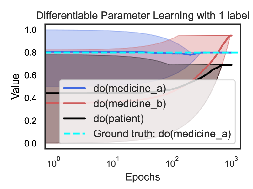
### Visual Description
## Line Chart: Differentiable Parameter Learning with 1 label
### Overview
This is a line chart with shaded confidence intervals, illustrating the learning progression of different causal parameters over training epochs. The chart compares the estimated values of three interventions against a known ground truth. The x-axis uses a logarithmic scale.
### Components/Axes
* **Title:** "Differentiable Parameter Learning with 1 label"
* **Y-axis:** Label is "Value". Scale is linear, ranging from 0.0 to 1.0 with major ticks at 0.0, 0.2, 0.4, 0.6, 0.8, and 1.0.
* **X-axis:** Label is "Epochs". Scale is logarithmic (base 10), with major ticks at 10⁰ (1), 10¹ (10), 10² (100), and 10³ (1000).
* **Legend:** Positioned in the bottom-right quadrant of the chart area, partially overlapping the data lines. It contains four entries:
1. `do(medicine_a)`: Solid blue line.
2. `do(medicine_b)`: Solid red line.
3. `do(patient)`: Solid black line.
4. `Ground truth: do(medicine_a)`: Cyan dashed line.
* **Data Series:** Each solid line is accompanied by a semi-transparent shaded area of the same color, representing a confidence interval or variance band.
### Detailed Analysis
**Trend Verification & Data Points (Approximate):**
* **`do(medicine_a)` (Blue Line):** Starts high (~0.8 at epoch 1), remains relatively flat with a slight dip around epoch 100 (~0.78), then rises sharply after epoch 100 to converge near ~0.95 by epoch 1000. The blue shaded confidence interval is very wide at the start (spanning ~0.4 to 1.0) and narrows significantly as epochs increase.
* **`do(medicine_b)` (Red Line):** Starts lower (~0.4 at epoch 1), shows a steady, accelerating upward trend. It crosses the blue line between epoch 100 and 1000 and converges to the same final value (~0.95) by epoch 1000. Its red shaded confidence interval widens considerably as epochs increase, especially after epoch 100.
* **`do(patient)` (Black Line):** Starts around ~0.45 at epoch 1, remains nearly flat until epoch 100, then increases to a final value of approximately ~0.7 by epoch 1000. Its black shaded confidence interval is narrow initially but widens notably in the later epochs.
* **`Ground truth: do(medicine_a)` (Cyan Dashed Line):** A constant horizontal line at y = 0.8 across all epochs.
**Spatial Grounding:** The legend is placed in the bottom-right, obscuring the lower portions of the rising red and black lines in the later epochs. The cyan ground truth line is clearly visible above the initial values of the red and black lines.
### Key Observations
1. **Convergence:** Both `do(medicine_a)` and `do(medicine_b)` converge to a value (~0.95) that is higher than the stated ground truth (0.8) for `do(medicine_a)`.
2. **Diverging Uncertainty:** The confidence intervals for `do(medicine_a)` and `do(medicine_b)` behave oppositely. Uncertainty for medicine_a decreases with more training, while uncertainty for medicine_b increases.
3. **Baseline Performance:** The `do(patient)` parameter, likely representing a baseline or control, shows the least improvement and ends at the lowest value.
4. **Learning Dynamics:** The most significant changes for all parameters occur after epoch 100 (10²), suggesting a critical phase in the learning process.
### Interpretation
This chart likely visualizes a causal inference or reinforcement learning experiment where an algorithm is learning the effect of different interventions (`do(medicine_a)`, `do(medicine_b)`) on a patient outcome, using limited labeled data (1 label).
* **What the data suggests:** The model successfully learns that both medicine interventions have a strong positive effect, eventually surpassing the known ground truth value for medicine_a. This could indicate model overestimation, or that the ground truth represents a different context. The steady rise of medicine_b suggests it is a viable alternative that the model learns to value equally.
* **Relationship between elements:** The ground truth serves as a benchmark. The patient line acts as a baseline. The crossing of the blue and red lines indicates a point in training where the model's estimate of medicine_b's effectiveness surpasses that of medicine_a.
* **Notable Anomalies:** The primary anomaly is the final estimated value for `do(medicine_a)` exceeding its own ground truth. The widening confidence interval for `do(medicine_b)` is also notable, suggesting the model becomes less certain about this parameter's value even as its mean estimate improves, possibly due to conflicting signals in the data. The chart demonstrates the model's ability to differentiate and learn distinct parameters, but also highlights potential issues with calibration or uncertainty quantification.
</details>
Figure 10: Value curve of three $\mathtt{do}$ operators during learning. With three targets (right) and with one target (left). The curves are averaged on 5 runs, with shaded area indicating the maximum and minimum value. (Best viewed in color)
## Appendix D Multi-Task Adaptation
<details>
<summary>x11.png Details</summary>
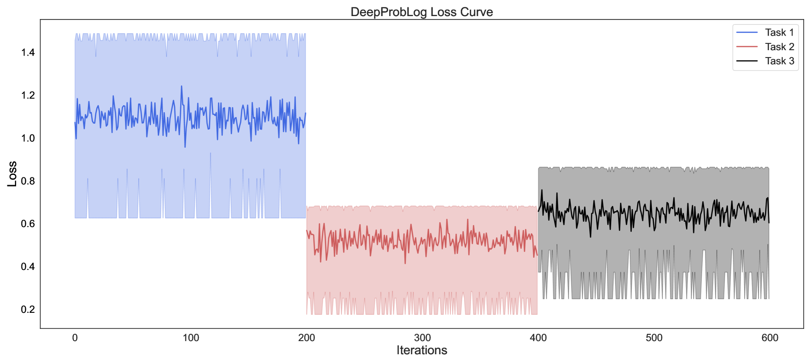
### Visual Description
## Line Chart: DeepProbLog Loss Curve
### Overview
This image is a line chart titled "DeepProbLog Loss Curve," displaying the training loss values for three distinct tasks over a series of iterations. The chart uses three colored lines, each with a corresponding shaded area, to represent the loss trajectory and its variability for each task.
### Components/Axes
* **Title:** "DeepProbLog Loss Curve" (centered at the top).
* **X-Axis:** Labeled "Iterations." The scale runs from 0 to 600, with major tick marks at 0, 100, 200, 300, 400, 500, and 600.
* **Y-Axis:** Labeled "Loss." The scale runs from 0.2 to 1.4, with major tick marks at 0.2, 0.4, 0.6, 0.8, 1.0, 1.2, and 1.4.
* **Legend:** Located in the top-right corner. It contains three entries:
* A blue line labeled "Task 1"
* A red line labeled "Task 2"
* A black line labeled "Task 3"
### Detailed Analysis
The chart presents three separate data series, each occupying a distinct segment of the iteration axis.
1. **Task 1 (Blue Line & Shaded Area):**
* **Spatial Grounding & Trend:** This series is plotted from iteration 0 to approximately 200. The blue line shows a highly volatile, noisy pattern with no clear upward or downward trend. It oscillates rapidly around a central value.
* **Data Points:** The central line fluctuates primarily between loss values of 1.0 and 1.2. The shaded blue area, representing the range or variance, extends from a lower bound of approximately 0.6 to an upper bound of approximately 1.5.
2. **Task 2 (Red Line & Shaded Area):**
* **Spatial Grounding & Trend:** This series is plotted from iteration 200 to 400. The red line also exhibits high-frequency noise but shows a very slight downward trend over its 200-iteration span.
* **Data Points:** The central line fluctuates primarily between loss values of 0.4 and 0.6. The shaded red area extends from a lower bound of approximately 0.2 to an upper bound of approximately 0.7.
3. **Task 3 (Black Line & Shaded Area):**
* **Spatial Grounding & Trend:** This series is plotted from iteration 400 to 600. The black line is similarly noisy but displays a slight upward trend over its duration.
* **Data Points:** The central line fluctuates primarily between loss values of 0.6 and 0.8. The shaded grey area extends from a lower bound of approximately 0.2 to an upper bound of approximately 0.9.
### Key Observations
* **Distinct Loss Regimes:** Each task operates within a clearly separated range of loss values. Task 1 has the highest loss (~1.1), Task 2 has the lowest (~0.5), and Task 3 is intermediate (~0.7).
* **High Variance:** All three tasks show significant variance (indicated by the wide shaded areas) around their mean loss, suggesting noisy training dynamics or inherent stochasticity in the tasks.
* **Sequential Training:** The tasks are trained sequentially, not concurrently, as their data series do not overlap on the iteration axis.
* **Trend Subtlety:** While all lines are noisy, Task 2 shows a subtle improvement (decreasing loss), and Task 3 shows a subtle degradation (increasing loss) over their respective training windows.
### Interpretation
The chart demonstrates the training progression of the DeepProbLog model on three different tasks. The data suggests that:
1. **Task Difficulty:** Task 2 appears to be the "easiest" for the model to learn, as it achieves and maintains the lowest loss value. Task 1 is the "hardest," with the highest loss.
2. **Training Stability:** The high variance across all tasks indicates that the training process is unstable or that the loss function has a lot of local noise. This could be due to factors like small batch sizes, a complex loss landscape, or the probabilistic nature of the model.
3. **Sequential Learning Behavior:** The model's performance does not carry over between tasks. When training switches from Task 1 to Task 2, the loss drops dramatically, and when it switches to Task 3, the loss increases again. This implies the model is likely being retrained or fine-tuned for each task from a similar starting point, rather than continually learning a joint representation.
4. **Potential Overfitting/Underfitting:** The slight upward trend in Task 3's loss could be an early sign of overfitting to that specific task's training data, or it could indicate that the model's capacity is being strained. The slight downward trend in Task 2 suggests continued, albeit slow, learning.
In summary, this loss curve provides a diagnostic view of a multi-task training regimen, highlighting differences in task difficulty, the noisy nature of the optimization process, and the compartmentalized learning of each task.
</details>
Figure 11: DeepProbLog [21] is initialized using the same candidate meta rules (also with randomized meta rule weights as NEMESYS). The loss curve is averaged on five runs, with the shadow area indicating the minimum and maximum number of the five runs. (Best viewed in color)
<details>
<summary>x12.png Details</summary>
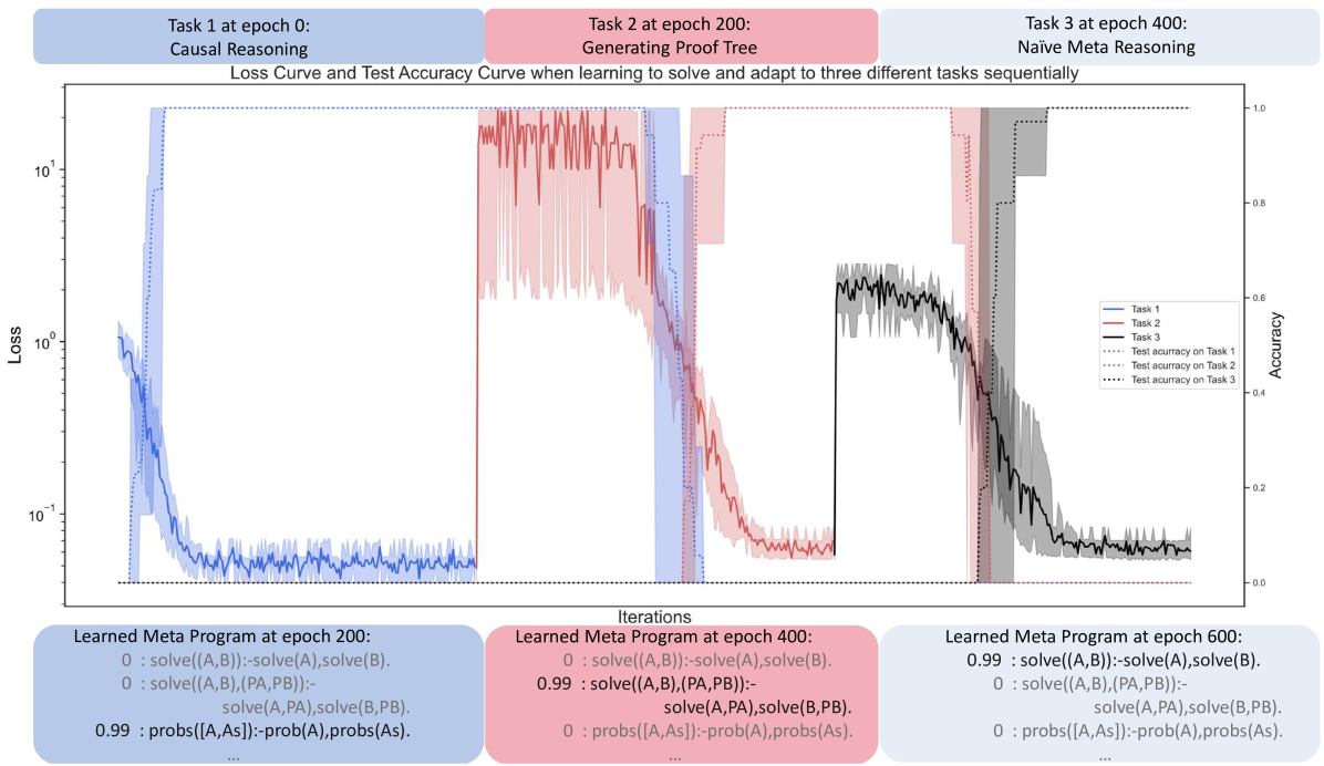
### Visual Description
## [Chart]: Loss Curve and Test Accuracy Curve for Sequential Task Learning
### Overview
The image is a technical chart illustrating the training process of a machine learning model as it sequentially learns three distinct tasks. It displays both the loss (error) and test accuracy over training iterations (epochs). The chart is divided into three vertical segments, each corresponding to the training period for a specific task. Below the main chart, three text boxes show the state of a "Learned Meta Program" at different epochs.
### Components/Axes
**Header (Top):**
- Three colored boxes label the tasks and their starting epochs:
- **Blue Box (Left):** "Task 1 at epoch 0: Causal Reasoning"
- **Pink Box (Center):** "Task 2 at epoch 200: Generating Proof Tree"
- **Grey Box (Right):** "Task 3 at epoch 400: Naive Meta Reasoning"
- **Chart Title:** "Loss Curve and Test Accuracy Curve when learning to solve and adapt to three different tasks sequentially"
**Main Chart Axes:**
- **X-axis (Bottom):** Label: "Iterations". Scale: Linear, from 0 to approximately 600 epochs. Major ticks at 0, 200, 400, 600.
- **Primary Y-axis (Left):** Label: "Loss". Scale: Logarithmic, ranging from 10⁻¹ (0.1) to 10¹ (10).
- **Secondary Y-axis (Right):** Label: "Accuracy". Scale: Linear, from 0.0 to 1.0.
**Legend (Center-Right):**
- Positioned inside the chart area, slightly right of center.
- **Solid Lines (Loss):**
- Blue solid line: "Task 1"
- Red solid line: "Task 2"
- Black solid line: "Task 3"
- **Dotted Lines (Accuracy):**
- Blue dotted line: "Test accuracy on Task 1"
- Red dotted line: "Test accuracy on Task 2"
- Black dotted line: "Test accuracy on Task 3"
- **Shaded Areas:** Each solid loss line has a corresponding shaded area of the same color, representing variance or confidence intervals.
**Footer (Bottom):** Three text boxes showing "Learned Meta Program" states.
- **Blue Box (Left):** "Learned Meta Program at epoch 200:"
- `0 : solve((A,B)):-solve(A),solve(B).`
- `0 : solve((A,B),(PA,PB)):- solve(A,PA),solve(B,PB).`
- `0.99 : probs([A,As]):-prob(A),probs(As).`
- **Pink Box (Center):** "Learned Meta Program at epoch 400:"
- `0 : solve((A,B)):-solve(A),solve(B).`
- `0.99 : solve((A,B),(PA,PB)):- solve(A,PA),solve(B,PB).`
- `0 : probs([A,As]):-prob(A),probs(As).`
- **Grey Box (Right):** "Learned Meta Program at epoch 600:"
- `0.99 : solve((A,B)):-solve(A),solve(B).`
- `0 : solve((A,B),(PA,PB)):- solve(A,PA),solve(B,PB).`
- `0 : probs([A,As]):-prob(A),probs(As).`
### Detailed Analysis
**Task 1 (Causal Reasoning) - Epochs 0-200 (Blue Region):**
- **Loss Trend:** The blue loss line starts high (≈1.0) and rapidly decreases within the first ~50 epochs, stabilizing at a low value (≈0.05-0.08) for the remainder of the period. The trend is a steep downward slope followed by a flat plateau.
- **Accuracy Trend:** The blue dotted accuracy line starts near 0.0 and rises sharply to near 1.0 (≈0.98) concurrently with the loss drop, remaining stable thereafter.
**Task 2 (Generating Proof Tree) - Epochs 200-400 (Pink Region):**
- **Loss Trend:** At epoch 200, the red loss line spikes dramatically to a high value (≈5-10). It exhibits high volatility (large spikes) for about 50-70 epochs before beginning a steady decline, reaching a low value (≈0.06-0.1) by epoch 400. The trend is a sharp spike, followed by noisy decline, then stabilization.
- **Accuracy Trend:** The red dotted accuracy line drops to near 0.0 at epoch 200. It recovers slowly, showing a gradual upward trend, reaching approximately 0.9 by epoch 400.
**Task 3 (Naive Meta Reasoning) - Epochs 400-600 (Grey Region):**
- **Loss Trend:** At epoch 400, the black loss line spikes to a moderate level (≈0.5-0.7). It shows a clear downward trend with moderate noise, decreasing to a low value (≈0.06-0.08) by epoch 600.
- **Accuracy Trend:** The black dotted accuracy line drops to near 0.0 at epoch 400. It recovers with a steady upward slope, reaching approximately 0.95 by epoch 600.
**Meta Program Evolution:**
- **Epoch 200:** The program with confidence `0.99` is `probs([A,As]):-prob(A),probs(As).` The two `solve` rules have confidence `0`.
- **Epoch 400:** The program with confidence `0.99` is `solve((A,B),(PA,PB)):- solve(A,PA),solve(B,PB).` The other two rules have confidence `0`.
- **Epoch 600:** The program with confidence `0.99` is `solve((A,B)):-solve(A),solve(B).` The other two rules have confidence `0`.
### Key Observations
1. **Sequential Learning & Catastrophic Forgetting:** The model successfully learns each new task, as evidenced by decreasing loss and increasing accuracy within each task's dedicated training period. However, the sharp spikes in loss and drops in accuracy for subsequent tasks at their start epochs (200, 400) indicate the model's parameters are being significantly adjusted, potentially interfering with previously learned knowledge.
2. **Task Difficulty/Adaptation Speed:** Task 1 is learned fastest. Task 2 shows the most volatile loss and a slower accuracy recovery, suggesting it may be more complex or cause more interference. Task 3 shows a smoother adaptation than Task 2.
3. **Meta-Program Specialization:** The "Learned Meta Program" boxes show that the model's internal rule confidence shifts dramatically between tasks. At each major epoch milestone (200, 400, 600), a different logical rule becomes dominant (confidence 0.99), while the others are suppressed (confidence 0). This suggests the model is reconfiguring its core reasoning strategy for each new task.
### Interpretation
This chart demonstrates a model undergoing **sequential multi-task learning**. The primary narrative is one of adaptation and specialization. The model is not simply accumulating knowledge; it is actively reconfiguring its internal "meta-program" (a set of logical rules) to prioritize the strategy most effective for the current task.
The **Peircean investigative** reading suggests the model is abductively reasoning about the best problem-solving framework for each new challenge. The shift from a `probs`-based rule (Task 1: Causal Reasoning) to a structured `solve` with proof trees (Task 2) and finally to a simpler, compositional `solve` (Task 3: Naive Meta Reasoning) indicates the model is discovering and adopting different "hypotheses" (rules) about how to reason.
The **notable anomaly** is the extreme volatility in Task 2's loss. This could indicate that "Generating Proof Tree" is a fundamentally different or more difficult task for the model's architecture, causing instability during the adaptation phase. The fact that the model stabilizes and achieves high accuracy by the end of each phase shows its robustness, but the interference at task boundaries highlights a key challenge in continual learning systems: balancing plasticity (learning new things) with stability (retaining old things). The meta-program shifts provide a window into *how* the model achieves this balance—by essentially "switching gears" its core reasoning engine.
</details>
Figure 12: Loss curve and accuracy curve of NEMESYS when learning to adapt to solve three tasks. NEMESYS solves three different tasks (causal reasoning, generating proof trees and naive meta reasoning) sequentially (each task is represented by a unique color encoding). The loss curve (solid line) and accuracy curve (dashed line) are averaged on five runs, with the shadow area indicating the minimum and maximum number of the five runs. For readability, the learned complete meta program is shown in the text. (Best viewed in color)
We also compute the accuracy on the test splits of three tasks during the learning process (Fig. 12 dashed line, color encoded). We choose DeepProbLog [21] as our baseline comparison method in this experiment, however, learning the weights of (meta) rules is not supported in DeepProbLog framework, thus we randomly initialized the weights of the meta rules and compute the loss (Fig 11).
In this paragraph, we provide the meta program learned by NEMESYS in the experiment. The weights of meta rules are color coded to visually represent how their values evolve during the learning process (the weights are provided at iteration $\mathtt{200}$ , $\mathtt{400}$ and $\mathtt{600}$ ), as illustrated in the accompanying Fig. 12.
| | $\displaystyle\hskip 6.45831pt\color[rgb]{0,0,1}0\ \hskip 4.30554pt\ \color[rgb ]{0.9,0.3608,0.3608}0.99\ \hskip 4.30554pt\ \color[rgb]{0,0,0}0\ :\mathtt{ solve(A,B)}\texttt{:-}\mathtt{solve(A),solve(B).}$ | |
| --- | --- | --- |