## End-to-End DNN Inference on a Massively Parallel Analog In Memory Computing Architecture
Nazareno Bruschi , Giuseppe Tagliavini , Angelo Garofalo , Francesco Conti
Irem Boybat , Luca Benini , Davide Rossi
∗ ∗ ∗† ∗ , ‡ ∗† ∗
University of Bologna , Bologna, Italy, ETH , Zurich, Switzerland
∗ † ‡ IBM Research , Zurich, Switzerland
Abstract -The demand for computation resources and energy efficiency of Convolutional Neural Networks (CNN) applications requires a new paradigm to overcome the 'Memory Wall'. Analog In-Memory Computing (AIMC) is a promising paradigm since it performs matrix-vector multiplications, the critical kernel of many ML applications, in-place in the analog domain within memory arrays structured as crossbars of memory cells. However, several factors limit the full exploitation of this technology, including the physical fabrication of the crossbar devices, which constrain the memory capacity of a single array. Multi-AIMC architectures have been proposed to overcome this limitation, but they have been demonstrated only for tiny and custom CNNs or performing some layers off-chip. In this work, we present the full inference of an end-to-end ResNet-18 DNN on a 512-cluster heterogeneous architecture coupling a mix of AIMC cores and digital RISCV cores, achieving up to 20.2 TOPS. Moreover, we analyze the mapping of the network on the available non-volatile cells, compare it with state-of-the-art models, and derive guidelines for next-generation many-core architectures based on AIMC devices.
Index Terms -In-Memory Computing, Heterogenous systems, many-core architectures, Convolutional Neural Networks
## I. INTRODUCTION
Matrix-Vector Multiplication (MVM) is the critical operation in modern Deep Neural Networks (DNN), and its optimization has been tackled from different perspectives, from software kernels to hardware accelerators. In recent years, Analog InMemory Computing (AIMC) has been a widely studied computing paradigm since it promises outstanding performance and energy efficiency on MVM operations [1]. However, the largescale usage of AIMC in commercial products is limited by technological issues, especially in fabricating large arrays. AIMC can be employed using very different memory technologies, which can be classified as volatile and non-volatile.
The former has a more mature community, especially for SRAM technology, due to its robustness and viability for largescale integration in any CMOS node. Several SRAM-based chips have been developed targeting any DNN requirements [2]. However, they generally require moving network parameters among large off-chip memories to be temporarily stored in the on-chip computational memory, negatively impacting energy consumption [3].
Non-volatile AIMC (nvAIMC) instead merges parameter storage with computational memory. In this way, parameters do not need to be transferred from onor off-chip storage through the memory hierarchy. However, the limited writing access speed [4] of nvIMC devices introduces the need for a static mapping strategy to preserve the performance capability of such devices. Moreover, a further challenge is the fabricable size of nvIMC devices, which de-facto is limited to 1024 × 1024 with up to 8-bit equivalent memory cells [4].
During the last few years, the fabrication of several prototypes exploiting these technologies [5]-[7] demonstrated the feasibility of the approach, despite several open challenges related to the intrinsic variability of analog computing, the need for specialized training to address analog noise and nonidealities. On the other hand, most of these works aimed at demonstrating the technology rather than targeting end-to-end inference of deep neural networks. One of the limitations of nvAIMC cores is their little flexibility due to the ability to implement only MVMs.
For this reason, few recent works [8]-[10] proposed the integration of nvAIMC cores into digital System-on-Chips (SoC), exploiting a mix of nvAIMC cores and more flexible specialized and programmable digital processors. Thanks to this mix, they demonstrated remarkable performance on the full inference of neural networks in the mobile domain, such as MobileNetV2, time multiplexing computations on several nvAIMC cores [9], [10]. Indeed, in the mobile domain, it is common that only one sample is processed at a time, relaxing the requirements of layer pipelining. This constraint significantly limits the potential of nvAIMC since only one core can be active at a given time.
This constraint can be relaxed when leaving the mobile domain: high-performance inference of DNNs typically exploits batching due to the large number of images typically processed in HPC and data centers applications. Several recent works exploited this feature proposing many-core data-flow architectures. On the other hand, most of these works made strong assumptions about the characteristics of the networks to be processed to better fit the shape of the DNN on the proposed architectures. For example, Dazzi et al. [11] targeted a relatively small ResNet-like network targeting the CIFAR10 dataset, while Shafiee et al. [12] and Ankit et al. [13] target VGG-like networks featuring no residual layers, nicely fitting mapping on pipelined data-flow architectures. However, DNNs generally feature data flow graph loops (e.g., residual layers) that make a straightforward pipelining implementation much more challenging. Moreover, most of these architectures only feature specialized accelerators for implementing digital functions such as ReLU, and MaxPool, somehow limiting the flexibility of their approach.
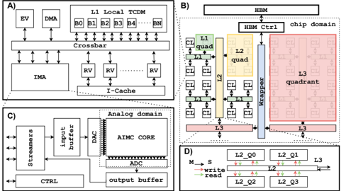
Fig. 1. A) Cluster architecture. B) Massively parallel system architecture. C) IMA subsystem. D) Router model.
<details>
<summary>Image 1 Details</summary>
### Visual Description
\n
## Diagram: System Architecture Overview
### Overview
The image presents a set of four diagrams (A, B, C, and D) illustrating the architecture of a complex system, likely a specialized processor or accelerator. Diagram A shows the processing core, B depicts the memory hierarchy, C illustrates the analog domain, and D details the memory access scheme. The diagrams are interconnected through data flow and control signals.
### Components/Axes
The diagrams do not have traditional axes. Instead, they are block diagrams with labeled components and connections. Key components include:
* **Diagram A:** EV, DMA, L1 Local TCDM (B0, B1, B2, B3, B4, BN), Crossbar, IMA, RV (repeated three times), I-Cache.
* **Diagram B:** HBM, HBM Ctrl, chip domain, L1 quad, L2 quad, L3 quadrant, wrapper, CL (repeated multiple times), EF (repeated multiple times).
* **Diagram C:** Streamers, input buffer, DAC, AIMC CORE, ADC, output buffer, CTRL.
* **Diagram D:** S, L2, Q0, Q1, Q2, Q3, read, write.
### Detailed Analysis or Content Details
**Diagram A: Processing Core**
* **EV** and **DMA** feed into the **L1 Local TCDM**, which is divided into blocks B0 through BN (approximately 5 blocks shown, with BN indicating more).
* The **L1 Local TCDM** is connected to a **Crossbar** which then connects to the **IMA** and multiple **RV** units (three shown).
* The **IMA** and **RV** units connect to the **I-Cache**.
* Arrows indicate data flow between these components.
**Diagram B: Memory Hierarchy**
* **HBM** (High Bandwidth Memory) is controlled by **HBM Ctrl**.
* The **HBM** connects to the **chip domain**, which contains **L1 quad**, **L2 quad**, and **L3 quadrant**.
* The **L1 quad** and **L2 quad** are interconnected via **CL** and **EF** connections.
* The **L2 quad** connects to the **L3 quadrant** via a **wrapper**.
* The **L3 quadrant** is a large block with internal structure.
**Diagram C: Analog Domain**
* **Streamers** feed into an **input buffer**.
* The **input buffer** connects to a **DAC** (Digital-to-Analog Converter).
* The **DAC** feeds into the **AIMC CORE**.
* The **AIMC CORE** connects to an **ADC** (Analog-to-Digital Converter).
* The **ADC** outputs to an **output buffer**.
* **CTRL** signals control the flow.
**Diagram D: Memory Access Scheme**
* **S** (Start) signal initiates a memory access.
* **L2** is the primary memory level shown.
* **Q0, Q1, Q2, Q3** represent memory queues or partitions within L2.
* Arrows indicate **read** and **write** operations to the queues.
* The diagram shows a sequence of operations involving the queues.
### Key Observations
* The system employs a hierarchical memory structure (HBM, L1, L2, L3).
* There is a clear separation between the processing core (A), memory hierarchy (B), and analog domain (C).
* The memory access scheme (D) suggests a queuing mechanism for handling read and write requests.
* The use of "quad" and "quadrant" suggests a tiled or partitioned architecture.
* The diagram does not provide specific numerical values or performance metrics.
### Interpretation
The diagrams depict a highly parallel and specialized processing system. The architecture is designed for high-bandwidth data processing, likely involving analog computation (AIMC CORE) and efficient memory access. The separation of the analog domain suggests a hybrid digital-analog approach. The queuing mechanism in the memory access scheme (D) is likely implemented to manage concurrent read and write requests to the memory hierarchy, optimizing performance. The use of multiple RV units in Diagram A suggests a vector or SIMD processing capability. The overall system appears to be optimized for applications requiring high throughput and low latency, such as machine learning or signal processing. The lack of specific values makes it difficult to assess the system's performance characteristics quantitatively. The diagrams provide a high-level overview of the architecture, and further details would be needed to understand the specific implementation and capabilities of the system.
</details>
In this work, we tackle the problem from another perspective. We present a general-purpose system based on RISC-V cores for digital computations and nvAIMC cores for analogamenable operations, such as 2D convolutions. A scalable hierarchical network-on-chip interconnects the system to maximize on-chip bandwidth and reduce communication latency. We evaluate all the system inefficiencies, especially for the nonideal mappings and communication infrastructure bottleneck running a real-life network for state-of-the-art applications such as ResNet-18 inference on 256 × 256 image dataset. We perform an experimental assessment on an extended version of an opensource system-level simulator [14], resulting in up to 20.2 TOPS and 6.5 TOPS/W for the whole ResNet-18 inference of a batch of 16 256x256 images in 4.8 ms. The hardware and software described in this work are open-source, intending to support and boost an innovation ecosystem for next-generation computing platforms.
## II. MASSIVELY PARALLEL HETEROGENEOUS SYSTEM ARCHITECTURE
This section presents the proposed heterogeneous manycore SoC architecture. It consists of multiple heterogeneous (analog/digital) clusters communicating through a hierarchical AXI interconnect gathering data from a shared High-Bandwith Memory (HBM), as shown in Fig. 1B.
1) Cluster : The core of the proposed system architecture consists of heterogeneous analog/digital clusters (Fig. 1A). Each cluster contains a set of RISC-V cores (CORES) [15], a shared multi-bank scratchpad data memory (L1) enabling Single Program Multiple Data (SPMD) computations, a hardware synchronizer to accelerate common parallel programming primitives such as thread dispatching and barriers, and a DMA for the cluster to cluster and cluster to HBM communication. Each cluster also includes a nvAIMC Accelerator (IMA) sharing the same multi-banked memory as the CORES for efficient communication, similarly to the architecture presented in Garofalo et al. [9].
2) IMA : The IMA is built around a Phase-Change Memory (PCM) computational memory organised as a 2D array featuring horizontal word lines and vertical bit lines (Fig. 1C). In computational memory, the PCM cells are exploited as
TABLE I
## GVSOC ARCHITECTURE PARAMETERS
| Parameter | Value |
|---------------------------------------------|------------------------|
| Number of clusters | 512 |
| Number of IMA per cluster | 1 |
| Number of CORES per cluster | 16 |
| L1 memory size | 1 MB |
| HBM size | 1.5 GB |
| Operating frequency | 1 GHz |
| Number of streamers ports (read and write) | 16 |
| IMA crossbar size | 256 × 256 |
| Analog latency (MVM operation) | 130 ns |
| Quadrant factor (HBM link,wrapper,L3,L2,L1) | (1,8,4,4,4) |
| Data Width (HBM link,wrapper,L3,L2,L1) | (64,64,64,64,64) Bytes |
| Latency (HBM, link,wrapper,L3,L2,L1) | (100,4,4,4,4) cycles |
programmable resistors placed at the cross points between the word lines and the bit lines, which allows the implementation of MVM in the analog domain with high parallelism and efficiency. In this work, we assume an MVM to be executed in 130 ns as reported in Khaddam et al. [7]. At the beginning of each word lines and the end of each bit lines , Digital-toAnalog (DAC) and Analog-to-Digital converters (ADC) converters perform the conversion between analog and digital domains, respectively. ADCs and DACs connect to two digital buffers connected to the L1 memory through a set of streamers featuring programmable address generation.
- 3) Interconnect : The interconnect infrastructure connecting the clusters in the proposed many-core architecture consists of a highly parametrizable hierarchical network composed of a set of AXI4 nodes , as proposed in Kurth et al. [16]. The network topology specifies different regions called quadrants connecting groups of clusters: the Level 1 nodes connect N 1 quadrants (clusters), the Level 2 nodes connect N 2 Level 1 quadrants, and the Level Level N nodes connect N N Level N-1 quadrants, as shown in Fig. 1B. The Quadrant Factor for a given level N defines the number of quadrants (either clusters or level N-1 quadrants) connected to the AXI node for each level. Clusters feature a master and a slave port, which means that a transaction can either be initiated by the target cluster through its master port or by any other cluster through the target cluster's slave port. The same concept applies to the whole hierarchy of quadrants. In both cases, transactions can be either read or write transactions with full support for bursts according to AXI4 specifications. The last level of the interconnect architecture, called Wrapper, connects all the levels below to the off-chip HBM through an HBM controller.
## III. SIMULATION INFRASTRUCTURE
We modeled the proposed architecture by extending an opensource simulator named GVSOC [14] meant to simulate RISCV-based clustered multi-core architectures. It is a C++ eventbased simulator featuring a simulation speed of 25 MIPS and an accuracy of more than 90% compared to a cycle-accurate equivalent architecture when simulating a full DNN in a single cluster, as reported in Bruschi et al. [14].
The main components integrated into the simulator are the IMA and the interconnect infrastructure extending the capabili-
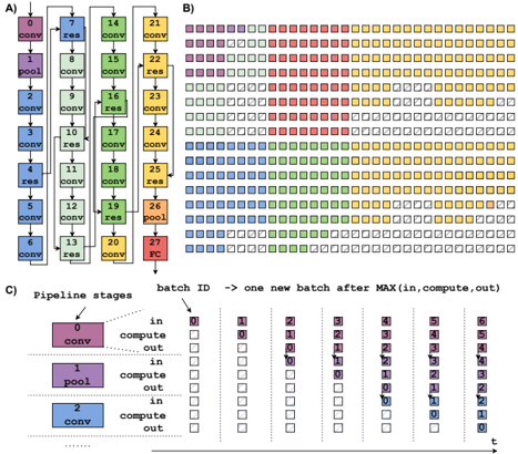
Fig. 2. A) Directed Acyclic Graph (DAG) of the ResNet-18 execution. B) Mapping example on 512 clusters. C) High-level description of pipelining computational model.
<details>
<summary>Image 2 Details</summary>
### Visual Description
\n
## Diagram: Convolutional Neural Network Pipeline Visualization
### Overview
The image presents a visualization of a convolutional neural network (CNN) pipeline, broken down into three parts (A, B, and C). Part A shows the network architecture with labeled layers. Part B displays a heatmap-like representation of batch processing across pipeline stages. Part C details the pipeline stages and their activity over time with a table.
### Components/Axes
**Part A: Network Architecture**
* Layers: "conv" (convolutional), "res" (residual), "pool" (pooling), "FC" (fully connected).
* Nodes are numbered 1 through 27.
* Connections indicate data flow.
**Part B: Batch Processing Heatmap**
* X-axis: "batch ID" – representing sequential batches processed. The arrow indicates that each batch represents the maximum of "in, compute, out".
* Y-axis: Rows represent individual processing units or stages.
* Colors: Represent the stage of processing (likely "in", "compute", "out"). The legend is implicit in the color scheme.
* Red: Likely "in"
* Yellow: Likely "compute"
* Blue: Likely "out"
* Green: Likely "compute"
**Part C: Pipeline Stages Table**
* Pipeline Stages: 0, 1, 2.
* Stage 0: "conv"
* Stage 1: "pool"
* Stage 2: "conv"
* Columns: Represent time steps (batch IDs) from 0 to 6.
* Rows: Indicate the state of each pipeline stage ("in", "compute", "out") at each time step.
* Colors: Correspond to the pipeline stage state.
* Red: "in"
* Yellow: "compute"
* Blue: "out"
### Detailed Analysis or Content Details
**Part A: Network Architecture**
The network consists of a series of convolutional, residual, pooling, and fully connected layers. The layers are arranged in a sequential manner.
* Nodes 1-3: "conv"
* Node 4: "res"
* Nodes 5-7: "conv"
* Node 8: "pool"
* Nodes 9-11: "conv"
* Node 12: "res"
* Nodes 13-15: "conv"
* Node 16: "pool"
* Nodes 17-19: "conv"
* Node 20: "res"
* Nodes 21-23: "conv"
* Node 24: "pool"
* Nodes 25-27: "conv"
* Node 27: "FC"
**Part B: Batch Processing Heatmap**
The heatmap shows the activity of different processing units over time.
* The heatmap is approximately 15 rows by 7 columns.
* The first few columns (batch IDs 0-2) show predominantly red ("in") states.
* As the batch ID increases, yellow ("compute") and blue ("out") states become more prevalent.
* There is a staggered pattern of activity, indicating pipelining.
* The heatmap shows a repeating pattern of activity across batches.
**Part C: Pipeline Stages Table**
The table details the state of each pipeline stage at each time step.
* Stage 0 ("conv"):
* Batch 0: "in" (red)
* Batch 1: "compute" (yellow)
* Batch 2: "out" (blue)
* Batch 3-6: "in" (red)
* Stage 1 ("pool"):
* Batch 0: "in" (red)
* Batch 1: "out" (blue)
* Batch 2: "in" (red)
* Batch 3: "compute" (yellow)
* Batch 4: "out" (blue)
* Batch 5-6: "in" (red)
* Stage 2 ("conv"):
* Batch 0: "in" (red)
* Batch 1: "in" (red)
* Batch 2: "compute" (yellow)
* Batch 3: "out" (blue)
* Batch 4: "in" (red)
* Batch 5: "compute" (yellow)
* Batch 6: "out" (blue)
### Key Observations
* The pipeline operates in a staged manner, with each stage processing data sequentially.
* The heatmap in Part B visually demonstrates the pipelining effect, where multiple batches are in different stages of processing simultaneously.
* The table in Part C confirms the pipelining behavior, showing how each stage transitions between "in", "compute", and "out" states over time.
* The network architecture in Part A provides the structural context for the pipeline visualization.
### Interpretation
The image illustrates the concept of pipelining in a CNN. Pipelining allows for increased throughput by overlapping the execution of different stages of the network. The heatmap and table in Parts B and C provide a visual and tabular representation of how data flows through the pipeline, with each batch progressing through the stages concurrently. The staggered activity patterns demonstrate that while one batch is being processed in one stage, another batch may be in a different stage. This parallel processing significantly improves the efficiency of the CNN. The network architecture in Part A shows the layers that are being pipelined. The color coding consistently represents the state of each stage, making it easy to understand the flow of data. The diagram effectively communicates the benefits of pipelining in CNNs, highlighting how it enables faster and more efficient processing of data.
</details>
ties of the simulator towards many-core accelerators (i.e., up to 512 clusters and 8192 RISC-V cores). The IMA is integrated into the cluster as a master of the cluster crossbar. All the components of the IMA have been modeled, including the input and output buffers and the streamers. At the system level, the interconnect infrastructure has been modeled as a set of parametric router components with configurable data width, latency, and the number of master and slave ports combined together to create the topology described in Fig. 1D. Table I describes the configuration parameters of the platform used in this work. All the modules in the simulator have been calibrated using the cycle-accurate RTL and FPGA equivalent. 256 × 256 IMA size has been used since it has been demonstrated in more works and shows better technological feasibility at this time [7]. This infrastructure allows to simulate the execution of a full ResNet-18 on 512 instantiated clusters in less than 20 minutes on a 32 GB RAM, Intel(R) Core(TM) i7-2600 CPU @ 3.40GHz.
## IV. COMPUTATIONAL MODEL
This section presents the computational model of the proposed massively parallel heterogeneous architecture, detailing its main characteristics: Layer Mapping, IMA execution, Pipelining, Data Tiling, and Self-Timed Execution Flow.
- 1) Static Layer Mapping : According to the computational model of the proposed many-core architecture, each layer of a DNN is statically mapped to a certain number of clusters, while the input/output features maps (IFM/OFM) are streamed from producer to consumer clusters. Fig. 2B shows the mapping of the ResNet-18 on the architecture, where each node of the graph in Fig. 2A represents a CNN layer, grouped by color according to the IFM dimensions, and every layer is mapped on different clusters of the system, as shown in Fig. 2B. The number of clusters used to map a specific layer depends on the number of
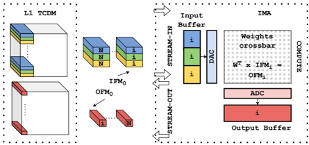
Fig. 3. IMA execution model.
<details>
<summary>Image 3 Details</summary>
### Visual Description
\n
## Diagram: L1 TCDM and IMA Architecture
### Overview
The image depicts a diagram illustrating the architecture of an L1 TCDM (Third-Order Correlation Detector Memory) and its interface with an IMA (In-Memory Accelerator). The diagram shows the data flow from the L1 TCDM to the IMA, highlighting the input buffering, weight crossbar, computation, and output buffering stages. The diagram uses color-coding to represent different data elements and stages.
### Components/Axes
The diagram is divided into two main sections: L1 TCDM (left) and IMA (right).
* **L1 TCDM:** Shows a 3D representation of memory blocks with colored layers. Labels include "L1 TCDM", "IFM₀", "OFM₀", and "i" and "N" within the blocks.
* **IMA:** Contains components labeled "Input Buffer", "Weights crossbar", "COMPUTE", "ADC", and "Output Buffer". Arrows indicate data flow labeled "STREAM-IN" and "STREAM-OUT".
* **Equation:** "Wᵀ x IFM₀ = OFM₀" is present within the "Weights crossbar" section.
* **Color Coding:**
* Blue: Represents input data "i".
* Yellow: Represents data "N".
* Red: Represents output data.
* Gray: Represents the structure of the memory blocks.
### Detailed Analysis or Content Details
**L1 TCDM:**
* The L1 TCDM shows a series of stacked blocks. The top block has layers colored blue, yellow, and blue. The bottom block has layers colored red.
* The label "IFM₀" points to the blue and yellow blocks, indicating the input feature map.
* The label "OFM₀" points to the red blocks, indicating the output feature map.
* The letters "i" and "N" are present within the blocks, likely representing data elements or indices.
**IMA:**
* **Input Buffer:** Contains three stacked blocks colored blue, labeled "i". A "DAC" (Digital-to-Analog Converter) is also present.
* **Weights Crossbar:** A grid-like structure labeled "Weights crossbar" is shown. The equation "Wᵀ x IFM₀ = OFM₀" is embedded within this section, indicating a matrix multiplication operation.
* **ADC:** An "ADC" (Analog-to-Digital Converter) is present after the "Weights crossbar".
* **Output Buffer:** Contains a single red block labeled "i".
**Data Flow:**
* "STREAM-IN" arrows point from the L1 TCDM to the Input Buffer.
* "STREAM-OUT" arrows point from the Output Buffer.
* The data flow within the IMA is sequential: Input Buffer -> Weights Crossbar -> ADC -> Output Buffer.
### Key Observations
* The diagram illustrates a data flow from the L1 TCDM to the IMA for performing a matrix multiplication operation.
* The use of color-coding helps to visualize the different data elements and stages of the process.
* The equation "Wᵀ x IFM₀ = OFM₀" highlights the core computation performed by the IMA.
* The diagram focuses on the architectural components and data flow rather than specific numerical values.
### Interpretation
The diagram demonstrates an architecture for accelerating computations by leveraging in-memory processing. The L1 TCDM serves as a memory block holding input and output feature maps (IFM₀ and OFM₀). The IMA performs a matrix multiplication (Wᵀ x IFM₀) using a weights crossbar, converting data between digital and analog domains using DAC and ADC, and storing the result in an output buffer. The STREAM-IN and STREAM-OUT arrows indicate the data transfer between the memory and the accelerator. This architecture aims to reduce data movement, which is a major bottleneck in traditional computing systems, by performing computations directly within the memory. The use of "i" and "N" within the memory blocks suggests indexing or data partitioning schemes. The diagram is a high-level representation of the system and does not provide details on the specific implementation of the components or the size of the data elements. It is a conceptual illustration of a potential hardware architecture for efficient machine learning or signal processing applications.
</details>
parameters of the layer. For example, Layer 22 features 2.3M parameters, requiring 40 clusters for the mapping, assuming each 256x256 IMA can store 64K parameters.
- 2) IMA Execution : As described in Sec. II, the IMA subsystem communicates directly to the L1 of the cluster, acting as a master of the TCDM interconnect. Assuming DNN parameters of a specific layer are being pre-loaded to the nonvolatile array, IMA execution is composed of three distinct phases, as shown in Fig. 3. Stream-in fetches the IFM of the layer and moves them to the input buffer of the IMA. Compute performs the input data conversion by the DACs, the analog MVM execution on the crossbar, and the ADCs conversion. Stream-out moves the output digital MVM result from the output buffers to the L1 memory. Input and output buffers are duplicated to enable double buffering, completely overlapping the cost of transfers between the L1 and the buffers with the computation, maximizing the computational efficiency of the accelerator.
- 3) Pipelining : When the inference starts, the IFM of the first layer is streamed into the first set of clusters which process it generating the OFM, which is then passed to the second set of clusters and so on. Assuming the possibility of having large batches of images allows for the creation of the software pipeline described in Fig. 2C, where different chunks of data are processed by a different set of clusters simultaneously, fully overlapping the data movements (i.e., in charge of the DMA) with the computation (i.e., in charge of IMA and/or CORES). Ensuring that all pipeline stages execute in the same amount of time is essential when creating such a pipeline structure. Techniques to speed-up pipeline stages, such as parallelization and data-replication , will be discussed in Sec. V.
- 4) Data Tiling : To fit IFM/OFM of large DNN models within the limited memory resources of the clusters (1 MB of L1 memory is assumed in this work), we split IFM/OFM into smaller chunks of data called tiles , processed by the clusters as soon as the input data is transferred to the L1 memory. In particular, data tiling is always performed along the W in and W out dimensions for input and output, respectively. In this work, we assume a static tiling strategy, and W in/out implicitly defines the batching dimension. Therefore, the batches are composed of vertical slices of IFM/OFM. The other dimensions ( C in and H in ) are, when necessary, tiled in other clusters to fit the memory requirements (parameters mapping) or to speed up the computation ( parallelization ).
- 5) Self-Timed Execution : To implement the pipeline between the tiled structure described in IV-4, we exploit a dataflow self-timed execution model. Computation in a cluster can be performed by the CORES, IMA, or both in parallel. While software execution on the CORES is synchronous, IMA execution is managed asynchronously (like DMA transfers). A cluster can perform a certain computation whenever three conditions are satisfied: a) Chunk N+1 from the producers can be loaded to the L1 memory, b) the consumers are ready to accept the output data of chunk N-1, c) both IMA and CORES are free to compute chunk N. If all the conditions are satisfied, the new iteration can start with the following execution flow: 1) the CORE0 (i.e., master core) first waits for the events from the input and output DMA channels and IMA, 2) the CORE0 configures and triggers I/O DMA channels and IMA for computation of next tile 3) digital processing is performed in parallel on the CORES. 4) All the CORES go to sleep, waiting for the events described in point 1).
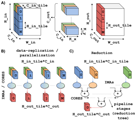
Fig. 4. A) Generic layer IFM, parameters and OFM. B) Data-replication and parallelization . C) Reduction operation.
<details>
<summary>Image 4 Details</summary>
### Visual Description
\n
## Diagram: Tiling and Parallelization Scheme for Convolutional Neural Networks
### Overview
The image presents a diagram illustrating a tiling and parallelization scheme for convolutional neural networks (CNNs). It depicts how input data is divided into tiles, processed in parallel, and then reduced to produce the output. The diagram is divided into three sections: A) Tiling, B) Data Replication/Parallelization, and C) Reduction.
### Components/Axes
The diagram uses several labels to describe the dimensions and processes involved:
* **A) Tiling:**
* `H_in`: Input Height
* `W_in`: Input Width
* `C_in`: Input Channels
* `H_out`: Output Height
* `W_out`: Output Width
* `C_out`: Output Channels
* `H_in_tile`: Height of input tile
* `H_out_tile`: Height of output tile
* `K`: Kernel size (indicated by the double-headed arrow)
* Numbers 0 through N and 0 through M are used to label tiles within the input and output volumes, respectively.
* **B) Data Replication / Parallelization:**
* `IMAs / CORES`: Indicates the mapping of input tiles to processing cores.
* `H_in_tile * C_in`: Dimensions of the input tile.
* `H_out_tile * C_out`: Dimensions of the output tile.
* Labels i, j, and M are used to identify specific tiles and their corresponding cores.
* **C) Reduction:**
* `IMAs`: Intermediate results.
* `CORES`: Processing cores.
* `pipeline stages (tree)`: Indicates a tree-like structure for the reduction process.
* `H_in_tile * C_in_tile`: Dimensions of the input tile.
* `H_out_tile * C_out`: Dimensions of the output tile.
* Plus signs (+) indicate summation operations.
### Detailed Analysis or Content Details
**A) Tiling:**
This section shows the division of an input volume into tiles. The input volume has dimensions `H_in`, `W_in`, and `C_in`. It is divided into tiles of size `H_in_tile` along the height and `W_in` along the width. The number of tiles along the height is represented by `N`. The output volume has dimensions `H_out`, `W_out`, and `C_out`. It is divided into tiles of size `H_out_tile` along the height and `W_out` along the width. The number of tiles along the height is represented by `M`. A kernel of size `K` is used for the convolution operation.
**B) Data Replication / Parallelization:**
This section illustrates how the input tiles are replicated and distributed to multiple cores for parallel processing. Each core processes one input tile and produces one output tile. The input tiles are labeled 0 through N, and the output tiles are labeled 0 through M. The mapping between input tiles and cores is indicated by the lines connecting the tiles to the cores.
**C) Reduction:**
This section shows the reduction process, where the intermediate results from the cores are combined to produce the final output. The intermediate results are represented by the `IMAs`. The cores perform summation operations to combine the intermediate results. The reduction process is organized in a tree-like structure, with multiple pipeline stages.
### Key Observations
* The tiling scheme divides the input and output volumes into smaller tiles to facilitate parallel processing.
* The data replication/parallelization scheme distributes the input tiles to multiple cores for parallel processing.
* The reduction scheme combines the intermediate results from the cores to produce the final output.
* The pipeline stages in the reduction scheme suggest a multi-stage processing pipeline.
### Interpretation
The diagram demonstrates a strategy for accelerating convolutional neural network computations through tiling and parallelization. By dividing the input data into smaller tiles, the computation can be distributed across multiple processing cores, significantly reducing the overall processing time. The reduction stage efficiently combines the results from these cores to produce the final output. The tree-like structure of the reduction stage suggests a hierarchical approach to combining the intermediate results, potentially optimizing communication and synchronization between cores. This approach is particularly relevant for large-scale CNNs where computational demands are high. The use of "IMAs" suggests intermediate activation maps. The diagram highlights a common technique used in hardware acceleration of deep learning models, where the workload is partitioned and distributed to maximize throughput.
</details>
## V. EVALUATION: RESNET-18
In this section, we present the mapping of the ResNet-18 on the proposed many-core architecture, providing insights on the adaptations required to the baseline mapping and execution model presented in Sec. IV to map all the layers and balance the pipeline optimally. The key operation of a ResNet-18 is a sequence of two 3x3 2D convolutions followed by a tensor addition (i.e., residual layer) between the OFM of the previous layer and the OFM of the previous residual layer. The first two layers are a 7x7 2D convolution followed by a MaxPool activation layer that starts propagating the residuals. The topology is shown in Fig. 2A.
- 1) Multi-cluster layers : When mapping a real-life network to the many-core architecture, the ideal condition would consist of perfectly matching the parameters of every layer with the size of the IMA. Unfortunately, this is not the case in the most
2. general case. Two types of situations might arise, depending on the dimension of the IFM/OFM. When the size of the input channels multiplied by the kernel size ( C in × K x × K y ) is greater than the number of rows of the IMA (i.e., 256), multiple IMAs are needed to compute the partial outputs. Then, a reduction among these partial outputs has to be performed to compute the OFM. On the other hand, while the size of the output channels is larger than the number of columns of the IMA (i.e., 256), the inputs need to be broadcasted to all the IMA involved (storing a different set of output channels parameters), and multiple IMAs compute part of the output channels at the same time. In some layers of ResNet-18, the two situations arise concurrently. This mapping approach has to be applied to all the layers computed in the analog domain, excluding Layer 0 .
- 2) Data-replication and Parallelization : In a pipelined computational model, the throughput of the whole pipeline is limited by the latency of the slowest stage. Hence, the pipeline has to be balanced as much as possible to achieve high throughput. Unbalancing might depend on many causes, and we will explain some of them in Sec. VI. A technique to speed up the execution of layers (i.e., one stage of the pipeline) executed in the analog domain (i.e., on the IMA) is data-replication . Data-replication increases the parallelism, replicating the parameters of a layer on different IMAs and computing at the same time multiple jobs on multiple chunks of the IFM. With this approach, the speed-up, net of overheads due to communication and data tiling, is theoretically equal to the number of replications at the cost of area, as the same layer parameters are stored on multiple IMAs (Fig. 4B). In this work, we extensively use this technique, especially for the first layers of the network. If the bottleneck of the pipeline is a layer executed in the digital domain (e.g., residual, reductions, pooling), one option is to parallelize the computation on the CORES over multiple clusters. A plain parallelization scheme is used for pooling and residual layers (i.e., Layers 1, 4, 7, 13, 19).
- 3) Reduction Management : A different approach has to be adopted for the reduction since this operation requires a hierarchical tree (Fig. 4C) featuring limited and decreasing parallelism. In particular, the level of parallelism of this operation is implicit in the structure of the network. In ResNet18, we might have to sum up the partial products of up to 20 clusters (i.e., Layers 20-21, 23-24) according to the multicluster mapping strategy described in Sec. V-1. In this context, the computation of the residuals might form a bottleneck for the pipeline since this operation has to be performed by the CORES in the digital domain. To accelerate these layers we split the hierarchical tree into several pipeline stages and assign each pipeline stage to a logarithmically decreasing number of clusters with well-balanced latency. This approach has been exploited in all reduction layers.
- 4) Residuals Management : In an ideal pipelined data flow, data are exchanged only among consecutive pipeline stages. On the other hand, in many modern DNNs such as ResNet18, this is not the case due to the presence of residual layers.
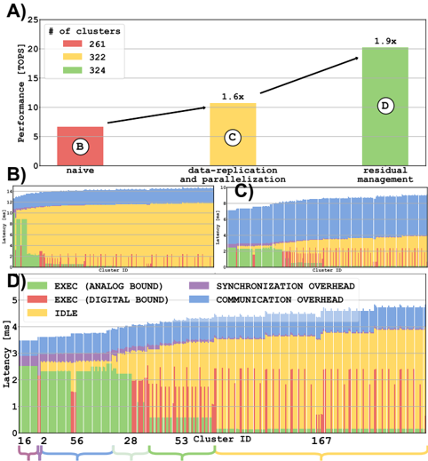
Fig. 5. ResNet-18 inference results. A) Throughput with different mapping optimizations. B) Execution time on every cluster in naive implementation. C) Execution time on every cluster in data-replication and parallelization implementation. D) Execution time on every cluster in final implementation.
<details>
<summary>Image 5 Details</summary>
### Visual Description
## Bar Chart with Stacked Area Charts: Performance Comparison of Different Approaches
### Overview
The image presents a performance comparison of three different approaches: "naive", "data-replication and parallelization", and "residual management". The performance is measured in TOPS (Tera Operations Per Second). The top portion (A) is a bar chart showing the performance of each approach. The bottom portion (B, C, D) consists of stacked area charts that break down the latency for each approach across different cluster IDs.
### Components/Axes
* **Top Chart (A):**
* X-axis: Approaches - "naive", "data-replication and parallelization", "residual management".
* Y-axis: Performance [TOPS], ranging from 0 to 25.
* Legend:
* Red: # of clusters = 261
* Yellow: # of clusters = 322
* Green: # of clusters = 324
* **Bottom Charts (B, C, D):**
* X-axis: Cluster ID, ranging from 0 to approximately 167.
* Y-axis: Latency [ms], ranging from 0 to 5.
* Legend:
* Green: EXEC (ANALOG BOUND)
* Yellow: EXEC (DIGITAL BOUND)
* Red: IDLE
* Blue: SYNCHRONIZATION OVERHEAD
* Gray: COMMUNICATION OVERHEAD
### Detailed Analysis or Content Details
**Top Chart (A):**
* **Naive:** Performance is approximately 5.2 TOPS (red bar).
* **Data-replication and parallelization:** Performance is approximately 8.3 TOPS (yellow bar). This is a 1.6x improvement over the naive approach, as indicated by the arrow and label.
* **Residual management:** Performance is approximately 21.5 TOPS (green bar). This is a 1.9x improvement over the naive approach, as indicated by the arrow and label.
**Bottom Charts (B, C, D):**
* **Chart B (Naive):** The latency is dominated by the yellow "EXEC (DIGITAL BOUND)" component, with some red "IDLE" and small amounts of green "EXEC (ANALOG BOUND)", blue "SYNCHRONIZATION OVERHEAD", and gray "COMMUNICATION OVERHEAD". The yellow component fluctuates between approximately 1ms and 4ms.
* **Chart C (Data-replication and parallelization):** The latency is dominated by the blue "SYNCHRONIZATION OVERHEAD" component, with significant yellow "EXEC (DIGITAL BOUND)" and smaller amounts of green "EXEC (ANALOG BOUND)", red "IDLE", and gray "COMMUNICATION OVERHEAD". The blue component fluctuates between approximately 1ms and 4ms.
* **Chart D (Residual management):** The latency is dominated by the green "EXEC (ANALOG BOUND)" component, with significant yellow "EXEC (DIGITAL BOUND)" and smaller amounts of red "IDLE", blue "SYNCHRONIZATION OVERHEAD", and gray "COMMUNICATION OVERHEAD". The green component fluctuates between approximately 1ms and 4ms.
### Key Observations
* The "residual management" approach significantly outperforms the other two approaches in terms of TOPS.
* The latency breakdown reveals that the "naive" approach is dominated by digital execution, the "data-replication and parallelization" approach is dominated by synchronization overhead, and the "residual management" approach is dominated by analog execution.
* The stacked area charts show considerable variation in latency across different cluster IDs for all three approaches.
### Interpretation
The data suggests that the "residual management" approach is the most effective for achieving high performance. This is likely due to its ability to leverage analog computation, as indicated by the dominance of the green "EXEC (ANALOG BOUND)" component in its latency breakdown. The "data-replication and parallelization" approach introduces significant synchronization overhead, which limits its performance. The "naive" approach is limited by digital execution.
The variation in latency across different cluster IDs suggests that the performance of each approach is sensitive to the specific characteristics of the clusters. This could be due to factors such as network connectivity, processing power, or data distribution.
The 1.6x and 1.9x improvements are relative to the "naive" approach, indicating the magnitude of the performance gains achieved by the other two approaches. The stacked area charts provide a more detailed understanding of the underlying factors that contribute to these performance differences. The image demonstrates a clear trade-off between execution type (analog vs. digital) and overhead (synchronization vs. communication).
</details>
Unfortunately, with limited resources in terms of memory storage (1 MB per cluster), and considering the residual's data lifetime between when it is produced and when it is consumed, external temporary storage has to be used to store this temporary data. In particular, in our pipeline, ResNet-18 requires 1.6 MB to simultaneously store all the residuals of the whole network, where the minimum dimension can be calculated as C out ∗ H out . While a first intuitive approach to tackle this issue is to exploit the off-chip HBM memory due to its large capacity, exploiting such memory as temporary storage for residual blocks significantly increases the traffic towards this high-latency memory controller, forming a bottleneck for the whole pipeline reducing its overall performance. Instead, a better solution is to exploit the L1 memory of clusters not used for computations for residual storage, improving the performance compared to the baseline approach by 1.9 × .
## VI. RESULTS AND DISCUSSION
In this section, we analyze the results of ResNet-18 execution mapped on the proposed many-core heterogeneous architecture. To extract reliable physical implementation information from the architecture, we performed the physical implementation (down to ready for silicon layout) of the cluster in 22nm FDX technology from Global Foundries. We used Synopsys Design Compiler for physical synthesis, Cadence Innovus for Place&Route, Siemens Questasim for extracting the value change dump for activity annotation, and Synopsys PrimeTime for power analysis. Area, frequency, and power figures are
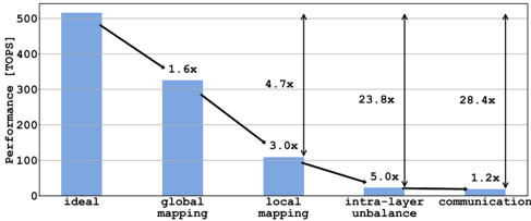
Fig. 6. Performance degradation considering non-idealities due to static mapping, network topology, and communication.
<details>
<summary>Image 6 Details</summary>
### Visual Description
\n
## Bar Chart: Performance Comparison of Mapping Strategies
### Overview
This image presents a bar chart comparing the performance (in TOPS - Tera Operations Per Second) of different mapping strategies. The strategies are "ideal", "global mapping", "local mapping", "intra-layer unbalance", and "communication". Arrows indicate the performance degradation between each step.
### Components/Axes
* **X-axis:** Mapping Strategy (Ideal, Global Mapping, Local Mapping, Intra-layer Unbalance, Communication)
* **Y-axis:** Performance [TOPS]. The scale ranges from 0 to 500, with increments of 100.
* **Bars:** Represent the performance of each mapping strategy. The bars are a light blue color.
* **Arrows:** Indicate the performance reduction from one strategy to the next. The arrows are black and labeled with a multiplier indicating the performance degradation.
### Detailed Analysis
The chart shows a significant decrease in performance as the mapping strategy moves from "ideal" to "communication".
* **Ideal:** Performance is approximately 510 TOPS.
* **Global Mapping:** Performance drops to approximately 320 TOPS. The arrow indicates a 1.6x performance reduction.
* **Local Mapping:** Performance further decreases to approximately 100 TOPS. The arrow indicates a 3.0x performance reduction.
* **Intra-layer Unbalance:** Performance drops to approximately 40 TOPS. The arrow indicates a 4.7x performance reduction.
* **Communication:** Performance reaches a minimum of approximately 20 TOPS. The arrow indicates a 5.0x performance reduction. An additional arrow from the "Intra-layer Unbalance" bar to the "Communication" bar indicates a 23.8x performance reduction, and another from the Y-axis to the "Communication" bar indicates a 28.4x performance reduction.
### Key Observations
* The largest performance drop occurs between "local mapping" and "intra-layer unbalance".
* The "ideal" performance is significantly higher than all other strategies.
* The "communication" strategy exhibits the lowest performance.
* The performance degradation is not linear; the rate of decrease varies between strategies.
### Interpretation
The data suggests that the mapping strategy has a substantial impact on performance. Moving away from an "ideal" mapping configuration leads to significant performance losses. The "communication" strategy is particularly detrimental, indicating that communication overhead or limitations are a major bottleneck. The large multipliers associated with the arrows highlight the severity of the performance degradation at each step. The chart implies that optimizing the mapping strategy is crucial for achieving high performance, and that addressing communication issues is particularly important. The "intra-layer unbalance" strategy appears to be a critical point of failure, as it leads to a dramatic performance drop. The chart does not provide information on *why* these performance differences occur, only that they *do* occur. Further investigation would be needed to understand the underlying causes of the performance degradation.
</details>
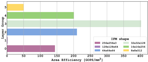
Fig. 7. Area efficiency per group of clusters as defined in Fig. 2 without communication inefficiencies.
<details>
<summary>Image 7 Details</summary>
### Visual Description
\n
## Bar Chart: Area Efficiency vs. Layer Group
### Overview
This is a horizontal bar chart illustrating the relationship between Area Efficiency (measured in GOPS/mm²) and Layer Group, categorized by IFM (Input Feature Map) shape. The chart displays the area efficiency for six different layer groups, each represented by a distinct color corresponding to a specific IFM shape.
### Components/Axes
* **X-axis:** Area Efficiency [GOPS/mm²], ranging from 0 to 400, with tick marks at 50, 100, 150, 200, 250, 300, 350, and 400.
* **Y-axis:** Layer Group, ranging from 0 to 5, with tick marks at each integer value.
* **Legend:** Located in the top-right corner, detailing the IFM shape associated with each color:
* Magenta: 256x256x3
* Purple: 128x128x64
* Blue: 64x64x64
* Light Green: 32x32x128
* Green: 16x16x256
* Yellow: 8x8x512
### Detailed Analysis
The chart consists of six horizontal bars, each representing a layer group. The length of each bar corresponds to its area efficiency.
* **Layer Group 0 (Magenta):** The bar extends to approximately 120 GOPS/mm².
* **Layer Group 1 (Purple):** The bar extends to approximately 190 GOPS/mm².
* **Layer Group 2 (Blue):** The bar extends to approximately 210 GOPS/mm².
* **Layer Group 3 (Light Green):** The bar extends to approximately 320 GOPS/mm².
* **Layer Group 4 (Green):** The bar extends to approximately 380 GOPS/mm².
* **Layer Group 5 (Yellow):** The bar extends to approximately 60 GOPS/mm².
The bars are arranged vertically, with Layer Group 0 at the bottom and Layer Group 5 at the top.
### Key Observations
* Layer Group 4 exhibits the highest area efficiency, at approximately 380 GOPS/mm².
* Layer Group 5 exhibits the lowest area efficiency, at approximately 60 GOPS/mm².
* Area efficiency generally increases with Layer Group, peaking at Layer Group 4, then decreasing at Layer Group 5.
* The IFM shape 16x16x256 (Green) corresponds to the highest area efficiency.
* The IFM shape 8x8x512 (Yellow) corresponds to the lowest area efficiency.
### Interpretation
The data suggests a correlation between Layer Group, IFM shape, and Area Efficiency. The increasing trend in area efficiency from Layer Group 0 to 4 indicates that certain layer configurations are more efficient in terms of GOPS per square millimeter. The significant drop in area efficiency at Layer Group 5 suggests that the chosen IFM shape (8x8x512) for that layer is less optimal.
The relationship between IFM shape and area efficiency is also apparent. The larger IFM shapes (256x256x3, 128x128x64) generally result in lower area efficiencies compared to smaller IFM shapes (16x16x256, 32x32x128). This could be due to increased computational overhead or memory access costs associated with larger feature maps.
The chart provides valuable insights for optimizing neural network architectures by identifying layer configurations and IFM shapes that maximize area efficiency. The outlier at Layer Group 5 warrants further investigation to understand the reasons for its poor performance.
</details>
then scaled to a 5nm tech node more suitable for modern HPC architectures. Fig. 5D shows the execution time of a batch of 16 256 × 256 images on the architecture. For each cluster, it shows the amount of time spent on computation, communication, synchronization, and sleeping. Since analog and digital computations are performed in parallel, execution bars are indicated in green when analog bound and in red when digital bound. We can note an expected increasing trend of latency with the cluster ID caused by the head and tail of the pipeline execution (i.e., idle times waiting for the first and the last batches are propagated through the pipeline).
Fig. 5A shows the performance gain achieved thanks to the techniques described in Sec. IV. Fig. 5B shows the latency breakdown of the clusters in a naive implementation, where all the network parameters are mapped into the architecture exploiting the multi-cluster technique described (Sec. V-1) but with no further optimizations. It is possible to note the large unbalance between the first layers and the deeper layers in the network. Fig. 5C shows the latency breakdown after datareplication and parallelization , better balancing the pipeline and improving performance by 1.6 × at the cost of utilising 61 more clusters. Reducing compute latency moves the bottleneck of the execution on communication due to large contentions on the HBM, mainly caused by residual management. Fig. 5d shows the optimized mapping of residual described in Sec. V-4 further improving performance by 1.9 × at the cost of 2 more clusters (to exploit 2 MB of available on-chip memory).
To provide insights into the sources of inefficiency highlighted in Fig. 5D, we analyze the mapping and latency breakdown of the Resnet-18 inference. The first source of inefficiency (global mapping) is caused by the fact that not all the clusters are used for mapping network parameters. In our mapping, 322 clusters out of 512 have been exploited. This is an intrinsic characteristic of all systolic architectures exploiting pipelining as a computational model, worsened by the constraints in terms of mapping imposed by IMA. However, this has only an effect on the area efficiency since, in such regular architecture, each cluster can be easily clock and power gated, minimizing the impact on energy efficiency. The second source of inefficiency (local mapping) is caused by the fact that even if a specific cluster is being used, the mapping on it might under-utilize the analog and digital resources. In some cases, parameters cannot fill the whole IMA; in other cases, the array is not used at all. The same happens for digital computing, e.g., in the case of purely digital layers. A possible solution to mitigate this degradation could be to integrate heterogeneous clusters configured to fit better all the possibilities, such as IMA and a single CORE (i.e., analog clusters) or 16 CORES without IMA (i.e., digital clusters).
The third source of inefficiency is caused by the pipeline unbalance. Different layers feature different computational efficiency, as described in Fig. 7, where the layer groups are defined depending on the IFM dimension. Some layer groups feature significant area efficiency, thanks to large IFM/OFM implying high data reuse (i.e., several iterations over the same parameters statically mapped on the IMA). In particular, Layer 12 (i.e., group 3) is executed on 10 clusters, with datareplication factor of 2, leading to a peak of efficiency of 600 GOPS/mm 2 . Conversely, deeper layers in the network, because of the stride, feature analog layers with very poor parameters reuse interleaved with stages of reductions executed by the CORES. In particular, Layer 20, 21, 23, and 24 (i.e., group 5) are executed on 40 clusters each. This causes extremely low latency for the execution of the analog layers (less than 0.2 ms), which translates into lower area efficiency (50 GOPS/mm 2 ) compared to the first layers. A possible approach to tackle this inefficiency might lead to further exploiting heterogeneity by coupling IMA and CORES with a set of more compact specialized digital accelerators more suitable for low-data reuse layers, improving the silicon efficiency. Another approach could be to use larger IMA arrays [17]. However, this would require more data transfers per cluster.
Despite the analyzed sources of inefficiency, the proposed architecture delivers 20.2 TOPS (i.e., 3303 images/s) and 42 GOPS/mm 2 on the end-to-end inference of Resnet-18. Performing the inference in 9.2 ms and 15 mJ, which corresponds to an energy efficiency of 6.5 TOPS/W, paves the way for a new generation of general-purpose many-core architectures exploiting a mix of analog and digital computing.
## VII. CONCLUSION
In this work, we have proposed a general-purpose heterogeneous multi-core architecture based on a PULP cluster augmented with nvAIMC accelerators to efficiently execute real end-to-end networks, exploiting the throughput of such a paradigm. We have proposed a mapping based on the combination of pipelining execution flow and many techniques to increase the parallelism and split the workload among the nvAIMC cores. We have shown the results of the inference of a batch of 16 256 × 256 images on a ResNet-18, obtaining up to 20.2 TOPS and 6.5 TOPS/W for a 480 mm2 architecture. We have finally provided an exhaustive performance analysis, considering a real case of traffic and highlighting the criticisms when nvAIMC is used in real applications, providing several insights on how to mitigate this effect, to drive the design and the usage of nvAIMC architecture as a general-purpose platform for DNN acceleration.
## ACKNOWLEDGEMENT
This work was supported by the WiPLASH project (g.a. 863337), founded by the European Union's Horizon 2020 research and innovation program.
## REFERENCES
- [1] A. Sebastian et al. , 'Memory devices and applications for in-memory computing,' Nature nanotechnology , vol. 15, no. 7, pp. 529-544, 2020.
- [2] J.-s. Seo et al. , 'Digital Versus Analog Artificial Intelligence Accelerators: Advances, trends, and emerging designs,' IEEE Solid-State Circuits Magazine , vol. 14, no. 3, pp. 65-79, 2022.
- [3] J.-M. Hung et al. , 'Challenges and Trends of Nonvolatile In-MemoryComputation Circuits for AI Edge Devices,' IEEE Open Journal of the Solid-State Circuits Society , vol. 1, pp. 171-183, 2021.
- [4] S. Yu et al. , 'Compute-in-Memory Chips for Deep Learning: Recent Trends and Prospects,' IEEE Circuits and Systems Magazine , vol. 21, no. 3, pp. 31-56, 2021.
- [5] H. Jia et al. , '15.1 A Programmable Neural-Network Inference Accelerator Based on Scalable In-Memory Computing,' in 2021 IEEE International Solid- State Circuits Conference (ISSCC) , vol. 64, pp. 236238, 2021.
- [6] I. A. Papistas et al. , 'A 22 nm, 1540 TOP/s/W, 12.1 TOP/s/mm2 inMemory Analog Matrix-Vector-Multiplier for DNN Acceleration,' 2021 IEEE Custom Integrated Circuits Conference (CICC) , pp. 1-2, 2021.
- [7] R. Khaddam-Aljameh et al. , 'HERMES-Core-A 1.59-TOPS/mm2 PCM on 14-nm CMOS In-Memory Compute Core Using 300-ps/LSB Linearized CCO-Based ADCs,' IEEE Journal of Solid-State Circuits , vol. 57, no. 4, pp. 1027-1038, 2022.
- [8] H. Jia et al. , 'A Programmable Heterogeneous Microprocessor Based on Bit-Scalable In-Memory Computing,' IEEE Journal of Solid-State Circuits , vol. 55, no. 9, pp. 2609-2621, 2020.
- [9] A. Garofalo et al. , 'A Heterogeneous In-Memory Computing Cluster for Flexible End-to-End Inference of Real-World Deep Neural Networks,' IEEE Journal on Emerging and Selected Topics in Circuits and Systems , vol. 12, no. 2, pp. 422-435, 2022.
- [10] C. Zhou et al. , 'AnalogNets: ML-HW co-design of noise-robust TinyML models and always-on analog compute-in-memory accelerator,' arXiv preprint arXiv:2111.06503 , 2021.
- [11] M. Dazzi et al. , 'Efficient Pipelined Execution of CNNs Based on In-Memory Computing and Graph Homomorphism Verification,' IEEE Transactions on Computers , vol. 70, no. 6, pp. 922-935, 2021.
- [12] A. Shafiee et al. , 'ISAAC: A Convolutional Neural Network Accelerator with In-Situ Analog Arithmetic in Crossbars,' in 2016 ACM/IEEE 43rd Annual International Symposium on Computer Architecture (ISCA) , pp. 14-26, 2016.
- [13] A. Ankit et al. , 'PUMA: A Programmable Ultra-Efficient MemristorBased Accelerator for Machine Learning Inference,' in Proceedings of the Twenty-Fourth International Conference on Architectural Support for Programming Languages and Operating Systems , ASPLOS '19, (New York, NY, USA), p. 715-731, Association for Computing Machinery, 2019.
- [14] N. Bruschi et al. , 'GVSoC: A Highly Configurable, Fast and Accurate Full-Platform Simulator for RISC-V based IoT Processors,' in 2021 IEEE 39th International Conference on Computer Design (ICCD) , pp. 409-416, 2021.
- [15] M. Gautschi et al. , 'Near-Threshold RISC-V Core With DSP Extensions for Scalable IoT Endpoint Devices,' IEEE Transactions on Very Large Scale Integration (VLSI) Systems , vol. 25, no. 10, pp. 2700-2713, 2017.
- [16] A. Kurth et al. , 'An Open-Source Platform for High-Performance NonCoherent On-Chip Communication,' IEEE Transactions on Computers , pp. 1-1, 2021.
- [17] P. Narayanan et al. , 'Fully On-Chip MAC at 14 nm Enabled by Accurate Row-Wise Programming of PCM-Based Weights and Parallel VectorTransport in Duration-Format,' IEEE Transactions on Electron Devices , vol. 68, no. 12, pp. 6629-6636, 2021.